new class of growth models for even-aged stands: pinus radiata in golden downs … ·...

65

NEW CLASS OF GROWTH MODELS FOR EVEN-AGED STANDS: PINUS RADIATA

IN GOLDEN DOWNS FOREST. OSCAR GARCIA

Forest Research Institute, New Zealand Forest Service, Private Bag, Rotorua, New Zealand.

(Received for publication 19 December 1983; revision 24 February 1984) ABSTRACT

A methodology for modelling the growth of managed even-aged stands has been developed. The state of a stand is represented by a number of variables — typically basal area, stocking, and top height. Changes of state through growth and mortality are given by a system of differential equations which are a multivariate generalisation of the Bertalanffy-Richards model. For estimation purposes random perturbations are included, and the parameters are estimated by maximum likelihood based on the resulting stochastic differential equations. The growth equations are complemented by models for thinning, early growth, volume per hectare, and diameter distributions. The methods have been applied to the development of a model for Pinus radiata D. Don in Golden Downs Forest, Nelson, with satisfactory results.

INTRODUCTION A methodology for obtaining growth models for even-aged stands has been

developed. The objective is the development of models at the forest and regional level to cover the whole of New Zealand, and the subsequent testing for possibilities of aggregation. The effort will concentrate mainly on the modelling of Pinus radiata plantations.

The models consist of a set of differential equations describing changes in stand variables such as basal area, stocking, and top height. The model parameters are estimated by the method of maximum likelihood, under specific assumptions about the random variation in the model. The likelihood values may be used for evaluating similarities between different data sets and for other hypothesis-testing purposes.

The methods have been applied to the development of models for P. radiata in Golden Downs Forest and in Hawke's Bay, with satisfactory results. Work is in progress on models for P. radiata in Auckland sand dune forests and in Kaingaroa State Forest, and for Pseudotsuga menziesii (Mirb.) Franco in Southland. An earlier model for P. radiata in Southland Conservancy (Garcia 1979) is considered provisional because of deficiencies in the data available.

This paper concentrates on the methodological aspects, and especially on the results of applying the methodology to the Golden Downs data. A more user-oriented description of the Golden Downs model is in preparation. The general philosophical background for the methodology, and the mathematics of the model, have been discussed in more detail previously (Garcia 1979).

An extended version of this paper is available from the author.

New Zealand Journal of Forestry Science 14(1): 65-88 (1984)

66 New Zealand Journal of Forestry Science 14(1)

MODELS AND ESTIMATION PROCEDURES The model uses a state space approach — that is, a sufficient number of variables

describe the "state" of the stand at any given time so that (a) future states are determined by the current state and future actions, and (b) quantities of interest, such as volumes, can be derived from the values of the state variables (Garcia 1979). In other words, the state variables summarise the historical events affecting the future development of the stand. For Golden Downs, it was found that three state variables — basal area, stocking, and top height — gave satisfactory results. A fourth variable, representing a measure of site occupancy after thinning, was tried but its inclusion was found unnecessary. The growth model predicts the changes in the state of the stand caused by tree growth, natural mortality, and thinnings.

The changes in the state variables through tree growth and mortality are described by a set of differential equations. These will be called the growth equations, and may be used to predict the state of the stand in periods between thinnings. For Golden Downs the growth equations are not applicable to very young stands (top height less than about 6 m), and a separate model is used for "starting" a simulation from age zero.

Thinnings cause an instantaneous change of state. The thinning model relates the basal area removed to the number of trees removed, given before thinning values. The model assumes thinnings where the top height does not change.

Given the state variables, volumes for various products may be estimated from stand volume equations or from "stand volume generators" (Goulding & Shirley 1979). A stand volume equation for total standing volume per hectare was derived from the sample plot data. Diameter distributions for use in stand volume generators were also obtained.

Growth Equations The growth equations are a multivariate generalisation of the Bertalanffy-Richards

model taking the following general form (Garcia 1979; the univariate Bertalanffy-Richards model can be written as dxc/dt = axc + b):

dy t = Ay + b (i)

where

y\ yi

CL\\

=

CI 12 01.fi

0>l\ Q>12 #23

0 0 a^\

2,N22H2i

and

6,

b2

b,

B = basal area (rnVha), N = stocking (stems/ha), H = top height (m), t = age (years).

Garcia — Growth models for even-aged stands 67

The third equation in (1) represents the height growth (site index curves) and was estimated separately beforehand (Garcia & Lawrence in prep.). Therefore, the coefficients <Z33> b^ and C33 are here assumed known.

Note that the form of the model does not change if instead of B and N we use other variables which are power transformations of these, such as mean d.b.h. (diameter at breast height) or average spacing.

Previous experience with the model suggested that the number of free parameters in (1) might be excessive, leading to ill-conditioning in the estimation procedure (i.e., different combinations of parameter values result in about the same degree of fit). It also seems desirable to constrain the stocking to be always non-increasing, even outside the range of the data. A simple way of ensuring this, reducing the number of parameters at the same time, is to make a22 = an = b2 = c2\ = en = 0. Then the stocking will always decrease with time, provided that a2\ and c22 have opposite signs.

The coefficients in (1) vary with the site quality. A convenient assumption is that the Cij are independent of site, and A and b change by a constant factor dependent on the site index. This implies that the effect of the site index is a change in the time scale with no effect on the relationships between the state variables. This assumption is compatible with the Golden Downs site index equations (Garcia & Lawrence in prep.), and was found satisfactory in the validation of the model. Given the site index equation of the form

dH° — = b(ac-Hc), (2) at

where b = - In [ 1 - (S/af] / (20 - t0) (3)

and S is the site index, the effect of the site in the model can be conveniently represented by using a "scaled time" r = bt in the place of t.

The specific form of the model which was used is then:

UD iV H c , , c n c , , c~~ c , , , = au B " N 12 H l3 + an N n + an H " + 6,

dr < » ' C 2 2 c . c . c . ;

(4) fliV

dr

dH3i

dr

=

=

aixB

-H»

" N12

+ b,,

C

H 13

where r = bt, with b related to site index through (3). Here 63 and cn are assumed known, specifically, 63 = ac and C33 = c from (2). Defining x = (B,N>H)3 and xc = exp [C In x], (4) may be written using matrix notation as

dxc . r — = Axc + b UT

(5) or c

lt = A(X" " 3)'


where

A =

C =

011

a2\ 0

Cu

0 0

^12

0 0

C\2

Cu

0

013

0

- l j

C\{\

0

^33

bx

b= | 0

and a = - A ' b .

Given the state at time fi, (5) can be integrated to obtain the state at any other time t2 if there are no thinnings between t\ and t2:

x (t2) = {a + p - V b ^ - '0 P [x(tOc - a]} c_1 (6)

Here P and A are such that A is diagonal and

A = P A P ,

that is, the elements on the diagonal of A are the eigenvalues of A (assumed to be real and distinct, see Garcia 1979), and the rows of P are the left eigenvectors. A slightly more complex equation could be used if A were a singular matrix (Appendix).

Estimation To estimate the parameters we assume that the growth described by (4) is perturbed

by random terms added to the right-hand sides. These random terms are assumed to be stationary Gaussian random processes with independent increments (i.e., Wiener or Brownian motion processes). The three processes may be cross-correlated, and the elements of the covariance matrix are additional parameters to be estimated from the data.

The Equations (4) with the random components added constitute a set of stochastic differential equations, which can be integrated to obtain the probability distribution of the state at any time given the state at some other time (provided that there are no thinnings in between). In particular, for each pair of consecutive measurements with no thinnings between them, and for a given set of parameters, we can compute the probability of observing the second measurement given the first one. Assuming statistical independence between plots, these probabilities may be aggregated over all the data to obtain the probability of generating the observed data from the given model (Garcia 1979). This probability, considered as a function of the parameters, is called a likelihood function, and the method of maximum likelihood (ML) consists of selecting as estimates the values of the parameters which maximise the likelihood.

Estimation is simplified if it is assumed that the covariance matrix for the stochastic process is diagonal after an eigenvector transformation (Appendix). We shall call Method I the ML estimation under this assumption, and Method II the ML estimation using the more general covariance matrix. The respective likelihood functions are shown in the Appendix.


Both Methods I and II were tried. The parameter estimates were obtained by maximising the log-likelihood with a general-purpose optimisation algorithm (Biggs 1971, 1973; N.O.C. 1976).

"Thinning Effect" It seems plausible that after heavy thinnings some growth could be necessary for the

residual trees to make full use of the additional resources made available to them by the removal of competitors. Therefore, it might be expected that the growth immediately after a thinning would be less than that of a stand of similar basal area, stocking, and height, but not recently thinned.

An extension of the basic growth model (4) was tried in an attempt at modelling this "thinning effect". However, the results from fitting this extended model were negative, and examination of the prediction residuals from (4) also failed to show any evidence of reduced growth after thinning. For completeness, the extended model is described here, and the results are discussed further under "Model Fitting and Results". This model was later tried with satisfactory results on a data set for P. radiata in Hawke's Bay.

The data available did not contain enough measurements of green crown level for using this as a variable, so that an artificial measure of "relative site occupancy" was used. The relative site occupancy, J?, at the time of a thinning was taken as the ratio of basal area after thinning to the basal area before thinning. After the thinning R was assumed to increase towards an asymptotic value of 1. Specifically, the following extension of (4) was used:

'dBuNnHnRu _ c i i c n c t - 3 _ c

dr

dN22R24

dr dH"

dr

dR44

dr

= an B"N,2H"RU + au N22R24 + al3 H13 + a» R44 + bx

= a21Bc"Nc,2//C|3/?Cl4

(7)

— (244 -** — (244.

For R = 1 (full site occupancy) this model is equivalent to (4). For estimation purposes, only the first three equations in (7) are assumed to have a

random perturbation on the right-hand side. Since there are no observations ofR other than at the time of thinnings, the fourth equation in (7) is taken as deterministic, and may be solved as:

R = [\-(l-R0 4A)e 44 ] 4 4 , (8)

where RQ is the thinning ratio (ratio of basal area after thinning to basal area before thinning) for the last thinning, T is the time elapsed since the last thinning, and b is given by (3).


Model (7) was also tried with a\4 = C2A - 0. The predicted R was always found to approach 1 too slowly. Therefore, (8) was also constrained so that J? would increase from 0.5 to 0.99 in 4 years for site index 27. This additional constraint is:

1 - 0.99C44

a44 = 3.9036 In t44. (9)

Thinnings The thinning model is used to predict the basal area removed in a thinning given the

number of trees removed, or vice versa. It is desirable for the model to be closed under composition. That is, removal of 40 stems/ha followed by removal of 60 stems/ha should result in the same final basal area as the removal of 100 stems/ha. This type of consistency is ensured with a model based on a differential equation for the change in basal area relative to the change in stocking. The general form of the equation used may be written as

iH =-BbN^H\ (10) d In N

where a, b, c> and d are parameters to be estimated. On integration this gives InB = - In [ Bo ~h - ab

cHd(Nc - N0

C) ] /b, (11) if b and c are different from zero. Here B0 and No are the basal area and stocking before thinning and B and N those after thinning.

Equation (10) is mathematically convenient and fairly flexible; for example, the model used by Elliott & Goulding (1976) corresponds to the special case of b = c = d = 0.

Equation (11) was fitted with a nonlinear least-squares procedure to the thinning data. The equations obtained from (10) with 6, c, or d equal to zero were also tried. It was found that making b = 0 had a negligible effect on the prediction error, so that this simpler equation was used. The integrated form is

In B = In Bo + acH

d (Nc - NQC). (12)

Early Growth The differential equations described well the growth within the range of the data

available but were found to be unreliable for top heights less than about 6 m. A separate model for "starting" simulations beginning at age zero was needed.

A simple model for early growth was used to derive a relationship between basal area and stocking at a given height. Let U be some measure of "site occupancy", such as crown cover or leaf area index, assumed to be related to basal area and stocking by

U=aB + pN>'<x,P>0, (13) until it reaches a maximum of t/max (full site occupancy, crown closure), after which it remains constant. The motivation for the second term on the right-hand side in (13) is that for B = 0 at H = 1.4 m there would be some site occupancy fi per tree. Assume that the basal area growth is proportional to U:


dB — =f(H9r)U, (14)

where/(//, r) is any arbitrary function of the height and the adjusted time, and that there is no mortality. Then, it can be shown that for any given top height,

((a/c-b)N , for N^c B= < (15)

\a]nN-bN + a(l-kic), forN^c, where <z, b, and c are constants. The parameter c depends on the height, while a and b do not.

A more general model may be obtained by using

^ =f(H, r ) U 7 (16) dr

instead of (14).

DATA Golden Downs State Forest is located in the Nelson district, near the northern end of

the South Island of New Zealand (latitude 41.5°S, longitude 173°E). It is the second-largest exotic forest owned by the N.Z. Forest Service, with 22 400 ha of P. radiata and 9170 ha of other species.

The data were obtained from the Forest Service Permanent Sample Plot (PSP) System {see McEwen 1979 for a description of the PSP System and details of the computation of top height and volume).

The data for the growth equations were screened according to a number of criteria. Plots flagged in the PSP System as abnormal or unsuitable for growth modelling and plots in naturally regenerated stands were excluded. Also excluded were measurements taken after application of fertilisers or poison thinning, and measurements with missing or insufficient data (at least eight height sample trees were required). Increment periods with more than two windblown trees in the plot, or where the mean d.b.h. of the windblown trees exceeded the mean d.b.h. for the plot, were not used. If necessary, the ages were adjusted for date of measurement as described by Garcia (1979), and measurements in November to January, where no satisfactory adjustment is possible, were eliminated.

The final data set for the growth equations consisted of 469 measurements from 119 different plots, forming 339 measurement pairs. The selected data are plotted in Fig. 1. Some limitations in coverage can be seen from the graphs. There are no data for very young stands, and data from very old stands are unreliable because of large relative errors in the height increments caused by a combination of slow growth, broken tops, and large measurement errors (several older plots show negative height increments). Also there is little information from dense (unthinned) stands, and their trends are rather erratic. These trends are probably due, at least in part, to the normal variability in natural mortality: mortality is likely to be concentrated in years when climatic conditions are unfavourable. The graphs in Fig. 1 give an indication of those values of the state variables for which the model would be unreliable.

New Zealand Journal of Forestry Science 14(1)

20 25 TOP HEIGHT (m)

15 20 25 30 AGE (years)

40 45

FIG. 1 — Measurements from the 119 sample plots forming the data base


Other limitations of the data should be mentioned. The PSP System contains no information on pruning, and that contained in "plot history sheets" was found to be incomplete and unreliable. Any effects of pruning on growth would be confounded with the effect of thinnings through the values of the state variables. The model would reflect the average pruning usually applied in conjunction with thinnings. Also, information on green crown levels was available for very few plots, thus precluding any attempt at using this variable for accounting for pruning and thinning effects.

MODEL FITTING AND RESULTS Height Growth

The general model used was (2) or, integrated with initial condition H — 0 at t = r0,

H = a[\-e-h^-i°)}l/c (17) To obtain a family of site index curves, one parameter (or some function of the parameters) in these equations must vary from plot to plot as a function of the site index, with the rest of the parameters being the same for all plots.

An error structure containing both measurement errors and environmental variation was assumed, and all the parameters were estimated simultaneously by maximum likelihood. Models with the site-indexing parameter a> b, or a linear function of a and b were tried. Best results were obtained with b as the indexing parameter. It was also found that a non-zero value for t0 resulted in a better fit to the data. The fitting of the height growth model is described in detail by Garcia & Lawrence (in prep.) and the methodology by Garcia (1983). The parameter estimates are

a =51.752

c =0.41272

fo = -2.5793 (height in metres, age in years). The value of b is obtained from (17) with the site index5 :x 5 substituted for the height at age 20 (Equation (3)).

Basal Area and Stocking Site index

For most plots the site index needed for fitting the growth model was obtained in the ie process of developing the site index curves. For plots not used in the height growth model, the site index was estimated as the average of the site indices corresponding to each height-age measurement. Early growth

It is often necessary to predict the development of a hypothetical stand from the time ie of planting. The unconstrained model fitted to the available data, however, cannot be expected to give good predictions starting at age zero. Two solutions to this problem were tried. One is to use the model only for ages close to those represented in the data, and to develop a separate model for predicting the early growth (as described in a previous section). The second one is to somehow constrain the model so that it behaves s reasonably well at very young ages not represented in the data.


This second approach was implemented as follows. The initial growth in a stand is free from competition between the trees, so that it may be assumed that the mean d.b.h. for young stands is a function only of height, independent of the stocking. Examination of some data from young stands and backward projections with the unconstrained model suggested as reasonable a mean d.b.h. of 5 cm at top height 4 m. All initial measurements of plots which had not been thinned before the first measurement, were collected. Using information on the initial spacing, if available, and/or Beekhuis' (1966) mortality curves, an estimate of the stocking at top height 4 m for each of these plots was obtained, and the basal area calculated assuming a mean d.b.h. of 5 cm. The result of this was an extra set of 40 artificial "measurement" pairs covering early stand growth. We shall refer to the data set consisting of the actual 339 measurement pairs plus the 40 artificial pairs s the "extended data set". Given only the initial spacing, a model fitted to the extended data set could be used to predict the development of a stand by starting the model at top height 4 m with a mean d.b.h. of 5 cm. Results

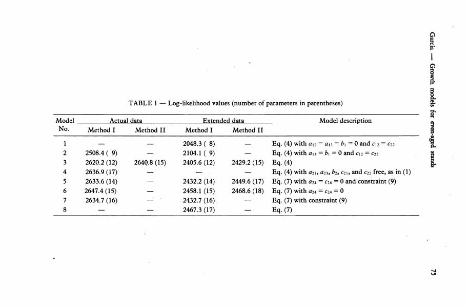
A number of variations on the Models (4) and (7), using estimation Methods I and II and the actual and extended data sets, were tried. The main results are summarised in Table 1, which shows the maximised log-likelihoods. For a given set of data, different models may be compared by considering the number of parameters and the difference in the maximised log-likelihoods. There is no fully satisfactory theory for comparing models, but several different arguments suggest subtracting from the maximised log-likelihood one-half to three units for each additional parameter, and viewing differences of more than two units after this adjustment as "significant" (see Garcia 1979, 1983; Atkinson 1980). The values for the actual and for the extended data sets are not directly comparable, and some other ways of comparing these are discussed below.

An extensive analysis was also carried out with an earlier version of the data set which was found later to contain a few measurement errors. The results generally agree with those shown in Table 1.

The likelihood maximisation was performed using the subroutine OPVM written by Hatfield Polytechnic's Numerical Optimisation Centre (N.O.C. 1976; Biggs 1971, 1973), with numerical approximation for the derivatives. In general, the estimation procedure performed well although, especially for the models with large numbers of parameters, good initial estimates were usually needed for converging to a solution in a reasonable number of iterations. For this reason, whenever possible the parameter estimates for a model were used as the starting point for estimating the parameters of the next more-general model. Also, estimates for the actual data set were frequently used as starting values for models fitted to the extended data set, and Method I estimates were used as starting values for Method II. Often the estimates were checked by starting the optimisation procedure from different points; no instances of multiple local optima were found. Model selection

Models 5 to 8 (Table 1), which include adjustments for "thinning effect", seemed to fit the data better than the others. However, when basal area increments were computed with these models it was found that values of the "site occupancy" R smaller than one generally gave higher increments than for stands fully occupying the site (R = lj. Therefore, these models are unacceptable.

f I

TABLE 1 — Log-likelihood values (number of parameters in parentheses) §-

ft 3 ? 2L

Model No.

1 2 3 4 5 6 7 8

Actual data Method I

— 2508.4 ( 9) 2620.2(12) 2636.9(17) 2633.6 (14) 2647.4(15) 2634.7 (16)

—

Method II

—

— 2640.8 (15)

— — — — —

Extended data Method I

2048.3 ( 8) 2104.1 ( 9) 2405.6 (12)

— 2432.2 (14) 2458.1 (15) 2432.7 (16) 2467.3 (17)

Method II

—

— 2429.2 (15)

— 2449.6 (17) 2468.6 (18)

— —

Model description

Eq. (4) with a\2 = an = Ji = 0 and c\2 = c22

Eq. (4) with an=b\=0 and cn — c22

Eq. (4) Eq. (4) with a2l, a23, b2, c2\, and c22 free, as in (1) Eq. (7) with a24 = c24 = 0 and constraint (9) Eq. (7) with a24 = c24 = 0 Eq. (7) with constraint (9) Eq. (7)


Models 1 and 2, and other simpler models tried with the initial data set, are specialisations of the equations in (4). They were obtained by constraining the model to satisfy some common forestry hypothesis, such as independence between gross basal area increment and stocking, existence of an invariant relationship between /?, N, and// (Decourt 1974), and the asymptotic relationships implied by Reineke's (1933) density index and Beekhuis' (1966) mortality model. These models are clearly inferior to Model 3, and therefore will not be discussed further. They were useful, however, in providing initial estimates for the parameters in the other models.

For completeness, a model including the free parameters #22? # 2 3 j 62,C2i,andc235asin Equation (1), was fitted (Model 4 in Table 1). This appears to fit the data somewhat better than Model 3. However, 4 sometimes predicts stockings increasing with time, although this happens outside the range of the data. It seems then preferable to use Model 3 which is constrained to produce reasonable predictions over the whole state space.

Graphical examination of the predictions from Model 3 fitted to the actual and to the extended data sets showed very small differences for the region of the state space where most of the data are found, but larger differences at the extremes, e.g., for high basal areas and top heights. As expected, the predictions from the model fitted to the actual data appeared in general closest to the observed values. A measure of the differences was obtained by computing the log-likelihood for the parameter estimates obtained with the extended data set when applied to the actual data. This log-likelihood differed from the optimum by 30.7 units for Method I and by 236.1 units for Method II. This indicates that trying to force the model to be applicable to very young stands resulted in a substantial loss of accuracy in the predictions for stands represented in the data. It was decided then to use the model fitted to the actual data and to use a different procedure for estimating the growth of young stands.

Comparison of the log-likelihoods between Method I and Method II would indicate a better fit for Method II (the two methods are based on different models for the random components). The results of Method II for Model 3 on the actual data set were somewhat peculiar in that the optimal value of a\ i was close to zero, which implies that

Ai is approximately equal to - A: and corresponds to a discontinuity in the computed likelihood (Appendix). This did not happen with the extended data set. Graphical comparisons of the basal area and mortality predictions from Model 3 fitted with Methods I and II showed relatively small differences. The adequacy of the models was examined further by plotting the computed eigenvectors as suggested by Garcia (1979). The graphs for Model 3 fitted with Method II showed large deviations from the expected pattern (details are available from the author). Method I would also appear to have advantages in relation to some proposed techniques for studying the effect of fertilisers, heavy thinning, pruning, and other factors, making use of the computed eigenvalues and eigenvectors. For all these reasons, the model obtained with Method I was selected. It may be mentioned, however, that Method II has given satisfactory results in a model for Auckland sand dune forests, currently under development.

The model finally selected is then Model 3 (i.e., Equations (4)), fitted with Method I to the actual (not extended) data set. The parameter values are shown in Table 2.

Garcia — Growth models for even-aged stands

TABLE 2 — Parameter estimates

77

Parameters:

C =

A -

b =

r0.482 83 0 0

"0.452 84 8.379 OX IO"4

_0

"7.205 3~ 0

_ 5.097 7_ Computed eigenvalues, etc.:

Xi = X2 =

x 3 =

P =

-0.451 2< -0.00155 -1

Units: g(m2/ha) , AT (ster

)0 3 48

n 0.001 856 68

Lp ns/ha), H (m)

-0.159 56 -0.524 58 0

-0.836 70 0 0

a =

1.85401 1 0

0.231 54 0 0.412 72_

-0.488 33" 0

-1

"0 5.636 33 5.097 73_

-0.889 958 -0.000 908 079 1

Evaluation For each measurement pair, the values of the state variables at the time of the second

measurement were predicted given the values of the first measurement. Figure 2 compares the basal area and spacing predictions with the observed values. In Fig. 3 the prediction residuals are shown in a form that would facilitate the detection of any systematic biases. Here the value of the ordinate for the first point of each line segment is the first measurement. The value of the ordinate for the point corresponding to the second measurement is the prediction residual added to the value of the first measurement. The predicted height was used for the abscissa. Thus, the slope of the line represents the prediction error relative to the height increment between measurements, and the graphs show how these errors vary for different values of the state variables. Ideally, all the lines should be horizontal.

Basal area predictions appear satisfactory over the range of values for which there are adequate data. Predictions are more uncertain for dense unthinned stands, where there are few data and the trends are erratic owing to the effects of mortality. The model can only predict an "average" mortality, and any particular stand may be expected to deviate substantially from this value. The graphs also show large deviations for old stands; these deviations result mainly from the large relative measurement errors for the height increments.

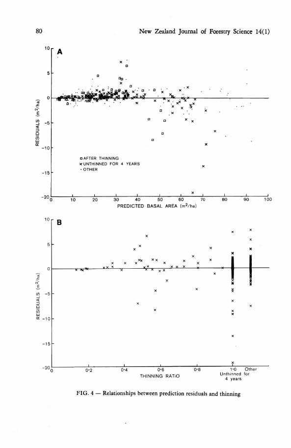
Any substantial thinning effect would be apparent in Fig. 4. Figure 4a shows the differences between observed and predicted basal areas for the second measurement of each measurement pair, for measurement pairs immediately after a thinning, at least 4


"lOOr


40 45

10r

CD

z O CO

LU

CD < a: LU > <

2r

10 15 20 25 30 TOP HEIGHT (m)

35 40 45

FIG. 2 — Comparison of measurements and model predictions

years after thinning, or at intermediate times. Figure 4b shows the same residuals plotted v. the thinning intensity, expressed as the ratio of basal area after thinning to the basal area before thinning. Extensive plotting of computed eigenvalues and eigenvectors also failed to show any evidence of thinning effect.

A similar graphical analysis was done for checking the hypothesis that site index was adequately accounted for by the time-scaling factor (Fig. 5).


100

80 F

E 60 h

< LU a: < < CO < DO

40 h

20 U

15 20 25 TOP HEIGHT (rp)

45


FIG. 3 — Prediction residuals (see text)

The expected prediction errors are a complicated function of the state variables and of the length of the time interval over which the prediction is made. It is traditional with regression models to give standard errors and confidence intervals for the parameters and sometimes for the predictions, always computed under the assumption that the model is "true". This could be done for the present model, but we think that it would be unrealistic and difficult to interpret. Direct graphical comparisons with the dat& as shown above, appear to be much more useful for assessing the reliability of predictions


10 r

°D .

-«j»^xjf x »xV .^x y

x x . *

< g CO LD

tr

- 5

-io r

-15 h

a AFTER THINNING XUNTHINNED FOR 4 YEARS • OTHER

- 2 0 _i I I L- _l L. I l 0 10 20 30 40 50 60 70

PREDICTED BASAL AREA (m 2 /ha)

80 90 100

1 0 r B

5h

X X X x x x x

co - 5 ^ _ i

< Q

* - 1 0

-15 h

-20 j; 0-2 0-4 0-6

THINNING RATIO

0-8 1-0 Other Unthinned for

4 years

FIG. 4 — Relationships between prediction residuals and thinning

Garcia — Growth models for even-aged stands

10 r

81

_ o fe! ft-t ;:j

-5

- 1 0

-15

-20 —I 36 16 18 20 22 . 24 26 28

SITE INDEX (m) 30 32 34

FIG. 5 — Relationship between prediction residuals and site index

TABLE 3 — Measurement pair residuals Mean time interval: 2.02 years

Mean RMS

Basal area (m2/ha) Stocking (stems/ha) Top height (m) Mean d.b.h. (cm) Average spacing (m) Basal area X height (mVha)

-0.051 0 -2.92 0.071 1 0.049 8

-0.004 72 -3.06

2.26 64.1 0.696 0.655 0.086 2 79.8

for various regions of the state space. It is also intended to study methods of prediction error estimation by regression of transformed residuals on functions of the state variables and prediction time interval. Some summary statistics for the residuals* are given in Table 3. Notice that the residuals include the effect of measurement errors.


Early Growth Since there were no data available for very young stands, it was decided to use the first

measurement of the plots which had not been previously thinned, and project these measurements, backwards or forwards, to a common top height using the growth equations. These points were then used for estimating the parameters in (15). Only measurements in which the top heights were less than 15 m (38 measurements) were used.

Equation (15) predicts that B should be directly proportional to N for N between 0 and c. Projecting the first measurements of the unthinned plots to various heights using the growth equations showed this relationship to be approximately linear for H = 7 m, but not for other values of//. This may be an artifact caused by the form of the growth equations, or it may be that the assumptions behind (15) are too unrealistic. A more general model based on (16) could have been used, but it was felt that the information available did not justify the additional complexity at this stage. It was decided then to fit (15) for H = 7 m. Thinnings at less than 7 m top height are therefore not catered for (none were present in the data).

Estimating the parameters in (15) by nonlinear least-squares using the measurements projected to top height 7 m resulted in

fo.0079430 JVifAT< 1711.2 B= (18)

(44.614 In N - 0.018128 JV - 287.54, otherwise. It must be pointed out that these estimates only represent an "average" based on the

available sample plot data. Actual basal areas at height 7 m will be affected by such things as establishment techniques, frosts, and weed competition.

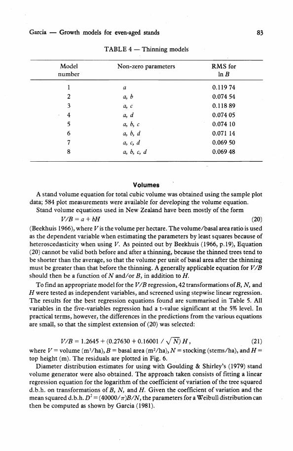
Thinnings All models based on (10) with some combinations of the parameters b, c, and d equal

to zero were tried. The parameters were estimated by integrating (10) to obtain equations for In B as a function of N, H, BQ, and N09 and using a nonlinear least-squares procedure on these equations. Data from 59 thinnings were used, consisting of top height and basal area and stocking before and after thinning.

The root-mean-squared errors for In B for the different models are shown in Table 4. Model 7 was selected, since it fits the data almost as well as the full Model 8, and appears better than the best two-parameter Model 4. The fitted model is:

B = Bo exp [ - 31.891 H -°-28330 (N -°-094574 - No -°-°94574)] , (19)

where H is the top height (m), BQ and B are the basal areas before and after thinning (mVha), and NG and N are the stocking before and after thinning (stems/ha). Notice that the model may also be used to estimate the basal area before thinning given the basal area after thinning.

This model represents an average based on the thinnings performed on the sample plots. Actual values may vary depending on the selection criteria used.

Model number

1 2

3 4

5 6

7

8

Non-zero p

a

a, b

a, c

a, d

a, b, c

a, by d

a, c, d

a, b, c, d


TABLE 4 — Thinning models

neters RMS for

\nB

0.119 74 0.074 54 0.118 89 0.074 05 0.074 10 0.071 14 0.069 50 0.069 48

Volumes A stand volume equation for total cubic volume was obtained using the sample plot

data; 584 plot measurements were available for developing the volume equation. Stand volume equations used in New Zealand have been mostly of the form

V/B = a + bH (20) (Beekhuis 1966)., where Fis the volume per hectare. The volume/basal area ratio is used as the dependent variable when estimating the parameters by least squares because of heteroscedasticity when using V. As pointed out by Beekhuis (1966, p. 19), Equation (20) cannot be valid both before and after a thinning, because the thinned trees tend to be shorter than the average, so that the volume per unit of basal area after the thinning must be greater than that before the thinning. A generally applicable equation for V/B should then be a function of N and/or B, in addition to H.

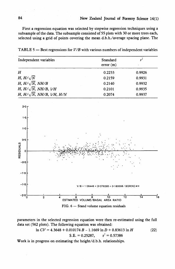
To find an appropriate model for the V/B regression, 42 transformations of B, N, and H were tested as independent variables, and screened using stepwise linear regression. The results for the best regression equations found are summarised in Table 5. All variables in the five-variables regression had a t-value significant at the 5% level. In practical terms, however, the differences in the predictions from the various equations are small, so that the simplest extension of (20) was selected:

V/B = 1.2645 + (0.27630 4- 0.16001 / y/W) H, (21)

where V = volume (mVha), B = basal area (rnVha), N = stocking (stems/ha), and H = top height (m). The residuals are plotted in Fig. 6.

Diameter distribution estimates for using with Goulding & Shirley's (1979) stand volume generator were also obtained. The approach taken consists of fitting a linear regression equation for the logarithm of the coefficient of variation of the tree squared d.b.h. on transformations of B, N, and H. Given the coefficient of variation and the mean squared d.b.h. D2 = (40000/7r)B/Ny the parameters for a Weibull distribution can then be computed as shown by Garcia (1981).


First a regression equation was selected by stepwise regression techniques using a subsample of the data. The subsample consisted of 55 plots with 30 or more trees each, selected using a grid of points covering the mean d.b.h./average spacing plane. The

TABLE 5 — Best regressions for V/B with various numbers of independent variables

Independent variables Standard error (m)

H

H, H/>jN H, H/y/N9 NH/B H, H/sfN, NH/B, VH H, H/y/N, NH/B, VH, H/N

0.2233

0.2159

0.2140

0.2101

0.2074

0.9926

0.9931

0.9932

0.9935

0.9937

2-0

1-5

1-0

0-5 CO - j < 9 o CO LD

tr

-0-5

-1-0

-1-5h

*ft :;^<&?^x':^^o," ;•';-

-2-0

V / B = 1-26446 + [0-276295 + 0-160008/SQR(N)] * H

6 8 10 12 ESTIMATED VOLUME/BASAL AREA RATIO

FIG. 6 — Stand volume equation residuals

14 16

parameters in the selected regression equation were then re-estimated using the full data set (562 plots). The following equation was obtained:

In CV = 4.3648 + 0.010174 B - 1.1669 In D + 0.83613 In H (22) S.E. = 0.25287, r2 = 0.57386

Work is in progress on estimating the height/d.b.h. relationships.


Caution should be exercised in using d.b.h. distributions. It is not generally recognised that distributions based on sample plots may differ from the distributions for whole stands or compartments, which are the ones usually required in the applications. There is a spatial autocorrelation for tree size, negative at short distances owing to competition, and positive over longer distances owing to microsite similarities (see Bouchon 1979 and references therein). This implies that the variance of a d.b.h. distribution would vary with the size of the area considered, although the practical significance of this variation is an open question.

DISCUSSION AND CONCLUSIONS

The general methodology developed here gave satisfactory results and can be used to develop models for other regions and/or species.

The cause for the apparent absence of a "thinning effect" in Golden Downs Forest is not clear. The model described in the section "Thinning Effect" has been found to be satisfactory for P. radiata in Hawke's Bay, and a model with a four-dimensional state space has been developed for this region.

The main limitation of these two models is probably the exclusion of pruning effects, because of the lack of pruning information in the basic data. It is likely that pruning could be handled satisfactorily through a fourth stand variable, as outlined under "Thinning Effect". It is intended to investigate this further when developing a model for Kaingaroa Forest, where a number of pruning experiments exist.

The handling of site index through a time-scale factor as done here would be adequate only when the height-age curves have common asymptotes. For some forests, models where the height asymptotes change with site index may be more adequate. The best way of introducing site index in the growth model for these would probably be through a scale factor for the asymptote vector a. This has been found satisfactory for P. radiata in Auckland sand dune forests.

After a number of models become available, it would be interesting to find out if some of the regions or forests could be represented by common models. This could be tested by fitting models with the pooled data and comparing the log-likelihood for the common model with the sum of the log-likelihoods for the separate models.

Although these methods and models appear to be an improvement over known alternatives, it is clear that some aspects of them need additional research. Some revisions may be expected as experience with other data sets accumulates.

REFERENCES ATKINSON, A.C. 1980: A note on the generalized information criterion for choice of a model.

Biometrika 67: 413—8. BEEKHUIS, J. 1966: Prediction of yield and increment in Pinus radiata stands in New

Zealand. New Zealand Forest Service, Forest Research Institute Technical Paper No. 49.

BIGGS, M.C. 1971: Minimization algorithms making use of non-quadratic properties of the objective function. Journal of the Institute of Mathematics and its Applications 8: 315—27.


1973: A note on minimization algorithms which make use of non-quadratic properties of the objective function. Journal of the Institute of Mathematics and its Applications 12: 337—8.

BOUCHON, J. 1979: Structure des peuplements forestiers. Annales des Sciences Forestieres 36: 175—209.

DECOURT, N. 1974: Remarque sur une relation dendrometrique inattendue. Consequences methodologiques pour Ia construction des tables de production. Annales des Sciences Forestieres 31: 47—55.

ELLIOTT, D.A.; GOULDING, C. J. 1976: The Kaingaroa growth model for radiata pine and its implications for maximum volume production. New Zealand Journal of Forestry Science 6: 187 (abstract).

GARCIA, O. 1979: Modelling stand development with stochastic differential equations. Pp. 315—33 in Elliott, D.A. (Ed.) "Mensuration for Management Planning of Exotic Forest Plantations", New Zealand Forest Service, Forest Research Institute Symposium No. 20.

1981: Simplified method-of-moments estimation for the Weibull distribution. New Zealand Journal of Forestry Science 11: 304—6.

1983: A stochastic differential equation model for the height growth of forest stands. Biometrics 39: 1059—72.

GARCIA, O.; LAWRENCE, M.E. Height growth of radiata pine in Golden Downs Forest (in prep.)

GOULDING, C. J.; SHIRLEY, J. W. 1979: A method to predict the yield of log assortments for long term planning. Pp. 301 —14 in Elliott, D.A. (Ed.) "Mensuration for Management Planning of Exotic Forest Plantations", New Zealand Forest Service, Forest Research Institute Symposium No. 20.

McEWEN, A.D. 1979: N.Z. Forest Service computer system for permanent sample plots. Pp. 235—52 in Elliott, D.A. (Ed.) "Mensuration for Management Planning of Exotic Forest Plantations", New Zealand Forest Service, Forest Research Institute Symposium No. 20.

N.O.C. 1976: "OPTIMA—Routines for Optimisation Problems". Numerical Optimisation Centre, The Hatfield Polytechnic.

REINEKE, L.H. 1933: Perfecting a stand-density index for even-aged forests. Journal of Agricultural Research 46: 627—38.


APPENDIX

LIKELIHOOD FUNCTIONS

The model used for estimation is dxc - (Axc + b) dr + B dw , (Al)

where B is a/> Xp matrix and w is the standardisedp-dimensional Wiener (or Brownian motion) process. For Model (4) the dimension of the state space,/), is 3. The data consist of n pairs of consecutive measurements, and we use the notation x b x2 for the first and second measurements of each pair, respectively, and AT for the scaled time interval between the two measurements (Model (7) is somewhat different because the changes in R are not measured, and it is discussed later).

From (Al) it is shown (Garcia 1979) that the log-likelihood is In I = - Vi (np In 2TT + X In | V | + 1 e' V"1 e )

+ « In abs (| P !• |C |) + 1'2 In x2c - 1'2 In x 2 ,

where the sums are over all the observation pairs, e = P x2

c eAAr P xic + (I - eXAr) A _1 P b , (A3) P and A are the eigenvectors and eigenvalues of A, i.e., A = P"1 AP, with A diagonal, and 1' = (1, 1, 1). The elements vX] of the p X p matrix V are given by

e (Ai +Aj ) A r _ }

*>u = — — * J > ( A 4 ) Ai i" Aj

where sy are the elements of S = PBB'P ' .

Equation (A3) is written in a form slightly different from the (2.3.9) of Garcia (1979) in order to allow for where A is singular, i.e., where any of the eigenvalues K is zero. The non-zero elements of the diagonal matrix (I - eAAr)A_1 in the last term of (A3) are of the form (1 - eAiAr)/Ai. If Ai = 0, the limiting value

1 - e A'Ar

lim Xi - 0 ^

should be used. Similarly, (A4) would result in vx\ = Arsa.

Estimation Method II consists of finding the values of A, b, C, and S that maximise (A2). S may be forced to be positive-definite by substituting S = UU', whereU is lower-triangular.


Method I is based on the special case of (Al) where the matrix PBB'B' is diagonal. This is the same as saying that the elements ofd(Pxc) are uncorrelated. In this situation it is possible to eliminate S from (A2), reducing the log-likelihood to

p P

InL = - M(np In 2TT + np + nl In a*2 + SSln/fc)

(A5) + n In abs ( |P |.| C |) + 1' 2 In x2

c - 1' 2 In x2,

A 2 1 < i 2

where ox = 2 ~ > n R{

and

Ri= -— (or AT if Ai = 0). 2Xi

The Si2 are the ML estimates for the terms in the diagonal covariance matrix PBB'P'.

For the estimation of parameters in (7) the fourth equation is considered as deterministic, since R (*4) is not observed at every measurement. It is found that the likelihoods may be obtained by first computing e from (A3) using the appropriate four-dimensional vectors and matrices and using the fact that u = 0. X2C is also computed using the full C matrix. Then the likelihoods are given by (A2) or (A5) with/) = 3 and using the three-dimensional vectors and matrices corresponding to the first three components.

new class of growth models for even-aged stands: pinus radiata in golden downs … ·...

Documents