new applications of fuzzy logic methodologies in aerospace
TRANSCRIPT

14
New Applications of Fuzzy Logic Methodologies in Aerospace Field
Teodor Lucian Grigorie and Ruxandra Mihaela Botez École de Technologie Supérieure
Canada
1. Introduction
Automatic control can be defined as a way of analyzing and designing a system that can self-regulate with minimal human intervention. It is based on control theory, viewed as an interdisciplinary branch of engineering and mathematics. The device that monitors and modifies the operational conditions of a dynamic system is called a controller. The global technology evolution has triggered an ever-increasing complexity of applications, both in industry and in the scientific research fields. Many researchers have concentrated their efforts on providing simple control algorithms to cope with the increasing complexity of the controlled systems (Al-Odienat & Al-Lawama, 2008). The main challenge of a control designer is to find a formal way to convert the knowledge and experience of a system operator into a well-designed control algorithm (Kovacic & Bogdan, 2006). From another point of view, a control design method should allow full flexibility in the adjustment of the control surface, as the systems involved in practice are, generally, complex, strongly nonlinear and often with poorly defined dynamics (Al-Odienat & Al-Lawama, 2008). If a conventional control methodology, based on linear system theory, is to be used, a linearized model of the nonlinear system should have been developed beforehand. Because the validity of a linearized model is limited to a range around the operating point, no guarantee of good performance can be provided by the obtained controller. Therefore, to achieve satisfactory control of a complex nonlinear system, a nonlinear controller should be developed (Al-Odienat & Al-Lawama, 2008; Hampel et al., 2000; Kovacic & Bogdan, 2006; Verbruggen & Bruijn, 1997). From another perspective, if it would be difficult to precisely describe the controlled system by conventional mathematical relations, the design of a controller using classical analytical methods would be totally impractical (Hampel et al., 2000; Kovacic & Bogdan, 2006). Such systems have been the motivation for developing a control system designed by a skilled operator, based on their multi-year experience and knowledge of the static and dynamic characteristics of a system; known as a Fuzzy Logic Controller (FLC) (Hampel et al., 2000). FLCs are based on fuzzy logic theory, developed by L. Zadeh (Zadeh, 1965). By using multivalent fuzzy logic, linguistic expressions in antecedent and consequent parts of IF-THEN rules describing the operator’s actions can be efficiently converted into a fully-structured control algorithm suitable for microcomputer implementation or implementation with specially-designed fuzzy processors (Kovacic & Bogdan, 2006). In contrast to traditional linear and nonlinear control theory, an FLC is not based on a mathematical model, and it does provide a certain
www.intechopen.com
Fuzzy Controllers, Theory and Applications
254
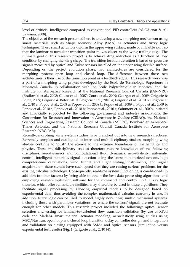
level of artificial intelligence compared to conventional PID controllers (Al-Odienat & Al-Lawama, 2008). The objective of the research presented here is to develop a new morphing mechanism using smart materials such as Shape Memory Alloy (SMA) as actuators and fuzzy logic techniques. These smart actuators deform the upper wing surface, made of a flexible skin, so that the laminar-to-turbulent transition point moves closer to the wing trailing edge. The ultimate goal of this research project is to achieve drag reduction as a function of flow condition by changing the wing shape. The transition location detection is based on pressure signals measured by optical and Kulite sensors installed on the upper wing flexible surface. Depending on the project evolution phase, two architectures are considered for the morphing system: open loop and closed loop. The difference between these two architectures is their use of the transition point as a feedback signal. This research work was a part of a morphing wing project developed by the Ecole de Technologie Supérieure in Montréal, Canada, in collaboration with the Ecole Polytechnique in Montréal and the Institute for Aerospace Research at the National Research Council Canada (IAR-NRC) (Brailovski et al., 2008; Coutu et al., 2007; Coutu et al., 2009; Georges et al., 2009; Grigorie & Botez, 2009; Grigorie & Botez, 2010; Grigorie et al., 2010 a; Grigorie et al., 2010 b; Grigorie et al., 2010 c; Popov et al., 2008 a; Popov et al., 2008 b; Popov et al., 2009 a; Popov et al., 2009 b; Popov et al., 2010 a; Popov et al., 2010 b; Popov et al., 2010 c; Sainmont et. al., 2009), initiated and financially supported by the following government and industry associations: the Consortium for Research and Innovation in Aerospace in Quebec (CRIAQ), the National Sciences and Engineering Research Council of Canada (NSERC), Bombardier Aerospace, Thales Avionics, and the National Research Council Canada Institute for Aerospace Research (NRC-IAR). Recently, morphing wing system studies have branched out into new research directions.
Extremely complex and catalogued as inter- and multidisciplinary studies, morphing wing
studies continue to ‘push’ the science to the extreme boundaries of mathematics and
physics. These multidisciplinary studies therefore require knowledge of the following
disciplines: aerodynamics and computational fluid dynamics, aeroelasticity, automatic
control, intelligent materials, signal detection using the latest miniaturized sensors, high
computer-time calculations, wind tunnel and flight testing, instruments, and signal
acquisition -- these signals have such speed that they are raising serious problems for the
existing calculus technology. Consequently, real-time system functioning is conditioned (in
addition to other factors) by being able to obtain the best data processing algorithms and
employing easy-to-implement software for the command and control unit. Fuzzy logic
theories, which offer remarkable facilities, may therefore be used in these algortihms. They
facilitate signal processing by allowing empirical models to be designed based on
experimental data; thus avoiding the complex mathematical calculus currently in use. In
addition, fuzzy logic can be used to model highly non-linear, multidimensional systems,
including those with parameter variations, or where the sensors’ signals are not accurate
enough for other models. This research project included the following: optical sensor
selection and testing for laminar-to-turbulent flow transition validation (by use of XFoil
code and Matlab), smart material actuator modeling, aeroelasticity wing studies using
MSC/Nastran, open loop and closed loop transition delay controller design, and integration
and validation on a wing equipped with SMAs and optical sensors (simulation versus
experimental test results) (Fig. 1 (Grigorie et al., 2010 b)).
www.intechopen.com

New Applications of Fuzzy Logic Methodologies in Aerospace Field
255
A first phase of this project involved the determination of optimized airfoils available for 35 different flow conditions expressed in terms of five Mach numbers (0.2, 0.225, 0.25, 0.275, 0.3) and seven angles of attack (-1˚, -0.5˚, 0˚, 0.5˚, 1˚, 1.5˚, 2˚) combinations. The optimized airfoils, derived from a laminar WTEA-TE1 reference airfoil, were calculated and used as a starting point in the actuation system design. Three steps were completed in the actuation system design phase: optimization of the number and positions of flexible skin actuation points, establishment of each actuation line’s architecture, and modeling of the smart materials actuators used in this application with fuzzy logic techniques. The next phase of the project was about the design of the actuation control, for which a fuzzy PD architecture was chosen. In this design, numerical simulations of the open loop morphing wing integrated system, based on an SMA non-linear model, were performed. As subsequent validation methods, a bench test and a wind tunnel test were conducted.
Actuationlines
Cavities forinstrumentation
Flexible skin(morphed extrados)
Rigidintrados
Rigid part ofthe extrados
Support plate foractuation system
Leadingedge
Trailingedge
Fig. 1. General architecture of the mechanical model
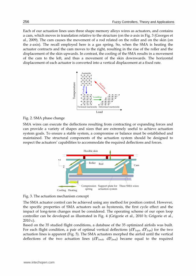
The shape memory actuator wires were made of nickel-titanium, known as Nitinol, and they contract as muscles do when electrically driven. This ability to flex or shorten is a characteristic of certain alloys that dynamically change their internal structure at certain temperatures. These alloys have the properties of exhibiting martensitic transformation when they deform at a low temperature phase, and may recover their original shape after heating (Popov et al., 2008 a). This phase change, from martensite to austenite, is shown in Fig. 2 (Baron et al., 2003; Thill et al., 2008). The load changes the internal forces between the atoms, forcing them to change their positions in the crystals and consequently forcing the wires to lengthen, which is called the SMA activation or the initial phase. When the wire is heated using a current, the heat generated by the current resistivity causes the atoms in the crystalline structure to realign and force the alloy to recover its original shape. Therefore, any change in the alloy’s internal temperature would modify the crystalline structure accordingly and thus the wire’s exterior shape. This property of changing the wire length as a function of the electrical current passing through the wire is used for actuation purposes (Popov et al., 2008 a). Another major reason for using Nitinol is that it is the most effective material at withstanding repeated cycles of heating and cooling without exhibiting a fatigue phenomenon (Gonzalez, 2005). SMA wires can process the deflections obtained using the applied forces and they provide a variety of shapes and sizes that are extremely useful to achieve actuation system goals. For example, SMA wires can provide high forces corresponding to small strains to achieve the correct balance between the forces and the deformations, as required by the actuation system. To ensure a stable system, a compromise or balance must be established and maintained. The structural components of the actuation system should be designed to respect the actuators’ capabilities to accommodate the required deflections and forces.
www.intechopen.com
Fuzzy Controllers, Theory and Applications
256
Each of our actuation lines uses three shape memory alloys wires as actuators, and contains a cam, which moves in translation relative to the structure (on the x-axis in Fig. 3 (Georges et al., 2009). The cam causes the movement of a rod related on the roller and on the skin (on the z-axis). The recall employed here is a gas spring. So, when the SMA is heating the actuator contracts and the cam moves to the right, resulting in the rise of the roller and the displacement of the skin upwards. In contrast, the cooling of the SMA results in a movement of the cam to the left, and thus a movement of the skin downwards. The horizontal displacement of each actuator is converted into a vertical displacement at a fixed rate.
Load
Tem
per
atu
re
Deformed martensiteTwinned martensite
Austenite
Loading
Co
oli
ng
Heating
Fig. 2. SMA phase change
SMA wires can execute the deflections resulting from contracting or expanding forces and can provide a variety of shapes and sizes that are extremely useful to achieve actuation system goals. To ensure a stable system, a compromise or balance must be established and maintained. The structural components of the actuation system should be designed to respect the actuators’ capabilities to accommodate the required deflections and forces.
HeatingCooling
Three SMA wires
Flexible skin
CamRoller
Support plate foractuation system
Rod
Compressionspring
x
z
Fig. 3. The actuation mechanism concept
The SMA actuator control can be achieved using any method for position control. However, the specific properties of SMA actuators such as hysteresis, the first cycle effect and the impact of long-term changes must be considered. The operating scheme of our open loop controller can be developed as illustrated in Fig. 4 (Grigorie et al., 2010 b; Grigorie et al., 2010 c). Based on the 35 studied flight conditions, a database of the 35 optimized airfoils was built. For each flight condition, a pair of optimal vertical deflections (dY1opt, dY2opt) for the two actuation lines is apparent (Fig. 5). The SMA actuators morphed the airfoil until the vertical deflections of the two actuation lines (dY1real, dY2real) became equal to the required
www.intechopen.com

New Applications of Fuzzy Logic Methodologies in Aerospace Field
257
α, M,Re
Pilot
Control
Flightconditions
Optimisedairfoils
databasedY
1opt
dY2opt
Real airfoil
Controller
dY1real
dY2real
SMAactuators
e=dYopt- dYreal
Airflowperturbations
Current
Positiontransducers
dY1real
dY2real
Fig. 4. Operating scheme of the SMA actuators’ control
deflections (dY1opt, dY2opt). The vertical deflections of the real airfoil at the actuation points were measured using two position transducers. The controller’s role is to send a command to supply an electrical current signal to the SMA actuators, based on the error signals (e) between the required vertical displacements and the obtained displacements. The designed controller was valid for both actuation lines, which are practically identical.
alpha1
alpha2
alpha3
alpha4
alpha5
alpha6
alpha7
0.2 0.22 0.24 0.26 0.28 0.3 0.32 0.34 0.362
3
4
5
6
7
8
Mach number
dY1
[mm
]
Mach number
dY2
[mm
]
2
3
4
5
6
7
8
0.2 0.22 0.24 0.26 0.28 0.3 0.32 0.34 0.36
Fig. 5. dY1opt and dY1opt, dY2opt as functions of M for various angles of attack
During the first phase of the controller design, numerical simulation of the controlled actuation system was performed; a step which required an SMA actuator model. In the literature, the modeling and control of smart material actuators can be categorized as recent research fields. Technical literature is available in three independent domains: modeling, control and smart materials. A smart actuator is formulated for a large range of smart materials and devices, and can be found in a variety of different configurations. It is common knowledge that all physical systems, including smart actuators, contain nonlinearities. As a consequence, linear modeling of smart material actuators may contain errors, while non-linear modeling remains possible. In order to conceive such a model, a fuzzy set must be designed, which may be given by the original fuzzy logic theory conceived by Lotfi A. Zadeh (Zadeh, 1965). The most serious problem arises from the determination of a complete set of rules and the membership functions corresponding to each input. The multiple attempts required to reduce errors and to optimize the model are time-consuming and, very often, the results are far from what was expected. A modern design method allows fuzzy model design to be completed in a relatively short time interval. The Adaptive Neuro-Fuzzy Inference System (ANFIS) design technique allows the generation and the optimization of the set of rules and the membership functions’ parameters by use of Neural Networks. Moreover, the ANFIS design technique already implemented in Matlab’s Neuro-Fuzzy software tools should be relatively easy to use.
www.intechopen.com

Fuzzy Controllers, Theory and Applications
258
Considering the numerical values resulting from the SMA experimental testing (forces, currents, temperatures and elongations), an empirical model can be developed, based on a neuro-fuzzy network. The model can learn the process behavior based on the input-output process data by using a Fuzzy Inference System (FIS), which should model the experimental data.
2. SMA actuator fuzzy model
The general aim of the SMA model is to calculate the elongation of the actuator (Δδ) under the application of a thermo-electro-mechanical load for some time (Δt). The load is so-qualified because the actuator can be operated by varying temperature (Tamb), by injection of electric current (i) or by applying a force (F). The geometry of the actuator is an SMA wire with constant section and perimeter over the length of the actuator. For these specific model objectives, in the first phase, the SMA actuators were experimentally tested in conditions close to those in which they will be used. The SMA testing was performed using at Tamb=24˚C, for six load cases with the forces of 700 N, 850 N, 1000 N, 1100 N, 1250 N and 1500 N. The electrical currents following the increasing-constant-decreasing-zero values evolution were applied to the SMA actuator for each of the six load cases. In each case, the following parameters were registered: time, the electrical current supplied to the SMA, the load force, the material temperature and the actuator elongation. To model the SMA we will built an integrated controller based on Adaptive Neuro-Fuzzy Inference Systems. The experimental elongation-current curves obtained from the six load cases are indicated in Fig. 6. One can observe that all six of the curves are characterized by four distinct zones: electrical current increase, constant electrical current, electrical current decrease and null electrical current in the cooling phase of the actuator. Therefore, four Fuzzy Inference Systems (FIS’s) are used to obtain four neuro-fuzzy controllers: one controller for the current increase, one for a constant current, one for the current decrease, and one controller for the null current (after its decrease). For the first and the third controllers, inputs such as the force and the current are used, while for the second and the fourth controller, inputs such as the force and the time values reflecting the SMA thermal inertia are used (for the four controllers the time values used are those required for the SMA to recover its initial temperature value (approximately 24˚C)). Finally, the four obtained controllers must be integrated into a single controller. The reasoning behind the design of the first and the third controllers is that from the available experimental data, two elongations for the same values of forces and currents are used (see Fig. 6). Due to the experimental data values, this data cannot be represented as algebraic functions, and therefore it is impossible to use the same FIS representation. An interpolation between the two elongation values obtained for the same values of forces and currents can be performed in Matlab, but it is not valid for our application. Also, the constant values, respectively the null values of the current before, respectively after the current decrease phase are not suggestive to be considered like inputs in the second and in the four controllers. Practically, with these phases the values of the actuator temperature could be used. The time values for these phases do prove very useful, because these values represent a measure of the thermal inertia of the actuator. We use the time value as the second input of the third controller, and therefore, as the second input of the second and of the fourth controllers – since force was considered as the first input (the time values must be considered from the moment when the current becomes constant, or null).
www.intechopen.com

New Applications of Fuzzy Logic Methodologies in Aerospace Field
259
700 N
850 N
1000 N
1100 N
1250 N
1500 N
0
5
10
15
20
25
30
Elo
ng
atio
n [
mm
]
Current [A]0 2 4 6 8 10 12
Fig. 6. Elongation versus the current values for different forces values for six load cases
2.1 SMA model architecture based on fuzzy logic controllers A fuzzy inference system (FIS) can be easily generated using Matlab’s “genfis1” or “genfis2” functions. The “genfis1” function generates a single-output Sugeno-type fuzzy inference system (FIS) using a grid partition on the data (no clustering). The FIS thus obtained is used to provide the initial conditions for ANFIS training. The “genfis1” function uses generalized bell-type membership functions for each input. Each rule generated by a “genfis1” function has one output membership function, which is a linear type by default. It is also possible to create the FIS using the Matlab “genfis2” function, which first generates an initial Sugeno-type FIS by decomposition of the operation domain into different regions using the fuzzy subtractive clustering method. For each region, a low order linear model can describe the local process parameters. The non-linear process can then be locally linearized around a functioning point by using the Least Squares method. The obtained model is considered valid in the entire region around this point. To limit the operating regions implies the existence of overlapping among these different regions, whose definition is given in a fuzzy manner. Thus, for each model input, several fuzzy sets are associated with their corresponding definitions of their membership functions. By combining these fuzzy inputs, the input space is divided into fuzzy regions. For each such region, a local linear model is used, while the global model is obtained by defuzzification with the center-of-gravity method (Sugeno), which interpolates the local models’ outputs (Sivanandam et al., 2007; MathWorks Inc., 2008). Based on the concept of finding regions with a high density of data points in the feature
space, the subtractive clustering method divides space into a number of clusters. Centers of
clusters are selected, starting with the points with the highest number of neighbours. The
clusters are identified one by one; for each cluster the data points within a prespecified
fuzzy radius are removed (subtracted). After each cluster identification, the algorithm looks
for a new one until all of the data points have been examined. If a collection of M data
points, specified by l-dimensional vectors uk, k = 1, 2..., M, is considered, a density measure
at data point uk can be defined as follows:
∑= ⎟⎟⎠
⎞⎜⎜⎝⎛ −−=ρ M
j m
jk
k r
uu
12
.)2/(
exp (1)
www.intechopen.com

Fuzzy Controllers, Theory and Applications
260
where rm is a positive constant that defines the radius within the fuzzy neighborhood and contributes to the density measure. The point with the highest density is selected as the first cluster center. Let uc1 be the point selected and ┩c1 its density measure. Next, the density measure for each data point uk is revised by the formula:
.)2/(
exp2
1
1 ⎟⎟⎠⎞
⎜⎜⎝⎛ −−ρ−ρ=ρ′
n
ck
ckk r
uu (2)
in which rn is a positive constant, larger than rm, and defines a neighborhood to be reduced in its density measure to prevent closely-spaced cluster centers. In this way, the data points near the first cluster center uc1 will have significantly reduced density measures, and these points cannot be selected as centers for the next clusters. After the density measure for each point has been revised, the next cluster center uc2 is selected and all the density measures are revised again. The process is repeated until all of the data points have been examined and a sufficient number of cluster centers generated. When the subtractive clustering method is applied to an input-output data set, each of the cluster centers are used as the centers for the premise sets in a singleton type of rule base (Khezri & Jahed, 2007). The Matlab “genfis1” function generates membership functions of a generalized bell type, defined as follows (Kosko, 1992; Kung & Su, 2007):
,)|/)(|1()( 12 −−+= bi
q
i
q acxxA (3)
where i
qc is the cluster center defining the position of the membership function, a, b are two
parameters which define the shape of the membership function, and ),1( NiA i
q = are
associated individual antecedent fuzzy sets of each input variable (N - number of rules). The Matlab “genfis2” function generates membership functions of the Gaussian type, described by the following expression (Kosko, 1992; Kung & Su, 2007):
},)/)((5.0exp{)( 2i
q
i
q
i
q cxxA σ−−= (4)
where i
qc is the cluster center, and i
qσ is the dispersion of the cluster. The Sugeno fuzzy model was proposed by Takagi, Sugeno and Kang to generate the fuzzy rules from a given input-output data set (Mahfouf et al., 1999). For our system, for all four of the FIS’s (two inputs and one output) a first-order model is considered, and for N rules is given by (Kung & Su, 2007; Mahfouf et al., 1999):
,),(then,isandisIf:Rule
,),(then,isandisIf:Rule
,),(then,isandisIf:1Rule
22110212211
22110212211
2
1
21
1
1
1
021
11
22
1
11
xaxabxxyAxAxN
xaxabxxyAxAxi
xaxabxxyAxAx
NNNNNN
iiiiii
++=++=++=
B
B (5)
where )2,1( =qxq are individual input variables, and ),1( Niy i = is the first-order
polynomial function in the consequent. ),1,2,1( Nikai
k == are the parameters of the linear
function and ),1(0
Nibi = denotes a scalar offset. The parameters ),1,2,1(,0
Nikba ii
k == are
optimized by Least Square method.
www.intechopen.com

New Applications of Fuzzy Logic Methodologies in Aerospace Field
261
For any input vector, Txx ],[21
=x , if the singleton fuzzifier, the product fuzzy inference and
the center-average defuzzifier are applied, the output of the fuzzy model y is inferred as follows (weighted average):
,)(/)(11
⎟⎠⎞⎜⎝
⎛⎟⎠⎞⎜⎝
⎛= ∑∑==
N
i
iN
i
ii wywy xx (6)
where
).()()(2211
xAxAw iii ×=x (7)
)(xiw represents the degree of fulfillment of the antecedent, that is, the level of firing of the
ith rule. The adaptive neuro-fuzzy inference system adapts the parameters of Sugeno-type fuzzy inference systems using the neural networks. A very simple way to realize the FIS’s training is by using the Matlab “ANFIS” function, which use a learning algorithm for the identification of the membership functions’ parameters of a Sugeno-type fuzzy inference system with two outputs and one input. As a starting point, the input-output data and the FIS models generated with the “genfis1” or “genfis2” functions are considered. The “ANFIS” optimizes the membership functions’ parameters for a number of training epochs; this number is set by the user. The optimization is realized for a better process approximation performed by the neuro-fuzzy model by means of a quality parameter present in the training algorithm (MathWorks Inc., 2008). Following the training phase, the models may be used for elongation value generation corresponding to the parameters at the input. For training the fuzzy system, ANFIS employs a back-propagation algorithm for the parameters associated with the input membership functions, and a least mean square estimation for the parameters associated with the output membership functions. For the FISs generated using the “genfis1” or “genfis2” functions, the membership functions are of the generalized bell type and gaussian type, respectively. In accordance with equations (3) and (4), in these kinds of membership functions, a, b and c, and σ and c, respectively, are considered variables and must be adjusted. Therefore, the back-propagation algorithm may be used to train these parameters. In this way, we can achieve our goal to minimize a cost function of the form
( ) ,2/2yydes −=ε (8)
where ydes is desired output. The output of each rule ),(21
xxy i is defined by:
),/()()1( i
y
ii yktyty ∂ε∂−=+ (9)
in which ky is the step size. Starting from the Sugeno system’s output (eq. (6)), we find:
,ii y
y
yy ∂∂⋅∂
ε∂=∂ε∂
(10)
with
www.intechopen.com
Fuzzy Controllers, Theory and Applications
262
.)(/)(,1
∑=
=∂∂−=∂
ε∂ N
i
i
iides wwy
yyy
yxx (11)
Therefore, the following equation for the output of each rule is
.)(/)()()()1(1
∑=
⋅−⋅−=+ N
i
i
idesy
ii wwyyktyty xx (12)
If a generalized bell-type membership function is used, for the jth membership function of the ith fuzzy rule the parameters are determined with the relations:
.)()1(,)()1(,)()1(i
j
c
i
j
i
ji
j
b
i
j
i
ji
j
a
i
j
i
j cktctc
bktbtb
aktata ∂
ε∂−=+∂ε∂−=+∂
ε∂−=+ (13)
For a Gaussian-type membership function, the parameters of the jth membership function of the ith fuzzy rule are calculated with the relations:
)./()()1(),/()()1( i
jc
i
j
i
j
i
j
i
j
i
j cktctcktt ∂ε∂−=+σ∂ε∂−σ=+σ σ (14)
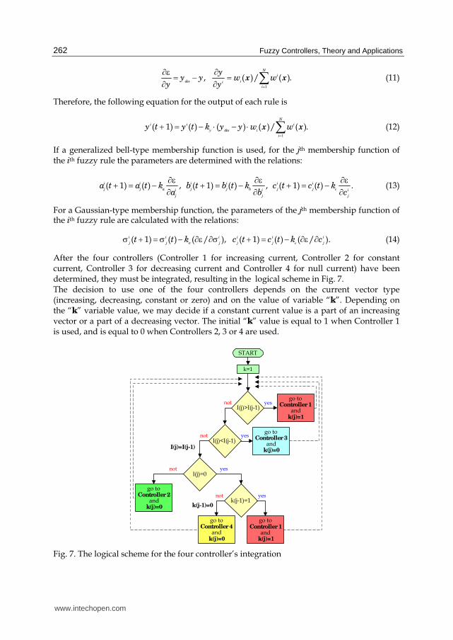
After the four controllers (Controller 1 for increasing current, Controller 2 for constant current, Controller 3 for decreasing current and Controller 4 for null current) have been determined, they must be integrated, resulting in the logical scheme in Fig. 7. The decision to use one of the four controllers depends on the current vector type (increasing, decreasing, constant or zero) and on the value of variable “k”. Depending on the “k” variable value, we may decide if a constant current value is a part of an increasing vector or a part of a decreasing vector. The initial “k” value is equal to 1 when Controller 1 is used, and is equal to 0 when Controllers 2, 3 or 4 are used.
k=1
I(j)>I(j-1)yesnot
I(j)<I(j-1)yesnot
I(j)=0
I(j)=I(j-1)
yes
k(j-1)=1yesnot
not
k(j-1)=0
go toController 1
andk(j)=1
go toController 1
andk(j)=1
go toController 4
andk(j)=0
START
go toController 3
andk(j)=0
go toController 2
andk(j)=0
Fig. 7. The logical scheme for the four controller’s integration
www.intechopen.com

New Applications of Fuzzy Logic Methodologies in Aerospace Field
263
2.2 The SMA model design and evaluation In a first phase, the “genfis2” Matlab function (MathWorks Inc., 2008) was used to generate
and train the FISs associated with the four controllers in Fig. 7: “Controller1Fis” (for the
increasing current phase), “Controller2Fis” (for the constant current phase),
“Controller3Fis” (for the decreasing current phase) and “Controller4Fis” (for the null values
of the current obtained after the decreasing phase).
The first FIS, with force and electrical current as its inputs, was trained for 5000 epochs
using the “ANFIS” Matlab function. The rules were of the type: if (in1 is in1cluster„k”) and
(in2 is in2cluster„k”) then (out1 is out1cluster„k”). For both of these inputs, nine Gaussian-
type membership functions (mf) were generated; within the set of rules they are noted by:
in„j”cluster„k”; where j is the input number (1÷2), and k is the number of the membership
function (1-9). “Controller1Fis” fuzzy inference system thus has the structure shown in Fig.
8, while Controller 1 has the structure indicated in Fig. 9.
The rules of “Controller1Fis” fuzzy inference system, before and after training, are
presented in Fig. 10, and Fig. 11 displays the deviation between the neuro-fuzzy models and
the experimentally obtained data, defining the quality parameter from the training
algorithm, for different training epochs.
Figure 11 shows a rapid decrease in the deviation between the experimental data and the
neuro-fuzzy model for the quality parameter within the training algorithm over the first 100
training epochs, from a value of 0.062 to 0.03. Evaluating the FIS before and after training for
the experimental data, using the “evalfis” command, the characteristics in Fig. 12 were
obtained. The mean of the relative absolute values of the errors decreased from 0.3063%
before training to 0.119% after training, while its maximum value decreased from 0.9339% to
0.4342%. Since the error determined for “Controller1Fis” was very small, this FIS was
selected to be implemented in the Simulink integrated controller.
Fig. 8. Structure of the “Controller1Fis” fuzzy inference system
www.intechopen.com

Fuzzy Controllers, Theory and Applications
264
in1Force
in2
out1
Elongation
Sugeno
FIS
Current
Fig. 9. The structure of Controller 1
Fig. 10. The “Controller1Fis” rules, before and after training
From Fig. 12 one observes a good overlapping of the FIS model with the elongation
experimental data. This superposition is dependent upon the training epochs’ number, and
improves as the number of training epochs increases. Because the training errors take
constant values, an improved approximation of the real model can be achieved with neuro-
fuzzy methods only in the case when a larger amount of experimental data is used.
0 500 1000 1500 2000 2500 3000 3500 4000 4500 5000
"Controller1Fis"
Number of training epochs
Dev
iati
on
0.025
0.03
0.035
0.04
0.045
0.05
0.055
0.06
0.065
Fig. 11. The training error for “Controller1Fis”
www.intechopen.com

New Applications of Fuzzy Logic Methodologies in Aerospace Field
265
"Controller1Fis" after training
Elo
ng
atio
n [
mm
]
Number of experimental data points
10
12
14
16
18
20
22
24
26
0 10 20 30 40 50 60
data
FIS model
F=700N
F=850N
F=1000N
F=1100N
F=1250N
F=1500N
"Controller1Fis" before training
Elo
ng
atio
n [
mm
]
Number of experimental data points
10
12
14
16
18
20
22
24
26
0 10 20 30 40 50 60
data
FIS model
F=700N
F=850N
F=1000N
F=1100N
F=1250N
F=1500N
0 2 4 6 8 10 12Current [A]
data
FIS model
Elo
ng
atio
n [
mm
]
10
12
14
16
18
20
22
24
26"Controller1Fis" before training
F=700N
F=850N
F=1000N
F=1100N
F=1250N
F=1500N
0 2 4 6 8 10 12Current [A]
data
FIS modelE
lon
gat
ion
[m
m]
10
12
14
16
18
20
22
24
26"Controller1Fis" after training
F=700N
F=850N
F=1000N
F=1100N
F=1250N
F=1500N
Fig. 12. “Controller1Fis” evaluation, before and after training
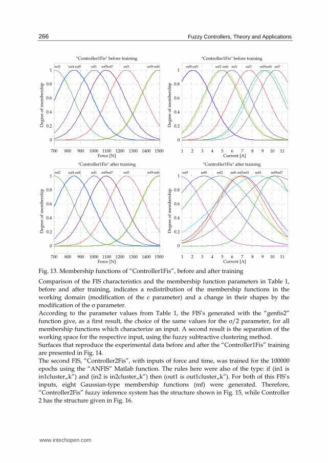
The parameters of the input’s membership functions for “Controller1Fis”, before and after
training, are shown in Table 1, while the membership functions’ shapes are depicted in Fig.
13. For the Gaussian-type membership functions generated with “genfis2”, the parameters
are half of the dispersion (σ/2) and the center for the membership function (c).
Status Input Param. mf1 mf2 mf3 mf4 mf5 mf6 mf7 mf8 mf9
σ/2 142.7 142.7 142.7 142.7 142.7 142.7 142.7 142.7 142.7 Force [N] c 1003 701.6 1248 851.8 1096 1493 1094 849.3 1498
σ/2 1.867 1.867 1.867 1.867 1.867 1.867 1.867 1.867 1.867
Before training Current
[A] c 6 4.95 7.7 9.45 2.08 5.1 10.4 2.1 9.18
σ/2 142.8 142.8 142.7 142.7 142.7 142.7 142.7 142.7 142.8 Force [N] c 1003 701.6 1248 851.8 1096 1493 1094 849.4 1498
σ/2 2.598 3.321 2.328 4.208 2.271 2.252 3.671 2.965 1.885
After training Current
[A] c 6.998 4.795 6.942 8.627 0.7952 6.609 10.35 3.194 10.21
Table 1. Parameters of the “Controller1FIS” input’s mf, before and after training
www.intechopen.com
Fuzzy Controllers, Theory and Applications
266
Deg
ree
of
mem
ber
ship
mf1mf2 mf3mf4 mf5 mf6mf7mf8 mf9
Force [N]700 800 900 1000 1100 1200 1300 1400 1500
0
0.2
0.4
0.6
0.8
1
"Controller1Fis" before training
Deg
ree
of
mem
ber
ship
mf1mf2 mf3mf4 mf5 mf6mf7mf8 mf9
Force [N]700 800 900 1000 1100 1200 1300 1400 1500
0
0.2
0.4
0.6
0.8
1
"Controller1Fis" after training
mf1mf2 mf3 mf4mf5 mf6 mf7mf8 mf9
1 2 3 4 5 6 7 8 9 10 11
Deg
ree
of
mem
ber
ship
Current [A]
0
0.2
0.4
0.6
0.8
1
"Controller1Fis" before training
mf3mf1mf2 mf4mf5 mf6 mf7mf8 mf9
1 2 3 4 5 6 7 8 9 10 11
Deg
ree
of
mem
ber
ship
Current [A]
0
0.2
0.4
0.6
0.8
1
"Controller1Fis" after training
Fig. 13. Membership functions of “Controller1Fis”, before and after training
Comparison of the FIS characteristics and the membership function parameters in Table 1,
before and after training, indicates a redistribution of the membership functions in the
working domain (modification of the c parameter) and a change in their shapes by the
modification of the σ parameter.
According to the parameter values from Table 1, the FIS’s generated with the “genfis2”
function give, as a first result, the choice of the same values for the σ/2 parameter, for all
membership functions which characterize an input. A second result is the separation of the
working space for the respective input, using the fuzzy subtractive clustering method.
Surfaces that reproduce the experimental data before and after the “Controller1Fis” training
are presented in Fig. 14.
The second FIS, “Controller2Fis”, with inputs of force and time, was trained for the 100000
epochs using the “ANFIS” Matlab function. The rules here were also of the type: if (in1 is
in1cluster„k”) and (in2 is in2cluster„k”) then (out1 is out1cluster„k”). For both of this FIS’s
inputs, eight Gaussian-type membership functions (mf) were generated. Therefore,
“Controller2Fis” fuzzy inference system has the structure shown in Fig. 15, while Controller
2 has the structure given in Fig. 16.
www.intechopen.com

New Applications of Fuzzy Logic Methodologies in Aerospace Field
267
8001000
12001400
24
68
10
Force [N]
"Controller1Fis" before training
Current [A]
12
14
16
18
20
22
24
Elo
ng
ati
on
[m
m]
8001000
12001400
24
68
10
Force [N]Current [A]
12
14
16
18
20
22
24
Elo
ng
atio
n [
mm
]
"Controller1Fis" after training
Fig. 14. Control surfaces resulted for “Controller1Fis”, before and after training
Fig. 15. Structure of the “Controller2Fis” fuzzy inference system
in1Force
in2
out1
Elongation
Sugeno
FIS
Time
Fig. 16. The structure of Controller 2
The rules of the “Controller2Fis” fuzzy inference system, before and after training, are
presented in Fig. 17, while Fig. 18 displays the deviation between the neuro-fuzzy models
and the experimentally obtained data, defining the quality parameter from the training
algorithm, for different training epochs.
www.intechopen.com

Fuzzy Controllers, Theory and Applications
268
Fig. 17. The “Controller2Fis” rules, before and after training
"Controller2Fis"
Number of training epochs
Dev
iati
on
0.05
0.1
0.15
0.2
0.25
0.3
0.35
0.4
0 1 2 3 4 5 6 7 8 9 10
x 104
Fig. 18. The training error for “Controller2Fis”
Figure 18 shows a rapid decrease in the deviation between the experimental data and the neuro-fuzzy model for the quality parameter within the training algorithm over the first 5000 training epochs, from 0.31 until a value of 0.09. Evaluating the FIS before and after training for the experimental data, the characteristics in Fig. 19 were obtained. The mean of the relative absolute values of the errors decreased by 3.76 times -- from 3.3503% before training to 0.8902% after training. Considering that the error for the “Controller2Fis” is in the desired limits after 100000 training epochs, this FIS was selected to be implemented in the Simulink integrated controller. In Fig. 19, a good overlapping of the FIS models’ data with the elongation experimental data is clearly visible. As in the previous FIS case, this superposition is dependent on the training epochs’ number, and improves as the number of training epochs increases. The parameters of the input’s membership functions for the “Controller2Fis”, before and after training, are shown in Table 2, while the membership functions’ shapes are depicted in Fig. 20. Comparison of the FIS characteristics and the membership functions parameters, before and after training, indicates a redistribution of the membership functions in the working domain
www.intechopen.com

New Applications of Fuzzy Logic Methodologies in Aerospace Field
269
(modification of the c parameter) and a change in their shapes by modification of the σ parameter (Table 2).
Elo
ng
atio
n [
mm
]
0
5
10
15
20
25
Time [s]
data
FIS model
"Controller2Fis" after training
F=700N
F=850NF=1000N
F=1100N
F=1250N
F=1500N
0 5 10 15 20 25 300 50 100 150 200 250 300
Elo
ng
atio
n [
mm
]
Number of experimental data points
F=700N
F=850N
F=1000N
F=1100N
F=1250N
F=1500N
"Controller2Fis" after training
0
5
10
15
20
25
data
FIS model
0
5
10
15
20
25
30
Time [s]
data
FIS model
Elo
ng
atio
n [
mm
]
"Controller2Fis" before training
F=700N
F=850N
F=1000N
F=1100N
F=1250N
F=1500N
0 5 10 15 20 25 300
5
10
15
20
25
30data
FIS model
0 50 100 150 200 250 300
Elo
ng
atio
n [
mm
]
Number of experimental data points
F=700N
F=850N
F=1000N
F=1100N
F=1250N
F=1500N
"Controller2Fis" before training
Fig. 19. “Controller2Fis” evaluation, before and after training
Status Input Param. mf1 mf2 mf3 mf4 mf5 mf6 mf7 mf8
σ/2 143 143 143 143 143 143 143 143 Force [N]
c 1002 1254 700.9 1096 1503 1002 1492 699.5
σ/2 4.757 4.757 4.757 4.757 4.757 4.757 4.757 4.757
Before training
Time [s]c 11.86 8.412 10.46 21.75 13.06 2.355 2.968 1.562
σ/2 159.8 134.6 142.2 137.4 142.1 133.1 150.1 144.6 Force [N]
c 1007 1254 702.7 1099 1498 997.4 1487 700.3
σ/2 2.624 4.197 3.393 2.768 5.349 5.261 1.835 3.346
After training
Time [s]c 8.244 0.9308 8.639 11.89 6.099 -5.344 1.777 -3.61
Table 2. Parameters of the “Controller2FIS” input’s mf before and after training
www.intechopen.com

Fuzzy Controllers, Theory and Applications
270
mf1 mf2mf3 mf4 mf5mf6 mf7mf8
Deg
ree
of
mem
ber
ship
Force [N]700 800 900 1000 1100 1200 1300 1400 1500
0
0.2
0.4
0.6
0.8
1
"Controller2Fis" after training
mf1mf2 mf3 mf4mf5mf6 mf7mf8
0 5 10 15 20 25
Deg
ree
of
mem
ber
ship
Time [s]
0
0.2
0.4
0.6
0.8
1
"Controller2Fis" before training
mf1 mf2mf3 mf4 mf5mf6 mf7mf8
Deg
ree
of
mem
ber
ship
Force [N]700 800 900 1000 1100 1200 1300 1400 1500
0
0.2
0.4
0.6
0.8
1
"Controller2Fis" before training
mf1mf2 mf3 mf4mf5mf6 mf7mf8
0 5 10 15 20 25
Deg
ree
of
mem
ber
ship
Time [s]
0
0.2
0.4
0.6
0.8
1
"Controller2Fis" after training
Fig. 20. Membership functions of “Controller2Fis”, before and after training
Surfaces which reproduce the experimental data, before and after the “Controller2Fis” training, are represented in Fig. 21.
800
1000
1200
1400 05
1015
2025
5
10
15
20
25
Time [s]Force [N]
Elo
ng
atio
n [
mm
]
"Controller2Fis" before training "Controller2Fis" after training
800
10001200
14000
510
1520
25
10
15
20
25
Time [s]Force [N]
Elo
ng
atio
n [
mm
]
Fig. 21. Control surface resulted for “Controller2Fis”, before and after training
www.intechopen.com

New Applications of Fuzzy Logic Methodologies in Aerospace Field
271
The third FIS, “Controller3Fis”, which has the force and the current as its inputs, was
trained for 20.000 epochs. The rules were also of the type: if (in1 is in1cluster„k”) and (in2 is
in2cluster„k”) then (out1 is out1cluster„k”). For both of this FIS’s inputs, seven Gaussian-
type membership functions (mf) were generated. Therefore, “Controller3Fis” fuzzy
inference system has the structure presented in Fig. 22, while Controller 3 has the same
structure as Controller 1, represented in Fig. 9.
The rules of the “Controller3Fis” fuzzy inference system, before and after training, are
presented in Fig. 23, and Fig. 24 displays the deviation between the neuro-fuzzy models and
the experimentally obtained data for different training epochs, defining the quality
parameter from the training algorithm.
Fig. 22. Structure of the “Controller3Fis” fuzzy inference system
Fig. 23. The “Controller3Fis” rules, before and after training
www.intechopen.com

Fuzzy Controllers, Theory and Applications
272
Figure 24 shows a decrease in the deviation between the experimental data and the neuro-
fuzzy model for the quality parameter (with some oscillations) within the training algorithm
over the first 3500 training epochs, from the value of 2.52·10-4 to that of 2.05·10-4. Evaluating
the FIS before and after training for the experimental data, the characteristics in Fig. 25 were
obtained. The mean of the relative absolute values of the errors decreased from 1.5154·10-3 %
before training, to 2.3106·10-13 % after training. “Controller3Fis” was selected to be
implemented in the Simulink integrated controller because its obtained error was within the
desired limits after 20000 training epochs.
From Fig. 25 one observes a good overlapping of the FIS models with the elongation
experimental data. As in the previous FISs cases, this superposition is dependent upon the
training epochs’ number, and is better as the number of training epochs is higher.
Number of training epochs
Dev
iati
on
x 10-4
1.7
1.8
1.9
2
2.1
2.2
2.3
2.4
2.5
2.6
0 0.2 0.4 0.6 0.8 1 1.2 1.4 1.6 1.8 2
x 104
"Controller3Fis"
Fig. 24. The training error for “Controller3Fis”
The parameters of the input’s membership functions for “Controller3Fis”, before and after training, are shown in Table 3, while the membership functions’ shapes are depicted in Fig. 26.
Status Input Param. mf1 mf2 mf3 mf4 mf5 mf6 mf7
σ/2 141.8 141.8 141.8 141.8 141.8 141.8 141.8 Force [N]
c 1003 847.3 1102 701 1250 1497 1500
σ/2 2.042 2.042 2.042 2.042 2.042 2.042 2.042
Before training Current
[A] c 0 11.55 11.44 0 0 10.2 0
σ/2 141.7 141.8 141.8 141.7 141.6 141.8 141.8 Force [N]
c 1003 847.3 1102 701 1250 1497 1500
σ/2 2.042 2.165 1.838 2.042 2.042 2.058 2.042
After training Current
[A] c 8.184·10-5 11.3 11.73 -1.398·10-6 -4.591·10-6 10.25 -1.582·10-7
Table 3. Parameters of the “Controller3FIS” input’s mf before and after training
www.intechopen.com
New Applications of Fuzzy Logic Methodologies in Aerospace Field
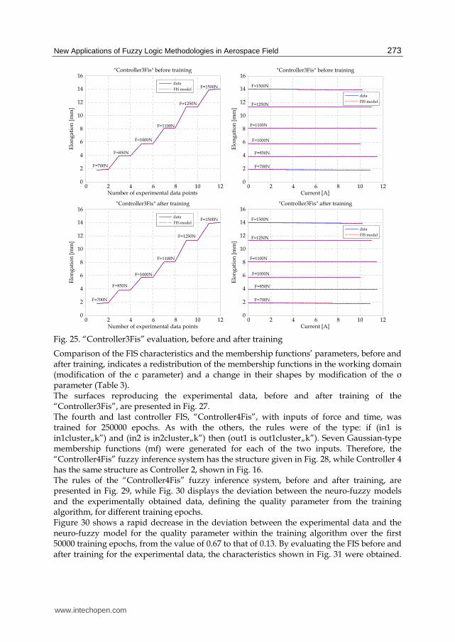
273
Elo
ng
ati
on
[m
m]
Number of experimental data points
F=700N
F=850N
F=1000N
F=1100N
F=1250N
F=1500N
"Controller3Fis" before training
0
2
4
6
8
10
12
14
16
0 2 4 6 8 10 12
data
FIS model
Elo
ng
atio
n [
mm
]
Current [A]
F=700N
F=850N
F=1000N
F=1100N
F=1250N
F=1500N
"Controller3Fis" before training
0
2
4
6
8
10
12
14
16
0 2 4 6 8 10 12
data
FIS model
Elo
ng
atio
n [
mm
]
Current [A]
F=700N
F=850N
F=1000N
F=1100N
F=1250N
F=1500N
"Controller3Fis" after training
0
2
4
6
8
10
12
14
16
0 2 4 6 8 10 12
data
FIS model
Elo
ng
atio
n [
mm
]
Number of experimental data points
F=700N
F=850N
F=1000N
F=1100N
F=1250N
F=1500N
"Controller3Fis" after training
0
2
4
6
8
10
12
14
16
0 2 4 6 8 10 12
data
FIS model
Fig. 25. “Controller3Fis” evaluation, before and after training
Comparison of the FIS characteristics and the membership functions’ parameters, before and after training, indicates a redistribution of the membership functions in the working domain (modification of the c parameter) and a change in their shapes by modification of the σ parameter (Table 3). The surfaces reproducing the experimental data, before and after training of the “Controller3Fis”, are presented in Fig. 27. The fourth and last controller FIS, “Controller4Fis”, with inputs of force and time, was trained for 250000 epochs. As with the others, the rules were of the type: if (in1 is in1cluster„k”) and (in2 is in2cluster„k”) then (out1 is out1cluster„k”). Seven Gaussian-type membership functions (mf) were generated for each of the two inputs. Therefore, the “Controller4Fis” fuzzy inference system has the structure given in Fig. 28, while Controller 4 has the same structure as Controller 2, shown in Fig. 16. The rules of the “Controller4Fis” fuzzy inference system, before and after training, are presented in Fig. 29, while Fig. 30 displays the deviation between the neuro-fuzzy models and the experimentally obtained data, defining the quality parameter from the training algorithm, for different training epochs. Figure 30 shows a rapid decrease in the deviation between the experimental data and the neuro-fuzzy model for the quality parameter within the training algorithm over the first 50000 training epochs, from the value of 0.67 to that of 0.13. By evaluating the FIS before and after training for the experimental data, the characteristics shown in Fig. 31 were obtained.
www.intechopen.com

Fuzzy Controllers, Theory and Applications
274
The mean of the relative absolute values of the errors decreased from 5.1855% before training, to 1.0316% after training. Since the error found for the “Controller4Fis” was within the desired limits after 250000 training epochs, this FIS was chosen to be implemented in the Simulink integrated controller.
mf1mf2 mf3mf4 mf5 mf6 mf7
Deg
ree
of
mem
ber
ship
Force [N]
0
0.2
0.4
0.6
0.8
1
"Controller3Fis" after training
700 800 900 1000 1100 1200 1300 1400
mf1 mf2 mf3mf4
mf5
mf6
mf7
0 2 4 6 8 10
Deg
ree
of
mem
ber
ship
Current [A]
0
0.2
0.4
0.6
0.8
1
"Controller3Fis" after training
mf1 mf2mf3mf4
mf5
mf6
mf7
0 2 4 6 8 10
Deg
ree
of
mem
ber
ship
Current [A]
0
0.2
0.4
0.6
0.8
1
"Controller3Fis" before training
mf7mf1mf2 mf3mf4 mf5 mf6
Deg
ree
of
mem
ber
ship
Force [N]
0
0.2
0.4
0.6
0.8
1
"Controller3Fis" before training
700 800 900 1000 1100 1200 1300 1400
Fig. 26. Membership functions of “Controller3Fis”, before and after training
8001000
12001400
0
5
10
Force [N]
Current [A]
Elo
ng
atio
n [
mm
]
"Controller3Fis" after training
0
5
10
15
20
Force [N]
Current [A]
Elo
ng
atio
n [
mm
]
8001000
12001400
0
5
10
-5
0
5
10
15
20
"Controller3Fis" before training
Fig. 27. Control surface resulted for “Controller3Fis”, before and after training
www.intechopen.com

New Applications of Fuzzy Logic Methodologies in Aerospace Field
275
Fig. 28. Structure of the “Controller4Fis” fuzzy inference system
Fig. 29. Rules of the “Controller4Fis” before and after training
"Controller4Fis"
Dev
iati
on
0.1
0.2
0.3
0.4
0.5
0.6
0.7
0.8
0 0.5 1 1.5 2 2.5
x 105
Number of training epochs
Fig. 30. The “Controller4Fis” training error
www.intechopen.com

Fuzzy Controllers, Theory and Applications
276
0 50 100 1500
5
10
15
20
25
30
Time [s]
data
FIS modelE
lon
gat
ion
[m
m]
"Controller4Fis" after training
F=700N
F=850N
F=1000N
F=1100N
F=1250N
F=1500N
0 50 100 1500
5
10
15
20
25
30
Time [s]
data
FIS model
Elo
ng
atio
n [
mm
]
"Controller4Fis" before training
F=700N
F=850N
F=1000N
F=1100N
F=1250N
F=1500N
0
5
10
15
20
25
30
Elo
ng
atio
n [
mm
]
Number of experimental data points
F=700N
F=850N
F=1000N
F=1100N
F=1250N
F=1500N
"Controller4Fis" after training
0 200 400 600 800 1000 1200 1400
data
FIS model
0
5
10
15
20
25
30
Elo
ng
atio
n [
mm
]
Number of experimental data points
F=700N
F=850N
F=1000N
F=1100N
F=1250N
F=1500N
"Controller4Fis" before training
0 200 400 600 800 1000 1200 1400
data
FIS model
Fig. 31. “Controller4Fis” evaluation, before and after training
From Fig. 31, a good overlapping of the FIS model’s output with the elongation experimental data can be observed. As in the previous FIS cases, this superposition is dependent upon the training epochs’ number, and is better as the number of training epochs is higher. The parameters of the input’s membership functions for the “Controller4Fis”, before and after training, are shown in Table 4, while the membership functions’ shapes are depicted in Fig. 32.
Status Input Param. mf1 mf2 mf3 mf4 mf5 mf6 mf7
σ/2 143.4 143.4 143.4 143.4 143.4 143.4 143.4 Force [N]
c 1003 847 1255 703 1103 1505 1497
σ/2 24.86 24.86 24.86 24.86 24.86 24.86 24.86
Before training
Time [s] c 26.03 92.38 53.75 33.43 112.2 54.45 12.09
σ/2 131.2 154.4 119 107.7 148.2 142.7 216.1 Force [N]
c 975.6 862 1309 747.9 1077 1493 1462
σ/2 15.24 13.58 11.41 13.16 13.71 10.4 16.79
After training
Time [s] c 59.28 64.99 51.19 54.08 76.06 50.11 44.6
Table 4. Parameters of the“Controller4FIS” input’s mf before and after training
www.intechopen.com

New Applications of Fuzzy Logic Methodologies in Aerospace Field
277
mf1mf2mf3mf4
mf5mf6
mf7
0 20 40 60 80 100 120 140
Deg
ree
of
mem
ber
ship
Time [s]
0
0.2
0.4
0.6
0.8
1
"Controller4Fis" after training
mf1mf2 mf3mf4 mf5 mf6mf7
Deg
ree
of
mem
ber
ship
Force [N]700 800 900 1000 1100 1200 1300 1400 1500
0
0.2
0.4
0.6
0.8
1
"Controller4Fis" after training
mf1 mf2mf3mf4 mf5mf6mf7
0 20 40 60 80 100 120 140
Deg
ree
of
mem
ber
ship
Time [s]
0
0.2
0.4
0.6
0.8
1
"Controller4Fis" before training
mf1mf2 mf3mf4 mf5 mf6mf7
Deg
ree
of
mem
ber
ship
Force [N]700 800 900 1000 1100 1200 1300 1400 1500
0
0.2
0.4
0.6
0.8
1
"Controller4Fis" before training
Fig. 32. Membership functions of “Controller4Fis”, before and after training
Comparison of the FIS characteristics and the membership functions parameters, before and after training, indicates a redistribution of the membership functions in the working domain (modification of the c parameter) and a change in their shapes by the modification of the σ parameter (Table 4). The surfaces reproducing the experimental data, before and after training of the “Controller4Fis”, are presented in Fig. 33.
8001000
12001400
0
50
100
Time [s]
Force [N]
Elo
ng
atio
n [
mm
]
"Controller4Fis" before training
5
10
15
20
25
30
35
8001000
12001400
0
50
100
"Controller4Fis" after training
Elo
ng
atio
n [
mm
]
5
10
15
20
25
30
Time [s]
Force [N]
Fig. 33. Control surface resulted for “Controller4Fis”, before and after training
www.intechopen.com

Fuzzy Controllers, Theory and Applications
278
Each of the four obtained FISs was imported at the fuzzy controller level, resulting in four controllers: Controller 1 (“Controller1Fis”), Controller 2 (“Controller2Fis”), Controller 3 (“Controller3Fis”), and Controller 4 (“Controller4Fis”). The integration of these four controllers is carried out using the logical scheme given in Fig. 7; resulting in the Matlab/Simulink model below, in Fig. 34.
Current
Force
Elongation
variable " k "
C is the maximum time for the actuator
to recover its initial temperature
if the current becomes null
Te is the sample time
in the experimental data
T is the value of the sample time
for simulation
El
To Workspace
Switch7 Switch6
Switch5
Switch4
Switch3
Switch2
Switch1
Switch
Current
Signal FromWorkspace1
Force
Signal FromWorkspace
AND
LogicalOperator3
NOT
LogicalOperator2
AND
LogicalOperator1
1s
Integrator2
1s
Integrator1
T/Te
Gain2
T/Te
Gain1Fuzzy LogicController 4
Fuzzy LogicController 3
Fuzzy LogicController 2
Fuzzy LogicController 1
U > U/z
DetectIncrease
U < U/z
DetectDecrease1
z
1
C
Constant6
1
Constant5
0
Constant4
0
Constant3
1
Constant2
0
Constant1
1
Constant
== 0
CompareTo Zero1
== 0
CompareTo Zero
Fig. 34. The integration model schema in Matlab/Simulink
In the Matlab/Simulink model shown in Fig. 34, the second input for Controller 2 and for Controller 4 (Time) is generated by using an integrator, and starts from the moment that either of these controllers is used (the input of the Gain block is 0 if the schema decides not to work with either Controller 2 or 4). Because is possible that the simulation sample time may be different than the sample time used in the experimental data acquisition process, we use the “Gain” block that gives their rapport; “Te” is the sample time in the experimental data and “T” is the simulation sample time. In the scheme, the constant “C” represents the maximum time that it takes for the actuator to recover its initial temperature (approximately 24˚C) when the current becomes null. Evaluating the integrated model for controller (Fig. 34) in all six cases of experimental data, the results in Fig. 35 and Fig. 36 are obtained. These results represent the elongations versus the number of experimental data points and versus the applied electrical current, respectively, using the experimental data and the integrated neuro-fuzzy controller model for the SMA. A good overlapping of the outputs of the integrated neurro-fuzzy controller with the experimental data can be easily observed.
www.intechopen.com

New Applications of Fuzzy Logic Methodologies in Aerospace Field
279
2
4
6
8
10
12
14
Elo
ng
atio
n [
mm
]
Number of experimental data points
F=850N
data
FIS model
0 50 100 150 200 250 300 3500
2
4
6
8
10
12
Elo
ng
ati
on
[m
m]
Number of experimental data points
F=700N
data
FIS model
0 50 100 150 200 250 300 350
6
8
10
12
14
16
18
20
Elo
ng
ati
on
[m
m]
Number of experimental data points
F=1100N
data
FIS model
0 50 100 150 200 250 300 3500 50 100 150 200 2504
6
8
10
12
14
16
18
Elo
ng
ati
on
[m
m]
Number of experimental data points
F=1000N
data
FIS model
12
14
16
18
20
22
24
26
0 50 100 150 200 250
Elo
ng
ati
on
[m
m]
Number of experimental data points
F=1500N
data
FIS model
10
12
14
16
18
20
22
0 50 100 150 200 250
Elo
ng
atio
n [
mm
]
Number of experimental data points
F=1250N
data
FIS model
Fig. 35. Elongations versus the number of experimental data points
The same conclusion can be devolved from the 3D characteristics for the experimental data, and for neuro-fuzzy modeled data in terms of temperature, elongation and force, as depicted in Fig. 37 a., and in terms of current, elongation and force, depicted in Fig. 37 b. The mean values of the relative absolute errors of the obtained model for the six load cases of the SMA actuator, based on adaptive neuro-fuzzy inference systems, are: 1.7538% for 700N, 1.2738% for 850N, 1.0964% for 1000N, 0.5228% for 1100N, 0.7179% for 1250N and 0.2532 for 1250N. Therefore, the mean value of the relative absolute error between the experimental data and the outputs of the obtained model is 0.9363%. A very important advantage of this new model is its rapid generation due to the “genfis2” and “ANFIS” functions already implemented in Matlab. The user only need assume the four FIS’s training performances using the “anfisedit” interface generated with Matlab.
www.intechopen.com

Fuzzy Controllers, Theory and Applications
280
0
2
4
6
8
10
12
Elo
ng
atio
n [
mm
]
Current [A]
F=700N
data
FIS model
0 2 4 6 8 10 122
4
6
8
10
12
14
Elo
ng
ati
on
[m
m]
F=850N
Current [A]
data
FIS model
0 2 4 6 8 10 12
6
8
10
12
14
16
18
20
Elo
ng
ati
on
[m
m]
F=1100N
Current [A]
data
FIS model
0 2 4 6 8 10 124
6
8
10
12
14
16
18
Elo
ng
ati
on
[m
m]
F=1000N
Current [A]
data
FIS model
0 2 4 6 8 10 12
10
12
14
16
18
20
22
Elo
ng
ati
on
[m
m]
F=1250N
Current [A]
data
FIS model
0 2 4 6 8 10 1212
14
16
18
20
22
24
26
Elo
ng
ati
on
[m
m]
F=1500N
Current [A]
data
FIS model
0 2 4 6 8 10 12
Fig. 36. Elongations versus the applied electrical current
Elongation [mm]
Fo
rce
[N]
05
1015
0
10
20
30
Current [A]
600
800
1000
1200
1400
1600
Elongation [mm]
Fo
rce
[N]
050
100150
0
10
20
30
Temperature [oC]
600
800
1000
1200
1400
1600
data
Neuro-fuzzy controller
data
Neuro-fuzzy controller
Fig. 37. 3D evaluation of the integrated neuro-fuzzy controller
www.intechopen.com
New Applications of Fuzzy Logic Methodologies in Aerospace Field
281
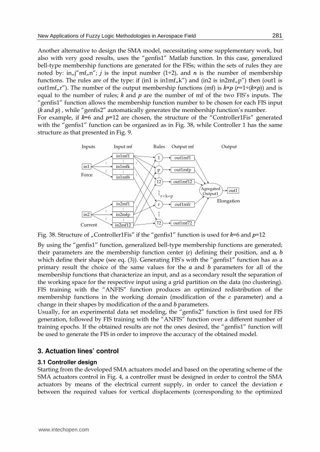
Another alternative to design the SMA model, necessitating some supplementary work, but also with very good results, uses the “genfis1” Matlab function. In this case, generalized bell-type membership functions are generated for the FISs; within the sets of rules they are noted by: in„j”mf„n”; j is the input number (1÷2), and n is the number of membership functions. The rules are of the type: if (in1 is in1mf„k”) and (in2 is in2mf„p”) then (out1 is out1mf„r”). The number of the output membership functions (mf) is k×p (r=1÷(k×p)) and is equal to the number of rules; k and p are the number of mf of the two FIS’s inputs. The “genfis1” function allows the membership function number to be chosen for each FIS input (k and p) , while “genfis2” automatically generates the membership function’s number. For example, if k=6 and p=12 are chosen, the structure of the “Controller1Fis” generated with the “genfis1” function can be organized as in Fig. 38, while Controller 1 has the same structure as that presented in Fig. 9.
out1
in1
in1mf1
in1mfk
in1mf6
......
Inputs Input mf Rules Output mf
......
1
out1mfp
in2
in2mf1
in2mfp
in2mf12
......
......
...
......
......
out1mfr
out1mf72
AgregatedOutput1
Output
Force
Current
Elongation
p
72
12
r
pkr ×=
out1mf12
out1mf1...
......
Fig. 38. Structure of „Controller1Fis” if the “genfis1” function is used for k=6 and p=12
By using the “genfis1” function, generalized bell-type membership functions are generated; their parameters are the membership function center (c) defining their position, and a, b which define their shape (see eq. (3)). Generating FIS’s with the “genfis1” function has as a primary result the choice of the same values for the a and b parameters for all of the membership functions that characterize an input, and as a secondary result the separation of the working space for the respective input using a grid partition on the data (no clustering). FIS training with the “ANFIS” function produces an optimized redistribution of the membership functions in the working domain (modification of the c parameter) and a change in their shapes by modification of the a and b parameters. Usually, for an experimental data set modeling, the “genfis2” function is first used for FIS generation, followed by FIS training with the “ANFIS” function over a different number of training epochs. If the obtained results are not the ones desired, the “genfis1” function will be used to generate the FIS in order to improve the accuracy of the obtained model.
3. Actuation lines’ control
3.1 Controller design Starting from the developed SMA actuators model and based on the operating scheme of the SMA actuators control in Fig. 4, a controller must be designed in order to control the SMA actuators by means of the electrical current supply, in order to cancel the deviation e between the required values for vertical displacements (corresponding to the optimized
www.intechopen.com

Fuzzy Controllers, Theory and Applications
282
airfoils) and the real values, obtained from two position transducers. The design of such a controller is difficult due to the strong nonlinearities of the SMA actuators’ characteristics. In these conditions, and considering our research team experience in fuzzy logic control systems design, we decided that one variant of control would be developed with fuzzy logic. The simplest fuzzy logic controller is the Fuzzy Proportional (FP) controller, being relevant for state or output feedback in a state space controller. Its input is the error and the output is the control signal. From another perspective, derivative action helps to predict the error, and the Proportional-Derivative (PD) controller uses further the derivative action to improve closed-loop stability (Jantzen, 1998). The equation of a PD controller can be expressed as follows:
,d
)(d)(
d
)(d)()( ⎥⎦
⎤⎢⎣⎡ ⋅+⋅=⋅+⋅=
tte
TteKtte
KteKti DPDP (15)
where i(t) is the command variable (electrical current in our case), that is time dependent; e is the operating error (see Fig. 4), KP is the proportional gain and KD is the derivative gain. In discrete form, the equation (15) becomes (Kumar et al., 2008):
),()()( keKkeKki DP Δ⋅+⋅= (16)
,)]1()([
)()(S
DP Tkeke
KkeKki−−⋅+⋅= (17)
where k is the discrete step, ST is the sample period, and )(keΔ is the change in error.
Therefore, the inputs to the Fuzzy Proportional-Derivative (FPD) controller are the error and
its derivative (called change in error in fuzzy control language), while the output is the
control signal. We have chosen the structure shown in Fig. 39 for our FLC, where KD is the
change in the output gain.
i
Command
Fuzzy
rule base
KP
Proportionalgain
e
KD
Δe
Derivativegain
KO
Change inoutput gain
Error
Changein error
FPD controller
Fig. 39. Fuzzy PD controller architecture
To realize the input-output mapping of the designed controller, we must consider that in the SMA cooling phase the actuators would not be powered or the supplying current would be very small. This cooling phase may occur not only when controlling a long-term phase, when a switch between two values of the actuator displacements is ordered, but also in a short-lived phase, which occurs when the real value of the deformation exceeds its desired value and the actuator wires need to be cooled. Each of the FLC input or output signals have the real line as the universe of discourse. In practice, the universe of discourse is restricted to a comparatively small interval, many
www.intechopen.com

New Applications of Fuzzy Logic Methodologies in Aerospace Field
283
authors and several commercial controllers using standard universes such as [-1, 1], or [-100, 100] corresponding to percentages of full scale. For our system, the [-1, 1] interval was chosen as the universe for inputs signals, and [0, 2.5] interval was chosen as the universe for output signal. Also, following numerical simulations, we have chosen a number of three membership functions for each of the two inputs, and three membership functions for the output. The shapes chosen for inputs membership functions were s-functions, ┨-functions, and z-functions. Generally, an s-function shaped membership function can be implemented using a cosine function:
,
if,1
if,cos12
1
if,0
),,(
⎪⎪⎩
⎪⎪⎨⎧
>≤≤⎥⎥⎦
⎤⎢⎢⎣⎡
⎟⎟⎠⎞
⎜⎜⎝⎛ π−
−+<
=right
rightleft
leftright
right
left
rightleft
xx
xxxxx
xx
xx
xxxs (18)
a z-function shaped membership function is a reflection of a shaped s-function:
,
if,0
if,cos12
1
if,1
),,(
⎪⎪⎩
⎪⎪⎨⎧
>≤≤⎥⎥⎦
⎤⎢⎢⎣⎡
⎟⎟⎠⎞
⎜⎜⎝⎛ π−
−+<
=right
rightleft
leftright
left
left
rightleft
xx
xxxxx
xx
xx
xxxz (19)
and a ┨ -function shaped membership function is a combination of both functions:
)],,,(),,,(min[),,,,(21121
xxxzxxxsxxxxx rightmmleftrightmmleft =π (20)
with the peak flat over the [xm1, xm2] middle interval. x is the independent variable on the
universe, xleft is the left breakpoint, and xright is the right breakpoint (Jantzen, 1998).
To define the rules, a Sugeno fuzzy model was chosen, which for a two input - single output
system with N rules is given by eq. (5):
.),(then,isandisIf:Rule
,),(then,isandisIf:Rule
,),(then,isandisIf:1Rule
22110212211
22110212211
2
1
21
1
1
1
021
11
22
1
11
xaxabxxyAxAxN
xaxabxxyAxAxi
xaxabxxyAxAx
NNNNNN
iiiiii
++=++=++=
B
B (21)
In the [-1, 1] universe interval, a three range partition, Negative (N), Zero (Z) and Positive
(P), were chosen for the inputs e and Δe while in the [0, 2.5] universe interval three-range
partition, Zero (Z), Positive-Small (PS) and Positive-Big (PB) were used for the output.
According to the values in the Table 5, the membership functions for the inputs are by the
form depicted in Fig. 40, and are given by the eq. (18), (19) or (20):
[ ] ,
0if,0
05.0if,)12cos(12
15.0if,1
),0,5.0()(1
1
⎪⎪⎩⎪⎪⎨⎧
>≤≤−π++
−<=−=
x
xx
x
xzxA (22)
www.intechopen.com

Fuzzy Controllers, Theory and Applications
284
[ ] ,
0if,0
01if,)1cos(12
11if,1
),0,1()(1
2
⎪⎪⎩⎪⎪⎨⎧
>≤≤−π++
−<=−=
x
xx
x
xzxA (23)
[ ] ,
1if,0
11if,)cos(12
11if,0
)],1,0(),,0,1(min[),1,0,0,1()(2
1
⎪⎪⎩⎪⎪⎨⎧
>≤≤−π+
−<=−=−π=
x
xx
x
xzxsxxA (24)
,
1if,0
11.0if,9
110cos1
2
1
1.01.0if,1
1.01if,9
110cos1
2
1
1if,0
),1,1.0,1.0,1()(2
2
⎪⎪⎪⎪
⎩
⎪⎪⎪⎪
⎨
⎧
>≤≤⎥⎦
⎤⎢⎣⎡ π⎟⎠
⎞⎜⎝⎛ −+
<<−−≤≤−⎥⎦
⎤⎢⎣⎡ π⎟⎠
⎞⎜⎝⎛ ++
−<
=−−π=
x
xx
x
xx
x
xxA (25)
[ ] .
1if,1
10if,)1cos(12
10if,0
),1,0()()( 3
2
3
1
⎪⎪⎩⎪⎪⎨⎧
>≤≤π−+
<===
x
xx
x
xsxAxA (26)
mf parameters Input mf mf type
xleft xm1 xm2 xright mf1 )( 1
1A z - function -0.5 - - 0
mf2 )( 2
1A ┨ -function -1 0 0 1 e
mf3 )( 3
1A s - function 0 - - 1
mf1 )( 1
2A z - function -1 - - 0
mf2 )( 2
2A ┨ - function -1 -0.1 -0.1 1 eΔ
mf3 )( 3
2A s - function 0 - - 1
Table 5. Parameters of the input’s membership functions
For the output membership functions constant values were chosen (Z=0, PS=1.25, PB=2.5),
so the values of ),1,2,1( Nikai
k == parameters in eq. (21) were zero. Starting from the
inputs’ and output’s membership functions, a set of 5 inference rules were obtained (N=5):
.0),(then,isandisIf:5Rule
,0),(then,isandisIf:4Rule
,5.1),(then,isandisIf:3Rule
,0),(then,isandisIf:2Rule
,5.2),(then,isandisIf:1Rule
52
2
3
1
43
2
2
1
31
2
2
1
23
2
1
1
12
2
1
1
=ΔΔ=ΔΔ=ΔΔ=ΔΔ=ΔΔ
eeyAeAe
eeyAeAe
eeyAeAe
eeyAeAe
eeyAeAe
(27)
www.intechopen.com

New Applications of Fuzzy Logic Methodologies in Aerospace Field
285
input 2 (Δe)
Deg
ree
of
mem
ber
ship
0
0.2
0.4
0.6
0.8
1
mf1 (N) mf2 (Z) mf3 (P)
-1 -0.8 -0.6 -0.4 -0.2 0 0.2 0.4 0.6 0.8 1
input 1 (e)D
egre
e o
f m
emb
ersh
ip
0
0.2
0.4
0.6
0.8
1
mf1 (N) mf2 (Z) mf3 (P)
-1 -0.8 -0.6 -0.4 -0.2 0 0.2 0.4 0.6 0.8 1
Fig. 40. Membership functions for the fuzzy logic controller inputs
The rule-based inference chosen for each consequent is presented in Table 6. With the
previous considerations, the fuzzy control surface results by the form presented in Fig. 41
(two views for different angles).
Δe/e N Z P
N - PS(1.25) -
Z PB(2.5) - Z(0)
P Z(0) Z(0) -
Table 6. Rule-based inference for the fuzzy logic controller
-1
-0.5
0
0.5
1 -1
-0.5
0
0.5
1
input 2 (Δe)input 1 (e)
ou
tpu
t
00.5
11.5
22.5
-1
-0.5
0
0.5
1
-1-0.5
00.5
1input 2 (Δe)
input 1 (e)
ou
tpu
t
00.5
11.5
22.5
Fig. 41. The fuzzy control surface (two views for different angles)
3.2 Actuation lines’ controller implementation and numerical simulation Implementing the operating scheme of the SMA actuators control (Fig. 4) in Matlab-
Simulink, the model shown in Fig. 42 was obtained. The input variable of the scheme is the
desired skin deflection, while the output is the real skin deflection.
www.intechopen.com

Fuzzy Controllers, Theory and Applications
286
0
SMA elongation [m]skin deflection [mm]
skin
deflection
[mm]
desired deflection[mm]
SMAelongation
[m]
0
skin deflexion [mm]
1
1 6
desired
deflection
[mm]
3
cam factor
ScopeCurrent
ForceDisplacement
SMA Fuzzy Model
1.8
SMA Initial length
Memory1
F aero [N]
x [m]
F SMA [N]
y [mm]
Mechanical system
Diff errorCurrent
out
FPD controller
0
Current [A]
1150
Aerodynamic
force [N]
Fig. 42. The simulation model for the controlled SMA actuator with the neuro-fuzzy model
The “FPD controller” block contains the implementation of the controller presented in Fig. 39; the detailed Simulink scheme of this block is shown in Fig. 43. The block has as input the control error (the difference between the desired and the obtained displacements), and the controlled electrical current applied on the SMA actuators as output. The “SMA Fuzzy Model” block has the schema presented in Fig. 34; its inputs are the SMA loading force and the electrical current, while its output is the SMA elongation. The “Mechanical System” block in Fig. 43 models the SMA loading force starting from the aerodynamic force, skin elastic force, gas spring elastic force and gas spring pretension force.
Current out
1
Gain 1
-K-
Gain
-K-
Gain 2
-K-
Fuzzy Logic
ControllerDerivative
2z-2
den (z)Diff error
1
Fig. 43. “FPD controller” block in Simulink
To obtain an automatic control system, the preloaded forces on the gas springs in the two actuation lines must be valid for all 35 studied cases. By estimating the aerodynamic forces for all 35 studied flight conditions and optimized airfoils, a compromise should be done to balance the aerodynamic forces with the preloaded forces of the gas spring. Following estimation calculations, the pretension force of the gas springs in “Mechanical system” Simulink block (see Fig. 42) was considered with the value of 1250 N. In this situation, if the simulated model in Fig. 42 was loaded with an aerodynamic force Faero=1150 N, for a successive steps input signal applied to the controlled actuator, the characteristics shown in Fig. 44 are obtained. The results shown in Fig. 44 confirm that the obtained FPD controller works very well in both phases (heating and cooling) of the SMA actuators. To see the manner in which the controller works, screenshots were taken at different times of the numerical simulation presented in Fig. 44. The screenshots (Fig. 45) highlighted the fuzzy model input-output mapping of the eight analyzed points (P1÷P8). The chosen time values, shown on Fig. 44, are: 11.67 s (P1), 27.03 s (P2), 29.40 s (P3), 55.32 s (P4), 62.75 s (P5), 108.42 s (P6), 119.12 s (P7)
www.intechopen.com

New Applications of Fuzzy Logic Methodologies in Aerospace Field
287
P1
P2
P3
P4 P5
P6P7
P8S
kin
def
lect
ion
[m
m]
-1
0
1
2
3
4
5
6
7
8
Time [s]0 20 40 60 80 100 120 140 160
obtaineddesiredanalyzed points
Fig. 44. Response for a successive steps input when Faero=1150 N and Fpretension=1250 N
127.71 s (P8). Fig. 45 shows that the correspondence between the membership functions of
the inputs and the membership functions of the output through the inference engine of the
designed fuzzy model was correctly established. The same observation can be found by
correlating Fig. 45 with the positions of the analyzed points in Fig. 44 and with the error e
and change in error Δe signs and trends.
3.3 Bench test and wind tunnel experimental validation From the SMA theory and based on the numerical simulations of the morphing wing
system, the limits for the electrical current used to drive the actuators, correlated with the
SMA temperature and SMA loading force, were estimated. As a consequence, two
Programmable Switching Power Supplies AMREL SPS100-33 (Brailovski et al., 2008; Coutu
et al., 2007; Coutu et al., 2009), controlled by Matlab/Simulink through a Quanser Q8 data
acquisition card (Fig. 46) were chosen to implement the controller model (Austerlitz, 2002;
Kirianaki et al., 2002; Park & Mackay, 2003). The AMREL SPS100-33 Power Supplies have
RS-232 and GPIB IEEE-488 as standard features, and their technical characteristics include:
Power 3.3kW, Voltage (dc) 0-100 V, Current (dc) 0-33 A. The Quanser data acquisition card
has 8 single-ended analog inputs with 14-bit resolution, which can be sampled
simultaneously at 100 kHz, with A/D conversion times of 2.4 µs/channel, and is equipped
with 8 analog outputs, software programmable voltage ranges, that allow the control of the
SMA actuators.
The Q8 data acquisition card was connected to a PC and programmed via Matlab/Simulink
R2006b and WinCon 5.2 (Fig. 47).
As observed on Fig. 47, all data acquisition card single-ended analog inputs were used: two
signals indicating the vertical displacements dY1 and dY2 of the SMA actuators are provided
by two Linear Variable Differential Transformer (LVDT) potentiometers, and six signals are
provided by six thermocouples installed on each of the SMA wires’ components. Two of the
card output channels were used to control each power supply through analog/external
control by means of a DB-15 I/O connector, and other two card output channels were used
to start the power supplies with a 5V analog signal. The “SMA1” block had the scheme
presented in Fig. 48.
www.intechopen.com

Fuzzy Controllers, Theory and Applications
288
Fig. 45. Fuzzy model input-output mapping of the analyzed points
As seen in Fig. 48, the “SMA1” block, controlling the first actuation line, contains the
implementation of the controller presented in Fig. 43 and the observations related to the
SMA actuators’ physical limitations in terms of temperature and supplying currents. The
current supplied to the actuator was limited at 10A, and the control signal was set to be 0-
0.606V (maximum voltage for the power supply is 2V for a 33A current supply). The upper
limit of the SMA wires temperature in the “Temperature limiter” block was established at
P1 (11.67 s) P2 (27.03 s)
P3 (29.40 s) P4 (55.32 s)
P5 (62.75 s) P6 (108.42 s)
P7 (119.12 s) P8 (127.71 s)
www.intechopen.com

New Applications of Fuzzy Logic Methodologies in Aerospace Field
289
130˚C. The control scheme in Fig. 43 was improved with conditioners related to physical
model protection. In this way, a software protection of the actuation lines was realized.
dY1
dY2
SMA#1 SMA#2
... pressure sensors
Optimumairfoil
Reference airfoil
Output signal forpower supply control
AMREL SPS100-33power supplies
Positiontransducers
Quanser Q8 dataacquisition card
Signal from positiontransducers Real
dY1, dY
2
...
Signal from sixthermocouples
Morphing wing
DesireddY
1, dY
2
Fig. 46. Bench test physical model operating schema
0
Volts
Temp
StartVolt
termocouple1
termocouple2
termocouple3
position 2
temp
amps
control V
start 5V
SMA2
termocouple1
termocouple2
termocouple3
position 1
temp
amps
control V
start 5V
SMA1
Q8
Quanser
Analog Input
Amps
Analog Input
0
Q8
Quanser
Analog Output
Analog Output
Fig. 47. Q8 data acquisition card using to control the actuators
After some tests with the experimental model, the preloaded force of the gas springs that
maintains the SMA wires in tension was chosen to be 1000 N, since in the laboratory the
existence of aerodynamic forces could not be considered.
The Matlab/Simulink implemented controller was used in the same way for both actuation
lines of the morphing wing system, so the “SMA2” block had a similar scheme to the
“SMA1” block, with the exception of the numerical values of the thermocouples calibration
gains and constants.
www.intechopen.com
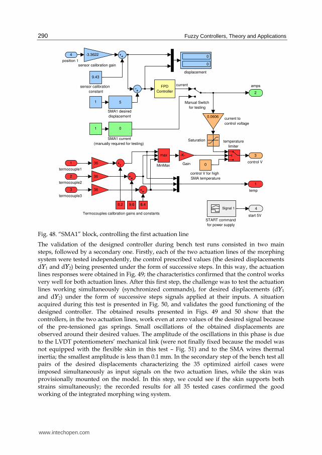
Fuzzy Controllers, Theory and Applications
290
Termocouples calibration gains and constants
4
start 5V
3
control V
2
amps
1
temp
temperature
limiter
-3.3622
sensor calibration gain
9.43
sensor calibration
constant
0
displacement
0.0606current to
control voltage
0
control V for high
SMA temperature
36
36
36
Saturation
Signal 1
START command
for power supply
5
SMA1 desired
displacement
0
SMA1 current
(manually required for testing)
max
MinMax
Manual Switch
for testing
-K-
Gain
1
8.49.6
1
8.2
4
position 1
3
termocouple3
2
termocouple2
1
termocouple1
0
currentFPD
Controller
Fig. 48. “SMA1” block, controlling the first actuation line
The validation of the designed controller during bench test runs consisted in two main steps, followed by a secondary one. Firstly, each of the two actuation lines of the morphing system were tested independently, the control prescribed values (the desired displacements dY1 and dY2) being presented under the form of successive steps. In this way, the actuation lines responses were obtained in Fig. 49; the characteristics confirmed that the control works very well for both actuation lines. After this first step, the challenge was to test the actuation lines working simultaneously (synchronized commands), for desired displacements (dY1 and dY2) under the form of successive steps signals applied at their inputs. A situation acquired during this test is presented in Fig. 50, and validates the good functioning of the designed controller. The obtained results presented in Figs. 49 and 50 show that the controllers, in the two actuation lines, work even at zero values of the desired signal because of the pre-tensioned gas springs. Small oscillations of the obtained displacements are observed around their desired values. The amplitude of the oscillations in this phase is due to the LVDT potentiometers’ mechanical link (were not finally fixed because the model was not equipped with the flexible skin in this test – Fig. 51) and to the SMA wires thermal inertia; the smallest amplitude is less than 0.1 mm. In the secondary step of the bench test all pairs of the desired displacements characterizing the 35 optimized airfoil cases were imposed simultaneously as input signals on the two actuation lines, while the skin was provisionally mounted on the model. In this step, we could see if the skin supports both strains simultaneously; the recorded results for all 35 tested cases confirmed the good working of the integrated morphing wing system.
www.intechopen.com

New Applications of Fuzzy Logic Methodologies in Aerospace Field
291
-1
0
1
2
3
4
5
6
Time [s]
Dis
pla
cem
ent
dY
1 [m
m]
act #1 desired
act #1 obtained
0 100 200 300 400 500 600 700 800 900 1000Time [s]
0 100 200 300 400 500 600 700 800 900 1000-1
0
1
2
3
4
5
6
7
8
Dis
pla
cem
ent
dY
2 [m
m]
act #2 desired
act #2 obtained
Fig. 49. Actuation lines independent bench test
This secondary step of the bench test was considered in wind tunnel, and get together with the transition point real time position detection and visualization, in order to validate experimentally all of the 35 optimized airfoils theoretically obtained. A typical test for one of the 35 flight conditions consisted in a wind tunnel tare run, followed by a run for the reference (un-morphed) airfoil, and finally by a run for morphed airfoil, reproducing the corresponding optimized airfoil. The morphing wing system during wind tunnel tests is shown in Fig. 52.
act #1 desired
act #1 obtained
-1
0
1
2
3
4
5
6
7
Dis
pla
cem
ent
dY
1 [m
m]
0 100 200 300 400 500 600 700 800 900Time [s]
-1
0
1
2
3
4
5
6
7
8
0 100 200 300 400 500 600 700 800 900
Dis
pla
cem
ent
dY
2 [m
m]
Time [s]
act #2 desired
act #2 obtained
Fig. 50. Actuation lines simultaneously bench test
Fig. 51. Morphing wing system in the bench test
www.intechopen.com

Fuzzy Controllers, Theory and Applications
292
Fig. 52. Morphing wing system in the wind tunnel test runs
Because of the presence of the aerodynamic forces on the flexible skin of the wing for the wind tunnel tests, the preloaded forces of the gas springs were reconsidered at 1500 N. The control results for test run 42, characterized by the angle of attack α=2° and Mach number Mach=0.2 (deflections of both actuators are dY1=5.73 mm and dY2=7.45 mm), are shown in Fig 53.
-1
0
1
2
3
4
5
6
dY1=5.73 mm
Dis
pla
cem
ent
dY
1 [
mm
]
act #1 desired
act #1 obtained
Time [s]0 20 40 60 80 100 120 140 160 180 200
Time [s]0 20 40 60 80 100 120 140 160 180 200
act #2 desired
act #2 obtaineddY2=7.45 mm
-1
0
1
2
3
4
5
6
7
8
Dis
pla
cem
ent
dY
2 [m
m]
20 30 40 50 60 70 80-1
0
1
2
3
4
5
6
7
8
Dis
pla
cem
ents
dY
1, d
Y2
[mm
]
Temperature [oC]
act #1act #2
Time [s]0 20 40 60 80 100 120 140 160 180 200
20
30
40
50
60
70
80
Tem
per
atu
re [
oC
]
act #1act #2
Fig. 53. Wind Tunnel Test for α=2°, Mach=0.2 (dY1=5.73 mm, dY2=7.45 mm)
From the experimental results, it can still be observed a high frequency noise influencing the LVDT sensors and thermocouple’s instrumentation amplifiers, but with small amplitudes with respect to those for the bench tested cases. A positive impact on the noise amplitude
www.intechopen.com

New Applications of Fuzzy Logic Methodologies in Aerospace Field
293
reduction is the completion of mechanical model by final fixing of the skin on the model; this time, the noise sources are the wind tunnel vibrations, the instrumentation electrical fields and the wind tunnel supplying and monitoring equipments electrical fields. Fig. 53 and all the tested situations results confirmed that the designed controller works very well in the wind tunnel, being positively influenced by the aerodynamic forces presence.
4. Conclusions
The approaches for the design and to the validation of a morphing wing fuzzy logic application were presented. The developed morphing mechanism used smart materials such as Shape Memory Alloy (SMA) in the actuation control concept. Two important applications of the fuzzy logic technique were highlighted in this work: the identification of a model for a system starting from some experimental input-output data, and the automatic control of a system. In this way, in our morphing application two directions were developed: smart material actuator modeling and actuation lines’ control. Based on a neuro-fuzzy network and using numerical values resulted from the SMA experimental testing (forces, currents, temperatures and elongations), an empirical model was developed for the SMA actuators that could be used in the design phase of the actuation lines’ control. The SMA testing was performed at Tamb=24˚C for six load cases with the forces of 700 N, 850 N, 1000 N, 1100 N, 1250 N and 1500 N. The electrical currents following the increasing-constant-decreasing-zero values evolution were applied on the SMA actuator in each of the six cases considered. Four Fuzzy Inference Systems (FIS’s) were used to obtain four neuro-fuzzy controllers: one controller for the current increase, one for a constant current, one for the current decrease, and one controller for the null current (after its decrease). For the first and for the third controllers, inputs such as the force and the current were used, while for the second and the fourth controllers, inputs such as the force and the time values reflecting the SMA thermal inertia were used. Finally, the four obtained controllers were integrated into a single controller. The “genfis2” Matlab function was used to generate and train the fuzzy inference systems associated with the four controllers. The four initially obtained fuzzy inference systems were trained for 5000, 100000, 20000, and 250000 training epochs. For the four FISs, the mean of the relative absolute values of the errors decreased from 0.3063%, 3.3503%, 1.5154·10-3 %, and 5.1855%, respectively, before training, to 0.119%, 0.8902%, 2.3106·10-13 %, and 1.0316%, respectively, after training. Evaluating the model obtained for the SMA actuators (the final, integrated controller) in all six cases of experimental data, the mean values of the relative absolute errors were: 1.7538% for 700N, 1.2738% for 850N, 1.0964% for 1000N, 0.5228% for 1100N, 0.7179% for 1250N, and 0.2532 for 1250N. Therefore, the mean value of the relative absolute error between the experimental data and the outputs of the obtained model was 0.9363%. A very important advantage of this new model is its rapid generation, since the “genfis2” and “ANFIS” functions are already implemented in Matlab. The user only needs to assume the four FIS’s training performances using the “anfisedit” interface generated with Matlab. The second application of fuzzy-logic techniques in our project (actuation lines’ control) supposed the design of an SMA actuators’ controller starting from the developed SMA actuators’ model. The controller was designed to control the SMA actuators by means of the electrical current supply, in order to cancel the deviation e between the required values for
www.intechopen.com

Fuzzy Controllers, Theory and Applications
294
vertical displacements (corresponding to the optimized airfoils) and the real values, obtained from two position transducers. Finally, a fuzzy PD architecture was chosen for the controller. In its design, numerical simulations of the open loop morphing wing integrated system, based on a SMA neuro-fuzzy model, were performed. A bench test and a wind tunnel test were conducted as subsequent validation methods. A [-1, 1] interval was chosen as the universe for the inputs’ signals, and a [0, 2.5] interval was chosen as the universe for the output signal. Also, following numerical simulations, three membership functions for each of the two inputs, and three membership functions for the output were chosen. The experimental validation tests (bench tests and wind tunnel test) confirmed that the designed controller works very well. The wind tunnel tests were quite positive, with their transition point real time position detection and visualization, which experimentally validated all of the 35 theoretically-obtained optimized airfoils. As a general conclusion, the work presented here has proved the feasibility of using fuzzy logic methodologies in multidisciplinary research studies in the aerospace field, especially for morphing wing or morphing aircraft studies.
5. References
Al-Odienat, A.I. & Al-Lawama, A.A. (2008). The Advantages of PID Fuzzy Controllers Over The Conventional Types, American Journal of Applied Sciences, Vol. 5, No. 6, pp. 653-658, June 2008, ISSN: 1546-9239
Austerlitz, H. (2002). Data acquisition techniques using PCs, Elsevier, ISBN: 978-0-12-068377-2, USA
Baron, A.; Benedict, B.; Branchaw, N.; Ostry, B.; Pearsall, J.; Perlman, G. & Selstrom, J. (2003). Morphing Wing (MoW), ASEN 4018 Senior Projects Technical Report, Department of Aerospace Engineering, University of Colorado, December 2003, Boulder, Colorado, USA, 102 pages
Brailovski, V.; Terriault, P.; Coutu, D.; Georges, T.; Morellon, E.; Fischer, C. & Berube, S. (2008). Morphing laminar wing with flexible extrados powered by shape memory alloy actuators, Proceedings of ASME 2008 Conference on Smart Materials, Adaptive Structures and Intelligent Systems (SMASIS2008), pp. 615-623, ISBN: 978-0-7918-4331-4, Maryland, USA, October 28–30, 2008, Publisher ASME, Ellicott City
Coutu, D.; Brailovski, V.; Terriault, P. & Fischer, C. (2007). Experimental validation of the 3D numerical model for an adaptive laminar wing with flexible extrados, Proceedings of the 18th International Conference of Adaptive Structures and Technologies, 10 pages, Ottawa, Ontario, Canada, 3-5 October, 2007
Coutu, D.; Brailovski, V. & Terriault, P. (2009). Promising benefits of an active-extrados morphing laminar wing, AIAA Journal of Aircraft, Vol. 46, No. 2, pp. 730-731, March-April 2009, ISSN: 0021-8669
Georges, T.; Brailovski, V.; Morellon, E.; Coutu, D. & Terriault, P. (2009). Design of Shape Memory Alloy Actuators for Morphing Laminar Wing With Flexible Extrados, Journal of Mechanical Design, Vol. 131, No. 9, 9 pages, 091006, September 2009, ISSN: 1050-0472
Gonzalez, L. (2005). Morphing Wing Using Shape Memory Alloy: A Concept Proposal, Final research paper in 2005 Summer Research Experience for Undergraduates (REU) on Nanotechnology and Materials Systems, Texas Institute of Intelligent Bio-Nano
www.intechopen.com

New Applications of Fuzzy Logic Methodologies in Aerospace Field
295
Materials and Structures for Aerospace Vehicles (TiiMS) – NASA Research University, Texas A&M University, July 2005, College Station, Texas, USA
Grigorie, T.L. & Botez, R.M. (2009). Adaptive neuro-fuzzy inference system based controllers for Smart Material Actuator modeling, Proceedings of the Institution of Mechanical Engineers, Part G: Journal of Aerospace Engineering, Vol. 223, No. 6, pp. 655-668, June 2009, ISSN: 0954-4100
Grigorie, T.L. & Botez, R.M. (2010). New adaptive controller method for SMA hysteresis modeling of a morphing wing, The Aeronautical Journal, Vol. 114, No. 1151, pp. 1-13, January 2010, ISSN: 0001-9240
Grigorie, T.L.; Popov, A.V.; Botez, R.M.; Mébarki, Y. & Mamou, M. (2010 a). Modeling and testing of a morphing wing in open-loop architecture, AIAA Journal of Aircraft, Vol. 47, No. 3, pp. 917-923, May–June 2010, ISSN: 0021-8669
Grigorie, T. L.; Popov, A.V.; Botez, R.M.; Mamou, M. & Mebarki, Y. (2010 b). A morphing wing used shape memory alloy actuators new control technique with bi-positional and PI laws optimum combination. Part 1: design phase, Proceedings of the 7th International Conference on Informatics in Control, Automation and Robotics ICINCO 2010, pp. 5-12, ISBN: 978-989-8425-00-3, Madeira, Portugal, 15-18 June, 2010, SciTePress – Science and Technology Publications, Funchal
Grigorie, T. L.; Popov, A.V.; Botez, R.M.; Mamou, M. & Mebarki, Y. (2010 c). A morphing wing used shape memory alloy actuators new control technique with bi-positional and PI laws optimum combination. Part 2: experimental validation, Proceedings of the 7th International Conference on Informatics in Control, Automation and Robotics ICINCO 2010, pp. 13-19, ISBN: 978-989-8425-00-3, Madeira, Portugal, 15-18 June, 2010, SciTePress – Science and Technology Publications, Funchal
Hampel, R.; Wagenknecht, M. & Chaker, N. (2000). Fuzzy Control – Theory and Practice, Physica-Verlag, ISBN-13: 978-3790813272, USA
Jantzen, J. (1998). Tuning of fuzzy PID controllers, Technical Report 98-H871, Department of Automation, Technical University of Denmark, September 1998, 22 pages
Khezri, M. & Jahed, M. (2007). Real-time intelligent pattern recognition algorithm for surface EMG signals, BioMedical Engineering OnLine, Vol. 6, Paper 45, 12 pages, December 2007, ISSN: 1475-925X
Kirianaki, N.V.; Yurish, S.Y; Shpak, N.O. & Deynega, V.P. (2002). Data Acquisition and Signal Processing for Smart Sensors. John Wiley & Sons, ISBN: 978-0470843178, UK
Kosko, B. (1992). Neural networks and fuzzy systems – A dynamical systems approach to machine intelligence, Prentice Hall, ISBN: 978-0136114352, New Jersey, USA
Kovacic, Z. & Bogdan, S. (2006). Fuzzy Controller Design – Theory and applications, Taylor and Francis Group, ISBN: 978-0849337475, USA
Kumar, V.; Rana, K.P.S. & Gupta, V. (2008). Real-Time Performance Evaluation of a Fuzzy PI + Fuzzy PD Controller for Liquid-Level Process, International Journal of Intelligent Control and Systems, Vol. 13, No. 2, pp. 89-96, June 2008, ISSN: 0218-7965
Kung, C.C. & Su, J.Y. (2007). Affine Takagi-Sugeno fuzzy modelling algorithm by fuzzy c-regression models clustering with a novel cluster validity criterion, IET Control Theory and Applications, Vol. 1, No. 5, pp. 1255-1265, September 2007, ISSN: 1751-8644
Mahfouf, M.; Linkens, D.A. & Kandiah, S. (1999). Fuzzy Takagi-Sugeno Kang model predictive control for process engineering, IEE Workshop on Model Predictive Control:
www.intechopen.com

Fuzzy Controllers, Theory and Applications
296
Techniques and Applications, 4 pages, 29 April, 1999, Printed and published by the IEE, Savoy place, London WCPR OBL, UK
MathWorks Inc. (2008), Matlab Fuzzy Logic and Neural Network Toolboxes - Help. Park, J. & Mackay, S. (2003). Practical data acquisition for instrumentation and control systems,
Elsevier, ISBN: 978-0750657969, UK Popov, A.V.; Botez, R.M. & Labib, M. (2008 a). Transition point detection from the surface
pressure distribution for controller design, AIAA Journal of Aircraft, Vol. 45, No. 1, pp. 23-28, January-February 2008, ISSN: 0021-8669
Popov, A.V.; Labib, M.; Fays, J. & Botez, R.M. (2008 b). Closed loop control simulations on a morphing laminar airfoil using shape memory alloys actuators, AIAA Journal of Aircraft, Vol. 45, No. 5, pp. 1794-1803, September-October 2008, ISSN: 0021-8669
Popov, A.V.; Botez, R.M.; Mamou, M.; Mebarki, Y.; Jahrhaus, B.; Khalid. M. & Grigorie, T.L. (2009 a). Drag reduction by improving laminar flows past morphing configurations, AVT-168 NATO Symposium on the Morphing Vehicles, 12 pages, 20-23 April, 2009, Published by NATO, Evora, Portugal
Popov, A.V.; Botez, R. M.; Mamou, M. & Grigorie, T.L. (2009 b). Optical sensor pressure measurements variations with temperature in wind tunnel testing, AIAA Journal of Aircraft, Vol. 46, No. 4, pp. 1314-1318, July-August 2009, ISSN: 0021-8669
Popov, A.V.; Grigorie, T. L.; Botez, R.M.; Mamou, M. & Mebarki, Y. (2010 a). Morphing wing real time optimization in wind tunnel tests, Proceedings of the 7th International Conference on Informatics in Control, Automation and Robotics ICINCO 2010, pp. 114-124, ISBN: 978-989-8425-00-3, Madeira, Portugal, 15-18 June, 2010, SciTePress – Science and Technology Publications, Funchal
Popov, A.V.; Grigorie, T. L.; Botez, R.M.; Mamou, M. & Mebarki, Y. (2010 b). Closed-Loop Control Validation of a Morphing Wing Using Wind Tunnel Tests, AIAA Journal of Aircraft, Vol. 47, No. 4, pp. 1309-1317, July–August 2010, ISSN: 0021-8669
Popov, A.V.; Grigorie, T. L.; Botez, R.M.; Mamou, M. & Mebarki, Y. (2010 c). Real Time Morphing Wing Optimization Validation Using Wind-Tunnel Tests, AIAA Journal of Aircraft, Vol. 47, No. 4, pp. 1346-1355, July–August 2010, ISSN: 0021-8669
Sainmont, C.; Paraschivoiu, I. & Coutu, D. (2009). Multidisciplinary Approach for the Optimization of a Laminar Airfoil Equipped with a Morphing Upper Surface, AVT-168 NATO Symposium on the Morphing Vehicles, 20-23 April, 2009, Published by NATO, Evora, Portugal
Sivanandam, S.N.; Sumathi, S. & Deepa, S.N. (2007). Introduction to Fuzzy Logic using MATLAB, Springer, ISBN: 978-3540357803, Berlin, Heidelberg, New York
Thill, C.; Etches, J.; Bond, I.; Potter, K. & Weaver, P. (2008). Morphing skins, The Aeronautical Journal, Vol. 112, No. 1129, pp. 117-139, March 2008, ISSN: 0001-9240
Verbruggen, H.B. & Bruijn, P.M. (1997). Fuzzy control and conventional control: What is (and can be) the real contribution of Fuzzy Systems?, Fuzzy Sets Systems, Vol. 90, No. 2, pp. 151–160, September 1997, ISSN: 0165-0114
Zadeh, L.A. (1965). Fuzzy sets, Information and Control, Vol. 8, No. 3, pp. 339-353, June 1965, ISSN: 00199958
www.intechopen.com

Fuzzy Controllers, Theory and ApplicationsEdited by Dr. Lucian Grigorie
ISBN 978-953-307-543-3Hard cover, 368 pagesPublisher InTechPublished online 28, February, 2011Published in print edition February, 2011
InTech EuropeUniversity Campus STeP Ri Slavka Krautzeka 83/A 51000 Rijeka, Croatia Phone: +385 (51) 770 447 Fax: +385 (51) 686 166www.intechopen.com
InTech ChinaUnit 405, Office Block, Hotel Equatorial Shanghai No.65, Yan An Road (West), Shanghai, 200040, China
Phone: +86-21-62489820 Fax: +86-21-62489821
Trying to meet the requirements in the field, present book treats different fuzzy control architectures both interms of the theoretical design and in terms of comparative validation studies in various applications,numerically simulated or experimentally developed. Through the subject matter and through the inter andmultidisciplinary content, this book is addressed mainly to the researchers, doctoral students and studentsinterested in developing new applications of intelligent control, but also to the people who want to becomefamiliar with the control concepts based on fuzzy techniques. Bibliographic resources used to perform the workincludes books and articles of present interest in the field, published in prestigious journals and publishinghouses, and websites dedicated to various applications of fuzzy control. Its structure and the presented studiesinclude the book in the category of those who make a direct connection between theoretical developments andpractical applications, thereby constituting a real support for the specialists in artificial intelligence, modellingand control fields.
How to referenceIn order to correctly reference this scholarly work, feel free to copy and paste the following:
Teodor Lucian Grigorie and Ruxandra Mihaela Botez (2011). New Applications of Fuzzy Logic Methodologiesin Aerospace Field, Fuzzy Controllers, Theory and Applications, Dr. Lucian Grigorie (Ed.), ISBN: 978-953-307-543-3, InTech, Available from: http://www.intechopen.com/books/fuzzy-controllers-theory-and-applications/new-applications-of-fuzzy-logic-methodologies-in-aerospace-field

© 2011 The Author(s). Licensee IntechOpen. This chapter is distributedunder the terms of the Creative Commons Attribution-NonCommercial-ShareAlike-3.0 License, which permits use, distribution and reproduction fornon-commercial purposes, provided the original is properly cited andderivative works building on this content are distributed under the samelicense.