new analytical stress formulae for · pdf file4.3 thermal stress components in a long hollow...
TRANSCRIPT

EUR 22802 EN - 2007
NEW ANALYTICAL STRESS FORMULAE FOR ARBITRARY TIME DEPENDENT THERMAL
LOADS IN PIPES
V. Radu, E. Paffumi, N. Taylor

The Institute for Energy provides scientific and technical support for the conception, development, implementation and monitoring of community policies related to energy. Special emphasis is given to the security of energy supply and to sustainable and safe energy production. European Commission Joint Research Centre Institute for Energy Contact information Address: N. Taylor E-mail: [email protected] Tel.: +31-224-565202 Fax: +31-224-565641 http://ie.jrc.ec.europa.eu http://www.jrc.ec.europa.eu Legal Notice Neither the European Commission nor any person acting on behalf of the Commission is responsible for the use which might be made of this publication. A great deal of additional information on the European Union is available on the Internet. It can be accessed through the Europa server http://europa.eu/ JRC PUBSY 7629 EUR 22802 EN ISSN 1018-5593 Luxembourg: Office for Official Publications of the European Communities © European Communities, 2007 Reproduction is authorised provided the source is acknowledged Printed in The Netherlands
New analytical stress formulae for arbitrary time dependent thermal loads in pipes
V. Radu E. Paffumi N. Taylor
June 2007


JRC Technical Note EUR 22802 EN (2007) 3
Contents
Problem Definition.........................................................................................5
Nomenclature................................................................................................6
1. Introduction ...............................................................................................7
2. Background on methods applied to solving thermoelasticity problems for
thermal transients .........................................................................................8
3. Development of an analytical solution for temperature distribution...........9
3.1 The finite Hankel transform method...................................................10 3.2 Solution for 1-D heat diffusion equation for a hollow cylinder ............12 3.3 Temperature distribution in a hollow cylinder subjected to sinusoidal thermal transient loading..........................................................................14
4. Development of analytical solution for thermal stress components ........15
4.1 Stress components for a cylindrical body ..........................................15 4.2 Stress components for a hollow cylinder ...........................................18 4.3 Thermal stress components in a long hollow cylinder subject to sinusoidal transient thermal loading.........................................................21
5. Application to a Benchmark Case and Discussion..................................26
5.1 Comparison with independent studies on predicted temperature and stress distribution.....................................................................................29 5.2 Comparison with JRC finite element simulations...............................32
6. Conclusions ............................................................................................35
References.....................................................................................................37 Appendix 1: Some properties of Bessel functions..........................................75 Appendix 2: Fatigue Evaluation Procedure Based on Elasticity Calculated Stress Results (API 579/2000).......................................................................77

JRC Technical Note EUR 22802 EN (2007) 4

JRC Technical Note EUR 22802 EN (2007) 5
Problem Definition
In some applications regarding thermal fatigue due to thermal transients (striping or
turbulence) in mixing tees of class 1-2-3 piping systems of reactors, the temperature
gradient within the pipe thickness must be considered time-dependent, as well as the
thermal boundary conditions. In the present work the quasi-static thermoelasticity problem
in a long hollow cylinder is solved analytically. This is the first step in a four-part JRC
project studying thermal fatigue damage assessment, which consists of:
- new analytical stress formulae for arbitrary time dependent thermal loads in pipes;
- assessment of thermal fatigue crack growth;
- probabilistic and statistical approach to thermal fatigue;
- review and synthesis of thermal fatigue assessment methods from European and
non-European Procedures
Time-dependent thermal boundary conditions are assumed to act on the inner
surface of the cylinder. In the first step, the general relation for the temperature distribution
is derived by means of the finite Hankel transform. In the second step, the analytical
solution for temperature distribution in wall thickness of a hollow cylinder in the sinusoidal
transient thermal loading case is developed. In third step the thermal stress components
are extracted by means of the displacement technique applied to a one dimensional
problem of cylindrical bodies. Specific solutions were determined for the case of a
sinusoidal transient thermal loading case applied to a hollow cylinder. Finally the results
are compared with those from a previous independent study which used finite element
analyses to solve the problem. A further verification of the analytical predictions was
performed with an in-house FE analysis using the ABAQUS program.
The results can be used in the assessment of the high cycle fatigue damage of
mixing tees in the following parts of the draft European Procedure for Thermal Fatigue
Analyses of Mixing Tees:
• level 2 - sinusoidal temperature fluctuation as boundary condition on inner
surface of the pipe;
• level 3 - load spectrum fluctuation based on one-dimensional temperature
and stress evaluation at each measured location;
• level 4 - fracture mechanics applied to thermal fatigue crack growth
assessment based on evaluation of ∆J or ∆K during a crack growth.

JRC Technical Note EUR 22802 EN (2007) 6
Nomenclature ri=a , re=b - inner and outer radii of the pipe;
θ - temperature change from the reference temperature;
To - reference temperature;
r - radial distance;
k - thermal diffusivity;
λ - thermal conductivity;
ρ - density;
c - specific heat coefficient;
F(t) - function of time representing the thermal boundary condition applied
on the inner surface of the cylinder;
Jυ(z) , Yυ(z) - Bessel functions of first and second kind of order υ.
θ0 - amplitude of temperature wave;
ω - wave frequency in rad/s;
t - time variable.
sn - positive roots of the transcendental equation (kernel of finite
Hankel transform);
rrε - radial strain;
θθε - hoop strain;
zzε - axial strain;
rrσ - radial stress;
θθσ - hoop stress;
zzσ - axial stress;
χ, µ - Lamé elastic constants;
E - Young’s modulus;
G= µ - shear modulus;
β - thermoelastic constant
α - coefficient of the linear thermal expansion
ν - Poisson’s ratio
u - radial displacement.
JRC Technical Note EUR 22802 EN (2007) 7
1. Introduction
The development of thermal fatigue damage due to turbulent mixing or vortices in
NPP piping systems is still not fully understood [1] and much effort continues to be
devoted to experimental and analytical studies in this area [2,3]. As opposed to the
relatively low number of cycles associated with thermal stratification, thermal striping1 at
vortices and in mixing areas is more of a high cycle nature [4]. Thermal gradients and
turbulence in the coolant fluid can induce oscillating local stresses in the portion of the pipe
near the inside surface if the flow rates are sufficiently high. These cyclical thermal
stresses are caused by oscillations of the fluid temperature at the interface resulting from
interfacial mixing of the hot and cold fluid layers. For example, the test results and theory
[4] indicate that thermal striping is present when the local Richardson number2 is less than
0.25. Numerical simulation of the type of thermal striping and high-cycle thermal fatigue
that can occur at tee junctions of the LWR piping systems showed that the oscillation
frequency of the temperature of the coolant is a key factor in the response of pipe wall
temperature field and that the critical frequency range is 0.1 – 1Hz [5]. The amplitude of
the metal temperature oscillations is smaller than the difference in the hot and cold coolant
layers because the finite value of the heat transfer coefficient and the thermal inertia of the
pipe. Therefore, the high-cycle fatigue damage caused by thermal stresses is initially
limited to the pipe inner surface adjacent to the interface [5], and further crack growth
depends on the thermal stress profile through the thickness of the pipe [6,7,8,9].
The current study addresses the development of the analytical solutions for the
through-wall temperature response and thermal stress components in a hollow cylinder
due to thermal transient in generals, and particularly for the sinusoidal transient thermal
loading case.
1 Thermal striping is defined as the effect of a rapid random oscillation of the surface temperature inducing a corresponding fluctuation of surface stresses and strains in the adjacent metal. It is characterized by large numbers of strain cycles having potential to add to any fatigue damage produced by strain cycles associated with other plant operation transients. 2 The Richardson number is the ratio of the density gradient and horizontal velocity gradient [4]

JRC Technical Note EUR 22802 EN (2007) 8
2. Background on methods applied to solving thermoelasticity problems for thermal transients
Thermal stresses are defined [10,11,12,13] as self-balancing stresses produced by a non-
uniform distribution of temperature or by differing coefficients of thermal expansion. These
thermal stresses are developed in a solid body whenever any part is prevented from
assuming the size and shape that it would freely assume under a change in temperature.
In order to establish the allowable stresses, two types of thermal stress are defined. The
first is a general thermal stress that develops with some distortion of the structure in which
it occurs. When the level of this stress exceeds twice the yield strength of the material,
successive thermal cycles may produce incremental distortion resulting in shakedown or,
in extreme cases, ratcheting. Examples include the stress produced by an axial
temperature distribution in a cylindrical shell or by the temperature difference between a
nozzle and the shell to which it is attached, or the equivalent linear stress produced by a
radial temperature distribution in a cylindrical shell. The second concerns the type of local
thermal stress associated with almost complete suppression of differential thermal
expansion and thus no significant global distortion of the body. Such stresses are
considered only from the fatigue standpoint and are therefore classified as local stresses.
Examples include the stress at a small hot spot on a vessel wall and the difference
between the actual stress and equivalent linear stress resulting from a radial temperature
distribution in a cylindrical shell.
In looking at the methods for analyzing thermal stress under thermal transients, we
focus on those for hollow cylinders (pipes). A.E. Segal has studied [14] the transient
response of a thick-walled pipe subjected to a generalized excitation of temperature on the
internal surface using Duhamel’s relationship. The generalization of the temperature
excitation was achieved using a polynomial composed of integral-and half-order terms. To
avoid the evaluation of recurring functions in the complex domain, Laplace transformation
and a 10-term Gaver-Stehfest inversion formula were used to perform part of the
necessary integrations. In the reference [15] Lee and Yoo have applied a numerical
approach using the Green’s function method (GFM) for analysis of crack propagation
under thermal transient loads. They have shown that GFM can be used to efficiently
evaluate thermal stresses for fatigue damage analysis or SIFs for crack propagation

JRC Technical Note EUR 22802 EN (2007) 9
analyses. The same authors reported [16] an evaluation procedure of thermal striping
damage on secondary piping of liquid metal fast reactors (LMFR) using GFM and standard
FEM. A.S. Shahani and S.M. Nabavi solved the quasi-static thermoelasticity problem in a
thick-walled cylinder analytical using the finite Hankel transform for the differential
equations of both temperature and displacements [17]. S. Marie proposed [18] an
extension of the analytical solution for the temperature and stresses in the event of a
thermal shock in a pipe containing a fluid by a simple solution for any variation of the
temperature in the fluid. The approach consists of breaking down the fluid temperature
variation into a succession of linear shocks. The paper reported analytical expressions for
the elastic thermal stresses, based on temperature fields calculated by the finite element
method. N. Noda and K.-S. Kim used a Green’s function approach based on the laminate
theory to solve the two-dimensional unsteady temperature field and associated thermal
stresses in an infinite hollow circular cylinder [19]. The unsteady heat conduction equation
has been formulated as an eigenvalue problem by making use of the eigenfunction
expansion theory and laminate theory. The associated thermoelastic field was analyzed
using the thermoelastic displacement potential function and Michell’s function.
In the scope of the present work we were specifically interested in an analytic
formulation which could applied to a wide range or pipe geometries and temperature
conditions relevant to coolant piping systems. None of the above approaches were
available found to be fully suitable: in some cases the geometry boundary conditions were
inappropriate, in others the published information was insufficient to allow direct
implementation. As a result, it was decided to develop an new solution to meet our
requirements; this is presented in the following sections.
3. Development of an analytical solution for temperature distribution
The calculation of the temperature distribution in a piping subsystem must be
distinguished from that in components with more complex geometries. Pipes can be
represented as hollow cylinders and with such a simple geometry it becomes possible to
use analytical tools to get the time-dependent temperature profile through wall thickness.
Hence a pipe wall model subject to a sinusoidal fluctuation of fluid temperature can be
used for assessment of thermal stripping damage phenomenon. A suitable analytical
solution of time-dependence temperature in pipes provides a basis for obtaining solutions
for the associated thermal stress components and their profile through the wall thickness.

JRC Technical Note EUR 22802 EN (2007) 10
This approach facilities extraction of stress intensity ranges for computing cumulative
usage factors (CUFs) and also for crack growth analysis in areas of piping affected by
turbulent mixing.
3.1 The finite Hankel transform method
Laplace, Fourier, Hankel and Mellin transforms have been applied to the solution of
boundary-value problems in mathematical physics [20]. The application of such transforms
reduces a partial differential equation in n independent variables to one in n-1 variables
and it is often possible, by successive operations of this type, to reduce the problem to the
solution of an ordinary differential equation. In applying the method of integral transforms
to problems formulated in finite domains it is necessary to introduce finite intervals on the
transform integral. Transforms of this nature are called finite transforms. Sneddon [21]
considered a Bessel function as a kernel of a finite integral which he defined as a Hankel
transform and showed its usefulness for solving certain boundary value problems. The
Hankel transform arises naturally in problems posed in cylindrical coordinates which are
solved using the technique of separation of variables, involving Bessel functions [22]. This
transform is more appropriate for solving differential equations with boundary conditions in
which there is an axial symmetry.
Consider a hollow cylinder of the inner and outer radii ri=a and re=b, respectively.
Also, consider that the cylinder is made of a homogeneous isotropic material. The one-
dimensional heat diffusion equation in cylindrical coordinates is [11,12]:
tkrrr ∂∂⋅=
∂∂⋅+
∂∂ θθθ 11
2
2
(1)
where:
oTtrT −= ),(θ (2)
is the temperature change from the reference temperature (where the reference
temperature To is the temperature of the body in the unstrained state or the ambient
temperature before changing of temperature);
r - radial distance;
k - the thermal diffusivity which is defined as:
ck
ρλ
= (3)
λ – the thermal conductivity;

JRC Technical Note EUR 22802 EN (2007) 11
ρ - the density;
c – the specific heat coefficient;
The thermal boundary condition (Dirichlet conditions) for a hollow cylinder are:
)(),( tFta =θ (4)
0),( =tbθ (adiabatic condition hypothesis ) (5)
and the initial condition is
0)0,( =rθ (6)
The function F(t) is a known function of time representing the thermal boundary
condition applied on the inner surface of the cylinder. Later on this function will be adapted
for sinusoidal transient thermal loading.
The differential equation (1) contains a linear operator L, applied to a function f, in the
general form
frdr
dfrdrd
rLf 2
21 ν−
⎭⎬⎫
⎩⎨⎧
⎟⎠⎞
⎜⎝⎛= (7)
The problem may be solved using the finite Hankel transform[17,20,22], defined by
the following relation:
drsrKtrfrstrfHtsF n
b
ann ),(),(]);,([),( ⋅⋅== ∫ (8)
where:
sn is the transform parameter;
K(r,sn) is the kernel of the transformation
The inverse transform of (8) is defined as
∑∞
=
− ⋅⋅==1
1 ),(),(]);,([),(n
nnnn srKtsFartsFHtrf (9)
The an parameter should be inferred using the orthogonality of solutions of the Sturm-
Liouville differential equation that correspond to the linear operator from Eqn.(7) as
∫ ⋅= b
an
n
drsrKra
2)],([
1 (10)
The proper form of the kernel K(r,sn) depends on the form of the governing differential
equation and also on the boundary condition applied. Taking into account the form of

JRC Technical Note EUR 22802 EN (2007) 12
linear operator given in Eqn.(7), the kernel of the transformation can be chosen [17,20,22]
as
)()(),( rsYBrsJAsrK nnn ⋅⋅+⋅⋅= υυ (11)
where Jυ(z) and Yυ(z) are the Bessel functions of first and second kind of order υ.
The boundary conditions of the problem are defined by the linear operators M and N
as follows:
rafmafmMf
∂∂⋅+⋅=
)()( 21 (12)
rbfnbfnNf
∂∂⋅+⋅=
)()( 21 (13)
The values of the characteristic roots, sn, and constants A and B in Eqn. (11) may be
obtained from the following equations
0),( =nsaMK (14)
0),( =nsbNK (15)
If we apply the finite Hankel transform (8) to the linear operator (7) and integrate twice
, we obtain:
),(),(),(),(),(
),(),(),(),(];[
2 tsFsr
tbfsbKtbfdr
sbdKb
rtafsaKtaf
drsadKasLfH
nnnn
nn
n
−⎥⎦⎤
⎢⎣⎡
∂∂⋅−⋅⋅−
−⎥⎦⎤
⎢⎣⎡
∂∂⋅−⋅⋅=
(16)
3.2 Solution for 1-D heat diffusion equation for a hollow cylinder By comparison of the derivative operator with respect to r from Eq. (1) with operator
(7), it can be seen that υ =0. From Eqs. (4), (5) with (12) ,(13), for the present problem
Eqs. (14) and (15) can be written as
0),( =nsaK (17)
0),( =nsbK (18)
The corresponding kernel of the Hankel transform may be obtained [16], using Eqs.
(11) and (17, 18) as follows:
)()()()(),( rsYasJrsJasYsrK nonononon ⋅⋅⋅−⋅⋅⋅= (19)
The sn terms are the positive roots of the transcendental equation:
0)()()()( =⋅⋅⋅−⋅⋅⋅ bsYasJbsJasY nononono (20)

JRC Technical Note EUR 22802 EN (2007) 13
As consequence, with the kernel (19) and applying the Hankel transform from Eq. (8)
to Eq.(1), using Eq. (16), boundary conditions Eqs.(4,6) and also Eqs. (17,18), the result is
drsadKtFas
dtd
kn
n),()(1 2 ⋅⋅=⋅+⋅ θθ (21)
where
)],([),( trHsr n θθ = (22)
Using the properties of the Bessel functions (Appendix 1) on kernel (19) we obtain:
)()()()(),(11 rsYasJsrsJasYs
drsrdK
nnonnnonn ⋅⋅⋅⋅+⋅⋅⋅⋅−= (23)
Another property of Bessel functions is:
zzYzJzYzJ
⋅=⋅−⋅ ++ πνννν
2)()()()( 11 (24)
With Eq.(24) we obtain:
adrsadK n
⋅−=π
2),( (25)
Substituting Eq. (25) in (21) gives:
)(21 2 tFsdtd
k n πθθ
−=⋅+⋅ (26)
Eq. (26) can be re-written in the form
)(22 tFkskdtd
n πθθ ⋅
−=⋅⋅+ (27)
With the initial condition from Eq.(6), the solution is:
ττπ
θ τ dFeektst
sktskn
nn )(2),(0
22
⋅⋅⋅−
= ∫ ⋅⋅⋅⋅− (28)
From Eq.(10) the coefficients an are obtained using the orthogonality of the solutions
of Sturm-Liouville differential equation and kernel (19) as
)()()(
2 20
20
20
22
bsJasJbsJsa
nn
nnn ⋅−⋅
⋅⋅⋅=
π (29)
Finally, the temperature distribution in the thickness of the hollow cylinder may be
obtained substituting Eqs. (19, 28, 29) into Eq.(9) as follows

JRC Technical Note EUR 22802 EN (2007) 14
[ ]
⎥⎦
⎤⎢⎣
⎡×
×⋅⋅⋅−⋅⋅⋅⋅−⋅
⋅⋅⋅⋅=
∫
∑
⋅⋅⋅⋅−
∞
=
ττ
πθ
τ dFee
rsYasJrsJasYasJbsJ
bsJsktr
tsktsk
nonononon nn
nn
nn )(
)()()()()()(
)(),(
0
120
20
20
2
22
(30)
where sn are the positive roots of the transcendental equation
0)()()()( =⋅⋅⋅−⋅⋅⋅ bsYasJbsJasY nononono (20’)
The main advantage of expressing the temperature distribution in the form of Eq.(30)
is that the temperature field can be analyzed for various boundary conditions on inner
surface expressed by means of function F(t). As example, for sinusoidal thermal loading or
for thermal shock (expressed as a polynomial function of time) the integral from Eq. (30)
can be relatively easy solved and, finally the thermal response in the body of the specimen
can be obtained for the above initial and boundary conditions.
3.3 Temperature distribution in a hollow cylinder subjected to sinusoidal thermal transient loading The solution for the temperature distribution during a thermal transient for a hollow
cylinder as given in (30), can be written as follows:
),(),,(),,(),( 321
1 nnn
n stsrasbaktr θθθπθ ⋅⋅⋅⋅= ∑∞
=
(31)
where
)()()(),,( 2
020
20
2
1 asJbsJbsJssba
nn
nnn ⋅−⋅
⋅⋅=θ (32)
)()()()(),,(2 rsYasJrsJasYsra nonononon ⋅⋅⋅−⋅⋅=θ (33)
ττθ τ dFeestt
sktskn
nn )(),(0
3
22
∫ ⋅⋅⋅⋅−= (34)
For the time-dependent term θ3(t,sn), the boundary condition for thermal loading on
inner surface of hollow cylinder is expressed as:
)2sin()sin()( 00 tfttF ⋅⋅⋅=⋅⋅= πθωθ (35)
where
θ0 – amplitude of temperature wave and ω and f correspond to the wave frequency in
rad/s and cycles/sec respectively;

JRC Technical Note EUR 22802 EN (2007) 15
t – time variable.
By substituting Eq. 35 into Eq. 34 and integrating gives:
222
2
03 )()cos()sin()(
),,(2
ωωωωω
θωθ+⋅
⋅⋅−⋅⋅⋅+⋅⋅=
⋅⋅−
n
n
n
skttske
sttsk
n (36)
Therefore, the complete formula for temperature distribution in the thickness of hollow
circular cylinder for sinusoidal thermal loading on the inner surface is:
[ ]
⎥⎥
⎦
⎤
⎢⎢
⎣
⎡
+⋅
⋅⋅−⋅⋅⋅+⋅⋅×
×⋅⋅⋅−⋅⋅⋅−⋅
⋅⋅⋅⋅=
⋅⋅−
∞
=∑
222
2
0
120
20
20
2
)()cos()sin()(
)()()()()()(
)(),,(
2
ωωωωω
θ
πωθ
n
n
n
skttske
rsYasJrsJasYasJbsJ
bsJsktr
tsk
nonononon nn
nn
(37)
A similar approach can be used to obtain a through-wall thermal distribution for other
boundary conditions on the inner surface. If we use a time-dependent proper function F(t)
applied as a thermal boundary condition on inner surface of the hollow cylinder in Eq.
(34), for instance modeling a constant temperature, thermal shock, linear or exponential
decay, etc., then the result will be a similar expression to Eq. (37).
4. Development of analytical solution for thermal stress components
4.1 Stress components for a cylindrical body The constitutive equations, following the generalized Hook’s law, for a homogeneous
isotropic body in a cylindrical coordinate system are [11,12,13]:
( )[ ] θαν
νσθασσνσε θθ ⋅+⎟⎠⎞
⎜⎝⎛ Θ
+−=⋅++⋅−=
1211
rrzzrrrr GE (38)
( )[ ] θαν
νσθασσνσε θθθθθθ ⋅+⎟⎠⎞
⎜⎝⎛ Θ
+−=⋅++⋅−=
1211GE zzrr (39)
( )[ ] θαν
νσθασσνσε θθ ⋅+⎟⎠⎞
⎜⎝⎛ Θ
+−=⋅++⋅−=
1211
zzrrzzzz GE (40)
and
Gr
r 2θ
θσε = ;
Gz
z 2θ
θσε = ;
Gzr
zr 2σε = (41)

JRC Technical Note EUR 22802 EN (2007) 16
with zzrr σσσ θθ ++=Θ (42)
The alternative forms are
θβχεµσ ⋅−⋅+⋅= errrr 2 (43)
θβχεµσ θθθθ ⋅−⋅+⋅= e2 (44)
θβχεµσ ⋅−⋅+⋅= ezzzz 2 (45)
where
χ, µ – the Lamé elastic constants
ννχ
212−⋅
=G (46)
E – Young’s modulus
G= µ – shear modulus
)1(2 ν+=
EG (47)
oTtrT −= ),(θ is the temperature change from the reference temperature To (where
the reference temperature can be the temperature of the body in the unstrained state or
the ambient temperature before a change of temperature)
β - the thermoelastic constant
ναβ
21−⋅
=E (48)
α – the coefficient of the linear thermal expansion
ν – the Poisson’s ratio
The one-dimensional equilibrium equation in the radial direction is:
0=−
+rdr
d rrrr θθσσσ (49)
The displacement technique is also be applied to the solution of one-dimensional
problems of hollow cylinder. The generalized Hooke’s law for problems [12] (plane stress
and plane strain) in a cylindrical coordinate system is
( ) ''''
1 cE rrrr −⋅+⋅−= θασνσε θθ (50)
( ) ''''
1 cE rr −⋅+⋅−= θασνσε θθθθ (51)
θθ σε rr G⋅=
21 (52)
where

JRC Technical Note EUR 22802 EN (2007) 17
⎪⎩
⎪⎨⎧−=
E
EE 21' ν for plane strain, and plane stress respectively (53)
⎪⎩
⎪⎨⎧−=
ννν
ν 1' for plane strain and plane stress respectively (54)
⎩⎨⎧ +
=α
ανα
)1(' for plane strain and plane stress respectively (55)
⎩⎨⎧
=0
' 0νεc for plane strain and plane stress respectively (56)
The axial stress is zero (σzz=0) for plane stress, and a constant axial strain (εzz= ε0)
may occur for a plane strain condition.
For plane strain a normal stress σzz acts on cross-sections of the long cylinder and is
necessary to maintain the body in the state of plane strain. Therefore, the normal stress
σzz is dependent on the normal stresses σrr and σθθ. From Eq. (40) it follows that:
( )[ ] θασσνσε θθ ⋅++⋅−= '''
10 rrzzE
(57)
and finally for plane strain state the relationship for σzz is
( ) 022 11)1(
1ε
ννθανσσ
ννσ θθ −
+−
⋅⋅+−++
=EE
rrzz (58)
When all strains and stresses are only functions of radial distance r, the strain-
displacement relations are:
drdu
rr =ε (59)
ru
=θθε (60)
0=θε r (61)
where u is the radial displacement.
By use of Eqs. (59, 60, 61) in Eqs. (50, 51, 52) the components of stress in cylindrical
coordinates can be expressed as:
⎥⎦⎤
⎢⎣⎡ ⋅++⋅⋅+−⋅+
−= ')'1(')'1('
'1'
2 cru
drduE
rr νθαννν
σ (62)

JRC Technical Note EUR 22802 EN (2007) 18
⎥⎦⎤
⎢⎣⎡ ⋅++⋅⋅+−+⋅
−= ')'1(')'1('
'1'
2 cru
drduE νθανν
νσθθ (63)
0=θσ r (64)
The substitution of Eqs. (62, 63) in Eq. 49 yields
drtrd
drurd
rdrd ),(')'1()(1 θαν ⋅⋅+=⎥⎦
⎤⎢⎣⎡ ⋅
⋅ (65)
The general solution of Eq. (65) is
rCrCdrrtr
ru
r
21),(1')'1( +⋅+⋅⋅⋅⋅+= ∫θαν (66)
The integration constants C1 and C2 may be determined from the boundary
conditions. By use of Eq. (66) and Eqs. (62, 63, 64) the stress components in cylindrical
coordinates for a cylindrical body are
''1
''1
''1
'),(''.22
12 cErCECEdrrtr
rE
rrr ⋅
−+⋅
+−⋅
−+⋅⋅
⋅−= ∫ ννν
θασ (67)
''1
''1
''1
'),(''),(''.22
12 cErCECEtrEdrrtr
rE
r
⋅−
+⋅+
+−
+⋅⋅−⋅⋅⋅
= ∫ νννθαθασθθ (68)
0=θσ r (69)
4.2 Stress components for a hollow cylinder The analytical solution for stress components will be specified for a hollow circular
cylinder (or a cylinder with a concentric circular hole, as defined in [13]) with appropriate
boundary conditions.
We consider that the hollow cylinder is made of a homogeneous isotropic material.
The solutions for plane stress and plane strain will first be stated. Thereafter the hollow
cylinder is considered to be sufficiently long in axial direction to apply the hypothesis of
plain strain and an analytical solution for thermal stress components during thermal
transients will be specified. It is assumed that the thermomechanical properties do not
change during a thermal transient and that the strain rates due to the thermal loading are
small, so both the inertia and thermo mechanical coupling terms in the thermoelasticity
governing equations can be neglected.
Let us consider the radii a and b for hollow cylinder
brar
e
i
==
(70)

JRC Technical Note EUR 22802 EN (2007) 19
The boundary conditions for traction free surfaces are:
0=rrσ at brar ei == , (71)
Substituting Eq. (71) in Eqs. (67, 68) the integration constants C1 and C2 may be
determined as follows
∫ −⋅⋅⋅−
⋅−⋅=b
a
cdrrtrab
C '),(1)'1(' 221 θνα (72)
∫ ⋅⋅⋅−
⋅+⋅=b
a
drrtrab
aC ),()'1(' 22
2
2 θνα (73)
Thus the stress components for a hollow cylinder are:
⎥⎦
⎤⎢⎣
⎡⋅⋅
−⋅−
+⋅⋅⋅−⋅= ∫ ∫r
a
b
arr drrtr
abrardrrtr
rE ),(
)(),(1'' 222
22
2 θθασ (74)
⎥⎦
⎤⎢⎣
⎡−⋅⋅
−⋅+
+⋅⋅⋅⋅= ∫ ∫r
a
b
a
trdrrtrabr
ardrrtrr
E ),(),()(
),(1'' 222
22
2 θθθασθθ (75)
with
0=zzσ for plane stress (76)
022 ),(),(21
εθθνν
ασ ⋅+⎟⎟⎠
⎞⎜⎜⎝
⎛−⋅⋅
−−⋅
= ∫ Etrdrrtrab
E b
azz for plane strain (77)
Also, the radial displacement is
rcdrrtrabr
ardrrtrr
ub
a
r
a
⋅−⎥⎦
⎤⎢⎣
⎡⋅⋅
−⋅⎟⎟⎠
⎞⎜⎜⎝
⎛+
+−
+⋅⋅⋅⋅+= ∫∫ '),(1'1'1),(1')'1( 22
2
θννθαν (78)
The constant axial strain ε0 for plain strain can be determined from the condition that the axial force is zero
∫ =⋅⋅b
azz drr 02 σπ (79)
Substituting Eq. (77) in Eq. (79), the constant axial strain ε0 is given by
∫ ⋅⋅−
=b
a
drrtrab
),(2220 θαε (80)
The axial stress and the radial displacement for plain strain with a constant axial
strain are:

JRC Technical Note EUR 22802 EN (2007) 20
⎟⎟⎠
⎞⎜⎜⎝
⎛−⋅⋅
−−⋅
= ∫b
azz trdrrtr
abE ),(),(2
1 22 θθν
ασ (81)
⎥⎦
⎤⎢⎣
⎡⋅⋅
−⋅⎟⎟⎠
⎞⎜⎜⎝
⎛+
+−
+⋅⋅⋅⋅−+
= ∫∫b
a
r
a
drrtrabr
ardrrtrr
u ),(11
31),(1)11( 22
2
θννθα
νν (82)
In conclusion, the stress components and the radial displacement for a hollow circular
cylinder are given in the following relationships:
Plane stress
⎥⎦
⎤⎢⎣
⎡⋅⋅
−⋅⎟⎟⎠
⎞⎜⎜⎝
⎛+
+−
+⋅⋅⋅⋅+= ∫∫b
a
r
a
drrtrabr
ardrrtrr
u ),(111),(1)1( 22
2
θννθαν (83)
⎥⎦
⎤⎢⎣
⎡⋅⋅
−⋅−
+⋅⋅⋅−⋅= ∫ ∫r
a
b
arr drrtr
abrardrrtr
rE ),(
)(),(1
222
22
2 θθασ (84)
⎥⎦
⎤⎢⎣
⎡−⋅⋅
−⋅+
+⋅⋅⋅⋅= ∫ ∫r
a
b
a
trdrrtrabr
ardrrtrr
E ),(),()(
),(1222
22
2 θθθασθθ (85)
Plane strain (long hollow circular cylinder)
⎥⎦
⎤⎢⎣
⎡⋅⋅
−⋅⎟⎟⎠
⎞⎜⎜⎝
⎛+⋅−+⋅⋅⋅⋅
−+
= ∫∫b
a
r
a
drrtrabr
ardrrtrr
u ),(1)21(),(1)11( 22
2
θνθανν (86)
for εzz=0
⎥⎦
⎤⎢⎣
⎡⋅⋅
−⋅⎟⎟⎠
⎞⎜⎜⎝
⎛+
+−
+⋅⋅⋅⋅−+
= ∫∫b
a
r
a
drrtrabr
ardrrtrr
u ),(11
31),(1)11( 22
2
θννθα
νν (87)
for εzz=ε0
⎥⎦
⎤⎢⎣
⎡⋅⋅
−⋅−
+⋅⋅⋅−−⋅
= ∫ ∫r
a
b
arr drrtr
abrardrrtr
rE ),(
)(),(1
1 222
22
2 θθν
ασ (88)
⎥⎦
⎤⎢⎣
⎡−⋅⋅
−⋅+
+⋅⋅⋅−⋅
= ∫ ∫r
a
b
a
trdrrtrabr
ardrrtrr
E ),(),()(
),(11 222
22
2 θθθν
ασθθ (89)
⎟⎟⎠
⎞⎜⎜⎝
⎛−⋅⋅
−−⋅
= ∫b
azz trdrrtr
abE ),(),(2
1 22 θθνν
ασ for εzz=0 (90)

JRC Technical Note EUR 22802 EN (2007) 21
⎟⎟⎠
⎞⎜⎜⎝
⎛−⋅⋅
−−⋅
= ∫b
azz trdrrtr
abE ),(),(2
1 22 θθν
ασ for εzz=ε0 (91)
0=θσ r (92)
The above solutions for stress components are independent of the temperature field
[12] and are valid for both steady and transient conditions.
4.3 Thermal stress components in a long hollow cylinder subject to sinusoidal transient thermal loading Eqs.(88, 89, 90, 91) have been utilized to develop general solutions for the thermal
stress components for any thermal transient case. In the next step these are made specific
to the sinusoidal thermal boundary condition case.
In Chapter 3 we developed the following equation for the temperature distribution in
the thickness of a hollow cylinder under sinusoidal transient thermal loading:
[ ]
⎥⎥
⎦
⎤
⎢⎢
⎣
⎡
+⋅
⋅⋅−⋅⋅⋅+⋅⋅×
×⋅⋅⋅−⋅⋅⋅−⋅
⋅⋅⋅⋅=
⋅⋅−
∞
=∑
222
2
0
120
20
20
2
)()cos()sin()(
)()()()()()(
)(),,(
2
ωωωωω
θ
πωθ
n
n
n
skttske
rsYasJrsJasYasJbsJ
bsJsktr
tsk
nonononon nn
nn
(37’)
for known inner and outer radii a and b respectively. As already suggested, Eq. (37’) can
be represented in condensed form as:
),,(),,(),,(),,( 321
1 nnn
n stsrasbaktr ωθθθπωθ ⋅⋅⋅⋅= ∑∞
=
(93)
with
)()()(),,( 2
020
20
2
1 asJbsJbsJssba
nn
nnn ⋅−⋅
⋅⋅=θ (94)
)()()()(),,(2 rsYasJrsJasYsra nonononon ⋅⋅⋅−⋅⋅=θ (95)
222
2
03 )()cos()sin()(
),,(2
ωωωωω
θωθ+⋅
⋅⋅−⋅⋅⋅+⋅⋅=
⋅⋅−
n
n
n
skttske
sttsk
n (96)
In Eqs. (88, 89, 90, 91) for the stress components there are two kinds of integral, in
the following forms:
∫ ⋅⋅=r
a
drrtrtrI ),(),,(1 θω (97)
∫ ⋅⋅=b
a
drrtrtI ),(),(2 θω (98)

JRC Technical Note EUR 22802 EN (2007) 22
From the general form of temperature distribution (Eq.93) the radial dependence of
temperature arises just in the second term as:
)()()()(),,(2 rsYasJrsJasYsra nonononon ⋅⋅⋅−⋅⋅=θ (95’)
Performing the integrals from Eqs. (97) and (98) on θ2(a,r,sn) from Eq. (95’) and
based on the Bessel function properties, the results are
[ ] [ ]{ })()()()()()(1),,( 11112 asYarsYrasJasJarsJrasYs
rdrsra nnnonnnon
r
an ⋅⋅−⋅⋅⋅⋅−⋅⋅−⋅⋅⋅⋅=∫θ
(99)
[ ] [ ]{ })()()()()()(1),,( 11112 asYabsYbasJasJabsJbasYs
rdrsra nnnonnnon
b
an ⋅⋅−⋅⋅⋅⋅−⋅⋅−⋅⋅⋅⋅=∫θ
(100)
Eqs. (99) and (100) can be substituted into Eqs. (97) and (98) so that the complete
results of integrals I1 and I2 for sinusoidal case are
[ ] [ ]{ }
⎥⎥
⎦
⎤
⎢⎢
⎣
⎡
+⋅
⋅⋅−⋅⋅⋅+⋅⋅×
×⎥⎦
⎤⎢⎣
⎡⋅⋅−⋅⋅⋅⋅−⋅⋅−⋅⋅⋅⋅×
×⋅−⋅
⋅⋅⋅⋅=⋅⋅=
⋅⋅−
∞
=∑∫
222
2
0
1111
120
20
20
2
1
)()cos()sin()(
)()()()()()(1
)()()(),(),,(
2
ωωωωω
θ
πθω
n
n
n
skttske
asYarsYrasJasJarsJrasYs
asJbsJbsJskdrrtrtrI
tsk
nnnonnnon
n nn
nnr
a
(101)
[ ] [ ]{ }
⎥⎥
⎦
⎤
⎢⎢
⎣
⎡
+⋅
⋅⋅−⋅⋅⋅+⋅⋅×
×⎥⎦
⎤⎢⎣
⎡⋅⋅−⋅⋅⋅⋅−⋅⋅−⋅⋅⋅⋅×
×⋅−⋅
⋅⋅⋅⋅=⋅⋅=
⋅⋅−
∞
=∑∫
222
2
0
1111
120
20
20
2
2
)()cos()sin()(
)()()()()()(1
)()()(),(),(
2
ωωωωω
θ
πθω
n
n
n
skttske
asYabsYbasJasJabsJbasYs
asJbsJbsJskdrrtrtI
tsk
nnnonnnon
n nn
nnb
a
(102)
with sn being the positive roots of the transcendental equation
0)()()()( =⋅⋅⋅−⋅⋅⋅ bsYasJbsJasY nononono (20’’)

JRC Technical Note EUR 22802 EN (2007) 23
The displacement and stress responses for any temperature field were obtained for
plane strain conditions (long hollow cylinder) in Eqs. (86-91). With Eqs.(101) and (102) we
obtain the complete formulae for thermal stress components in a long hollow circular
cylinder in the case of sinusoidal transient thermal loading on inner surface.

JRC Technical Note EUR 22802 EN (2007) 24
The radial thermal stress component:
[ ] [ ]{ }
[ ] [ ]{ }
⎭⎬⎫
⎥⎥⎦
⎤
⎢⎢⎣
⎡
+⋅⋅⋅−⋅⋅⋅+⋅
⋅×
×⎥⎦
⎤⎢⎣
⎡⋅⋅−⋅⋅⋅⋅−⋅⋅−⋅⋅⋅⋅×
×⋅−⋅
⋅⋅⋅⋅×
×−−
+⎥⎥⎦
⎤
⎢⎢⎣
⎡
+⋅⋅⋅−⋅⋅⋅+⋅
⋅×
×⎥⎦
⎤⎢⎣
⎡⋅⋅−⋅⋅⋅⋅−⋅⋅−⋅⋅⋅⋅×
×⋅−⋅
⋅⋅⋅⋅
⎩⎨⎧
⎟⎠⎞
⎜⎝⎛−×
−⋅
=
⋅⋅−
∞
=
⋅⋅−
∞
=
∑
∑
222
2
0
1111
120
20
20
2
222
22
222
2
0
1111
120
20
20
2
2
)()cos()sin()(
)()()()()()(1
)()()(
)()()cos()sin()(
)()()()()()(1
)()()(1
1),,(
2
2
ωωωωω
θ
π
ωωωωω
θ
πν
αωσ
n
n
n
n
n
n
skttske
asYabsYbasJasJabsJbasYs
asJbsJbsJsk
abrar
skttske
asYarsYrasJasJarsJrasYs
asJbsJbsJsk
rEtr
tsk
nnnonnnon
n nn
nn
tsk
nnnonnnon
n nn
nnrr
(103)
The hoop thermal stress component
[ ] [ ]{ }
[ ] [ ]{ }
[ ]
⎭⎬⎫
⎥⎥⎦
⎤
⎢⎢⎣
⎡
+⋅⋅⋅−⋅⋅⋅+⋅
⋅×
×⋅⋅⋅−⋅⋅⋅−⋅
⋅⋅⋅⋅−
−⎥⎥⎦
⎤
⎢⎢⎣
⎡
+⋅⋅⋅−⋅⋅⋅+⋅
⋅×
×⎥⎦
⎤⎢⎣
⎡⋅⋅−⋅⋅⋅⋅−⋅⋅−⋅⋅⋅⋅×
×⋅−⋅
⋅⋅⋅⋅×
×−+
+⎥⎥⎦
⎤
⎢⎢⎣
⎡
+⋅⋅⋅−⋅⋅⋅+⋅
⋅×
×⎥⎦
⎤⎢⎣
⎡⋅⋅−⋅⋅⋅⋅−⋅⋅−⋅⋅⋅⋅×
×⋅−⋅
⋅⋅⋅⋅
⎩⎨⎧
⎟⎠⎞
⎜⎝⎛×
−⋅
=
⋅⋅−
∞
=
⋅⋅−
∞
=
⋅⋅−
∞
=
∑
∑
∑
222
2
0
120
20
20
2
222
2
0
1111
120
20
20
2
222
22
222
2
0
1111
120
20
20
2
2
)()cos()sin()(
)()()()()()(
)(
)()cos()sin()(
)()()()()()(1
)()()(
)()()cos()sin()(
)()()()()()(1
)()()(1
1),,(
2
2
2
ωωωωω
θ
π
ωωωωω
θ
π
ωωωωω
θ
πν
αωσθθ
n
n
n
n
n
n
n
n
n
skttske
rsYasJrsJasYasJbsJ
bsJsk
skttske
asYabsYbasJasJabsJbasYs
asJbsJbsJsk
abrar
skttske
asYarsYrasJasJarsJrasYs
asJbsJbsJsk
rEtr
tsk
nonononon nn
nn
tsk
nnnonnnon
n nn
nn
tsk
nnnonnnon
n nn
nn
(104)

JRC Technical Note EUR 22802 EN (2007) 25
The axial thermal stress component
[ ] [ ]{ }
[ ]
⎭⎬⎫
⎥⎥⎦
⎤
⎢⎢⎣
⎡
+⋅⋅⋅−⋅⋅⋅+⋅
⋅×
×⋅⋅⋅−⋅⋅⋅−⋅
⋅⋅⋅⋅−
−⎥⎥⎦
⎤
⎢⎢⎣
⎡
+⋅⋅⋅−⋅⋅⋅+⋅
⋅⋅
⋅⎥⎦
⎤⎢⎣
⎡⋅⋅−⋅⋅⋅⋅−⋅⋅−⋅⋅⋅⋅×
×⋅−⋅
⋅⋅⋅⋅×
⎩⎨⎧
−−⋅
=
⋅⋅−
∞
=
⋅⋅−
∞
=
∑
∑
222
2
0
120
20
20
2
222
2
0
1111
120
20
20
2
22
)()cos()sin()(
)()()()()()(
)(
)()cos()sin()(
)()()()()()(1
)()()(2
1),,(
2
2
ωωωωω
θ
π
ωωωωω
θ
πνν
αωσ
n
n
n
n
n
n
skttske
rsYasJrsJasYasJbsJ
bsJsk
skttske
asYabsYbasJasJabsJbasYs
asJbsJbsJsk
abEtr
tsk
nonononon nn
nn
tsk
nnnonnnon
n nn
nnzz
(105)
for εzz=0
[ ] [ ]{ }
[ ]
⎭⎬⎫
⎥⎥⎦
⎤
⎢⎢⎣
⎡
+⋅⋅⋅−⋅⋅⋅+⋅
⋅×
×⋅⋅⋅−⋅⋅⋅−⋅
⋅⋅⋅⋅−
−⎥⎥⎦
⎤
⎢⎢⎣
⎡
+⋅⋅⋅−⋅⋅⋅+⋅
⋅×
×⎥⎦
⎤⎢⎣
⎡⋅⋅−⋅⋅⋅⋅−⋅⋅−⋅⋅⋅⋅×
×⋅−⋅
⋅⋅⋅⋅×
⎩⎨⎧
−−⋅
=
⋅⋅−
∞
=
⋅⋅−
∞
=
∑
∑
222
2
0
120
20
20
2
222
2
0
1111
120
20
20
2
22
)()cos()sin()(
)()()()()()(
)(
)()cos()sin()(
)()()()()()(1
)()()(2
1),,(
2
2
ωωωωω
θ
π
ωωωωω
θ
πν
αωσ
n
n
n
n
n
n
skttske
rsYasJrsJasYasJbsJ
bsJsk
skttske
asYabsYbasJasJabsJbasYs
asJbsJbsJsk
abEtr
tsk
nonononon nn
nn
tsk
nnnonnnon
n nn
nnzz
(106)
for εzz=ε0
In “condensed forms” the above equations are
⎥⎦
⎤⎢⎣
⎡⋅
−⋅−
+⋅−−⋅
= ),()(
),,(11
),,( 2222
22
12 tIabr
artrIr
Etrrr ωων
αωσ (107)
⎥⎦
⎤⎢⎣
⎡−⋅
−⋅+
+⋅−⋅
= ),,(),()(
),,(11
),,( 2222
22
12 trtIabr
artrIr
Etr ωθωων
αωσθθ (108)

JRC Technical Note EUR 22802 EN (2007) 26
⎟⎠⎞
⎜⎝⎛ −⋅
−−⋅
= ),,(),(21
),,( 222 trtIab
Etrzz ωθωνν
αωσ for εzz=0 (109)
⎟⎠⎞
⎜⎝⎛ −⋅
−−⋅
= ),,(),(21
),,( 222 trtIab
Etrzz ωθων
αωσ for εzz=ε0 (110)
5. Application to a Benchmark Case and Discussion
In order to validate the predictive capability of the analytical solutions developed in
this study, the benchmark case of thermal striping at a FBR secondary circuit tee junction
[23] was chosen. This relates to a thermomechanical and fracture mechanics assessment
performed in the 1990’s in the framework of the European Commission’s Working Group
on Codes and Standards by the following participants: NNC Ltd. (lead), Framatome
(Novatome), AEA Technology and Leicester University. Also, an independent Korean
study performed on the same benchmark was reported in [16]. The benchmark is posed as
a thermoelastic problem, and although the application of the present work is foreseen for
LWR reactors, it provides the best available data for checking the analytical solutions
described in the previous chapters.
The problem is based on operational experience with the secondary circuit of the
French PHENIX reactor. The input data was obtained (by Framatome) from the actual
characteristics of the reactor coolant circuit and because of its complexity, it was simplified
where possible. PHENIX is a 250 MWe demonstration plant, with three secondary loops,
modular steam generators and integrated primary circuit. During normal operation, sodium
at 340 ºC flows in the main pipe of the secondary circuit. A small pipe, connected by a tee
junction to the main pipe, discharges sodium at 430 ºC into the main pipe. The mixing of
the two flows (∆T= 90ºC) produced a thermal striping phenomenon.. The main features of
the circuit in the tee junction area are shown in Figure 1. The main pipe in the junction
area consists in a horizontal straight part, an elbow, and vertical straight part where the tee
junction is connected.
In the straight parts the main pipe has the following characteristics: inner diameter:
Φi= 494 mm and wall thickness: t= 7 mm. Both pipes are made of AISI 304 stainless, steel
grade: Z5 CN 18.10 In the present work the following material properties values at 400 ºC
were used [23]:
- steel density: ρ=7803 kg/m3;
JRC Technical Note EUR 22802 EN (2007) 27
- specific heat coefficient: c=550 j/kg.K;
- thermal conductivity: λ=19.39 W/m.K;
- mean thermal expansion: αm=17.9·10-6 K-1;
- Young’s modulus: E= 161·103 MPa;
- yield Stress: σy = 161 MPa
- thermal diffusivity: =⋅
=ρλ
ck 4.5·10-6 m2/s.
The results of the calculations performed in the 1990s by NNC and Framatome
reported in [23] and those of the Korean study reported in [16] have been used for
comparison of the predictive capability of the analytical solutions developed in the present
study. Also, a new FE simulation has now been performed using ABAQUS commercial
software. The comparison of these results with the analytic predictions is discussed in
section 5.2 below.
The results from NNC calculations include a fatigue assessment, using a version of
the UK thermal striping method applied to austenitic steel, performed on the basis of
AEA’s thermo hydraulic analysis of the TC01A signal. For thermal analyses an
axisymmetric ABAQUS finite element model of a slice through the large pipe wall was
used. For the stress calculations an analytic approach was adopted. The formulations for
the stress components (similar to Eqs.88, 89 and 91) were applied to the output of the
ABAQUS temperature calculations (FIL. file) with a Fortran post processor to determine
the stress components at each node for each the temperature solutions. For calculation of
the axial stress the εzz= ε0 condition was used as the mechanical boundary condition.
The Framatome calculations were performed using in-house methods applied to the
AEA thermal hydraulic output TC01A and assuming sinusoidal fluctuations as an
approximation to the signal. For tee junction area the frequencies 0.5 Hz and 1 Hz were
used because they induce the maximum stresses in the wall [23]. To determine the load
arising from the sinusoidal temperature fluctuations a computer code (SYSTUS release
233) was used. For calculation of the axial stress the εzz=0 condition was used as the
mechanical boundary condition.
The Korean study used FEM (ABAQUS version 5.7) for the heat transfer, thermal
stress and fracture mechanics analyses. In addition, Fortran programs were developed for
the thermal stress and fracture analyses using Green’s function method and ASME section
III, subsection NH for fatigue damage evaluation.
JRC Technical Note EUR 22802 EN (2007) 28
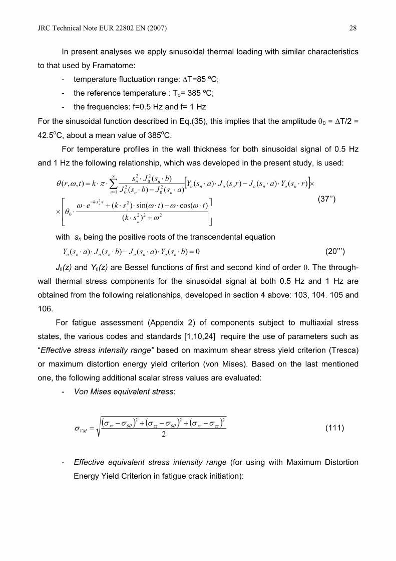
In present analyses we apply sinusoidal thermal loading with similar characteristics
to that used by Framatome:
- temperature fluctuation range: ∆T=85 ºC;
- the reference temperature : To= 385 ºC;
- the frequencies: f=0.5 Hz and f= 1 Hz
For the sinusoidal function described in Eq.(35), this implies that the amplitude θ0 = ∆T/2 =
42.5oC, about a mean value of 385oC.
For temperature profiles in the wall thickness for both sinusoidal signal of 0.5 Hz
and 1 Hz the following relationship, which was developed in the present study, is used:
[ ]
⎥⎥
⎦
⎤
⎢⎢
⎣
⎡
+⋅
⋅⋅−⋅⋅⋅+⋅⋅×
×⋅⋅⋅−⋅⋅⋅−⋅
⋅⋅⋅⋅=
⋅⋅−
∞
=∑
222
2
0
120
20
20
2
)()cos()sin()(
)()()()()()(
)(),,(
2
ωωωωω
θ
πωθ
n
n
n
skttske
rsYasJrsJasYasJbsJ
bsJsktr
tsk
nonononon nn
nn
(37’’)
with sn being the positive roots of the transcendental equation
0)()()()( =⋅⋅⋅−⋅⋅⋅ bsYasJbsJasY nononono (20’’’)
J0(z) and Y0(z) are Bessel functions of first and second kind of order 0. The through-
wall thermal stress components for the sinusoidal signal at both 0.5 Hz and 1 Hz are
obtained from the following relationships, developed in section 4 above: 103, 104. 105 and
106.
For fatigue assessment (Appendix 2) of components subject to multiaxial stress
states, the various codes and standards [1,10,24] require the use of parameters such as
“Effective stress intensity range” based on maximum shear stress yield criterion (Tresca)
or maximum distortion energy yield criterion (von Mises). Based on the last mentioned
one, the following additional scalar stress values are evaluated:
- Von Mises equivalent stress:
( ) ( ) ( )2
222zzrrzzrr
VMσσσσσσσ θθθθ −+−+−
= (111)
- Effective equivalent stress intensity range (for using with Maximum Distortion
Energy Yield Criterion in fatigue crack initiation):

JRC Technical Note EUR 22802 EN (2007) 29
( ) ( ) ( )2
222zzrrzzrr
rangeS σσσσσσ θθθθ ∆−∆+∆−∆+∆−∆=∆ (112)
The Framatome [23] fatigue analyses used the methodology from the RCC-MR code
(Design and Construction Rules for Mechanical Components of FBR Nuclear Islands), and
the plasticity effects were taken into account by means of Kυ and Kε factors (respectively
triaxiality and local plastic stress concentration effects):
( ) rangeTOT SE
KK ∆⋅+
⋅−+=∆3
)1(21 νε ευ (113)
Some comments are necessary before discussing the comparison between various
methods. The analytical solutions for the temperature distribution (Eq. 37’’) and the
associated thermal stress components (Eqs. 103’, 104’, 105’, 106’) were implemented by
means of specially written routines implemented in the MATLAB software package
(MATLAB 7.3 version, with Symbolic Math Toolbox). A first task was to establish the
number of roots needed from transcendental equation (20’’’) because the response of the
solutions become more stabile as the number of roots is increased. We used one hundred
roots and note that further increasing the number gives negligible improvement in the
predictions. This means that an equal number of the evaluations of the above equations
must be performed. Also, due to Bessel function properties, the accuracy of the analytical
solutions for both the temperature and the stress response is strongly dependent on the
size of the incremental steps in the “r” variable (radial distance through wall thickness). An
investigation was made to optimize this and it was concluded that several hundred are
required. Taking into account the complex mathematical series expansions used for the
analytical solutions for temperature distribution and thermal stress components through
the wall thickness of hollow cylinder, the solutions show some point-to-point variability and
therefore we applied a smoothing technique based on the polynomial fitting of analytical
distributions. This technique is widely applied [1,6,7,8] to facilitate the calculation of stress
intensity factors based on the thermal stresses profile [9], which are used for crack growth
assessment.
5.1 Comparison with independent studies on predicted temperature and stress distribution The temperature profile distributions through wall-thickness of hollow cylinder have
been obtained using Eq. (37’’) for sinusoidal signal frequencies of f=0.5 Hz and f= 1Hz.

JRC Technical Note EUR 22802 EN (2007) 30
In Figure 2, for f=0.5 Hz, the temperature profiles are shown for different time: t1=
0.5 sec and t2=1.5 sec (corresponding to instants of maximum deviation of the fluid
temperature from the mean or reference value) and t3=1 sec and t4= 2 sec, (minimum, i.e.
zero, deviation from the reference temperature). As can be observed, at the times of
maximum deviation, the resulting temperature field decays significantly through of pipe
wall thickness, reaching negligible values after 3 mm deep. The temperature distributions
are identical with those obtained in the Korean study [16] (see Figure 4) and by
Framatome [23] (see Figure 5). Figure 3 shows the time-dependence of temperature at
selected locations through the pipe thickness. The thermal reponse of the material has a
sinusoidal form but with a decreased amplitude corresponding to the depth in the pipe
wall. The temperature distributions calculated by NNC (Figure 6) display the same
characteristics , but in relation to 300 °C as reference temperature.
Figures 7 and 8 show the through-thickness and time dependence of the
temperature profiles for f=1 Hz. As expected, the penetration depth of the temperature
fluctuations are smaller (about 2 cm) than for f=0.5 Hz. Again the results are in good
agreement with temperature distributions obtained by Framatome for the f=1 Hz case
(Figure 9).
Calculations of the hoop, axial and radial thermal stress components have been
made for the same frequencies (f=0.5 Hz and f=1 Hz) as in the thermal analyses. The
distribution of the thermal stresses over the thickness of the wall is analyzed for a period of
2 sec in case of f=0.5 Hz and for sec for f=1Hz. In first half of each time period the
stresses are compressive at the inner surface, switching then to tensile for the second half.
Figure 10 shows the limiting hoop stress distributions for f=0.5 Hz. On inner surface
the maximum values are: σθcomp= -169.5 MPa (in compression), σθtensile= 171.5MPa (in
tension), giving a range value of ∆σθθ=341 MPa . For f=1 Hz (Figure 11) the respective
values are: σθcomp = -160 MPa, σθtensile =160 MPa, ∆σθθ= 320MPa . As expected, ∆σθθ (1
Hz) < ∆σθθ (0.5Hz). A comparison could be made with the NNC calculation [23], see
Figure 12,
For axial thermal stress component two evaluations were performed: for εzz= ε0 ( as
used by NNC) and εzz= 0 (Framatome). In the first case (Figures 13 and 14) we obtain the
following maximum values: σzcomp= -137 MPa, σztensile= 156MPa , ∆σzz =293 MPa for f=0.5
Hz and σzcomp= -137MPa, σztensile= 151 MPa , ∆σzz =288 MPa for f=1 Hz. In the εzz= 0 case
the results are: σzcomp= -160MPa, σztensile= 167MPa, ∆σzz=327 MPa and σzcomp= -153 MPa,
σztensile= 157 MPa, ∆σzz = 310 MPa for f =0.5Hz and f=1 Hz respectively (Figures 15 and

JRC Technical Note EUR 22802 EN (2007) 31
16). Using the Framatome predictions for f=0.5Hz (Figures 17 and 18), a direct
comparison with the results from the present work is made in Figure 19 (εzz= 0). For f=1 Hz
the comparison used the corresponding Framatome results given in Figures 20 and 21,
and Figure 22 shows the two sets of axial thermal stress predictions for εzz= 0. The
agreement is considered good for f=0.5Hz and very good at f=1Hz.
No predictions of radial thermal stress are reported in the NCC or Framatome
studies. In any case the present work for f=0.5 Hz and f=1Hz show that the values are too
small to have an impact on thermal fatigue assessment.
The von Mises equivalent stress profiles are displayed in Figures 25 and 26 for
f=0.5 Hz in the εzz= ε0 and εzz= 0 cases respectively. Two instants of time were chosen:
t=0.5 sec (for maximum values) and t=4 sec (for minimum values). Comparing the
Framatome calculations (Figure 27) and those of the present work, very good agreement
is obtained, as shown in Figure 28. A similar comparison for f=1 Hz was performed based
on Figures 29 and 30 (present work) and Figure 31 (Framatome calculations). The von
Mises equivalent stress profiles are in very closely agreement as can be seen in Figure 32.
From the Korean study [16] a stress intensity profile (Tresca definition) is shown in Figure
33, with a similar profile through the wall thickness.
The effective equivalent stress intensity range profile distribution has been
evaluated for both frequencies and the εzz= ε0 and εzz= 0 cases. For f=0.5 Hz (Figures 34
and 35) the results for ∆Srange.max are 307 and 328 MPa, respectively. The results for f=1
Hz are displayed in Figures 36 and 37 and the corresponding maximum ∆Srange.max values
are 275.7 and 293.4 MPa. These results confirm the frequency f=0.5 Hz is more critical
than f=1Hz from thermal fatigue point of view. Tables 1 and 2 summarise the main results
from the present work and from other reported analyses of this benchmark.
Table 1 Results for thermal stress components at f=0.5 Hz Thermal stress components Present work Framatome[23] NNC[23] Ref. [16]
Hoop stress range (MPa) ∆σθθ= 341 ∆σθθ= 310 - 186.6
Axial stress range (MPa)
εzz= ε0
εzz=0
∆σzz= 293
∆σzz= 327
-
∆σθθ= 310
-
-
211
Radial stress range (MPa) ∆σrr= 1 - - 42.6
Von Mises equivalent stress (MPa)
εzz= ε0
εzz= 0
σVMmax=152
σVMmax=163
-
- σVMmax=154
-
-
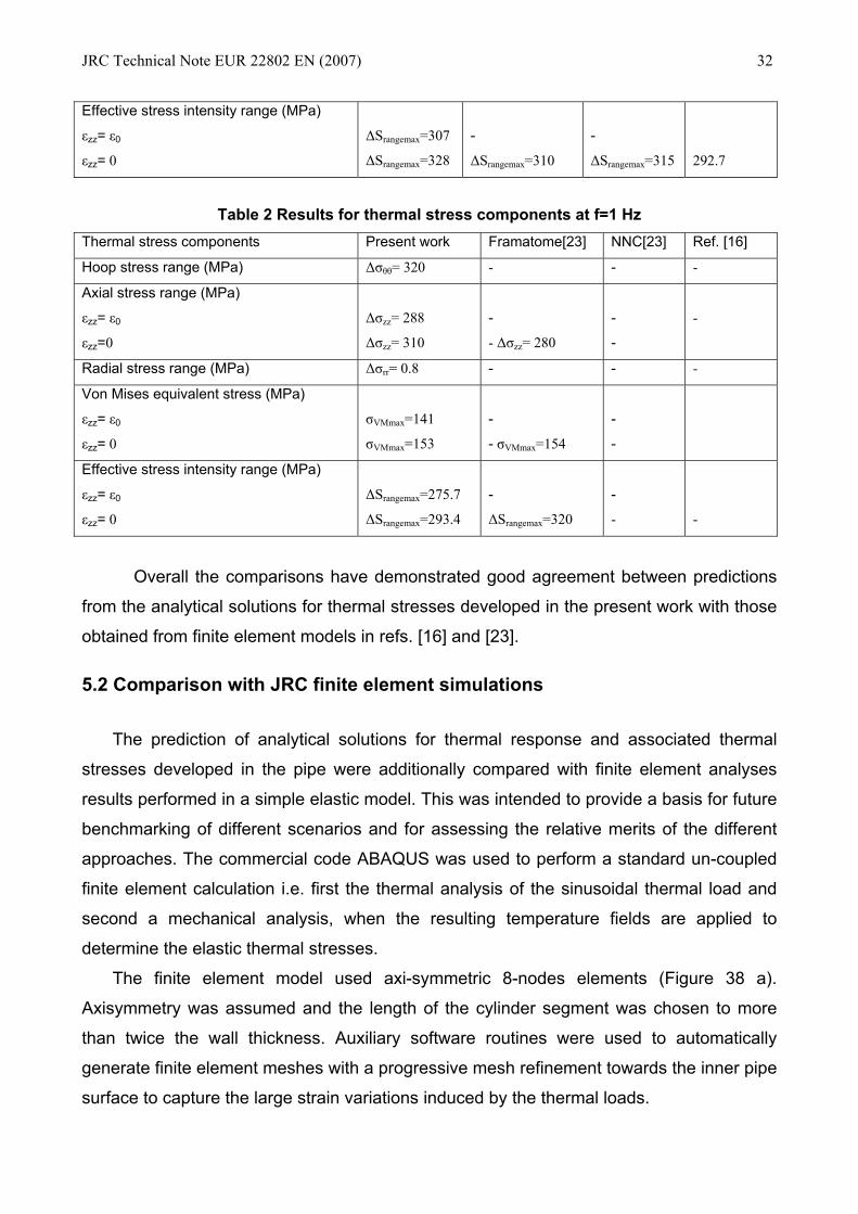
JRC Technical Note EUR 22802 EN (2007) 32
Effective stress intensity range (MPa)
εzz= ε0
εzz= 0
∆Srangemax=307
∆Srangemax=328
-
∆Srangemax=310
-
∆Srangemax=315
292.7
Table 2 Results for thermal stress components at f=1 Hz
Thermal stress components Present work Framatome[23] NNC[23] Ref. [16]
Hoop stress range (MPa) ∆σθθ= 320 - - -
Axial stress range (MPa)
εzz= ε0
εzz=0
∆σzz= 288
∆σzz= 310
-
- ∆σzz= 280
-
-
-
Radial stress range (MPa) ∆σrr= 0.8 - - -
Von Mises equivalent stress (MPa)
εzz= ε0
εzz= 0
σVMmax=141
σVMmax=153
-
- σVMmax=154
-
-
Effective stress intensity range (MPa)
εzz= ε0
εzz= 0
∆Srangemax=275.7
∆Srangemax=293.4
-
∆Srangemax=320
-
-
-
Overall the comparisons have demonstrated good agreement between predictions
from the analytical solutions for thermal stresses developed in the present work with those
obtained from finite element models in refs. [16] and [23].
5.2 Comparison with JRC finite element simulations
The prediction of analytical solutions for thermal response and associated thermal
stresses developed in the pipe were additionally compared with finite element analyses
results performed in a simple elastic model. This was intended to provide a basis for future
benchmarking of different scenarios and for assessing the relative merits of the different
approaches. The commercial code ABAQUS was used to perform a standard un-coupled
finite element calculation i.e. first the thermal analysis of the sinusoidal thermal load and
second a mechanical analysis, when the resulting temperature fields are applied to
determine the elastic thermal stresses.
The finite element model used axi-symmetric 8-nodes elements (Figure 38 a).
Axisymmetry was assumed and the length of the cylinder segment was chosen to more
than twice the wall thickness. Auxiliary software routines were used to automatically
generate finite element meshes with a progressive mesh refinement towards the inner pipe
surface to capture the large strain variations induced by the thermal loads.

JRC Technical Note EUR 22802 EN (2007) 33
Two different boundary conditions were considered:
- top edge of the sample free to expand in the axial direction, Figure 38b;
- top edge of the sample fixed in the axial direction, Figure 38c.
N.B. The model is restrained in the radial direction at the top outer edge, but this has
virtually no influence on stress distributions in the bottom radial plane, which are used for
comparison with the analytical solutions. The material properties used for elastic analyses
are mentioned in previous chapter.
The characteristic thermal sinusoidal signals applied during this analyse were similar to
those used in the analytical calculation. The reference temperature of the sample is
T0=385˚C, the temperature fluctuation range is ∆T=85˚C and the frequencies considered
are ν=0.5Hz and ν=1Hz.
The thermal sinusoidal loads have been applied at time zero at the inner wall of the
sample uniformly heated at 385˚C for t<0sec. The load was applied for 9 sec and the
temperature and stress/strain variations across the wall thickness in function of time have
been monitored.
To apply the sinusoidal load in the FE analysis the easiest option was to use the
standard Fourier series routine by means of the *AMPLITUDE keyword and its periodic
option. The amplitude, Amp, defined in this way results in:
( )[ ]∑=
−+−+=N
nnn ttnBttnAAAmp
1000 )(sincos ϖϖ for t ≥ t0 (114)
0AAmp = for t < t0 (115)
where N is the number of terms in the Fourier series, ω is the radial frequency in
rad/sec, t0 is the starting time, A0 is the constant term in the Fourier series, An=1,2…are the
first, second, etc. coefficients of the cosine terms and Bn=1,2…are the first, second, etc.
coefficients of the sine terms. In our case: N=1, A0=T0, A1=0, B1=42.5 ˚C.
Plots of the temperature field at several instants of time, during of temperature wave
propagation across the wall thickness are shown in Figure 39 for f=0.5 Hz and Figure 40
for f=1 Hz. As can be seen the temperature wave front is non-homogenous due to the
rapid fluctuation of the thermal load at the inner boundary of model.
Figures 41 and 42 show the von Mises iso-stress plots at a frequency f= 1Hz
corresponding to the point-to-point temperature fluctuations in the body of pipe, for free

JRC Technical Note EUR 22802 EN (2007) 34
and fixed boundary conditions respectively. The visible distortion (strongly magnified for
better visualization) in the latter is due to the radial constraint at the top of the model.
Before graphically comparing the results from analytical and finite element analyses
it is important to mention that in the following, the instants of time for calculating the
temperature and corresponding elastic stress components have been chosen to comply
with the time steps used in the FE analysis.
The predicted temperature profiles across the wall-thickness are shown in Figures
43 and 44 for frequencies of f=0.5 Hz and f= 1Hz. The analytical predictions fit quite well to
those from the FEA at the same instants of time.
Figures 45 and 46 show the maximum and minimum hoop thermal stresses for both
frequencies. These values correspond to a fixed edge boundary condition. In the case of
axial stress the comparison has been made for both the boundary condition cases: fixed
and free axial strains. Figures 47 to 50 confirm the good agreement between the predicted
and FE axial stress values across the wall thickness of the pipe for both the boundary
conditions. The von Mises equivalent stress comparisons are depicted in Figures 51-54.
Even though the FE stress gradients for the free axial displacement boundary condition
(εzz=ε0) are a bit higher for the analytical solutions, still the maximum values very close to
those obtained by FEA. For the fixed boundary condition both the axial stress maximum
values and the gradients are in good agreement with the FE results. The effective
equivalent stress intensity range is a very important parameter in relation to the fatigue
curves used to obtain the cumulative usage factors for fatigue crack initiation assessment.
The agreement between analytical and FEA calculations is rather good for maximum
values as well as for the stress gradient through the wall-thickness, can be seen in Figures
55-58. Table 3 summarizes the results of the above comparisons. The agreement between
analytical and FEA predictions provides verification of the analytical model developed
during this work.
Table 3 Comparison between analytical and FEA calculation for thermal stresses due to sinusoidal thermal loading f=0.5 Hz f= 1 Hz Stress component Analytical
MPa FEA MPa
Analytical MPa
FEA MPa
Hoop stress
300 280 325 308
Axial stress εzz=0 εzz=ε0
290 265
285 240
310 312
312 313
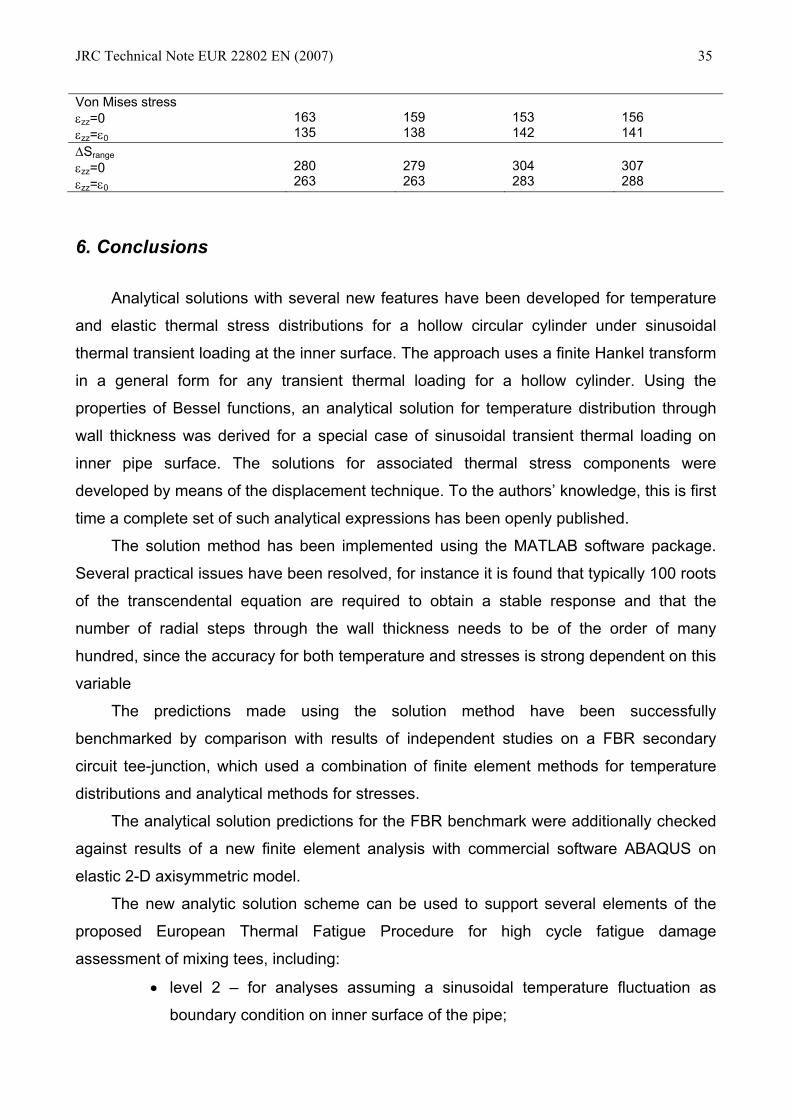
JRC Technical Note EUR 22802 EN (2007) 35
Von Mises stress εzz=0 εzz=ε0
163 135
159 138
153 142
156 141
∆Srange εzz=0 εzz=ε0
280 263
279 263
304 283
307 288
6. Conclusions
Analytical solutions with several new features have been developed for temperature
and elastic thermal stress distributions for a hollow circular cylinder under sinusoidal
thermal transient loading at the inner surface. The approach uses a finite Hankel transform
in a general form for any transient thermal loading for a hollow cylinder. Using the
properties of Bessel functions, an analytical solution for temperature distribution through
wall thickness was derived for a special case of sinusoidal transient thermal loading on
inner pipe surface. The solutions for associated thermal stress components were
developed by means of the displacement technique. To the authors’ knowledge, this is first
time a complete set of such analytical expressions has been openly published.
The solution method has been implemented using the MATLAB software package.
Several practical issues have been resolved, for instance it is found that typically 100 roots
of the transcendental equation are required to obtain a stable response and that the
number of radial steps through the wall thickness needs to be of the order of many
hundred, since the accuracy for both temperature and stresses is strong dependent on this
variable
The predictions made using the solution method have been successfully
benchmarked by comparison with results of independent studies on a FBR secondary
circuit tee-junction, which used a combination of finite element methods for temperature
distributions and analytical methods for stresses.
The analytical solution predictions for the FBR benchmark were additionally checked
against results of a new finite element analysis with commercial software ABAQUS on
elastic 2-D axisymmetric model.
The new analytic solution scheme can be used to support several elements of the
proposed European Thermal Fatigue Procedure for high cycle fatigue damage
assessment of mixing tees, including:
• level 2 – for analyses assuming a sinusoidal temperature fluctuation as
boundary condition on inner surface of the pipe;

JRC Technical Note EUR 22802 EN (2007) 36
• level 3 – for load spectrum analysis based on one-dimension temperature
and stress evaluations at each measured location;
• level 4 – providing through-thickness stress profiles for thermal fatigue crack
growth assessment.
Further work will address the integration of the solution scheme into an overall
process for determining thermal fatigue usage factors, considering also aspects as
plasticity effects and selection of fatigue life curves.

JRC Technical Note EUR 22802 EN (2007) 37
References
1. S. Chapuliot, C. Gourdin, T. Payen, J.P.Magnaud, A.Monavon, Hydro-thermal-
mechanical analysis of thermal fatigue in a mixing tee, Nuclear Engineering and
Design 235 (2005) 575-596
2. NEA/CSNI/R (2005) 8, Thermal cycling in LWR components in OECD-NEA
member countries, JT001879565
3. NEA/CSNI/R(2005)2, FAD3D –An OECD/NEA benchmark on thermal fatigue in
fluid mixing areas, JT00188033
4. IAEA-TECDOC-1361, Assessment and management of ageing of major nuclear
power plant components important to safety-primary piping in PWRs, IAEA, July
2003
5. Lin-Wen Hu, Jeongik Lee, Pradip Saha, M.S.Kazimi, Numerical Simulation study of
high thermal fatigue caused by thermal stripping, Third International Conference on
Fatigue of Reactor Components, Seville, Spain 3-6 October 2004,
NEA/CSNI/R(2004)21
6. Brian B. Kerezsi, John W.H. Price, Using the ASME and BSI codes to predict crack
growth due to repeated thermal shock, International Journal of Pressure Vessels
and Piping 79 (2002) 361-371
7. C. Faidy RSE-M. A general presentation of the French codified flaw evaluation
procedure, International Journal of Pressure Vessel and Piping 77 (2000) 919-927
8. T. Wakai, M. Horikiri, C. Poussard, B. Drubay A comparison between Japanese
and French A 16 defect assessment procedures for thermal fatigue crack growth,
Nuclear Engineering and Design 235 (2005) 937-944
9. A.R. Shahani, S.M. Nabavi, Transient thermal stress intensity factors for an internal
longitudinal semi-elliptical crack in a thick-walled cylinder, Engineering Fracture
Mechanics (2007), doi:101016/j.engfrachmech.2006.11.018
10. API 579 Fitness-for-Service-API Recommended Practice 579, First Edition,
January 2000, American Petroleum Institute
11. B.A. Boley, J. Weiner, Theory of Thermal Stresses, John Wiley & Sons, 1960
12. N. Noda, R.B. Hetnarski, Y. Tanigawa, Thermal Stresses, 2nd Ed., Taylor &
Francis, 2003

JRC Technical Note EUR 22802 EN (2007) 38
13. S.P. Timoshenko, J.N. Goodier, Theory of Elasticity, McGraw-Hill, New York,
(1987)
14. A.E. Segal, Transient analysis of thick-walled piping under polynomial thermal
loading, Nuclear Engineering and Design 226 (2003) 183-191
15. H.-Y. Lee, J.-B. Kim, B. Yoo Green’s function approach for crack propagation
problem subjected to high cycle thermal fatigue loading, International Journal of
Pressure Vessel and Piping 76 (1999) 487-494
16. H.-Y.Lee, J.-B. Kim, B. Yoo Tee-Junction of LMFR secondary circuit involving
thermal, thermomechanical and fracture mechanics assessment on a stripping
phenomenon, IAEA-TECDOC-1318, “Validation of fast reactor thermomechanical
and thermohydraulic codes”, Final report of a coordinated research project 1996-
1999 (1999)
17. A.R. Shahani, S.M. Nabavi, Analytical solution of the quasi-static thermoelasticity
problem in a pressurized thick-walled cylinder subjected to transient thermal
loading, Applied Mathematical Modelling (2006), doi:10.1016/j.apm.2006.06.008
18. S. Marie, Analytical expression of the thermal stresses in a vessel or pipe with
cladding submitted to any thermal transient, International Journal of Pressure
Vessel and Piping 81 (2004) 303-312
19. K.-S. Kim , N. Noda, Green’s function approach to unsteady thermal stresses in an
infinite hollow cylinder of functionally graded material, Acta Mechanica 156, 145-
161 (2000)
20. N.T. Eldabe, M. El-Shahed, M. Shawkey , An extension of the finite Hankel
transform, Applied Mathematics and Computations 151 (2004) 713-717
21. I.N. Sneddon, The Use of Integral Transforms, McGraw-Hill, New York, (1993)
22. M. Garg, A.Rao, S.L. Kalla, On a generalized finite Hankel transform, Applied
Mathematics and Computation (2007), doi:10.1016/j.amc.2007.01.076
23. D. Buckthorpe, O. Gelineau, M.W.J. Lewis, A. Ponter, Final report on CEC study
on thermal stripping benchmark –thermo mechanical and fracture calculation,
Project C5077/TR/001, NNC Limited 1988
24. O.K. Chopra, W.J. Shack, Effect of LWR Coolant Environments on the fatigue Life
of reactor Materials, Draft report for Comment, NUREG/CR-6909, ANL 06/08, July
2006, U.S. Nuclear Regulatory Commission , Office of Nuclear Regulatory
Research, Washington, DC

JRC Technical Note EUR 22802 EN (2007) 39
FIGURES

JRC Technical Note EUR 22802 EN (2007) 40

JRC Technical Note EUR 22802 EN (2007) 41
Figure 1. Geometrical characteristics of the components in the tee junction area

JRC Technical Note EUR 22802 EN (2007) 42
0.247 0.248 0.249 0.25 0.251 0.252 0.253 0.254340
350
360
370
380
390
400
410
420
430
Radial distance m
Tem
pera
ture
C
Temperature profile through thickness for f=0.5Hz
t=0.5 sect=1 sect=1.5 sect=2 sec
Figure 2 Temperature profile distribution through wall-thickness of hollow cylinder
at various moments of time, f=0.5 Hz NB: ri=0.247 m, inner surface of pipe; re=0.247 m, outer surface of pipe
0 0.5 1 1.5 2 2.5 3 3.5 4340
350
360
370
380
390
400
410
420
430
Time sec
Tem
pera
ture
C
Time-dependence of temperature in specified locations of thickness,f=0.5 Hz
r=0.247 mr=0.248 mr=0.250 mr=0.253 m
Figure 3 Time-dependence of temperature in some locations of wall-thickness
for frequency f=0.5 Hz

JRC Technical Note EUR 22802 EN (2007) 43
Figure 4. Temperature profile along the thickness direction for sinusoidal loading, f= 0.5 Hz [16]
Figure 5. Framatome calculations: Temperature profile for f= 0.5 Hz sinusoidal signal [23]

JRC Technical Note EUR 22802 EN (2007) 44
Figure 6. NNC calculations: Typical temperature results using filtered AEA TC01A data -Temperature variation through thickness over time period 20.2 s to 20.9 sec [23]
0.247 0.248 0.249 0.25 0.251 0.252 0.253 0.254340
350
360
370
380
390
400
410
420
430
Radial distance m
Tem
pera
ture
C
Temperature profile through thickness, f=1 Hz
t=0.25 sect=0.5 sect=0.75 sect=1 sec
Figure 7. Temperature profile distribution through wall-thickness of hollow cylinder at various moments of time for frequency f=1 Hz

JRC Technical Note EUR 22802 EN (2007) 45
0 0.2 0.4 0.6 0.8 1 1.2 1.4 1.6 1.8 2340
350
360
370
380
390
400
410
420
430
Time sec
Tem
pera
ture
C
Time-dependence of temperature in specified locations of thickness,f=1 Hz
r=0.247 mr=0.248 mr=0.250 mr=0.253 m
Figure 8. Time-dependence of temperature in some locations of wall-thickness for frequency f=1 Hz
Figure 9. Framatome calculations: Temperature profile for f= 1 Hz sinusoidal signal
[23]

JRC Technical Note EUR 22802 EN (2007) 46
0.247 0.248 0.249 0.25 0.251 0.252 0.253 0.254 0.255 0.256-200
-150
-100
-50
0
50
100
150
200
Radial distance m
Hoo
p st
ress
MP
a
The hoop stress profile at max values, f=0.5 Hz
0.5 sec1.5 sec
Figure 10. The hoop stress profile distributions through wall thickness of hollow cylinder for instants with extreme values, for f=0.5 Hz
(σcomp= -169.5 MPa, σtensile= 171.5MPa, ∆σθθ=341 MPa )
0.247 0.248 0.249 0.25 0.251 0.252 0.253 0.254-200
-150
-100
-50
0
50
100
150
200
Radial distance m
Hoo
p st
ress
MP
a
The hoop stress profile at max values, f=1Hz
0.25 sec0.75 sec
Figure 11. The hoop stress profile distribution through wall thickness of hollow cylinder for instants with extreme values, for f=1 Hz (σcomp= -160 MPa, σtensile=160 MPa, ∆σθθ= 320MPa )

JRC Technical Note EUR 22802 EN (2007) 47
Figure 12. NNC calculations: Axial and hoop stress variation through thickness over time period 20.2 to 20.85 sec for filtered AEA data at position TC01A [23]
0.247 0.248 0.249 0.25 0.251 0.252 0.253 0.254-150
-100
-50
0
50
100
150
200
Radial distance m
Axi
al s
tress
MP
a
The axial stress profile at max values,f=0.5Hz,eps=E0 ,
0.5 sec1.5 sec
Figure 13. The axial stress profile distributions (εzz=ε0 ) through wall thickness of hollow cylinder for instants with minimum and maximum values, for f=0.5 Hz
(σcomp= -137 MPa, σtensile= 156MPa , ∆σzz =293 MPa )

JRC Technical Note EUR 22802 EN (2007) 48
0.247 0.248 0.249 0.25 0.251 0.252 0.253 0.254-150
-100
-50
0
50
100
150
200
Radial distance m
Axi
al s
tress
MP
a
p , , p ,
0.25 sec0.75 sec
Figure 14. The axial stress profile distribution (εzz=ε0 ) through wall thickness of hollow cylinder for instants with minimum and maximum values, for f=1 Hz (σcomp= -137MPa, σtensile= 151 MPa ,
∆σzz =288 MPa )
0.247 0.248 0.249 0.25 0.251 0.252 0.253 0.254-200
-150
-100
-50
0
50
100
150
200
Radial distance m
Axi
al s
tress
MP
a
0.5 sec1.5 sec
Figure 15. The axial stress profile distributions (εzz=0) through wall thickness of a hollow cylinder for instants with minimum and maximum values, for f=0.5 Hz (σcomp= -160MPa, σtensile= 167MPa,
∆σzz=327 MPa )

JRC Technical Note EUR 22802 EN (2007) 49
0.247 0.248 0.249 0.25 0.251 0.252 0.253 0.254-200
-150
-100
-50
0
50
100
150
200
Radial distance m
Axi
al s
tress
MP
a
The axial stress profile at max values, f=1 Hz, epsZ=0
0.25 sec0.75 sec
Figure 16. The axial stress profile distributions (εzz=0 ) through wall thickness of
hollow cylinder for instants with minimum and maximum values, for f=1 Hz (σcomp= -153 MPa, σtensile= 157 MPa , ∆σzz = 310 MPa )
Figure 17 Framatome calculations: Axial stress profile, f=0.5 KHz sinusoidal signal (εzz=0) [23]
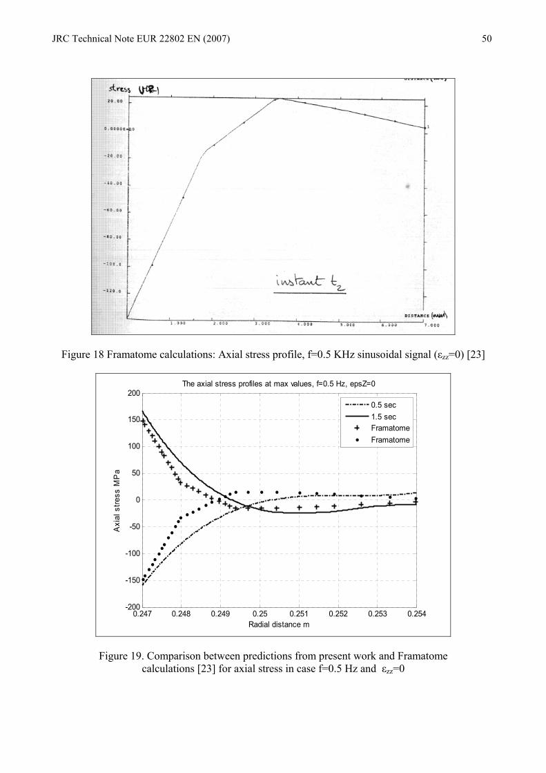
JRC Technical Note EUR 22802 EN (2007) 50
Figure 18 Framatome calculations: Axial stress profile, f=0.5 KHz sinusoidal signal (εzz=0) [23]
0.247 0.248 0.249 0.25 0.251 0.252 0.253 0.254-200
-150
-100
-50
0
50
100
150
200
Radial distance m
Axi
al s
tress
MP
a
The axial stress profiles at max values, f=0.5 Hz, epsZ=0
0.5 sec1.5 secFramatomeFramatome
Figure 19. Comparison between predictions from present work and Framatome calculations [23] for axial stress in case f=0.5 Hz and εzz=0

JRC Technical Note EUR 22802 EN (2007) 51
Figure 20 Framatome calculations: Axial stress profile, f=1 Hz sinusoidal signal (εzz=0) [23]
Figure 21 Framatome calculations: Axial stress profile, f=1 Hz sinusoidal signal (εzz=0)[23]

JRC Technical Note EUR 22802 EN (2007) 52
0.247 0.248 0.249 0.25 0.251 0.252 0.253 0.254-200
-150
-100
-50
0
50
100
150
200
Radial distance m
Axi
al s
tress
MP
a
The axial stress profiles, f=1 Hz, epsZ=0
0.25 sec0.75 sec+ Framatome+ Framatome
Figure 22 Comparison between predictions from present work and Framatome
calculations [23] for axial stress in case f=1 Hz and εzz=0
0.247 0.248 0.249 0.25 0.251 0.252 0.253 0.254-0.8
-0.6
-0.4
-0.2
0
0.2
0.4
0.6
Radial distance m
Rad
ial s
tress
MP
a
The radial stress profile at max values, f=0.5 Hz
0.5 sec1.5 sec
Figure 23. The radial stress profile distributions through wall thickness of
hollow cylinder for instants with minimum and maximum values, for f=0.5 Hz (σmin= -0.5MPa, σmax= 0.5MPa, ∆σrr=1 MPa )
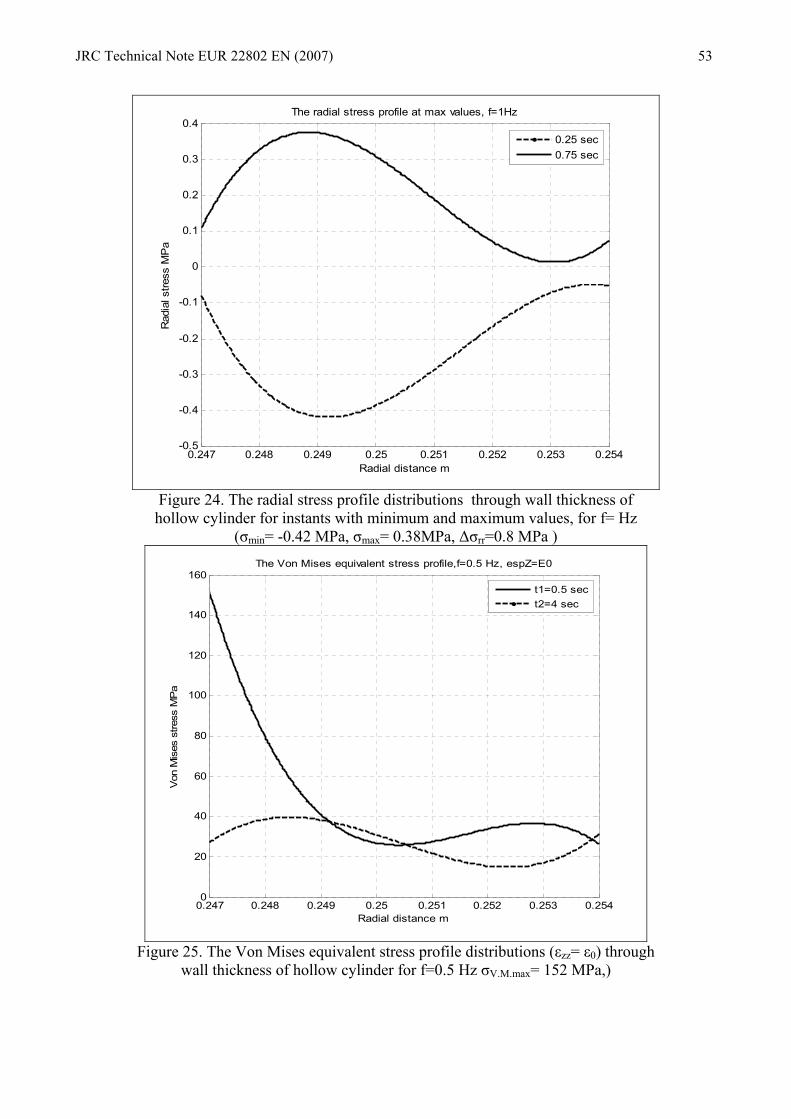
JRC Technical Note EUR 22802 EN (2007) 53
0.247 0.248 0.249 0.25 0.251 0.252 0.253 0.254-0.5
-0.4
-0.3
-0.2
-0.1
0
0.1
0.2
0.3
0.4
Radial distance m
Rad
ial s
tress
MP
a
The radial stress profile at max values, f=1Hz
0.25 sec0.75 sec
Figure 24. The radial stress profile distributions through wall thickness of hollow cylinder for instants with minimum and maximum values, for f= Hz
(σmin= -0.42 MPa, σmax= 0.38MPa, ∆σrr=0.8 MPa )
0.247 0.248 0.249 0.25 0.251 0.252 0.253 0.2540
20
40
60
80
100
120
140
160
Radial distance m
Von
Mis
es s
tress
MP
a
The Von Mises equivalent stress profile,f=0.5 Hz, espZ=E0
t1=0.5 sect2=4 sec
Figure 25. The Von Mises equivalent stress profile distributions (εzz= ε0) through
wall thickness of hollow cylinder for f=0.5 Hz σV.M.max= 152 MPa,)

JRC Technical Note EUR 22802 EN (2007) 54
0.247 0.248 0.249 0.25 0.251 0.252 0.253 0.254-20
0
20
40
60
80
100
120
140
160
180
Radial distance m
Von
Mis
es s
tress
MP
a
The Von Mises equivalent stress profile,f=0.5 Hz,espZ=0
t1=0.25 sect2=4 sec
Figure 26. The Von Mises equivalent stress profile distribution (εzz= 0) through
wall thickness of hollow cylinder for f=0.5 Hz, σV.M.max= 163 MPa
Figure 27 Framatome calculations [23]: Von Mises profile 0.5 Hz
sinusoidal signal (εzz=0)

JRC Technical Note EUR 22802 EN (2007) 55
0.247 0.248 0.249 0.25 0.251 0.252 0.253 0.2540
20
40
60
80
100
120
140
160
180
Radial distance m
Von
Mis
es s
tress
MP
a
The Von Mises equivalent stress profile,f=0.5 Hz, espZ=0
t1=0.5 secFramatome
Figure 28 Comparison between predictions from present work and Framatome
calculations for Von Mises equivalent stress profile, f=0.5 Hz, εzz=0
0.247 0.248 0.249 0.25 0.251 0.252 0.253 0.2540
50
100
150
Radial distance m
Von
Mis
es s
tress
MP
a
The Von Mises equivalent stress profiles, f=1 Hz, espZ=E0
t1=0.25 sect2=4 sec
Figure 29. The Von Mises equivalent stress profiles distribution (εzz= ε0) through
wall thickness of hollow cylinder, f=1 Hz, σV.M.max= 141 MPa

JRC Technical Note EUR 22802 EN (2007) 56
0.247 0.248 0.249 0.25 0.251 0.252 0.253 0.254-20
0
20
40
60
80
100
120
140
160
Radial distance m
Von
Mis
es s
tress
MP
a
Time-dep of Von Mises Stress for f=1 Hz and espZ=0
t1=0.25 sect2=4 sec
Figure 30. The Von Mises equivalent stress profiles distribution (εzz= 0) through
wall thickness of hollow cylinder for f=1 Hz, σV.M.max= 152 MPa
Figure 31 Framatome calculations [23]: Von Mises profile 1 Hz sinusoidal signal (εzz=0)

JRC Technical Note EUR 22802 EN (2007) 57
0.247 0.248 0.249 0.25 0.251 0.252 0.253 0.2540
20
40
60
80
100
120
140
160
Radial distance m
Von
Mis
es s
tress
MP
a
The Von Mises equivalent stress profiles,f=1 Hz ,espZ=0
t1=0.25 secFramatome
Figure 32. Comparison between profile predictions from present work and Framatome calculations
[23] for Von Mises equivalent stress, f=1 Hz, εzz=0
Figure 33 Stress intensity profile (Tresca) along thickness=0.5 Hz [16]

JRC Technical Note EUR 22802 EN (2007) 58
0.247 0.248 0.249 0.25 0.251 0.252 0.253 0.2540
50
100
150
200
250
300
350
Radial distance m
Effe
ctiv
e S
tress
Inte
nsity
Ran
ge M
Pa
The effective equivalent stress intensity range profile,f=0.5 Hz,espZ=E0
Figure 34. The effective equivalent stress intensity range profile distribution
(εzz= ε0) through wall thickness of hollow cylinder for f=0.5 Hz, ∆Srange.max= 307 MPa
0.247 0.248 0.249 0.25 0.251 0.252 0.253 0.2540
50
100
150
200
250
300
350
Radial distance m
Effe
ctiv
e S
tress
s In
tens
ity R
ange
MP
a
The effective equivalent stress intensity range profile,f=0.5Hz,espZ=0)
Figure 35. The effective equivalent stress intensity range profile distribution
(εzz=0) through wall thickness of hollow cylinder for f=0.5 Hz, ∆Srange.max= 328 MPa
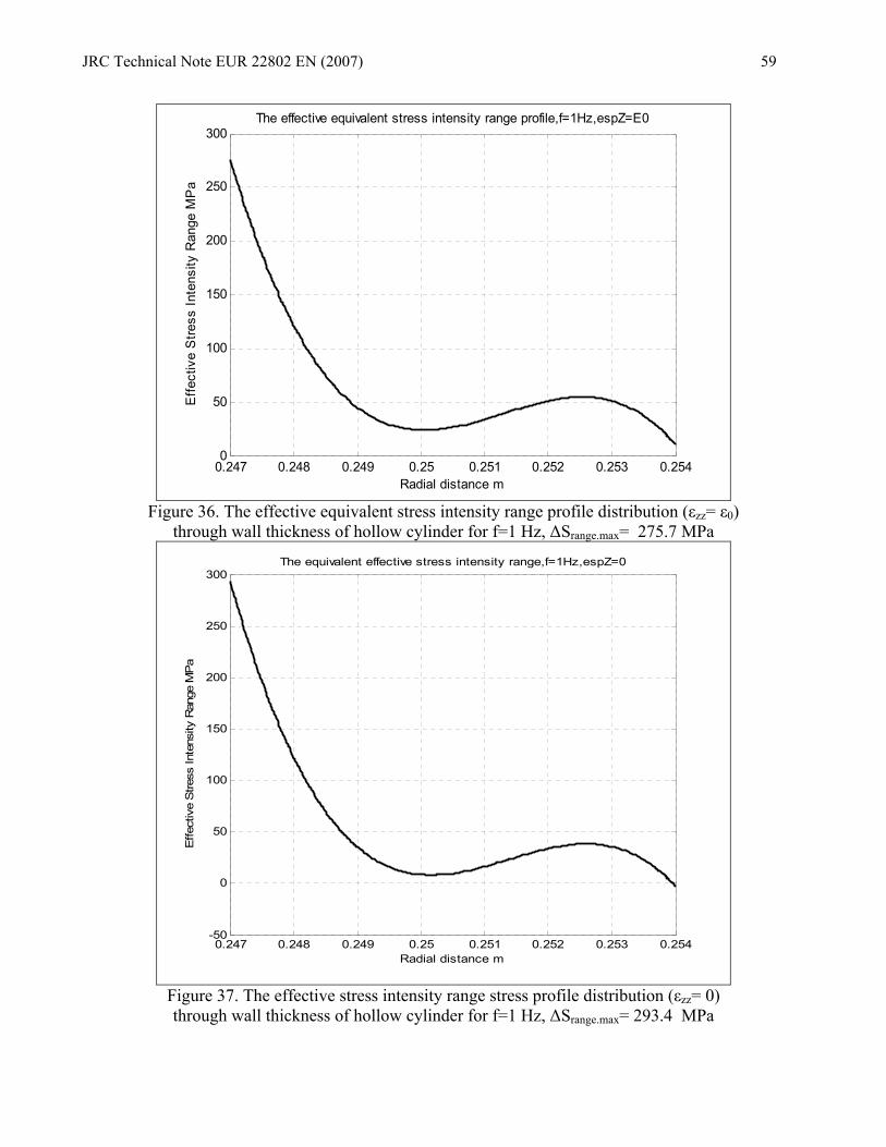
JRC Technical Note EUR 22802 EN (2007) 59
0.247 0.248 0.249 0.25 0.251 0.252 0.253 0.2540
50
100
150
200
250
300
Radial distance m
Effe
ctiv
e S
tress
Inte
nsity
Ran
ge M
Pa
The effective equivalent stress intensity range profile,f=1Hz,espZ=E0
Figure 36. The effective equivalent stress intensity range profile distribution (εzz= ε0)
through wall thickness of hollow cylinder for f=1 Hz, ∆Srange.max= 275.7 MPa
0.247 0.248 0.249 0.25 0.251 0.252 0.253 0.254-50
0
50
100
150
200
250
300
Radial distance m
Effe
ctiv
e S
tress
Inte
nsity
Ran
ge M
Pa
The equivalent effective stress intensity range,f=1Hz,espZ=0
Figure 37. The effective stress intensity range stress profile distribution (εzz= 0) through wall thickness of hollow cylinder for f=1 Hz, ∆Srange.max= 293.4 MPa

JRC Technical Note EUR 22802 EN (2007) 60
a)
b) c)
Figure 38. a) Abaqus model mesh; b) sample free to expand in the vertical direction (εzz= ε0); c) sample fixed in the vertical direction (εzz= 0).

JRC Technical Note EUR 22802 EN (2007) 61
Figure 39. Evolution of the temperature across the wall thickness for ν=0.5Hz (t=0 sec; 0.55
sec; 1.052 sec; 2.257 sec; 9 sec).

JRC Technical Note EUR 22802 EN (2007) 62
Figure 40. Evolution of the temperature across the wall thickness for ν=1Hz
(t=0 sec; 0.17 sec; 1.166 sec; 1.583 sec; 4.09 sec; 6.55 sec).

JRC Technical Note EUR 22802 EN (2007) 63
Figure 41. Evolution of the von Mises stress across the wall thickness for ν=1Hz and sample free to expand in the axial direction (εzz= ε0) (t=0.002 sec; 0.114 sec; 1.313 sec; 5.313 sec;
6.813 sec; 9 sec)

JRC Technical Note EUR 22802 EN (2007) 64
Figure 42. Evolution of the von Mises stress across the wall thickness for ν=1Hz sample fixed in the axial direction (εzz= 0),( t=0.002 sec; 0.114 sec; 1.313 sec; 6.313 sec)

JRC Technical Note EUR 22802 EN (2007) 65
0.247 0.248 0.249 0.25 0.251 0.252 0.253 0.254340
350
360
370
380
390
400
410
420
430
Radial distance (m)
Tem
pera
ture
(C)
Comparison of the temperature profiles through thickness,f=0.5Hz
t=0.65 sect=3.46 secFEAFEA
Figure 43. Comparison of temperature profiles predictions: analytical versus FEA,
f=0.5 Hz
0.247 0.248 0.249 0.25 0.251 0.252 0.253 0.254340
350
360
370
380
390
400
410
420
430
Radial distance (m)
Tem
pera
ture
(C)
Comparison of the temperature profiles through thickness,f=1 Hz
t=2.2 sect=1.8 secFEAFEA
Figure 44. Comparison of temperature profiles predictions: analytical versus FEA,
f=1.0 Hz
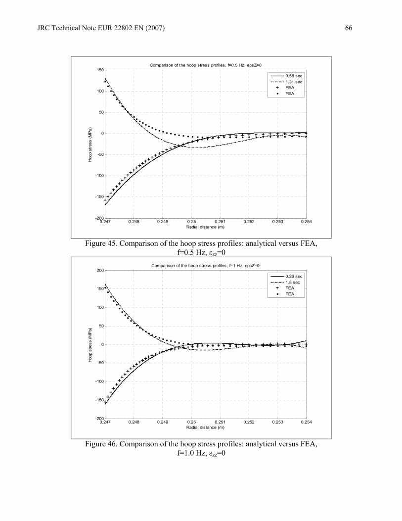
JRC Technical Note EUR 22802 EN (2007) 66
0.247 0.248 0.249 0.25 0.251 0.252 0.253 0.254-200
-150
-100
-50
0
50
100
150
Radial distance (m)
Hoo
p st
ress
(MP
a)
Comparison of the hoop stress profiles, f=0.5 Hz, epsZ=0
0.58 sec1.31 secFEAFEA
Figure 45. Comparison of the hoop stress profiles: analytical versus FEA,
f=0.5 Hz, εzz=0
0.247 0.248 0.249 0.25 0.251 0.252 0.253 0.254-200
-150
-100
-50
0
50
100
150
200
Radial distance (m)
Hoo
p st
ress
(MP
a)
Comparison of the hoop stress profiles, f=1 Hz, epsZ=0
0.26 sec1.8 secFEAFEA
Figure 46. Comparison of the hoop stress profiles: analytical versus FEA,
f=1.0 Hz, εzz=0

JRC Technical Note EUR 22802 EN (2007) 67
0.247 0.248 0.249 0.25 0.251 0.252 0.253 0.254-200
-150
-100
-50
0
50
100
150
Radial distance (m)
Axi
al s
tress
(MP
a)
Comparison of the axial stress profiles, f=0.5 Hz, epsZ=0
0.58 sec1.3 secFEAFEA
Figure 47. Comparison of the axial stress profiles: analytical versus FEA,
f=0.5 Hz, εzz=0
0.247 0.248 0.249 0.25 0.251 0.252 0.253 0.254-200
-150
-100
-50
0
50
100
150
200
Radial distance (m)
Axi
al s
tress
(MP
a)
Comparison of the axial stress profiles, f=1 Hz, epsZ=0
0.26 sec1.8 secFEAFEA
Figure 48. Comparison of the axial stress profiles: analytical versus FEA,
f=1.0 Hz, εzz=0

JRC Technical Note EUR 22802 EN (2007) 68
0.247 0.248 0.249 0.25 0.251 0.252 0.253 0.254-150
-100
-50
0
50
100
150
Radial distance (m)
Axi
al s
tress
(MP
a)
Comparison of the axial stress profiles, f=0.5 Hz, epsZ=E0
0.58 sec1.3 secFEAFEA
Figure 49. Comparison of the axial stress profiles: analytical versus FEA,
f=0.5 Hz, εzz=ε0
0.247 0.248 0.249 0.25 0.251 0.252 0.253 0.254-200
-150
-100
-50
0
50
100
150
200
Radial distance (m)
Axi
al s
tress
(MP
a)
Comparison of the axial stress profiles, f=1 Hz, epsZ=E0
0.26 sec1.8 secFEAFEA
Figure 50 . Comparison of the axial stress profiles: analytical versus FEA,
f=1.0 Hz, εzz=ε0

JRC Technical Note EUR 22802 EN (2007) 69
0.247 0.248 0.249 0.25 0.251 0.252 0.253 0.2540
20
40
60
80
100
120
140
160
180
Radial distance (m)
Von
Mis
es s
tress
(M)P
a
Comparison for Von Mises equivalent stress profiles, f=0.5 Hz, espZ=0
t1=0.58 secFEA
Figure 51. Comparison of the von Mises equivalent stress profiles: analytical versus FEA,
f=0.5 Hz, εzz =0
0.247 0.248 0.249 0.25 0.251 0.252 0.253 0.2540
20
40
60
80
100
120
140
Radial distance (m)
Von
Mis
es s
tress
(M)P
a
Comparison for Von Mises equivalent stress,f=0.5 Hz, espZ=E0
t1=0.388 secFEA
Figure 52. Comparison of the von Mises equivalent stress profiles: analytical versus FEA,
f=0.5 Hz, εzz =ε0

JRC Technical Note EUR 22802 EN (2007) 70
0.247 0.248 0.249 0.25 0.251 0.252 0.253 0.2540
20
40
60
80
100
120
140
160
Radial distance (m)
Von
Mis
es s
tress
(MP
a)
Comparison for Von Mises equivalent stress profiles ,f=1 Hz ,espZ=0
t1=0.25 secFEA
Figure 53. Comparison of the von Mises equivalent stress profiles: analytical versus FEA,
f=1.0 Hz, εzz=0
0.247 0.248 0.249 0.25 0.251 0.252 0.253 0.2540
50
100
150
Radial distance (m)
Von
Mis
es s
tress
(MP
a)
Comparison for Von Mises equivalent stress ,f=1 Hz ,espZ=E0
t1=0.258 secFEA
Figure 54. Comparison of the von Mises equivalent stress profiles: analytical versus FEA,
f=1.0 Hz, εzz=ε0

JRC Technical Note EUR 22802 EN (2007) 71
0.247 0.248 0.249 0.25 0.251 0.252 0.253 0.2540
50
100
150
200
250
300
Radial distance (m)
The
effe
ctiv
e eq
uiva
lent
stre
sss
inte
nsity
rang
e (M
Pa)
Comparison of effective equivalent stress intensity range ,f=0.5Hz,espZ=0)
AnalyticalFEM
Figure 55. Comparison of the effective equivalent stress intensity range between
instants t1=0.58 sec and t2=1.3 sec : analytical versus FEA f=0.5 Hz, εzz=0
0.247 0.248 0.249 0.25 0.251 0.252 0.253 0.2540
50
100
150
200
250
300
Radial distance (m)
The
effe
ctiv
e eq
uiva
lent
stre
sss
inte
nsity
rang
e (M
Pa)
Comparison of effective equivalent stress intensity range ,f=0.5Hz,espZ=E0)
AnalyticalFEA
Figure 56. Comparison of the effective equivalent stress intensity range between
instants t1=0.58 sec and t2=1.3 sec: analytical versus FEA f=0.5 Hz, εzz=ε0

JRC Technical Note EUR 22802 EN (2007) 72
0.247 0.248 0.249 0.25 0.251 0.252 0.253 0.2540
50
100
150
200
250
300
350
Radial distance (m)
The
effe
ctiv
e eq
uiva
lent
stre
sss
inte
nsity
rang
e (M
Pa)
Comparison of effective equivalent stress intensity range ,f=1 Hz,espZ=0)
AnalyticalFEA
Figure 57. Comparison of the effective equivalent stress intensity range between
instants t1=0.26 sec and t2=1.8 sec: analytical versus FEA f=1.0 Hz, εzz=0
0.247 0.248 0.249 0.25 0.251 0.252 0.253 0.2540
50
100
150
200
250
300
Radial distance (m)
The
effe
ctiv
e eq
uiva
lent
stre
sss
inte
nsity
rang
e (M
Pa)
Comparison of effective equivalent stress intensity range ,f=1 Hz,espZ=E0)
AnalyticalFEA
Figure 58. Comparison of the effective equivalent stress intensity range between
instants t1=0.26 sec and t2=1.8 sec: analytical versus FEA f=1.0 Hz, εzz=ε0

JRC Technical Note EUR 22802 EN (2007) 73
APPENDICES

JRC Technical Note EUR 22802 EN (2007) 74

JRC Technical Note EUR 22802 EN (2007) 75
Appendix 1: Some properties of Bessel functions
The differential equation
0)(1)(1)(2
2
2
2
=⋅⎟⎟⎠
⎞⎜⎜⎝
⎛−+⋅+ zf
zdzzdf
zdzzfd υ (A1.1)
is a Bessel’s differential equation of order υ. The first solution is expressed by
m
m
m zmm
zJ2
0 2)1(!)1()(
+∞
=∑ ⎟
⎠⎞
⎜⎝⎛⋅
++Γ−
=υ
υ υ (A1.2)
and is called a Bessel function of the first kind of order υ, where Γ is the gamma
function defined by
∫∞
−− ⋅=Γ0
1)( dttex xt for x>0 (A1.3)
The second solution of the Bessel equation which is available for all values of υ is
expressed by
)sin()()cos()()(
υπυπ υυ
υzJzJzY −−⋅
= (A1.4)
and is called the Bessel function of the second kind of order υ. If υ is not an integer,
Jυ(z) may be used instead of Yυ(z) as a second solution. Functions Jυ(z) and J-υ(z) are
independent solutions of Eq. (A1.1). When υ is an integer n, J-υ(z) is dependent on Jυ(z)
)()1()( zJzJ nn
n −−= (A1.5)
The complete solution of Eq. (A1.1) is
)()()( zYBzJAzf υυ ⋅+⋅= for all values of υ (A1.6)
)()()( zYBzJAzf nn ⋅+⋅= for an integer n (A1.7)
)()()( zJBzJAzf υυ −⋅+⋅= for non-integer υ (A1.8)
Some formulas of the Bessel functions are listed as follows

JRC Technical Note EUR 22802 EN (2007) 76
)()()(211 zJzJzJ
z +− += υυυυ (A1.9)
[ ] )()()()()()(21))
1111 zJz
zJzJz
zJzJzJdz
zdJυυυυυυ
υ υυ+−=−=−= +−+− (A1.10)
[ ] )()( 1 azJzazaJzdzd
−⋅⋅=⋅⋅ υυ
υυ (A1.11)
[ ] )()( 1 azJzazaJzdzd
+−− ⋅⋅−=⋅⋅ υυ
υυ (A1.12)
)()1()()1()( zJzJzJ nn
nn
n −−=−= − (A1.13)
zzYzJzYzJ
πυυυυ2)()()()( 11 =⋅−⋅ ++ (A1.14)
The above formulas, except for the last, are satisfied by Yυ(z) instead Jυ(z).

JRC Technical Note EUR 22802 EN (2007) 77
Appendix 2: Fatigue Evaluation Procedure Based on Elasticity Calculated Stress Results (API 579/2000) A quantity known as the “equivalent intensity of combined stress” or “stress
intensity” is computed at certain locations on the component or structure of interest. The
stress intensity at a point is a measure of stress, calculated from stress components
utilizing a yield criterion, which can be used for comparison with the mechanical strength
properties of the material obtained in tests under uniaxial load.
The “Maximum Distortion Energy Yield Criterion” may be used to establish stress
intensity. In this case the stress intensity is equal to the von Mises equivalent stress:
( ) ( ) ( )2
213
232
221 σσσσσσσ −+−+−
== vonMisesS (A2.1)
Although this yield criterion is more complicated to apply when manual calculations
are performed, it is the most common criterion for yield used in finite element analysis, and
is generally recognized to give more accurate results than the maximum shear stress yield
criterion.
Fatigue Evaluation Procedure Based on Elasticity Calculated Stress Results
A fatigue evaluation should be performed if the component is subject to cyclic
operation. The evaluation for fatigue is made on the basis of the number of applied cycles
of a stress or strain range at a point in the component. The allowable number of cycles
should be adequate for the specified duration of operation to determine the suitability for
continued operation. Fatigue curves are typically presented in two forms: fatigue curves
that are based on smooth bar test specimens and fatigue curves that are based on the test
specimens which include weld details. The stresses and strains produced by any load or
thermal condition which does not vary during the cycle need not be considered in a fatigue
analysis if the fatigue curves utilized in the evaluation are adjusted for mean stresses and
strains.
An effective total stress intensity amplitude is used to evaluate the fatigue damage
for results obtained from a linear elastic stress analysis. The effective peak stress intensity
amplitude is defined as one-half the effective total stress intensity range, calculated for
each cycle described in the loading history. The procedure can be used for the general
case where the principal stress directions change during the loading cycle.
The steps required for thermal fatigue crack initiation are described in the following:

JRC Technical Note EUR 22802 EN (2007) 78
Step1. -Determine a load history based on the past operation and future planned
operation. The load history should include all significant operating loads and events which
the component will be subjected to.
Step 2. – For a location in the component under evaluation, compute the stress
components σij and the equivalent stress for each point in the load histogram. Use this
information to create an effective stress load histogram.
Step 3. – Determine the cyclic stress range based on the effective stress histogram
developed in Step 2 using the cycle counting method in ASME E 1049 (rainflow method).
Step 4. Determine the stress tensor at the start and end points for the “kth” cycle in
the effective stress histogram counted in Step 3. Using these data, determine the stress
range and designate this quantity as ∆ σijk.
Step 5. – Compute an effective stress intensity range for the “kth” cycle using the
“Maximum Distortion Energy Yield Criterion”. Using the change in stress components
determined in Step 4, compute the effective equivalent stress intensity range for the
cycle:
( ) ( ) ( )2
)(6 213
223
212
21133
23322
22211 σσσσσσσσσ ∆+∆+∆+∆−∆+∆−∆+∆−∆
=∆ krangeS (A2.2)
Step 6. – Determine the effective alternating stress intensity for the “kth” cycle
krange
ke
kalt SKS ∆⋅=∆
21 (A2.3)
with
mkn
ke SSforK 30.1 ≤∆= (A2.4)
Sm – allowable stress
mknm
m
knk
e mSSSforSS
mnnK 331
3)1(10.1 <∆<⎟⎟
⎠
⎞⎜⎜⎝
⎛−
−−
+= (A2.5)
mkn
ke mSSfor
nK 31
≤∆= (A2.6)
where keK = fatigue knock-down factor for the “kth” cycle (from table with applicability and
limitations) knS∆ = range of primary plus secondary stress intensity for the “kth” cycle

JRC Technical Note EUR 22802 EN (2007) 79
m = material constant
n = material constant
Step 7. – Determine the permissible number of cycles, Nk for the alternating stress
intensity computed in Step 6. Fatigue curves are contained in ASME B&PV Code, Section
III.
Step 8. – Determine the fatigue damage for the “kth” cycle
kkf N
D 1= (A2.7)
Step 9. – Repeat Steps 4 through 8 for all stress ranges identified in the cycle
counting process in Step 3.
Step 10. Compute the accumulated fatigue damage using the following equation.
The component is suitable for continued operation if this equation is satisfied. The
permissible damage fraction, Df, is usually taken as 1.0 unless an alternative value is
specified by the Engineer performing the assessment
∑ ≤ fkf DD (A2.8)
Step 11. – Repeat Steps 2 through 10 for each point in the component subject to a
fatigue evaluation.

JRC Technical Note EUR 22802 EN (2007) 80

European Commission EUR 22802 EN – Joint Research Centre – Institute for Energy Title: NEW ANALYTICAL STRESS FORMULAE FOR ARBITRARY TIME DEPENDENT THERMAL LOADS IN PIPES Author(s): V. Radu E. Paffumi N. Taylor
Luxembourg: Office for Official Publications of the European Communities 2007 – 80 pp. – 21x 29.7 cm EUR – Scientific and Technical Research series – ISSN 1018-5593 Abstract Analytical solutions with several new features have been developed for temperature and elastic thermal stress distributions for a hollow circular cylinder under sinusoidal thermal transient loading at the inner surface. The approach uses a finite Hankel transform in a general form for any transient thermal loading for a hollow cylinder. Using the properties of Bessel functions, an analytical solution for temperature distribution through wall thickness was derived for a special case of sinusoidal transient thermal loading on inner pipe surface. The solutions for associated thermal stress components were developed by means of the displacement technique. To the authors’ knowledge, this is first time a complete set of such analytical expressions has been openly published.

The mission of the JRC is to provide customer-driven scientific and technical support for the conception, development, implementation and monitoring of EU policies. As a service of theEuropean Commission, the JRC functions as a reference centre of science and technology for theUnion. Close to the policy-making process, it serves the common interest of the Member States, while being independent of special interests, whether private or national.