neutrinos and cosmology - max planck society · neutrinos and cosmology yvonne y. y. wong rwth...
TRANSCRIPT

Neutrinos and cosmology
Yvonne Y. Y. WongRWTH Aachen
LAUNCH, Heidelberg, November 9--12, 2009

Last scatteringsurface (CMB)
Structure formation
Nucleosynthesis
Origin of densityperturbations?
Relic neutrino background:
– Temperature:
– Number density per flavour:
– Energy density per flavour:
T ,0= 411
1 /3
T CMB , 0=1.95 K
n ,0=6432 T , 0
3 = 112 cm−3
h2=
m
93 eVIf mν > 1 meV
Neutrino dark matter

Neutrino dark matter...
Normal hierarchy Inverted
hierarchy
matm2 ~10−3 eV 2 msun
2 ~10−5 eV2
● Neutrino oscillations:
min∑m~0.05 eV
min∑m~0.05 eVmin~0.1%
Mininum amount of neutrino dark matter
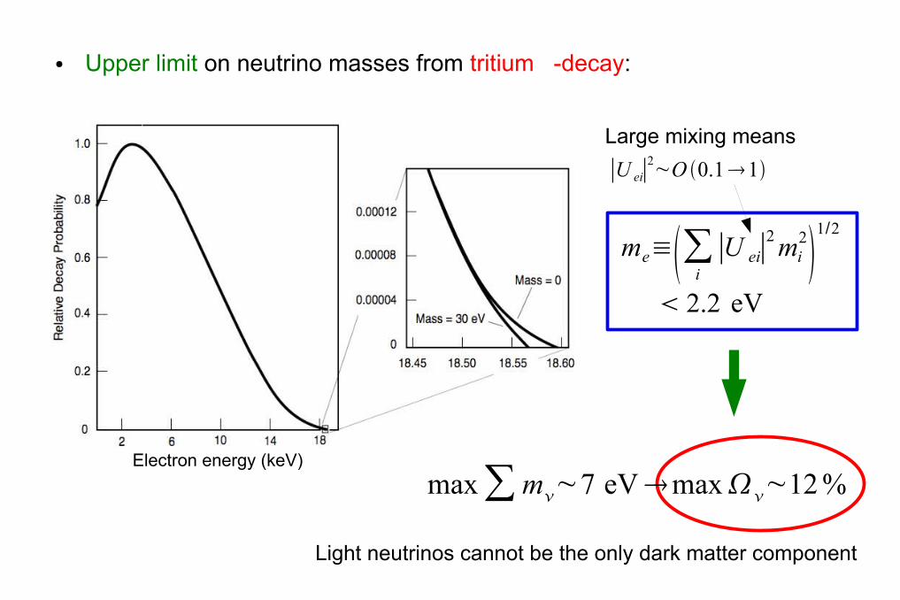
● Upper limit on neutrino masses from tritium � -decay:
Electron energy (keV)
me≡∑i ∣U ei∣2mi
21/2
2.2 eV
Large mixing means ∣U ei∣
2~O 0.11
Light neutrinos cannot be the only dark matter component
max∑m~7 eVmax~12%
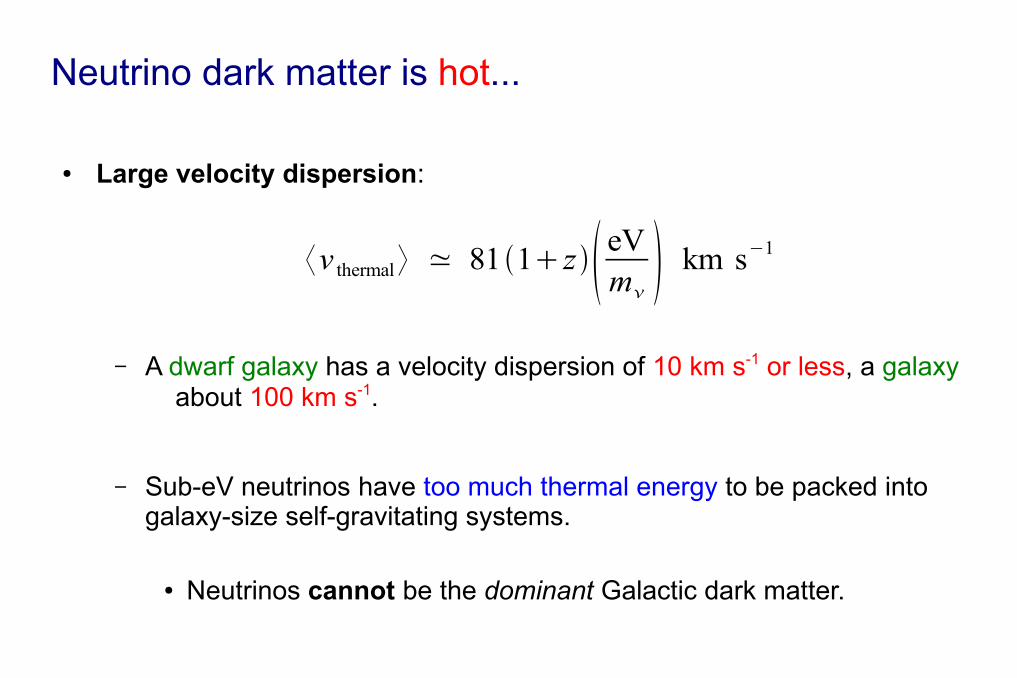
Neutrino dark matter is hot...
● Large velocity dispersion:
– A dwarf galaxy has a velocity dispersion of 10 km s-1 or less, a galaxy about 100 km s-1.
– Sub-eV neutrinos have too much thermal energy to be packed into galaxy-size self-gravitating systems.
● Neutrinos cannot be the dominant Galactic dark matter.
⟨v thermal⟩ ≃ 81 1z eVm km s−1
● Hot dark matter leaves a distinctive imprint on the large-scale structure distribution.
– We can learn about neutrino properties from cosmology.
● Cosmological probes are getting ever more precise:
– Even a small neutrino mass can bias the inference of other cosmological parameters.
Why study neutrinos in cosmology...

The concordance framework...
Baryons
● We work within the � CDM framework extended with a subdominant component of massive neutrino dark matter.
– Flat geometry.
– Main dark matter is cold.
– Initial conditions from single-field slow-roll inflation.

The concordance framework...
Baryons
?% Massiveneutrinos
● We work within the � CDM framework extended with a subdominant component of massive neutrino dark matter.
– Flat geometry.
– Main dark matter is cold.
– Initial conditions from single-field slow-roll inflation.

Plan...
● What we can do now
● What we can do in the future
● The nonlinear matter power spectrum

1. What we can do now...

● On the background:
– Shift in time of matter radiation equality.
● On the perturbations:
– Suppression of growth.
Two effects of massive neutrinos...

● Sub-eV neutrinos become nonrelativistic at z<1000:
– Radiation at early times.
– Matter at late times.
– Shift in matter-radiation equality relative to model with zero neutrino mass.
Background...
Comoving matter density today ≠ Comoving matter density before recombination
mν = 1 eVmν = 0 eV
● On the background:
– Shift in time of matter radiation equality.
● On the perturbations:
– Suppression of growth.
Two effects of massive neutrinos...

● At low redshifts, neutrinos become nonrelativistic:.
– But still have large thermal speed:
→ hinder � clustering on small scales.
● Free-streaming length scale & wavenumber:
Perturbations...
c
ν ν
c
FS≡ 82c2
3mH2≃4.2 1z
m,0 eVm h−1 Mpc
k FS≡2FS
c≃811z eVm km s−1
≫FS
k≪k FS
Clustering
≪FS
k≫k FSNon-clustering
Gravitationalpotential wells

● In turn, free-streaming (non-clustering) neutrinos slow down the growth of gravitational potential wells on scales λ << λFS or wavenumbers k >> kFS.
c
ν ν
c
c ν
ν
c
c cν ν c ν
Clustering → potential wells become deeper
Some time later...
Only CDM clusters
Both CDM andneutrinos cluster

● The presence of HDM slows down the growth of CDM perturbations at large wavenumbers k.
– The density perturbation spectrum acquires a step-like feature.
δcdm δcdm
CDM-only
CHDM
k k
Initial time... Some time later...
kFS

Describing perturbations: CDM...
● Cold dark matter = collisionless, pressureless fluid:
cc=0
cH c∇2=0
Continuity eqn
Euler eqn
Gravitational source
Poisson eqn ∇ 2= 32H 2m [ f cc f ]
Density perturbations
Velocity divergencef ≡
m
Neutrino fraction
Expansion

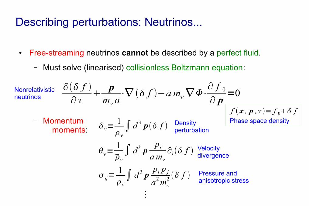
Describing perturbations: Neutrinos...
● Free-streaming neutrinos cannot be described by a perfect fluid.
– Must solve (linearised) collisionless Boltzmann equation:
f x , p ,= f 0 fPhase space density
Nonrelativisticneutrinos
∂ f ∂
pma
⋅∇ f −a m∇⋅∂ f 0
∂ p=0
Describing perturbations: Neutrinos...
● Free-streaming neutrinos cannot be described by a perfect fluid.
– Must solve (linearised) collisionless Boltzmann equation:
– Momentum moments:
f x , p ,= f 0 fPhase space density
Nonrelativisticneutrinos
∂ f ∂
pma
⋅∇ f −a m∇⋅∂ f 0
∂ p=0
≡1
∫d 3 p f
≡1
∫ d3 p
pia m
∂i f
ij≡1∫ d 3 p
pi p ja2m
2 f
⋮
Density perturbation
Velocitydivergence
Pressure and anisotropic stress
Give rise tofree-streamingbehaviour

δcdm δb δγδν
ψ, φ
~ a
Lesgourgues and Pastor 2006
kFS >>
Massive neutrinos, mν=1 eVk=10−2h Mpc−1≪k FS
Clustering regime

a1-3/5fνa
(fν = Ων/Ωm)
Lesgourgues and Pastor 2006
Massive neutrinos, mν=1 eV
kFS <<
k=1h Mpc−1≫k FS
Non-clustering regime
δcdmδb
δγ
δν
ψ, φ
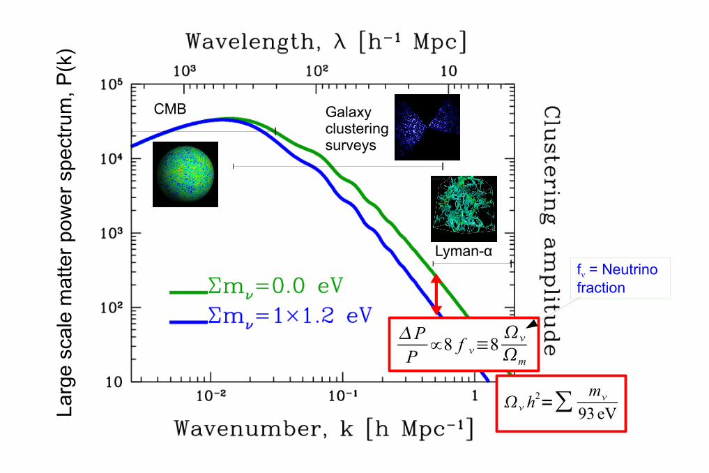
CMB Galaxy clustering surveys
Lyman-α
h2=∑ m
93 eV
fν = Neutrino fraction
PP∝8 f ≡8
m
Larg
e s
cale
mat
ter
pow
er
spe
ctru
m, P
(k)

CMB
Lyman-α
h2=∑ m
93 eV
fν = Neutrino fraction
Galaxy clustering surveys
PP∝8 f ≡8
m
Larg
e s
cale
mat
ter
pow
er
spe
ctru
m, P
(k)

CMB
Lyman-α
h2=∑ m
93 eV
fν = Neutrino fraction
Galaxy clustering surveys
PP∝8 f ≡8
m
Larg
e s
cale
mat
ter
pow
er
spe
ctru
m, P
(k)
“Linear”≡ k
3Pk 22
≪1
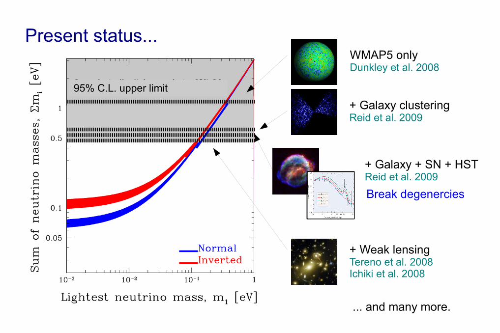
Present status...WMAP5 only Dunkley et al. 2008
+ Galaxy clusteringReid et al. 2009
+ Galaxy + SN + HSTReid et al. 2009
Break degenercies
... and many more.
95% C.L. upper limit
+ Weak lensingTereno et al. 2008 Ichiki et al. 2008

2. What we can do in the future...

Planck
SNAP
WFMOS
MWA
Photometric galaxy surveys with lensingcapacity, zmax~3
High-z spectroscopic galaxy surveys,z > 2
Radio arrays,5 < z < 15

● Weak lensing
– of galaxies
– of the CMB
● 21 cm emission
● ISW effect
● Cluster abundance
Possible new techniques...
Song & Knox 2004Hannestad, Tu & Y3W 2006Kitching et al. 2008
Lesgourgues et al. 2006Perotto, Lesgourgues, Hannestad, Tu & Y3W, 2006
Mao et al. 2008Pritchard & Pierpaoli 2008Metcalf 2009
Ichikawa & Takahashi 2005Lesgourgues, Valkenburg & Gaztañaga 2007
Wang et al. 2005
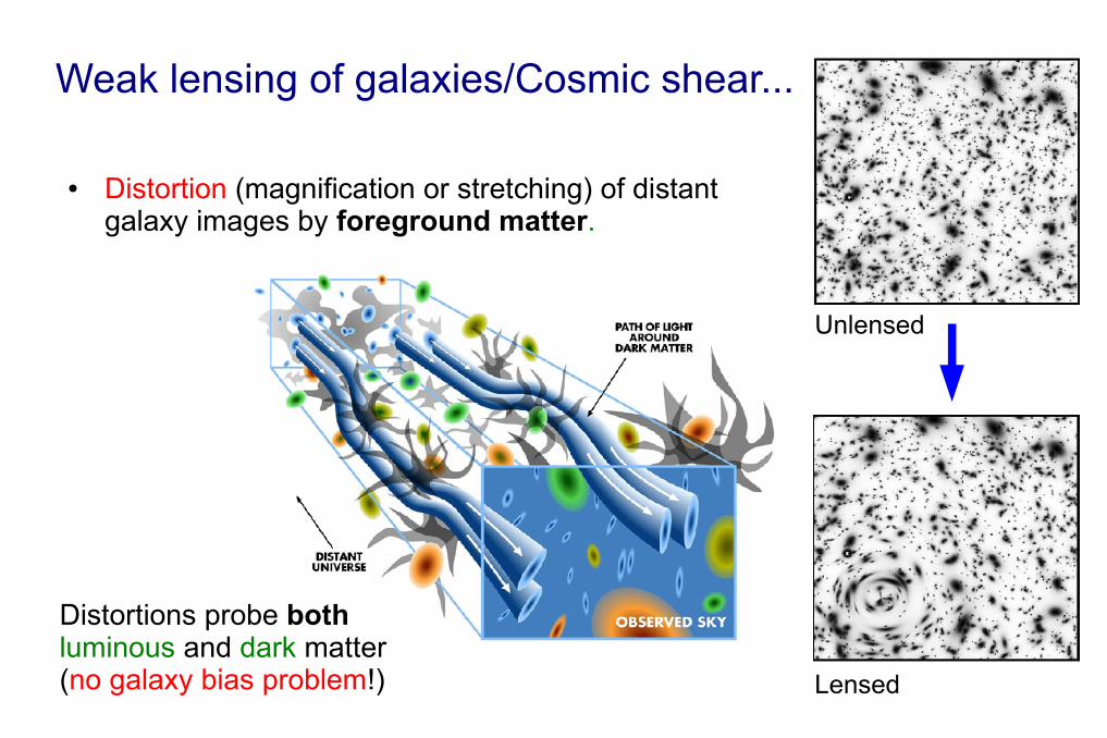
● Distortion (magnification or stretching) of distant galaxy images by foreground matter.
Unlensed
Lensed
Weak lensing of galaxies/Cosmic shear...
Distortions probe both luminous and dark matter(no galaxy bias problem!)

Galaxies are randomly oriented, i.e., no “preferred direction”.
Lensing leads to a “preferred direction”.
“Average” galaxy shapes over cell
Lensed
Unlensed

Shear map
Weak lensing theory predicts:
Cluster
Void
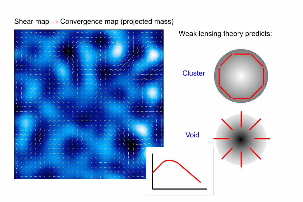
Cluster
Void
Shear map → Convergence map (projected mass)
Weak lensing theory predicts:

● Tomography = bin galaxy images by redshift
z
Tomography probes spectrum evolution and the growth function.
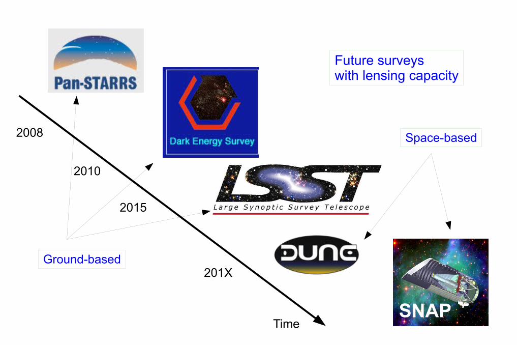
SNAP
Time
Future surveyswith lensing capacity
2008
2010
2015
201XGround-based
Space-based
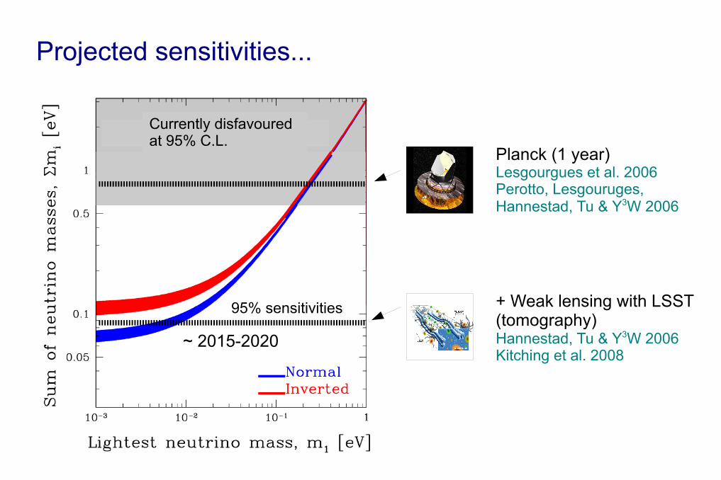
Currently disfavoured at 95% C.L.
Projected sensitivities...
+ Weak lensing with LSST(tomography)Hannestad, Tu & Y3W 2006Kitching et al. 2008
Planck (1 year)Lesgourgues et al. 2006Perotto, Lesgouruges, Hannestad, Tu & Y3W 2006
95% sensitivities
~ 2015-2020
95% sensitivities95% sensitivities95% sensitivities95% sensitivities
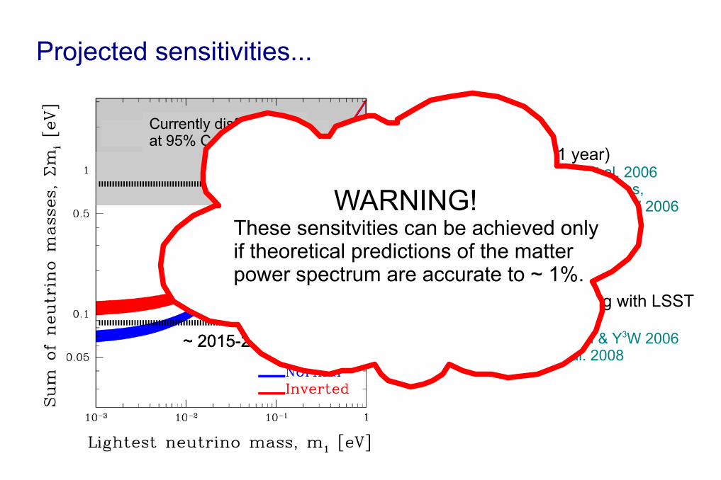
Currently disfavoured at 95% C.L.
Projected sensitivities...
+ Weak lensing with LSST(tomography)Hannestad, Tu & Y3W 2006Kitching et al. 2008
Planck (1 year)Lesgourgues et al. 2006Perotto, Lesgouruges, Hannestad, Tu & Y3W 2006
~ 2015-2020
Currently disfavoured at 95% C.L.
~ 2015-2020
WARNING!These sensitvities can be achieved onlyif theoretical predictions of the matter power spectrum are accurate to ~ 1%.

3. The nonlinear matter power spectrum...

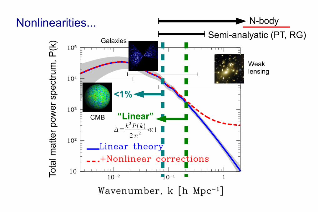
Nonlinearities...
<1%
“Linear”
N-body
CMB
Galaxies
Weaklensing
≡ k3Pk 22
≪1
Semi-analyatic (PT, RG)
Tota
l mat
ter
pow
er s
pec
tru
m, P
(k)
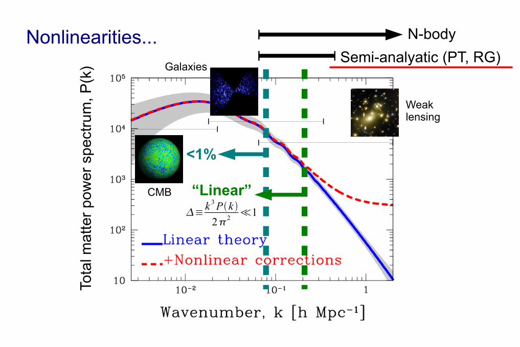
Nonlinearities...
<1%
“Linear”
N-body
CMB
Galaxies
Weaklensing
≡ k3Pk 22
≪1
Semi-analyatic (PT, RG)
Tota
l mat
ter
pow
er s
pec
tru
m, P
(k)

z = 4
z = 0
512 h-1 Mpc
Brandbyge, Hannestad, Haugbølle & Thomsen 2008Brandbyge and Hannestad 2008, 2009
N-body simulations with massive neutrinos...
● Particle representation for both CDM and neutrinos.
– Modified GADGET-2.
– Neutrino particles drawn from Fermi-Dirac distribution.
CDM density � density ∑mν=0.6 eV
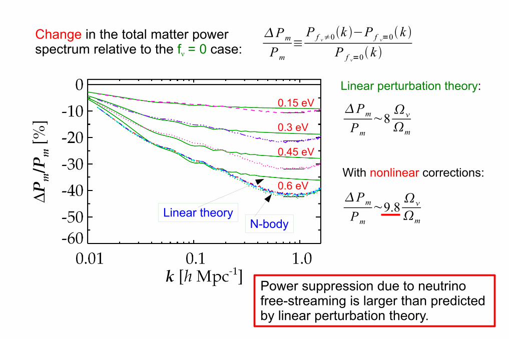
PmPm
~8
m
PmPm
~9.8
m
Linear perturbation theory:
With nonlinear corrections:
Power suppression due to neutrino free-streaming is larger than predicted by linear perturbation theory.
N-body
PmPm
≡P f ≠0k −P f =0k
P f =0k Change in the total matter power spectrum relative to the fν = 0 case:
Linear theory
0.6 eV
0.15 eV
0.3 eV
0.45 eV
Nonlinearities...
<1%
“Linear”
N-body
CMB
Galaxies
Weaklensing
≡ k3Pk 22
≪1
Semi-analyatic (PT, RG)
Tota
l mat
ter
pow
er s
pec
tru
m, P
(k)
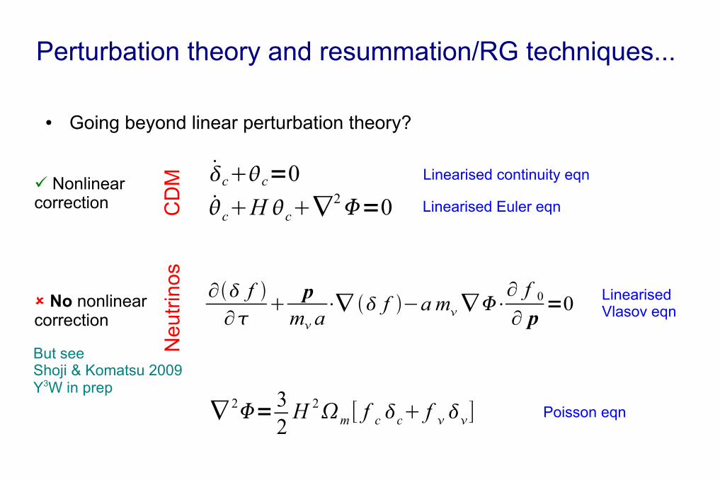
Perturbation theory and resummation/RG techniques...
● Going beyond linear perturbation theory?
cc=0
cH c∇2=0
Linearised continuity eqn
Linearised Euler eqn
∂ f ∂
pma
⋅∇ f −a m∇⋅∂ f 0
∂ p=0
Poisson eqn∇ 2= 32H 2m [ f cc f ]
CD
MN
eutr
inos
LinearisedVlasov eqn
Nonlinear correction
No nonlinear correction
But seeShoji & Komatsu 2009Y3W in prep

c k ,H ck ,−k2k ,=
ck ,c k ,=Continuity eqn
Euler eqn
● Fluid description (linear):
δc = CDM density perturbationsδν = ν density perturbationsθc = Divergence of velocity field
k 2=− 32H 2m[ f cc f ]
Poisson eqn
Corrections to the CDM component...
0
0

c k ,H ck ,−k2k ,=
222 k ,q1 ,q2≡Dk−q12q12
2 q1⋅q2
2q12q2
2
−∫ d 3q1d3q2121 k ,q1 ,q2 c q1 ,cq2 ,ck ,c k ,=
−∫ d 3q1d3q2222 k ,q1 ,q2cq1 ,cq2 ,
Continuity eqn
Euler eqn
Vertex● Fluid description (incl. some nonlinear terms):121 k ,q1 ,q2≡D k−q12
q12⋅q1
q12
Vertex
δc = CDM density perturbationsδν = ν density perturbationsθc = Divergence of velocity field
Mode coupling
k 2=− 32H 2m[ f cc f ]
Poisson eqn
Starting point of most semi-analytic calculations in the literature.
Corrections to the CDM component...
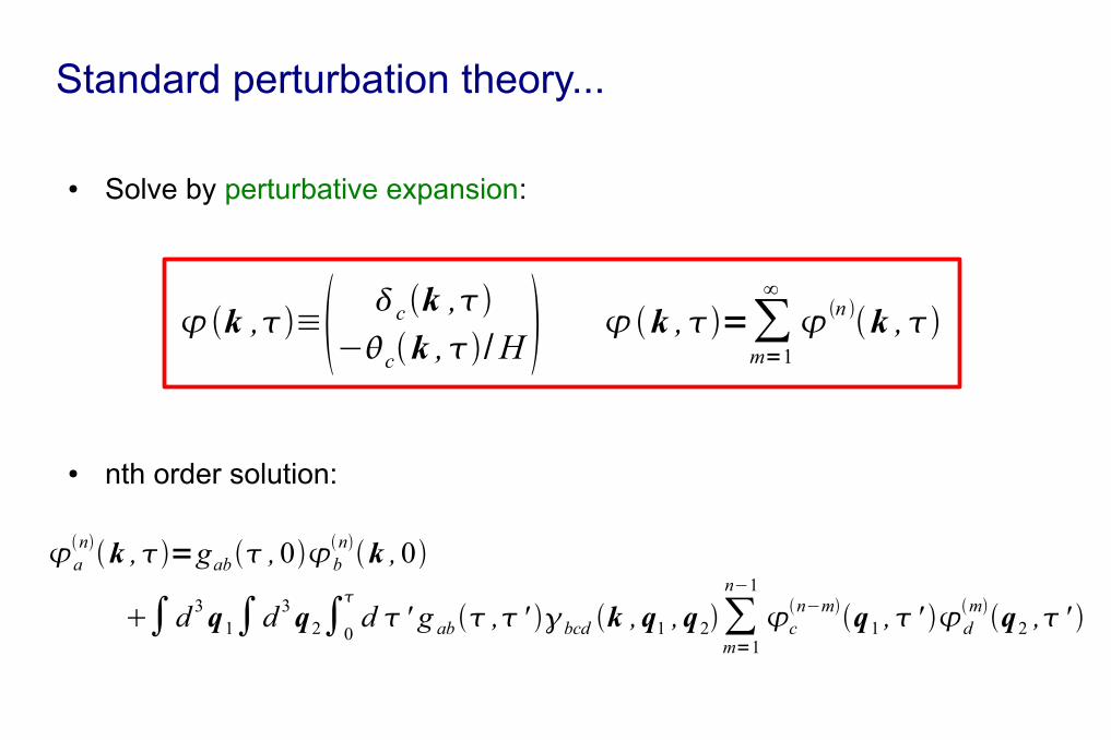
● Solve by perturbative expansion:
● nth order solution:
Standard perturbation theory...
k ,≡ c k ,−ck ,/H k ,=∑
m=1
∞
n k ,
ank ,=gab ,0b
nk ,0
∫d 3q1∫d 3q2∫0
d ' g ab , ' bcd k ,q1 ,q2∑
m=1
n−1
cn−mq1 , ' d
mq2 , '

Density/Velocity
= + ...
k =1 23...
++
Crocce & Scoccimarro 2006Matarrese & Pietroni 2007
gab ,0
b10a
1q1
q2
'
time

= + ...
k =1 23...
++
Crocce & Scoccimarro 2006Matarrese & Pietroni 2007
gab ,0
b10a
1q1
q2
'
Pk Dkk ' ≡⟨k k ' ⟩=⟨11⟩[⟨22⟩2 ⟨13⟩ ]...
Power spectrum
= + ...+ + 2
“One-loop” correctionLinear
“22” “13”“11”
Density/Velocity
time
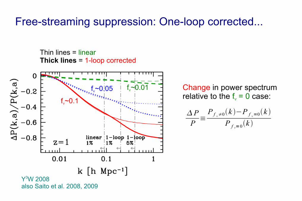
Free-streaming suppression: One-loop corrected...
fν~0.1
fν~0.05 fν~0.01
Thin lines = linearThick lines = 1-loop corrected
PP≡P f ≠0k −P f =0k
P f =0k
Change in power spectrumrelative to the fν = 0 case:
Y3W 2008also Saito et al. 2008, 2009

Free-streaming suppression: One-loop corrected...
fν~0.1
fν~0.05 fν~0.01
Thin lines = linearThick lines = 1-loop corrected
N-body simulations, Brandbyge et al. 2008
Y3W 2008also Saito et al. 2008, 2009
● Many schemes have been proposed that go beyond standard perturbation theory:
Crocce & Scoccimarro 2006, 2008
Taruya & Hiramatsu 2007
McDonald 2007
Matarresse & Pietroni 2007, 2008
Matsubara 2008
Valageas 2007
Pietroni 2008
Hiramatsu & Taruya 2009
etc..
Resummation and renormalisation group techniques...

● Applied to massive neutrino cosmologies:
Lesgourgues, Matarrese, Pietroni & Riotto 2009
P(m
�)/P
(m�=
0)
k (h/Mpc)0.5
= One-loop= Time-RG flow= N-body= Linear
z = 4
z = 1 z = 0
z= 2.33
0.0 0.50.0
1.00.01.00.0 1.00.0
0.5
0.9
0.8
0.6
0.5
0.7
0.9
0.8
0.6
0.5
0.7
0.9
0.8
0.6
0.5
0.7
∑mν = 0.3 eV
∑mν = 0.6 eV
0.9
0.8
0.6
0.5
0.7

Summary...
● Using the large-scale structure distribution to probe neutrino physics is still fun.
– We can do even better in the future with forthcoming probes/new techniques.
● But we must make sure our theoretical predictions are reliable (1% accurate) at the (nonlinear) scales of interest.
– N-body simulations are the definitive way to go.
– Semi-analytic PT & RG techniques are also of some (limited) use.