arX

iv:h

ep-p

h/03

1023

8v2

1 O

ct 2

004

hep-ph/0310238

Neutrino MixingCarlo Giunti

INFN, Sezione di Torino, and Dipartimento di Fisica Teorica,Universita di Torino, Via P. Giuria 1, I–10125 Torino, Italy

Marco Laveder

Dipartimento di Fisica “G. Galilei”, Universita di Padova,and INFN, Sezione di Padova, Via F. Marzolo 8, I–35131 Padova, Italy

Abstract

In this review we present the main features of the current status ofneutrino physics. After a review of the theory of neutrino mixing andoscillations, we discuss the current status of solar and atmospheric neu-trino oscillation experiments. We show that the current data can benicely accommodated in the framework of three-neutrino mixing. Wediscuss also the problem of the determination of the absolute neutrinomass scale through Tritium β-decay experiments and astrophysical ob-servations, and the exploration of the Majorana nature of massive neu-trinos through neutrinoless double-β decay experiments. Finally, futureprospects are briefly discussed.

PACS Numbers: 14.60.Pq, 14.60.Lm, 26.65.+t, 96.40.TvKeywords: Neutrino Mass, Neutrino Mixing, Solar Neutrinos, Atmospheric Neutrinos

1

Contents

Contents 2

1 Introduction 3

2 Neutrino masses and mixing 32.1 Dirac mass term . . . . . . . . . . . . . . . . . . . . . . . . . . . . . . . . 42.2 Majorana mass term . . . . . . . . . . . . . . . . . . . . . . . . . . . . . 42.3 Dirac-Majorana mass term . . . . . . . . . . . . . . . . . . . . . . . . . . 52.4 The see-saw mechanism . . . . . . . . . . . . . . . . . . . . . . . . . . . 72.5 Effective dimension-five operator . . . . . . . . . . . . . . . . . . . . . . 82.6 Three-neutrino mixing . . . . . . . . . . . . . . . . . . . . . . . . . . . . 9

3 Theory of neutrino oscillations 133.1 Neutrino oscillations in vacuum . . . . . . . . . . . . . . . . . . . . . . . 133.2 Neutrino oscillations in matter . . . . . . . . . . . . . . . . . . . . . . . . 17

4 Neutrino oscillation experiments 254.1 Solar neutrino experiments and KamLAND . . . . . . . . . . . . . . . . 264.2 Atmospheric neutrino experiments and K2K . . . . . . . . . . . . . . . . 304.3 The reactor experiment CHOOZ . . . . . . . . . . . . . . . . . . . . . . . 33

5 Phenomenology of three-neutrino mixing 345.1 Three-neutrino mixing schemes . . . . . . . . . . . . . . . . . . . . . . . 355.2 Tritium β-decay . . . . . . . . . . . . . . . . . . . . . . . . . . . . . . . . 385.3 Cosmological bounds on neutrino masses . . . . . . . . . . . . . . . . . . 395.4 Neutrinoless double-β decay . . . . . . . . . . . . . . . . . . . . . . . . . 41

6 Future prospects 42

7 Conclusions 44

References 44

2

1 Introduction

The last five years have seen enormous progress in our knowledge of neutrino physics.We have now strong experimental evidences of the existence of neutrino oscillations,predicted by Pontecorvo in the late 50’s [1, 2], which occur if neutrinos are massive andmixed particles.

In 1998 the Super-Kamiokande experiment [3] provided a model-independent proofof the oscillations of atmospheric muon neutrinos, which were discovered in 1988 by theKamiokande [4] and IMB [5] experiments. The values of the neutrino mixing parametersthat generate atmospheric neutrino oscillations have been confirmed at the end of 2002by the first results of the K2K long-baseline accelerator experiment [6], which observeda disappearance of muon neutrinos due to oscillations.

In 2001 the combined results of the SNO [7] and Super-Kamiokande [8] experimentsgave a model-independent indication of the oscillations of solar electron neutrinos, whichwere discovered in the late 60’s by the Homestake experiment [9]. In 2002 the SNOexperiment [10] measured the total flux of active neutrinos from the sun, providing amodel-independent evidence of oscillations of electron neutrinos into other flavors, whichhas been confirmed with higher precision by recent data [11]. The values of the neutrinomixing parameters indicated by solar neutrino data have been confirmed at the end of2002 by the KamLAND very-long-baseline reactor experiment [12], which have measureda disappearance of electron antineutrinos due to oscillations.

In this paper we review the currently favored scenario of three-neutrino mixing, whichis based on the above mentioned evidences of neutrino oscillations. In Section 2 we reviewthe theory of neutrino masses and mixing, showing that it is likely that massive neutrinosare Majorana particles. In Section 3 we review the theory of neutrino oscillations invacuum and in matter. In Section 4 we review the main results of neutrino oscillationexperiments. In Section 5 we discuss the main aspects of the phenomenology of three-neutrino mixing, including neutrino oscillations, experiments on the measurement of theabsolute scale of neutrino masses and neutrinoless double-β decay experiments searchingfor an evidence of the Majorana nature of massive neutrinos. In Section 6 we discusssome future prospects and in Section 7 we draw our conclusions.

For further information on the physics of massive neutrinos, see the books in Refs. [13,14, 15], the reviews in Refs. [16, 17, 18, 19, 20, 21, 22, 23, 24, 25, 26, 27, 26, 28, 29, 30,31, 32, 33, 34, 35, 36, 37, 38] and the references in Ref. [39].

2 Neutrino masses and mixing

The Standard Model was formulated in the 60’s [40, 41, 42] on the basis of the knowledgeavailable at that time on the existing elementary particles and their properties. In partic-ular, neutrinos were though to be massless following the so-called two-component theoryof Landau [43], Lee and Yang [44], and Salam [45], in which the massless neutrinos aredescribed by left-handed Weyl spinors. This description has been reproduced in the Stan-dard Model of Glashow [40], Weinberg [41] and Salam [42] assuming the non existenceof right-handed neutrino fields, which are necessary in order to generate Dirac neutrinomasses with the same Higgs mechanism that generates the Dirac masses of quarks andcharged leptons. However, as will be discussed in Section 4, in recent years neutrino

3

experiments have shown convincing evidences of the existence of neutrino oscillations,which is a consequence of neutrino masses and mixing. Hence, it is time to revise theStandard Model in order to take into account neutrino masses (notice that the StandardModel has already been revised in the early 70’s with the inclusion first of the charmedquark and after of the third generation).

2.1 Dirac mass term

Considering for simplicity only one neutrino field ν, the standard Higgs mechanism gen-erates the Dirac mass term

LD = −mD ν ν = −mD (νR νL + νL νR) , (2.1)

with mD = y v/√

2 where y is a dimensionless Yukawa coupling coefficient and v/√

2 isthe Vacuum Expectation Value of the Higgs field. νL and νR are, respectively, the chiralleft-handed and right-handed components of the neutrino field, obtained by acting on νwith the corresponding projection operator:

ν = νL + νR , νL = PL ν , νR = PR ν , PL ≡ 1 − γ5

2, PR ≡ 1 + γ5

2, (2.2)

such that PLPR = PRPL = 0, P 2L = PL, P 2

R = PR, since (γ5)2 = 1. Therefore, we have

PL νL = νL , PL νR = 0 , PR νL = 0 , PR νR = νR . (2.3)

It can be shown that the chiral spinors νL and νR have only two independent componentseach, leading to the correct number of four for the independent components of the spinorν.

Unfortunately, the generation of Dirac neutrino masses through the standard Higgsmechanism is not able to explain naturally why the neutrino are more than five orderof magnitude lighter than the electron, which is the lightest of the other elementaryparticles (as discussed in Section 4, the neutrino masses are experimentally constrainedbelow about 1-2 eV). In other words, there is no explanation of why the neutrino Yukawacoupling coefficients are more than five order of magnitude smaller than the Yukawacoupling coefficients of quarks and charged leptons.

2.2 Majorana mass term

In 1937 Majorana [46] discovered that a massive neutral fermion as a neutrino can bedescribed by a spinor ψ with only two independent components imposing the so-calledMajorana condition

ψ = ψc , (2.4)

where ψc = CψT= Cγ0T

ψ∗ is the operation of charge conjugation, with the charge-conjugation matrix C defined by the relations CγµTC−1 = −γµ, C† = C−1, CT = −C.Since Cγ5TC−1 = γ5 and γ5γµ + γµγ5 = 0, we have

PL ψcL = 0 , PL ψ

cR = ψc

R , PR ψcL = ψc

L , PR ψcR = 0 . (2.5)

4

In other words, ψcL is right-handed and ψc

R is left-handed.Decomposing the Majorana condition (2.4) into left-handed and right-handed com-

ponents, ψL + ψR = ψcL + ψc

R, and acting on both members of the equation with theright-handed projector operator PR, we obtain

ψR = ψcL . (2.6)

Thus, the right-handed component ψR of the Majorana neutrino field ψ is not indepen-dent, but obtained from the left-handed component ψL through charge conjugation andthe Majorana field can be written as

ψ = ψL + ψcL . (2.7)

This field depends only on the two independent components of ψL. Using the constraint(2.6) in the mass term (2.1), we obtain the Majorana mass term

LM = −1

2mM

(ψc

L ψL + ψL ψcL

), (2.8)

where we have inserted a factor 1/2 in order to avoid double counting in the Euler-Lagrange derivation of the equation for the Majorana neutrino field.

2.3 Dirac-Majorana mass term

In general, if both the chiral left-handed and right-handed fields exist and are indepen-dent, in addition to the Dirac mass term (2.1) also the Majorana mass terms for νL andνR are allowed:

LML = −1

2mL

(νc

L νL + νL νcL

), LM

R = −1

2mR

(νc

R νR + νR νcR

). (2.9)

The total Dirac+Majorana mass term

LD+M = LD + LML + LM

R (2.10)

can be written as

LD+M = −1

2

(νc

L νR

)(mL mD

mD mR

)(νL

νcR

)+ H.c. . (2.11)

It is clear that the chiral fields νL and νR do not have a definite mass, since they arecoupled by the Dirac mass term. In order to find the fields with definite masses it isnecessary to diagonalize the mass matrix in Eq. (2.11). For this task, it is convenient towrite the Dirac+Majorana mass term in the matrix form

LD+M =1

2N c

LM NL + H.c. , (2.12)

with the matrices

M =

(mL mD

mD mR

), NL =

(νL

νcR

). (2.13)

5

The column matrix NL is left-handed, because it contains left-handed fields. Let us writeit as

NL = U nL , with nL =

(ν1L

ν2L

), (2.14)

where U is the unitary mixing matrix (U † = U−1) and nL is the column matrix of theleft-handed components of the massive neutrino fields. The Dirac+Majorana mass termis diagonalized requiring that

UT M U =

(m1 00 m2

), (2.15)

with mk real and positive for k = 1, 2.Let us consider the simplest case of a real mass matrix M . Since the values of mL

and mR can be chosen real and positive by an appropriate choice of phase of the chiralfields νL and νR, the mass matrix M is real if mD is real. In this case, the mixing matrixU can be written as

U = O ρ , (2.16)

where O is an orthogonal matrix and ρ is a diagonal matrix of phases:

O =

(cosϑ sinϑ− sinϑ cosϑ

), ρ =

(ρ1 00 ρ2

), (2.17)

with |ρk|2 = 1. The orthogonal matrix O is chosen in order to have

OT M O =

(m′

1 00 m′

2

), (2.18)

leading to

tan 2ϑ =2mD

mR −mL, m′

2,1 =1

2

[mL +mR ±

√(mL −mR)2 + 4m2

D

]. (2.19)

Having chosen mL and mR positive, m′2 is always positive, but m′

1 is negative if m2D >

mLmR. Since

UT M U = ρT OT M O ρ =

(ρ2

1m′1 0

0 ρ22m

′2

), (2.20)

it is clear that the role of the phases ρk is to make the masses mk positive, as massesmust be. Hence, we have ρ2

2 = 1 always, and ρ21 = 1 if m′

1 ≥ 0 or ρ21 = −1 if m′

1 < 0.An important fact to be noticed is that the diagonalized Dirac+Majorana mass term,

LD+M =1

2

∑

k=1,2

mk νckL νkL + H.c. , (2.21)

is a sum of Majorana mass terms for the massive Majorana neutrino fields

νk = νkL + νckL (k = 1, 2) . (2.22)

Therefore, the two massive neutrinos are Majorana particles.

6

2.4 The see-saw mechanism

It is possible to show that the Dirac+Majorana mass term leads to maximal mixing(θ = π/4) if mL = mR, or to so-called pseudo-Dirac neutrinos if mL and mR are muchsmaller that |mD| (see Ref. [21]). However, the most plausible and interesting case isthe so-called see-saw mechanism [47, 48, 49], which is obtained considering mL = 0 and|mD| ≪ mR. In this case

m1 ≃(mD)2

mR

≪ |mD| , m2 ≃ mR , tanϑ ≃ mD

mR

≪ 1 , ρ21 = −1 . (2.23)

What is interesting in Eq. (2.23) is that m1 is much smaller than mD, being suppressedby the small ratio mD/mR. Since m2 is of order mR, a very heavy ν2 corresponds to avery light ν1, as in a see-saw. Since mD is a Dirac mass, presumably generated with thestandard Higgs mechanism, its value is expected to be of the same order as the mass of aquark or the charged fermion in the same generation of the neutrino we are considering.Hence, the see-saw explains naturally the suppression of m1 with respect to mD, providingthe most plausible explanation of the smallness of neutrino masses.

The smallness of the mixing angle ϑ in Eq. (2.23) implies that ν1L ≃ −νL and ν2L ≃ νcR.

This means that the neutrino participating to weak interactions practically coincideswith the light neutrino ν1, whereas the heavy neutrino ν2 is practically decoupled frominteractions with matter.

Besides the smallness of the light neutrino mass, another important consequence of thesee-saw mechanism is that massive neutrinos are Majorana particles, as we have shownabove in the general case of a Dirac+Majorana mass term. This is a very importantindication that strongly encourages the search for the Majorana nature of neutrinos,mainly performed through the search of neutrinoless double-β decay.

An important assumption necessary for the see-saw mechanism is mL = 0. Suchassumption may seem arbitrary at first sight, but in fact it is not. Its plausibility followsfrom the fact that νL belongs to a weak isodoublet of the Standard Model:

LL =

(νL

ℓL

). (2.24)

Since νL has third component of the weak isospin I3 = 1/2, the combination νcLνL =

−νTLC†νL in the Majorana mass term in Eq. (2.9) has I3 = 1 and belongs to a triplet. Since

in the Standard Model there is no Higgs triplet that could couple to νcLνL in order to form

a Lagrangian term invariant under a SU(2)L transformation of the Standard Model gaugegroup, a Majorana mass term for νL is forbidden. In other words, the gauge symmetriesof the Standard Model imply mL = 0, as needed for the see-saw mechanism. On theother hand, mD is allowed in the Standard Model, because it is generated through thestandard Higgs mechanism, and mR is also allowed, because νR and νc

RνR are singlets ofthe Standard Model gauge symmetries. Hence, quite unexpectedly, we have an extendedStandard Model with massive neutrinos that are Majorana particles and in which thesmallness of neutrino masses can be naturally explained through the see-saw mechanism.

The only assumption which remains unexplained in this scenario is the heaviness ofmR with respect to mD. This assumption cannot be motivated in the framework of theStandard Model, because mR is only a parameter which could have any value. However,

7

there are rather strong arguments that lead us to believe that the Standard Model is atheory that describes the world only at low energies. In this case it is natural to expectthat the mass mR is generated at ultra-high energy by the symmetry breaking of thetheory beyond the Standard Model. Hence, it is plausible that the value of mR is manyorders of magnitude larger than the scale of the electroweak symmetry breaking and ofmD, as required for the working of the see-saw mechanism.

2.5 Effective dimension-five operator

If we consider the possibility of a theory beyond the Standard Model, another questionregarding the neutrino masses arises: is it possible that a Lagrangian term exists at thehigh energy of the theory beyond the Standard Model which generates at low energy aneffective Majorana mass term for νL? The answer is yes [50, 51, 52]: the operator withlowest dimension invariant1 under SU(2)L × U(1)Y that can generate a Majorana massterm for νL after electroweak symmetry breaking is the dimension-five operator2

g

M(LTL σ2 Φ) C−1 (ΦT σ2 LL) + H.c. , (2.25)

where g is a dimensionless coupling coefficient and M is the high-energy scale at whichthe new theory breaks down to the Standard Model. The dimension-five operator inEq. (2.25) does not belong to the Standard Model because it is not renormalizable. Itmust be considered as an effective operator which is the low-energy manifestation of therenormalizable new theory beyond the Standard Model, in analogy with the old non-renormalizable Fermi theory of weak interactions, which is the low-energy manifestationof the Standard Model.

At the electroweak symmetry breaking

Φ =

(φ+

φ0

)Symmetry Breaking−−−−−−−−−−−→

(0

v/√

2

), (2.26)

the operator in Eq. (2.25) generates the Majorana mass term for νL in Eq. (2.9), with

mL =g v2

M . (2.27)

This relation is very important, because it shows that the Majorana massmL is suppressedwith respect to v by the small ratio v/M. In other words, since the Dirac mass term mD

is equal to v/√

2 times a Yukawa coupling coefficient, the relation (2.27) has a see-sawform. Therefore, the effect of the dimension-five effective operator in Eq. (2.25) doesnot spoil the natural suppression of the light neutrino mass provided by the see-saw

1Since the high-energy theory reduces to the Standard Model at low energies, its gauge symmetriesmust include the gauge symmetries of the Standard Model.

2In units where ~ = c = 1 scalar fields have dimension of energy, fermion fields have dimen-sion of (energy)3/2 and all Lagrangian terms have dimension (energy)4. The “dimension-five” char-acter of the operator in Eq. (2.25) refers to the power of energy of the dimension of the operator(LT

L σ2 Φ) C−1 (ΦT σ2 LL), which is divided by the mass M in order to obtain a Lagrangian term withcorrect dimension.

8

mechanism. Indeed, considering mL ∼ m2D/mR and taking into account that m1 = |m′

1|,from Eq. (2.19) we obtain

m1 ≃∣∣∣∣mL − (mD)2

mR

∣∣∣∣ . (2.28)

Equations (2.27) and (2.28) show that the see-saw mechanism is operating even if mL isnot zero, but it is generated by the dimension-five operator in Eq. (2.25). On the otherhand, if the chiral right-handed neutrino field νR does not exist, the standard see-sawmechanism cannot be implemented, but a Majorana neutrino mass mL can be generatedby the dimension-five operator in Eq. (2.25), and Eq. (2.27) shows that the suppressionof the light neutrino mass is natural and of see-saw type.

2.6 Three-neutrino mixing

So far we have considered for simplicity only one neutrino, but it is well known froma large variety of experimental data that there are three neutrinos that participate toweak interactions: νe, νµ, ντ . These neutrinos are called “active flavor neutrinos”. Fromthe precise measurement of the invisible width of the Z-boson produced by the decays

Z →∑

α

νανα we also know that the number of active flavor neutrinos is exactly three

(see Ref. [53]), excluding the possibility of existence of additional heavy active flavorneutrinos3. The active flavor neutrinos take part in the charged-current (CC) and neutralcurrent (NC) weak interaction Lagrangians

LCCI = − g

2√

2jCCρ W ρ + H.c. , with jCC

ρ = 2∑

α=e,µ,τ

ναL γρ αL , (2.29)

LNCI = − g

2 cosϑWjNCρ Zρ , with jNC

ρ =∑

α=e,µ,τ

ναL γρ ναL , (2.30)

where jCCρ and jNC

ρ are, respectively, the charged and neutral leptonic currents, ϑW is theweak mixing angle (sin2 ϑW ≃ 0.23) and g = e/ sinϑW (e is the positron electric charge).

Let us consider three left-handed chiral fields νeL, νµL, ντL that describe the threeactive flavor neutrinos and three corresponding right-handed chiral fields νs1R, νs2R, νs3R

that describe three sterile neutrinos4, which do not take part in weak interactions. Thecorresponding Dirac+Majorana mass term is given by Eq. (2.10) with

LD = −∑

s,β

νsRMDsβ νβL + H.c. , (2.31)

LML = −1

2

∑

α,β

νcαL M

Lαβ νβL + H.c. , (2.32)

LMR = −1

2

∑

s,s′

νcsRM

Rαβ νs′R + H.c. , (2.33)

3More precisely, what is excluded is the existence of additional active flavor neutrinos with mass. mZ/2 ≃ 46 GeV [54]. For a recent discussion of the possible existence of heavier active flavor neutrinossee Ref. [55].

4Let us remark, however, that the number of sterile neutrinos is not constrained by experimentaldata, because they cannot be detected, and could well be different from three.

9

where MD is a complex matrix and ML, MR are symmetric complex matrices. TheDirac+Majorana mass term can be written as the one in Eq. (2.12) with the columnmatrix of left-handed fields

NL =

(νL

νcR

), with νL =

νeL

νµL

ντL

and νcR =

νc

s1R

νcs2R

νcs3R

, (2.34)

and the 6 × 6 mass matrix

M =

(ML (MD)T

MD MR

). (2.35)

The mass matrix is diagonalized by a unitary transformation analogous to the one inEq. (2.14):

NL = VnL , with nL =

ν1L...ν6L

, (2.36)

where V is the unitary 6 × 6 mixing matrix and nkL are the left-handed components ofthe massive neutrino fields. The mixing matrix V is determined by the diagonalizationrelation

VT M V = diag(m1, . . . , m6) , (2.37)

with mk real and positive for k = 1, . . . , 6 (see Ref. [17] for a proof that it can be done).After diagonalization the Dirac+Majorana mass term is written as

LD+M = −1

2

6∑

k=1

mk νckL νkL + H.c. , (2.38)

which is a sum of Majorana mass terms for the massive Majorana neutrino fields

νk = νkL + νckL (k = 1, . . . , 6) . (2.39)

Hence, as we have already seen in Section 2.3 in the case of one neutrino generation, aDirac+Majorana mass term implies that massive neutrinos are Majorana particles. Themixing relation (2.36) can be written as

ναL =6∑

k=1

Vαk νkL (α = e, µ, τ) , νcsR =

6∑

k=1

Vsk νkL (s = s1, s2, s3) , (2.40)

which shows that active and sterile neutrinos are linear combinations of the same massiveneutrino fields. This means that in general active-sterile oscillations are possible (seeSection 3).

The most interesting possibility offered by the Dirac+Majorana mass term is theimplementation of the see-saw mechanism for the explanation of the smallness of thelight neutrino masses, which is however considerably more complicated than in the caseof one generation discussed in Section 2.4. Let us assume that ML = 0, in compliance

10

with the gauge symmetries of the Standard Model and the absence of a Higgs triplet5.Let us further assume that the eigenvalues of MR are much larger than those of MD, asexpected if the Majorana mass term (2.33) for the sterile neutrinos is generated at a veryhigh energy scale characteristic of the theory beyond the Standard Model. In this case,we can write the mixing matrix V as

V = W U , (2.41)

where both W and U are unitary matrices, and use W for an approximate block-diagonalizationof the mass matrix M at leading order in the expansion in powers of (MR)−1MD:

WT M W ≃

(Mlight 0

0 Mheavy

). (2.42)

The matrix W is given by

W = 1 − 1

2

((MD)†(MR(MR)

†)−1MD 2(MD)†(MR)†

−1

−2(MR)−1MD (MR)−1MD(MD)†(MR)†−1

)

, (2.43)

and is unitary up to corrections of order (MR)−1MD. The two 3×3 mass matrices Mlight

and Mheavy are given by

Mlight ≃ −(MD)T (MR)−1MD , Mheavy ≃MR . (2.44)

Therefore, the see-saw mechanism is implemented by the suppression of Mlight with re-spect to MD by the small ratio (MD)T (MR)−1. The light and heavy mass sectors arepractically decoupled because of the smallness of the off-diagonal 3× 3 block elements inEq. (2.43).

For the low-energy phenomenology it is sufficient to consider only the light 3×3 massmatrix Mlight which is diagonalized by the 3 × 3 upper-left submatrix of U that we callU , such that

UT Mlight U = diag(m1, m2, m3) , (2.45)

where m1, m2, m3 are the three light neutrino mass eigenvalues. Neglecting the smallmixing with the heavy sector, the effective mixing of the active flavor neutrinos relevantfor the low-energy phenomenology is given by

ναL =

3∑

k=1

Uαk νkL (α = e, µ, τ) , (2.46)

where ν1L, ν2L, ν3L are the left-handed components of the three light massive Majorananeutrino fields. This scenario, called “three-neutrino mixing”, can accommodate theexperimental evidences of neutrino oscillations in solar and atmospheric neutrino exper-iments reviewed in Section 4. The phenomenology of three-neutrino mixing is discussedin Section 5.

5For the sake of simplicity we do not consider here the possible existence of effective dimension-fiveoperators of the type discussed in Section 2.5, which in any case do not spoil the effectiveness see-sawmechanism.

11

The 3×3 unitary mixing matrix U can be parameterized in terms of 32 = 9 parameterswhich can be divided in 3 mixing angles and 6 phases. However, only 3 phases are physical.This can be seen by considering the charged-current Lagrangian (2.29)6, which can bewritten as

LCCI = − g√

2

∑

α=e,µ,τ

3∑

k=1

αL γρUαk νkLW

†ρ + H.c. , (2.47)

in terms of the light massive neutrino fields νk (k = 1, 2, 3). Three of the six phases inU can be eliminated by rephasing the charged lepton fields e, µ, τ , whose phases arearbitrary because all other terms in the Lagrangian are invariant under such change ofphases (see Refs. [56, 57, 58] and the appendices of Refs. [59, 60]). On the other hand, thephases of the Majorana massive neutrino fields cannot be changed, because the Majoranamass term in Eq. (2.38) are not invariant7 under rephasing of νkL. Therefore, the numberof physical phases in the mixing matrix U is three and it can be shown that two of thesephases can be factorized in a diagonal matrix of phases on the right of U . These twophases are usually called “Majorana phases”, because they appear only if the massiveneutrinos are Majorana particles (if the massive neutrinos are Dirac particles these twophases can be eliminated by rephasing the massive neutrino fields, since a Dirac massterm is invariant under rephasing of the fields). The third phase is usually called “Diracphase”, because it is present also if the massive neutrinos are Dirac particles, being theanalogous of the phase in the quark mixing matrix. These complex phases in the mixingmatrix generate violations of the CP symmetry (see Refs. [13, 14, 17, 21]).

The most common parameterization of the mixing matrix is

U = R23 W13R12 D(λ21, λ31)

=

1 0 00 c23 s23

0 −s23 c23

c13 0 s13e

−iϕ13

0 1 0−s13e

iϕ13 0 c13

c12 s12 0−s12 c12 0

0 0 1

1 0 00 eiλ21 00 0 eiλ31

=

c12c13 s12c13 s13e

−iϕ13

−s12c23 − c12s23s13eiϕ13 c12c23 − s12s23s13e

iϕ13 s23c13s12s23 − c12c23s13e

iϕ13 −c12s23 − s12c23s13eiϕ13 c23c13

1 0 00 eiλ21 00 0 eiλ31

,

(2.48)

with cij ≡ cosϑij , sij ≡ sin ϑij , where ϑ12, ϑ23, ϑ13 are the three mixing angles, ϕ13 is theDirac phase, λ21 and λ31 are the Majorana phases. In Eq. (2.48) Rij is a real rotation inthe i-j plane, W13 is a complex rotation in the 1-3 plane and D(λ21, λ31) is the diagonalmatrix with the Majorana phases.

Let us finally remark that, although in the case of Majorana neutrinos there is nodifference between neutrinos and antineutrinos and one should only distinguish between

6Unitary mixing has no effect on the neutral-current weak interaction Lagrangian, which is diagonal

in the massive neutrino fields, LNC

I = − g

2 cosϑW

3∑

k=1

νkL γρ νkL Zρ (GIM mechanism).

7In Field Theory, Noether’s theorem establishes that invariance of the Lagrangian under a globalchange of phase of the fields corresponds to the conservation of a quantum number: lepton number L forleptons and baryon number B for quarks. The non-invariance of the Majorana mass term in Eq. (2.38)under rephasing of νkL implies the violation of lepton number conservation. Indeed, a Majorana massterm induces |∆L| = 2 processes as neutrinoless double-β decay (see Refs. [13, 14, 17, 21, 31]).

12

states with positive and negative helicity, it is a common convention to call neutrinoa particles created together with a positive charged lepton and having almost exactlynegative helicity, and antineutrino a particles created together with a negative chargedlepton and having almost exactly positive helicity. This convention follows from thefact that Dirac neutrinos are created together with a positive charged lepton and almostexactly negative helicity, and Dirac antineutrinos are created together with a negativecharged lepton and almost exactly positive helicity.

3 Theory of neutrino oscillations

In order to derive neutrino oscillations it is useful to realize from the beginning thatdetectable neutrinos, relevant in oscillation experiments, are always ultrarelativistic par-ticles. Indeed, as discussed in Section 4, the neutrino masses are experimentally con-strained below about 1-2 eV, whereas only neutrinos more energetic than about 200 keVcan be detected in:

1. Charged current weak processes which have an energy threshold larger than somefraction of MeV. For example8:

• Eth = 0.233 MeV for νe + 71Ga → 71Ge + e− in the GALLEX [61], SAGE [62]and GNO [63] solar neutrino experiments.

• Eth = 0.81 MeV for νe + 37Cl → 37Ar + e− in the Homestake [9] solar neutrinoexperiment.

• Eth = 1.8 MeV for νe+p→ n+e+ in reactor neutrino experiments (for exampleBugey [64], CHOOZ [65] and KamLAND [12]).

2. The elastic scattering process ν + e− → ν + e−, whose cross section is proportionalto the neutrino energy (σ(E) ∼ σ0E/me, with σ0 ∼ 10−44 cm2). Therefore, anenergy threshold of some MeV’s is needed in order to have a signal above thebackground. For example, Eth ≃ 5 MeV in the Super-Kamiokande [66, 67] solarneutrino experiment.

The comparison of the experimental limit on neutrino masses with the energy thresholdin the processes of neutrino detection implies that detectable neutrinos are extremelyrelativistic.

3.1 Neutrino oscillations in vacuum

Active neutrinos are created and detected with a definite flavor in weak charged-currentinteractions described by the Lagrangian (2.29). The state that describes an active neu-

8In a scattering process ν + A → B + C the Lorentz-invariant Mandelstam variable s = (pν + pA)2 =

(pB + pC)2

calculated for the initial state in the laboratory frame in which the target particle A is atrest is s = 2EmA + m2

A. The value of s calculated for the final state in the center-of-mass frame is given

by s = (EB + EC)2 ≥ (mB +mC)2. Confronting the two expressions for s we obtain the neutrino energy

threshold in the laboratory frame Eth =(mB + mC)2

2mA− mA

2.

13

trino with flavor α created together with a charged lepton α+ in a decay process of type9

A→ B + α+ + να (3.1)

is given by10

|να〉 ∝3∑

k=1

|νk〉 〈νk, α+|jρ

CC|0〉 JA→Bρ , (3.2)

where JA→Bρ is the current describing the A→ B transition. Neglecting the effect of neu-

trino masses in the production process, which is negligible for ultrarelativistic neutrinos,from Eqs. (2.29) and (2.46) it follows that

〈νk, α+|jρ

CC|0〉 JA→Bρ ∝ U∗

αk . (3.3)

Therefore, the normalized state describing a neutrino with flavor α is

|να〉 =3∑

k=1

U∗αk |νk〉 . (3.4)

This state describes the neutrino at the production point at the production time. Thestate describing the neutrino at detection, after a time T at a distance L of propaga-tion in vacuum, is obtained by acting on |να〉 with the space-time translation operator11

exp(−iET + iP · L

), where E and P are the energy and momentum operators, respec-

tively. The resulting state is

|να(L, T )〉 =3∑

k=1

U∗αk e

−iEkT+ipkL |νk〉 , (3.5)

where Ek and pk are, respectively, the energy and momentum12 of the massive neutrinoνk, which are determined by the process in which the neutrino has been produced. Usingthe expression of |νk〉 in terms of the flavor neutrino states obtained inverting Eq. (2.46),

|νk〉 =∑

β=e,µ,τ

Uβk |νβ〉, we obtain

|να(L, T )〉 =∑

β=e,µ,τ

(3∑

k=1

U∗αk e

−iEkT+ipkL Uβk

)|νβ〉 , (3.6)

9This is the most common neutrino creation process. Other processes can be treated with the samemethod, leading to the same result (3.4) for the state describing a ultrarelativistic flavor neutrino.

10The flavor neutrino fields να are not quantizable because they do not have a definite mass and arecoupled by the mass term. Therefore, the state |να〉 is not a quantum of the field να. It is an appropriatesuperposition of the massive states |νk〉, quanta of the respective fields νk, which describes a neutrinocreated in the process (3.1) [68].

11We consider for simplicity only one space dimension along neutrino propagation.12Since the energy and momentum of the massive neutrino νk satisfy the relativistic dispersion relation

E2

k = p2

k + m2

k, elementary dimensional considerations imply that at first order in the contribution of

the mass mk we have Ek ≃ E + ξm2

k

2Eand pk ≃ E − (1 − ξ)

m2

k

2E, where E is the neutrino energy in the

massless limit and ξ is a dimensionless quantity that depends on the neutrino production process.

14

which shows that at detection the state describes a superposition of different neutrinoflavors. The coefficient of |νβ〉 is the amplitude of να → νβ transitions, whose probabilityis given by

Pνα→νβ(L, T ) = |〈νβ|να(L, T )〉|2 =

∣∣∣∣∣

3∑

k=1

U∗αk e

−iEkT+ipkL Uβk

∣∣∣∣∣

2

. (3.7)

The transition probability (3.7) depends on the space and time of neutrino propagation,but in real experiments the propagation time is not measured. Therefore it is necessaryto connect the propagation time to the propagation distance, in order to obtain an ex-pression for the transition probability depending only on the known distance betweenneutrino source and detector. This is not a problem for ultrarelativistic neutrinos whosepropagation time T is equal to the distance L up to negligible corrections depending onthe ratio of the neutrino mass and energy13, leading to the approximation

Ekt− pkx ≃ (Ek − pk)L =E2

k − p2k

Ek + pkL =

m2k

Ek + pkL ≃ m2

k

2EL , (3.8)

where E is the neutrino energy in the massless limit. This approximation for the phase ofthe neutrino oscillation amplitude is very important, because it shows that the phase ofultrarelativistic neutrinos depends only on the ratiom2

kL/E and not on the specific valuesof Ek and pk, which in general depend on the specific characteristics of the productionprocess. The resulting oscillation probability is, therefore, valid in general, regardless ofthe production process.

With the approximation (3.8), the transition probability in space can be written as

Pνα→νβ(L) =

∣∣∣∣∣∑

k

U∗αk e

−im2kL/2E Uβk

∣∣∣∣∣

2

=∑

k

|Uαk|2 |Uβk|2 + 2 Re∑

k>j

U∗αk Uβk Uαj U

∗βj exp

(−i

∆m2kjL

2E

), (3.9)

where ∆m2kj ≡ m2

k−m2j . Equation (3.9) shows that the constants of nature that determine

neutrino oscillations are the elements of the mixing matrix and the differences of thesquares of the neutrino masses. Different experiments are characterized by differentneutrino energy E and different source-detector distance L.

In Eq. (3.9) we have separated the constant term

P να→νβ=∑

k

|Uαk|2 |Uβk|2 (3.10)

from the oscillating term which is produced by the interference of the contributions ofthe different massive neutrinos. If the energy E or the distance L are not known withsufficient precision, the oscillating term is averaged out and only the constant flavor-changing probability (3.10) is measurable.

13A rigorous derivation of the neutrino transition probability in space that justifies the T = L approx-imation requires a wave packet description (see Refs.[69, 27, 70] and references therein).

15

In the simplest case of two-neutrino mixing14 between να, νβ and ν1, ν2, there is onlyone squared-mass difference ∆m ≡ ∆m2

21 ≡ m22 − m2

1 and the mixing matrix can beparameterized15 in terms of one mixing angle ϑ,

U =

(cosϑ sinϑ− sin ϑ cosϑ

). (3.11)

The resulting transition probability between different flavors can be written as

Pνα→νβ(L) = sin2 2ϑ sin2

(∆m2L

4E

). (3.12)

This expression is historically very important, because the data of neutrino oscillationexperiments have been always analyzed as a first approximation in the two-neutrinomixing framework using Eq. (3.12). The two-neutrino transition probability can also bewritten as

Pνα→νβ(L) = sin2 2ϑ sin2

(1.27

(∆m2/eV2

)(L/km)

(E/GeV)

), (3.13)

where we have used typical units of short-baseline accelerator experiments (see below).The same numerical factor applies if L is expressed in meters and E in MeV, which aretypical units of short-baseline reactor experiments.

The transition probability in Eq. (3.13) is useful in order to understand the classifi-cation of different types of neutrino experiments. Since neutrinos interact very weaklywith matter, the event rate in neutrino experiments is low and often at the limit of thebackground. Therefore, flavor transitions are observable only if the transition probabilityis not too low, which means that it is necessary that

∆m2L

4E& 0.1 − 1 . (3.14)

Using this inequality we classify neutrino oscillation experiments according to the ratioL/E which establishes the range of ∆m2 to which an experiment is sensitive:

Short-baseline (SBL) experiments. In these experiments L/E . 1 eV−2. Since thesource-detector distance in these experiment is not too large, the event rate isrelatively high and oscillations can be detected for ∆m2L/4E & 0.1, leading asensitivity to ∆m2 & 0.1 eV2. There are two types of SBL experiments: reactor νe

disappearance experiments with L ∼ 10 m, E ∼ 1 MeV as, for example, Bugey [64];accelerator νµ experiments with L . 1 km, E & 1 GeV, as, for example, CDHS [71](νµ → νµ), CCFR [72] (νµ → νµ, νµ → νe and νe → ντ ), CHORUS [73] (νµ → ντ

and νe → ντ ), NOMAD [74] (νµ → ντ and νµ → νe), LSND [75] (νµ → νe andνµ → νe), KARMEN [76] (νµ → νe).

Long-baseline (LBL) and atmospheric experiments. In these experiments L/E .

104 eV−2. Since the source-detector distance is large, these are low-statistics ex-periments in which flavor transitions can be detected if ∆m2L/4E & 1, giving a

14This is a limiting case of three-neutrino mixing obtained if two mixing angles are negligible.15Here we neglect a possible Majorana phase, which does not have any effect on oscillations (see the

end of Section 3.2).

16

sensitivity to ∆m2 & 10−4 eV2. There are two types of LBL experiments analogousto the two types of SBL experiments: reactor νe disappearance experiments withL ∼ 1 km, E ∼ 1 MeV (CHOOZ [77] and Palo Verde [78]); accelerator νµ experi-ments with L . 103 km, E & 1 GeV (K2K [6] for νµ → νµ and νµ → νe, MINOS[79] for νµ → νµ and νµ → νe, CNGS [80] for νµ → ντ ). Atmospheric experiments(Kamiokande [81], IMB [82], Super-Kamiokande [3], Soudan-2 [83], MACRO [84])detect neutrinos which travel a distance from about 20 km (downward-going) toabout 12780 km (upward-going) and cover a wide energy spectrum, from about 100MeV to about 100 GeV (see Section 4.2).

Very long-baseline (VLBL) and solar experiments. The only existing VLBL is thereactor νe disappearance experiment KamLAND [12] with L ∼ 180 km, E ∼ 3 MeV,yielding L/E ∼ 3×105 eV−2. Since the statistics is very low, the KamLAND exper-iment is sensitive to ∆m2 & 3 × 10−5 eV2. A sensitivity to such low values of ∆m2

is very important in order to have an overlap with the sensitivity of solar neutrinoexperiments which extends over the very wide range 10−8 eV−2 . ∆m2 . 10−4 eV−2

because of matter effects (discussed below). Solar neutrino experiments (Homes-take [9], Kamiokande [85], GALLEX [61], GNO [63], SAGE [62], Super-Kamiokande[66, 67], SNO [7, 10, 11]) can also measure vacuum oscillations over the sun–earth distance L ∼ 1.5 × 108 km, with a neutrino energy E ∼ 1 MeV, yieldingL/E ∼ 1012 eV−2 and a sensitivity to ∆m2 & 10−12 eV2.

3.2 Neutrino oscillations in matter

So far we have considered only neutrino oscillations in vacuum. In 1978 Wolfenstein [86]realized that when neutrinos propagate in matter oscillations are modified by the coherentinteractions with the medium which produce effective potentials that are different fordifferent neutrino flavors.

Let us consider for simplicity16 a flavor neutrino state with definite momentum p,

|να(p)〉 =∑

k

U∗αk |νk(p)〉 . (3.15)

The massive neutrino states |νk(p)〉 with momentum p are eigenstates of the vacuumHamiltonian H0:

H0 |νk(p)〉 = Ek |νk(p)〉 , with Ek =√p2 +m2

k . (3.16)

The total Hamiltonian in matter is

H = H0 + HI , with HI |να(p)〉 = Vα |να(p)〉 , (3.17)

where Vα is the effective potential felt by the active flavor neutrino να (α = e, µ, τ)because of coherent interactions with the medium due to forward elastic weak CC and

16A more complicated wave packet treatment is necessary for the derivation of neutrino oscillations inmatter taking into account different energies and momenta of the different massive neutrino components[87].

17

ee

e eW

e; ; e; ;

e; p; n e; p; nZ

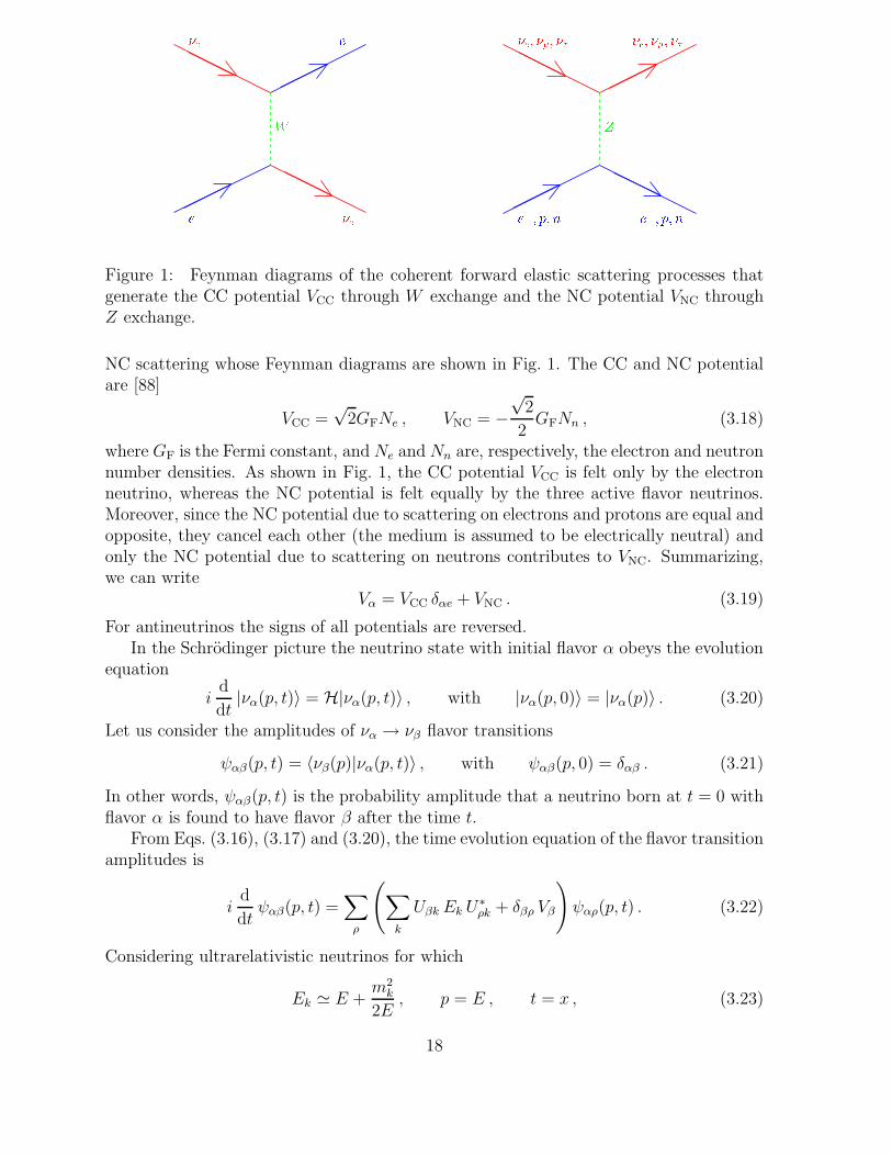
Figure 1: Feynman diagrams of the coherent forward elastic scattering processes thatgenerate the CC potential VCC through W exchange and the NC potential VNC throughZ exchange.

NC scattering whose Feynman diagrams are shown in Fig. 1. The CC and NC potentialare [88]

VCC =√

2GFNe , VNC = −√

2

2GFNn , (3.18)

where GF is the Fermi constant, and Ne and Nn are, respectively, the electron and neutronnumber densities. As shown in Fig. 1, the CC potential VCC is felt only by the electronneutrino, whereas the NC potential is felt equally by the three active flavor neutrinos.Moreover, since the NC potential due to scattering on electrons and protons are equal andopposite, they cancel each other (the medium is assumed to be electrically neutral) andonly the NC potential due to scattering on neutrons contributes to VNC. Summarizing,we can write

Vα = VCC δαe + VNC . (3.19)

For antineutrinos the signs of all potentials are reversed.In the Schrodinger picture the neutrino state with initial flavor α obeys the evolution

equation

id

dt|να(p, t)〉 = H|να(p, t)〉 , with |να(p, 0)〉 = |να(p)〉 . (3.20)

Let us consider the amplitudes of να → νβ flavor transitions

ψαβ(p, t) = 〈νβ(p)|να(p, t)〉 , with ψαβ(p, 0) = δαβ . (3.21)

In other words, ψαβ(p, t) is the probability amplitude that a neutrino born at t = 0 withflavor α is found to have flavor β after the time t.

From Eqs. (3.16), (3.17) and (3.20), the time evolution equation of the flavor transitionamplitudes is

id

dtψαβ(p, t) =

∑

ρ

(∑

k

Uβk Ek U∗ρk + δβρ Vβ

)ψαρ(p, t) . (3.22)

Considering ultrarelativistic neutrinos for which

Ek ≃ E +m2

k

2E, p = E , t = x , (3.23)

18

we have the evolution equation in space

id

dxψαβ(x) =

(p+

m21

2E+ VNC

)ψαβ(x) +

∑

ρ

(∑

k

Uβk∆m2

k1

2EU∗

ρk + δβe δρe VCC

)ψαρ(x) ,

(3.24)where we put in evidence the term (p+m2

1/2E + VNC)ψαβ(x) which generates a phasecommon to all flavors. This phase is irrelevant for the flavor transitions and can beeliminated by the phase shift

ψαβ(x) → ψαβ(x) e−i(p+m21/2E)x−i

∫ x

0VNC(x′) dx′

, (3.25)

which does not have any effect on the probability of να → νβ transitions,

Pνα→νβ(x) = |ψαβ(x)|2 . (3.26)

Therefore, the relevant evolution equation for the flavor transition amplitudes is

id

dxψαβ(x) =

∑

ρ

(∑

k

Uβk∆m2

k1

2EU∗

ρk + δβe δρe VCC

)ψαρ(x) , (3.27)

which shows that neutrino oscillation in matter, as neutrino oscillation in vacuum, de-pends on the differences of the squared neutrino masses, not on the absolute value ofneutrino masses. Equation (3.27) can be written in matrix form as

id

dxΨα =

1

2E

(U ∆M

2 U † + A)Ψα , (3.28)

with, in the case of three-neutrino mixing,

Ψα =

ψαe

ψαµ

ψατ

, ∆M2 =

0 0 00 ∆m2

21 00 0 ∆m2

31

, A =

ACC 0 0

0 0 00 0 0

, (3.29)

whereACC ≡ 2E VCC = 2

√2EGFNe . (3.30)

Since the case of three neutrino mixing is too complicated for an introductory discus-sion, let us consider the simplest case of two neutrino mixing between νe, νµ and ν1, ν2.Neglecting an irrelevant common phase, the evolution equation (3.28) can be written as

id

dx

(ψee

ψeµ

)=

1

4E

(−∆m2 cos 2ϑ+ 2ACC ∆m2 sin 2ϑ

∆m2 sin 2ϑ ∆m2 cos 2ϑ

)(ψee

ψeµ

), (3.31)

where ∆m2 ≡ m22 −m2

1 and ϑ is the mixing angle, such that

νe = cosϑ ν1 + sinϑ ν2 , νµ = − sin ϑ ν1 + cosϑ ν2 . (3.32)

If the initial neutrino is a νe, as in solar neutrino experiments, the initial condition forthe evolution equation (3.31) is

(ψee(0)ψeµ(0)

)=

(10

), (3.33)

19

and the probabilities of νe → νµ transitions and νe survival are

Pνe→νµ(x) = |ψeµ(x)|2 , Pνe→νe

(x) = |ψee(x)|2 = 1 − Pνe→νµ(x) . (3.34)

In practice the evolution equation of the flavor transition amplitudes can always besolved numerically with sufficient degree of precision given enough computational power.Let us discuss the analytical solution of Eq. (3.31) in the case of a matter density profilewhich is sufficiently smooth. This solution is useful in order to understand the qualitativeaspects of the problem.

The effective Hamiltonian matrix in Eq. (3.31) can be diagonalized by the orthogonaltransformation

Ψe = UM Ψ , with Ψe =

(ψee

ψeµ

), UM =

(cosϑM sinϑM

− sin ϑM cosϑM

), Ψ =

(ψ1

ψ2

),

(3.35)where ψk can be thought of as the amplitude of the effective massive neutrino νk inmatter (although such probability is not measurable, because only flavor neutrinos canbe detected). The angle ϑM is the effective mixing angle in matter, given by

tan 2ϑM =tan 2ϑ

1 − ACC

∆m2 cos 2ϑ

. (3.36)

The interesting new phenomenon, discovered by Mikheev and Smirnov in 1985 [89] (andbeautifully explained by Bethe in 1986 [90]) is that there is a resonance for

ACC = ∆m2 cos 2ϑ , (3.37)

which corresponds to the electron number density

NRe =

∆m2 cos 2ϑ

2√

2EGF

. (3.38)

In the resonance the effective mixing angle is equal to 45, i.e. the mixing is maximal,leading to the possibility of total transitions between the two flavors if the resonanceregion is wide enough. This mechanism is called “MSW effect” in honor of Mikheev,Smirnov and Wolfenstein.

The effective squared-mass difference in matter is

∆m2M =

√(∆m2 cos 2ϑ− ACC)2 + (∆m2 sin 2ϑ)2 . (3.39)

Neglecting an irrelevant common phase, the evolution equation for the amplitudes ofthe effective massive neutrinos in matter is

id

dx

(ψ1

ψ2

)=

[1

4E

(−∆m2

M 00 ∆m2

M

)+

(0 −idϑM/dx

idϑM/dx 0

)](ψ1

ψ2

), (3.40)

with the initial condition(ψ1(0)ψ2(0)

)=

(cosϑ0

M − sinϑ0M

sinϑ0M cosϑ0

M

)(10

)=

(cosϑ0

M

sinϑ0M

), (3.41)

20

e ' 2 ' 1e ' 1 ' 2

NRe =NA

Ne=NA ( m3)# M

100806040200

90807060504030201002

2e 1

1 eNRe =NA

Ne=NA ( m3)m2 M(106 eV2 )

100806040200

14121086420Figure 2: Effective mixing angle ϑM (left) and effective squared-mass difference ∆m2

M

(right) in matter as functions of the electron number density Ne divided by the Avogadronumber NA, for ∆m2 = 7 × 10−6 eV2, sin2 2ϑ = 10−3. NR

e ≡ ∆m2 cos 2ϑ/2√

2EGF is theelectron number density at the resonance, where ϑM = 45.

where ϑ0M is the effective mixing angle in matter at the point of neutrino production.

If the matter density is constant, dϑM/dx = 0 and the evolutions of the amplitudes ofthe effective massive neutrinos in matter are decoupled, leading to the transition proba-bility

Pνe→νµ(x) = sin2 2ϑM sin2

(∆m2

Mx

4E

), (3.42)

which has the same structure as the two-neutrino transition probability in vacuum (3.12),with the mixing angle and the squared-mass difference replaced by their effective valuesin matter.

If the matter density is not constant, it is necessary to take into account the effect ofdϑM/dx,

dϑM

dx=

1

2

∆m2 sin 2ϑ

(∆m2 cos 2ϑ−ACC)2 + (∆m2 sin 2ϑ)2

dACC

dx, (3.43)

which is maximum at the resonance,

dϑM

dx

∣∣∣∣R

=1

2 tan 2ϑ

d lnNe

dx

∣∣∣∣R

. (3.44)

This is illustrated in the left panel of Fig. 2 for ∆m2 = 7×10−6 eV2, sin2 2ϑ = 10−3. Onecan see that for Ne ≪ NR

e the effective mixing angle is practically equal to the mixingangle in vacuum, ϑM ≃ ϑ, for Ne ≃ NR

e the effective mixing angle varies very rapidlywith the electron number density, passing through 45 at Ne = NR

e and going rapidly to90 for Ne > NR

e .The right panel of Fig. 2 shows the corresponding behavior of the effective squared-

mass difference ∆m2M, which is useful in order to understand how the presence of a

resonance can induce an almost complete νe → νµ conversion of solar neutrinos. If themixing parameters are such that at the center of the sun Ne ≫ NR

e , the effective mixingangle is practically 90 and electron neutrinos are produced as almost pure ν2. As theneutrino propagates out of the sun, it crosses the resonance at Ne = NR

e , where theenergy gap between ν1 and ν2 is minimum. If the resonance is crossed adiabatically, the

21

neutrino remains ν2 and exits the sun as ν2 = sinϑ νe +cosϑ νµ, which is almost equal toνµ if the mixing angle is small, leading to almost complete νe → νµ conversion. This isthe case in which the MSW effect is most effective and striking, since a large conversionis achieved in spite of a small mixing angle.

If the resonance is not crossed adiabatically, ν2 → ν1 transitions occur in an intervalaround the resonance and the neutrino emerges out of the sun as a mixture of ν2 and ν1,leading to partial conversion of νe into νµ. Quantitatively, we can write the amplitudesof ν1 and ν2 at any point x after resonance crossing as

ψ1(x) =

[cosϑ0

M exp

(i

∫ xR

0

∆m2M(x′)

4Edx′)AR

11 + sinϑ0M exp

(−i∫ xR

0

∆m2M(x′)

4Edx′)AR

21

]

× exp

(i

∫ x

xR

∆m2M(x′)

4Edx′), (3.45)

ψ2(x) =

[cosϑ0

M exp

(i

∫ xR

0

∆m2M(x′)

4Edx′)AR

12 + sinϑ0M exp

(−i∫ xR

0

∆m2M(x′)

4Edx′)AR

22

]

× exp

(−i∫ x

xR

∆m2M(x′)

4Edx′), (3.46)

where ARkj is the amplitude of νk → νj transitions in the resonance.

Considering x as the detection point on the earth, practically in vacuum, the proba-bility of νe survival is given by

P νe→νe(x) = |ψee(x)|2 , with ψee(x) = cosϑψ1(x) + sinϑψ2(x) . (3.47)

If ∆m2 ≫ 10−10 eV2 all the phases in Eqs. (3.45) and (3.46) are very large and rapidlyoscillating as functions of the neutrino energy. In this case, the average of the transitionprobability over the energy resolution of the detector washes out all interference termsand only the averaged survival probability

Psun

νe→νe= cos2 ϑ cos2 ϑ0

M |AR11|2 + cos2 ϑ sin2 ϑ0

M |AR21|2

+ sin2 ϑ cos2 ϑ0M |AR

12|2 + sin2 ϑ sin2 ϑ0M |AR

22|2 , (3.48)

which is independent from the sun–earth distance, is measurable. Taking into accountthat conservation of probability implies that

|AR11|2 = |AR

22|2 = 1 − Pc , |AR12|2 = |AR

21|2 = Pc , (3.49)

where Pc is the ν1 ν2 crossing probability at the resonance, we obtain the so-calledParke formula [91] for the averaged νe survival probability:

Psun

νe→νe=

1

2+

(1

2− Pc

)cos 2ϑ0

M cos 2ϑ . (3.50)

This formula has been widely used for the analysis of solar neutrino data.The main problem in the application of the Parke formula (3.50) is the calculation of

the crossing probability. This probability must involve the energy gap ∆m2M/2E between

22

ν1 and ν2 and the off diagonal terms proportional to dϑM/dx in Eq. (3.40), which causethe ν1 ν2 transitions. Indeed, the crossing probability can be written as [92, 93, 94, 95]

Pc =exp

(−π

2γF)− exp

(−π

2γ F

sin2 ϑ

)

1 − exp(−π

2γ F

sin2 ϑ

) , (3.51)

where γ is the adiabaticity parameter

γ =∆m2

M/2E

2|dϑM/dx|

∣∣∣∣R

=∆m2 sin2 2ϑ

2E cos 2ϑ |d lnNe/dx|R. (3.52)

If γ is large, the resonance is crossed adiabatically and Pc ≪ 1, leading to

Psun, adiabatic

νe→νe=

1

2+

1

2cos 2ϑ0

M cos 2ϑ . (3.53)

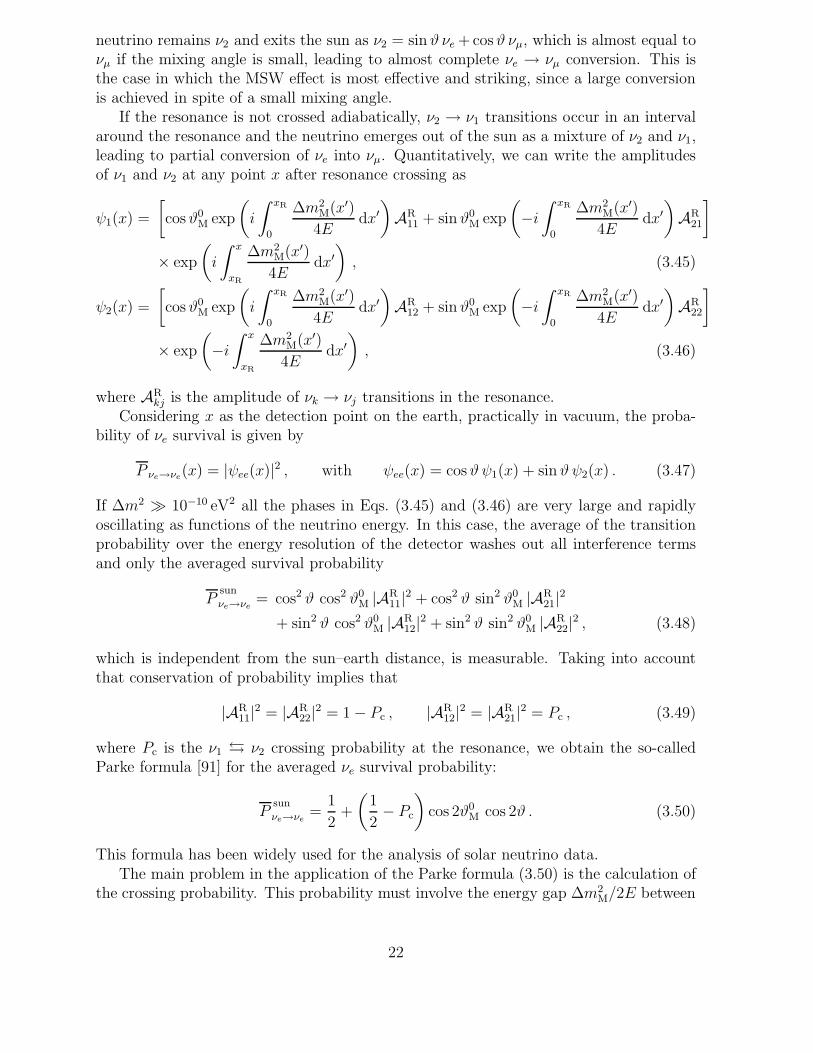
The parameter F in Eq. (3.51) depends on the electron density profile. The left panel inFigure 3 shows the Standard Solar Model (SSM) electron density profile in the sun [96],which is well approximated by the exponential

Ne(R) = Ne(0) exp

(− R

R0

), with Ne(0) = 245NA/cm

3 , and R0 =R⊙

10.54,

(3.54)where R is the distance from the center of the sun and R⊙ is the solar radius. For anexponential electron density profile the parameter F is given by [92, 93, 94, 97, 98, 99]

F = 1 − tan2 ϑ . (3.55)

For |d lnNe/dx|R the authors of Ref. [100] suggested the practical prescription, verifiedwith numerical solutions of the differential evolution equation, to calculate it numericallyfrom the SSM electron density profile for R ≤ 0.904R⊙ and take the constant value18.9/R⊙ for R > 0.904R⊙, where the exponential approximation (3.54) breaks down.

For the analysis of solar neutrino data it is also necessary to take into account thematter effect along the propagation of neutrinos in the earth during the night (the so-called “νe regeneration in the earth”), which can generate a day-night asymmetry of therates. The probability of solar νe survival after crossing the earth is given by [18, 101]

P sun+earthνe→νe

= Psun

νe→νe+

(1 − 2P

sun

νe→νe

) (P earth

ν2→νe− sin2 ϑ

)

cos2ϑ. (3.56)

Since the earth density profile is not a smooth function, the probability P earthν2→νe

must becalculated numerically. A good approximation is obtained by approximating the earthdensity profile with a step function (see Refs. [102, 103, 104, 105, 106]). According toEq. (3.40), the effective massive neutrinos propagate as plane waves in regions of constantdensity, with a phase exp (±i∆m2

M∆x/4E), where ∆x is the width of the step. At theboundaries of steps the wave functions of flavor neutrinos are joined, according to thescheme

Ψ(xn) =[UM Φ(xn − xn−1)U

†M

]

(n)

[UM Φ(xn−1 − xn−2)U

†M

]

(n−1)

23

SMA

VACQVO

LOWLMA

tan2 #

m2(eV2 )

101100101102103104

103104105106107108109101010111012Figure 3: Left: Standard Solar Model electron density profile in the sun as a function ofthe ratio R/R⊙ [96]. The straight line represents the approximation in Eq. (3.54). Right:The conventional names for regions in the tan2 ϑ–∆m2 plane obtained from the analysisof solar neutrino data. The vertical dotted line correspond to maximal mixing.

. . .[UM Φ(x2 − x1)U

†M

]

(2)

[UM Φ(x1 − x0)U

†M

]

(1)U Ψ(x0) . (3.57)

where x0 is the coordinate of the point in which the neutrino enters the earth, x1, x2, . . . ,xn are the boundaries of n steps with which the earth density profile is approximated,Φ(∆x) = diag(exp (−i∆m2

M∆x/4E) , exp (i∆m2M∆x/4E)), and the notation [. . .](i) indi-

cates that all the matter-dependent quantities in the square brackets must be evaluatedwith the matter density in the ith step, that extends from xi−1 to xi.

The right panel in Fig. 3 shows the conventional names for regions in the tan2 ϑ–∆m2

plane obtained from the analysis of solar neutrino data. The Small Mixing Angle (SMA)region is the one where the mixing angle is very small and the resonant enhancementof flavor transitions due to the MSW effect is more efficient. However, as explained inSection 4.1 there is currently a very strong evidence in favor of the Large Mixing Angle(LMA) region, in which both the mixing angle and ∆m2 are large. Other regions withlarge mixing are: the low ∆m2 (LOW) region, the Quasi-Vacuum-Oscillations (QVO)region, and the VACuum Oscillations region (VAC). In the SMA, LMA and LOW regionsvacuum oscillations due to the sun–earth distance are not observable because the ∆m2 istoo high and interference effects are washed out by the average over the energy resolutionof the detector (in these cases the Parke formula (3.50) applies). In the QVO region bothmatter effects and vacuum oscillations are important [107, 108, 109, 100]. In the VACregion matter effects are negligible and vacuum oscillations are dominant.

Concluding this Section on the theory of neutrino oscillations, let us mention that theevolution equation (3.28) allows to prove easily that the Majorana phases in the mixingmatrix do not have any effect on neutrino oscillations in vacuum [110, 111] as well as inmatter [112], because the diagonal matrix of Majorana phases D(λ21, λ31) on the right ofthe mixing matrix in Eq. (2.48) cancels in the product U∆M2U †. Therefore, the Dirac

24

Experiment Channels

Bugey νe → νe [64]

CDHS(−)

ν µ → (−)

ν µ [71]

CCFR(−)

ν µ → (−)

ν µ [113],(−)

ν µ → (−)

ν e [72],(−)

ν e →(−)

ν τ [72](−)

ν e →(−)

ν e [72]LSND νµ → νe [75], νµ → νe [114],

KARMEN νµ → νe [76]NOMAD νµ → νe [74] νµ → ντ [115], νe → ντ [115]CHORUS νµ → ντ [73], νe → ντ [73]

NuTeV(−)

ν µ → (−)

ν e [116]

Table 1: Short-baseline experiments (SBL) whose data give the most stringent constraintson different oscillation channels.

or Majorana nature of neutrinos cannot be distinguished in neutrino oscillations.

4 Neutrino oscillation experiments

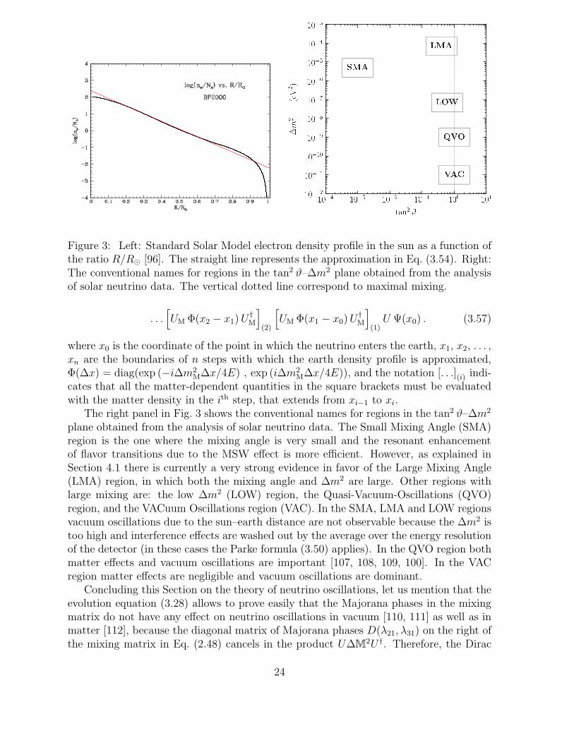
In this Section we review the main results of the oscillation experiments which are con-nected with the existing model-independent evidences in favor of oscillations of solar andatmospheric neutrinos and the interpretation of the experimental data in the frameworkof three neutrino mixing, discussed in Section 5. We do not discuss the results of severalshort-baseline neutrino (SBL) oscillation experiments, which have probed scales of ∆m2

bigger than about 0.1 eV2, that are larger than the scales of ∆m2 indicated by solar andatmospheric neutrino data. The SBL experiments whose data give the most stringentconstraints on the different oscillation channels are listed in Table 1.

All the SBL experiments in Table 1 did not observe any indication of neutrino oscil-lations, except the LSND experiment [114, 75]. A large part of the region in the sin2 2ϑ–∆m2 plane allowed by LSND has been excluded by the results of other experimentswhich are sensitive to similar values of the neutrino oscillation parameters (KARMEN[76], CCFR [117], NOMAD [74]; see Ref. [118] for an accurate combined analysis of LSNDand KARMEN data). The MiniBooNE experiment [119] running at Fermilab will tell usthe validity of the LSND indication in the near future.

Some years ago the oscillations indicated by the LSND experiment could be accom-modated together with solar and atmospheric neutrino oscillations in the framework offour-neutrino mixing, in which there are three light active neutrinos and one light sterileneutrino (see Refs. [21, 120, 121, 122] and references in Ref. [39]). However, the globalfit of recent data in terms of four-neutrino mixing is not good [123], disfavoring suchpossibility. Therefore, in this review we discuss only three-neutrino mixing, which cannotexplain the LSND indication, awaiting the response of MiniBooNE before engaging inwild speculations (see Refs. [124, 125, 126, 127, 128, 129, 130, 131]).

25

4.1 Solar neutrino experiments and KamLAND

At the end of the 60’s the radiochemical Homestake experiment [9] began the observationof solar neutrinos through the charged-current reaction [132, 133]

νe + 37Cl → 37Ar + e− , (4.1)

with a threshold EClth = 0.814 MeV which allows to observe mainly 7Be and 8B neutrinos

produced, respectively, in the reactions e− + 7Be → 7Li + νe (E = 0.8631 MeV) and8B → 8Be∗ + e+ + νe (E . 15 MeV) of the thermonuclear pp cycle that produces energyin the core of the sun (see Refs. [134, 15]).

The Homestake experiment is called “radiochemical” because the 37Ar atoms wereextracted every ∼35 days from the detector tank containing 615 tons of tetrachloroethy-lene (C2Cl4) through chemical methods and counted in small proportional counters whichdetect the Auger electron produced in the electron-capture of 37Ar. As all solar neutrinodetectors, the Homestake tank was located deep underground (1478 m) in order to havea good shielding from cosmic ray muons. The Homestake experiment detected solar elec-tron neutrinos for about 30 years [9], measuring a flux which is about one third of theone predicted Standard Solar Model (SSM) [96]:

ΦHomCl

ΦSSMCl

= 0.34 ± 0.03 . (4.2)

This deficit was called “the solar neutrino problem”.The solar neutrino problem was confirmed in the late 80’s by the real-time water

Cherenkov Kamiokande experiment [85] (3000 tons of water, 1000 m underground) whichobserved solar neutrinos through the elastic scattering (ES) reaction

ν + e− → ν + e− , (4.3)

which is mainly sensitive to electron neutrinos, whose cross section is about six time largerthan the cross section of muon and tau neutrinos. The experiment is called “real-time”because the Cherenkov light produced in water by the recoil electron in the reaction(4.3) is observed in real time. The solar neutrino signal is separated statistically fromthe background using the fact that the recoil electron preserves the directionality of theincoming neutrino. The energy threshold of the Kamiokande experiment was 6.75 MeV,allowing only the detection of 8B neutrinos. After 1995 the Kamiokande experimenthas been replaced by the bigger Super-Kamiokande experiment [8, 66, 67] (50 ktons ofwater, 1000 m underground) which has measured with high accuracy the flux of solar 8Bneutrinos with an energy threshold of 4.75 MeV, obtaining [66]

ΦS-KES

ΦSSMES

= 0.465 ± 0.015 . (4.4)

In the early 90’s the GALLEX [61] (30.3 tons of 71Ga, 1400 m underground) andSAGE [62] (50 tons of 71Ga, 2000 m underground) radiochemical experiments started theobservation of solar electron neutrinos through the charged-current reaction [135]

νe + 71Ga → 71Ge + e− , (4.5)

26

which has the low energy threshold of 0.233 MeV, that allows the detection of the so-calledpp neutrinos produced in the main reaction p + p → d + e+ + νe (E . 0.42 MeV) of thepp cycle, besides the 7Be, 8B and other neutrinos. After 1997 the GALLEX experimenthas been upgraded, changing its name to GNO [63]. The combined results of the threeGallium experiments confirm the solar neutrino problem:

ΦGa

ΦSSMGa

= 0.56 ± 0.03 . (4.6)

Although it was difficult to doubt of the Standard Solar Model, which was well testedby helioseismological measurements (see Ref. [136]), and it was difficult to explain thedifferent suppression of solar νe’s observed in different experiments with astrophysicalmechanisms, a definitive model-independent proof that the solar neutrino problem is dueto neutrino physics was lacking until the real-time heavy-water Cherenkov detector SNO[7, 10, 11] (1 kton of D2O, 2073 m underground) observed solar 8B neutrinos through thecharged-current (CC) reaction

νe + d→ p+ p+ e− , (4.7)

with ESNOth,CC = 8.2 MeV and the neutral-current (NC) reaction

ν + d→ p+ n+ ν , (4.8)

with ESNOth,NC = 2.2 MeV, besides the ES reaction (4.3) with ESNO

th,ES = 7.0 MeV. The obser-vation of solar neutrinos through the CC and NC reactions has provided the breakthroughfor the definitive solution of the solar neutrino problem in favor of new neutrino physics.The charged-current reaction is very important because it allows to measure with highstatistics the energy spectrum of solar νe’s. The neutral current reaction is extremelyimportant for the measurement of the total flux of active νe, νµ and ντ , which interactwith the same cross section.

In June 2001 the combination of the first SNO CC data [7] and the high-precisionSuper-Kamiokande ES data [8] allowed to extract a model-independent indication of theoscillations of solar electron neutrinos into active νµ’s and/or ντ ’s [7] (see also Refs. [137,138]). In April 2002 the observation of solar neutrinos through the NC and CC reactionsallowed the SNO experiment [10] to solve definitively the long-standing solar neutrinoproblem in favor of the existence of νe → νµ, ντ transitions. In this first phase [10], called“D2O phase”, the neutron produced in the neutral-current reaction (4.8) was detectedby observing the photon produced in the reaction

n+ d→ 3H + γ (Eγ = 6.25 MeV) . (4.9)

In September 2003 the SNO collaboration released the data obtained in the second phase[11], called “salt phase”, in which 2 tons of salt has been added to the heavy water inthe SNO detector, allowing the detection of the neutron produced in the neutral-currentreaction (4.8) by observing the photons produced in the reaction

n+ 35Cl → 36Cl + several γ’s (Etotγ = 8.6 MeV) . (4.10)

The better signature given by several photons and the higher cross-section of reaction(4.10) with respect to reaction (4.9) have allowed the SNO collaboration to measure with

27

θ2tan

)2 (

eV2

m∆

10-5

10-4

10-1

1θ22sin

0 0.2 0.4 0.6 0.8 1

)2 (

eV2

m∆

10-6

10-5

10-4

10-3

Rate excludedRate+Shape allowedLMAPalo Verde excludedChooz excluded

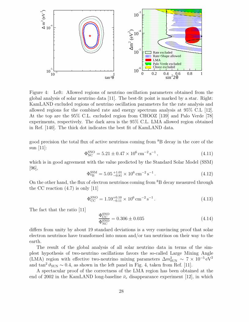
Figure 4: Left: Allowed regions of neutrino oscillation parameters obtained from theglobal analysis of solar neutrino data [11]. The best-fit point is marked by a star. Right:KamLAND excluded regions of neutrino oscillation parameters for the rate analysis andallowed regions for the combined rate and energy spectrum analysis at 95% C.L [12].At the top are the 95% C.L. excluded region from CHOOZ [139] and Palo Verde [78]experiments, respectively. The dark area is the 95% C.L. LMA allowed region obtainedin Ref. [140]. The thick dot indicates the best fit of KamLAND data.

good precision the total flux of active neutrinos coming from 8B decay in the core of thesun [11]:

ΦSNONC = 5.21 ± 0.47 × 106 cm−2 s−1 , (4.11)

which is in good agreement with the value predicted by the Standard Solar Model (SSM)[96],

ΦSSM8B = 5.05 +1.01

−0.81 × 106 cm−2 s−1 . (4.12)

On the other hand, the flux of electron neutrinos coming from 8B decay measured throughthe CC reaction (4.7) is only [11]

ΦSNOCC = 1.59+0.10

−0.11 × 106 cm−2 s−1 . (4.13)

The fact that the ratio [11]ΦSNO

CC

ΦSNONC

= 0.306 ± 0.035 (4.14)

differs from unity by about 19 standard deviations is a very convincing proof that solarelectron neutrinos have transformed into muon and/or tau neutrinos on their way to theearth.

The result of the global analysis of all solar neutrino data in terms of the sim-plest hypothesis of two-neutrino oscillations favors the so-called Large Mixing Angle(LMA) region with effective two-neutrino mixing parameters ∆m2

SUN ∼ 7 × 10−5 eV2

and tan2 ϑSUN ∼ 0.4, as shown in the left panel in Fig. 4, taken from Ref. [11].A spectacular proof of the correctness of the LMA region has been obtained at the

end of 2002 in the KamLAND long-baseline νe disappearance experiment [12], in which

28

the suppressionNKamLAND

observed

NKamLANDexpected

= 0.611 ± 0.094 . (4.15)

of the νe flux produced by nuclear reactors at an average distance of about 180 km wasobserved. The right panel in Fig. 4 shows the regions of oscillation parameters allowedby KamLAND, compared with the allowed LMA region obtained in Ref. [140] in 2002after the release of the data of the first D2O phase of the SNO experiment [10]. Fromthe right panel in Fig. 4 one can see that the LMA region and the KamLAND allowedregions overlap in two subregions at ∆m2

SUN ≃ 7×10−5 eV2 and ∆m2SUN ≃ 1.5×10−4 eV2.

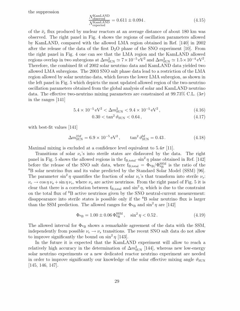
Therefore, the combined fit of 2002 solar neutrino data and KamLAND data yielded twoallowed LMA subregions. The 2003 SNO salt phase data lead to a restriction of the LMAregion allowed by solar neutrino data, which favors the lower LMA subregion, as shown inthe left panel in Fig. 5 which depicts the most updated allowed region of the two-neutrinooscillation parameters obtained from the global analysis of solar and KamLAND neutrinodata. The effective two-neutrino mixing parameters are constrained at 99.73% C.L. (3σ)in the ranges [141]

5.4 × 10−5 eV2 < ∆m2SUN < 9.4 × 10−5 eV2 , (4.16)

0.30 < tan2 ϑSUN < 0.64 , (4.17)

with best-fit values [141]

∆m2 bfSUN = 6.9 × 10−5 eV2 , tan2 ϑbf

SUN = 0.43 . (4.18)

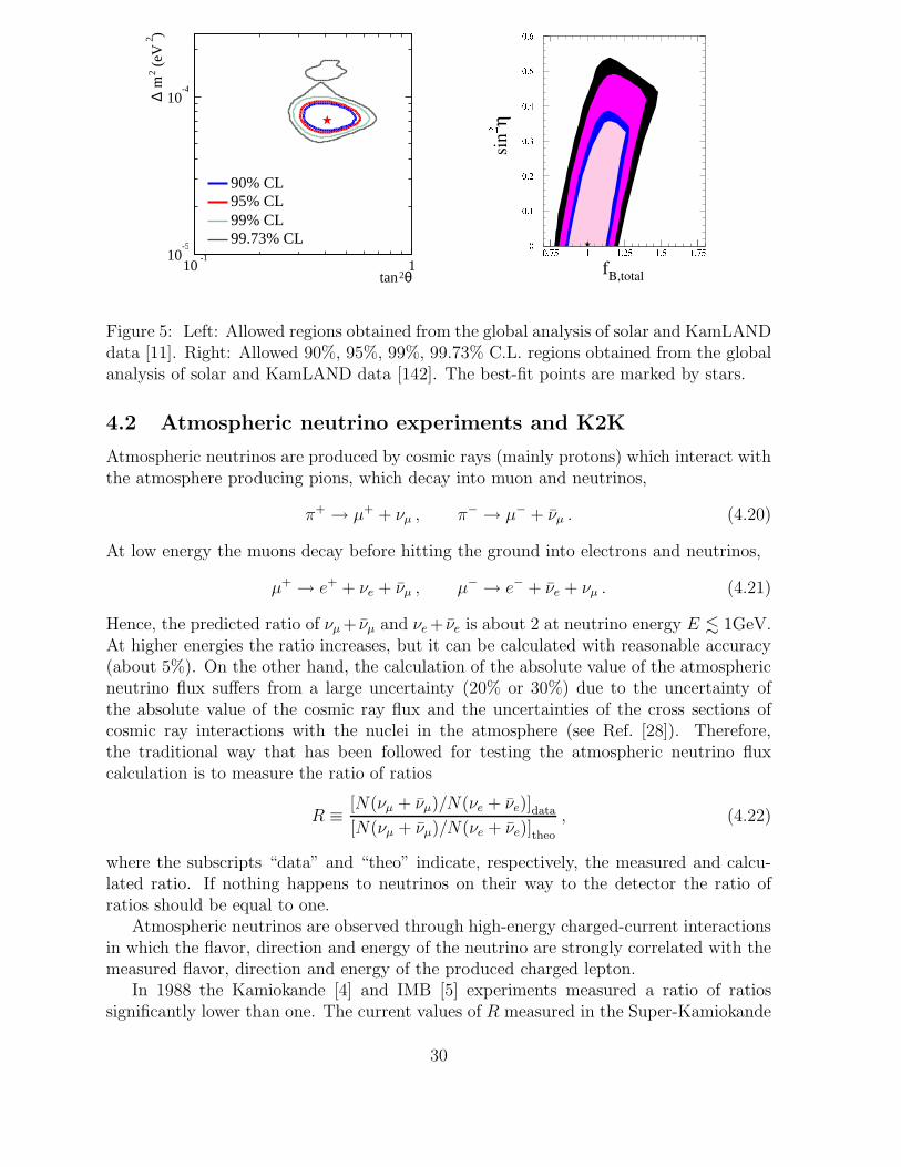
Maximal mixing is excluded at a confidence level equivalent to 5.4σ [11].Transitions of solar νe’s into sterile states are disfavored by the data. The right

panel in Fig. 5 shows the allowed regions in the fB,total–sin2 η plane obtained in Ref. [142]before the release of the SNO salt data, where fB,total = Φ8B/Φ

SSM8B is the ratio of the

8B solar neutrino flux and its value predicted by the Standard Solar Model (SSM) [96].The parameter sin2 η quantifies the fraction of solar νe’s that transform into sterile νs:νe → cos η νa + sin η νs, where νa are active neutrinos. From the right panel of Fig. 5 it isclear that there is a correlation between fB,total and sin2 η, which is due to the constrainton the total flux of 8B active neutrinos given by the SNO neutral-current measurement:disappearance into sterile states is possible only if the 8B solar neutrino flux is largerthan the SSM prediction. The allowed ranges for Φ8B and sin2 η are [142]

Φ8B = 1.00 ± 0.06 ΦSSM8B , sin2 η < 0.52 . (4.19)

The allowed interval for Φ8B shows a remarkable agreement of the data with the SSM,independently from possible νe → νs transitions. The recent SNO salt data do not allowto improve significantly the bound on sin2 η [143].

In the future it is expected that the KamLAND experiment will allow to reach arelatively high accuracy in the determination of ∆m2

SUN [144], whereas new low-energysolar neutrino experiments or a new dedicated reactor neutrino experiment are neededin order to improve significantly our knowledge of the solar effective mixing angle ϑSUN

[145, 146, 147].

29

)2 (

eV2

m∆

10-5

10-4

10θ2tan

10-1

1

90% CL95% CL99% CL99.73% CL

Figure 5: Left: Allowed regions obtained from the global analysis of solar and KamLANDdata [11]. Right: Allowed 90%, 95%, 99%, 99.73% C.L. regions obtained from the globalanalysis of solar and KamLAND data [142]. The best-fit points are marked by stars.

4.2 Atmospheric neutrino experiments and K2K

Atmospheric neutrinos are produced by cosmic rays (mainly protons) which interact withthe atmosphere producing pions, which decay into muon and neutrinos,

π+ → µ+ + νµ , π− → µ− + νµ . (4.20)

At low energy the muons decay before hitting the ground into electrons and neutrinos,

µ+ → e+ + νe + νµ , µ− → e− + νe + νµ . (4.21)

Hence, the predicted ratio of νµ + νµ and νe + νe is about 2 at neutrino energy E . 1GeV.At higher energies the ratio increases, but it can be calculated with reasonable accuracy(about 5%). On the other hand, the calculation of the absolute value of the atmosphericneutrino flux suffers from a large uncertainty (20% or 30%) due to the uncertainty ofthe absolute value of the cosmic ray flux and the uncertainties of the cross sections ofcosmic ray interactions with the nuclei in the atmosphere (see Ref. [28]). Therefore,the traditional way that has been followed for testing the atmospheric neutrino fluxcalculation is to measure the ratio of ratios

R ≡ [N(νµ + νµ)/N(νe + νe)]data

[N(νµ + νµ)/N(νe + νe)]theo

, (4.22)

where the subscripts “data” and “theo” indicate, respectively, the measured and calcu-lated ratio. If nothing happens to neutrinos on their way to the detector the ratio ofratios should be equal to one.

Atmospheric neutrinos are observed through high-energy charged-current interactionsin which the flavor, direction and energy of the neutrino are strongly correlated with themeasured flavor, direction and energy of the produced charged lepton.

In 1988 the Kamiokande [4] and IMB [5] experiments measured a ratio of ratiossignificantly lower than one. The current values of R measured in the Super-Kamiokande

30

10-1

1 10 102

-1

-0.5

0

0.5

1

10-1

1 10

-1

-0.5

0

0.5

1

e-like

µ-like

FC PC

(U-D

)/(U

+D

)

Momentum (GeV/c)

νµ - ντ

10-4

10-3

10-2

10-1

0 0.1 0.2 0.3 0.4 0.5 0.6 0.7 0.8 0.9 1

68% C.L.90% C.L.99% C.L.

sin22θ

∆m2 (

eV2 )

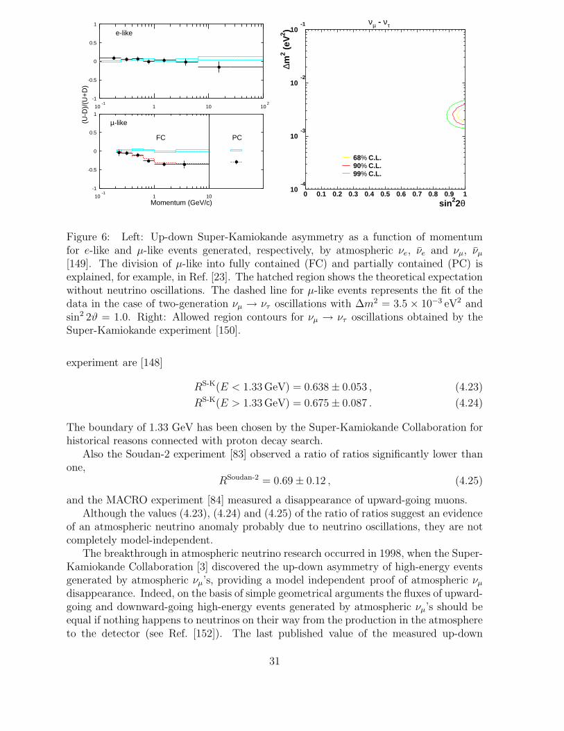
Figure 6: Left: Up-down Super-Kamiokande asymmetry as a function of momentumfor e-like and µ-like events generated, respectively, by atmospheric νe, νe and νµ, νµ

[149]. The division of µ-like into fully contained (FC) and partially contained (PC) isexplained, for example, in Ref. [23]. The hatched region shows the theoretical expectationwithout neutrino oscillations. The dashed line for µ-like events represents the fit of thedata in the case of two-generation νµ → ντ oscillations with ∆m2 = 3.5 × 10−3 eV2 andsin2 2ϑ = 1.0. Right: Allowed region contours for νµ → ντ oscillations obtained by theSuper-Kamiokande experiment [150].

experiment are [148]

RS-K(E < 1.33 GeV) = 0.638 ± 0.053 , (4.23)

RS-K(E > 1.33 GeV) = 0.675 ± 0.087 . (4.24)

The boundary of 1.33 GeV has been chosen by the Super-Kamiokande Collaboration forhistorical reasons connected with proton decay search.

Also the Soudan-2 experiment [83] observed a ratio of ratios significantly lower thanone,

RSoudan-2 = 0.69 ± 0.12 , (4.25)

and the MACRO experiment [84] measured a disappearance of upward-going muons.Although the values (4.23), (4.24) and (4.25) of the ratio of ratios suggest an evidence

of an atmospheric neutrino anomaly probably due to neutrino oscillations, they are notcompletely model-independent.

The breakthrough in atmospheric neutrino research occurred in 1998, when the Super-Kamiokande Collaboration [3] discovered the up-down asymmetry of high-energy eventsgenerated by atmospheric νµ’s, providing a model independent proof of atmospheric νµ

disappearance. Indeed, on the basis of simple geometrical arguments the fluxes of upward-going and downward-going high-energy events generated by atmospheric νµ’s should beequal if nothing happens to neutrinos on their way from the production in the atmosphereto the detector (see Ref. [152]). The last published value of the measured up-down

31

MACRO

SOUDAN 2SK

∆m2

(eV

2 )10-1

10-2

10-3

10-4

10-50 0.2 0.4 0.6 0.8 1.0

sin2 (2θ)

10-4

10-3

10-2

0 0.1 0.2 0.3 0.4 0.5 0.6 0.7 0.8 0.9 1sin22θ

∆m2 (e

V2 )

68%90%99%

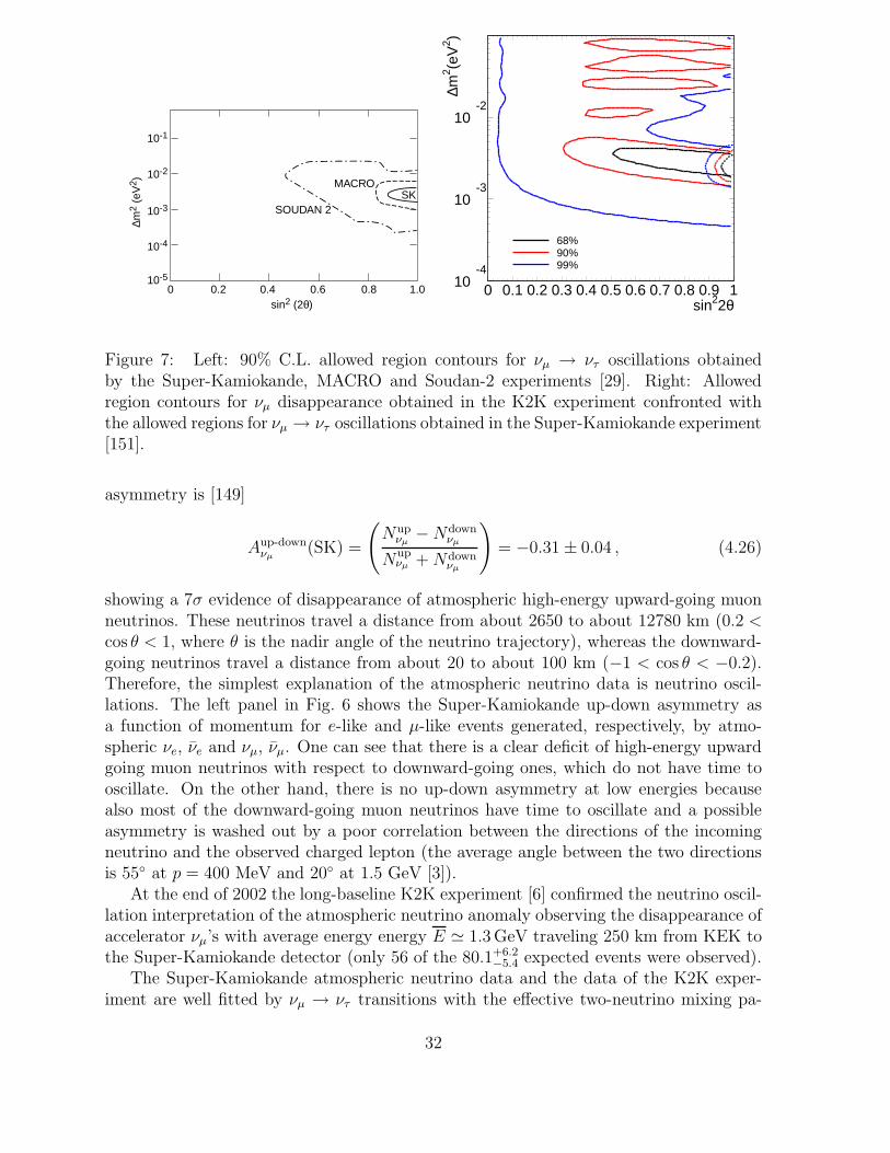
Figure 7: Left: 90% C.L. allowed region contours for νµ → ντ oscillations obtainedby the Super-Kamiokande, MACRO and Soudan-2 experiments [29]. Right: Allowedregion contours for νµ disappearance obtained in the K2K experiment confronted withthe allowed regions for νµ → ντ oscillations obtained in the Super-Kamiokande experiment[151].

asymmetry is [149]

Aup-downνµ

(SK) =

(Nup

νµ−Ndown

νµ

Nupνµ +Ndown

νµ

)= −0.31 ± 0.04 , (4.26)

showing a 7σ evidence of disappearance of atmospheric high-energy upward-going muonneutrinos. These neutrinos travel a distance from about 2650 to about 12780 km (0.2 <cos θ < 1, where θ is the nadir angle of the neutrino trajectory), whereas the downward-going neutrinos travel a distance from about 20 to about 100 km (−1 < cos θ < −0.2).Therefore, the simplest explanation of the atmospheric neutrino data is neutrino oscil-lations. The left panel in Fig. 6 shows the Super-Kamiokande up-down asymmetry asa function of momentum for e-like and µ-like events generated, respectively, by atmo-spheric νe, νe and νµ, νµ. One can see that there is a clear deficit of high-energy upwardgoing muon neutrinos with respect to downward-going ones, which do not have time tooscillate. On the other hand, there is no up-down asymmetry at low energies becausealso most of the downward-going muon neutrinos have time to oscillate and a possibleasymmetry is washed out by a poor correlation between the directions of the incomingneutrino and the observed charged lepton (the average angle between the two directionsis 55 at p = 400 MeV and 20 at 1.5 GeV [3]).

At the end of 2002 the long-baseline K2K experiment [6] confirmed the neutrino oscil-lation interpretation of the atmospheric neutrino anomaly observing the disappearance ofaccelerator νµ’s with average energy energy E ≃ 1.3 GeV traveling 250 km from KEK tothe Super-Kamiokande detector (only 56 of the 80.1+6.2

−5.4 expected events were observed).The Super-Kamiokande atmospheric neutrino data and the data of the K2K exper-

iment are well fitted by νµ → ντ transitions with the effective two-neutrino mixing pa-

32

rameters constrained in the ranges [153]

1.4 × 10−3 eV2 < ∆m2ATM < 5.1 × 10−3 eV2 , (4.27)

sin2 2ϑATM > 0.86 , (4.28)

at 99.73% C.L. (3σ), with best-fit values

∆m2 bfATM = 2.6 × 10−3 eV2 , sin2 2ϑbf

ATM = 1 . (4.29)

Hence, the best-fit effective atmospheric mixing is maximal. The right panel in Fig. 6shows the region in the sin2 2ϑATM–∆m2

ATM plane for νµ → ντ oscillations allowed bySuper-Kamiokande data [150]. The left panel in Fig. 7 shows the 90% C.L. allowed regionsfor νµ → ντ oscillations obtained in the MACRO and Soudan-2 experiments confrontedwith the corresponding region obtained in the Super-Kamiokande experiment [29]. Theright panel in Fig. 7 shows the allowed regions for νµ disappearance obtained in the K2Kexperiment confronted with the allowed regions for νµ → ντ oscillations obtained in theSuper-Kamiokande experiment [151]. The left panel in Fig. 8 shows the allowed regionobtained in Ref. [153] from the combined analysis of Super-Kamiokande atmospheric andK2K data.

Transitions of atmospheric νµ’s into νe’s or sterile states are disfavored. The fractionsin2 ξ of atmospheric νµ’s that transform into sterile νs (νµ → cos ξ ντ +sin ξ νs) is limitedat 90% C.L. by [154]

sin2 ξ < 0.19 . (4.30)

In the next years the MINOS [79] experiment will measure with improved precisionthe disappearance of muon neutrinos over a long-baseline of about 730 km. The OPERA[155] and ICARUS [156] experiments belonging to the CERN to Gran Sasso program(CNGS) [80] are aimed at a direct measurement of νµ → ντ oscillation over a similarlong-baseline of about 730 km.

4.3 The reactor experiment CHOOZ

CHOOZ was a long-baseline reactor νe disappearance experiment [157, 139, 77] whichdid not observe any disappearance of electron neutrinos at a distance of about 1 km fromthe source. In spite of such negative result, the CHOOZ experiment is very important,because it shows that the oscillations of electron neutrinos at the atmospheric scale of∆m2 are small or zero. This constraint is particularly important in the framework ofthree-neutrino mixing, as will be discussed in Section 5. Therefore, we briefly review theresults of the CHOOZ experiment.

The CHOOZ detector consisted in 5 tons of liquid scintillator in which neutrinos wererevealed through the inverse β-decay reaction17

νe + p→ n+ e+ , (4.31)

17The inverse β-decay reaction (4.31) has been used by all experiments aimed at the detection ofreactor electron antineutrinos, starting from the Cowan and Reines experiment in 1953 [158], in whichneutrinos were detected for the first time. The same reaction is used in the KamLAND experimentdiscussed in Section 4.1.

33

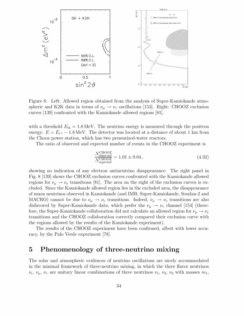
Analysis A

10-4

10-3

10-2

10-1

1

0 0.1 0.2 0.3 0.4 0.5 0.6 0.7 0.8 0.9 1sin2(2θ)

δm2 (

eV2 )

90% CL Kamiokande (multi-GeV)

90% CL Kamiokande (sub+multi-GeV)

νe → νx

90% CL

95% CL

Figure 8: Left: Allowed region obtained from the analysis of Super-Kamiokande atmo-spheric and K2K data in terms of νµ → ντ oscillations [153]. Right: CHOOZ exclusioncurves [139] confronted with the Kamiokande allowed regions [81].

with a threshold Eth = 1.8 MeV. The neutrino energy is measured through the positronenergy: E = Ee+ − 1.8 MeV. The detector was located at a distance of about 1 km fromthe Chooz power station, which has two pressurized-water reactors.

The ratio of observed and expected number of events in the CHOOZ experiment is

NCHOOZobserved

NCHOOZexpected

= 1.01 ± 0.04 , (4.32)

showing no indication of any electron antineutrino disappearance. The right panel inFig. 8 [139] shows the CHOOZ exclusion curves confronted with the Kamiokande allowedregions for νµ → νe transitions [81]. The area on the right of the exclusion curves is ex-cluded. Since the Kamiokande allowed region lies in the excluded area, the disappearanceof muon neutrinos observed in Kamiokande (and IMB, Super-Kamiokande, Soudan-2 andMACRO) cannot be due to νµ → νe transitions. Indeed, νµ → νe transitions are alsodisfavored by Super-Kamiokande data, which prefer the νµ → ντ channel [154] (there-fore, the Super-Kamiokande collaboration did not calculate an allowed region for νµ → νe

transitions and the CHOOZ collaboration correctly compared their exclusion curve withthe regions allowed by the results of the Kamiokande experiment).

The results of the CHOOZ experiment have been confirmed, albeit with lower accu-racy, by the Palo Verde experiment [78].

5 Phenomenology of three-neutrino mixing

The solar and atmospheric evidences of neutrino oscillations are nicely accommodatedin the minimal framework of three-neutrino mixing, in which the three flavor neutrinosνe, νµ, ντ are unitary linear combinations of three neutrinos ν1, ν2, ν3 with masses m1,

34

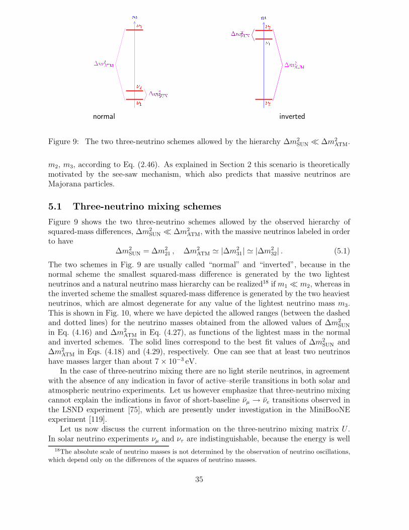
m2ATM

m

m2SUN21

3 m

3m2ATM

m2SUN 12

normal inverted

Figure 9: The two three-neutrino schemes allowed by the hierarchy ∆m2SUN ≪ ∆m2

ATM.

m2, m3, according to Eq. (2.46). As explained in Section 2 this scenario is theoreticallymotivated by the see-saw mechanism, which also predicts that massive neutrinos areMajorana particles.

5.1 Three-neutrino mixing schemes

Figure 9 shows the two three-neutrino schemes allowed by the observed hierarchy ofsquared-mass differences, ∆m2

SUN ≪ ∆m2ATM, with the massive neutrinos labeled in order

to have∆m2

SUN = ∆m221 , ∆m2

ATM ≃ |∆m231| ≃ |∆m2

32| . (5.1)

The two schemes in Fig. 9 are usually called “normal” and “inverted”, because in thenormal scheme the smallest squared-mass difference is generated by the two lightestneutrinos and a natural neutrino mass hierarchy can be realized18 if m1 ≪ m2, whereas inthe inverted scheme the smallest squared-mass difference is generated by the two heaviestneutrinos, which are almost degenerate for any value of the lightest neutrino mass m3.This is shown in Fig. 10, where we have depicted the allowed ranges (between the dashedand dotted lines) for the neutrino masses obtained from the allowed values of ∆m2

SUN

in Eq. (4.16) and ∆m2ATM in Eq. (4.27), as functions of the lightest mass in the normal

and inverted schemes. The solid lines correspond to the best fit values of ∆m2SUN and

∆m2ATM in Eqs. (4.18) and (4.29), respectively. One can see that at least two neutrinos

have masses larger than about 7 × 10−3 eV.In the case of three-neutrino mixing there are no light sterile neutrinos, in agreement

with the absence of any indication in favor of active–sterile transitions in both solar andatmospheric neutrino experiments. Let us however emphasize that three-neutrino mixingcannot explain the indications in favor of short-baseline νµ → νe transitions observed inthe LSND experiment [75], which are presently under investigation in the MiniBooNEexperiment [119].

Let us now discuss the current information on the three-neutrino mixing matrix U .In solar neutrino experiments νµ and ντ are indistinguishable, because the energy is well

18The absolute scale of neutrino masses is not determined by the observation of neutrino oscillations,which depend only on the differences of the squares of neutrino masses.

35

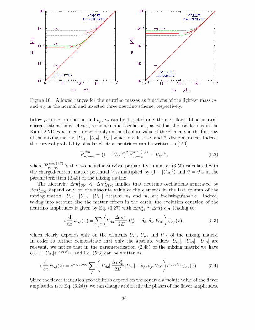
m3m2m1

m1 [eV m[eV

100101102103104

100101102103104 HIERARCHY

ALMOSTDEGENERATE m1, m2m3

m3 [eV m[eV

100101102103104

100101102103104 INVERTEDHIERARCHY

ALMOSTDEGENERATE

Figure 10: Allowed ranges for the neutrino masses as functions of the lightest mass m1

and m3 in the normal and inverted three-neutrino scheme, respectively.

below µ and τ production and νµ, ντ can be detected only through flavor-blind neutral-current interactions. Hence, solar neutrino oscillations, as well as the oscillations in theKamLAND experiment, depend only on the absolute value of the elements in the first rowof the mixing matrix, |Ue1|, |Ue2|, |Ue3| which regulates νe and νe disappearance. Indeed,the survival probability of solar electron neutrinos can be written as [159]

Psun

νe→νe=(1 − |Ue3|2

)2P

sun, (1,2)

νe→νe+ |Ue3|4 , (5.2)

where Psun, (1,2)

νe→νeis the two-neutrino survival probability in matter (3.50) calculated with

the charged-current matter potential VCC multiplied by (1 − |Ue3|2) and ϑ = ϑ12 in theparameterization (2.48) of the mixing matrix.

The hierarchy ∆m2SUN ≪ ∆m2

ATM implies that neutrino oscillations generated by∆m2

ATM depend only on the absolute value of the elements in the last column of themixing matrix, |Ue3|, |Uµ3|, |Uτ3| because m1 and m2 are indistinguishable. Indeed,taking into account also the matter effects in the earth, the evolution equation of theneutrino amplitudes is given by Eq. (3.27) with ∆m2

k1 ≃ ∆m231δk3, leading to

id

dxψαβ(x) =

∑

ρ

(Uβ3

∆m231

2EU∗

ρ3 + δβe δρe VCC

)ψαρ(x) , (5.3)

which clearly depends only on the elements Ue3, Uµ3 and Uτ3 of the mixing matrix.In order to further demonstrate that only the absolute values |Ue3|, |Uµ3|, |Uτ3| arerelevant, we notice that in the parameterization (2.48) of the mixing matrix we haveUβ3 = |Uβ3|e−iϕ13δβe, and Eq. (5.3) can be written as

id

dxψαβ(x) = e−iϕ13δβe

∑

ρ

(|Uβ3|

∆m231

2E|Uρ3| + δβe δρe VCC

)eiϕ13δρe ψαρ(x) . (5.4)

Since the flavor transition probabilities depend on the squared absolute value of the flavoramplitudes (see Eq. (3.26)), we can change arbitrarily the phases of the flavor amplitudes.

36

Making the change of phase

ψαβ(x) → e−iϕ13δβe ψαβ(x) , (5.5)

we obtain the evolution equation

id

dxψαβ(x) =

∑

ρ

(|Uβ3|

∆m231

2E|Uρ3| + δβe δρe VCC

)ψαρ(x) , (5.6)

which depends19 only on |Ue3|, |Uµ3| and |Uτ3|.The only connection between solar and atmospheric oscillations is due to |Ue3|. There-

fore, any information on the value of |Ue3| is of crucial importance.The key experiment for the determination of |Ue3| has been the CHOOZ long-baseline

reactor νe disappearance experiment [157, 139, 77], which did not observe any disappear-ance at a distance of about 1 km from the reactor source (see Section 4.3). The negativeresult of the CHOOZ experiment, confirmed by the Palo Verde experiment [78], impliesthat the oscillations of electron neutrinos at the atmospheric scale are very small or evenzero. The CHOOZ bound on the effective mixing angle (see Refs. [160, 21])

sin2 2ϑCHOOZ = 4 |Ue3|2(1 − |Ue3|2

)(5.7)

implies that |Ue3| is small:|Ue3|2 < 5 × 10−2 , (5.8)

at 99.73% C.L. [161]. Therefore, solar and atmospheric neutrino oscillations are practi-cally decoupled [160] and the effective mixing angles in solar, atmospheric and CHOOZexperiments can be related to the elements of the three-neutrino mixing matrix by (seealso Ref. [162])

sin2 ϑSUN =|Ue2|2

1 − |Ue3|2, sin2 ϑATM = |Uµ3|2 , sin2 ϑCHOOZ = |Ue3|2 . (5.9)

Taking into account the best-fit values of ϑSUN and ϑATM in Eqs. (4.18) and (4.29),respectively, and

sin2 ϑbfCHOOZ = 0 , (5.10)

the best-fit value for the mixing matrix U is

Ubf ≃(

0.84 0.55 0.00−0.39 0.59 0.710.39 −0.59 0.71

). (5.11)

Using the 99.73% C.L. allowed ranges for ϑSUN, ϑATM and ϑCHOOZ given by Eqs. (4.17),(4.28) and (5.8), respectively, we have reconstructed the allowed ranges for the elementsof the mixing matrix:

|U | ≃(

0.76−0.88 0.47−0.62 0.00−0.220.09−0.62 0.29−0.79 0.55−0.850.11−0.62 0.32−0.80 0.51−0.83

). (5.12)

Such mixing matrix, with all elements large except Ue3, is called “bilarge”. It is verydifferent from the quark mixing matrix, in which mixing is very small. This difference

19A simpler way to obtain the same result is to adopt a parameterization of the mixing matrix inwhich the Dirac phase is associated with the mixing angle ϑ12, which does not contribute to the evolutionequation (5.3) (see Ref. [59]).

37

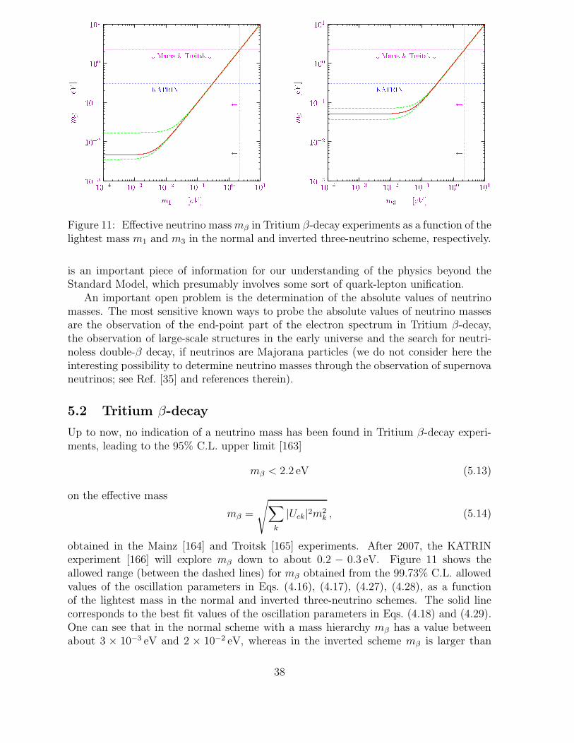
m1 [eV m [eV

101100101102103104

101100

101102103

# Mainz & Troitsk #

KATRIN

m3 [eV m [eV

101100101102103104

101100

101102103

# Mainz & Troitsk #

KATRIN

Figure 11: Effective neutrino massmβ in Tritium β-decay experiments as a function of thelightest mass m1 and m3 in the normal and inverted three-neutrino scheme, respectively.

is an important piece of information for our understanding of the physics beyond theStandard Model, which presumably involves some sort of quark-lepton unification.

An important open problem is the determination of the absolute values of neutrinomasses. The most sensitive known ways to probe the absolute values of neutrino massesare the observation of the end-point part of the electron spectrum in Tritium β-decay,the observation of large-scale structures in the early universe and the search for neutri-noless double-β decay, if neutrinos are Majorana particles (we do not consider here theinteresting possibility to determine neutrino masses through the observation of supernovaneutrinos; see Ref. [35] and references therein).

5.2 Tritium β-decay

Up to now, no indication of a neutrino mass has been found in Tritium β-decay experi-ments, leading to the 95% C.L. upper limit [163]

mβ < 2.2 eV (5.13)

on the effective mass

mβ =

√∑

k

|Uek|2m2k , (5.14)

obtained in the Mainz [164] and Troitsk [165] experiments. After 2007, the KATRINexperiment [166] will explore mβ down to about 0.2 − 0.3 eV. Figure 11 shows theallowed range (between the dashed lines) for mβ obtained from the 99.73% C.L. allowedvalues of the oscillation parameters in Eqs. (4.16), (4.17), (4.27), (4.28), as a functionof the lightest mass in the normal and inverted three-neutrino schemes. The solid linecorresponds to the best fit values of the oscillation parameters in Eqs. (4.18) and (4.29).One can see that in the normal scheme with a mass hierarchy mβ has a value betweenabout 3 × 10−3 eV and 2 × 10−2 eV, whereas in the inverted scheme mβ is larger than

38

about 3 × 10−2 eV. Therefore, if in the future it will be possible to constraint mβ to besmaller than about 3×10−2 eV, a normal hierarchy of neutrino masses will be established.

From Figs. 10 and 11 it is clear that the bound (5.13) can be saturated only if thethree neutrino masses are almost degenerate. In this case the dependence of mk on theindex k can be neglected in Eq. (5.14), leading to mβ ≃ mk. Therefore, the upper limitfor each mass is the same as the one on mβ in Eq. (5.13): at 95% C.L.

mk < 2.2 eV . (5.15)

5.3 Cosmological bounds on neutrino masses

In the early hot universe neutrinos are in equilibrium in the primeval plasma through the

weak interaction reactions νν e+e−,(−)

ν e (−)

ν e,(−)

ν N (−)

ν N , νen pe−, νep ne+,n pe−νe. As the universe expands and cools, the rate of weak interactions decreases.When the temperature of the Universe goes below T ≃ 1 MeV, the mean neutrino freepath becomes larger than the horizon20 and neutrinos practically cease to interact withthe plasma. At T . 0.5 MeV electron and positron in the plasma annihilate into photons,increasing the photon temperature Tγ with respect to the neutrino temperature Tν by afactor (11/4)1/3, easily calculated from entropy conservation (see Refs. [13, 14, 32]). Fromthe well measured temperature of the Cosmic Microwave Background Radiation (CMBR)Tγ = 2.725 ± 0.001 K, we infer the neutrino temperature Tν = 1.945 ± 0.001 K, andk Tν = 1.676±0.001×10−4 eV. As we have seen in Section 5.1, at least two neutrinos havemasses larger than about 7×10−3 eV (see Fig. 10). Hence, at least two massive neutrinosin the present relic neutrino background are non-relativistic. The number density ofrelic non-relativistic neutrinos can be calculated from the Fermi-Dirac distribution (seeRefs. [13, 14, 32]):

nνk,νk=

3

2

ζ(3)

π2T 3

ν ≃ 0.1827T 3ν ≃ 112 cm−3 , (5.16)

with ζ(3) ≃ 1.202. Their contribution to the present density of the universe (normalizedto the critical density ρc = 3H2/8πGN, where H is the Hubble constant and GN is theNewton constant) is given by

Ωk =nνk,νk

mk

ρc≃ 1

h2

mk

94.14 eV, (5.17)

where h is the value of the Hubble constant in units of 100 km s−1 Mpc−1 (the currentdetermination of h from a global fit of cosmological data is h = 0.71+0.04

−0.03 [167]). The totalcontribution of relic neutrinos to the present density of the universe is given by [168, 169]

Ων h2 =

∑k mk

94.14 eV. (5.18)

It is clear that, just from the need to avoid overclosing the Universe, the sum of neutrinomasses has to be lighter than about 100 eV. If one further takes h . 0.8 and Ων . 0.1,

20The horizon is the distance traveled by light from the beginning of the universe.

39

as indicated by astronomical data, one gets a quite restrictive upper bound of about 6eV for the sum of neutrino masses.

An even stronger bound on the sum of neutrino masses follows from more sophisticatedcalculations of structure formation in the early universe. Neutrinos with masses of theorder of 1 eV or lighter constitute what is called “hot dark matter”, which is dark matterthat is now non-relativistic, but was relativistic at the time of matter-radiation equality,when the contribution of matter and radiation to the density of the universe was equal.Since the radiation energy density scales as T 4 and matter energy density scale as T 3,matter started to dominate the density of the universe and structures started to formafter matter-radiation equality. However, hot dark matter particles did not participateto the beginning of structure formation at matter-radiation equality, but streamed freelyuntil they become non relativistic. Hence, neutrinos contribute only to the formation ofstructures with size given by the free-streaming distance traveled by neutrinos until theybecome non relativistic. The formation of structures on smaller scales is suppressed withrespect to a universe without hot dark matter. The absence of such suppression in thepresent astronomical observations of large scale structures (LSS) in the universe allow toput a strong upper bound on the sum of neutrino masses (see Refs. [170, 171, 172]).

The recent high-precision CMBR data of the WMAP satellite [173] combined withthe LSS data of the 2dF Galaxy Redshift Survey (2dFGRS) [174] and other astronomicaldata (see Ref. [167]) allowed the WMAP collaboration to derive the impressive bound

Ωνh2 < 0.0076 , (5.19)

with 95% confidence, which, using Eq. (5.18), yields∑

k

mk < 0.71 eV . (5.20)

From the smallness of the squared-mass differences implied by solar and atmosphericneutrino data (see Eqs. (4.16), (4.27) and (5.1)), it is clear that the bound (5.20) can besaturated only if the three neutrino masses are almost degenerate. Therefore, the upperlimit on each neutrino mass is one third of the bound in Eq.(5.20):

mk < 0.23 eV . (5.21)

This impressive limit is one order of magnitude more restrictive than the limit (5.15)obtained in Tritium experiments, reaching already the level of sensitivity of the futureKATRIN experiment. Let us emphasize, however, that the KATRIN experiment is im-portant in order to probe the neutrino masses in a model-independent way. Indeed,the cosmological bound relies on several assumptions on the cosmological model andsome controversial data (see the discussion in Ref. [175] and Ref. [176] for an alternativemodel). Using only the WMAP and 2dFGRS data, the author of Ref. [177] found the95% confidence limit ∑

k

mk < 2.12 eV . (5.22)

Adding also the Hubble Space Telescope determination of h, the authors of Ref. [178]obtained the 95% confidence limit

∑

k

mk < 1.1 eV . (5.23)

40

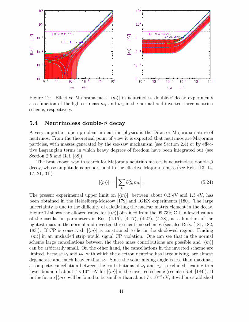
m1 [eV jhmij[eV

101100101102103104

101100101102103104 m1 [eV jhmij[eV

101100101102103104

101100101102103104

# H-M & IGEX #CP violation !

m3 [eV jhmij[eV

101100101102103104

101100101102103104 m3 [eV jhmij[eV

101100101102103104

101100101102103104

# H-M & IGEX #CP violation !

Figure 12: Effective Majorana mass |〈m〉| in neutrinoless double-β decay experimentsas a function of the lightest mass m1 and m3 in the normal and inverted three-neutrinoscheme, respectively.

5.4 Neutrinoless double-β decay

A very important open problem in neutrino physics is the Dirac or Majorana nature ofneutrinos. From the theoretical point of view it is expected that neutrinos are Majoranaparticles, with masses generated by the see-saw mechanism (see Section 2.4) or by effec-tive Lagrangian terms in which heavy degrees of freedom have been integrated out (seeSection 2.5 and Ref. [38]).

The best known way to search for Majorana neutrino masses is neutrinoless double-βdecay, whose amplitude is proportional to the effective Majorana mass (see Refs. [13, 14,17, 21, 31])

|〈m〉| =

∣∣∣∣∑

k

U2ek mk

∣∣∣∣ . (5.24)

The present experimental upper limit on |〈m〉|, between about 0.3 eV and 1.3 eV, hasbeen obtained in the Heidelberg-Moscow [179] and IGEX experiments [180]. The largeuncertainty is due to the difficulty of calculating the nuclear matrix element in the decay.Figure 12 shows the allowed range for |〈m〉| obtained from the 99.73% C.L. allowed valuesof the oscillation parameters in Eqs. (4.16), (4.17), (4.27), (4.28), as a function of thelightest mass in the normal and inverted three-neutrino schemes (see also Refs. [181, 182,183]). If CP is conserved, |〈m〉| is constrained to lie in the shadowed region. Finding|〈m〉| in an unshaded strip would signal CP violation. One can see that in the normalscheme large cancellations between the three mass contributions are possible and |〈m〉|can be arbitrarily small. On the other hand, the cancellations in the inverted scheme arelimited, because ν1 and ν2, with which the electron neutrino has large mixing, are almostdegenerate and much heavier than ν3. Since the solar mixing angle is less than maximal,a complete cancellation between the contributions of ν1 and ν2 is excluded, leading to alower bound of about 7×10−3 eV for |〈m〉| in the inverted scheme (see also Ref. [184]). Ifin the future |〈m〉| will be found to be smaller than about 7×10−3 eV, it will be established

41

that either neutrinos have a mass hierarchy or they are Dirac particles. Many neutrinolessdouble-β decay experiments are planned for the future (see Refs. [185, 35, 186, 187]). Themost sensitive may be able to probe such small values of |〈m〉|.

6 Future prospects

As reviewed in Section 4, in recent years neutrino oscillations have been established in amodel-independent way in solar (∼ 19σ) and atmospheric (∼ 7σ) neutrino experiments.An impressive proof of neutrino oscillations has also been obtained in the KamLAND re-actor experiment (∼ 4σ). As we have discussed in Section 5, all these experimental resultsare nicely accommodated in the framework of three-neutrino mixing. Only the LSNDanomaly [75] does not fit in this scheme, as already noticed. Its interpretation in terms ofneutrino oscillation is presently under investigation in the MiniBooNE experiment [119].

Putting aside for the moment the controversial LSND anomaly, the immediate fu-ture prospects of neutrino oscillation research deal with the precise determination of theparameters of the three-neutrino mixing matrix. The actual value of |Ue3|, the real un-known, will be searched for in the near future with the long baseline accelerator neutrinoprograms MINOS [79, 188] in the United States, OPERA [189] and ICARUS [190] inEurope (CERN to Gran Sasso [80]) and JHF [191] in Japan. All these projects useconventional neutrino beams.

However, the evolution of neutrino physics demands new schemes to produce intense,collimated and pure neutrino beams. New possibilities have been studied in the last fewyears: neutrino beams from a Neutrino Factory, Beta-Beams and Super-Beams, that herewe briefly summarize.

The current Neutrino Factory concept implies the production, collection, and storageof muons to produce very intense beams of muon and electron neutrinos with equalfluxes through the decays (4.21). Research and development addressing the feasibilityof a Neutrino Factory are currently in progress. Review studies on the physics reach ofthe Neutrino Factory option are given in Refs. [192, 193]. Incidentally, we notice thatanomalous muon decays, due to non standard weak interactions, if responsible of theobserved LSND effect, could be easily tested at a Neutrino Factory with a short-baselineexperiment, using a 10 ton detector capable of charge discrimination [125].

The Beta-Beam concept, first proposed in Ref. [194], is based on the accelerationand storage of radioactive ions. The β-decay of these radioactive ions can produce avery intense beam of electron neutrinos or antineutrinos with perfectly known energyspectrum. The physics reach of a CERN based Beta-Beam and of a Super-Beam+Beta-Beam combination is studied in Ref. [195]. In this study a Super-Beam is a very intenseνµ beam that has a Super Proton Linac (SPL) as injector delivering 1023 protons ontarget per year with energy of 2.2 GeV (see also Ref. [196]). The sensitivity to theDirac CP-violating phase ϕ13 in the neutrino mixing matrix (2.48) reachable in a Super-Beam+Beta-Beam combination results to be comparable to the sensitivity reachable ina Neutrino Factory if sin2 ϑ13 & 10−4. Comparisons between the sensitivities of differentprojects already approved or planned are presented in Ref. [197].

A next-generation neutrino oscillation experiment using reactor antineutrinos couldgive important information on the size of the mixing angle ϑ13 [198, 200]. Reactor exper-

42

iments can give a clean measure of the mixing angle without ambiguities associated withthe size of the other mixing angles, matter effects, and effects due to CP violation. Thekey question is whether a next-generation experiment can reach the needed sensitivitygoals to make a measurement of sin2 2ϑ13 at the 10−2 level [199, 200].

However, the search for |U13| and CP violation in the lepton sector does not coverall the items in today neutrino physics. Let us emphasize that still several fundamentalcharacteristics of neutrinos are unknown. Among them, the Dirac or Majorana nature ofneutrinos, the absolute scale of neutrino masses, the distinction between the normal andinverted schemes and the electromagnetic properties of neutrinos.

In our opinion the most important question in today neutrino physics is: are massiveneutrinos Majorana particles? This question can be resolved with an affirmative answerif neutrinoless beta decay is observed [201, 202]. Many experimental proposals existthat will increase dramatically the sensitivity of the neutrinoless double-β decay search,reaching |〈m〉| ∼ 10−2 eV (see Refs. [185, 35, 186, 187]).

Besides masses, neutrinos can have magnetic moments (see Refs. [17, 13, 14, 36]). Inthe case of a Dirac neutrino, a large enough magnetic moment could lead to spin preces-sion in a transverse magnetic field [203, 204, 205, 206], generating transitions between aneutrino with negative helicity and one with positive helicity, which is practically sterile.A Majorana neutrino cannot have a magnetic moment, but different Majorana neutri-nos can have transition magnetic moments, which could lead to Spin-Flavor Precession(SFP). However, SFP is suppressed in vacuum by the mass difference of different neu-trinos. In 1988 Akhmedov [207, 208] and Lim and Marciano [209] discovered that themass difference can be compensated by the matter potential for neutrinos propagating ina medium, leading to the so-called Resonant Spin-Flavor Precession (RSFP) mechanism,which is analogous to the MSW effect.

The RSFP mechanism was proposed as a possible explanation of the solar neutrinoproblem and was considered a viable possibility for many years. Now we know that thesolar neutrino problem is due to neutrino oscillations (see Section 4.1), but RSFP couldstill be a subdominant mechanism (see Ref. [210]). A possible signature of RSFP would bea periodic variability of the solar neutrino flux due to temporal variations of the magneticfield or to the inclination of the solar equator with respect to the ecliptic. A recent analysisof Super-Kamiokande data put severe limits to possible periodic modulations of the 8Bsolar neutrino flux [211] (see, however, Ref. [212] for a different point of view).

If massive neutrinos are Majorana particles, a combination of the RSFP mechanismand oscillations can induce besides νe → νµ, ντ , νµ, ντ transitions also νe → νe transitions21

of solar neutrinos [213, 214, 215], which can be observed in solar neutrino detectorsthrough the inverse β-decay process (4.31). However, the Super-Kamiokande experimentdid not find any indication of νe’s coming from the sun and established an upper limitof 8 × 10−3 for the averaged probability of νe → νe conversion in the energy range 8-20MeV (assuming the initial Standard Solar Model 8B νe flux) [216].

In any case, even if at the moment there seems to be no indication of an effect of theRSFP mechanism in solar neutrino data, it is important to pursue this line of research,because magnetic moments are important properties and the existence of large neutrinomagnetic moments could give crucial indications on the physics beyond the Standard

21Here νe is the conventional name for a neutrino state with almost exact positive helicity, which caninduce the creation of a positron upon scattering with matter (see the remark at the end of Section 2.6).

43

Model.Direct measurements of neutrino magnetic moments are also planned: a proposal on

the direct detection of antineutrino-electron scattering with an artificial tritium source[217] will search for a neutrino magnetic moment about two orders of magnitude smallerthan the present-day laboratory upper limit, reaching a sensitivity of about 10−12 µB,where µB is the Bohr magneton.

7 Conclusions

The recent years have been extraordinarily fruitful for neutrino physics, yielding model-independent proofs of solar and atmospheric neutrino oscillations, which have been con-firmed, respectively, by the reactor experiment KamLAND and the accelerator experi-ment K2K. Taking into account the negative result of the CHOOZ long-baseline reactorνe disappearance experiment, the global fit of solar, KamLAND, atmospheric and K2Kdata have provided important information on the neutrino mixing parameters in theframework of three-neutrino mixing, which is predicted by the natural versions of thesee-saw mechanism.

The only experimental result that cannot be explained in the framework of three-neutrino mixing is the controversial indication in favor of short-baseline νµ → νe tran-sitions observed in the LSND experiment. It is very important that the MiniBooNEexperiment running at Fermilab will check the validity of the LSND indication in thenear future. If MiniBooNE will obtain a positive result, the investigation of new possibil-ities (as four-neutrino mixing, CPT violation, etc.) will become imperative. These newphenomena would be very interesting for our understanding of the physics beyond theStandard Model.

Even if the values of some parameters of three-neutrino mixing are determined with aprecision that was unthinkable a few years ago, still several fundamental characteristics ofneutrinos remain unknown. Among them the most important are: the Dirac or Majorananature of neutrinos, the absolute scale of neutrino masses, the distinction between thenormal and inverted schemes, the value of |Ue3|, the existence of CP violation in the leptonsector, the number of light neutrinos and the electromagnetic properties of neutrinos.Several existing experiments and future projects are aimed at the exploration of thesecharacteristics, which are very important for our understanding of neutrino physics. Theirdetermination is likely to shed some light on the new physics beyond the Standard Model.Therefore, we think that interesting years lie ahead in neutrino physics research.

References

[1] B. Pontecorvo, Sov. Phys. JETP 6 (1957) 429 [Zh. Eksp. Teor. Fiz. 33 (1957) 549].

[2] B. Pontecorvo, Sov. Phys. JETP 7 (1958) 172 [Zh. Eksp. Teor. Fiz. 34 (1958) 247].

[3] Super-Kamiokande, Y. Fukuda et al., Phys. Rev. Lett. 81 (1998) 1562,hep-ex/9807003.

[4] Kamiokande-II, K.S. Hirata et al., Phys. Lett. B205 (1988) 416.

44

[5] IMB, R.M. Bionta et al., Phys. Rev. D38 (1988) 768.

[6] K2K, M.H. Ahn et al., Phys. Rev. Lett. 90 (2003) 041801, hep-ex/0212007.

[7] SNO, Q.R. Ahmad et al., Phys. Rev. Lett. 87 (2001) 071301, nucl-ex/0106015.

[8] Super-Kamiokande, S. Fukuda et al., Phys. Rev. Lett. 86 (2001) 5651,hep-ex/0103032.

[9] Homestake, B.T. Cleveland et al., Astrophys. J. 496 (1998) 505.

[10] SNO, Q.R. Ahmad et al., Phys. Rev. Lett. 89 (2002) 011301, nucl-ex/0204008.

[11] SNO, S. Ahmed et al., nucl-ex/0309004.

[12] KamLAND, K. Eguchi et al., Phys. Rev. Lett. 90 (2003) 021802, hep-ex/0212021.

[13] R.N. Mohapatra and P.B. Pal, Massive neutrinos in physics and astrophysics (WorldSci. Lect. Notes Phys. 60, 1998).

[14] C.W. Kim and A. Pevsner, Neutrinos in physics and astrophysics (Harwood Aca-demic Press, Chur, Switzerland, 1993), Contemporary Concepts in Physics, Vol.8.

[15] J.N. Bahcall, Neutrino Astrophysics (Cambridge University Press, 1989).

[16] S.M. Bilenky and B. Pontecorvo, Phys. Rept. 41 (1978) 225.

[17] S.M. Bilenky and S.T. Petcov, Rev. Mod. Phys. 59 (1987) 671.

[18] S.P. Mikheev and A.Y. Smirnov, Sov. Phys. Usp. 30 (1987) 759.

[19] T.K. Kuo and J. Pantaleone, Rev. Mod. Phys. 61 (1989) 937.

[20] V. Castellani et al., Phys. Rept. 281 (1997) 309, astro-ph/9606180.

[21] S.M. Bilenky, C. Giunti and W. Grimus, Prog. Part. Nucl. Phys. 43 (1999) 1,hep-ph/9812360.

[22] G. Altarelli and F. Feruglio, Phys. Rept. 320 (1999) 295, hep-ph/9905536.

[23] T. Kajita and Y. Totsuka, Rev. Mod. Phys. 73 (2001) 85.

[24] C.K. Jung et al., Ann. Rev. Nucl. Part. Sci. 51 (2001) 451.

[25] M.F. Altmann, R.L. Mossbauer and L.J.N. Oberauer, Rept. Prog. Phys. 64 (2001)97.

[26] S.M. Bilenky and C. Giunti, Int. J. Mod. Phys. A16 (2001) 3931, hep-ph/0102320.

[27] M. Beuthe, Phys. Rept. 375 (2003) 105, hep-ph/0109119.

[28] T.K. Gaisser and M. Honda, Ann. Rev. Nucl. Part. Sci. 52 (2002) 153,hep-ph/0203272.

45

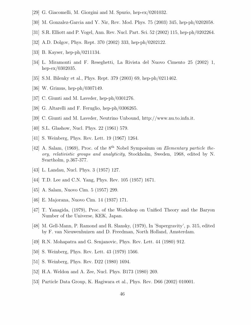
[29] G. Giacomelli, M. Giorgini and M. Spurio, hep-ex/0201032.

[30] M. Gonzalez-Garcia and Y. Nir, Rev. Mod. Phys. 75 (2003) 345, hep-ph/0202058.

[31] S.R. Elliott and P. Vogel, Ann. Rev. Nucl. Part. Sci. 52 (2002) 115, hep-ph/0202264.

[32] A.D. Dolgov, Phys. Rept. 370 (2002) 333, hep-ph/0202122.

[33] B. Kayser, hep-ph/0211134.

[34] L. Miramonti and F. Reseghetti, La Rivista del Nuovo Cimento 25 (2002) 1,hep-ex/0302035.

[35] S.M. Bilenky et al., Phys. Rept. 379 (2003) 69, hep-ph/0211462.

[36] W. Grimus, hep-ph/0307149.

[37] C. Giunti and M. Laveder, hep-ph/0301276.

[38] G. Altarelli and F. Feruglio, hep-ph/0306265.

[39] C. Giunti and M. Laveder, Neutrino Unbound, http://www.nu.to.infn.it.

[40] S.L. Glashow, Nucl. Phys. 22 (1961) 579.

[41] S. Weinberg, Phys. Rev. Lett. 19 (1967) 1264.

[42] A. Salam, (1969), Proc. of the 8th Nobel Symposium on Elementary particle the-

ory, relativistic groups and analyticity, Stockholm, Sweden, 1968, edited by N.Svartholm, p.367-377.

[43] L. Landau, Nucl. Phys. 3 (1957) 127.

[44] T.D. Lee and C.N. Yang, Phys. Rev. 105 (1957) 1671.

[45] A. Salam, Nuovo Cim. 5 (1957) 299.

[46] E. Majorana, Nuovo Cim. 14 (1937) 171.

[47] T. Yanagida, (1979), Proc. of the Workshop on Unified Theory and the BaryonNumber of the Universe, KEK, Japan.

[48] M. Gell-Mann, P. Ramond and R. Slansky, (1979), In ’Supergravity’, p. 315, editedby F. van Nieuwenhuizen and D. Freedman, North Holland, Amsterdam.

[49] R.N. Mohapatra and G. Senjanovic, Phys. Rev. Lett. 44 (1980) 912.

[50] S. Weinberg, Phys. Rev. Lett. 43 (1979) 1566.

[51] S. Weinberg, Phys. Rev. D22 (1980) 1694.

[52] H.A. Weldon and A. Zee, Nucl. Phys. B173 (1980) 269.

[53] Particle Data Group, K. Hagiwara et al., Phys. Rev. D66 (2002) 010001.

46

[54] S.S. Bulanov et al., hep-ph/0301268.

[55] K. Belotsky et al., Phys. Rev. D68 (2003) 054027, hep-ph/0210153.

[56] F.D. Murnaghan, The unitary and rotation groups (Spartan Articles, WashingtonD.C., 1962).

[57] J. Schechter and J.W.F. Valle, Phys. Rev. D21 (1980) 309.

[58] J. Schechter and J.W.F. Valle, Phys. Rev. D22 (1980) 2227.

[59] C. Giunti, C.W. Kim and M. Monteno, Nucl. Phys. B521 (1998) 3, hep-ph/9709439.

[60] C. Giunti and M. Tanimoto, Phys. Rev. D66 (2002) 113006, hep-ph/0209169.

[61] GALLEX, W. Hampel et al., Phys. Lett. B447 (1999) 127.

[62] SAGE, J.N. Abdurashitov et al., J. Exp. Theor. Phys. 95 (2002) 181,astro-ph/0204245.

[63] GNO, M. Altmann et al., Phys. Lett. B490 (2000) 16, hep-ex/0006034.

[64] Bugey, Y. Declais et al., Nucl. Phys. B434 (1995) 503.

[65] CHOOZ, M. Apollonio et al., Phys. Lett. B466 (1999) 415, hep-ex/9907037.

[66] Super-Kamiokande, S. Fukuda et al., Phys. Lett. B539 (2002) 179, hep-ex/0205075.

[67] Super-Kamiokande, M. Smy et al., hep-ex/0309011.

[68] C. Giunti, C.W. Kim and U.W. Lee, Phys. Rev. D45 (1992) 2414.

[69] C. Giunti and C.W. Kim, Found. Phys. Lett. 14 (2001) 213, hep-ph/0011074.

[70] C. Giunti, hep-ph/0302026.

[71] CDHS, F. Dydak et al., Phys. Lett. B134 (1984) 281.

[72] CCFR/NuTeV, D. Naples et al., Phys. Rev. D59 (1999) 031101, hep-ex/9809023.

[73] CHORUS, E. Eskut et al., Phys. Lett. B497 (2001) 8.

[74] NOMAD, P. Astier et al., Phys. Lett. B570 (2003) 19, hep-ex/0306037.

[75] LSND, A. Aguilar et al., Phys. Rev. D64 (2001) 112007, hep-ex/0104049.

[76] KARMEN, B. Armbruster et al., Phys. Rev. D65 (2002) 112001, hep-ex/0203021.

[77] CHOOZ, M. Apollonio et al., Eur. Phys. J. C27 (2003) 331, hep-ex/0301017.

[78] Palo Verde, F. Boehm et al., Phys. Rev. D64 (2001) 112001, hep-ex/0107009.

[79] MINOS, M.V. Diwan, eConf C0209101 (2002) TH08, hep-ex/0211026.

[80] D. Duchesneau, eConf C0209101 (2002) TH09, hep-ex/0209082.

47

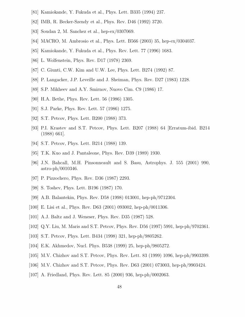
[81] Kamiokande, Y. Fukuda et al., Phys. Lett. B335 (1994) 237.

[82] IMB, R. Becker-Szendy et al., Phys. Rev. D46 (1992) 3720.

[83] Soudan 2, M. Sanchez et al., hep-ex/0307069.

[84] MACRO, M. Ambrosio et al., Phys. Lett. B566 (2003) 35, hep-ex/0304037.

[85] Kamiokande, Y. Fukuda et al., Phys. Rev. Lett. 77 (1996) 1683.

[86] L. Wolfenstein, Phys. Rev. D17 (1978) 2369.

[87] C. Giunti, C.W. Kim and U.W. Lee, Phys. Lett. B274 (1992) 87.

[88] P. Langacker, J.P. Leveille and J. Sheiman, Phys. Rev. D27 (1983) 1228.

[89] S.P. Mikheev and A.Y. Smirnov, Nuovo Cim. C9 (1986) 17.

[90] H.A. Bethe, Phys. Rev. Lett. 56 (1986) 1305.

[91] S.J. Parke, Phys. Rev. Lett. 57 (1986) 1275.

[92] S.T. Petcov, Phys. Lett. B200 (1988) 373.

[93] P.I. Krastev and S.T. Petcov, Phys. Lett. B207 (1988) 64 [Erratum-ibid. B214(1988) 661].

[94] S.T. Petcov, Phys. Lett. B214 (1988) 139.

[95] T.K. Kuo and J. Pantaleone, Phys. Rev. D39 (1989) 1930.

[96] J.N. Bahcall, M.H. Pinsonneault and S. Basu, Astrophys. J. 555 (2001) 990,astro-ph/0010346.

[97] P. Pizzochero, Phys. Rev. D36 (1987) 2293.

[98] S. Toshev, Phys. Lett. B196 (1987) 170.

[99] A.B. Balantekin, Phys. Rev. D58 (1998) 013001, hep-ph/9712304.

[100] E. Lisi et al., Phys. Rev. D63 (2001) 093002, hep-ph/0011306.

[101] A.J. Baltz and J. Weneser, Phys. Rev. D35 (1987) 528.

[102] Q.Y. Liu, M. Maris and S.T. Petcov, Phys. Rev. D56 (1997) 5991, hep-ph/9702361.

[103] S.T. Petcov, Phys. Lett. B434 (1998) 321, hep-ph/9805262.

[104] E.K. Akhmedov, Nucl. Phys. B538 (1999) 25, hep-ph/9805272.

[105] M.V. Chizhov and S.T. Petcov, Phys. Rev. Lett. 83 (1999) 1096, hep-ph/9903399.

[106] M.V. Chizhov and S.T. Petcov, Phys. Rev. D63 (2001) 073003, hep-ph/9903424.

[107] A. Friedland, Phys. Rev. Lett. 85 (2000) 936, hep-ph/0002063.

48

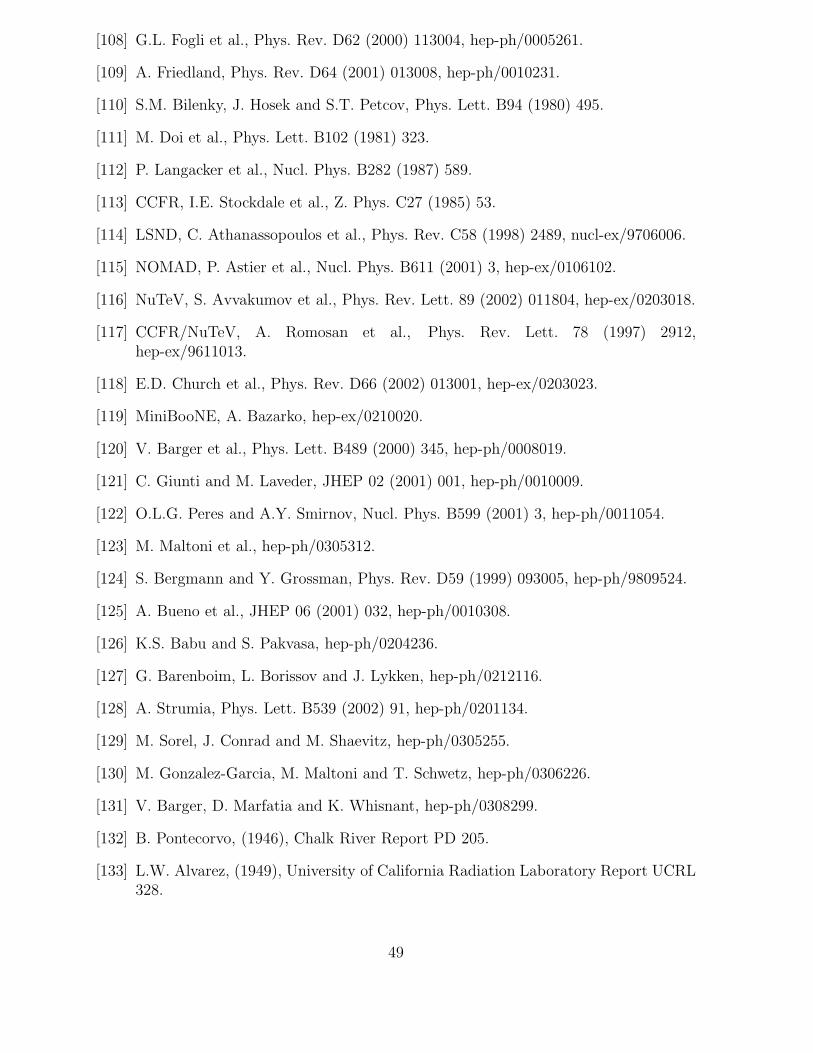
[108] G.L. Fogli et al., Phys. Rev. D62 (2000) 113004, hep-ph/0005261.

[109] A. Friedland, Phys. Rev. D64 (2001) 013008, hep-ph/0010231.

[110] S.M. Bilenky, J. Hosek and S.T. Petcov, Phys. Lett. B94 (1980) 495.

[111] M. Doi et al., Phys. Lett. B102 (1981) 323.

[112] P. Langacker et al., Nucl. Phys. B282 (1987) 589.

[113] CCFR, I.E. Stockdale et al., Z. Phys. C27 (1985) 53.

[114] LSND, C. Athanassopoulos et al., Phys. Rev. C58 (1998) 2489, nucl-ex/9706006.

[115] NOMAD, P. Astier et al., Nucl. Phys. B611 (2001) 3, hep-ex/0106102.

[116] NuTeV, S. Avvakumov et al., Phys. Rev. Lett. 89 (2002) 011804, hep-ex/0203018.

[117] CCFR/NuTeV, A. Romosan et al., Phys. Rev. Lett. 78 (1997) 2912,hep-ex/9611013.

[118] E.D. Church et al., Phys. Rev. D66 (2002) 013001, hep-ex/0203023.

[119] MiniBooNE, A. Bazarko, hep-ex/0210020.

[120] V. Barger et al., Phys. Lett. B489 (2000) 345, hep-ph/0008019.

[121] C. Giunti and M. Laveder, JHEP 02 (2001) 001, hep-ph/0010009.

[122] O.L.G. Peres and A.Y. Smirnov, Nucl. Phys. B599 (2001) 3, hep-ph/0011054.

[123] M. Maltoni et al., hep-ph/0305312.

[124] S. Bergmann and Y. Grossman, Phys. Rev. D59 (1999) 093005, hep-ph/9809524.

[125] A. Bueno et al., JHEP 06 (2001) 032, hep-ph/0010308.

[126] K.S. Babu and S. Pakvasa, hep-ph/0204236.

[127] G. Barenboim, L. Borissov and J. Lykken, hep-ph/0212116.

[128] A. Strumia, Phys. Lett. B539 (2002) 91, hep-ph/0201134.

[129] M. Sorel, J. Conrad and M. Shaevitz, hep-ph/0305255.

[130] M. Gonzalez-Garcia, M. Maltoni and T. Schwetz, hep-ph/0306226.

[131] V. Barger, D. Marfatia and K. Whisnant, hep-ph/0308299.

[132] B. Pontecorvo, (1946), Chalk River Report PD 205.

[133] L.W. Alvarez, (1949), University of California Radiation Laboratory Report UCRL328.

49

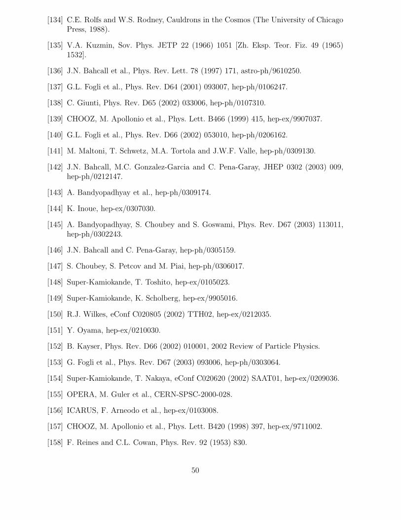
[134] C.E. Rolfs and W.S. Rodney, Cauldrons in the Cosmos (The University of ChicagoPress, 1988).

[135] V.A. Kuzmin, Sov. Phys. JETP 22 (1966) 1051 [Zh. Eksp. Teor. Fiz. 49 (1965)1532].

[136] J.N. Bahcall et al., Phys. Rev. Lett. 78 (1997) 171, astro-ph/9610250.

[137] G.L. Fogli et al., Phys. Rev. D64 (2001) 093007, hep-ph/0106247.

[138] C. Giunti, Phys. Rev. D65 (2002) 033006, hep-ph/0107310.

[139] CHOOZ, M. Apollonio et al., Phys. Lett. B466 (1999) 415, hep-ex/9907037.

[140] G.L. Fogli et al., Phys. Rev. D66 (2002) 053010, hep-ph/0206162.

[141] M. Maltoni, T. Schwetz, M.A. Tortola and J.W.F. Valle, hep-ph/0309130.

[142] J.N. Bahcall, M.C. Gonzalez-Garcia and C. Pena-Garay, JHEP 0302 (2003) 009,hep-ph/0212147.

[143] A. Bandyopadhyay et al., hep-ph/0309174.

[144] K. Inoue, hep-ex/0307030.

[145] A. Bandyopadhyay, S. Choubey and S. Goswami, Phys. Rev. D67 (2003) 113011,hep-ph/0302243.

[146] J.N. Bahcall and C. Pena-Garay, hep-ph/0305159.

[147] S. Choubey, S. Petcov and M. Piai, hep-ph/0306017.

[148] Super-Kamiokande, T. Toshito, hep-ex/0105023.

[149] Super-Kamiokande, K. Scholberg, hep-ex/9905016.

[150] R.J. Wilkes, eConf C020805 (2002) TTH02, hep-ex/0212035.

[151] Y. Oyama, hep-ex/0210030.

[152] B. Kayser, Phys. Rev. D66 (2002) 010001, 2002 Review of Particle Physics.

[153] G. Fogli et al., Phys. Rev. D67 (2003) 093006, hep-ph/0303064.

[154] Super-Kamiokande, T. Nakaya, eConf C020620 (2002) SAAT01, hep-ex/0209036.

[155] OPERA, M. Guler et al., CERN-SPSC-2000-028.

[156] ICARUS, F. Arneodo et al., hep-ex/0103008.

[157] CHOOZ, M. Apollonio et al., Phys. Lett. B420 (1998) 397, hep-ex/9711002.

[158] F. Reines and C.L. Cowan, Phys. Rev. 92 (1953) 830.

50

[159] X. Shi and D.N. Schramm, Phys. Lett. B283 (1992) 305.

[160] S.M. Bilenky and C. Giunti, Phys. Lett. B444 (1998) 379, hep-ph/9802201.

[161] G.L. Fogli et al., Phys. Rev. D66 (2002) 093008, hep-ph/0208026.

[162] W.L. Guo and Z.Z. Xing, Phys. Rev. D67 (2003) 053002, hep-ph/0212142.

[163] C. Weinheimer, hep-ex/0210050.

[164] Mainz, C. Weinheimer et al., Phys. Lett. B460 (1999) 219.

[165] Troitsk, V.M. Lobashev et al., Phys. Lett. B460 (1999) 227.

[166] KATRIN, A. Osipowicz et al., hep-ex/0109033.

[167] D.N. Spergel et al., astro-ph/0302209.

[168] S.S. Gershtein and Y.B. Zeldovich, JETP Lett. 4 (1966) 120, [Pisma Zh. Eksp.Teor. Fiz. 4 (1966) 174].

[169] R. Cowsik and J. McClelland, Phys. Rev. Lett. 29 (1972) 669.

[170] W. Hu, D.J. Eisenstein and M. Tegmark, Phys. Rev. Lett. 80 (1998) 5255,astro-ph/9712057.

[171] X. Wang, M. Tegmark and M. Zaldarriaga, astro-ph/0105091.

[172] S. Hannestad, Phys. Rev. D67 (2003) 085017, astro-ph/0211106.

[173] C.L. Bennett et al., astro-ph/0302207.

[174] M. Colless et al., astro-ph/0306581.

[175] S. Hannestad, astro-ph/0310133.

[176] A. Blanchard et al., astro-ph/0304237.

[177] S. Hannestad, JCAP 0305 (2003) 004, astro-ph/0303076.

[178] O. Elgaroy and O. Lahav, JCAP 04 (2003) 004, astro-ph/0303089.

[179] H.V. Klapdor-Kleingrothaus et al., Eur. Phys. J. A12 (2001) 147.

[180] IGEX, C.E. Aalseth et al., Phys. Rev. D65 (2002) 092007, hep-ex/0202026.

[181] S. Pascoli, S.T. Petcov and W. Rodejohann, Phys. Lett. B549 (2002) 177,hep-ph/0209059.

[182] S. Pascoli and S.T. Petcov, hep-ph/0310003.

[183] F.R. Joaquim, Phys. Rev. D68 (2003) 033019, hep-ph/0304276.

[184] H. Murayama and C. Pena-Garay, hep-ph/0309114.

51

[185] O. Cremonesi, hep-ex/0210007.

[186] Y. Zdesenko, Rev. Mod. Phys. 74 (2002) 663.

[187] G. Gratta, Talk presented at the XXI International Symposium on Lepton Photon2003, 11-16 August 2003, Fermi National Accelerator Laboratory, Batavia, IllinoisUSA.

[188] D. Ayres et al., hep-ex/0210005.

[189] M. Komatsu, P. Migliozzi and F. Terranova, J. Phys. G29 (2003) 443,hep-ph/0210043.

[190] A. Rubbia and P. Sala, JHEP 09 (2002) 004, hep-ph/0207084.

[191] Super-Kamiokande, Y. Itow, Talk presented at the 31st International Conferenceon High Energy Physics, ICHEP 02, Amsterdam, Holland, 24-31 July 2002.

[192] M. Apollonio et al., hep-ph/0210192.

[193] C. Albright et al., hep-ex/0008064.

[194] P. Zucchelli, hep-ex/0107006.

[195] M. Mezzetto, J. Phys. G29 (2003) 1771, hep-ex/0302007.

[196] A. Blondel et al., Nucl. Instrum. Meth. A503 (2001) 173.

[197] D. Harris, Talk presented at the XXI International Symposium on Lepton Photon2003, 11-16 August 2003, Fermi National Accelerator Laboratory, Batavia, IllinoisUSA.

[198] H. Minakata et al., hep-ph/0211111.

[199] P. Huber, M. Lindner, T. Schwetz and W. Winter, Nucl. Phys. B665 (2003) 487,hep-ph/0303232.

[200] M.H. Shaevitz and J.M. Link, hep-ex/0306031.

[201] J. Schechter and J.W.F. Valle, Phys. Rev. D25 (1982) 2951.

[202] E. Takasugi, Phys. Lett. B149 (1984) 372.

[203] A. Cisneros, Astrophys. Space Sci. 10 (1971) 87.

[204] M.B. Voloshin and M.I. Vysotsky, Sov. J. Nucl. Phys. 44 (1986) 544.

[205] L.B. Okun, M.B. Voloshin and M.I. Vysotsky, Sov. Phys. JETP 64 (1986) 446.

[206] L.B. Okun, M.B. Voloshin and M.I. Vysotsky, Sov. J. Nucl. Phys. 44 (1986) 440.

[207] E.K. Akhmedov, Sov. J. Nucl. Phys. 48 (1988) 382.

[208] E.K. Akhmedov, Phys. Lett. B213 (1988) 64.

52

[209] C.S. Lim and W.J. Marciano, Phys. Rev. D37 (1988) 1368.

[210] E.K. Akhmedov and J. Pulido, Phys. Lett. B553 (2003) 7, hep-ph/0209192.

[211] Super-Kamiokande, J. Yoo et al., hep-ex/0307070.

[212] D.O. Caldwell and P.A. Sturrock, hep-ph/0309191.

[213] E.K. Akhmedov, Sov. Phys. JETP 68 (1989) 690.

[214] E.K. Akhmedov, Phys. Lett. B255 (1991) 84.

[215] E.K. Akhmedov, S.T. Petcov and A.Y. Smirnov, Phys. Lett. B309 (1993) 95,hep-ph/9301247.

[216] Super-Kamiokande, Y. Gando et al., Phys. Rev. Lett. 90 (2003) 171302,hep-ex/0212067.

[217] B.S. Neganov et al., Phys. Atom. Nucl. 64 (2001) 1948, hep-ex/0105083.

53