SHORT COURSE IIThe Science of Large Data Sets: Spikes, Fields, and VoxelsOrganized by Uri Eden, PhD

Neuroscience 2013

Short Course IIThe Science of Large Data Sets: Spikes, Fields, and Voxels

Organized by Uri Eden, PhD

Please cite articles using the model:[AUTHOR’S LAST NAME, AUTHOR’S FIRST & MIDDLE INITIALS] (2013)

[CHAPTER TITLE] In: The Science of Large Data Sets: Spikes, Fields, and Voxels. (Eberwine J, ed) pp. [xx-xx]. Washington, DC: Society for Neuroscience.

All articles and their graphics are under the copyright of their respective authors.

Cover graphics and design © 2013 Society for Neuroscience.

TIME AGENDA TOPICS SPEAKER

8:00 – 8:30 a.m. CHECK-IN

8:30 – 8:40 a.m. Opening remarks Uri Eden, PhD Boston University

8:40 – 9:25 a.m. Towards the brainome: tools for understanding molecules, connectivity, activity, and behavior

Ed Boyden, PhD MIT

9:25 – 10:10 a.m. Analyzing neural spiking with point process models Emery Brown, MD, PhD MIT

10:10 – 10:25 a.m. MORNING BREAK

10:25 – 11:10 a.m. Examples of spike train analysis with generalized linear models Sridevi Sarma, PhD Johns Hopkins University

11:10 – 11:55 a.m. Analyzing fields and spikes: rhythms and coupling Mark Kramer, PhD Boston University

11:55 a.m. – 12:40 p.m. Assimilating dynamic models from neural field and imaging data Rosalyn Moran, PhD Virginia Tech

12:40 – 1:40 p.m. LUNCH: ROOM 25ABC

1:40 – 2:25 p.m. Overcoming challenges of MEG/EEG data analysis: insights from biophysics, anatomy, and physiology

Matti Hämäläinen, PhD MGH

2:25 – 3:10 p.m. Statistical considerations for the analysis of functional MRI data Jeanette Mumford, PhD The University of Texas at Austin

3:10 – 4:10 p.m. SUMMARY, DISCUSSION, BREAKOUT GUIDE

4:10 – 4:30 p.m. AFTERNOON BREAK

AFTERNOON BREAKOUT SESSIONS Participants select one discussion group at 4:30 p.m. and one at 5:30 p.m.

TIME THEME ROOM

4:30 – 5:30 p.m. BREAKOUT SESSIONS

GROUP 1 – Spike train analysis tutorial 23A

GROUP 2 – Field analysis tutorial 23B

GROUP 3 – Imaging data analysis tutorial 23C

5:30 – 6:30 p.m. REPEAT SESSIONS ABOVE. SELECT A SECOND DISCUSSION GROUP.

SHORT COURSE IIThe Science of Large Data Sets: Spikes, Fields, and Voxels

Organized by: Uri Eden, PhDFriday, November 8 8:30 a.m. – 6:30 p.m. | San Diego | The San Diego Convention Center | Room: 6CF

Table of Contents

Introduction . . . . . . . . . . . . . . . . . . . . . . . . . . . . . . . . . . . . . . . . . . . . . . . . . . . . . . . . . . . . . . . . . . . . . 7

Supplementary Case Report for a Generalized Linear Model Lecture Sridevi Sarma, PhD . . . . . . . . . . . . . . . . . . . . . . . . . . . . . . . . . . . . . . . . . . . . . . . . . . . . . . . 9

An Introduction to Field Analysis Techniques: The Power Spectrum and Coherence Mark A . Kramer, PhD . . . . . . . . . . . . . . . . . . . . . . . . . . . . . . . . . . . . . . . . . . . . . . . . . . . . 17

Dynamic Causal Models for Human Electrophysiology: EEG, MEG, and Local Field Potentials Rosalyn Moran, PhD . . . . . . . . . . . . . . . . . . . . . . . . . . . . . . . . . . . . . . . . . . . . . . . . . . . . . 25

Overcoming Challenges of MEG/EEG Data Analysis: Insights from Biophysics, Anatomy, and Physiology Matti S . Hämäläinen, PhD . . . . . . . . . . . . . . . . . . . . . . . . . . . . . . . . . . . . . . . . . . . . . . . . . 33

Considerations When Using Single-Trial Parameter Estimates in Representational Similarity Analyses Jeanette A . Mumford, PhD . . . . . . . . . . . . . . . . . . . . . . . . . . . . . . . . . . . . . . . . . . . . . . . . . 41

Introduction

Modern methods for imaging and recording brain activity allow us to collect massive amounts of data across a wide range of spatial and temporal scales. Researchers now routinely record spike trains from hundreds of neurons across multiple brain regions, continuous fields from numerous brain sites over days at a time, and imaging data containing hundreds of gigabytes of information. In order to make use of the exciting opportunities afforded by this explosion of data, it is imperative for researchers to understand and be able to apply principled statistical methods. These methods should take advantage of the structure present in diverse neural data sets.

A fundamental challenge for understanding brain function has always been that neural processing for even the simplest tasks requires the interaction of thousands to millions of neurons distributed across multiple brain regions. In the past, many studies had been limited to either mapping out simple input–output relationships for individual neurons or local fields or identifying activity patterns in imaging data associated with specific tasks. Now, answers to many of the most intriguing open questions about brain function are within our reach for the first time, thanks to improvements in recording technologies and new data collection efforts. For example, recent initiatives have focused on characterizing connections, both anatomical and statistical, among neurons, neural populations, and large brain regions.

This short course will provide an overview of classic and modern data analysis methods. We will cover general principles of signal processing and statistical data analysis methods, with a focus on three common classes of signals: spike trains, electromagnetic fields at multiple spatial scales, and functional MRI (fMRI) data. For each type of signal, we will discuss distinct features of the data, basic methods to describe and visualize associations within those data, and modeling approaches that allow us to make statistical inferences about neural function.

© 2013 Sarma

Department of Applied Mathematics and Statistics Boston University

Boston, Massachusetts

Institute for Computational Medicine Department of Biomedical Engineering

Johns Hopkins University Baltimore, Maryland

Supplementary Case Report for a Generalized Linear Model Lecture

Sridevi Sarma, PhD

11

© 2013 Sarma

Supplementary Case Report for a Generalized Linear Model Lecture

Introduction: Spiking Patterns in Parkinson’s Disease and in HealthThe placement of deep-brain stimulating electrodes in the subthalamic nucleus (STN) to treat Parkinson’s disease (PD) also allows the recording of single neuron spiking activity. Analyses of these unique data offer an important opportunity to better understand the pathophysiology of PD. However, despite the point-process nature of PD neural spiking activity, point-process methods are rarely used to analyze these recordings.

We developed a point-process representation of PD neural spiking activity using a generalized linear model (GLM) to describe long- and short-term temporal dependencies in the spiking activity of 28 STN neurons from seven PD patients, and 35 neurons from one healthy primate (surrogate control), recorded while the subjects executed a directed hand-movement task. We used the point-process model to characterize each neuron’s bursting, oscillatory, and directional tuning properties during key periods in the task trial. Relative to the control neurons, the PD neurons showed increased bursting, increased 10–30 Hz oscillations, and increased fluctuations in directional tuning. These features, which traditional methods failed to capture accurately, were efficiently summarized in a single model in the point-process analysis of each neuron. The point-process framework suggests a useful approach for developing quantitative neural correlates that may be related directly to the movement and behavioral disorders characteristic of PD.

The GLM lecture described how one can model neural responses to stimuli with a generalized notion of linear regression. This supplementary document shows a published case study (Sarma et al., 2010) on how GLMs can be used to both model neuronal spiking data in response to a motor behavioral stimulus and make inferences about spiking patterns from model parameters.

Behavioral taskOnce microelectrodes were placed in the STN, the subjects viewed a computer monitor and performed a behavioral task by moving a joystick with the contralateral hand. The joystick was mounted such that movements were in a horizontal orientation with the elbow flexed at approximately 45°. The behavioral task began with the presentation of a small central fixation point. After a 500 ms delay, four small gray targets appeared arrayed in a circular fashion around the fixation point (up, right, down, and left). After a 500–1,000 ms delay, a randomly

selected target turned green (target cue [TC]) to indicate where the subject was to move. Then, after another 500–1,000 ms delay, the central fixation point turned green (go cue [GC]), cueing the subject to move. At this point, the subject used the joystick to guide a cursor from the center of the monitor toward the green target. Once the target was reached, either a juice reward was given (in the primate case) or a tone sounded, indicating that the subject had successfully completed the task (human case) and the stimuli were erased. Subjects were required to return the joystick to the center position before the next trial started. A schematic representation of a single trial is shown in Figure 1.

Point-process model of STN dynamicsWe formulated a point-process model to relate the spiking propensity of each STN neuron to factors associated with movement direction and features of the neuron’s spiking history. We used the model parameters to analyze oscillations, bursting, and directional tuning modulations across the entire trial and to make comparisons between two subject groups. A point process is a series of 01 random events that occur in continuous time. For a neural spike train, the 1s are individual spike times and the 0s are the times at which no spikes occur. To define a point-process model of neural spiking activity, in this analysis we considered an observation interval (0, T] and let N(t) be the number of spikes counted in interval (0, t] for t ϵ (0, T]. A point-process model of a neural spike train can be completely characterized by its cumulative intensity function (CIF), λ(t|Ht), defined as follows:

λ(t│Ht)= limΔ→0 Pr(N(t+Δ) – N(t) = 1| Ht)/Δ (1)

where Ht denotes the history of spikes up to time t. It follows from equation (2) that the probability of a single spike in a small interval (t, t + Δ] is approximately

Pr(spike in (t, t + Δ] | Ht) = λ (t|Ht) Δ (2)

Figure 1. Schematic of a behavioral task trial. U, R, D, L = Up, Right, Down, Left.

12

NoTeS

© 2013 Sarma

(Details can be found in Snyder and Miller, 1991, and Cox and Isham, 2000.) When Δ is small, equation (2) approximates the spiking propensity at time t.

The CIF generalizes the rate function of a Poisson process to a rate function that is history dependent. Because the conditional intensity function completely characterizes a spike train, defining a model for the CIF defines a model for the spike train (Brown et al., 2003; Brown, 2005). For our analyses, we used the GLM to define our CIF models by expressing, for each neuron, the log of its CIF in terms of the neuron’s spike history and relevant movement covariates (Truccollo et al., 2005). The GLM is an extension of the multiple linear regression model in which the variable being predicted (in this case, spike times) need not be Gaussian (McCullagh and Nelder, 1989). GLM also provides an efficient computational scheme for estimating model parameters and a likelihood framework for conducting statistical inferences (Brown et al., 2003).

We expressed the CIF for each neuron as a function of movement direction, which corresponds to up, right, left, and down, and the neuron’s spiking history in the preceding 150 ms. Instead of estimating the CIF continuously throughout the entire trial, we estimated it over 350 ms time windows around key epochs and at discrete time intervals, each 1 ms in duration. Specifically, we estimated the CIF over 350 ms windows centered at the gray array (GA) onset, TC onset, GC onset, and movement (MV) onset. We do not label each CIF with the corresponding epoch going forward for a simpler read and express the CIF as follows:

λ (t|Ht, θ) = λS (t|θ) λH (t|Ht, θ) (3)

where λS (t|θ) describes the effect of the movement direction stimulus on the neural response and λH

(t|Ht, θ) describes the effect of spiking history on the neural response. θ is a parameter vector to be estimated from data. The units of λS (t|θ) are spikes per second, and λH (t|Ht, θ) is dimensionless. The idea to express the CIF as a product of a stimulus component and a temporal or spike history component was first suggested by Kass and Ventura (2001). This idea is appealing, as it allows one to assess how much each component contributes to the spiking propensity of the neuron. If spiking history is not a factor associated with neural response, then λH (t|Ht, θ) will be very close to 1 for all times, and equation (1) reduces to an inhomogeneous Poisson process.

The model of the stimulus effect is as follows:

λS (t|θ) = αdId (t), (4)

where d = 1, 2, 3, 4 is the movement direction, Id (t) = 1 if movement is in direction d, and 0 otherwise (indicator function).

The { αd } parameters measure the effects of movement direction on the spiking propensity. Here, d = {1, 2, 3, 4} corresponds to {Up,Right,Down,Left}, respectively. For example, if α1 is significantly larger than α2, α3, and α4 during movement, then the probability that a neuron will spike is greater when the patient moves in the “up” direction, suggesting that the neuron itself may be tuned in the up direction.

Our model of spike history effect is as follows:

log(λH (t│Ht,β,γ)) = ∑10 βjn (t – j : t – (j+1)) +

∑14 γkn (t – (10k+9):t – 10k), (5)

where n(a : b) is the number of spikes observed in the time interval [a, b) during the epoch. The βj parameters measure the effects of spiking history in the previous 10 ms, and therefore, can capture refractoriness and/or bursting on the spiking probability in the given epoch. For example, if eβ1 is close to 0 for any given epoch, then for any given time t, if the neuron had a spike in the previous millisecond, then the probability that it will spike again is also close to 0 (due to the refractory period). Alternatively, if eβ5 is significantly larger than 1, then for any time t, if the neuron had a spike 5 prior to t, then the probability that it will spike again is modulated up, suggesting bursting.

The γk parameters measure the effects of the spiking history in the previous 10–150 ms on spiking probability, which may be associated with not only the neuron’s individual spiking activity, but also that of its local neural network. For example, if eγ4 is significantly larger than 1, then for any time t, if the neuron had ≥1 spikes between 40–50 prior to t, then the probability that it will spike again is modulated up, suggesting 20–25 Hz oscillations.

By combining equations (4) and (5), we see that the CIF may be written as follows:

log (λ(t│Ht,β,γ))=αdId+∑10

βjn (t – j : t – (j+1)) + ∑14 γkn (t – (10k + 9) : t – 10k), (6)

The model parameter vector θ = {αd, βj, γk} contains 28 unknown parameters for each epoch and time

j=1

k=1

j=1

k=1

13

© 2013 Sarma

Supplementary Case Report for a Generalized Linear Model Lecture

window modeled. We computed maximum-likelihood (ML) estimates for θ and 95% confidence intervals of θ for each neuron using glmfit.m in MATLAB.

Model fittingEstablishing the degree of agreement between a point-process model and observations of the spike train and associated experimental variables is a prerequisite for using the point-process analysis to make scientific inferences. We used Kolmogorov–Smirnov (KS) plots based on the time-rescaling theorem to assess model goodness-of-fit. The time-rescaling theorem is a well-known result in probability theory, which states that any point process with an integrable conditional intensity function may be transformed into a Poisson process with unit rate (Johnson and Kotz, 1970). A KS plot, which outlines the empirical cumulative distribution function of the transformed spike times versus the cumulative distribution function of a unit rate exponential, was used to visualize the goodness-of-fit for each model. The model is better if its corresponding KS plot lies near the 45º line. We computed 95% confidence bounds for the degree of agreement using the distribution of the KS statistic (Johnson and Kotz, 1970). If a model’s KS plot was within the 95% confidence bounds, we included it in our analyses.

Making inferences from GLM parametersAs mentioned earlier, we built point-process models for STN neurons in seven PD patients and one healthy primate, which captured dynamics across four different epochs within a directed hand-movement task. (We summarize results for each species later.) For the PD data, 28 STN neuron models passed the KS test, and for the primate data, 35 models passed the KS test.

Recall from equation (2) that λ (t|Ht) Δ approximates the probability that the neuron will spike at time t given extrinsic and intrinsic dynamics up to time t, which is captured in Ht. By virtue of equation (6), we allowed the probability that each STN neuron would spike at some time t, to be modulated by movement direction, short-term history, and long-term history spiking dynamics. Figure 2 illustrates these three modulation factors on spiking activity for both PD and primate single-neuron models by plotting the optimal parameters and their corresponding 95% confidence bounds before and after MV onset. We made the following observations:

1. Refractoriness: As illustrated in the second row of Figure 2, both the PD and primate STN neuron exhibits refractory periods (Brodal, 1998), indicated by downmodulation by a factor of 10 or more due to a spike occurring 1 ms before a given time t. That is, if a spike occurs 1 ms before time t, then it is very unlikely that another spike will occur at time t (eβi ≤ 1 for all eβi within its 95% confidence band).

2. Bursting: As illustrated in the second row of Figure 2, the PD STN neuron spikes in rapid succession before and after MV onset, as indicated by one or more of the short- term history parameters (eβi ’s) corresponding to 2–10 ms in the past being larger than 1. That is, if a spike occurs 2–10 ms before time t, then it is more likely that another spike will occur at time t. Formally, a neuron bursts if its model parameters satisfy the following: for at least one i = 2, 3, ..., 10, LBi ≥ 1 and UBi ≥ 1.5, where LBi ≤ eβi ≤ UBi. LB and UB are the 95% lower and upper confidence bounds, respectively.

Figure 2. Optimal model parameters for an STN neuron during MV– and MV+ periods of a (left) PD patient and (right) healthy primate. Top row, movement direction modulation. Optimal extrinsic factors eαd for d = {1, 2, 3, 4} = {U,R,D,L} are plotted in black lines from left to right and corresponding 95% confidence intervals are shaded around each black line in a color. Middle row, short-term history modulation. Optimal short-term history factors eβi for i = 1, 2, ..., 10 are plotted in blue from right to left and the corresponding 95% confidence intervals are shaded in green. Bottom row, long-term history modulation. Optimal long-term history factors eγk for k = 1, 2, ... , 14 are plotted in blue from right to left and corresponding 95% confidence intervals are shaded in green.

14

NoTeS

© 2013 Sarma

3. 10–30 Hz oscillations: As illustrated in the third row of Figure 2, the PD STN neuron exhibits 10–30 Hz oscillatory firing before movement. That is, the probability that the PD STN neuron will spike at a given time t is modulated upward if a spike occurs 30–100 ms before time t . Formally, a neuron has 10–30 Hz oscillations if its model parameters satisfy the following for at least one i = 2, 3, ..., 5, LBi ≥ 1 and UBi ≥ 1.5, where LBi ≤ eγi ≤ UBi.

4. Directional tuning: As illustrated in the first row of Figure 2, the PD STN neuron appears to exhibit more directional tuning after MV onset. That is, the PD neuron seems more likely to spike in one direction more than at least one other direction. To quantify directional tuning, we performed the following test for each neuron, each time relative to onset, and each epoch:

•Foreachdirectiond = {U,R,D,L}, compute pd*d = Pr (eαd* > eαd) = Pr (αd* > αd) for d ≠ d*. Define pdd = 0. Use the Gaussian approximation for αd, which is one of the asymptotic properties of ML estimates to compute pd*d.

•If maxd=1,2,3,4 pd*d ≥ 0.975, then the neuron exhibits directional tuning.

In Sarma et al. (2010), we made the following observations across all neurons in both groups. Most neurons in both subject groups exhibit refractoriness. Bursting is prevalent across all epochs in neural activity of PD patients (on average, 39% of PD STN neurons burst). In contrast, neural activity in the healthy primate exhibits little bursting (14% on average) across all epochs. Oscillations of 10–30 Hz are prevalent in neural activity of PD patients across all epochs (on average, 36%) and significantly decrease relative to this baseline after movement. Beta oscillations have been observed experimentally in both parkinsonian primates and PD patients (Bergman et al., 1994; Raz et al., 2000; Bevan et al., 2002; Brown, 2003; Dostrovsky and Bergman, 2004; Montgomery, 2008), and attenuation of these oscillations postmovement has also been observed (Armirnovin et al., 2004; Williams et al., 2005). In contrast, an average of 12% of the primate neurons exhibit 10–30 Hz oscillations, which does not significantly modulate across the entire trial. Directional tuning is more prevalent in the healthy primate across the trial. In particular, directional tuning increases significantly above baseline right after the GA is shown in the primate case. This observation makes sense, as the primate knows and moves to one of the four possible directions shown.

Tuning increases further in the primate neurons after the TC appears, as now the subject knows which direction to move when cued to do so. In contrast, directional tuning fails to increase significantly above baseline until right before MV onset in PD STN neurons. The lack of significant increase in directional tuning in PD STN neurons early in the trial may reflect the lack of a dynamic range in the STN neurons of PD patients, which may cause their slow and impaired movements.

ConclusionWe applied the point-process framework to the analysis of STN microelectrode recordings from PD patients and a healthy nonhuman primate, to understand the relative importance of movement and spiking history for neural responses. We used GLM representations of the point-process CIF to develop an efficient likelihood-based approach to model fitting, goodness-of-fit assessment, and inference. The point-process model parameters allowed us to identify pathological characteristics of the STN neurons in PD patients, including bursting, 10–30 Hz oscillations, and decreased directional tuning prior to movement. These characteristics, which differed from those of the non-PD STN neurons, had been previously described using traditional methods. However, such techniques can lead to erroneous inferences when spiking data contain significant temporal dependencies, as is the case for PD STN spiking activity. The point-process framework is therefore a useful paradigm for providing a succinct, quantitative characterization of the pathological behavior of STN spiking activity in PD patients.

AcknowledgmentThis case report was originally published in the journal IEEE Transactions on Bio-medical Engineering . IEEE Trans Biomed Eng (2010) 57(6):1297–1305.

ReferencesArmirnovin R, Williams ZM, Cosgrove GR,

Eskandar EN (2004) Visually guided movements suppress subthalamic oscillations in Parkinson’s disease patients. J Neurosci 24(50):11302–11306.

Bergman H, Wichman T, Karmon B, DeLong MR (1994) The primate subthalamic nucleus. II. Neuronal activity in the MPTP model of parkinsonism. J Neurophysiol 72:507–520.

Bevan MD, Magill PJ, Terman D, Bolam JP, Wilson CJ (2002) Move to the rhythm: Oscillations in the subthalamic nucleus-external globus pallidus network. Trends Neurosci 25:525–531.

15

© 2013 Sarma

Supplementary Case Report for a Generalized Linear Model Lecture

Brown EN (2005) Theory of point processes for neural systems. In: Methods and models in Neurophysics, Chap 14 (Chow CC, Gutkin B, Hansel D, Meunier C, Dalibard J, eds), pp 691–726. Paris: Elsevier.

Brown EN, Barbieri R, Eden UT, and Frank LM (2003) Likelihood methods for neural data analysis. In: Computational neuroscience: a comprehensive approach, Chap 9 (Feng J, ed), pp 253–286. London: CRC.

Brown P (2003) Oscillatory nature of human basal ganglia activity: relationship to the pathophysiology of Parkinson’s disease. Mov Disord 18:357–363.

Dostrovsky J, Bergman H (2004) Oscillatory activity in the basal ganglia: relationship to normal physiology and pathophysiology. Brain 127:721–722.

Montgomery E Jr (2008) Subthalamic nucleus neuronal activity in Parkinson’s disease and epilepsy subjects. Parkinsonism Relat Disord. 14(2):120–125.

Raz A, Vaadia E, Bergman H (2000) Firing patterns and correlations of spontaneous discharge of pallidal neurons in the normal and the tremulous 1-methyl-4-phenyl-1,2,3,6-tetrahydropyridine vervet model of parkinsonism. J Neurosci 20(22):8559–8571.

Sarma SV, Cheng M, Williams Z, Hu R, Eskandar E, Brown EN (2010) Comparing healthy and parkinsonian neuronal activity in sub-thalamic nucleus using point process models. IEEE Trans Biomed Eng 57(6):1297–1305.

Truccollo W, Eden UT, Fellow MR, Donoghue JP, Brown EN (2005) A point process framework for relating neural spiking activity for spiking history, neural ensemble and extrinsic covariate effects. J Neurophys 93:1074–1089.

Williams ZM, Neimat JS, Cosgrove GR, Eskandar EN (2005) Timing and direction selectivity of subthalamic and pallidal neurons in patients with Parkinson disease. Exp Brain Res 162(4):407–416.

© 2013 Kramer

Department of Mathematics and Statistics Boston University

Boston, Massachusetts

An Introduction to Field Analysis Techniques:

The Power Spectrum and CoherenceMark A. Kramer, PhD

19

IntroductionAs large data sets (e.g., multisensor, high-density recordings) become more prevalent in neuroscience, analysis routines to characterize these data become more essential. Neuronal field data often exhibit rhythms, and spectral analysis techniques provide tools to characterize these rhythms and succinctly summarize important features in these large data sets. In this chapter, we provide a hands-on, nontechnical introduction to some of the spectral analysis material presented in this Short Course. This brief review necessarily provides a limited description of spectral analysis; excellent references exist with many more details (Priestley, 1983). Instead, we focus on case study data available for download at http://math.bu.edu/people/mak/sfn-2013/ . Embedded within this chapter is MATLAB code; the reader is encouraged to explore these data and methods on his or her own.

Field Analysis Techniques Step by StepIntroduce single-sensor data: visualizationTo start, we focus our analysis on a single field recording. This recording may represent an electro-encephalographic (EEG), magnetoencephalographic (MEG), electrocorticographic (ECoG), or local field potential (LFP) observation. We collect T = 2 s of data (sampling frequency f0 = 500 Hz) from a single sensor (Fig. 1A). In this figure, the voltage trace appears as a continuous curve. However, closer inspection reveals that these data consist of discrete points in time (asterisks in Fig. 1B). The spacing between these points is small: In this case, ∆ = 2 ms, which corresponds to the reciprocal of the sampling frequency. Visual in-spection of Figure 1B suggests rhythmic activity with a

period of ~15 ms. To characterize the rhythms beyond visual inspection, we compute the power spectrum (Fig. 1C). In the next sections, we will introduce the notion of the power spectrum, provide intuition for the method, define important quantities of interest, and introduce the notion of tapering.

Power spectrum definedThere exist many techniques to characterize field data (Pereda et al., 2005; Greenblatt et al., 2012). Here, we compute the power spectrum of the data using a well-established technique: the Fourier transform. To summarize, the “power spectrum” is the magnitude squared of the Fourier transform of the data. The power spectrum indicates the amplitude of rhythmic activity in the data as a function of frequency. Many subtleties exist in computing and interpreting the power spectrum, some of which we will explore here. In doing so, we will strengthen our intuition and our ability to deal with future, unforeseen circumstances in other data sets.

Power spectrum: computation and implementationWe start by presenting the formula and MATLAB code to compute the power spectrum. Throughout the rest of this chapter, we will focus on aspects of this computation in more detail. The power spectrum (Sxx,j) of a signal x is defined as follows:

Sxx,j = (2∆2 / T) XjXj* ,

which is the product of the Fourier transform of x at frequency fj (Xj) with its complex conjugate (Xj*), scaled by the sampling interval (∆) squared and the total duration of the recording (T). Notice the units of the power spectrum are (in this case): (μV)2/Hz.

An Introduction to Field Analysis Techniques: The Power Spectrum and Coherence

© 2013 Kramer

100 msμ1 V

10 ms

1A

Pow

er [

V2 /H

z]μ

1B 1C

0 50 1000

1

Frequency [Hz]

Figure 1. A, T = 2 s of collected data (sampling frequency f0 = 500 Hz) from a single sensor. The voltage trace appears as a continuous curve. B, Closer inspection reveals that these data consist of discrete time points (asterisks). The spacing between these points is small: ∆ = 2 ms, corresponding to the reciprocal of the sampling frequency. Activity with a period of ~15 ms is apparent. C, Plot of the power spectrum, which displays the power as a function of frequency.

20

NoTeS Computing the power spectrum in MATLAB and plotting the results require only a few lines of code:

xf = fft(x); %1. Compute the Fourier transform of x.

Sxx = 2*dtˆ2/T * xf.*conj(xf); %2. Compute the power spectrum.

Sxx = Sxx(1:length(x)/2+1); %3. Ignore negative frequencies.

df = 1/max(T); %4. Determine the frequency resolution.

fNQ=1/dt/2; %5. Determine the Nyquist frequency.

faxis = (0:df:fNQ); %6. Construct the frequency axis.

plot(faxis, Sxx) %7. Plot power versus frequency.

xlim([0 100]) %8. Select frequency range.

xlabel('Frequency [Hz]'); ylabel('Power')

%9. Label axes.

The results of this computation are plotted in Figure 1C. Notice the large peak in power at 60 Hz. This peak agrees with our visual inspection of the EEG data (Fig. 1B), in which a dominant rhythm at 60 Hz can be approximated. In subsequent sections, we will explore some subtleties of the power spectrum and strengthen our intuition for this measure.

Power spectrum: intuitionThe power spectrum is proportional to the squared Fourier transform of the data. We may think of the Fourier transform as “comparing” the data x to sinusoids oscillating at difference frequencies fj . When the data and sinusoids “match,” the power at frequency fj is large, whereas when the data and sinusoids do not match, the power at frequency fj is small. To illustrate this principle, we consider an example in which the data are a perfect cosine function with frequency 10 Hz (Fig. 2A, gray). Choosing fj = 4 Hz, we construct another cosine function (Fig. 2A, red) oscillating at 4 Hz. To calculate the power in the data at 4 Hz, we multiply the data (Fig. 2A, gray) by the sinusoid (Fig. 2A, red) at each point in time, then sum the

result. This point-by-point multiplication is plotted in Figure 2B. Notice that the product alternates between positive and negative values over time. Therefore, when we sum the product (i.e., when we sum the red curve in Fig. 2B over time), we expect a value near zero. In this case, the sinusoid at frequency fj = 4 Hz does not align with the data, and the power at this frequency is nearly zero.

Now consider the case in which we choose a cosine function at frequency fj = 10 Hz. With this choice of fj, the data and the cosine function align perfectly (Fig. 2C). The product of the cosine function and the data is always nonnegative (Fig. 2D); therefore, the summation is a large positive number, and the power in the data at frequency fj = 10 Hz is also large. In this sense, the power spectrum reveals the dominant frequencies that “match” the data.

Important quantities: frequency resolution and Nyquist frequencyTwo important quantities to consider when computing the power spectrum are as follows:

1. The frequency resolution, df = 1/T, is the reciprocal of the total recording duration.

2. The Nyquist frequency, fNQ = f0/2 = 1/(2 ∆), is half of the sampling frequency f0 .

For the data considered here, the total recording duration is 2 s (T = 2 s), so the frequency resolution df = 1/(2 s) = 0.5 Hz. We can therefore resolve frequency differences of 0.5 Hz, but no smaller. To improve the frequency resolution (i.e., make df smaller), we must increase the duration of recording (i.e., make T bigger). The sampling frequency f0 is 500 Hz, so fNQ = 500/2 Hz = 250 Hz. We can therefore observe frequencies up to 250 Hz, but no higher. To increase the highest frequency observable, we must increase the sampling frequency.

© 2013 Kramer

2A 2B 2C 2D

0

100 ms

Figure 2. Example intuition for computing the power spectrum. A, The data consist of a perfect cosine function with frequency 10 Hz (gray). We choose fj = 4 Hz, a cosine function (red) that oscillates at 4 Hz. B, Plotted point-by-point multiplication for the two curves in A. The product alternates between positive and negative values over time. C, We choose another cosine function (red) at frequency fj = 10 Hz, which aligns perfectly with the data (gray). D, The product of this cosine function and the data is always nonnegative. Calibration: A–D, 100 ms.

21

MATLAB relates the indices of vector Sxx (line 2 of MATLAB code) to the frequencies as shown in Figure 3. Because the field data are real (i.e., the observed data have zero imaginary components), the negative frequencies are redundant. We therefore ignore the second half of the frequency axis (line 3 of MATLAB code) and define a frequency axis in MATLAB that spans 0 to fNQ in steps of df (Fig. 3).

The impact of aliasingThe Nyquist frequency is the highest frequency we can hope to observe in the data. To illustrate this fact, we consider a simple example data set: a sinusoid that oscillates at some frequency fs. We do not observe these true data. Instead, we observe a sampling of these data that depends on our sampling interval ∆. If we sample the data at a high rate, f0 >> fs, then we can accurately reconstruct the underlying data (Fig. 4A) given only the discrete samples. However, if we sample

the data at a lower rate, such that f0 < 2fs, the sampling produces an oscillation occurring at a different, lower frequency (Fig. 4B). This phenomenon of a true high-frequency signal appearing as a low-frequency signal upon sampling is known as “aliasing.”

The decibel scaleOften, weak rhythms of interest remain hidden from visual inspection because of large peaks at other frequencies in the power spectrum. One visualization technique to emphasize lower-amplitude rhythms is to change the scale of the power spectrum to decibels. The decibel is a logarithmic scale and is easily computed in MATLAB (Fig. 5A).

The default rectangular taperBy doing nothing, we automatically apply a rectangular taper to the data (Fig. 5B, red). The rectangular taper multiplies the observed data by 1 and

An Introduction to Field Analysis Techniques: The Power Spectrum and Coherence

© 2013 Kramer

4A 4BSinusoid at frequency fs Sinusoid at frequency fs

Sampling at f0 >> f s Sampling at f0 < 2f s

Figure 4. Illustration of aliasing. A, A sinusoid that oscillates at frequency fs (black) with sampling (green) at a high rate, f0 >> fs. B, Sampling (red) of the data at a lower rate, f0 < 2fs, produces an oscillation at a different, lower frequency, i.e., “aliasing.”

Index

Frequency

1

df

2 3

0 2df

4

3df

N/2 N-1 NN/2-1 N/2+3N/2+1 N/2+2

fNQfNQ - dffNQ - 2df

. . .

. . . -(fNQ - df) -(fNQ - 2df) -df-2df

. . .

. . .

3

Ignore

Figure 3. Relationship between the indices of vector Sxx to the frequencies. Because the field data are real, the negative fre-quencies are redundant.

0 50 100−60−40−20

0

Frequency [Hz]Pow

er [d

B] 100 ms

5B5A

unobserved unobservedobserved0

1

plot(faxis, 10*log10(Sxx))

Figure 5. A, The power spectrum of the data in Fig. A plotted on a decibel scale emphasizes lower-amplitude rhythms. B, A rectangular taper (red) applied to the data that multiplies the observed data by 1 and the unobserved data by 0. The data continue perpetually, although only a small interval (lower trace) is observed.

22

NoTeS

the unobserved data by 0. We can think of the value 1 as representing the time period when our recording device is operational; the data continue “forever” (Fig. 5B, upper trace), but we observe only a small interval (Fig. 5B, lower trace). The rectangular taper makes explicit our knowledge about the observed data (in this case, the 2 s interval) and our ignorance about the unobserved data, which are assigned the value zero. By computing the power spectrum of the 2 s of data, we actually compute the power spectrum as the product of two functions: the observed data and the rectangular taper. The impact on the power spectrum is the emergence of “side lobes”—regions of increased power that surround spectral peaks. These side lobes can potentially mask important, lower-power activity (Fig. 5A).

Impact of the Hanning taperThe Hanning taper acts to smooth the sharp edges of the rectangular taper. The Hanning taper gradually increases from zero, reaches a maximum of 1 at the center of the taper, then gradually decreases to zero (Fig. 6A, blue). Notice that data at the edges of the taper become dramatically reduced (Fig. 6A, lower). The power spectrum (Fig. 6B) possesses two main differences: (1) The peaks are wider when using the Hanning taper compared with the rectangular taper (Fig. 5A), and (2) the side lobes are reduced when using the Hanning taper compared with the rectangular taper. These two features illustrate

the tradeoff between the two window choices. By accepting wider central peaks, we reduce the power in the side lobes. To compute and apply the Hanning window in MATLAB, we must replace line 1 of the MATLAB code with the following:

>> xf = fft(hann(length(x)).*x); %1. Apply Hanning taper to x, then compute Fourier transform.

Note that two peaks at low frequency become more apparent after applying the Hanning taper (compare Fig. 5A with 6A at frequencies <20 Hz). Modern approaches to tapering include the multitaper method (Thomson, 1982; Bokil et al., 2010).

A measure of association: coherenceThus far, we have focused on field data recorded from a single sensor. However, brain recordings often consist of multiple sensors, and recent advances in recording technology promise observations of brain activity from many sensors simultaneously (Viventi et al., 2011). How do we make sense of these large, simultaneous, multivariate recordings? Many techniques exist (Pereda et al., 2005; Greenblatt et al., 2012). Here, we focus on field data and consider time series recorded simultaneously from two sensors during a task. To characterize these data, we compute the coherence, which has many applications in neuroscience (Engel et al., 2001).

© 2013 Kramer

0 50 100−60−40−20

0

Frequency [Hz]

Pow

er [d

B]

6A 6B

100 ms

Figure 6. A, The Hanning taper (blue) smoothes the sharp edges of the rectangular taper, going from zero, up to 1, and back down to zero. Data at the edges of the taper become dramatically reduced (lower trace). B, The power spectrum using the Hanning taper possesses wider peaks and reduced side lobes compared with the rectangular taper (Fig. 5A).

100 ms

7A

0 50 100−40

−200

Frequency [Hz]Pow

er [d

B]

7B

Figure 7. A, Example data visualized from the first three trials for both sensors (red and blue), suggesting rhythmic activity. B, The trial-averaged power spectrum (black). Compared with the power spectrum from a single trial (red), the variability of the power is greatly reduced. A large peak in power is seen at 8 Hz and a smaller peak at 24 Hz.

© 2013

23

Visualization and trial-averaged power spectrumThe data consist of 100 trials, each of 1 s duration, recorded simultaneously from two sensors. To start, we visualize the data in the first three trials for both sensors (Fig. 7A, red and blue). The results suggest rhythmic activity. To further characterize the rhythmic activity, we compute the trial-averaged power spectrum for a single sensor (Fig. 7B, black). Because we possess multiple trials, and we assume that each trial represents an instantiation of the same underlying process, we average the power spectra across trials to compute the trial-averaged power spectrum. Compared with the power spectrum from a single trial (Fig. 7B, red), the variability of the power is greatly reduced. By reducing the variability in this way, interesting structure in the data becomes more apparent. In this case, we observe a large peak in power at 8 Hz and a smaller peak at 24 Hz.

Coherence definedTo assess the association between activity recorded at the two sensors (which we label x and y), we compute the coherence. To do so, we first define the cross-spectrum (Fig. 8A). Compared with the expression for power

(discussed earlier in Power Spectrum: Computation and Implementation), we replace Xj* with Yj,k* . That is, we replace the Fourier transform of x with the Fourier transform of y. Notice that we also include the trial index (subscript k), sum the product of Xj,k and Yj,k* over all trials, and then divide by the total number of trials K . Using polar coordinates, we may write this expression in a slightly different way (Fig. 8B). Here, Aj,k (Bj,k) is the radius at frequency index j and trial index k for the signal xk (yk), and Φj,k is the phase difference between the two signals at frequency index j and trial index k. At last, we define the coherence κxy,j in Figure 8C; the symbol < Sxy,j > indicates the magnitude of the trial-averaged cross-spectrum. In other words, the coherence is the magnitude of the trial-averaged cross-spectrum between the two signals at frequency index j, divided by the magnitude of the trial-averaged power spectrum of each signal at frequency index j . We can evaluate this expression by replacing the trial-averaged spectrum terms with the corresponding expressions in polar coordinates (Fig. 8D).

Coherence: intuitionTo gain intuition for the behavior of κxy,j, we make the simplifying assumption that the amplitude at each

An Introduction to Field Analysis Techniques: The Power Spectrum and Coherence

© 2013 Kramer

< S xy,j> =2∆ 2

T1K

K

k=1X j,k Yj,k

*

κxy,j =|< S xy,j > |

< S xx,j > < S yy,j >| K

k=1 A j,k B j,k exp iΦj,k |Kk=1 A 2

j,kKm=1 B 2

j,m

=2∆ 2

T1K

K

k=1A j,k B j,k exp iΦj,k

8A 8B

8C 8D= 1

K | Kk=1 exp iΦj,k |=

8E (assume identical amplitudes)

Figure 8. Mathematical expressions for the coherence between activity recorded at two sensors (x and y). A, Equation for the cross-spectrum. B, Equation for the cross-spectrum in polar coordinates. C, Equation for the coherence. D, Equation for the coherence in polar coordinates. E, Simplified expression for the coherence in which the amplitudes in the two signals are as-sumed identical for all trials.

...

Re

Im

1Φj,0

Trail 1

Re

Im

1Φj,0

Trail 2

. . . Re

Im

1Φj,0

Trail K

Re

Im

1Φj,0=

Leng

th K

Re

Im

1Φj,1

Trail 1

Re

Im

1Φj,2

Trail 2

. . . Re

Im

1Φj,K

Trail K

Re

Im

1Φj,0

Trail 3

Re

Im

1Φj,3

Trail 3

Re

Im

1

=

9A

9B

Figure 9. The vector in the complex plane with radius 1, defined by the expression exp(i Φj,0), across trials for two scenarios. A, In the first scenario, the vector points in the same direction for each trial (first and middle columns). Summing up these vectors end to end produces a long vector in the complex plane that terminates far from the origin (last column). B, In the second sce-nario, the phase difference Φj,k can assume any value between 0 and 2π for each trial. The vectors point in different directions from trial to trial, and the sum of these vectors remains near the origin.

24

NoTeS frequency index j is identical for both signals and all trials; that is, Aj,k = Bj,k = Cj. Then the expression for coherence (Fig. 8D) becomes Figure 8E. In this case, the coherence simplifies to an expression that involves only the phase difference between the two signals averaged across trials; the amplitudes in the numerator and denominator have canceled out.

We now interpret this simplified expression in two scenarios. First, we assume that at some frequency index j, the two signals possess a constant phase difference across trials. We therefore replace Φj,k with Φj,0 because the phase difference is the same for all trials k . Now consider the expression: exp(i Φj,0). This defines a point in the complex plane with radius 1, which we can think of as a vector leaving from the origin at angle Φj,0 to the real axis (Fig. 9A, first column). To compute the coherence κxy,j requires the summation of these terms across trials (Fig. 8E). This defines a sum of vectors in the complex plane, each of radius 1. Because the phase difference is the same for each trial, this vector points in the same direction for each trial (Fig. 9A, middle columns). By summing up these vectors end to end, we produce a long vector in the complex plane that terminates far from the origin (Fig. 9A, last column). The coherence (Fig. 8E) is this vector length, divided by K, so we conclude in this case that κxy,j = 1, which indicates strong coherence between the two signals. The strong coherence results from the constant phase relationship between the two signals across trials at frequency index j .

As a second scenario, consider another frequency index j in which the two signals have a random phase difference over trials. In this case, the phase difference (Φj,k) can assume any value between 0 and 2π for each trial. To visualize this, we examine the phase differences in the complex plane (Fig. 9B); the vectors point in different directions from trial to trial. Because the coherence (Fig. 8E) is this vector length, divided by K, we conclude in this case that κxy,j ≈ 0, which indicates no coherence between the two signals. The weak coherence results from the random phase relationship over trials between the two signals at this frequency index.

To summarize, coherence is a measure of the relationship between x and y at the same frequency. The coherence ranges between 0 and 1, 0 ≤ κxy,j ≤1, in which 0 indicates no coherence between signals x and y at frequency index j, and 1 indicates strong coherence between signals x and y at frequency index j. The coherence is a measure of the phase consistency between signals at frequency index j across trials. We note that, because the coherence requires the Fourier transform, the issues of frequency resolution, Nyquist frequency, and tapering (Bokil

et al., 2010) are identical to those described for the power spectrum: The frequency resolution of the coherence is 1/T, and the Nyquist frequency is half of the sampling frequency, just as before.

Coherence: computation and interpretationThere are a variety of alternatives for computing coherence. Here we compute the coherence by implementing the mathematical expressions in MATLAB:

K = size(x,1); %Define the number of trials.

N = size(x,2); %Define the number of indices per trial.

dt = t(2)-t(1); %Define the sampling interval.

T = t(end); %Define the duration of data.

Sxx = zeros(K,N); %Create variables to save the spectra.

Syy = zeros(K,N);

Sxy = zeros(K,N);

for k=1:K %Compute the spectra for each trial.

Sxx(k,:) = 2*dt^2/T * fft(x(k,:)) .* conj(fft(x(k,:)));

Syy(k,:) = 2*dt^2/T * fft(y(k,:)) .* conj(fft(y(k,:)));

Sxy(k,:) = 2*dt^2/T * fft(x(k,:)) .* conj(fft(y(k,:)));

end

Sxx = Sxx(:,1:N/2+1); %Ignore negative frequencies.

Syy = Syy(:,1:N/2+1);

Sxy = Sxy(:,1:N/2+1);

Sxx = mean(Sxx,1); %Average the spectra across trials.

Syy = mean(Syy,1);

Sxy = mean(Sxy,1);

cohr = abs(Sxy) ./ (sqrt(Sxx) .* sqrt(Syy)); %Compute the coherence.

df = 1/max(T); %Determine the frequency resolution.

fNQ = 1/ dt / 2; %Determine the Nyquist frequency.

faxis = (0:df:fNQ); %Construct frequency axis.

plot(faxis, real(cohr)); %Plot the results

xlim([0 50]); ylim([0 1]) %Set the axes limits

xlabel('Frequency [Hz]') %Label axes.

ylabel('Coherence [ ]')

© 2013 Kramer

25

© 2013 Kramer

We plot the coherence between x and y in Figure 10. We find in this case strong coherence at 24 Hz and weak coherence at all other frequencies. Comparing the power spectrum (Fig. 7B) with the coherence (Fig. 10), we find that the dominant rhythm (8 Hz) is not coherent between the two sensors, whereas the weaker rhythm (24 Hz) is coherent.

Conclusion

This chapter provides a brief introduction to the power spectrum and coherence. As “big data” become increasingly common in neuroscience, computational tools to assess interesting structures within time series, as well as relationships between simultaneously recorded time series, will become more critical.

ReferencesBokil H, Andrews P, Kulkarni JE, Mehta S, Mitra PP

(2010) Chronux: a platform for analyzing neural signals. J Neurosci Methods 192:146–151.

Engel AK, Fries P, Singer W (2001) Dynamic predictions: oscillations and synchrony in top-down processing. Nat Rev Neurosci 2:704–716.

Greenblatt RE, Pfliegera ME, Ossadtchic AE (2012) Connectivity measures applied to human brain electrophysiological data. J Neurosci Methods 207:1–16.

Pereda E, Quiroga RQ, Bhattacharya J (2005) Nonlinear multivariate analysis of neurophysiological signals. Prog Neurobiol 77:1–37.

Priestley MB (1983) Spectral analysis and time series. Vols. 1 & 2. Probability and mathematical statistics (Birmbaum ZW, Lukacs E, eds). San Diego, CA: Academic Press.

Thomson DJ (1982). Spectrum estimation and harmonic analysis. Proc IEEE 70:1055–1096.

Viventi J, Kim DH, Vigeland L, Frechette ES, Blanco JA, Kim YS, Avrin AE, Tiruvadi VR, Hwang SW, Vanleer AC, Wulsin DF, Davis K, Gelber CE, Palmer L, Van der Spiegel J, Wu J, Xiao J, Huang Y, Contreras D, Rogers JA, et al. (2011) Flexible, foldable, actively multiplexed, high-density electrode array for mapping brain activity in vivo. Nat Neurosci 14:1599–1605.

0 10 20 30 40 500

0.5

1

Frequency [Hz]

Coh

eren

ce10

Figure 10. The coherence between x and y is strong at 24 Hz and weak at all other frequencies.

© 2013

Virginia Tech Carilion Research Institute Bradley Department of Electrical and Computer Engineering

Roanoke, Virginia

Dynamic Causal Models for Human Electrophysiology: EEG,

MEG, and Local Field PotentialsRosalyn Moran, PhD

© 2013 Moran

29

IntroductionDynamic causal models (DCMs) for EEG are a suite of neuroimaging analysis tools designed to provide estimates of the neurobiological mechanisms that generate electroencephalographic (EEG), magnetoencephalographic (MEG), and local field potential (LFP) recordings. The principal idea is that generative models of interconnected neural populations can be used as a substrate against which competing hypotheses about how empirical data are generated can be compared and investigated. Effective connectivity within and between brain regions, and their synaptic and cellular constituents, can be assessed using these DCMs.

Connectivity estimates using DCMs for EEG have been used to inform the mechanisms underlying a variety of neurological disorders: Parkinson’s disease, epilepsy, the so-called vegetative state, and schizophrenia. Application of this methodology rests on a plausible generative model of neuronal dynamics from connected brain regions or “nodes” that can then be optimized, given empirical observations. These models describe, through sets of differential equations, mechanisms that are not directly observable, such as the strength of synaptic connections along extrinsic corticocortical pathways. Bayesian inference schemes are then used to map from recorded responses (in EEG/MEG/LFP data) back to the underlying cause. Hence, the estimates of intrinsic (within-region) and extrinsic (region-to-region) connections are deemed “effective” or model-based assessments.

This DCM procedure (Friston et al., 2003) of proposing a generative architecture and then fitting the model to data can be applied to a range of electrophysiological data features. These features include event-related potentials (ERPs), spectral densities, cross-spectral densities (CSDs), induced (time-frequency) responses (IRs), and phase coupling (PHA). DCMs for ERPs and DCMs for CSDs utilize an underlying neurobiological structure in the form of neural mass models to describe active brain regions. In contrast, DCMs for IR and DCMs for PHA use phenomenological models that recapitulate, with abstracted dynamic parameters, the interregional effects.

This chapter first outlines the types of neural mass models used in DCMs for ERP/CSDs. The second section outlines the forward-mapping that allows these models to generate scalp-level and sensor-level EEG and MEG data or invasive LFPs. It then describes

how Bayesian inversion procedures are utilized to test competing hypotheses about the generative processes underlying empirical observations. The third section demonstrates how these models and procedures can be applied in the context of either ERP or CSD data. The fourth section outlines the phenomenological class of DCMs.

Neural Mass ModelsSince Hodgkin and Huxley developed their biophysical model of ionic currents and action potential generation in the squid axon (Hodgkin and Huxley, 1952), scientists have considered how similar membrane potential mechanisms can be described at the level of neuronal populations. This pursuit of describing “neuronal activity in concert” has led to the development of neural mass models and their application in DCMs for EEG. Neural mass models use principles of statistical physics to mathematically describe how a population’s dynamic characteristics emerge from single-cell dynamics. In particular, mean field reductions rely on the representation of probability densities to describe salient population features, such as the average current flow induced by particular ions. Neural mass models reduce the interaction of these types of neuronal states to interactions among the means, or modes, of their densities. This simplification reduces a potentially large parameter space (describing interactions among many orders of probability densities) to a simpler, one-dimensional characterization. DCMs for ERPs and CSDs use neural mass models that are assembled in this way (with options to include second-order interactions). From this dynamic and statistical starting point, the neural mass models that represent dynamics within a brain region are constructed based on known properties of neuroanatomy and neurophysiology.

Three important neurobiological properties are represented in DCMs’ neural mass models: laminar- specific cellular subtypes within a region, laminar-specific extrinsic connections between regions, and glutamate and GABAergic receptor dynamics. Based on histological data, it is known that cortex has a layered structure (6-layered neocortex, and the less layered allocortex) and that different cell types populate these layers. The neural mass models used in DCMs capture this anatomical structure by specifying (currently 3 or 4) subpopulations of cell types, which represent occupancy in granular, supragranular, and infragranular layers. These are interconnected through plausible intrinsic connectivity structures and

Dynamic Causal Models for Human Electrophysiology: EEG, MEG, and Local Field Potentials

© 2013 Moran

30

NoTeS include representations of pyramidal cells, inhibitory interneurons, and spiny stellate cells. It is worth noting that these architectures are designed to be rearranged for particular investigations (e.g., in agranular primary motor cortex, by disconnecting certain layers/populations).

Whereas synapses formed by local gray matter axons are represented within a region, as “intrinsic connections,” network-based brain dynamics (where multiple regions are coactivated) are generated through interregional (myelinated) connections. These extrinsic connections have the same mathematical form as intrinsic connections but are exclusively glutamatergic (excitatory) and impinge on cell populations in particular layers. For example, a thalamocortical or forward-corticocortical connection will excite granular layer IV stellate cells. In contrast, other backward, modulatory extrinsic connections will excite pyramidal cells and inhibitory interneurons outside of layer IV.

Neural mass models also allow one to infer the synaptic connections that are mediated by different neurotransmitters and receptor types. We explicitly model GABAergic and glutamatergic processes. This third component of biophysical plausibility is provided by describing the dynamic mathematical effects (and differences) of, for example, glutamate arriving at an AMPA receptor (fast excitatory) versus an NMDA receptor (slow, excitatory, and gated). Describing these different channel-membrane responses generates more realistic brain dynamics and provides for fine-grained inference on neurophysiological contributions to EEG recordings. From this perspective, DCM represents a “mathematical microscope” and can assess local synaptic physiology.

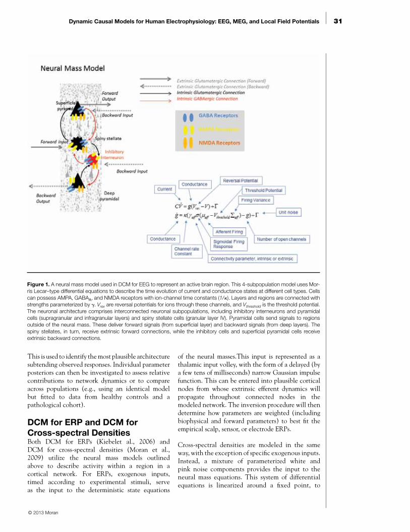
Together, these dynamic descriptions, comprising coupled nonlinear differential equations, form a mathematical state space. These states describe the dynamic elements of a neural mass, such as fluctuations in membrane depolarization. Thus, the states of the neuronal model evolve over time according to the value of a set of neuronal parameters. These parameters include the strength of intrinsic connections within each region, the strength of extrinsic connections, and parameters controlling synaptic adaptation (namely, synaptic time constants) (Fig. 1). A forward-observation model is then required to transform these depolarizations into the observed EEG or MEG output.

Forward Models, Model Comparison, and Hypothesis TestingForward models in these DCMs comprise a linear mixture of depolarizations, which are then transformed via a parameterized lead field into scalp-level or sensor-level data (Fig. 2). This mapping can accommodate different lead fields that depend on the imaging modality (e.g., invasive LFPs or noninvasive EEG and MEG). Since dendrites of interneurons are roughly symmetrically positioned around the cell body, whereas dendrites of pyramidal cells align tangentially to the cortical surface, the net dipolar output is modeled primarily as the output of these pyramidal subpopulations.This fully parameterized generative model can then recapitulate electrophysiological data.

An inversion routine can then be applied to a particular model given empirical EEG/MEG or LFP recordings. The inversion routine is central to the utility of these neural masses and is a fundament of DCM methodology. So far, we have outlined a generative model of electrophysiological data. DCM is designed to map backward from real measured responses to the underlying neuronal generators (Fig. 2). This inverse mapping or model inversion provides an estimation of the model parameters that are conditional on a given set of data. In DCM, this procedure is prescribed by a variational scheme, which optimizes the conditional density of parameters under a fixed-form (Laplace) assumption. This optimization entails using the expectation maximization method to maximize a free-energy bound on the log evidence. The inversion scheme requires both a form for the observation noise (to produce a likelihood function of the modeled parameters) and prior probabilities based on model parameters. These priors are specified in terms of a prior mean and variance (the prior variance determines how far the parameter can move from its prior mean during inversion). Parameters that have been investigated empirically, such as the time constants of different receptors, are ascribed relatively small prior variance. In contrast, flat (higher variance) priors are used for effective connectivity measures to ensure that their posterior estimates are determined primarily by the data.

Once optimized, the inversion routine returns both an approximation to the log-model evidence, known as the “free energy,” and a set of posterior or conditional model parameters. The first of these is used to assess competing hypotheses about the structure of a model, independent of their parameters.

© 2013 Moran

31Dynamic Causal Models for Human Electrophysiology: EEG, MEG, and Local Field Potentials

This is used to identify the most plausible architecture subtending observed responses. Individual parameter posteriors can then be investigated to assess relative contributions to network dynamics or to compare across populations (e.g., using an identical model but fitted to data from healthy controls and a pathological cohort).

DCM for ERP and DCM for Cross-spectral DensitiesBoth DCM for ERPs (Kiebelet al., 2006) and DCM for cross-spectral densities (Moran et al., 2009) utilize the neural mass models outlined above to describe activity within a region in a cortical network. For ERPs, exogenous inputs, timed according to experimental stimuli, serve as the input to the deterministic state equations

of the neural masses.This input is represented as a thalamic input volley, with the form of a delayed (by a few tens of milliseconds) narrow Gaussian impulse function. This can be entered into plausible cortical nodes from whose extrinsic efferent dynamics will propagate throughout connected nodes in the modeled network. The inversion procedure will then determine how parameters are weighted (including biophysical and forward parameters) to best fit the empirical scalp, sensor, or electrode ERPs.

Cross-spectral densities are modeled in the same way, with the exception of specific exogenous inputs. Instead, a mixture of parameterized white and pink noise components provides the input to the neural mass equations. This system of differential equations is linearized around a fixed point, to

© 2013 Moran

Figure 1. A neural mass model used in DCM for EEG to represent an active brain region. This 4-subpopulation model uses Mor-ris Lecar–type differential equations to describe the time evolution of current and conductance states at different cell types. Cells can possess AMPA, GABAA, and NMDA receptors with ion-channel time constants (1/κ). Layers and regions are connected with strengths parameterized by γ. Vrev are reversal potentials for ions through these channels, and Vthreshold is the threshold potential. The neuronal architecture comprises interconnected neuronal subpopulations, including inhibitory interneurons and pyramidal cells (supragranular and infragranular layers) and spiny stellate cells (granular layer IV). Pyramidal cells send signals to regions outside of the neural mass. These deliver forward signals (from superficial layer) and backward signals (from deep layers). The spiny stellates, in turn, receive extrinsic forward connections, while the inhibitory cells and superficial pyramidal cells receive extrinsic backward connections.

32

NoTeS describe the response of a node in the frequency domain. This linearization allows one to compute the transfer function mapping from the endogenous (neuronal) fluctuations to the scalp, sensor, or electrode data. This transformation assumes that the system operates in a stationary regime, with fluctuations around a stable fixed point. The DCM for CSDs also returns coherence, covariance, and phase lags at the level of neuronal sources and the scalp or sensor level.

DCM for Induced Responses and DCM for Phase CouplingDCM for IRs (Chen et al., 2008) and DCM for PHA (Penny et al., 2009) are based on identical principles to those outlined above. These comprise the description of a generative model and the description of priors on model parameters, and Bayesian model inversion. These DCMs are distinct from DCM for ERPs and DCM for CSDs in two ways. The first difference is that they do not explicitly describe a neurobiological architecture in the generative model; instead, they prescribe an abstracted mathematical form that is flexible enough to accommodate highly nonlinear generative mechanisms. The second difference is that data are modeled directly in source

space, so they require preliminary source localization and time-series extraction.

Frequency-to-frequency interactions are a popular topic in human electrophysiological research. For example, it arises when assessing whether alpha spectra suppress other spectral features locally or at different regions of the brain. This type of hypothesis can be addressed formally using a DCM for IR, in which a full time-frequency interaction can be deconstructed using a model of connected brain nodes. DCMs for IR show spectral dynamics in terms of a mixture of frequency modes obtained from source space with singular value decomposition. The differential equations employed in this routine represent the time evolution of energy interactions across all frequencies, where linear or nonlinear source interactions can prescribe within- and between-frequency empirical effects.

To understand how regions of the brain may become phase-locked or drift out of phase, DCM for phase coupling optimizes a generative model comprising weakly coupled oscillators. These sets of differential equations describe how the phase of one region (modeled as an oscillator) influences the change of phase of another. These time-evolving phase

couplings are described in terms of a Fourier series to any order. Given empirical data series from EEG/MEG or LFP, a Hilbert transform of source-space time-series data (band-passed to a frequency of interest) reveals how networks interact in that spectral domain. This is an increasingly studied principle of cortical organization, one prominent example being the investigation of hippocampal-based network interactions in theta and gamma bands.

ConclusionThe DCM approach to analyzing electrophysiological data takes advantage of the large and rich body of literature surrounding neural physiology and neuronal codes. It is an informed analysis method that allows us to formally address how our EEG/MEG/LFP data could have been generated by the brain.

© 2013 Moran

Figure 2. Elements of the DCM framework. Generative models (physiological for DCM for ERP/CSD and phenomenological for DCM for IR/PHA) produce a repertoire of empirical recordings. A particular data set acquired in humans (or animals) can then be fitted to these models using a variational Bayesian inversion, to reveal the density of model parameters conditional on those particular data.

33Dynamic Causal Models for Human Electrophysiology: EEG, MEG, and Local Field Potentials

AcknowledgmentsAll the DCM components described in this chapter can be implemented using MATLAB routines available as part of the academic freeware package SPM (Statistical Parametric Mapping) from http://www.fil.ion.ucl.ac.uk/spm/software/spm12/. This software was written by members and honorary members of the FIL Methods Group at University College London.

ReferencesChen C, Kiebel S, Friston K (2008) Dynamic causal

modelling of induced responses. Neuroimage 41:1293–1312.

Friston K, Harrison L, Penny W (2003) Dynamic causal modelling. Neuroimage 19:1273–1302.

Hodgkin AL, Huxley AF (1952) Propagation of electrical signals along giant nerve fibres. Proc Roy Soc London B Biol Sci 140:177–183.

Kiebel S, David O, Friston K (2006) Dynamic causal modelling of evoked responses in EEG/MEG with lead field parameterization. Neuroimage 30:1273–1284.

Moran RJ, Stephan KE, Seidenbecher T, Pape HC, Dolan RJ, Friston KJ (2009) Dynamic causal models of steady-state responses. Neuroimage 44:796–811.

Penny W, Litvak V, Fuentemilla L, Duzel E, Friston K (2009) Dynamic causal models for phase coupling. J Neurosci Methods 183:19–30.

© 2013 Moran

© 2013

Athinoula A. Martinos Center for Biomedical Imaging Massachusetts General Hospital

Charlestown, Massachusetts

Overcoming Challenges of MEG/EEG Data Analysis: Insights from Biophysics, Anatomy, and Physiology

Matti S. Hämäläinen, PhD

© 2013 Hämäläinen

37Overcoming Challenges of MEG/EEG Data Analysis: Insights from Biophysics, Anatomy, and Physiology

IntroductionBy noninvasively measuring electromagnetic signals ensuing from neurons, magnetoencephalography (MEG) and electroencephalography (EEG) are the only noninvasive human brain imaging tools that provide submillisecond temporal accuracy. In this way, they help to unravel precise dynamics of brain function. Functional magnetic resonance imaging (fMRI) provides a spatial resolution in the millimeter scale, but its temporal resolution is limited because it measures neuronal activity indirectly by imaging the sluggish hemodynamic response. In contrast, MEG and EEG measure the magnetic and electric fields that are directly related to the underlying electrophysiological processes and can thus attain their high temporal resolution.

Processing MEG or EEG data to obtain accurate localization of active neural sources is a complicated task. It involves numerous steps: signal denoising; segmenting various structures from anatomical MRIs; numerical solution of the electromagnetic forward problem; a solution to the ill-posed electromagnetic inverse problem; and appropriate control of multiple statistical comparisons spanning space, time, and frequency across experimental conditions and groups of subjects. This complexity not only constitutes a challenge to MEG investigators but also offers a great deal of flexibility in data analysis.

However, thanks to the direct relationship between the MEG and EEG signals and the underlying neural currents, much insight into these methods can be gained by understanding the associated biophysics in the context of neurophysiology and anatomy. This chapter discusses the relationship of the macroscopic MEG and EEG signals and their physiological sources, thus providing the foundation for understanding the analysis methods applied to estimate the time courses of brain activity. It also gives an overview of available source estimation methods to help beginners understand their underlying assumptions and their applicability to particular experimental data.

Sources and FieldsNeuronal currents generate magnetic and electric fields according to Maxwell’s equations. This current distribution can be described as the primary current, the “battery” if you will, in a resistive circuit that comprises the head. The postsynaptic currents in the cortical pyramidal cells are the main primary currents giving rise to measurable MEG/EEG signals. In many calculations, the head can be approximated with a spherically symmetric conductor; however, more realistic head models for field calculations

can be constructed with the help of anatomical magnetic resonance (MR) or computed tomography (CT) images.

If we employ the spherically symmetric conductor model, the magnetic field of a current dipole can be derived from a simple analytic expression (Sarvas, 1987). An important feature of this sphere model is that the result is independent of the conductivities and thicknesses of the spherical layers; it is sufficient to know the center of symmetry. In contrast, calculating the electric potential is more complicated and requires full information on conductivity. Because radial currents do not produce any magnetic field outside a spherically symmetric conductor, MEG to a great extent is selectively sensitive to tangential sources. EEG data are thus required for recovering all components of the current distribution. Since the resultant current orientation on the cortex is normal to the cortical mantle, MEG is selectively sensitive to fissural activity (Fig. 1).

The analytic sphere model provides accurate enough estimates for many practical purposes. However, when the source areas are located deep within the brain or in frontal areas, it is necessary to use more accurate approaches (Mosher et al., 1999). Within a realistic geometry of the head, the Maxwell’s equations cannot be solved without resorting to numerical techniques. In the boundary-element method (BEM), the electrical conductivity of the head is assumed to be piecewise homogeneous and isotropic. Under these conditions, electric potential and magnetic field can be calculated numerically, starting from integral equations that are discretized to linear matrix equations (Hämäläinen and Sarvas, 1989; Mosher et al., 1999).

The conductivity of the skull is low; therefore, most of the current associated with brain activity is limited to the intracranial space. A highly accurate model for MEG is obtained by considering only one homogeneous compartment bounded by the skull’s inner surface (Hämäläinen and Sarvas, 1989). The boundary-element model for EEG is more complex because at least three compartments need to be considered: the scalp, the skull, and the brain.

It is also possible to employ the finite-element method (FEM) or the finite difference method (FDM) for solving the forward problem. The solution is then based directly on the discretization of the Poisson equation governing the electric potential. In this case, any three-dimensional conductivity distribution and even anisotropic conductivity can be incorporated.

© 2013 Hämäläinen

38

NoTeS

Thanks to improvements to computational methods, FEM approaches are being introduced into routine use in source modeling algorithms that require repeated calculation of the magnetic field from different source distributions (Wolters et al., 2004).

As discussed above, MEG signals can be computed to a high level of accuracy without referring to the particular electrical conductivity values within the head. Therefore, MEG is likely to provide more accurate estimates of the current strengths than EEG. Combined with information about the feasible current densities on the cortex (Okada et al., 1997; Murakami et al., 2002), it is thus possible to infer the sizes of the activated cortical areas. These current density estimates are in the range of 0.1–1.0 nAm/mm2, translating a typical 20 nAm current dipole observed in MEG/EEG to a cortical area of 20–200 mm2.

Sensitivity Characteristics of MEG and EEGIn general, electric and magnetic fields decay as a function of distance from the underlying sources. However, other important factors affect the sensitivity of MEG and EEG to activity in different brain structures. These factors include the organization of the active cell assemblies, effects of the almost spherical symmetry of the head, macroscopic spatial cancellation effects, and extent of temporal coherence of the source activity.

As shown in Figure 1, the cortex has a cellular organization favoring the generation of strong MEG and EEG signals: The pyramidal cells are oriented in parallel and normal to the cortical

mantle, making it possible for the electromagnetic fields from postsynaptic currents in individual cells to add up constructively to produce measurable fields. Such inference is much more difficult to make for small deeper structures, even though it has been clearly shown that both EEG and MEG signals can be produced, for example, by the brainstem nuclei (Parkkonen et al., 2009). Using simulations, it also has been shown that, in the absence of simultaneous cortical activity, hippocampal activity can

be detected with standard source localization methods (Attal and Schwartz, 2013). The same study also found that it is possible to detect weak thalamic modulations of ongoing activity. Furthermore, MEG has provided insights into the specific dissociated neural pathways involved in emotion and face perception, including sources in both the cortex and the amygdalae (Hung et al., 2010).

It is important to note that since the spherically symmetrical conductor model well approximates the computation of MEG/EEG, the overall conclusion regarding the relative sensitivities of the two methods remains valid even in a more realistic head model. Figure 2 illustrates the distribution of MEG and EEG sensitivity across the cortex when the signals are

© 2013 Hämäläinen

Primary currents

MEG = 0

MEG ≠ 0EEG ≠ 0

EEG ≠ 0

cortex

current sources

Figure 1. Principal orientation of primary currents on the cortex (left). Differential sen-sitivity of MEG and EEG in the presence of cortical folding (right).

Figure 2. The power of the MEG (left) and EEG (right) signal patterns mea-sured with 102 magnetometers (left) and 60 EEG electrodes (right) generated by current sources normal to the cortex. The maximal value of each distribu-tion is normalized to unity, i.e., the scale bars show fractions of the maximum value. Notice the strong contribution that sources at the crests of the gyri make to EEG and the steep falloff of the MEG signal with depth.

39

computed using a three-compartment BEM rather than the sphere model. MEG indeed appears almost blind to sources at the crests of the gyri and those at the bottom of the sulci, whereas EEG receives a very strong contribution from the radially oriented gyral sources. This discrepancy means that the signal-to-noise ratio (SNR) of EEG for activity in the sulci is likely to be lower than that of MEG. In a study by Goldenholz et al. (2009), theoretical calculations were further supported by evidence from observations of variable SNRs of epileptic spikes as a function of their location of origin. Figure 2 also clearly shows that deep sources are more weakly reflected in MEG than in EEG. However, as discussed in Attal and Schwartz (2013) and supported by the evidence of MEG being able to detect signals from the deeper structures discussed earlier, the SNR of MEG and that of EEG may be more similar than generally thought.

Because the cortex is heavily folded, MEG and EEG signals originating from the synchronous activation of a large region of cortex probably suffer from cancellation effects due to different source orientations being present. These spatial cancellation effects were recently studied in detail (Ahlfors et al., 2010). The results indicate that both MEG and EEG signals are strongly attenuated because of cortical folding. Also, this attenuation is more significant in MEG than in EEG, when a large ensemble of patches at different locations of the cortex is considered. The reason for the latter difference is most likely the contribution that radial sources make to EEG. In particular, if the activated patch includes a crest of a gyrus and walls of fissures symmetrically on both sides of it, the MEG signals arising from the fissural cortex are canceled out, while the EEG signals arising from the radially oriented currents remain. This phenomenon is illustrated in Figure 3, which simulates the signals arising from the activation of a large patch in the parietal cortex, covering both walls of fissures. The EEG signals indicate the presence of radial currents at the activated site, whereas MEG detects only minor tangential sources in the “outskirts” of the activated patch.

The Equivalent-Current Dipole ModelsThe goal of the electromagnetic inverse problem is to estimate the source-current density underlying the MEG or EEG signals measured outside the head. Unfortunately, the primary current distribution cannot be recovered uniquely, even if the magnetic field and/or the electric potential were precisely known everywhere outside the head (Helmholtz, 1853). However, it is often possible to use additional

anatomical and physiological information to constrain the problem and to facilitate its solution. One approach is to replace the actual current sources by equivalent generators that are characterized by a few parameters. A unique solution for the parameters may then be obtained from the measured data by a least squares fit. Figure 4 illustrates the concept of the equivalent-current dipole (ECD) source. In this simulation, an extended patch of cortex near the left auditory cortex was activated, and the ECD was fitted to the simulated data. The location of the dipole matches the site of activation well, even though the information of the actual extent is naturally lost.

In the time-varying dipole model, first introduced to the analysis of EEG data (Scherg and von Cramon, 1985; Scherg, 1990), an epoch of data is modeled with a set of current dipoles whose orientations and locations are fixed but whose amplitudes are allowed to vary with time. This approach corresponds to the idea of small patches of the cerebral cortex or other structures being activated simultaneously or in a sequence. As noted, the precise details of the current distribution within each patch cannot be revealed by the measurements, which are performed at a distance in excess of 3 cm from the sources.

Overcoming Challenges of MEG/EEG Data Analysis: Insights from Biophysics, Anatomy, and Physiology

© 2013 Hämäläinen

MEG

(a) (b)

(d)(c)

EEG

Figure 3. MEG (a) and EEG (b) signal distributions arising from the activation of a patch of parietal cortex. In a, the red and blue contours indicate magnetic emerging and entering the head, respectively, while in b, red and blue indicate the positive and negative potential values. The corresponding minimum-norm current estimates were computed with a cortical constraint and are visualized in an inflated view of the cortex in c and d. The activated area is shown with green shading. EEG shows activity in cortex with radially oriented currents (light gray areas), whereas the MEG-visible currents in the fissures are largely invisible owing to cancellation between the opposite walls of the sulci.

40

NoTeS

Distributed Source ModelsAn alternative approach to source modeling is to assume that the sources are distributed within a volume or surface (often called the source space) and then to use various estimation techniques to find out the most plausible source distribution. The source space may be either a volume defined by the brain or restricted to the cerebral cortex, determined from MR images (Dale et al., 1999). These techniques can provide reasonable estimates of complex source configurations without having to resort to complicated dipole-fitting strategies.

Inverse solutions that result in a source distribution are commonly referred to as “imaging methods.” This nomenclature is motivated by the fact that the current estimate explains the data and can be visualized as an image or a sequence of images. If the sources are limited to the cortex, their orientations can be aligned with the estimated cortical surface normals (Dale and Sereno, 1993). In this case, only the dipole amplitudes need to be estimated. Alternatively, the orientations can be considered unknown, in which case both amplitudes and orientations need to be estimated at each spatial location.

One of the challenges for distributed inverse methods is that the number of dipoles by far exceeds the number of MEG/EEG sensors. Therefore, a priori constraints based on the likely characteristics of the actual source distributions are necessary. Common priors are based on the Frobenius norm and lead to a family of methods generally referred to as minimum-norm estimates (MNEs) (Hämäläinen and Ilmoniemi, 1984). MNEs can be converted into statistical parameter maps, which take into account the noise level, leading to noise-normalized methods such as dSPM (dynamic statistical parametric mapping) (Dale et al., 2000)

or sLORETA (standardized low-resolution electromagnetic tomography) (Pascual-Marqui, 2002).

Although these methods have clear benefits, including simple implementation and robustness to noise, they do not take into account the natural assumption that only a few brain regions are typically active during a task. Interestingly, this latter assumption is exactly what justifies the use of discrete dipole-fitting methods. In order to promote such focal or sparse solutions within the distributed source model framework, one uses sparsity-inducing priors (Matsuura

and Okabe, 1995; Uutela et al., 1999). However, if such priors are applied time point by time point (using minimum-current estimates, or MCEs), it becomes challenging to obtain consistent estimates of the source orientations as well as temporally meaningful source waveforms.

In order to promote spatiotemporally coherent focal estimates, several publications have proposed constraining the active sources to remain the same over the time interval of interest (Friston et al., 2008; Ou et al., 2009; Wipf and Nagarajan, 2009; Gramfort et al., 2012). The implicit assumption then becomes that the sources are stationary. This conjecture is reasonable for short time intervals. However, it is not a good model for realistic source configurations where multiple transient sources activate sequentially or simultaneously during the analysis period before returning to baseline at different time instants.

We recently addressed the problem of localizing nonstationary focal sources from MEG/EEG data using appropriate sparsity-inducing norms (Gramfort et al., 2013). Extending the work from Gramfort et al. (2012) in which we coined the term “mixed-norm estimates” (MxNEs), we proposed in Gramfort et al. (2013) to use mixed norms defined in terms of the time-frequency decompositions of the sources. We called this approach the time-frequency mixed-norms estimates (TF-MxNE). The benefit of this modification is that the estimates of nonstationary sources can be obtained over longer time intervals while making optional standard preprocessing (e.g., filtering or time-frequency analysis of the sensor signals).

Figure 5 summarizes the spatiotemporal character-istics of different distributed source estimates. The

© 2013 Hämäläinen

Figure 4. An equivalent-current dipole (green dot) corresponding to an activated patch of cortex (red shading). A, anterior; R, right; S, superior.

s

R A

41

MNE solutions and statistical maps derived there-from exhibit nonzero activity at all time points and spatial locations. Therefore, the extents of the ac-tivity depend on the statistical thresholding applied. The MCE solution is a sparse estimate computed separately at each time point and, therefore, spatial consistency across time is not warranted. The MxNE solution posited by Ou et al. (2009) and Gramfort et al. (2012) shows consistent locations of activity, but the source amplitudes are nonzero at all time points. Finally, the TF-MxNE solution is sparse in space and locally smooth in time/frequency but allows for non-stationarity of the sources on the global time scale.

ConclusionsSince the relationship of MEG or EEG signals and their sources is fully governed by the Maxwell’s equations, the signal distributions arising from given cerebral sources can be simulated accurately. These simulations give several insights into the characteristics of MEG and EEG. For example, MEG is less sensitive to the actual electrical conductivities within the head, and EEG and can thus provide more accurate estimates of the source strengths than can MEG. Furthermore, although MEG receives weaker contributions from deep sources within the brain than EEG, the SNRs of MEG and EEG may actually be similar. The similarity derives from the strong EEG signals arising from very superficial cortical activity; these signals, in turn, are filtered out from MEG owing to the radial orientation of the corresponding sources.

The ambiguity of the inverse problem has been often cited as a major drawback of both EEG and MEG. Both methods thus have had to rely on a restrictive source model, making the analysis rather difficult for a beginner. It is also perhaps confusing to find that several competing source models are available, and sometimes, the authors introducing them are not clear enough about stating the underlying assumptions and their consequences for data interpretation. Fortunately, constraints for the inverse problem can be obtained from other imaging modalities, in particular, anatomical MRI.

We expect in the future major developments in efficient and automated MEG/EEG analysis methods, novel experimental paradigms to fully utilize the benefits of MEG/EEG, and reliable routines to combine MEG/EEG with other imaging modalities. We anticipate that such approaches will significantly increase our understanding of human brain functions, especially their temporal dynamics and the interactions between cortical regions and deeper structures involved in perception, cognition, and action.

ReferencesAhlfors SP, Han J, Lin FH, Witzel T, Belliveau JW,

Hamalainen MS, Halgren E (2010) Cancellation of EEG and MEG signals generated by extended and distributed sources. Hum Brain Mapp 31:140–149.

Attal Y, Schwartz D (2013) Assessment of subcortical source localization using deep brain activity imaging model with minimum norm operators: a MEG study. PloS One 8:e59856.

Dale AM, Sereno MI (1993) Improved localization of cortical activity by combining EEG and MEG with MRI cortical surface reconstruction: a linear approach. J Cogn Neurosci 5:162–176.

Dale AM, Fischl B, Sereno MI (1999) Cortical surface-based analysis. I. Segmentation and surface reconstruction. Neuroimage 9:179–194.

Dale AM, Liu AK, Fischl BR, Buckner RL, Belliveau JW, Lewine JD, Halgren E (2000) Dynamic statistical parametric mapping: combining fMRI and MEG for high-resolution imaging of cortical activity. Neuron 26:55–67.

Friston K, Harrison L, Daunizeau J, Kiebel S, Phillips C, Trujillo-Barreto N, Henson R, Flandin G, Mattout J (2008) Multiple sparse priors for the M/EEG inverse problem. Neuroimage 39:1104–1120.

Overcoming Challenges of MEG/EEG Data Analysis: Insights from Biophysics, Anatomy, and Physiology

© 2013 Hämäläinen

Figure 5. Characteristics of distributed source estimates. MNE, minimum-norm estimate; MCE, minimum current esti-mate; MxNE, mixed-norm estimate promoting spatial sparsity and temporal smoothness; TF-MxNE, time-frequency mixed-norm estimate allowing for nonstationary time courses.

42

NoTeS Goldenholz DM, Ahlfors SP, Hamalainen MS, Sharon D, Ishitobi M, Vaina LM, Stufflebeam SM (2009) Mapping the signal-to-noise-ratios of cortical sources in magnetoencephalography and electroencephalography. Hum Brain Mapp 30:1077–1086.

Gramfort A, Kowalski M, Hamalainen M (2012) Mixed-norm estimates for the M/EEG inverse problem using accelerated gradient methods. Phys Med Biol 57:1937–1961.

Gramfort A, Strohmeier D, Haueisen J, Hamalainen MS, Kowalski M (2013) Time-frequency mixed-norm estimates: sparse M/EEG imaging with non-stationary source activations. Neuroimage 70:410–422.

Hämäläinen M, Ilmoniemi R (1984) Interpreting magnetic fields of the brain: minimum norm estimates. Med Biol Eng Comput 32(1):35–42.

Hämäläinen MS, Sarvas J (1989) Realistic conductivity geometry model of the human head for interpretation of neuromagnetic data. IEEE Trans Biomed Eng 36(2):165–171.

Helmholtz H (1853) Ueber einige Gesetze der Vertheilung elektrischer Strome in korperlichen Leitern, mit Anwendung auf die thierisch-elektrischen Versuche. Ann Phys Chem 89:211–233, 353–377.

Hung Y, Smith ML, Bayle DJ, Mills T, Cheyne D, Taylor MJ (2010) Unattended emotional faces elicit early lateralized amygdala-frontal and fusiform activations. Neuroimage 50:727–733.

Matsuura K, Okabe Y (1995) Selective minimum-norm solution of the biomagnetic inverse problem. IEEE Trans Biomed Eng 42:608–615.

Mosher JC, Leahy RM, Lewis PS (1999) EEG and MEG: forward solutions for inverse methods. IEEE Trans Biomed Eng 46:245–259.

Murakami S, Zhang T, Hirose A, Okada YC (2002) Physiological origins of evoked magnetic fields and extracellular field potentials produced by guinea-pig CA3 hippocampal slices. J Physiol 544:237–251.

Okada YC, Wu J, Kyuhou S (1997) Genesis of MEG signals in a mammalian CNS structure. Electroencephalogr Clin Neurophysiol 103:474–485.

Ou W, Hamalainen MS, Golland P (2009) A distributed spatio-temporal EEG/MEG inverse solver. Neuroimage 44:932–946.

Parkkonen L, Fujiki N, Makela JP (2009) Sources

of auditory brainstem responses revisited: contribution by magnetoencephalography. Hum Brain Mapp 30:1772–1782.

Pascual-Marqui RD (2002) Standardized low-resolution brain electromagnetic tomography (sLORETA): technical details. Methods Find Exp Clin Pharmacol 24(Suppl D):5–12.

Sarvas J (1987) Basic mathematical and electromagnetic concepts of the biomagnetic inverse problem. Phys Med Biol 32:11–22.

Scherg M (1990) Fundamentals of dipole source potential analysis. In: Auditory evoked magnetic fields and potentials (Grandori F, Hoke M, Romani GL, eds), pp 40–69. Basel: Karger.

Scherg M, von Cramon D (1985) Two bilateral sources of the late AEP as identified by a spatio-temporal dipole model. Electroencephalogr Clin Neurophysiol 62:232–244.

Uutela K, Hämäläinen M, Somersalo E (1999) Visualization of magnetoencephalographic data using minimum current estimates. Neuroimage 10:173–180.

Wipf D, Nagarajan S (2009) A unified Bayesian framework for MEG/EEG source imaging. Neuroimage 44:947–966.

Wolters CH, Grasedyck L, Hackbusch W (2004) Efficient computation of lead field bases and influence matrix for the FEM-based EEG and MEG inverse problem. Inverse Problems 20:1099–1116.

© 2013 Hämäläinen

© 2013

Department of Psychology University of Texas at Austin

Austin, Texas

Considerations When Using Single-Trial Parameter Estimates in

Representational Similarity AnalysesJeanette A. Mumford, PhD

© 2013 Mumford

45

© 2013 Mumford

Considerations When Using Single-Trial Parameter Estimates in Representational Similarity Analyses

IntroductionTraditional analyses of functional magnetic resonance imaging (fMRI) data compare mean blood-oxygen-level–dependent (BOLD) activations during different tasks to determine where brain activation differences occur. More recently, the patterns of activation within regions of the brain have been studied with keen interest. In them, the input patterns consist of either the test statistics or the activation estimate magnitudes associated with a task over space (Haxby, 2001; Carlson et al., 2003; Pereira et al., 2009; Kriegeskorte et al., 2008; Kriegeskorte, 2011). The two most common pattern analyses are multivariate pattern classification analyses and pattern similarity analyses, which are commonly referred to as representational similarity analyses (RSAs).

Multivariate pattern classification analyses use activation patterns, either over the entire brain or within a region of interest (ROI). They use a cross-validation approach, where part of the data is used to train a model that discerns between different task patterns; then, this fitted model is used to predict the task associated with another set of independent patterns, ignoring their labels. The performance of the model is assessed by the accuracy of the predictions. The models used include regularized logistic regression and support vector machine-based classification algorithms (Carlson et al., 2003; Pereira et al., 2009). RSAs correlate activation patterns over space with different tasks to assess the similarity in activation patterns. One can then compare the RSA values, which consist of all possible pairwise correlations between tasks, across different regions of interest and between different imaging modalities (Kriegeskorte et al., 2008; Kriegeskorte, 2011). For example, in Kriegeskorte et al. (2008), RSA-based networks were used to compare human and primate network similarities. The activation patterns used in classification and similarity analyses can be based on estimates for individual trials, as well as windows of time surrounding a trial, and be

aggregated over many trials (Xue et al., 2010; Mumford et al., 2012; Turner et al., 2012).

Because RSA analyses are a newer type in the field, the methods for data analysis have not yet been perfected. The focus here is on RSA analyses that use single-trial activation patterns to generate similarity matrices. For example, a single run of the paradigm might include presenting images of 30 faces and 30 houses, and the goal is then to compute a 60 × 60 similarity matrix to be used in the analysis. This type of approach has been used in the past for designs in which the trials are temporally spaced (Kriegeskorte et al., 2008; Jenkins and Ranganath, 2010; Xue et al., 2010; Ritchey et al., 2012). Recent work has developed methods for obtaining single-trial parameter estimates for faster event–related designs that have improved performance in classification based analyses (Mumford et al., 2012). Therefore, it is only natural that these models be used in RSA-based analyses. This chapter discusses the methods for obtaining single-trial parameter estimates as well as possible problems that can arise when these estimates are used in RSA analyses.

Modeling Single-Trial Activation PatternsObtaining single-trial parameter estimates can be difficult in studies where the stimuli are presented with a short interstimulus interval (ISI). This is because the blurring and delayed nature of the BOLD fMRI signal makes it difficult to isolate a signal that is unique to a specific trial. Previous work introduced a new approach for estimating single-trial parameter estimates in fast event–related designs: using a separate model for each trial and iteratively estimating the pattern for each trial separately. This method is referred to as least squares single (LSS) and is illustrated in the right panel of Figure 1 (Mumford et al., 2012). This method was shown to produce less

Figure 1. Model illustration for LSA and LSS. In both cases, trial-specific activations are estimated for each of 10 trials, and the model is run in a voxelwise fashion. The left panel shows LSA, which estimates all trials simultaneously in a single regression, and the estimates β1, …, β10, which represent the activation magnitudes for each trial. The right panel shows LSS, where each trial's activation is estimated in a separate model. The first regressor represents the trial of interest, and the two additional regressors model the remaining trials according to trial type (in this case, two). Only the estimates for the first parameter are retained from each model.

XLSA β XLSA β

β1

β2

::β10

β1

βTrial1βTrial2

Trial 1

. . .

β10βTrial1βTrial2

Trial N

XLSS1 β XLSS10 β . . .

Least Squares All (LSA)

Least Squares Single (LSS)

XLSA β XLSA β

β1

β2

::β10

β1

βTrial1βTrial2

Trial 1

. . .

β10βTrial1βTrial2

Trial N

XLSS1 β XLSS10 β . . .

Least Squares All (LSA)

Least Squares Single (LSS)

46

NoTeS variable estimates than the more standard approach, which estimates all trials simultaneously in a single model. The standard approach is referred to as least squares all (LSA) and is illustrated in the left panel of Figure 1. Although the behavior and performance of LSS and LSA estimates were studied within the context of pattern classification analyses, they have not been studied within the RSA setting.

Factors That Influence RSA MeasuresNoise differencesSince the RSA measure is based on correlations between activation patterns, it is susceptible to noise differences. For example, if similarity matrices are obtained for multiple ROIs, and one is interested in studying the correlation of the RSA matrices between ROIs (Kriegeskorte et al., 2008; Diedrichsen et al., 2011), then noise variations between regions can induce false-positive differences. For example, if one region has noisier data than another, but the theoretical correlations of the within-region RSA are identical for the two regions, then the noisier region will have smaller RSA values than the other. This problem was discussed by Kriegeskorte et al. (2008), who concluded that a rank-based correlation is necessary to avoid correlation magnitude differences when comparing RSAs between regions. It was also addressed by Diedrichsen et al. (2011), who used a random-effects model to estimate the RSA correlations within regions, adjusting for noise differences. Theoretically, this method would allow for directly comparing RSA values between regions, because it would remove any biases induced by noise differences.

Variability differencesAlthough spatial noise differences and their impact on RSA estimates have been studied, variability differences across trial pattern estimates also can induce false-positive RSA differences within a region of interest. For example, assume that a study has 30 presentations of each of two trials (type 1 and type 2). The T1 trials have a longer duration than the T2 trials, and the RSA study of interest is how the distributions of within-trial RSA values compare between these two trials. It is well known that longer trials yield more efficient estimates of BOLD activation when using the general linear model (GLM), so trial A will have less variable activation-pattern estimates than trial B (Smith et al., 2007). Even if the true within-trial correlation were identical for both trial types, the higher variability in T2’s estimates would lead to within-trial RSA values lower for T2 than for T1. This is not the only case where variability differences may occur between trials, within a region of interest. If the ISI (duration of the baseline task surrounding each trial) differs between trials, shorter trials will also have noisier activation-pattern estimates.

Model influence A less studied phenomenon is how the model itself can determine correlations between activation patterns. This is the case for both LSS and LSA methods for obtaining activation patterns for single trials. Figure 2 illustrates the true RSA values between 60 trials (the first 30 trials are type 1 and second set of 30 are type 2), where a correlation of 0 is assumed between all trials, and the ISI is equal for all trials and 2 s on average (left panel). The middle and right panels show the theoretical correlations

© 2013 Mumford

Figure 2. RSA estimate comparisons for the null case. The run consisted of 20 trials, each 2 s long with a random ISI between 2 s and 4 s. There were two trial types: 30 of trial type 1, followed by 30 of trial type B. Trials are ordered in the matrices as they were presented in time, starting from trial 1 (bottom left corner) to trial 60 (top right corner). Each cell in the matrix corresponds to the correlation between activation patterns between two trials. The left panel illustrates the true RSA, which in this case of the null is set to an identity matrix (1s on diagonal and 0s elsewhere). The middle and left panels are the LSA- and LSS-based RSA matrices that were theoretically derived.

10 20 30 40 50 60

1020

3040

5060

Truth

Trial Number

Tria

l Num

ber

10 20 30 40 50 60

1020

3040

5060

LSA

Trial Number

Tria

l Num

ber

10 20 30 40 50 60

1020

3040

5060

LSS

Trial Number

Tria

l Num

ber

−0.4

−0.2

0.0

0.2

0.4

0.6

0.8

1.0

47

between the activation patterns when using LSA and LSS, respectively. In these graphs, the trials are ordered temporally from first to last, from the bottom left corner to the top right corner of the plot. The first off-diagonal of the plot, therefore, indicates the lag 1 correlations between trials.

As this figure shows, for both LSS and LSA, there is a bias in the lag 1 correlation. In LSS, trials that are temporally adjacent (lag 1) are anticorrelated, since the collinearity in the model pushes the estimate of one trial in the opposite direction of its collinear neighbors. In contrast, LSA has a positive bias that occurs because the trials are modeled separately and, hence, are not adjusted for each other statistically and thus describe similar parts of the data. LSS shows a blocked pattern caused by a collinearity effect in the LSS model that occurs when the neighbors of a trial match each other, but not necessarily the trial in the middle. This causes a weak negative correlation between that trial and all trials of the neighbors’ type, owing to a collinearity between the single trial and the nuisance regressor for the trial of the neighbors’ type. The fact that trials are blocked in Figure 2 causes a weak negative correlation between all trials of the same type, though correlations between trial types are comparatively more positive—a counterintuitive result. These patterns are described in more detail for a variety of trial orderings and ISI durations below.

Trial order and ISI durationA series of simulations were used to study how the patterns in Figure 2 vary as a function of the ordering of the trials and the ISI duration. Trials were either blocked (all trial 1, followed by all trial 2), alternated (T1, T2, T1, etc.), or randomly generated for each

run. Situations where the ISIs matched between trials and when the ISI was longer for T2 were investigated. The ISIs were randomly drawn from continuous uniform distributions, where U(a,b) represented random draws between a and b. The TR used in the simulations was 2 s.

To start, the behavior of the correlation as a function of lag was estimated. Figure 3 shows the mean correlation as a function of lag for ISIs ranging between 2 s and 7 s, where ISIs matched for the two trial types. The left panel shows the patterns for LSA, in which for an ISI of 2 (red line), the correlation alternates between negative and positive. This pattern results from collinearity pushing neighboring trials in opposite directions. Thus, at a lag of 1, the correlation would be negative, but at a lag of 2, there is a positive correlation (since both trials would be pushed in the same direction by their common collinear neighbor). This effect diminishes as the ISI increases, since the collinearity problem is reduced. Even so, the mean correlation is never the true correlation of 0 but hovers around 0.1—the result of the influence of the model itself.

The LSS model shows positive correlations for early lags owing to the overlap in the trials, which are not statistically adjusted for each other and hence describe the same variability in the data. The dip around a lag of 3 when the ISI equals 2 results from the peak of one trial meeting the poststimulus undershoot of another, a difference of approximately 6 s.

The results in Figure 4 compare within-trial correlations (red and green) to between-trial correlations (blue) when the ISIs match and when T2’s ISIs are longer

Considerations When Using Single-Trial Parameter Estimates in Representational Similarity Analyses

© 2013 Mumford

Figure 3. Averaged correlations as a function of lag for LSA (left) and LSS (right) for varying ISIs when trials are blocked. LSA tends to alternate between positive and negative due to collinearity; in contrast, LSS tends to have high positive correlations at early lags, followed by a negative correlation when the peak of one trial meets with the poststimulus undershoot of another trial.

2 4 6 8 10 2 4 6 8 10

−0.3

−0.2

−0.1

0.0

0.1

0.2

LSA

Lag

Mea

n co

rrela

tion

mean ISI=2mean ISI=3mean ISI=4mean ISI=5mean ISI=6mean ISI=7

0.0

0.1

0.2

0.3

0.4

0.5

LSS

Lag

Mea

n co

rrela

tion

48

NoTeS

for blocked (left), alternating (middle), and random (right) trial orderings. Significantly, in the random setting (right), each run had a different randomization. The top row shows the LSA results, and the bottom shows LSS ones. The alternating blocked designs illustrate that, even with the ISIs matching, the within-trial correlations are not comparable with the between-trial correlations. In the alternating LSA, the within-trial correlations are larger; in the blocked case, they are smaller, as noted in Figure 1. When the ISIs differ between trials, there is not much impact in the alternating case since, on average, each trial has the same amount of fixation or rest on either side of it. In both the blocked and random cases, the second trial type will always have more fixation surrounding it, which decreases the collinearity problem for trials of type 2, removing some bias in the correlation estimate. The only case where the correlations are comparable for both LSA and LSS is when the ISIs match and the trial order is randomized.

Randomly ordering trials and matching the ISI seem to be key for both LSS and LSA; however, it is important that the trials be randomly ordered for each run of the analysis. In reality, it is common to generate one or two trial orderings found to be efficient for the design and to use these for all subjects. But when this is done, slight biases in ISI may occur.

In 100 simulated data sets with 40 subjects in each study, more than half of the data sets exhibited a statistically significant difference between at least one of the pairwise comparisons (within T1 versus within T2; within T1 versus between T1/T2; or within T2 versus between T1/T2). Figure 5 illustrates the distribution of RSA values for a single one of these simulated data sets. It shows that the within-T2 correlations are significantly larger than both within-T1 and between-T1/T2 ones. Although the magnitude of the difference is quite small, it is common to look only at the p values of these tests, so this would not be taken into consideration.

Possible Remedies and ConsiderationsOne possible fix for this problem is to compute RSA matrices by using comparisons of patterns estimated with different models. For example, if there are two runs of a study for a single subject, correlate only a single trial’s pattern from run 1 with trials in run 2. Since the biases discussed above were all imposed by the models used, this will prevent that bias from entering the analysis. Notably, however, this will not solve problems where the ISI was not equal across all trial types.

© 2013 Mumford

Figure 4. Distributions of within-trial and between-trial correlations for 100 simulated data sets for varying ISI settings and trial orderings for LSA (top) and LSS (bottom). The setting of equal ISIs with random trial orderings appears to remove biases, as-suming that a different randomization is used for each subject.

LSA:Blocked LSA:Alternating LSA:Random

LSS:Blocked LSS:Alternating LSS:Random

0.050

0.075

0.100

0.125

0.050

0.075

0.100

0.125

U(2,4)/U(2,4) U(2,4)/U(4,6) U(2,4)/U(2,4) U(2,4)/U(4,6) U(2,4)/U(2,4) U(2,4)/U(4,6)ISI

Cor

rela

tion

Correlation Typewithin T1within T2btwn T1/T2

49

Before running a study, it is fairly easy to take the proposed paradigm and perform simulations like the ones run here to investigate possible biases that may enter the analysis. However, using between-run correlations should remedy many of the problems. What is important is to recognize that paradigms that work very well when studying activation magnitudes and their differences may not work as well in the RSA setting. Although only ISI differences were studied here, the same problems would arise if there were differences in the duration of the stimuli. Where stimulus presentation is controlled by the reaction time of the subject, further analysis strategies would need to be developed to control for those differences.

ReferencesCarlson TA, Schrater P, He S (2003) Patterns of

activity in the categorical representations of objects. J Cogn Neurosci 15:704–717.

Diedrichsen J, Ridgway GR, Friston KJ, Wiestler T (2011) Comparing the similarity and spatial structure of neural representations: a pattern-component model. Neuroimage 55:1665–1678.

Haxby JV (2001) Distributed and overlapping representations of faces and objects in ventral temporal cortex. Science 293:2425–2430.

Jenkins LJ, Ranganath C (2010) Prefrontal and medial temporal lobe activity at encoding predicts temporal context memory. J Neurosci 30:15558–15565.

Kriegeskorte N (2011) Pattern-information analysis: From stimulus decoding to computational-model testing. Neuroimage 56:411–421. Available at http://linkinghub.elsevier.com/retrieve/pii/S10538 11911000978.

Kriegeskorte N, Mur M, Bandettini P (2008) Representational similarity analysis—connecting the branches of systems neuroscience. Front Sys Neurosci 2:4.

Mumford JA, Turner BO, Ashby FG, Poldrack RA (2012) Deconvolving BOLD activation in event-related designs for multivoxel pattern classification analyses. Neuroimage 59:2636–2643.

Pereira F, Mitchell T, Botvinick M (2009) Machine learning classifiers and fMRI: a tutorial overview. Neuroimage 45:S199–S209.

Ritchey M, Wing EA, LaBar KS, Cabeza R (2012) Neural similarity between encoding and retrieval is related to memory via hippocampal interactions. cerebral cortex. 2012 Sep 11. [Epub ahead of print]

Considerations When Using Single-Trial Parameter Estimates in Representational Similarity Analyses

© 2013 Mumford

Figure 5. When the same randomization is used across all subjects, unusual patterns can emerge that cause small yet statisti-cally significant differences in RSA distributions. In this case, the within-T2 similarities appear larger than within-T1 and between-T1/T2 similarities, when theoretically, they all equal 0.

LSA LSS

0.085

0.090

0.095

0.100

0.105

0.110

0.115

U(2,4)/U(2,4) U(2,4)/U(2,4)ISI

Cor

rela

tion

Correlation Typewithin T1within T2btwn T1/T2

© 2013

50

NoTeS Smith S, Jenkinson M, Beckmann C, Miller K, Woolrich M (2007) Meaningful design and contrast estimability in FMRI. Neuroimage 34:127–136.

Turner BO, Mumford JA, Poldrack RA, Ashby FG (2012) Spatiotemporal activity estimation for multivoxel pattern analysis with rapid event-related designs. Neuroimage 62:1429–1438.

Xue G, Dong Q, Chen C, Lu Z, Mumford JA, Poldrack RA (2010) Greater neural pattern similarity across repetitions is associated with better memory. Science 330:97–101.