neurominer manual - pronia€¦ · neurominer manual pronia, personalized prognostic tools for...
TRANSCRIPT

NeuroMiner Manual
PRONIA, Personalized Prognostic Tools forEarly Psychosis Management
Ludwig-Maximilians-Universtitat, MunchenSoftware written by Nikolaos Koutsouleris
Manual written by Dom DwyerFormatting, testing, and additional writing:Carlos Cabral, Shalaila Haas, Anne Ruef
Additional testing:Maria Urquijo, Joseph Kambeitz,
Lana Kambeitz-Ilankovic,Ana Tupac, Johanna Weiske,
Jing Shang, Janos Kalman,& the PRONIA consortium.
Date: 27th April 2017Version 1.1
Contents
1 Introduction 1
2 Suggested Prerequisites 4
3 Getting Started 6
3.1 Compatibility . . . . . . . . . . . . . . . . . . . . . . . . . . . 6
3.2 Downloading and Initialising NeuroMiner . . . . . . . . . . . . 6
3.3 Nomenclature . . . . . . . . . . . . . . . . . . . . . . . . . . 6
4 Main Interface 8
4.1 Input data into NM . . . . . . . . . . . . . . . . . . . . . . . . 12
4.2 Define parameter template . . . . . . . . . . . . . . . . . . . 22
4.3 Multi-group analyses . . . . . . . . . . . . . . . . . . . . . . . 52
4.4 Stacking . . . . . . . . . . . . . . . . . . . . . . . . . . . . . 53
4.5 Initialize analyses . . . . . . . . . . . . . . . . . . . . . . . . 54
4.6 Preprocess features . . . . . . . . . . . . . . . . . . . . . . . 57
4.7 Train supervised classifiers . . . . . . . . . . . . . . . . . . . 58
4.8 Visualize classifiers . . . . . . . . . . . . . . . . . . . . . . . 59
4.9 Display training results . . . . . . . . . . . . . . . . . . . . . . 60
i

4.10 Generate master files . . . . . . . . . . . . . . . . . . . . . . 66
4.11 Out of Sample Cross-Validation . . . . . . . . . . . . . . . . . 66
4.12 Load NeuroMiner structure . . . . . . . . . . . . . . . . . . . 67
4.13 Save NeuroMiner structure . . . . . . . . . . . . . . . . . . . 67
4.14 Clear NeuroMiner structure . . . . . . . . . . . . . . . . . . . 67
4.15 Change Working Directory . . . . . . . . . . . . . . . . . . . . 67
4.16 Open Manual . . . . . . . . . . . . . . . . . . . . . . . . . . . 67
4.17 Utilities . . . . . . . . . . . . . . . . . . . . . . . . . . . . . . 67
5 Example 69
6 Known Issues 77
ii NeuroMiner Manual

1 Introduction
Machine learning techniques are poised to become clinically useful methods
that may be used for diagnosis, prognosis, and treatment decisions. Despite
this, they are currently underutilised in medical studies and, even more in psy-
chiatric research because most current tools require strong programming and
computational engineering skills (e.g., scikit-learn, caret, Weka, nilearn). While
there are some great tools that do not require programming experience (e.g.,
PRoNTo), these are often focused on making predictions from specific data
domains such as neuroimaging data. This highlights a pressing need for user-
friendly machine learning software that makes advanced methods available to
clinical researchers from different fields aiming at collaboratively developing
diagnostic, predictive, and prognostic tools for precision medicine approaches.
NeuroMiner has been continuously developed by Nikolaos Koutsouleris since
2009 (with support from the European Commission for the PRONIA project
since 2013) to provide clinical researchers with cutting-edge machine learning
methods for the analysis of heterogeneous data domains, such as clinical and
neurocognitive read-outs, structural and functional neuroimaging data, and ge-
netic information. The program can be considered as an interface to a large va-
riety of unsupervised, and supervised pattern recognition algorithms that have
been developed in the machine learning field over the last decades. Further-
more, the application implements itself different strategies for preprocessing,
filtering and fusing heterogeneous data, training ensembles of predictors and
visualizing and testing the significance of the computed predictive patterns.
The current release candidate of NeuroMiner has been tested in the Section
of Neurodiagnostic Applications on a variety of datasets from healthy controls
and patients with psychiatric disorders and was designed specifically to create
robust models with a high probability of generalization to new datasets. For
reference, we include here a list of papers (see below and publications listed
in PubMed), which were all based on previous versions of the program.
More specifically, using a light-weight and interactive text-based menu system,
NeuroMiner allows the user to:
a) load their data easily (e.g., using spreadsheets, NifTi images, or SPM struc-
tures);
b) build a variety of cross-validation frameworks for classification and regres-
sion problems that have become a gold standard in the field (e.g., repeated
nested cross-validation, leave-site-out cross-validation);
c) apply a range of preprocessing strategies (e.g., scaling, filtering, many forms
of dimensionality reduction, etc.);
d) choose and combine cutting-edge supervised algorithms (e.g., support vec-
tor machine, elastic net, random forest, etc.);
e) apply feature selection procedures (e.g., wrappers), data fusion techniques,
and stacked generalization;
f) apply learned models to new data (external validation).
NeuroMiner Manual 1

To assist in selecting and analysing data, the user can visualise the data during
input, monitor accuracy during learning, and understand the results of complex
analyses using multiple display options. These allow the user to accurately
report the data and also to understand the underlying machine learning anal-
yses. Furthermore, the ability to apply the learned models to completely new
data is important because it is quickly becoming a standard requirement of all
machine learning studies. Combined, NeuroMiner gives the user the opportu-
nity to design, implement, understand, and report machine learning analyses.
DISCLAIMER
Please note that NeuroMiner is copyright software ((c) 2017, all rights re-
served) and at this stage no distribution (commercial or non-commercial) is
permitted because it is still being tested. NeuroMiner is supplied as is and
no formal maintenance is provided or implied. In no event shall the copyright
holder be liable to any party for direct, indirect, special, incidental, or conse-
quential damages, including lost profits, arising out of the use of this software
and its documentation, even if the copyright holder has been advised of the
possibility of such damage. The copyright holder specifically disclaims any
warranties, including, but not limited to, the implied warranties of merchantabil-
ity and fitness for a particular purpose. The software and accompanying docu-
mentation provided hereunder is provided ’as is’. The copyright holder has no
obligation to provide maintenance, support, updates, enhancements, or modi-
fications (but we plan to).
It is currently release-candidate software (NM 0.992) that is undergoing regular
monthly updates. The release of NeuroMiner 1.0 is planned for July 2017.
Please send any comments, questions, or bug reports to [email protected] or
PRONIA is funded by the European Commission within the 7th Framework
Programme under Grant Agreement nA◦ 602152.
Papers that used NM:
1. Koutsouleris N, Meisenzahl EM, Davatzikos C, Bottlender R, Frodl T,
Scheuerecker J, Schmitt G, Zetzsche T, Decker P, Reiser M, Moller HJ, Gaser
C. Use of neuroanatomical pattern classification to identify subjects in at-risk
mental states of psychosis and predict disease transition. Archives of General
Psychiatry. 2009; 66(7):700-12.
2. Koutsouleris N, Meisenzahl EM, Borgwardt S, Riecher-Rossler A, Frodl
T, Kambeitz J, Kohler Y, Falkai P, Moller H.-J., Reiser M, Davatzikos C. Indi-
vidualized differential diagnosis of schizophrenia and mood disorders using
neuroanatomical biomarkers. Brain. 2015 Jul;138(Pt 7):2059-73.
3. Koutsouleris N, Kahn RS, Chekroud AM, Leucht S, Falkai P, Wobrock T,
Derks EM,Fleischhacker WW, Hasan A. Multisite prediction of 4-week and
52-week treatment outcomes in patients with first-episode psychosis: a ma-
chine learning approach. Lancet Psychiatry. 2016 Oct;3(10):935-946. doi:
2 NeuroMiner Manual

10.1016/S2215-0366(16)30171-7.
4. Cabral C, Kambeitz-Ilankovic L, Kambeitz J, Calhoun VD, Dwyer DB,
von Saldern S, Urquijo MF, Falkai P, Koutsouleris N. Classifying Schizophre-
nia Using Multimodal Multivariate Pattern Recognition Analysis: Evaluating
the Impact of Individual Clinical Profiles on the Neurodiagnostic Performance.
Schizophrenia Buletinl. 2016 Jul;42 Suppl 1:S110-7. doi: 10.1093/schbul/sbw053.
5. Koutsouleris N, Borgwardt S, Meisenzahl EM, Bottlender R, Moller HJ,
Riecher-Rossler A. Disease prediction in the at-risk mental state for psychosis
using neuroanatomical biomarkers: results from the FePsy-study. Schizophre-
nia Bulletin. 2012; 38(6):1234-46
6. Borgwardt SJ, Koutsouleris N, Aston J, Studerus E, Smieskova R, Riecher-
Rossler A, Meisenzahl EM. Distinguishing prodromal from first-episode psy-
chosis using neuroanatomical pattern recognition: Evidence from single-
subject structural MRI. Schizophrenia Bulletin. 2013; 39(5):1105-14. doi:
10.1093/schbul/sbs095
7. Koutsouleris N, Davatzikos C, Bottlender R, Patschurek-Kliche K, Scheuerecker
J, Decker P, Gaser C, Moller HJ; Meisenzahl E. Early recognition and disease
prediction in the at-risk mental states for psychosis using neurocognitive pat-
tern classification. Schizophrenia Bulletin. 2012; 38(6):1200-15
8. Koutsouleris N, Riecher-Rossler A, Meisenzahl E, Smieskova R, Studerus
E, Kambeitz-Ilankovic L, von Saldern S, Cabral C, Reiser M, Falkai P, Borg-
wardt S. Detecting the psychosis prodrome across high-risk populations using
neuroanatomical biomarkers. Schizophrenia Bulletin. 2014, 41(2):471-82.
9. Koutsouleris N, Davatzikos C, Borgwardt S, Gaser C, Bottlender R, Frodl
T, Falkai P, Riecher-Rossler A, Moller HJ, Reiser M, Pantelis C, Meisen-
zahl E. Accelerated Brain Aging in Schizophrenia and Beyond: A Neu-
roanatomical Marker of Psychiatric Disorders. Schizophrenia Bulletin. 2014
Sep;40(5):1140-53
10. Koutsouleris N, Gaser C, Bottlender R, Davatzikos C, Decker P, Jager
M, Schmitt G, Reiser M, Moller HJ, Meisenzahl EM, Use of Neuroanatomical
Pattern Regression to Predict the Structural Brain Dynamics of Vulnerability
and Transition to Psychosis. Schizophrenia Research. 2010;123(2-3):175-187
11. Kambeitz-Ilankovic L, Meisenzahl EM, Cabral C, von Saldern S, Kambeitz
J, Falkai P, Moller HJ, Reiser M, Koutsouleris N. Prediction of outcome in the
psychosis prodrome using neuroanatomical pattern classification. Schizophre-
nia Research. 2015;173(3):159-65.
NeuroMiner Manual 3
2 Suggested Prerequisites
NeuroMiner works exclusively from the MATLAB command line and at some
points the variables need to be in specific formats for NeuroMiner to recognise
them, as described later in this manual. You may also want to investigate
the NeuroMiner outputs stored in output variables. For these reasons, we
recommend a minimal level of knowledge about command-line operation of
MATLAB (see below).
MATLAB:
• Differences between vectors/matrices/cell-arrays/structures
• How to address certain cells/rows/columns of them
• Deleting /creating/addressing items in a matlab structure
• Differences between numerical/string/binary variables
• How to add stuff to the MATLAB path and why this is needed
• How to import files into MATLAB
http://antoniahamilton.com/matlab.html→ For basic tutorial
NeuroMiner is also software that uses a number of advanced machine learning
tools. We have provided some description of the most important concepts
and techniques, but the manual often assumes machine learning knowledge
because it was not possible to create a full textbook. For this reason, we
recommend a minimal knowledge of machine learning methods (see below).
Machine learning:
• Difference between training and test samples?
• What is crossvalidation/nested crossvalidation?
• What is preprocessing (for machine learning, not just MRI data)?
• What are filters and wrappers?
• What are features and classification targets?
• What is Principal Component Analysis (PCA)?
• What is a Support Vector Machine (SVM)?
http://www.autonlab.org/tutorials/→ For basic tutorial
The following literature is recommended for a basis of knowledge prior to use→ Suggested literature
of the program:
• http://www.ncbi.nlm.nih.gov/pubmed/?term=Machine+learning+classifiers+
and+fMRI%3A+a+tutorial+overview
• http://www.sciencedirect.com/science/article/pii/S2213158213001204
• http://journal.frontiersin.org/article/10.3389/neuro.09.032.2009/full
4 NeuroMiner Manual

• http://journal.frontiersin.org/Journal/10.3389/neuro.09.032.2009/full
• http://www.ncbi.nlm.nih.gov/pubmed/?term=Why+voxel-based+morphometric+
analysis+should+be+used+with+great
NeuroMiner Manual 5

3 Getting Started
3.1 Compatibility
NeuroMiner has been tested using Windows and Linux (Scientific Linux) oper-
ating systems and is compatible with MATLAB2014b and above. It will not work
with earlier versions of MATLAB and other operating systems are not explicitly
supported. We recommend the Statistics and Optimization Toolbox in order to
use advanced training options in the matLearn toolbox and the Statistics and
Machine Learning Toolbox for imputation functions. For non-supported operat-
ing systems, NeuroMiner has a number of programs installed that may require
independent compilation using a C compiler (e.g., gcc for linux or Xcode for
mac).
3.2 Downloading and Initialising NeuroMiner
A pre-compiled version of NeuroMiner can be downloaded from the PRONIA
webpage for each supported system. NeuroMiner works in two main modes:
matrix and neuroimaging (i.e., NIFTI or FreeSurfer files). For neuroimaging us-
ing NIFTI data format, it is necessary to have a working copy of the Statistical
Parametric Mapping (SPM) toolbox installed (download). We also recommend
downloading the WFU Pickatlas toolbox (link) to take advantage of this selec-
tion tool when inputting data. For surface-based anlayses, it is necessary to
have a FreeSurfer distribution installed for all functions related to FreeSurfer
(download).
Once the program is downloaded, it needs to be added to the MATLAB path by
using the addpath command from the command line or by using the ”Set Path”
button on the toolbar (e.g., ”addpath /home/NM/NeuroMiner”). NeuroMiner
can then be launched by typing nm on the command line. To load the program
faster, you can type nm nosplash and to enter expert mode type nm nosplash
expert. The first time that NeuroMiner is run, a file selector box will appear first
asking to define the SPM directory and then the FreeSurfer directory. If these
directories are not available, then simply press cancel and NeuroMiner will be
launched in non-imaging mode–i.e., a mode that restricts options only to matrix
data (see Fig. 1; upper). Otherwise, NeuroMiner will be launched in matrix and
neuroimaging mode (Fig. 1; lower).
User note: once NeuroMiner is initialised and added to the path, there can
be incompatibilities between some MATLAB functions on some systems. For
example, running MATLAB R2015a there is an incompatibility with the function
ttest2. In these cases, NeuroMiner needs to be removed from the path in order
to use the original function.
3.3 Nomenclature
The field of machine learning uses different nomenclature to the paradigm of
frequentist (i.e., ’classical’ or ’null hypothesis’) statistics. NeuroMiner uses the
6 NeuroMiner Manual

Figure 1: Display screen of NeuroMiner in different modes. NeuroMiner will beloaded in non-imaging mode (upper) when the SPM or FreeSurfer directoriesare not provided during start-up (upper). If the directories have been providedit will be started in standard imaging and matrix data mode (lower).
nomenclature of this discipline and the following terms are used throughout the
manual:
Machine Learning Statistics
Features Predictor variables (regression)
Target variable/labels Outcome Variables
Weights Parameters
Hyperparameters Parameters
Learning Fitting
Generalization Test set performance
Supervised learning Regression/Classification
Unsupervised learning Clustering,density estimation
Large grant = $1,000,000 large grant = $50,000
Reference: Rob Tibshirani, Statistics 315a, Stanford
NeuroMiner Manual 7

Figure 2: The main starting display of NeuroMiner
4 Main Interface
NeuroMiner is software that has a text-based interface and works from the
MATLAB command line. This implies that all analyses are implemented by
selecting options from text menus and entering parameters when asked to do
so. Each of the menus share a similar format as described in the following
example.
After the neuroimaging paths have been established, the first time that Neu-
roMiner is run the user will see the MAIN INTERFACE (see Fig.2) that con-
sists of 4 different options that are numbered 1-4. Below these numerical
options there is also an option to go Back/Quit (Q).Below the dividing line
(i.e., ==========), the user can enter their choice of option in the space after
Menu choice (1-4/Q) (Default: Q)?.
In this example, the user can do one of three things:
• 1) to select one of the 4 numerals corresponding to each option and
press the enter key on the keyboard;
• 2) to enter ”Q” to go back to the previous menu, or if they are in the MAIN
INTERFACE to quit the program;
• 3) to simply press the enter key and the program will activate the default
option–in this case, to quit the program.
For example, a user could press ”2” followed by the enter key to ”Load Neu-
roMiner structure”. The NeuroMiner MATLAB structure (”NM”) is the primary
variable that NeuroMiner uses to store data, settings, analyses, and results.
For example, when a user inputs data into NeuroMiner it is stored in the NM
structure as a data matrix. Then when the user chooses settings or performs
an analysis, all of these inputs and outputs are stored in the structure as well.
8 NeuroMiner Manual

This means that the NM structure forms the core of any analysis within Neu-
roMiner.
It is important to note that the NeuroMiner structure is not automatically saved→ Critical Point
during analyses in order to give the user more control. This means that the
user must save the structure periodically during the analysis using the menu
item 10: Save NeuroMiner structure.
NeuroMiner will automatically change the items in all menus based on two
main criteria:
• 1) Whether a NeuroMiner MATLAB structure storing all the information
from a previous analysis has been loaded to the MATLAB workspace;
• 2) The individual options that are selected during a NeuroMiner session.
For example, if a NM structure is loaded prior to the start of a NeuroMiner
session then the program will automatically detect this and the MAIN INTER-
FACE will specifically relate to the loaded analysis. Similarly, if specific options
are chosen during the establishment of the analysis then the menus will adapt
to the chosen settings and options that do not apply to the analysis will be
removed.
The Main Interface After Data Has Been Loaded and Processed
Once the user has entered and processed data (see section 4.1), the MAIN
INTERFACE will change to the following:
1: Inspect data used for model discovery and cross-validation
2: Set up NM parameter workspace
3: Initialize & manage analyses
4: Preprocess features
5: Train supervised classifiers
6: Visualise classifiers
7: Display training results
8: Generate master files
9: Load NeuroMiner structure
10: Save NeuroMiner structure
11: Clear NeuroMiner structure
12: Change working directory
13: Open Manual
14: Utilities
Back/Quit[Q]
These options are major functional domains related to the methods and stages
of machine learning analysis using NeuroMiner. The contents of each of these
options are described throughout the manual, but it is important to understand
the overall analytic workflow that the program uses by briefly describing each
of the options above.
1: Input data into NM The entry of data is the most important aspect of any
NeuroMiner Manual 9

Load data
Set parameters
Preprocessdata
Trainmodels
Display per-formance
SPM.mat, NIFTI,MGZ, CSV,XLS, XLSX
Cross-validationFeature engineering
Model selectionFilters and wrappers
Stacking, Data Fusion
Visualise featuresOptional Step
Figure 3: A flow chart for NeuroMiner. The main processing steps involveentering data, then defining a parameter template with the settings that are re-quired for an analysis. It is then recommended that the data are preprocessed(i.e., that feature engineering takes place) and then the models can be trained.The user then has the option to ’visualize’ the classifiers, where the model andother statistics on each individual feature are calculated. The user then candisplay the performance of the models, which will lead to a results screen.
10 NeuroMiner Manual

analysis. When data is entered into NeuroMiner, it is stored within a MATLAB
structure called ”NM” (i.e., ”NeuroMiner”) in the workspace. All other analyses
and results are then added to this NM structure as the user progresses. The
contents of the structure can also be viewed from the MATLAB command line.
2: Define parameter template Once the data have been entered, the first
step of any analysis is to define machine learning options. Within this menu,
the user can establish the cross-validation framework (e.g., nested cross-
validation), perform essential preprocessing operations on the data (e.g., scal-
ing), choose the machine learning algorithm (e.g., SVM), define the machine
learning algorithm settings (e.g., C values), and perform other operations on
the data.
3: Initialize/Delete analyses After the entry of all the settings for an analysis,
the user can then ’initialize’ these settings in preparation for processing.This
option saves the parameters in an analysis structure, which the user can then
select when they go to process the data. This is a great feature because it
means that the user can define multiple different analyses for the same dataset
by changing parameters in the ’parameter template’ and then initializing sepa-
rate analyses.
4: Preprocess Features In NeuroMiner, the analysis can be split into two
parts: preprocessing features and training supervised classifiers. Preprocess-
ing in NeuroMiner can also be called ’feature preparation and selection’, and
involves preparing the data for machine learning analysis (e.g., a support vec-
tor machine). For example, the researcher may want to covary for age and sex,
perform a Principal Components Analysis, and scale neuroimaging data prior
to analysis. Neurominer performs all preprocessing steps within the cross-
validation structure, which is recognised as the most valid approach. Allowing
the user to preprocess their data first within the cross-validation structure can
save a lot of computational resources and time because it means that the re-
searcher can run multiple analyses from the same preprocessed data.
5: Train supervised classifiers This option allows the user to select and run
the machine learning analysis. For example, the user can run a support vector
machine across a range of C parameters. The results of this analysis are then
stored in the NM structure.
6: Visualise classifiers This step is optional. In a standard machine learning
analysis, it is often unclear how each of the features (e.g., imaging voxels or
variables) contribute to the prediction accuracy and they are often not in the
same space as the original images. For this reason, the user has the option
within NeuroMiner calculate statistics for each feature with the ’visualise clas-
sifiers’ option. When using neuroimaging data, this option also projects (i.e.,
transforms) the data into the original space so that it can be viewed in a similar
manner as other neuroimaging results in nii files.
7: Display training results Based on the above essential steps, and the op-
NeuroMiner Manual 11

tional step to visualise the classifiers, the results of the analysis will be ready
to be viewed with this step. For example, the user can view the accuracy, the
frequency of model selection, the classifier weights that are applied to each
variable, and any additional visualisation routines that have been run.
8: Generate master files As mentioned above, NeuroMiner stores settings
and analysis results in the NM structure within MATLAB, which is visible in
the workspace. In addition to this, NeuroMiner can also store individual files
related to steps 4: Preprocess Features and 5: Train supervised classifiers
above. When NeuroMiner does this, it stores a single file for each permutation
within the cross-validation framework–as described later. These individual files
can then be saved as ”master files” using this option.
9 - 11: Load, save, and clear NeuroMiner structure These options allow the
user to load the NM structure (where all the settings and analyses are stored)
to the MATLAB workspace, to save the structure as a file, and to clear the
structure from the workspace.
12: Change working directory In similarity to most neuroimaging software,
NeuroMiner operates from a ”working directory” where preprocessing or anal-
ysis files are saved during any analysis. The working directory is automatically
the directory where NeuroMiner is started, but can be changed using this item.
13: Open manual This opens the manual that you are reading right now.
14: Utilities Contains functions related to FreeSurfer and ability to add
SPM/FreeSurfer paths to the NeuroMiner environment.
4.1 Input data into NM
NeuroMiner works with 3D neuroimaging (i.e., NIFTI, SPM, or FreeSurfer)
and/or numerical data stored in matrices (e.g., Excel, csv, or MATLAB for-
mats). For example, these are some of the data you can enter:
- structural neuroimaging data (e.g., NIFTI files from an SPM study)
- functional neuroimaging data (e.g., NIFTI files from 2nd level contrasts)
- FreeSurfer data (e.g., thickness or gyrification)
- clinical or cognitive data (e.g., in Excel)
- genetics or other biological data (e.g., in csv)
- functional connectivity matrices (e.g., in the MATLAB workspace)
- DTI streamline matrices (e.g., in the MATLAB workspace)
In NeuroMiner, each dataset is called a ’modality’ and multiple modalities can
be entered at the same time to allow data fusion (discussed below and in
section 4.2.1). For example, you can choose to perform machine learning on
structural neuroimaging data alone or in combination with cognitive data.
If data has not been entered and NeuroMiner does not detect a ”NM” structure
in the MATLAB workspace, then the user will be given the option to ”1: load
data for model discovery and cross-validation”. Selecting this option will trans-
12 NeuroMiner Manual

fer the user to the ”NM data workspace manager”, which is an adaptive menu
that changes based on selections, such as the machine learning framework or
the data input format.
If no data has been selected the NeuroMiner menu will display a default menu
that is configured for classification using NIFTI (neuroimaging) :
1 : Define machine learning framework [ classification ]
2 : Select data input format [ nifti ]
3 : Define no. of samples and sample identifiers [ ??? ]
4 : Involve unlabeled cases in the analyses [ no ]
5 : Select space-defining image [ ? ]
6 : Read in additional image(s) for weighting [no]
6 : Describe data [ ? ]
The machine learning framework can be changed to regression, which will
modify some of the input entries that should be clear if the classification frame-
work is understood (e.g., changing the group labels to a continuous measure).
If you are in neuroimaging mode (i.e., if you have established paths for SPM
and/or FreeSurfer), selecting the second option will change the menu to read:
1 : SPM (basic models)
2 : ANALYZE/NIFTI images (3D)
3 : Cortical surface files (3D)
4 : Matrix data (2D)
These options will now be outlined in order.
Box: Notification, Warning, & Error Messages. When data is entered, Neu-
roMiner checks whether it has been entered successfully and performs a num-
ber of pre-screening quality control measures. Messages related to successful
data entry (blue font), unsuccessful data entry (red font), or warnings (cyan
font) are issued at the top of the screen, such as:
Error in RetrieveImageInfo: Image /your/directory/here/image.img not found!
”Warning in check matrix: I found only one column in the MATLAB workspace”
”Label tests passed” or ”Predictor matrix tests passed”
Please take note of these warnings and errors.
4.1.1 SPM
NeuroMiner gives the option of simply entering in an SPM.mat structure from a
previous univariate analysis (e.g., t-tests, ANOVA, or regression). Each of the
options in the following menu need to be selected:
Define machine learning framework [ regression ]
Select data input format [ spm ]
Select path to SPM.mat [ ? ]
Review SPM design
Specify which columns to extract as labels from SPM design [ ? ]
Select space-defining image [ ? ]
NeuroMiner Manual 13
Read in additional image(s) for weighting
Describe data [ ? ]
Select path to SPM.mat A pop-up dialogue box will appear where you need
to select the SPM.mat structure.
Review SPM design This will display the design using SPM tools.
Specify which columns to extract as labels from SPM design Labels repre-
sent what you want to predict; e.g., groups or regression targets. These need
to be included in the SPM.mat structure and the column corresponding to the
label needs to be selected here; e.g., ”1” for the first column, or ”1:2” for the
first and second columns (e.g., if they are dummy-coded).
Select space-defining image Please see the description in the box ”Space
Defining Image” regarding selection of brain regions using the WFU PickAtlas.
Box: Space Defining Image
In NeuroMiner, a ”space-defining image” refers to an image that will define two
things: 1) the voxel dimensions; and 2) the mask used to select the data. This
means that all images will be resliced to the mask dimensions.
NeuroMiner has two options for the mask: 1) Select a mask using WFU Pick-
atlas if it is installed in your SPM path (see website); 2) use your own space-
defining image (e.g., the ICBM template).
When WFU PickAtlas is selected, you select the mask that you want to create
by following the WFU PickAtlas directions (see pdf). Within WFU PickAtlas,
the default option is to write out a combined mask of brain regions selected.
However, if the option to ”write independent regions” is selected (checkbox,
bottom-middle) then the regions will be written as separate data modalities
into NeuroMiner. This means that different algorithms could be used on the
different regions (e.g., one linear and one non-linear).
Following selection of the mask, the user will be given the option to include
voxel above a mask threshold (e.g., in the case of a binary mask, more than 0).
If a mask has been created using common default settings within SPM/FSL,
then it will not be a completely binary mask and there will be a gradient be-
tween 0-1 at the boundary of the mask. This means that a common selection
for thresholding is more than 0.5. When using WFU PickAtlas and writing in-
dependent regions, this option should not be selected.
Read in additional image(s) for weighting This option gives you the oppor-
tunity to enter an image that will be used during preprocessing to weight the
brain image features. It is specifically designed for when parcellated brain
regions have been entered or when the WFU PickAtlas has been used to se-
lect brain parcels. In these cases, the image will consist of independent brain
regions (e.g., the hippocampus, frontal lobe, cingulate cortex etc.). You can
therefore enter a map of the same brain regions that have weights associated
with each parcel based on the degree of importance of each region; e.g., 1 for
the hippocampus, 2 for the frontal lobe, 3 for the cingulate. This weight map
14 NeuroMiner Manual

can then be used during preprocessing to up- or down-weight the features in
the analysis (see section 4.2.3.12).
Describe data Enter a short description of this data for later reference if there
is more than one modality; e.g., ”cobre structural imaging data”.
IMPORT Once the template is completed, you’ll be given the option to import
the data into the NeuroMiner structure (i.e., the ”NM” structure) in the MATLAB
workspace. The subject identifiers will be the unique fields in the paths to the
files (e.g., the subject directory or filename).
4.1.2 ANALYZE/NIFTI images
Analyze or nifti images can be selected here. Once this option is selected, the
menu will change to the following:
1 : Define machine learning framework [ classification ]
2 : Select data input format [ nifti ]
3 : Define no. of samples and sample identifiers [ ??? ]
4 : Involve unlabeled cases in the analyses [ no ]
5 : Select space-defining image [ ? ]
6 : Read in additional image(s) for weighting
7 : Describe data [ ? ]
8 : IMPORT nifti
Define no. of samples and sample identifiers Enter the number of groups
(e.g., ”2”) and then enter descriptors for these groups (e.g., ”patients” or ”con-
trols”). It’s important to note that sensitivity will be defined as the correct clas-
sification of individuals in the first group entered, so this is usually patients in
clinical studies.
Involve unlabelled cases in the analysis This gives the option to use cases
that do not have a label for semi-supervised learning.
Select space-defining image Please see the ”Space Defining Image Box”.
Map image files to samples Use the SPM dialogue box pop-up to select the
images for the samples together or for the groups separately. We recommend
to print the absolute paths to the images in a text file and then use the ”ed”
feature of the SPM dialogue box (bottom right) to enter the paths. This can be
one for the full group, where you will be prompted to enter the groups one after
the other, or for each group separately.
Define global multiplier For each subject, multiply the voxel values by a nu-
meric value.
Adjust data for globals This option is primarily for structural neuroimaging
data where it is necessary to adjust the images for the global brain volume
(e.g., whole-brain volume or intra-cranial volume). Either a vector is required
in the MATLAB workspace or a text file is required. It is critical to note that
NeuroMiner Manual 15

the values must be in the same order as the images for your analysis–i.e., the
participant order must match because there is no subject matching procedure.
Inspect image information and check registration This option will allow the
user to check the registration parameters to the template image and then dis-
play the images using the SPM check-reg function. This is useful to check
whether the images are going to be imported properly.
Read in additional image(s) for weighting This option gives you the oppor-
tunity to enter an image that will be used during preprocessing to weight the
brain image features. It is specifically designed for when parcellated brain
regions have been entered or when the WFU PickAtlas has been used to se-
lect brain parcels. In these cases, the image will consist of independent brain
regions (e.g., the hippocampus, frontal lobe, cingulate cortex etc.). You can
therefore enter a map of the same brain regions that have weights associated
with each parcel based on the degree of importance of each region; e.g., 1 for
the hippocampus, 2 for the frontal lobe, 3 for the cingulate. This weight map
can then be used during preprocessing to up- or down-weight the features in
the analysis (see section 4.2.3.12).
Describe data Enter a short description of the data (e.g., ”cobre mwrp1 im-
ages”). This is important if there are more than one modality.
IMPORT nifti Once the settings have been defined in the other sections, se-
lecting this option will import the nifti images into the NM structure based on
the space-defining image that was selected and based on any correction for
global brain volume. The subject identifiers will be the unique fields in the paths
to the files (e.g., the subject directory or filename).
4.1.3 Cortical surface files
This option is for FreeSurfer .mgz files. The menu items will change to be the
same as the above for NIFTI files.
Please note that once NeuroMiner has finished processing, there is no utility
currently to visualize the classifier results in the mgz format.
4.1.4 Matrix data: MATLAB workspace
Matrix data is defined as any numeric data that is stored in a matrix file, such
as an Excel file, CSV file, .mat file, or in the MATLAB workspace. The default
menu is to enter variables from the MATLAB workspace as outlined in this
section, but other choices can be made by selecting ”Define data provenance”.
The following section will outline the options specific to entry of data from the
MATLAB workspace.
Define machine learning framework [ classification ]
Select data input format [ matrix ]
Define data provenience [ MATLAB workspace ]
16 NeuroMiner Manual
Enter name of matrix variable containing the predictor data [ ? ]
Enter name of label variable in MATLAB workspace [ ? ]
Enter name of case ID variable in MATLAB workspace [ ? ]
Enter name of feature descriptor variable in MATLAB workspace [ ? ]
Inspect matrix data and select features for import
Describe data [ ? ]
IMPORT data
Enter name of matrix variable (cell array of string) in MATLAB workspace
Enter the matrix containing the features (i.e., variables or predictors) that you
want to use to predict the labels (i.e., the target or outcome variable). This
variable must be a standard [n x m] MATLAB double (subjects = n; features =
m). That is, the subjects must be entered in the rows and the features are the
columns.
Enter name of label variable (cell array of strings) in MATLAB workspace
Labels are the targets of the prediction. For classification, these are group
names or values (e.g., ”control” and ”patient”) and must be entered in a cell
array of strings (see Box: Data Types in NeuroMiner). We strongly discourage
the use of numbers to represent groups (e.g., ”1” and ”2”) due to display and
visualisation later in processing.
Box: Data types in NeuroMiner
In NeuroMiner there are two types of MATLAB that are used: standard double
matrix and a cell array of strings. A standard double is what is created by
default in MATLAB. A cell array of strings is when you have independent strings
(e.g., char(’CTRL’)) stored in a cell string array (e.g., cellstr([’ctrl’;’pat’])).
A common situation is when you have a vector containing numbers represent-
ing groups of interest (e.g., groups = [1; 1; 2; 1; 2]). We strongly recommend
changing this to have string variables representing the groups (i.e., ”CTRL”
and ”PAT”).
Enter the name of case ID variable (cell array of strings) in MATLAB
workspace Enter a vector with the case IDs of each subject. This must be
a cell array of strings (see Box: Data Types in NeuroMiner).
Enter name of feature descriptor variable (cell array of strings) in MAT-
LAB workspace Enter a vector with the names of the features. This must be
a cell array of strings.
Inspect matrix data and select features for import This feature opens a re-
sults display where the data can be viewed as a heatmap, scaled, and features
can be added or removed either by the user or they can be filtered based on a
threshold (see Fig. 4). For example, after scaling features, you could establish
a threshold where features with a scaled value above 0.8 are removed from
the analysis. Alternatively, you might be concerned about the number of NaN
(”Not a Number”) values being imputed in later analysis and so you could filter
NeuroMiner Manual 17

out the features with more than 25% missing values.
Describe data Enter a description of the data.
IMPORT data This option will import data to the NeuroMiner structure (”NM”)
and progress to the next screen.
4.1.5 Matrix data: from a .mat file
This is the same as entering data from the workspace, but you can just select
a pre-existing .mat file with all the variables. These are displayed at the top of
the screen and then you can enter them using the directions above.
4.1.6 Matrix data: from a text file
The data can be stored in a .dat, .txt, or .csv file that has been saved with
another program, such as Excel, R, or a database program. The file must
contain labels for each of the IDs, labels, and features in the first row.
Define machine learning framework [ classification ]
Select data input format [ matrix ]
Define data provenience [ Matrix from text file: ]
Define delimiter in text file [ tab ]
Specify column header containing the label data [ ? ]
Define column header containing the case IDs [ ? ]
Inspect matrix data and select features for import
Describe data [ ? ]
IMPORT
Define delimiter in text file Define the delimiter that was used to generate the
file (i.e., comma, tab, etc.).
Specify column header containing the label data Write the column header
variable name for the label data in your CSV file; e.g., ”Illness” or ”PANSS-
General”. For classification, the variable must be string variables instead of
numerical coding (i.e., must be ’CTRL’ and ’SCZ’ instead of numbers repre-
senting these groups).
Define column header containing the case IDs Write name of the column
header variable name for the case IDs in your CSV file; e.g., ”ID”. These must
be string variables (i.e., ’ID123’ instead of 123).
Inspect matrix data and select features for import This feature opens a re-
sults display where the data can be viewed as a heatmap, scaled, and features
can be added or removed either by the user or they can be filtered based on a
threshold (see Fig. 4). For example, after scaling features, you could establish
a threshold where features with a scaled value above 0.8 are removed from the
analysis or features that have more than 10% NaN (”Not a Number”) features
are removed.
18 NeuroMiner Manual

Figure 4: You can inspect the data in the matrix inspector to understand thedata, identify errors, and exclude features or subjects. The descriptive statisticsthat can be displayed by using the drop-down list at the top right are the mean,median, variance, interquartile range, %(Nan) (i.e., ”Not a Number” missingvalues), kurtosis, or skewness. The data can also be scaled using the buttonunderneath the drop-down list. Once a descriptive option is selected, you canthen enter a filter to exclude either F(Feats) or F(Cases) based on a value.When a feature filter is used, a red line will appear that signifies the filter valueand features above this value will be excluded and moved to the ”Feature pool”at the bottom left of the screen. You can manually add or subtract featuresusing the arrows > between the feature pool and the features to import. Oncefeatures have been understood, filtered, or removed, press OK and return tothe main menu.
NeuroMiner Manual 19

Describe data Enter a description of the data. This is important if you are
entering multiple modalities.
IMPORT data Import data into the NM structure.
4.1.7 Matrix data: from a spreadsheet
This option will import data from a spreadsheet (only xls and xlsx). As with
CSV files, the file must contain labels for each of the IDs, labels, and features
in the first row.
Define machine learning framework [ classification ]
Select data input format [ matrix ]
Define data provenience [ Matrix from spreadsheet file: ]
Define name of sheet in spreadsheet file [ Tabelle1 ]
Specify column header containing the label data [ ? ]
Define column header containing the case IDs [ ? ]
Inspect matrix data and select features for import
Describe data [ ? ]
IMPORT
Define name of sheet in spreadsheet file Choose the sheet that you want to
import.
Specify column header containing the label data Write the column header
variable name for the label data in your spreadsheet file; e.g., ”Illness” or
”PANSS-General”. For classification, the variable must be string variables in-
stead of numerical coding (i.e., must be ’CTRL’ and ’SCZ’ instead of numbers
representing these groups).
Define column header containing the case IDs Write name of the column
header variable name for the case IDs in your spreadsheet file; e.g., ”ID”.
These must be string variables (i.e., ’ID123’ instead of 123).
Inspect matrix data and select features for import This feature opens a re-
sults display where the data can be viewed as a heatmap, scaled, and features
can be added or removed either by the user or they can be filtered based on a
threshold (see Fig. 4). For example, after scaling features, you could establish
a threshold where features with a scaled value above 0.8 are removed from
the analysis.
Describe data Enter a description of the data. This is important if you are
entering multiple modalities.
IMPORT data Import data into the NM structure.
4.1.8 Add a Modality, Add Covariates, and Finish Analysis
Once data has been imported, you will be taken to the NM data workspace
manager. Above the menu, you’ll see a section called ”MODALITIES” that
20 NeuroMiner Manual

will display the modality that has been entered and some descriptive statistics
(e.g., the dimensionality and the number of NaN (’Not a Number’) missing
features). The menu will display the following:
1 : Add modality to NM workspace
2 : Modify modality in NM workspace
3 : Delete modality from NM workspace
4 : Delete all data from NM workspace
5 : Add covariate(s) to NM workspace
6: Delete covariate(s) from NM workspace
6 : Finish data import for discovery & cross-validation analysis
1: Add modality to NM workspace This option gives you the ability to add
another dataset to the workspace in order for later data fusion or stacked gen-
eralization. It can be another modality (e.g., matrix data and then neuroimaging
data) or it can be the same modality (e.g., structural neuroimaging data of one
type and then of another type). The user will be then presented with the op-
tions that have been described above to repeat the process of data entry for
another modality. It is critical to note that the subject identifiers have to be the
same for each modality. In the case of NIFTI or SPM import, NeuroMiner will
identify the subject IDs from the unique data in the file paths and thus any other
data needs to have the same subject IDs (e.g., matrix data).
2: Modify modality in NM workspace This option takes you back to the ”Input
data into NM screen” where you can modify the settings or data described
above.
3: Delete modality from NM workspace Delete a modality that has been
entered.
4: Delete all data from NM workspace Delete all data and start again.
5: Add covariate(s) to NM workspace This is a critical feature of NeuroMiner
that allows the entry of matrix data that can be used in later preprocessing
steps to control for nuisance covariance (e.g., age and sex). It is critical to
note that this step simply enters the data and does not actually regress
out the effects of the variables from your data. However, these data can be
used to correct data for nuisance covariates later in the preprocessing steps
(see section 4.2.3.3).
Please also note that if you want to normalise the data to a specific group
(see section 4.2.3.7), a binary vector (i.e., zeros and ones) must be entered
at this stage containing ones for the individuals in the group that you want to
normalise to.
The covariates must be stored in the MATLAB workspace–i.e., they must be→ Critical Point
loaded. They also must be a standard matrix double containing subjects in
rows and covariates in columns. It is critical to note that the subjects must be
in the same order as the other data that has been entered, regardless of
NeuroMiner Manual 21

what that data was. This is especially important if you are using an automatic
method of selecting files for NIFTI images.
After the entry of the MATLAB matrix name, the variables can be defined one-
by-one or by using a vector. The covariate names will then be displayed in the
”MODALITIES” section at the top of the screen.
Delete covariate(s) from NM workspace Delete the covariates from the
workspace.
Finish data import for discovery & cross-validation This option will finish
the data import section. It is important to note that once this is selected you
will no longer be able to modify any part of the data, including the addition
of other modalities, covariates, or anything else. If there are changes, then you
will need to enter the data again. Once the data has been processed, the user
can however test models by entering out-of-sample data (e.g., external data
from another center or group; see section ).
4.2 Define parameter template
Once the data have been entered into NeuroMiner, the next step is to configure
the settings that will be used to analyse the data. NeuroMiner does this by
entering parameters (i.e., settings that define a system or sets the conditions
of its operation) using the parameter template menu:
1: Data fusion [...]
2: Cross-validation settings [...]
3: Preprocessing pileine [...]
4: Classification algorithm [...]
5: Learning algorithm parameters [...]
6: Ensemble generation strategies [...]
7: Visualization options [...]
8: Model saving options [...]
9: Save parameter template [...]
10: Load parameter template [...]
11: Define verbosity level [...]
In the case of machine learning analysis, the parameters are associated with
all steps of the analysis and can be understood as a set of inter-dependent
steps. These parameters are stored as a ’template’ within the NM structure
and analyses can be initiated using this template. Additionally, the template
can be saved (see ’Save parameter template’) and imported to be used in
other analyses.
It is important to note that all settings that are defined in the parameter template
do not take effect on the data until they are ’initialized’ using the main menu
(see section 4). In other words, defining or changing a parameter template will
not effect any existing analyses that have been initialized and/or run.
22 NeuroMiner Manual

The main steps in a machine learning analysis can be characterised as: 1)
defining the cross-validation parameters; 2) extracting features; 3) applying a
classification algorithm (see section 4 and 3). Additionally, users may want to
optimise the selection of variables using feature selection. These main steps
are separately organised in NeuroMiner and will be outlined in the following
subsections.
4.2.1 Data Fusion
Data fusion is the process of integrating different datasets or classifiers to-
gether (see wiki), ultimately with the hope that it will make your prediction bet-
ter. For example, neuroimaging and clinical data could be fused together and
a classifier could be used on these data. Alternatively, the researcher could
conduct multiple analyses with different classifiers and then fuse the decision
scores together. For theory of decision-based data fusion see the extensive
work of Robi Polikar (e.g., Polikar, 2006) and for practical example see Cabral
et al., 2016. For data fusion to work in NeuroMiner, the user must enter differ-
ent data sets that will be processed (called ’modalities’ as discussed in section
4.1).
When different data modalities are entered, the first option in the parameter
template will be: 1: Define data fusion options. Selecting this option will
lead to the following menu:
No fusion
Early fusion -> Modality concatenation BEFORE feature preprocessing
Intermediate fusion -> Modality concatenation AFTER preprocessing
Late fusion -> Decision-based data fusion
1 : No fusion Don’t fuse the modalities.
2 : Early fusion -> Modality concatenation BEFORE feature preprocess-
ing This is the most basic method of data fusion and means that the feature
matrices will be concatenated and then all processing is conducted as normal.
This will then display the modalities and ask the user to select the modalities
that they would like to fuse. Modalities can be selected by entering single
numbers (e.g., 1,2) or ranges (e.g., 1:3).
3 : Intermediate fusion -> Modality concatenation AFTER preprocessing
The feature matrices are concatenated after they are preprocessed and then
training is conducted. This will then display the modalities and ask the user to
select the modalities that they would like to fuse. Modalities can be selected
by entering single numbers (e.g., 1,2) or ranges (e.g., 1:3). Keep in-mind that
the free parameters defined in the separate processing of each modality will
expand the overall model optimization process conducted in the training stage.
4 : Late fusion -> Decision-based data fusion Late fusion is when com-
pletely separate pipelines are run on each data modality, decision scores are
produced, and then the scores are fused together and the decision score is
NeuroMiner Manual 23

based on an average of the decision scores. This is the most basic strategy
for combining modalities at the classifier level and is known as bagging. This
will then display the modalities and ask the user to select the modalities that
they would like to fuse. Modalities can be selected by entering single numbers
(e.g., 1,2) or ranges (e.g., 1:3).
Important note for intermediate and late fusion. If either intermediate or
late fusion is selected, then it will be necessary to establish different settings
(preprocessing, training, or both) for each of the different analyses. For this
purpose, another menu item will be introduced into the parameter template
called 2: Set active modality for configuration. Selecting this option will
display the modalities that are available. It is necessary to select one of these
modalities, then to alter the preprocessing/training settings, and then move
onto the next analysis. Following this process, you can then initialize the anal-
yses and proceed with the analysis as normal.
It is important to note that fusing data will result in more complicated results
that may not be as interpretable as a single analysis without fusion.
4.2.2 Cross-validation settings
Cross-validation is a fundamental core of machine learning analysis because it
facilitates out-of-sample generalization and parameter tuning link. NeuroMiner
has been built to flexibly create custom cross-validation schemes depending
on your data problem. NeuroMiner has been built around performing repeated,
nested, cross-validation, which is a very robust method that increases the like-
lihood of generalization.
The cross-validation works by first defining settings of the following options:
1 : Select cross-validation framework [ (Pooled) cross-validation ]
2 : Define no. of CV2 permutations [ P2 = 10 ]
3 : Define no. of CV2 folds [ K2 = 10 ]
4 : Define no. of CV1 permutations [ P1 = 10 ]
5 : Define no. of CV1 folds [ K1 = 10 ]
6 : Equalize class sizes at the CV1 cycle by undersampling [no]
7 : Build CV2/CV1 structure
8 : Load CV structure
9 : Save CV structure
The user then must build the cross-validation structure in step 7 before exiting→ Critical Point
the menu. The cross-validation framework will then be built within the NM
structure.
4.2.2.1 Select cross-validation framework This option allows the user to
select either k-fold cross-validation scheme (including leave-one-out; option 1)
or leave group out (option 2) analysis.
NeuroMiner has been built around the gold standard of repeated, nested
24 NeuroMiner Manual

cross-validation (Filzmoser et al., 2009) and therefore the default options are
reflective of this.For a description of cross-validation, you could check-out
the supplementary material of this publication: Koutsouleris et al., 2016. In
brief, leave-one-out cross-validation and k-fold cross-validation risk overfitting
(i.e., your models not generalizing past your sample) in the context of (hy-
per)parameter optimisation (e.g., optimising C parameters) or the optimisation
of feature selection based on the predictive accuracy on the held-out dataset
(e.g., using wrappers discussed in the ”ensemble” section of this manual).
Nested cross-validation mitigates against overfitting and provides models that
are more likely to generalise–which is the central aim of machine learning and
probably science in general.
A depiction of nested cross-validation is represented in Figure 5. In Neu-
roMiner the outer cross-validation cycle of a nested cross-validation scheme
is designated as ”CV2” and the inner cross-validation folds are designated as
”CV1”.Models are trained in the CV1 cycle and then the best performing mod-
els are applied to the CV2 data. This separation of CV2 and CV1 data avoids
overfitting.
To further avoid overfitting and increase the generalizability of the model
predictions, NeuroMiner also allows the user to implement ’repeated’ cross-
validation for each of the CV cycles. This involves shuffling the subjects prior to
the definition of the folds so that there are different subjects in the test/training
folds. This is usually done for both the CV2 and CV1 cycles.
A clear depiction of how repeated cross-validation works is difficult, but it is
important to keep in-mind that there will be a lot of models produced under
these schemes; e.g., if you have a standard 10x10 CV1/CV2 framework and
you’re choosing the optimal model for each fold, then you’ll have 10,000 mod-
els. A way to understand how these are applied to an individual subject is to
consider that all models in which that subject is not included in the CV1 train-
ing/testing are applied to them–because if they were included then this would
be information leakage.
On the surface, having 10,000 models is not so great for the interpretation
or understanding of a phenomena under investigation. However, doing this
can be really good for generalization when it’s unlikely that there is a singular
model that can be found and we need something that practically works–e.g.,
for many complex problems in psychiatry. For an interesting discussion on this
topic, see Breiman et al., 2001.
4.2.2.2 Define number of CV2 permutations Define the number of re-
peats that you want to happen to the outer, CV2 data. As stated above, the
subjects are shuffled and new folds are created. The number of permutations
is based on a balance between the computational time that your analysis is
taking and the stability of the predictions from your modeling.
NeuroMiner Manual 25

Figure 5: Nested cross-validation in NeuroMiner. A: The data is split into knumber of folds in the outer CV2 set and a CV2 test set is held-out. Therest of the data goes into the ’nest’ where it is again subdivided into k-folds,a test fold is held-out, and the rest of the data is used for training. Modelsassociated with each parameter combination (e.g., C or epsilon) are createdin the CV1 training data and applied to the CV1 test data. B: the user canselect the models for each of the CV1 folds that are then finally applied to theheld-out CV2 test data; usually this is simply the optimal model for each fold,but in cases there are many (hyper)parameter combinations or when there isvariable selection procedure then the user can specify to keep a percentageof top performing models for each fold (this is discussed in the section of themanual on the learning algorithm parameters).
26 NeuroMiner Manual
4.2.2.3 Define number of CV2 folds Define the number of folds that you
want the outer data to be split into. If -1 is entered then a leave-one-out cross-
validation is implemented and the permutations option is not possible (because
it doesn’t matter if you shuffle the data if every single subject is left out). The
number of folds is usually based on the number of subjects that you have.
4.2.2.4 Define number of CV1 permutations Define the number of inner,
CV1 permutations in the inner folds. This is based on the computational time
and also the model stability.
4.2.2.5 Define number of CV1 folds Define the number of inner, CV1
folds. The number of folds is usually based on the number of subjects you have
and what kind of analyses that you are conducting. For an analytic example
of where this is important see the section on ensemble generation strategies–
e.g., using wrappers that are optimising features based on the subjects in the
CV1 test folds.
4.2.2.6 Equalize class sizes at the CV1 cycle by undersampling Situ-
ations where there are unbalanced groups (e.g., less people transitioning to
illness than people who do not) pose a problem for support vector machines
and other analysis techniques. Usually, a model is learned that preferences the
majority group and then you’ll get unbalanced predictions (e.g., your specificity
will be high, but sensitivity low). In NeuroMiner there are two ways to deal with
this: 1) undersampling the majority group during training; 2) weighting the SVM
hyperplane. This option allows the user to undersample the majority group so
that the groups are balanced when the models are created in the CV1 folds.
After selecting the option, the user will be prompted with this: ”Target ratio
bigger / smaller class (1 - classes have sample size after balancing) (Default:
1.5 )” This is the ratio of the bigger to smaller class sample sizes. Equal class
sizes can be selected by entering in ”1”. The default is 1.5 because otherwise
the models may not generalise well.
The next option gives the user the option to add the excluded CV1 subjects
in the training folds to the CV1 test folds. This option is potentially important
for potential generalizability of the models to the CV2 folds (and ultimately to
real-life).
4.2.2.7 Build CV2/CV1 structure Once the options have been selected
above, then the user needs to build the CV2/CV1 structure. This literally cre-
ates all the folds and indexes the subjects that are to be included in the folds.
These can be found in the NM structure (e.g., NM.cv).
4.2.2.8 Load CV structure If you have saved the CV structure for your data
with the subjects indexed into each fold/permutation, you can load it using this
NeuroMiner Manual 27
function. This can be useful if you establish a new analysis with new settings,
but you want to load the CV structure that you made before.
4.2.2.9 Save CV structure This gives the user the option to save the in-
dexed CV structure containing the folds and permutations for later use. It is
saved in a .mat file.
4.2.3 Preprocessing pipeline
An important part of any machine learning analysis is how the data is prepared
or ’preprocessed’ prior to its analysis with a classification algorithm. This is
also known as ’feature extraction’ because the features are extracted from the
existing data before analysis. NeuroMiner has a number of options to prepare
data and can be tailored to a users specific data problem.
It’s important to note that NeuroMiner performs preprocessing steps within the
cross-validation framework. This means that when the option to preprocess
the data is selected, it preprocesses the training data and applies the ’learned’
preprocessing parameters to the CV1 and CV2 test data partitions.
When the preprocessing module is loaded the user will see the following:
=========================
CV-PREPROCESSING SEQUENCE
=========================
Step 1: Scale [ from 0 to 1 ], zero-out completely non-finite features
=> Step 2: Prune non-informative columns from matrix [ Zero Var, Nan,
Inf ]
You are here: MAIN
>>> Define parameter template >>>
−−−−−−−−−−−−−−−−−−−−−−−−−−−−−−−−−−−−−Preprocessing sequence generator: 2 / 2 steps.
−−−−−−−−−−−−−−−−−−−−−−−−−−−−−−−−−−−−−1 : Add preprocessing step
2 : Remove preprocessing step
3 : Insert preprocessing step
4 : Replace current preprocessing step
5 : Modify current preprocessing step
6 : << Previous step
7 : Change order of preprocessing steps
<==— Back/Quit [Q]
Importantly, the preprocessing steps that are selected will be outlined in in
the order of analysis in under the heading CV-Preprocessing Sequence.
The user can add steps using the add preprocessing step and can modify
steps using the other straightforward options within this menu–e.g., the user
28 NeuroMiner Manual

can modify the settings of a preprocessing step or can change the order of the
steps.
4.2.3.1 Add preprocessing step This option is to add a preprocessing
step to the ”Preprocessing sequence generator”. Once this is selected, the
user can select the option that they would like from the following list:
1 : Correct data for nuisance covariates using partial correlations
2 : Apply dimensionality reduction method to data
3 : Standardize data
4 : Scale data
5 : Normalize to group mean
6 : Normalize data to unit vector
7 : Apply binning method to data
8 : Impute missing values (120 NaNs in 25.0% of cases)
9 : Prune non-informative columns from data matrix
10 : Correct group offsets from global group mean
11 : Rank / Weight features
12 : Extract variance components from data
If you are using volumetric neuroimaging data, then there will also be an option
included at the top of the list to: 1 : Enable spatial operations using Spatial OP
Wizard. This is a special module designed to optimise filtering and smoothing
within the cross-validation process and is always performed before any other
preprocessing steps across the entire dataset (i.e., on test and training data).
Once the user has selected one of the steps, for example to perform a dimen-
sionality reduction, they are then redirected to the main preprocessing menu
that will add the processing step; for example:
=========================
CV-PREPROCESSING SEQUENCE
=========================
Step 1: Scale [ from 0 to 1 ], zero-out completely non-finite features
Step 2: Prune non-informative columns from matrix [ Zero Var, Nan, Inf ]
>> Step 3: Reduce dimensionality (PCA) [ dimensions: 0.8 ]
You can see that now there is a line stating CV-PREPROCESSING SE-
QUENCE containing ”Step 3: Dimensionality reduction”. The ”Preprocessing
sequence generator” indicates that the step is selected for further operations
as indicated 3/3 (one out of a total of three) steps and this selection is also
highlighted by the arrow symbols (>>). If an option requires a suboption
(e.g., see section 4.2.3.4) then the suboption will be listed underneath the
parent option and this can be selected using the arrows as well. As such, the
user can now perform other operations within this menu, including removing
the selected preprocessing step, inserting another preprocessing step at the
same location, replacing the current preprocessing step with another one, or
modifying the current preprocessing step.
NeuroMiner Manual 29

If you have added a spatial preprocessing step, then this will appear above this
menu because it is conducted prior to the preprocessing sequence across the
entire dataset.
The preprocessing steps will be conducted in the order that they appear in the→ Critical Point
CV-PREPROCESSING SEQUENCE menu.
4.2.3.2 Enable spatial operations using Spatial OP Wizard When the
spatial OP wizard is selected and turned on, you will see the following menu:
1 : No filtering
2 : Absolute difference filtering (6 neighbors)
3 : Cube variance filtering (27 neighbors)
4 : Gaussian smoothing
Once an option is selected and the parameters have been defined, you will
see a new field above the ”CV-PREPROCESSING SEQUENCE” in blue font
as follows:
==========================
NON-CV PREPROCESSING STEPS
==========================
Resampling [ 3 Params: 3 (first) -> 9 (last) ]
In NeuroMiner, it is designated as ”NON-CV PREPROCESSING” because it
occurs across the entire dataset before preprocessing. However, as described
below, it’s important to note that for smoothing the user can select a range of
parameters and then the optimal combination of smoothing parameters, pre-
processing settings, and training settings is found.
2: Absolute difference filtering (6 neighbors)
Absolute difference filtering is when the difference is computed between the
voxel and each of the 6 nearest neighbors surrounding it. Then the value of
the voxel is divided by the summed differences of the neighbors.
3: Cube variance filtering (27 neighbors)
The variance of the 27 neighbors surrounding each voxel is calculated and then
the intensity of the target voxel is multiplied by the inverse of this variance.
4: Gaussian smoothing (=>FWHM)
This is regular Gaussian smoothing as used in most neuroimaging toolboxes.
The advantage of doing this in NeuroMiner is that you can specify multiple
different smoothing kernels (e.g., [6 8 10]) and then these will be used as
hyperparameters during optimisation. That is, during learning in CV1 folds,
the best combination of smoothing, other preprocessing steps, and learning
parameters will be determined and applied to the held-out CV2 fold.
5: Resampling (=>Voxel size)
30 NeuroMiner Manual

This is regular voxel resampling as used in neuroimaging toolboxes. In simi-
larity to smoothing, the advantage of having it in NeuroMiner is that you can
optimise across different resampling parameters to find the best combination
of resampling, preprocessing, and training.
4.2.3.3 Regress out nuisance covariates If covariates have been entered
when the data was entered into NeuroMiner (see 4.1.8), then you can apply
the correction using this step. This option is designed to remove the variance
associated with a nuisance variable (e.g., age, sex, study center) from the data
within each CV fold. When chosen it will reveal the following options:
1 : Select covariates [ age ]
2 : Include intercept [ yes ]
3 : Attenuate or Increase covariate effects [ attenuate ]
4 : Use externally-computed beta coeficients [ no ]
5 : Define subgroup of training cases for computing betas [ no ]
Selecting the first option will allow you to choose the covariates that you want
to control the data with:
(1) age
(2) sex
Select covariate(s) (enter expression - integer(s))
Select covariate(s) (Default: 1 ) :
You select the covariate(s) by entering in either a single numeral (e.g., 1) or
many (e.g., 1:2) relating to the covariates that have been previously entered.
Once these are selected, the user will be returned to the partial correlations
setup menu.
2: include intercept. The choice of whether to include an intercept is based
on your research question and relate to intercept inclusion in any other use of
regression.
3: attenuate or increase covariate effects. Allows the user to either attenu-
ate or increase the effects of the covariate on the data using regression.
4: Use externally-computed beta coefficients. Allows the user to enter beta
coefficients from a regression that has been previously calculated. This option
only works if the dimensionality of the beta coefficients exactly matches the
dimensionality of the data. This means that NM will crash if the dimensionality
of the data is dynamically changed during previous preprocessing steps.
5: Define subgroup of training cases for computing betas. Option 5 allows
the user to define a subgroup of training cases for computing beta coefficients,
which are then applied to the data (as discussed in the supplementary mate-
rial of Koutsouleris et al., 2015). This function is useful when the user does not
want to remove variance that may interact with the target of interest. For exam-
ple, brain volume in schizophrenia interacts with age, therefore, the relationship
NeuroMiner Manual 31

between age and brain volume can be modeled in the control participants only
and then these beta coefficients can be used in the schizophrenia sample to
remove the effects of age without removing the effects of illness. When this
option is selected, the user will see the following:
Compute beta(s) only from a specific subgroup (e.g. HC)?
yes / no (Default: no)?
Define index vector (ones = used / zeros = unused) for beta computation :
Here, the user needs to enter in a MATLAB logical vector consisting of TRUE
and FALSE corresponding to the participants in the study; e.g., [0 0 0 0 1
1 1 1]. A FALSE value (i.e., a zero) indicates that they will not be used in
the calculation of the betas. A TRUE value (i.e., a 1) indicates that they will
be used in the calculation of the betas. Logical vectors can be created from
normal double vectors by simply typing ”logical(yourvector)” on the command
line.
4.2.3.4 Apply dimensionality reduction method to data A common need
in machine learning analysis is to reduce the dimensionality of the data within
the cross-validation framework (e.g., with structural neuroimages containing
about 50,000 voxels). NeuroMiner allows the user to do this using a number of
different methods.
When the option to reduce dimensionality is selected, the user will be shown
the following menu:
1 : Principal Component Analysis (PCA)
2 : Robust Principal Component Analysis
3 : Non-negative Matrix Factorization
4 : Sparse PCA
5 : Probabilistic PCA
6 : Deep Autoencoder
7 : Factor analysis
8 : Locality Preserving Projections
9 : Linear Local Tangent Space Alignment
10 : Large-Margin Nearest Neighbour
11 : Linear Discriminant Analysis
12 : Neighborhood Component Analysis
Each of these options will ask for parameters that are specific to the type of
dimensionality reduction being conducted and are included in the respective
sites for each technique listed below.
The main variable that can be changed across dimensionality reduction types
is the number of dimensions that are retained following reduction (e.g., retain-
ing 10 PCA components following dimensionality reduction of neuroimaging
data). The following example applies to PCA reduction because this is the
most common and we have found that it produces robust results.
32 NeuroMiner Manual

For PCA, NeuroMiner gives the option to select the number of dimensions with
the following options:
1 : Define extraction mode for PCA [ Energy range ]
2 : Define extraction range [ 0.8 ]
These options allow the user to select how the components are extracted and
an extraction range based on this setting. When option 1 is selected, you will
see the following menu:
1 : Absolute number range [ 1 ... n ] of eigenvectors
2 : Percentage range [ 0 ... 1 ] of max dimensionality
3 : Energy range [ 0 ... 1 ]of maximum decomposition
Absolute number range [ 1 ... n ] of eigenvectors. A whole number of
components that they would like to retain a priori.
Percentage range [ 0 ... 1 ] of max dimensionality. A percentage of compo-
nents to keep out of the total number of components.
Energy range [ 0 ... 1 ] of maximum decomposition. Retaining components
based on the percentage of the total amount of variance explained (i.e., en-
ergy). For example, you might want to keep all components that explain 80%
of the variance of your data.
For each of these options NeuroMiner gives the user the option to optimise
the number of components that are selected during cross-validation by speci-
fying a range of values. For example, a range of 20%, 40%, and 60% can be
selected by entering [0.2 0.4 0.6]. NeuroMiner will then conduct all optimiza-
tion procedures using these percentages of retained variance–i.e., it will find
the best PCA reduction considering the other settings. If a range of values is
required, then it is recommended that an additional substep is performed.
Extracting Subspaces
NeuroMiner as an additional option to first conduct the decomposition and then
to retain different component numbers for further analysis. You do this by fol-
lowing the above procedure, but specifying that you want to retain a singular
value of components (e.g., for PCA, 100% of the energy is recommended for
the next step). Then you return to the preprocessing menu and select the op-
tion to ”Add a preprocessing step”. In the list of steps, there will now be an
option to ”Extract subspaces from reduced data projections” and the following
menu will appear:
1 : Define extraction mode for PCA [ Energy range ]
2 : Define extraction range [ 1 ]
Using these functions you can then select the components that you want to
retain without having to run separate dimensionality reduction analyses. For
example, you can retain 100% of the energy in the first step of a PCA to reduce
the data dimensions and then retain a range of subspaces of components in
NeuroMiner Manual 33
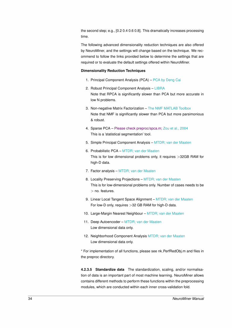
the second step; e.g., [0.2 0.4 0.6 0.8]. This dramatically increases processing
time.
The following advanced dimensionality reduction techniques are also offered
by NeuroMiner, and the settings will change based on the technique. We rec-
ommend to follow the links provided below to determine the settings that are
required or to evaluate the default settings offered within NeuroMiner.
Dimensionality Reduction Techniques
1. Principal Component Analysis (PCA) – PCA by Deng Cai
2. Robust Principal Component Analysis – LIBRA
Note that RPCA is significantly slower than PCA but more accurate in
low N problems.
3. Non-negative Matrix Factorization – The NMF MATLAB Toolbox
Note that NMF is significantly slower than PCA but more parsimonious
& robust.
4. Sparse PCA – Please check preproc/spca.m; Zou et al., 2004
This is a ’statistical segmentation’ tool.
5. Simple Principal Component Analysis – MTDR; van der Maaten
6. Probabilistic PCA – MTDR; van der Maaten
This is for low dimensional problems only, it requires >32GB RAM for
high-D data.
7. Factor analysis – MTDR; van der Maaten
8. Locality Preserving Projections – MTDR; van der Maaten
This is for low-dimensional problems only. Number of cases needs to be
> no. features.
9. Linear Local Tangent Space Alignment – MTDR; van der Maaten
For low-D only, requires >32 GB RAM for high-D data.
10. Large-Margin Nearest Neighbour – MTDR; van der Maaten
11. Deep Autoencoder – MTDR; van der Maaten
Low dimensional data only.
12. Neighborhood Component Analysis MTDR; van der Maaten
Low dimensional data only.
* For implementation of all functions, please see nk PerfRedObj.m and files in
the preproc directory.
4.2.3.5 Standardize data The standardization, scaling, and/or normalisa-
tion of data is an important part of most machine learning. NeuroMiner allows
contains different methods to perform these functions within the preprocessing
modules, which are conducted within each inner cross-validation fold.
34 NeuroMiner Manual

Standardization is conducted on each of the features that have been entered
to NeuroMiner across observations. Currently, it calculates the Z-score (i.e.,
(score - mean) / standard deviation) for each feature based on either the entire
sample or a specified subgroup of individuals. The user then has the option to
also apply the calculations to either the full sample or a subgroup.
When option 3 is selected, the user will see the following:
1 : Compute mean & SD from a specific subgroup of cases [ no ]
2 : Apply mean & SD to a specific subgroup of cases [ no ]
3 : Winsorize data (clamping of outliers) [ no ]
4 : Zero-out completely non-finite features [ yes ]
The first two options give the user the option to calculate the mean and stan-
dard deviation from a subgroup of individuals (e.g., controls) and to also either
create Z-scores using these values for all individuals in the group (e.g., pa-
tients and controls) or to apply them to a specific subgroup (e.g., controls or
patients).
The user also has the option to Winsorize or ’censor’ the data. This technique
was introduced to account for outliers. After standardization, the elements
which are outside of a user-defined range (e.g., 4 standard deviations) are set
to their closest percentile. For example, data above the 95th percentile is set
to the value of the 95th percentile. The feature is then re-centered using the
new censored values.
If there are entries in the user’s feature data that are non-numeric (i.e., ”NaN”
or ”not a number” elements), then these will not be considered during the cal-
culation of the mean and standard deviation (NeuroMiner uses the nanmean
function). However, after the data has been standardized, these values will
be added back to the feature matrix. As such, NeuroMiner gives the option to
change these to zero in step four. It is important to note that once the data
has been standardized, zero values reflect the mean of the feature and are
thus a form of mean imputation. If the user wants to use other imputation op-
tions, they can select ’no’ to this option and then impute the data using the
preprocessing imputation option.
4.2.3.6 Scale data Another option to put the data into the same space is to
scale it between two values. The user will see the following menu when they
select this option:
1: Scale across features or each feature independently [each feature indepen-
dently]
2: Define scale range [0,1]
3: Zero-out completely non-finite features [yes]
Using option 1, scaling can be conducted for ”each feature independently” or
”across the entire matrix”. If each feature independently is selected, then the
data will be scaled within the desired range for each feature (i.e., each voxel
NeuroMiner Manual 35

or each questionnaire). If the entire matrix is selected then each value in the
matrix will be scaled according to the range of all the data (e.g., all voxels or
all questionnaires).
The user then has the option to define the scale range between 0 and 1 or
between -1 to 1. These two options are provided because some machine
learning algorithms require the data to be scaled differently; e.g., the liblinear
options require the data to be scaled between -1 to 1.
Non-numeric values are not taken into account during scaling and are added
back to the matrix after scaling. The third option gives the user the ability to
either change these values to zero following scaling by selecting ”yes” for the
third option to ”zero-out completely non-finite features”. It is critical to note that
in this case the values will be considered to be the absolute minimum of the
scale for future analyses (e.g., if IQ is scaled, then these individuals will have
an IQ value of 0). For questionnaire data, it is recommended that this option is
changed to ”no”, and instead imputation is performed after scaling for the NaN
elements. Alternatively, for imaging data, it is recommended that NaN values
are excluded by using a brainmask during data input.
4.2.3.7 Normalize to group mean This option is only available when a
group has been entered as a covariate at the start of the analysis (i.e., dummy
coded vector containing ones for the group and zeros for the other partici-
pants). The option will then normalise all subjects to the mean of the specified
group.
4.2.3.8 Normalize to unit vector This option takes the mean of the data,
then subtracts this from each of the scores within the data. It then calculates
the norm (L1 or L2) of this result. It then mean-centers the original data and
divides each score by the normalised scores.
4.2.3.9 Apply binning method to data Binning is a technique that can be
used to control for variance in data (wiki). For example, a histogram is an
example of data binning. A form of it is discretization of continuous features
(wiki) and this is offered in NeuroMiner as the default option when binning is
selected as follows:
1 : Select binning method [ discretize ]
2 : Define binning start value [ 0 ]
3 : Define binning stepping [ 0.5 ]
4 : Define binning stop value [ 4 ]
Discretization basically just forms bins based on the standard deviation. You
first establish a vector using a start value, a stepping value, and a stop value
called alpha (e.g., the default setting is [0 0.5 1 1.5 2 2.5 3 3.5 4]). It then
discretizes each feature by the mean +/- alpha*std. For example, for the first
value of alpha, it finds the feature values that are above and below the mean
36 NeuroMiner Manual

and gives them a new value (i.e., 1 or -1). Then in the next step it finds the
values that are above and below the mean +/- half of the standard deviation
and gives them a new value (i.e., 2 or -2). In the next step it finds values that
are above and below one standard deviation from the mean and gives them a
new value (i.e., 3 or -3). And so on. In this way, bins are created with a width
that is determined by the standard deviation. It is important to note that this
function will perform Winsorization (i.e., clamping) because values the stop
value of alpha (e.g., above 4 standard deviations above or below the mean)
will be given the final value.
Manually determining the bins is a good way to discretize data if you have a
firm idea about the problem, but if you do not then it is useful to find an optimal
bin width for a feature by taking into account the information content of the data.
This can be done in NeuroMiner by changing the ”1: Select binning method”
to ”Unsupervised entropy-based symbolization”. It tries to find an optimal bin
width for a feature by taking into account the entropy. It will do this within the
range that you specify in the following settings:
1 : Select binning method [ symbolize ]
2 : Define minimum bin count [ 3 ]
3 : Define maximum bin count [ 25 ]
4 : Define sequence length [ 4 ]
5 : Define width of data range in number of STDs from mean [ 3 ]
4.2.3.10 Impute missing values The machine learning algorithms in-
cluded in NeuroMiner are not able to process missing values (represented
in MATLAB as ”Not a Number” (NaN) entries). This means that they have
to be either removed using the ”Prune non-informative columns” feature de-
scribed below, or they need to be imputed using this module.
NeuroMiner performs imputation using either single-subject median replace-
ment, feature-wise mean replacement, or multivariate distance-based nearest-
neighbor median imputation. When this feature is selected it will reveal the
following menu:
1 : Define imputation method [ kNN imputation (EUCLIDEAN) ]
2 : Select features for imputation [ All features ]
3 : Define number of nearest neighbors [ 7 nearest neighbors ]
1: Define imputation method
You have to first define the imputation method using the following menu:
1 : Median of non-NaN values in given case
2 : Mean of non-NaN values in given feature
3 : MANHATTAN distance-based nearest-neighbor search
4 : EUCLIDEAN distance-based nearest-neighbor search
5 : SEUCLIDEAN distance-based nearest-neighbor search
6 : COSINE similarity-based nearest-neighbor search
NeuroMiner Manual 37

7 : HAMMING distance-based nearest-neighbor search
8 : JACCARD distance-based nearest-neighbor search
9 : Nearest-neighbor imputation using hybrid method
For median or mean replacement, values are imputed based on the data ei-
ther across features for one subject or across subjects within the feature. For
multivariate nearest-neighbor imputation, for each case with NaN values, a
multivariate statistical technique is conducted to identify a number of similar
(i.e., nearest-neighbor) cases from all the subjects that are available. For ex-
ample, the Euclidean distance could be used to identify the 7 nearest-neighbor
subjects that are close to the subject with the NaN value. Once these similar
cases are identified in the multivariate space, then NeuroMiner will take the
median of their values of the feature with the missing NaN case and impute
it into the NaN field. A number of distance metrics can be used to represent
the cases in multivariate space and to determine the nearest-neighbors based
on the type of data you have (e.g., Manhattan, Euclidean, Seuclidean, Cosine,
Hamming, or Jaccard). For example, the Euclidean distance could be used for
data with a continuous measurement scale or the Hamming could be used for
binary nominal data (i.e., 0 or 1) data (see Box: Nominal Data). There is also
the option to use a hybrid approach that accounts for both continuous/ordinal
and nominal data. It’s important to note that all options except for the Man-
hattan and Euclidean distances require the Statistics and Machine Learning
Toolbox of MATLAB.
1: Median of non-NaN values in given case
This function checks NaN values for each subject. When it finds a NaN value
for a subject, it imputes the median of the non-NaN values across the other
features for that subject. Therefore, this would make no sense at all if it was
done across features that weren’t equivalent in scale or from the same scale
(e.g., a questionnaire). As such, it could be used in combination with the option
to ”2: Select features for imputation” described below.
2: Mean of non-NaN values in given feature
This function cycles through each feature and if it finds a NaN value then it
imputes the mean of non-NaN values.
3: MANHATTAN distance-based nearest-neighbor search
This function determines the Manhattan distance between cases and then se-
lects nearest-neighbors. It uses the ’distance’ function from the Large Margins
Nearest-Neighbors (LMNN) toolbox version 2.5 (link). You must scale, unit-
normalize or standardize the data first, otherwise the distance measure will be
dominated by high-variance features.
4: EUCLIDEAN distance-based nearest-neighbor search
Determines the Euclidean distance between cases and then selects nearest-
neighbors. It uses the ’distance2’ function from the Large Margins Nearest-
Neighbors (LMNN) toolbox version 2.5 (link). You must scale, unit-normalize
or standardize the data first, otherwise the distance measure will be dominated
38 NeuroMiner Manual

by high-variance features.
5: SEUCLIDEAN distance-based nearest-neighbor search
The Seuclidean distance between cases is measured using the pdist2 function
that is built into the Statistics and Machine Learning Toolbox of MATLAB.
6 : COSINE similarity-based nearest-neighbor search
The Cosine distance between cases is measured using the pdist2 function that
is built into the Statistics and Machine Learning Toolbox of MATLAB.
7 : HAMMING distance-based nearest-neighbor search
The Hamming distance between cases can be used for nominal data (e.g., 0/1
data) and is measured using the pdist2 function that is built into the Statistics
and Machine Learning Toolbox of MATLAB.
8 : JACCARD distance-based nearest-neighbor search
The Jaccard distance between cases is measured using the pdist2 function
that is built into the Statistics and Machine Learning Toolbox of MATLAB.
9 : Nearest-neighbor imputation using hybrid method
This option combines techniques that can be used for binary nominal data
(i.e., 0/1) and ordinal/continuous data. You must define a method for nomi-
nal features (e.g., Hamming or Jaccard) and then define a method for ordi-
nal/continuous features (e.g., Euclidean or Cosine). The maximum number of
unique values for nominal feature imputation must also be inputted.
Box: Nominal Data.It is important to remember that nominal data with more
than two categories needs to be dummy-coded for the results to make sense
(i.e., 0 or 1 coding). NeuroMiner does not recognise the data-types and there-
fore nominal data that is coded with more than three categories (e.g., 1=De-
pression; 2=Bipolar; 3=Schizophrenia) will be used as a variable with mean-
ingful relationships between the numbers when the differences are actually
arbitrary.
2: Select features for imputation
The imputation procedures can be applied to the entire dataset or to subsets
of the data. This is useful when there are different data domains (e.g., clinical
and cognitive data) or even single questionnaires (e.g., the PANSS) that you
want to restrict the imputation to. A MATLAB logical vector (i.e., consisting
of TRUE and FALSE fields that are depicted as [0 0 0 1 1 0 0 etc.]; you can
convert a binary vector to a logical simply by typing logical(yourvector) on the
command line) must be provided to select a subset. If you want to impute
multiple subsets then you must add separate imputation routines.
3: Define number of nearest-neighbors
If you’re using the multivariate nearest-neighbors approach then you must de-
fine the number of nearest neighbors (e.g., subjects) to use for the calculation
of the median value. The default is 7.
NeuroMiner Manual 39

4.2.3.11 Prune non-informative columns from data matrix Data pruning
is the removal of examples or features that will not work with machine learning
algorithms or are redundant. In NeuroMiner, the machine learning algorithms
that are used cannot work with missing values (i.e., ”Not a Number” (NaN) en-
tries in MATLAB) or with infinite values (i.e., ”Inf” in MATLAB), which can occur
due to previous processing steps. If the values of a feature do not change be-
tween participants (i.e., there is zero variance), then it is redundant to include
the feature in the analysis as well. To correct for these problems, NeuroMiner
offers the following options:
1 : Prune zero features [ no ]
2 : Prune features with NaNs [ yes ]
3 : Prune features with Infs [ yes ]
4 : Prune features with single-value percentage over cutoff [ yes, 5 ]
The first option gives the user the ability to remove variables with no variance
within a fold (i.e., if all individuals, or ’examples’ within a cross-validation fold
have exactly the same value for a feature).
The second option will remove features within a fold that have any NaN (’Not a
Number’) values. Similarly, the third option will allow users to remove features
with any Infs (Infinity) values.
It is important to note that even if there is one subject with one NaN or Inf within→ Be careful with pruning
the fold NeuroMiner will remove the feature. The amount of removed features
will be difficult to quantify. For matrix data, check the NaNs and potentially filter
then prior to the entry into NeuroMiner (see 4).
The fourth option is used in situations where there are a large number of sub-
jects with the same value and a few with different values. For example, in
neuroimaging due to registration inaccuracies most of the subjects may have a
voxel value of zero in a location close to the gray matter border and a few might
have non-zero numbers. In these circumstances, you might want to exclude
the voxels where there is no variance in, for example, 90% of the sample (e.g.,
where 90% of individuals have a zero value). You can specify a percentage
here to do this.
4.2.3.12 Rank / Weight features Selecting or ranking features is an impor-
tant part of machine learning and can be achieved with filters and wrappers.
For a discussion of why these methods are important and for all definitions see
Guyon et al., 2003. Wrappers will be discussed in section 4.2.6 of the manual,
whereas filters are outlined here and also in section 4.2.6.
Filter methods broadly involve the weighting and ranking of variables, and op-
tionally the selection of top performing variables. This can be conducted either
prior to the evaluation of the model during pre-processing or as part of model
optimisation (discussed in section 4.2.6). This option allows the user to weight
variables in the training folds based on some criteria (e.g., Pearson’s correla-
40 NeuroMiner Manual

tion coefficient with the target variable) and then rank them in a specified order
(e.g., descending order from most to least correlated). When this option is
selected, the following will be displayed:
1: Define target labels [ NM target label ]
2: Choose algorithm and specify its parameters [Pearson’s]
3: Up- or down-weight predictive features [ upweight features ]
1: Define target labels
Here the user defines the target label that the filter will be applied to using
the original data; e.g., this could be your group labels if you have a classifica-
tion problem or your questionnaire item if you’re using regression. The default
setting in NeuroMiner is to use your target variable, but this van be changed
by first selecting the menu item and then entering ”D” to define a new target
label. A new menu will appear and you can select to enter either categorical
or continuous data. You can then enter a MATLAB vector that defines either
categorical labels (e.g., [0 0 0 0 1 1 1 1]) or continuous labels (e.g., [15 26 19
33 22]). These variables should be stored in your MATLAB workspace.
When a continuous variable is selected, the user will then be asked whether
they want to weight feature using only one specific subgroup. This means that
the feature will only be weighted only based on the relationship between the
feature and the filter target in one subgroup (e.g., control participants).
2: Choose algorithm and specify its parameters
The user here has the option to choose from among a number of methods that
will weight the relationship between the filter target and the feature. These are:
1: Pearson / Spearman correlation
Standard MATLAB functions for Pearson’s (corrcoef).
2: Spearman correlation
Standard MATLAB function for Spearman’s (corr).
3: G-flip (Greedy Feature Flip)
See Gilad-Bachrach et al. (2004) and site
4: Simba
See Gilad-Bachrach et al. (2004) and site
5: IMRelief
This is an implementation of the Yijun Sun IMRelief function called ”IMRelief
Sigmoid FastImplentation” (see Sun & Li, 2007).
6: Relief for classification
This is a version of the built-in MATLAB ReliefF algorithm (link).
7: Linear SVC (LIBSVM)
This weights the features by conducting a linear SVM using each independent
feature, as implemented in LIBSVM (Chang & Lin).
NeuroMiner Manual 41

8: Linear SVC (LIBLINEAR)
Weights the features based on using LIBLINEAR toolbox (link)
9: F-Score
Weights the features based on conducting an ANOVA using standard MATLAB
functions on the differences between the groups when problem is classification.
10: AUC
Calculates an area under the curve (AUC) for binary classifications based on
the code of Chih-Jen Lin and then ranks the features based on this.
11: FEAST
Implementation of the FEAST toolbox for feature selection (site).
12: ANOVA
Standard implementation of ANOVA.
13: External ranking
This option uses a user-defined weighting template that was entered during
data input (see 4.1), to use an external weighting map from a file, or to read-in
a weighting vector using the MATLAB workspace.
3: Up- or down-weight predictive features
This option allows the user to either upweight or downweight the features
based on the relationship between the variable and the target. For example, if
you want to increase the importance of the features based on the target you
would upweight the features. If you want to reduce the importance of the fea-
tures based on some other variable (e.g., age if it is a nuisance variable) you
could select the variable as the feature selection target and then choose the
downweight option. For more information about why you would want to do this
see references above.
4.2.3.13 Correct group offsets from global group mean This function
was introduced primarily to control for scanner differences in structural neu-
roimaging data. In the case of two centers, for each feature, the mean of both
center A and center B is calculated. The mean difference between these is
then calculated (A-B=Y) and then subtracted from each of the data points in A
(i.e., Ai - Y). This value is stored for further analysis. Internal empirical tests
indicate that this basic method can control for major site differences.
4.2.3.14 Extract variance components from data This function takes a
source matrix and performs a PCA. It then determines correlations between
the eigenvariates from the PCA reduction, and those above or below a spec-
ified threshold are identified. It then projects the target matrix to the source
matrix PCA space, and then back-reconstructs this to the original input space
without the identified PCA components (i.e., it removes the variance associ-
ated with those components).
42 NeuroMiner Manual

4.2.4 Classification algorithm
Support Vector methodologies are the base of the evaluation core of Neu-
roMiner, other methods such as k-Nearest Neighbors and Random Forests
are also available. In this distribution we rely on the LIBSVM /LIBLINEAR
toolboxes for the implementation of support vector based classifiers and re-
gressors. matLearn is also now introduced and requires the Statistics and
Optimization Toolbox.
NeuroMiner interface will change according to the evaluation type selected in
the data input process, two operation modes are implemented: Classification
and Regression. The following will refer to each of these separately.
4.2.4.1 Classification mode In this section we will describe the set up of
Classifiers in Neurominer.
4.2.4.1.1 Define prediction performance criterion During machine learn-
ing, models will be optimised and evaluated based on a criterion. For classifi-
cation problems NeuroMiner provides the following performances measures:
1. Accuracy: sum(E =P)*100/N ACC
2. Matthews Correlation Coefficient: (TP*TN-FP*FN)/sqrt((TP+FP)*(TP+FN)*(TN+FP)*(TN+FN))
MCC
3. Area-Under-the-Curve ROC
4. Balanced Accuracy: (sensitivity+specificity) / 2) BAC
5. Enhanced Balanced Accuracy: (sensitivity*specificity)/100)
6. Prognostic Summary Index: PPV+NPV-100
Notes: E, expected; P, predicted; TP, true positive; TN, true negative; FP, false
positive; FN, false negative; PPV, positive predictive value; NPV, negative pre-
dictive value.
Each of these performance measures can have an effect on the resulting
model and is dependent on the analysis that is being conducted. For example,
simple accuracy is useful when it doesn’t matter if sensitivity and specificity
needs to be balanced (e.g., if sensitivity could be very high and specificity very
low). However, if there are unequal sample sizes then this can lead to very
unbalanced sensitivity and specificity that is an artifact of sample size, which
can be corrected by using balanced accuracy (BAC).
4.2.4.1.2 Configure learning algorithm Learning algorithm to be used for
the classification analysis. Each algorithm has a particular set of parame-
ters that are described in the respective distributions. In general defaults are
provided.
1. SVM – LIBSVM
NeuroMiner Manual 43
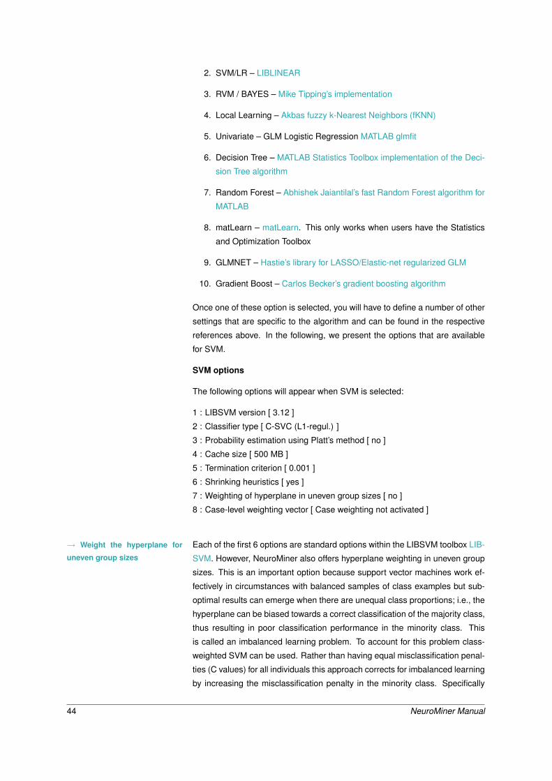
2. SVM/LR – LIBLINEAR
3. RVM / BAYES – Mike Tipping’s implementation
4. Local Learning – Akbas fuzzy k-Nearest Neighbors (fKNN)
5. Univariate – GLM Logistic Regression MATLAB glmfit
6. Decision Tree – MATLAB Statistics Toolbox implementation of the Deci-
sion Tree algorithm
7. Random Forest – Abhishek Jaiantilal’s fast Random Forest algorithm for
MATLAB
8. matLearn – matLearn. This only works when users have the Statistics
and Optimization Toolbox
9. GLMNET – Hastie’s library for LASSO/Elastic-net regularized GLM
10. Gradient Boost – Carlos Becker’s gradient boosting algorithm
Once one of these option is selected, you will have to define a number of other
settings that are specific to the algorithm and can be found in the respective
references above. In the following, we present the options that are available
for SVM.
SVM options
The following options will appear when SVM is selected:
1 : LIBSVM version [ 3.12 ]
2 : Classifier type [ C-SVC (L1-regul.) ]
3 : Probability estimation using Platt’s method [ no ]
4 : Cache size [ 500 MB ]
5 : Termination criterion [ 0.001 ]
6 : Shrinking heuristics [ yes ]
7 : Weighting of hyperplane in uneven group sizes [ no ]
8 : Case-level weighting vector [ Case weighting not activated ]
Each of the first 6 options are standard options within the LIBSVM toolbox LIB-→ Weight the hyperplane for
uneven group sizes SVM. However, NeuroMiner also offers hyperplane weighting in uneven group
sizes. This is an important option because support vector machines work ef-
fectively in circumstances with balanced samples of class examples but sub-
optimal results can emerge when there are unequal class proportions; i.e., the
hyperplane can be biased towards a correct classification of the majority class,
thus resulting in poor classification performance in the minority class. This
is called an imbalanced learning problem. To account for this problem class-
weighted SVM can be used. Rather than having equal misclassification penal-
ties (C values) for all individuals this approach corrects for imbalanced learning
by increasing the misclassification penalty in the minority class. Specifically
44 NeuroMiner Manual

each C parameter for each class is multiplied by the inverse ratio of the train-
ing class sizes. To optimise the serach for optimal class weights, you can
also introduce an additional hyperparameter that multiplies the inverse ratio by
a scaling factor for each class prior to the multiplication of the C parameter.
This can be defined when the learning algorithm parameters settings in sec-
tion 4.2.5. Similarly, option 8 allows you to weight the hyperplane based on a
vector of weighting parameters that you have defined. This will work similarly
to the above, but it will use the parameters entered rather than the group sizes.
Once these options are selected, NeuroMiner will progress to the next menu
to define the kernel type.
4.2.4.1.3 Define kernel type Define whether the algorithm will use a linear
or non-linear kernel Kernel. This will display the following options:
1: Linear
2: Polynomial
3: RBF (Gaussian)
4: Sigmoid
Once these settings are defined, then you will be directed back to the main
menu for this section and you can proceed to the main menu and then can
configure the learning algorithm in section 4.2.5.
4.2.4.2 Regression mode If you have defined a regression framework dur-
ing data input (see section 4.1) then a different menu will appear as follows.
4.2.4.2.1 Define prediction performance criterion Performance criteria
play a major roles in model evaluation and optimization, for regression NM
provides 5 performances measures:
1. Mean Squared Error MSE
2. Normalized Root of Mean Squared Deviation NRMSD
3. Squared Correlation Coefficient R2
4. Correlation Coefficient CC
5. Mean Average Error MAERR
4.2.4.2.2 Configure learning algorithm Learning algorithm to be used for
the regression analysis. Each algorithm has a particular set of parameters
that are described in the respective distributions. In general defaults are pro-
vided.
1. SVM – LIBSVM
2. SVM – LIBLINEAR
3. RVM / BAYES – Mike Tipping’s implementation
NeuroMiner Manual 45

4. Multinomial relevance vector regression (MVRVR) (for multiple target la-
bel prediction)
5. Univariate – GLM Linear Regression
4.2.4.2.3 Define kernel type Kernel to be used in the selected regressor
(when applicable).
1. Linear
2. Polynomial
3. RBF (Gaussian)
4. Sigmoid
4.2.5 Learning algorithm parameters
Parameters for a learning algorithm (e.g., an SVM or SVR) change the way
that the model is fitted to the data. A common example is the ”C” or ”slack”
parameter for soft margin SVM that defines the penalty associated with mis-
classifying individuals–i.e., whether the model does not allow any error within
the CV1 folds and very tightly fits the decision boundary, or whether it allows
error in order to improve generalizability. As such, parameters such as these
can greatly affect the model performance and it is common practice in machine
learning to optimise the parameters for your specific problem and data.
NeuroMiner was developed in order to optimise performance across pre-
defined parameter ranges within the nested cross-validation framework using
a gridsearch, which protects against overfitting due to the application of the
trained models to held-out data. Parameter default ranges are provied in
NeuroMiner based on the literature and empirical testing, but we strongly
recommend that the parameters are defined for your study and problem.
As previously stated, NeuroMiner uses a dynamic menu configuration that
changes based on previous input. This is no different for the learning algo-
rithm parameters, whereby the menu options will change based on what you
have selected in the ”Classification algorithm” section.
Here we show an example for a RBF-Gaussian kernel Support Vector Machine
classifier.
1. Define Slack/Regularization parameter(s)
2. Define Kernel parameter(s))
3. Define Weighting exponents
4. Enable regularization of model selection
Model selection regularization option controls the optimization module in Neu-
rominer. When parameter(s) selection is necessary regularization might be
46 NeuroMiner Manual

advisable. If you answer yes to this question the following options will be avail-
able.
1. Criterion for cross-parameter model selection
2. Suboption 1 dependent on (a)
3. Suboption 2 dependent on (a)
4. Specify cross-parameter model selection process. This option controls
the number of models (parameters combination) selected. One optimal
model based on the criteria and regularization defined previously or an
ensemble of the top performing models
4.2.6 Ensemble generation strategies
NeuroMiner automatically works with ensemble learning at the CV2 level
across the CV1 folds of a nested, repeated cross-validation design (see Fig.
5), but it also includes the ability to apply filters and wrappers that optimise
predictions by selecting features within these folds (for more information, see
link and Kolhavi & John).
4.2.6.1 Filter-based ensemble generation NeuroMiner has two methods
of applying filters: 1) as part of the preprocessing of features by pre-selecting
variables based on their relationship to the target (see 4.2.3.12; 2) as an en-
semble method where different variable sets (variable subspaces) can be cho-
sen based on the performance of the machine learning training algorithm. This
latter case is known as constrained feature optimization because the variable
sets are produced based on the performance of an algorithm (e.g., correlation),
the sets are evaluated with the algorithm, and then the models corresponding
to well-performing variable sets are chosen as an ensemble.
The first step is to turn the option to yes specifying the ”train filter methods on
CV1 partitions”. This will generate a menu with the following:
1: Train filter methods on CV1 partitions
2: Use algorithm output scores or label predictions
3: Specify filter type
4: Define minimum number of features to be selected
5: Specify subspace optimization strategy
6: Define target population for computing optimization
7: Define subspace stepping
1: Train filter methods on CV1 partitions Turn constrained feature optimiza-
tion filtering on or off.
2: Use algorithm output scores or label predictions Choose the feature
sets based on majority voting of the predicted labels (hard decision ensem-
ble) or based on an average of the predicted probabilities from the machine
learning algorithm (soft decision ensemble).
NeuroMiner Manual 47

3: Specify filter type Specify what filter will be used to obtain the feature sets.
These methods are the same as in the preprocessing filter outlined in section
4.2.3.12.
4: Define minimum number of features to be selected This gives the op-
tion to define a minimum number of features that are retained when choosing
feature sets.
5: Specify subspace optimization strategy Once the subspaces are defined
and the models are evaluated, this section will define which subspaces/models
are retained. There is the option to retain one model of the best performing
subspace, or an ensemble of models across well-performing subspaces.
1: Subspace with maximum argmax. Argmax (arguments of the maxima) are
the points of the domain of some function at which the function values are max-
imised. This option picks the maximum argmax across the feature subspaces
(winner-takes-all).
2: Subspace ensemble with maximum argmax Picks the X most predictive
subspaces with reference to the argmax.
3: Subspace ensemble with maximum argmax above a percentile Picks the
top X% of subspaces.
4: All-subspace ensemble Uses all subspaces when training the model.
6: Define target population for computing optimization You can choose
the best performing models using the CV1 training data, the CV1 test data,
or the CV1 training & the test data. This means that the subspaces will be
selected on the basis of how they predict the labels in each of these data folds.
Selection based on training and test data is recommended.
7: Define subspace stepping This option defines how the subspaces are
formed. The features are ranked based on the association between them and
the target variable, and then they are divided into subspaces based on blocks
of X% of features; e.g., blocks of 10% of features would divide the data into the
top 10% performing features, then the top 20% of features, then the top 30%
of features, and so on.
It is important to note that once the feature subspaces are defined, the features
within the winning subspaces can then be used in a wrapper to further optimise
performance.
4.2.6.2 Wrapper-based model selection The wrapper methods in Neu-
roMiner use either Greedy feature selection or simulated annealing to select
feature combinations that maximise the predictive accuracy of a model in the
CV1 data. You will see the following menu:
1 : Deactivate wrapper methods
2 : Wrapper type [Greedy feature selection (Use CV1 test data; Stop at k=50%
of features; Cross-CV1 PFE off)]
48 NeuroMiner Manual

3 : CV1 data partitions for optimization [CV1 test data]
4 : Cross-CV1 Feature selection [Cross-CV1 PFE off]
2: Wrapper type Select Greedy feature selection or simulated annealing.
Each option will lead to a new menu as follows:
Greedy Feature Selection
1 : Search direction [ Forward ]
2 : Early stopping [ Stop at 50% of feature pool ]
3 : Feature stepping [ Each feature will be evaluated ]
The search direction must be provided (forward or backward), which deter-
mines whether an empty subspace is filled with features that are the most
predictive of the target variable (forward selection) or whether all the variables
are entered into the subspace and then variables are removed until the optimal
model is found (backward)
Early stopping is when variables are added up to a total percentage of the
feature pool and then no more variables are added. This feature is useful
when you want to find parsimonious solutions and also because restricting the
feature pool can lead to better solutions.
Feature stepping can also be changed from adding/removing single features
and then testing the model, or adding/removing percentages of features before
testing the model. Adding percentages (e.g., 5%) normally results in a faster
processing time.
Simulated Annealing
1 : Sparsity constant [ 0.01 ]
2 : Starting temperature [ 1 ]
3 : Stopping temperature [ 0.005 ]
4 : Alpha [ 0.9 ]
5 : Maximum # of iterations [ 2000 ]
6 : Maximum # of repetitions in Temperature T [ 100 ]
7 : Minimum # of repetitions until solution is accepted in T [ 30 ]
8 : k constant (smaller k ==> less solutions accepted) [ 10 ]
Simulated annealing is a probabilistic technique for approximating the global
maximum of a function wiki. The settings are standard parameters for any
simulated annealing analysis.
3: CV1 data partitions for optimization Choose either the CV1 training, test,
or test & training data to optimize the feature set.
4: Cross-CV1 feature selection In a nested cross-validation design, you will
have a selection of features for each of the CV1 partitions. This step allows
you to select features across the CV1 folds and will reveal another menu:
1 : Optimize feature selection across CV1 partitions [ yes ]
2 : Probabilistic feature extraction mode [ % Cross-CV1 feature selection
agreement ]
NeuroMiner Manual 49

3 : Apply consistency-based ranking to [ Prune unselected features from each
model and retrain models ]
Probabilistic feature extraction
1 : % Cross-CV1 feature selection agreement
2 : Absolute number of most consistently selected features
3 : Percentage of most consistently selected features
The first option allows you to select features that occur across CV1 partitions
at a certain percentage rate. For example, select only features that appear
across CV1 folds 75% of the time or above this. Sometimes the threshold
that is set does not return any features, and therefore you will also be asked to
define a tolerance value for this circumstance. For example, if the 75% criterion
is not met, then reduce this by 25% (i.e., so then you are effectively selecting
features 50% of the time). You will also be asked to define a minimum number
of features that must be selected each time (e.g., 1 feature).
Option 2, ”Absolute number of most consistently selected features”, just orders
the features based on the amount of times they were selected across the CV1
folds. Then you can select however many features that occur at the top of the
list (e.g., you could select the top 10 most consistently selected features).
Option 3, ”Percentage of most consistently selected features”. This option
sorts in the same way as described for absolute number of consistently se-
lected features and then establishes a cut-off. The features above this cut-off
are kept. For example, if 90% is the cut-off then it will select the top 10% most
consistently selected features across the CV1 folds.
Apply consistency-based ranking
1 : Retrain all CV1 models after pruning them from unselected features
2 : Retrain all CV1 models using the same selected feature space
Once the features are selected, you can either ”1: Retrain all CV1 models” after
pruning the unselected features. Or you can completely retrain the models
using the single optimized feature set that was found in the previous steps.
4.2.7 Visualization options
In NeuroMiner, visualization refers to the representation of the model weights
for each feature. In the case of neuroimaging, this means that the brain maps
are ’visualized’. This setting gives the user the option to derive Z scores and P
values using permutation analysis.
The magnitude of the feature weights do not necessarily inform the user
about the statistical significance (i.e., the degree to which the result may repli-
cate)(see Bilwaj & Davatsikos, 2013). To do this, permutations analysis can
be conducted to create an empirical null distribution of weights for each fea-
ture and then the observed weight is compared to this distribution. This is
described in the supplementary material of Koutsouleris et al. (2016).
50 NeuroMiner Manual

The method is based on Golland & Fischl (2003) and involves the permutation
of the outcome labels, features, or both. For each permutation, the models are
retrained in the cross-validation framework using the respective feature/label
subsets obtained from the observed-label analyses. For each permutation, the
predictions are accumulated of the random models into a permuted ensem-
ble prediction for each CV2 subject. Thus, a null distribution of out-of-training
classification performance (BAC) for the prediction models is constructed. The
significance of the observed out-of-training BAC is calculated as the number
of events where the permuted out-of-training BAC is higher or equal to the
observed BAC divided by the number of permutations performed. The sig-
nificance of the model can then be determined by using a p threshold (e.g.,
p>0.05).
When the option is selected, you will be prompted to enter the number of per-
mutations conducted (this will be dependent on sample size, analysis com-
plexity, and computational time) and then whether you would like to have the
labels, the features, or both permuted (see Golland et al., 2003 for details).
It is important to note that using PCA with this method will result in overly
conservative p-values and is not recommended.
4.2.8 Model saving options
This option will save all the models used in training and testing. This is gener-
ally not a good idea because it will take up too much space.
4.2.9 Save parameter template
Once the parameters are defined in the above steps, they will be included
within the ”NM” MATLAB structure and will be ready to be ”initialised” in the
previous menu. However, the user also has the option here of saving the
parameter settings into a separate .mat file so that they could re-load them for
another analysis. This allows the user to be certain that the same parameters
are applied in analyses with different data.
Please note when saving that loading parameter templates from different ver-
sions of NeuroMiner is currently unsupported.
4.2.10 Load training template
When a parameter template has been saved in the previous menu item, it can
be loaded with this feature. This will parametise all settings within the template
of the new NM structure, and thus will allow it to be initialised in the next step.
Please note that you will see a menu item warning about the cross-validation
set-up. This warning is to highlight the fact that if you have different data then
you need to re-create the cross-validation structure.
NeuroMiner Manual 51

4.2.11 Define verbosity level
During preprocessing, this option will either output all processing steps being
performed on the data using the ”detailed” setting (recommended for first time
use and to check processes) or you can set it so that it only outputs the training
fold that it’s working on and nothing else (the ”none” setting). Setting this to
”none” will increase the speed of analysis because it will not have to print the
steps to screen.
4.3 Multi-group analyses
Multi-group analysis is a more advanced feature of NeuroMiner where clas-
sification is used to distinguish between subjects from multiple groups (e.g.,
schizophrenia, bipolar, and depression subjects). During data input, these
groups are simply defined within the labels–e.g., ’SCZ’, ’BP’, and ’DEP’ identi-
fiers. Once this is defined, then an option will appear in the parameter template
called ”Multi-class settings”. Selecting this option and then selecting the option
to ”Train multi-class predictor” to ’yes’ will reveal another option to ”3 : Specify
multi-class decision mechanism [ ]”. This option determines how NeuroMiner
deals with the multiple groups (e.g., how it optimises the predictions) and is
critical for the interpretation of results. For all the methods included here, it is
important to note that NeuroMiner works by conducting multiple binary analy-
ses between each group pair (see Aly, 2005 for an overview of the main types
introduced below).
Selecting this option will reveal the following menu:
1 : Simple Pairwise Decoding (Maximum-Wins method)
2 : Error-correcting output codes
3 : Hierarchical One-vs-One method
Simple pairwise decoding This is the simplest method. Given that Neu-
roMiner has conducted different pair-wise classifications between all the group
pairs, this option will categorise the individual by their maximum score across
all the classifiers. For example, in a three group problem, if an individual’s score
is highest for the schizophrenia group in the comparison between schizophre-
nia and bipolar (i.e., as opposed to the SCZ-BP, or SCZ-DEP, or BP-DEP) then
they will be classified in the schizophrenia group.
Error-correcting output codes Error-correcting output codes (ECOC) is a
meta-method that is used to solve multi-group classification problems that ap-
plies a voting scheme (i.e., an ensemble method) to decide upon the correct
class. It works by assigning a binary code to each group and then binary
functions are learned one for each bit position in the binary code strings (see
Dietterich et al., 1995 and Dietterich and Bakiri, 1991 and Kinderman et al.
and for an overview see Aly, 2005). Optimal results are obtained by maximally
separating the codes using a distance metric, such as the Hamming distance.
52 NeuroMiner Manual

Hierarchical One-vs-One Method This technique arranges the classes into a
tree and then at each node of the tree a binary classifier makes the discrim-
ination between the different child class clusters (see Aly, 2005 and Wang et
al., 2009).
4.4 Stacking
Stacking is an advanced feature of NeuroMiner that takes multiple learned
decision values, combines them, and then learns again from this meta-
information (see wiki). This technique has provided better solutions than
using single models to learn the classification or regression problem. Stacking
can be done in NeuroMiner if you have different data modalities (e.g., you can
learn from clinical and neuroimaging separately and then stack the learners)
or if you have run separate analyses on one (or more) modalities (e.g., if you
run a linear SVM and then a non-linear SVM and then combine the learned
models).
If you have more than one modality or have run separate analyses on the
same data, then an option will appear in the ”Define parameter template” menu
entitled ”1: Define meta-learning/stacking options”.
1 : Activating stacking using prediction generated by other analyses [ ]
2 : Select 1st-level analyses to provide features to stacker [ selected: ]
3 : Define feature names [ ] 4 : Extract predictions from ...
1: Activating stacking using prediction generated by other analyses Turn
stacking on or off.
2 : Select 1st-level analyses to provide features to stacker Of the analyses
that have been conducted, select the models that you want to stack.
3 : Define feature names [ Var ’feats’] Optionally define feature names for
each of the models that you want to stack.
4 : Extract predictions from ... This gives the option to extract predictions
from either the CV1 training data or the CV1 test data (the default). If CV1
test data is used, the higher-level algorithms should not be combined with
wrappers because of overfitting. Cross-CV probabilistic feature extraction is
helpful in this regard to prevent overfitting.
Once stacking is turned on and these options are defined, then all parameter
settings now relate to the stacked models (e.g., all the preprocessing and train-
ing settings). These settings will need to be changed because the data inputs
are now the decision scores for each of the models (i.e., you’ll have to change
the preprocessing accordingly). Then you can return to the main menu, initial-
ize the stacking models, and train as normal. The results will then relate to the
stacked models rather than the original data.
It’s important to note that the results now pertain to the decision scores of
the stacked models and therefore the interpretation of results is based on the
NeuroMiner Manual 53

models and not the original data (i.e., you can see how one model performed
over another, but not information related to the individual variables).
Please note, that stacking does not work with external validation data.
4.5 Initialize analyses
As outlined in section 4, after the machine learning parameters have been de-→ After defining analyses you
must initialise them fined in the parameter template (section 4.2) then you have to initialize them for
further analysis using the initialisation manager. If analyses in the parameter
template are changed, you must also re-initialise them using this menu. You
can initialise and change as many analyses as you like.
When an analysis is first initialised, a directory will be created containing de-
tails and parameters of the analysis in a log file (see below). During process-
ing, NeuroMiner will store analysis files in this location for this analysis. These
data reporting features allow you to keep track of analyses and provide a stan-
dardised NeuroMiner output format.
It’s important to note that within NeuroMiner you can initialise one analysis,
then change settings in the parameter template (see 4.2), and then initialize
another analysis. This has two implications: 1) the results from different anal-
yses can be compared; 2) with the results of different classifiers, you can use
the advanced feature called stacked generalization (see 4.4. It is important to
note that simply changing settings in the parameter template does not have
any effect on analyses until you initialise the analyses using this menu. If you
want to change the settings of an analysis then change then in the parameter
template and then reset the initialised analyses using the directions below.
The initialization menu can be split into two parts: 1) when no other analysis
is present; 2) when there are existing analyses. And will result in the outputs
described below.
4.5.1 First Initialization
The following menu will appear:
Define analysis identifier [ ? ]
Provide analysis description [ ? ]
Specify parent directory of the analysis [ ? ]
PROCEED >>>
Define analysis identifier Provide a brief description of the analysis; e.g.,
SVM analysis1. This will be used as an analysis ID and also used as an iden-
tifier for the analysis-specific directory created by NeuroMiner.
Provide analysis description Here you can write a more extended analysis
description; e.g., ”this is a test analysis that was created using the default
settings of NeuroMiner”. You can enter multiple lines if you would like and then
enter a single period (i.e., ”.”) to stop the process and enter the data.
54 NeuroMiner Manual
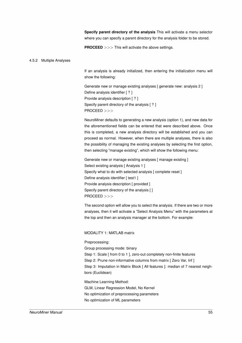
Specify parent directory of the analysis This will activate a menu selector
where you can specify a parent directory for the analysis folder to be stored.
PROCEED >>> This will activate the above settings.
4.5.2 Multiple Analyses
If an analysis is already initialized, then entering the initialization menu will
show the following:
Generate new or manage existing analyses [ generate new: analysis 2 ]
Define analysis identifier [ ? ]
Provide analysis description [ ? ]
Specify parent directory of the analysis [ ? ]
PROCEED >>>
NeuroMiner defaults to generating a new analysis (option 1), and new data for
the aforementioned fields can be entered that were described above. Once
this is completed, a new analysis directory will be established and you can
proceed as normal. However, when there are multiple analyses, there is also
the possibility of managing the existing analyses by selecting the first option,
then selecting ”manage existing”, which will show the following menu:
Generate new or manage existing analyses [ manage existing ]
Select existing analysis [ Analysis 1 ]
Specify what to do with selected analysis [ complete reset ]
Define analysis identifier [ test1 ]
Provide analysis description [ provided ]
Specify parent directory of the analysis [ ]
PROCEED >>>
The second option will allow you to select the analysis. If there are two or more
analyses, then it will activate a ”Select Analysis Menu” with the parameters at
the top and then an analysis manager at the bottom. For example:
MODALITY 1: MATLAB matrix
Preprocessing:
Group processing mode: binary
Step 1: Scale [ from 0 to 1 ], zero-out completely non-finite features
Step 2: Prune non-informative columns from matrix [ Zero Var, Inf ]
Step 3: Imputation in Matrix Block [ All features ]: median of 7 nearest neigh-
bors (Euclidean)
Machine Learning Method:
GLM, Linear Regression Model, No Kernel
No optimization of preprocessing parameters
No optimization of ML parameters
NeuroMiner Manual 55

Cross-Validation:
CV2: 10x10, CV1: 10x10
ANALYSIS MANAGER: CURRENT ANALYSIS: 2 (of 2 ANALYSES)
1 : Select current analysis
2 : Generate new analysis
3 : <= Go to previous analysis
<== Back/Quit [Q]
This menu will give the user the ability to view what has been initialised and to
navigate through the analyses and choose the right one.
Once an analysis has been selected, the user will be returned to the main
menu and can then modify the analysis by selecting the third option to ”Specify
what to do with the analysis”:
1 : delete
2 : completely reset
3 : reset parameters (risk of inconsistency)
Here the user can select the option to delete the analysis, to completely reset
and overwrite all the parameter settings with the new settings in the parameter
template, or to reset parameters. Once an option is selected, you’ll be taken
back to the main analysis manager and you will need to ”PROCEED >>>>”
for the options to take effect.
4.5.3 Outputs and Directory Structure
Once an analysis has been initialised, a folder will be created like the following:
NM ID736740 54131 A1 your-description
This outlines the NM identifier associated with the entered data (e.g., ID736740 54131),
the analysis that has been initialised (e.g., A1 ), and the description that you
entered in the ”Define analysis identifier”.
Within the folder there is a ”params” subfolder and also a log file (e.g.,
”NM Analysis test1.log”). The log file contains an ”NM ANALYSIS LOG FILE”
with a description of the computer and the versions of MATLAB and Neu-
roMiner, in addition to a description of all the analysis parameters that were
conducted. The params subfolder has these details and more specific set-
tings stored in a .mat file containing MATLAB structures that are used by
NeuroMiner.
Following intialization, you can then go to the main menu and preprocess or
train the
4.5.4 Once an Analysis has been Initialized
Once an analysis has been initialised, you can then preprocess the features
and train the models using the directions below. These files will be stored in
56 NeuroMiner Manual

the directory for that analysis.
4.6 Preprocess features
Once the data has been initialized, the user has the option to preprocess the
features. In NeuroMiner nomenclature, this refers to any steps that are con-
ducted within the cross-validation folds prior to training a model. For example,
the data within each fold could be scaled and then imputed, or a principal com-
ponents analysis could be conducted.
When this option is selected, the user will be presented with the following:
1 : Select analysis to operate on [Analysis 1]
2 : Overwrite existing preprocessed data files [ no ]
3 : Use existing preprocessing parameter files, if available [ no ]
4 : Write out computed parameters to disk (may require A LOT of disk space)
[ no ]
5 : Select CV2 partitions to operate on [ 0 selected ]
2: Overwrite existing preprocessed data files. NeuroMiner will save pre-
processed data files and selecting this option will overwrite them.
3: Use existing preprocessing parameter files, if available. The user has
the option to save parameter files (e.g., betas from regression of age from a
feature) and this option will allow them to use the existing files.
4: Write out computer parameters to disk. This option will write the param-
eters (e.g., beta coefficients) to disk. This is not recommended due to space
limitations.
5: Select CV2 partition to operate on. This option will only appear if an
analysis has been selected in step 1. It allows the user to select the folds that
the preprocessing analysis will be applied to (see Box: Selecting CV folds in
NeuroMiner).
NeuroMiner Manual 57

Box: Selecting CV folds in NeuroMiner. Because NeuroMiner was de-
veloped with nested, double cross-validation as the gold standard, there is
an option to only select the outer, CV2, folds that you want to process. For
example, you could select only the first permutation in order to check that
everything is working before running the rest of the permutations.
When the option is selected, the user will see the CV2 cross-validation folds in
a block of permutations and folds:
e.g., Perm 1: * * * * *. A star ”*” indicates that the fold is selected, whereas
the letter ”o” indicates the fold is not selected; e.g., Perm 1: o o o o o. Please
note that all folds are selected by default in NeuroMiner, and thus you would
need to de-select all folds first if you wanted to select specific perms or folds.
The user can select and de-select the folds in single positions or ranges. The
folds can be referenced by first indicating the permutation (e.g., 1st permuta-
tion) and then the fold position (e.g., 1st fold). For example, the second fold
of the first permutation would be [1,2]. A fold range can also be selected in
the following format [perm start, perm end, fold start, fold end]. For example,
you may want to select the first two permutations and the first three folds in the
following way: [1,2,1,3].
4.7 Train supervised classifiers
As depicted in Figure 3, once the parameter template has been completed
and initialized there is the option to train the models. This implies the use
of a statistical technique, such as an SVM, along with the hyperparameter
optimisation (e.g., optimising the C parameter) and any wrappers that might
have been activated. The following menu will be displayed:
1: Create analysis from scratch
2: Create analysis using precomputer preprocdata-MATs
3: Create analysis using precomputed CVdatamats
4: Create analysis using precomputed CVresult-MATs
1: Create analysis from scratch
This is where the analysis has only been initialized and no data matrices have
been stored. This will preprocess and then train classifiers. Please note, that
if your matrices are large (e.g., with neuroimaging data) then this will take up a
lot of RAM and as such it is recommended to preprocess the data first.
2: Create analysis using precomputer preprocdata-MATs
This is when the user has preprocessed their data and stored the preprocessed
files in a folder; i.e., they have TRAIN files.
3: Create analysis using precomputed CVdatamats
This is when the user has completed an analysis (preprocessing and training)
and they have the data matrix files stored in a folder; i.e., ”...CVdatamat oCV...”
files. When this option is selected, the analysis results from the CVdatamat
files are then collated into a result file. It is useful especially when the program
58 NeuroMiner Manual

Figure 6: Monitor progress during an analysis.
has crashed, and/or the NM structure has not been saved, and the user wants
to get the results without re-running all the training again.
4: Create analysis using precomputed CVresult-MATs
This is when the user already has the results file and they want to integrate the
results into the NM structure. This is useful if there has been a crash and the
data has been lost from the NM structure.
4.8 Visualize classifiers
A standard NeuroMiner analysis will produce the predictive accuracy of the
models using the preprocessed data (e.g., the scaled PCA components). This
means that the model weights (e.g., from an SVM) are only available within this
space (e.g., a weight for each PCA component). For accurate interpretation,
it is necessary to project these weights back to the original data and this is
called ”visualisation” within NeuroMiner. The term visualisation applies best to
NeuroImaging data where the weights are projected back to the original voxel
space and then can be visualized, but also applies to matrix data where the
results for each test (e.g., for each questionnaire item) can be visualized in
a graph. Running the visualization routine in NeuroMiner will produce three
different types of results that represent how the classifier relates to the original
data: mean results, grand mean results, and z/p value results.
Mean Results
** Mean **
This image represents the median of the weights across all models selected
during the CV1 cycle. For example, if you have a 10x10 cross-validation cy-
cle and you’re selecting the winner for each fold, then it will create a median
across 100 models.
NeuroMiner Manual 59

** SE **
The standard error of the weights across all models selected during the CV1
cycle.
** CVratio **
This is the sum of the median weights across all CV1 folds divided by the
standard error.
Grand Mean Results
** Mean-GrM **
Within a nested cross-validation framework, the grand median (GrM) in Neu-
roMiner is defined as the sum of the median weights of selected CV1 models
for each CV2 fold, divided by the number of CV2 folds.
** SE-GrM **
The grand median standard error is the sum of the standard error values of
selected CV1 models for each CV2 fold, divided by the number of CV2 folds.
** CVratio-GrM **
The grand median CV ratio is the sum across CV2 folds of the selected CV1
median weights divided by the selected CV1 standard error. This value is then
divided by the number of CV2 folds.
** Mean-gr-SE-GrM **
Across CV2 folds, this is the grand median thresholded to only display the
voxels where the median is greater than the standard error.
** Prob95CI-GrM **
Across CV2 folds, this is the amount of times that the median value has been
greater or less than the 95% confidence interval.
Z and P score images Visualisation can also include the derivation of Z or P
scores using permutation testing. These are outlined in 4.2.7.
4.9 Display training results
Once initialization, preprocessing, and model training has been performed,
the results can then be displayed using this option. The results display inter-
face can be understood in three main divisions: 1) the accuracy and model
performance (initial screen); 2) the model performance across the selected
hyperparameters; 3) results concerning the individual features in the analysis.
60 NeuroMiner Manual

4.9.0.1 Accuracy and Model Performance See Fig. 7. The performance
of a model can be fundamentally described by the degree to which the predic-
tions match the target scores (e.g., how many people are classified correctly or
how closely the features and target are related in a regression). In NeuroMiner,
this is represented in multiple ways that each address a different aspect of the
relationship between subjects, predictions, and targets.
4.9.0.2 Classification Performance See Fig. 8. NeuroMiner was built to
work with hyperparameter optimisation within a nested-cross validation frame-
work as a standard. In this plot, you will see the inner-cycle, CV1, mean test
performance plotted in blue and then the outer cycle, CV2, mean test perfor-
mance plotted in red. Each point represents a hyperparameter combination.
This gives an indication of how the hyperparameter combinations are influenc-
ing the test performance. On the right, the display also shows heatmaps that
show how the performance in the CV1/CV2 folds changes over the permuta-
tions.
4.9.0.3 Generalization Error See Fig. 9. Another way to look at CV2 test
performance is with the generalization error, which is calculated in NeuroMiner
as the CV1-test performance minus the CV2 test performance.
4.9.0.4 Model Complexity See Fig. 10. In NeuroMiner, complexity is de-
fined as the percentage of support vectors divided by the number of subjects
in the tested fold. This feature is useful to determine how varying parameter
combinations may affect the fit of the model.
4.9.0.5 Ensemble Diversity See Fig. 11. This is a measure of Shannon
entropy across CV1 models for each CV2 partition. A higher entropy means
higher disagreement between the CV1 models. This measure is useful be-
cause increased entropy will often result in a better fitting model at the CV2
level. It is useful to note that entropy can be maximised as a performance
criterion in addition to accuracy.
4.9.0.6 Model Selection Frequency See Fig. 12. Within an ensemble
framework, the models that are selected within the inner, CV1, cycle are then
applied to the outer test data. For example, if it is a 10x10 CV1 framework with
a winner-takes-all method of model selection, then 100 models will be applied
to the held-out CV2 test fold. This plot displays the percentage of times that
each parameter combination was selected.
4.9.0.7 Multi-Group Results If a multi-group analysis is conducted then
the results display will change to accommodate the groups. See figure 13.
NeuroMiner Manual 61

Select your analysis Select a plot to view Select your classifier
Select what data to plot
Set the x-axis by entering a workspace variable
Prediction results display
Use “F” buttons to open in figure window
ROC Display
Confusion matrix
Prediction metrics
Pie charts of the pre-test probability of correct classification based on the frequency of targets in each group. The gain after analysis is indicated in black. You can enter a different pre-test probability (e.g., from literature) into the box.
Use “E” buttons to export the data
Figure 7: Option 1: classification plot
Figure 8: Option 2: Cross-validation Performance.
62 NeuroMiner Manual

Figure 9: Option 3: Generalization Error.
Figure 10: Option 4: Model Complexity
NeuroMiner Manual 63

Figure 11: Option 4: Ensemble Diversity
Figure 12: Option 5: Model Selection Frequency
64 NeuroMiner Manual

Figure 13: The multi-group display
NeuroMiner Manual 65

Figure 14: The independent test data dialogue box. 1) Press ”Create New...”;2) Click on the new dataset line; 3) Press ”Add/Modify Data in Dataset.
4.10 Generate master files
Master files of the individual preprocessing or analysis files can be created
using this option.
4.11 Out of Sample Cross-Validation
External, out-of-sample cross-validation (OOCV) is a cornerstone of machine
learning and is required for strong generalizability claims. This usually involves
the application of the trained models used to predict targets in the CV2 data
folds to a separate dataset that has been independently collected.
External validation relies on the trained models being completely separate to
the OOCV data. For this reason, after completing the analysis the user must
first lock analyses and start the NM application mode using the following pro-
cedure.
Once an analysis has been completed, from the MAIN INTERFACE, choose:
8: Lock analyses and start NM application mode.
Then select ”y” to close the model discovery.
The MAIN INTERFACE will then change to include: 1: Load data for model
application. Select this option.
A dialogue box will appear (Fig 14). To enter new data, select ”Create New...”,
then select the created set, and then select ”Add/Modify Data in Dataset”. You
will then be redirected to the command prompt where data can be entered
depending on the input of the discovery data (i.e., if it was NIFTI data then the
user will be directed to enter NIFTI data again). The same procedure applies
that is described in 4.1.
Once the data has been entered, you can return to the main menu and run
the option that says ”Apply classifiers to OOCV data”. At this stage, the
results of this analysis cannot be visualised in the NeuroMiner visualisation
66 NeuroMiner Manual

routines. However, they are located in the NM structure that is included
in the workspace. You will need to exit from NeuroMiner and then go to
NM.analysisX.OOCVX (where ”X” is your analysis number) and then inspect
the fields within this structure for either classification or regression results.
4.12 Load NeuroMiner structure
As outlined in section 4, the NM structure is the core structure that NeuroMiner
uses to store and process data. This option allows the user to load it from a
.mat file.
4.13 Save NeuroMiner structure
This option allows the user to save the NeuroMiner structure (NM) as a .mat
file in a folder of the users choosing. Notably, any changes that are made to
the settings of NeuroMiner during an active session are stored within the NM
structure in the workspace. However, program crashes can lead to the loss
of information. We recommend to save the NM structure at critical points of
the analysis: 1) After data entry; 2) after structure initialization; and 3) after
preprocessing or analysis. This ensures that no data is lost.
4.14 Clear NeuroMiner structure
This option will clear the NeuroMiner structure from the workspace. This will
allow the user to select another structure or enter different data.
4.15 Change Working Directory
NeuroMiner will save files in the directory that it is loaded from. This option
allows the user to change the working directory.
4.16 Open Manual
This feature is currently not functional. Please open the manual normally.
4.17 Utilities
4.17.0.8 1: Compile C++ files for NM This option is currently not func-
tional. If there is a ”mex” error, please navigate to the directory and compile
the function.
4.17.0.9 2: Set root paths of neuroimaging tools (SPM/FreeSurfer) If
you want to process structural MRI (nii) or surface files from FreeSurfer (mgz)
then the paths of these tools need to be established. This option will establish
the paths. If the user does not establish the paths, then the neuroimaging
functions will not be displayed.
NeuroMiner Manual 67

4.17.0.10 Freesurfer: Downsampling, registration to fsaverage & matrix
generation This option will change the dimensions of surface files using dif-
ferent fsaverage resolutions; e.g., fsaverage5 or fsaverage6. This is important
because surface files commonly have very high dimensionality.
68 NeuroMiner Manual

5 Example
For a first-time user, NeuroMiner might be best described using an example.
This section will run through a simple example using structural neuroimaging
data.
5.0.1 Example: Structural NeuroImaging Data
The sample data for this example is open source and can be found in (link).
We processed the data with the Voxel Based Morphometry (VBM) toolbox and
we’re going to use the mwrp1 (grey-matter segmented, realigned, warped,
modulated) images. Each voxel of these images represents the relative vol-
ume of grey matter at any location. The aim of the analysis is to predict who is
an individual with a diagnosis of schizophrenia and who doesn’t have a diag-
nosis purely from the grey matter volumes. Based on previous research, the
hypothesis is that those with schizophrenia will be able to be distinguished with
approximately 70% accuracy.
If the SPM path has been added to NeuroMiner, then the main menu will look
like the following:
1 : Load data for model discovery and cross-validation
2 : Load NeuroMiner structure
3 : Change working directory
4 : Utilities
The first step is to enter the data using the first option, which will display the
following menu:
1 : Define machine learning framework [ classification ]
2 : Select data input format [ nifti ]
3 : Define no. of samples and sample identifiers [ ??? ]
4 : Involve unlabeled cases in the analyses [ no ]
5 : Select space-defining image [ ? ]
6 : Describe data [ ? ]
So, we’re going to leave the machine learning framework as classification be-
cause this is a classification problem, and since we haven’t conducted an SPM
analysis we will also opt to import NIFTI files directly. I’ll then select the third
option to define the number of samples and will define the following:
Number of groups? : 2
Define name of group number 1 : SCZ
Define name of group number 2 : CTRL
I’ve entered the individuals which a schizophrenia diagnosis first because then
the sensitivity accuracy of the analysis will be based on this group rather than
the controls. Once this data is entered, then the menu changes to the following:
1 : Define machine learning framework [ classification ]
NeuroMiner Manual 69

2 : Select data input format [ nifti ]
3 : Modify no. samples [ N=2 ] and sample identifiers [ SCZ, CTRL ]
4 : Involve unlabeled cases in the analyses [ no ]
5 : Select space-defining image [ ? ]
6 : Map image files to samples [ ? ]
7 : Describe data [ ? ]
I don’t want to ”Involve unlabeled cases in the analysis”, so I’ll then select
the space-defining image (i.e., the mask; keep in-mind that the images will be
resliced to this). I’ll either be able to select a region from the WFU PickAtlas
or just use my own mask. For this analysis, I don’t want to select individual
regions, so I’m going to select option 2 and use a pre-prepared ICBM mask in
my templates folder. Then because the template is not completely binary and
there is a transition from 0 to 1 at the border of the brain, I’m going to select a
threshold of 0.5 and then define the regions that are greater than or equal to
this threshold (i.e., >=).
I then select option 6 to ”Map image files to samples” and a file selector box
will appear that is the same as in SPM. At the top of the box, you will see what
the box is for: ”Select nifti for sample 1: SCZ”. To select the images, I could
navigate to the directory on the left and select images, but we recommend to
have a file that stores the absolute paths of each of the images in a separate
text file. This is because it keeps a record of what has been entered, but
mainly because the order of the images is very important for later steps. As an
example, my file looks like this:
/NeuroDiagStor1/COBRE/Data/0040000/mwrp1mprage.nii
/NeuroDiagStor1/COBRE/Data/0040001/mwrp1mprage.nii
/NeuroDiagStor1/COBRE/Data/0040002/mwrp1mprage.nii
...
Once I have this file, I then press the small button on the bottom left called
”Ed” and an editor will appear. Then I paste the files into this editor, first for
the SCZ group and then for the CTRL group. I then go back to the main menu
and enter the global grey matter volumes (or the intracranial volume) with data
that I have loaded into the MATLAB workspace. It is critical that these global
volume data are in the same order as the subjects that I have just entered into
NeuroMiner. If they are in the wrong order then the results of the analysis will
be invalid.
I then go back to the main menu and there will now be an option to ”Inspect
images”. I press this, check that the images have been read correctly and then
enter a few images to visually inspect. In this case, 1:4. This will display the
space-defining mask image as well as the first 4 of my mwrp images. They look
good, so I will then choose ”Describe data” and enter: COBREmwrp1. After
this, I will ”IMPORT” the images and this will lead to reslicing and masking with
the space-defining image (i.e., my ICBM template).
70 NeuroMiner Manual

After the data has been imported, a ”MODALITIES” menu will appear with the
analysis descriptor (i.e., COBREmwrp1) at the top, then some details about
the images. It is important to check that these settings are correct, and the
dimensionality of the images. NeuroMiner automatically reports the number
of features and the percentage of zero/NaN (”not a number”) features. This is
important for later analysis (e.g., if there are NaN features then they probably
need to be excluded. It is also important to note that for this analysis, no
covariates have been found in the NM workspace because they have not been
entered yet.
I want to enter covariates of age and sex, so I will choose option ”5: Add
covariate(s) to NM workspace”. These covariates must be already loaded prior
to entering into NeuroMiner, otherwise you will have to exit the program, load
the covariates, and then enter the program again. After pressing 5, I will then
enter the variable that I’ve previously loaded ”cobre covars” and then name
the covariates ”one-by-one” because there are only two: age and sex. It’s
important to note that these variables will just be entered to the NM structure
and the will not be controlled for these variables until you add this as a
preprocessing step.
So now that my variables are in then I’ll choose ”6: Finish data import for dis-
covery & cross-validation analysis”. This means that the data will be saved in
the NeuroMiner structure and I don’t be able to modify it or add to it again.
NeuroMiner locks the data down like this in order to make sure that latter anal-
yses and organisation, relate to the same dataset. So, now that the data are
in, I’ll be taken to the main NeuroMiner menu where I can set-up my analyses.
1 : Inspect data used for model discovery and cross-validation
2 : Set up NM parameter workspace
3 : Initialize & manage analyses
4 : Preprocess features
5 : Train supervised classifiers
6 : Load NeuroMiner structure
7 : Save NeuroMiner structure
8 : Clear NeuroMiner structure
9 : Change working directory
10 : Utilities
As described in section 4, I will need to first set up a parameter template with
the settings that I want, initialize the analysis, and then run it. For this reason,
I’ll go to ”2: Set up NM parameter workspace” and it will take me to the following
menu (see section 4.2):
1 : Cross-validation settings [ ??? ]
2 : Preprocessing pipeline [ ... ]
3 : Classification algorithm [ ... ]
4 : Learning algorithm parameters [ ... ]
5 : Ensemble generation strategies [ ... ]
NeuroMiner Manual 71

6 : Visualization options [ ... ]
7 : Model saving options [ ??? ]
8 : Save parameter template
9 : Load training template
10 : Define verbosity level [ Detailed output ]
The fields with question marks ”???” need to be completed before the analysis
can be initialized or run, whereas the other sections are pre-set with default
settings. The first thing that I need to do is to set-up cross-validation in step 1.
Pressing this enters the cross-validation menu (see section 4.2.2):
1 : Select cross-validation framework [ (Pooled) cross-validation ]
2 : Define no. of CV2 permutations [ P2 = 10 ]
3 : Define no. of CV2 folds [ K2 = 10 ]
4 : Define no. of CV1 permutations [ P1 = 10 ]
5 : Define no. of CV1 folds [ K1 = 10 ]
6 : Equalize class sizes at the CV1 cycle by undersampling [no]
7 : Build CV2/CV1 structure
8 : Load CV structure
9 : Save CV structure
It’s automatically set-up with repeated, nested, cross-validation, which is the
gold standard cross-validation set-up currently (see Fig. 5). I could change
these settings, but in this case I think they’re great for my sample so I’ll just
choose the option to ”7: Build CV2/CV1 structure”. This will then build the
structure and then I’ll go back to the paramter settings menu by simply pressing
the enter key because here the default option is to quit the menu.
I’ll then enter the pre-processing menu by typing ”2” and hitting enter. This will
show me a few default settings:
=========================
CV-PREPROCESSING PIPELINE
=========================
>> Step 1: Scale [ from 0 to 1 ], zero-out completely non-finite features
Step 2: Prune non-informative columns from matrix [ Zero Var, Nan, Inf ]
And the other settings that I could add are:
1 : Enable spatial operations using Spatial OP Wizard
2 : Add preprocessing step
3 : Remove preprocessing step
4 : Insert preprocessing step
5 : Replace current preprocessing step
6 : Modify current preprocessing step
7 : Next step >>
8 : Change order of preprocessing steps
For this analysis, I don’t want to scale the data first because in previous tests
I found that this introduced some noise in the ventrices and I don’t need to
72 NeuroMiner Manual
prune non-informative columns because I know that there are no NaN or Zero
variance features in the data from when I did the import. So I’ll remove both of
these by pressing ”3” and then ”3” again.
Now that the CV-PREPROCESSING PIPELINE is empty, I’ll add the operations
I want using option ”2: Add preprocessing step” and will see this menu:
1 : Correct data for nuisance covariates using partial correlations
2 : Apply dimensionality reduction method to data
3 : Standardize data
4 : Scale data
5 : Normalize to group mean
6 : Normalize data to unit vector
7 : Apply binning method to data
8 : Prune non-informative columns from data matrix
9 : Rank / Weight features
10 : Correct group offsets from global group mean
11 : Extract variance components from data
Then I’ll add the option to ”Correct data for nuisance covariates” (section
4.2.3.3). I’ll then select option 1 and select both covariates by entering ”1:2”,
and I’ll keep the rest of the default settings so that age and sex will the re-
gressed from the entire sample. After I’ve set these options, I’ll then quit to go
back to the preprocessing menu.
After covarying for nuisance covariates, I now want to perform a dimensionality
reduction so I will select ”2: add preprocessing step” and then ”Apply dimen-
sionality reduction method to data” (section 4.2.3.4). There are a lot of options,
but basically it seems that PCA works well most of the time so I’ll select ”1:
Principal components analysis”. Then I’ll keep all the defaults because these
work well too, and return to the main menu. In this step, if I had have wanted
to optimise over a number of different component reductions, then I could have
defined the energy as 1, returned to the preprocessing menu, added another
step, and then added extracted component subspaces and defined something
like [0.2 0.4 0.6 0.8] to see how the algorithm performs when I retain from 20
to 80% of the energy.
Then I want to add some scaling because I’m going to use an SVM and the
data must be scaled for this and also because it makes the results more inter-
pretable. So I’ll select ”4: Scale data” and again just accept the defaults. Now
the CV PREPROCESSING PIPELINE should include:
=========================
CV-PREPROCESSING PIPELINE
=========================
>> Step 1: Correct for nuisance covariates [age,sex]
Step 2: Apply dimensionality reduction [ PCA ]
Step 3: Scale [ from 0 to 1 ], zero-out completely non-finite features
NeuroMiner Manual 73

And this will be applied within each of the CV1 folds.
I’ll then go back to the main parameter template menu by pressing enter and
will see this:
1 : Cross-validation settings [ ... ]
2 : Preprocessing pipeline [ ... ]
3 : Classification algorithm [ ... ]
4 : Learning algorithm parameters [ ... ]
5 : Ensemble generation strategies [ ... ]
6 : Visualization options [ ... ]
7 : Model saving options [ ??? ]
8 : Save parameter template
9 : Load training template
10 : Define verbosity level [ Detailed output ]
Then I want to define the classification algorithm by pressing ”3: Classification
algorithm” (see section 4.2.4). The default in NeuroMiner is to implement a
SVM, and the only thing that I want to change is the performance measure to
Balanced Accuracy instead of accuracy. I can do this by selecting the ”per-
formance criterion” and then selecting ”Balanced accuracy: BAC...”. Then I’ll
return to the parameter template menu by pressing enter again.
Here I could change the learning algorithm parameters (see section 4.2.5), but
I want to keep the defaults again. It’s important to note here that I’m keeping a
range of C parameters that will be optimised during the nested cross-validation.
I could also enable some filters and wrappers (see section 4.2.6), but these are
more advanced features that can be addressed in a further tutorial. I could also
enable visualization options (such as the derivation of Z or p-values; see sec-
tion 4.2.7), but because I have enabled PCA these will be overly conservative
and so I won’t use them.
The final thing to do is to specify ”7: Model saving options”. For this, I’ll choose
that I don’t want to save the models because it will take up a lot of space (i.e.,
more than 10 000 models). Then I’ll define a name anyway because this is
required in NeuroMiner. Then I’ll return to the MAIN INTERFACE menu of
NeuroMiner by pressing the enter key until I get back here:
1 : Inspect data used for model discovery and cross-validation
2 : Set up NM parameter workspace
3 : Initialize & manage analyses
4 : Preprocess features
5 : Train supervised classifiers
6 : Load NeuroMiner structure
7 : Save NeuroMiner structure
8 : Clear NeuroMiner structure
9 : Change working directory
10 : Utilities
74 NeuroMiner Manual

From this menu, I’ll then need to ”3: initialize & manage analyses” (see section
4.5) where I’ll see this:
Define analysis identifier [ ? ]
Provide analysis description [ ? ]
Specify parent directory of the analysis [ ? ]
PROCEED >>>
I’ll then define the identifier as ”COBRE SVM analysis1”, provide a description
of the analysis ”This is a test analysis using the COBRE dataset”, and specify
the parent directory of the analysis using the file selector box that pops up.
Then I’ll ”PROCEED” and a directory will be created in the directory. Within
this directory you will find a log file that outlines the operating system and the
settings that I have just defined. After assuring myself that these are ok, then
I’ll go back to the main menu.
Now I have the option to ”4: preprocess features” (see section 4.6) first, which
will apply all the preprocessing steps I defined to the CV1 folds. Or alterna-
tively, I could simply ”5: Train supervised classifiers” (see section 4.7 from
scratch and automatically preprocess the features as part of this. I want to
preprocess first here because then I can run other parameters later with this
preprocessed data, so I’ll select ”4: Preprocess features”. Which will activate:
1 : Overwrite existing preprocessed data files [ no ]
2 : Use existing preprocessing parameter files, if available [ no ]
3 : Write out computed parameters to disk (may require A LOT of disk space)
[ no ]
4 : Select CV2 partitions to operate on [ 100 selected ]
5 : PROCEED >>>
I’ll keep all the defaults here, but I’ll select ”4: Select CV2 partitions to operate
on”, then hit ”4: Deselect all CV2 positions”, and then I’ll choose ”3: Select
single perm / fold range” and enter [1,1,1,10] to select the first permutation
and folds 1-10. This is because selecting all permutations will take a lot of time
and is not required for this example. Then I’ll hit enter to go back to the main
menu and then ”5: PROCEED”. The analysis should run now, and I’ll go and
get some lunch.
When I get back, the analysis should have finished and NeuroMiner should
have returned to the main menu. All the preprocessed data files should be
stored in the subdirectory for this analysis that I activated previously. Now all
that’s left to do is to actually train the classifiers. This can be done by selecting
”5: Train supervised classifiers” then ”2: Operation mode of ML training mod-
ule” and select ”2: Compute using existing preprocdata-MATs” and when the
file selector box appears, I’ll select the preprocessed datamats from the previ-
ous analysis. Then I’ll select ”PROCEED”, check to get an initial impression of
the accuracy , and then I’ll go and write that fellowship application.
When I come back again, the analysis is finished and the training datamats
NeuroMiner Manual 75

are stored in the directory as well. I can now see the results by going to ”7:
Display the training results” (see 4.9), including the accuracies (see 7). This is
interesting and so now I want to visualise the weights on the brain. For this, I’ll
go back to the main menu and select ”Visualise Classifiers” (see section 4.8)
and select the data that I’ve processed and hit proceed. This will then create
some images that I can view with a viewer such as MRICRON, FSL, SPM,
MANGO, or others.
If this is your own data, hopefully then you have found out about some problem
and you can now go and publish.
76 NeuroMiner Manual
6 Known Issues
NeuroMiner is currently undergoing testing and there are a number of known
issues that require further work. These are the following.
• The results of external validation analyses are not displayed and need
to be accessed in the NM structure;
• External validation analysis currently uses a lot of RAM for high dimen-
sional matrices;
• External validation does not work when using stacking;
• If training is run without preprocessing then it can use a lot of RAM for
high dimensional matrices;
• Random forest algorithm is not included in precompiled Linux versions
and needs to be compiled;
• There is currently no facility to visualise surface-based (e.g., mgz) results
and it is recommended that this is achieved manually;
• GLMNET is unstable under Windows 7
• The database import does not work with Linux odt files. Please convert
to xls.
• The extraction of scores (e.g., decision scores) in the results viewer does
not function using Linux
NeuroMiner Manual 77