neuralnetworkcontrollerforsemi-active suspension systems with … · 2019-07-09 ·...

Neural network controller for semi-activesuspension systems with road previewA Reinforcement learning approach using deep determinis-tic policy gradient for semi-active wheel suspension with roadpreview

Master’s thesis in Master Programme Systems, Control and Mechatronics

ANTON GUSTAFSSONALEXANDER SJÖGREN

Department of Electrical EngineeringCHALMERS UNIVERSITY OF TECHNOLOGYGothenburg, Sweden 2019

Master’s thesis 2019

Neural network controller for semi-activesuspension systems with road preview

A Reinforcement learning approach using deep deterministic policygradient for semi-active wheel suspension with road preview

ANTON GUSTAFSSONALEXANDER SJÖGREN

Department of Electrical EngineeringDivision of Systems and Control

Automatic Control GroupChalmers University of Technology

Gothenburg, Sweden 2019

Neural network controller for semi-active suspension systems with road previewA Reinforcement learning approach using deep deterministic policy gradient forsemi-active wheel suspension with road previewANTON GUSTAFSSONALEXANDER SJÖGREN

© ANTON GUSTAFSSON and ALEXANDER SJÖGREN, 2019.

Supervisor: Anton Albinsson, Volvo Car CorporationExaminer: Balázs Adam Kulcsár, Electrical Engineering

Master’s Thesis 2019:NNDepartment of Electrical EngineeringDivision of Systems and ControlAutomatic Control GroupChalmers University of TechnologySE-412 96 GothenburgTelephone +46 31 772 1000

Cover: Visualization of a car equipped with a vision system that is gathering previewinformation of the road.

Typeset in LATEXGothenburg, Sweden 2019

iv

Neural network controller for semi-active suspension systems with road previewA Reinforcement learning approach using deep deterministic policy gradient forsemi-active wheel suspension with road previewANTON GUSTAFSSONALEXANDER SJÖGRENDepartment of Electrical EngineeringChalmers University of Technology

AbstractBy use of semi-active wheel suspension, ride comfort can be significantly improvedcompared to conventional passive suspension. Semi-active wheel suspension systemsare able to change the stiffness of the dampers, and hence adapt to the road profile.If preview data of the road profile is utilized of the suspension controller, the ridecomfort can be further improved. Lately, machine learning and neural networkshave got a lot of attention, and not the least neural network controllers trained byreinforcement learning. In the last couple of years, learning techniques for continu-ous environments have shown promising results, e.g. the deep deterministic policygradient. Making it interesting for many realistic control tasks. This thesis presentsa neural network control approach, trained by the deep deterministic policy gradi-ent. A control approach for a simple quarter-car model is proposed, as well as acontrol approach for a more detailed full-car model. Both control approaches areevaluated on the same models that they are trained on, and the full-car controlleris also evaluated on an even more detailed model in IPG CarMaker. The simulationresults show that a neural network controller with road preview can reach signif-icantly improved ride comfort for certain roads, compared to a passive suspendedsystem and a conventional reactive controller for semi-active suspension.

Keywords: Semi-active suspension, neural network, reinforcement learning, deep de-terministic policy gradient, road preview, machine learning, full-car model, quarter-car model, model predictive control, ride comfort, actor-critic.

v

AcknowledgementsWe would like to thank Anton Albinsson, our supervisor at Volvo Cars, for hisexcellent guidance and support throughout the thesis. We would also like to thankWolgan Dovland Herrera, Stavros Angelis, Goran Vasilevski and especially PontusCarlsson for their support regarding technical matters. Finally, we would like toexpress our greatest gratitude to Balázs Adam Kulcsár, our supervisor and examinerat Chalmers University of Technology, for his support regarding technical mattersand the thesis, as well as for his dedication to this project.

Anton Gustafsson and Alexander Sjögren, Gothenburg, May 2019

vii

Nomenclature

Abbreviations

ANN Artificial Neural NetworkCOG Center Of GravityCCD Continuously Controlled DampingDDPG Deep Deterministic Policy GradientDOF Degree Of FreedomDQL Deep Q-LearningDQN Deep Q-NetworkLPV Linear Parameter VaryingMDP Markov Decision ProcessMPC Model Predictive ControlNN Neural NetworkRL Reinforcement LearningRMS Root Mean SquareVCC Volvo Cars Corporation

ix

Contents

List of Figures xiii

List of Tables xv

1 Introduction 11.1 Background . . . . . . . . . . . . . . . . . . . . . . . . . . . . . . . . 11.2 Purpose . . . . . . . . . . . . . . . . . . . . . . . . . . . . . . . . . . 21.3 Objective . . . . . . . . . . . . . . . . . . . . . . . . . . . . . . . . . 21.4 Delimitations . . . . . . . . . . . . . . . . . . . . . . . . . . . . . . . 21.5 Related work . . . . . . . . . . . . . . . . . . . . . . . . . . . . . . . 31.6 Ethics . . . . . . . . . . . . . . . . . . . . . . . . . . . . . . . . . . . 5

2 Theory 72.1 Vehicle suspension systems . . . . . . . . . . . . . . . . . . . . . . . . 7

2.1.1 Different suspension systems . . . . . . . . . . . . . . . . . . . 72.1.1.1 Passive suspension . . . . . . . . . . . . . . . . . . . 72.1.1.2 Semi-active suspension . . . . . . . . . . . . . . . . . 82.1.1.3 Active suspension . . . . . . . . . . . . . . . . . . . . 82.1.1.4 Comparison of damping characteristics . . . . . . . . 8

2.1.2 Passive and semi-active dampers characteristics . . . . . . . . 92.1.3 Modelling of dampers . . . . . . . . . . . . . . . . . . . . . . . 102.1.4 Bump stops/buffers . . . . . . . . . . . . . . . . . . . . . . . . 102.1.5 Primary and secondary ride . . . . . . . . . . . . . . . . . . . 102.1.6 Quarter-car model . . . . . . . . . . . . . . . . . . . . . . . . 112.1.7 Full-car model . . . . . . . . . . . . . . . . . . . . . . . . . . . 12

2.2 Reinforcement learning . . . . . . . . . . . . . . . . . . . . . . . . . . 142.2.1 Elements of reinforcement learning . . . . . . . . . . . . . . . 162.2.2 Markov decision process . . . . . . . . . . . . . . . . . . . . . 162.2.3 Rewards and returns . . . . . . . . . . . . . . . . . . . . . . . 172.2.4 Value functions and policies . . . . . . . . . . . . . . . . . . . 182.2.5 Basic algorithms for solving MDPs . . . . . . . . . . . . . . . 18

2.2.5.1 Policy iteration . . . . . . . . . . . . . . . . . . . . . 192.2.5.2 Value iteration . . . . . . . . . . . . . . . . . . . . . 19

2.2.6 Value-based, policy-based and actor-critic methods . . . . . . 202.2.7 Q-learning . . . . . . . . . . . . . . . . . . . . . . . . . . . . . 202.2.8 Deep Q-learning . . . . . . . . . . . . . . . . . . . . . . . . . . 21

xi

Contents

2.2.9 Policy gradients . . . . . . . . . . . . . . . . . . . . . . . . . . 222.2.10 Deep deterministic policy gradient . . . . . . . . . . . . . . . . 22

2.3 Artificial neural networks . . . . . . . . . . . . . . . . . . . . . . . . . 24

3 Methods 273.1 Quarter-car modelling . . . . . . . . . . . . . . . . . . . . . . . . . . 273.2 Full-car modelling . . . . . . . . . . . . . . . . . . . . . . . . . . . . . 29

3.2.1 Dynamics . . . . . . . . . . . . . . . . . . . . . . . . . . . . . 293.2.2 State space model . . . . . . . . . . . . . . . . . . . . . . . . . 32

3.3 Reinforcement learning control . . . . . . . . . . . . . . . . . . . . . . 333.3.1 Control problem identification . . . . . . . . . . . . . . . . . . 333.3.2 Deep deterministic policy gradient approach . . . . . . . . . . 333.3.3 Quarter-car control . . . . . . . . . . . . . . . . . . . . . . . . 353.3.4 Full-car control . . . . . . . . . . . . . . . . . . . . . . . . . . 36

4 Results 374.1 Quarter-car control . . . . . . . . . . . . . . . . . . . . . . . . . . . . 374.2 Full-car control . . . . . . . . . . . . . . . . . . . . . . . . . . . . . . 41

4.2.1 Scenario 1 . . . . . . . . . . . . . . . . . . . . . . . . . . . . . 424.2.1.1 Effect of using road preview . . . . . . . . . . . . . . 424.2.1.2 Evaluation on training model . . . . . . . . . . . . . 434.2.1.3 Evaluation in IPG CarMaker . . . . . . . . . . . . . 44

4.2.2 Scenario 2 . . . . . . . . . . . . . . . . . . . . . . . . . . . . . 464.2.2.1 Evaluation on training model . . . . . . . . . . . . . 464.2.2.2 Evaluation in IPG CarMaker . . . . . . . . . . . . . 47

4.2.3 Scenario 3 . . . . . . . . . . . . . . . . . . . . . . . . . . . . . 494.2.3.1 Evaluation on training model . . . . . . . . . . . . . 49

4.2.4 Scenario 4 . . . . . . . . . . . . . . . . . . . . . . . . . . . . . 504.2.4.1 Evaluation on training model . . . . . . . . . . . . . 50

4.2.5 Execution time . . . . . . . . . . . . . . . . . . . . . . . . . . 51

5 Discussion 535.1 Conclusion . . . . . . . . . . . . . . . . . . . . . . . . . . . . . . . . . 545.2 Future work . . . . . . . . . . . . . . . . . . . . . . . . . . . . . . . . 55

xii

List of Figures

2.1 Illustration of damping characteristics for different damping systems[28]. . . . . . . . . . . . . . . . . . . . . . . . . . . . . . . . . . . . . 9

2.2 Illustration of a passive (left) and a semi-active (right) damper [29]. . 102.3 Illustration of the dynamics of a quarter-car model. . . . . . . . . . . 112.4 Illustration of the dynamics of a full-car model, i ∈ {1, 2, 3, 4}. . . . . 122.5 Illustration of the reinforcement learning concept. . . . . . . . . . . 152.6 Visualization of the design of a simple artificial neural network [47]. . 25

3.1 Illustration of the dynamics of a quarter-car model. . . . . . . . . . . 283.2 Illustration of the buffer forces for the front and rear wheels, depend-

ing on the damper piston position. . . . . . . . . . . . . . . . . . . . 303.3 Characteristic of semi-active damper, depending on the damper pis-

ton velocity and the damper control signal. . . . . . . . . . . . . . . . 313.4 Illustration of the passive damper characteristics. . . . . . . . . . . . 32

4.1 Return during training of quarter-car controller. . . . . . . . . . . . . 384.2 Evaluation results of the semi active system with the trained con-

troller and the passive system, on the road used for training. . . . . . 394.3 Evaluation results of the semi active system with the trained con-

troller and the passive system, on the inverted road used for training. 404.4 Evaluation results of the semi active system with the trained con-

troller and the passive system, on a road with high frequency distur-bances. . . . . . . . . . . . . . . . . . . . . . . . . . . . . . . . . . . . 41

4.5 Comparison of the return achieved during training between a con-troller with road preview and a controller without road preview. . . . 43

4.6 Performance comparison between a passive full-car suspension sys-tem, a trained controller without road preview data and a trainedcontroller using 3m road preview data. . . . . . . . . . . . . . . . . . 44

4.7 Comparison between CCD, MPC and NN-control using IPG CarMaker. 454.8 Comparison of frequency spectrum for body accelerations between

CCD, MPC and NN-control using IPG CarMaker. . . . . . . . . . . . 464.9 Comparison between a passive full-car suspension system and an NN-

controller. . . . . . . . . . . . . . . . . . . . . . . . . . . . . . . . . . 474.10 Comparison between CCD, MPC and NN-control using IPG CarMaker. 484.11 Comparison of frequency spectrum for body accelerations between

CCD, MPC and NN-control using IPG CarMaker. . . . . . . . . . . . 49

xiii

List of Figures

4.12 Comparison between a passive full-car suspension system and an NN-controller. . . . . . . . . . . . . . . . . . . . . . . . . . . . . . . . . . 50

4.13 Comparison between a passive full-car suspension system and an NN-controller. . . . . . . . . . . . . . . . . . . . . . . . . . . . . . . . . . 51

4.14 Execution time for NN-control. . . . . . . . . . . . . . . . . . . . . . 52

xiv

List of Tables

2.1 Description of how to relate i ∈ {1, 2, 3, 4} to the correct wheel. . . . 132.2 Parameters for full-car model, i ∈ {1, 2, 3, 4}. . . . . . . . . . . . . . . 13

3.1 Hyper-parameters for the DDPG. . . . . . . . . . . . . . . . . . . . . 35

4.1 Specification of the actor network used for the quarter-car model. . . 374.2 Specification of the critic network used for the quarter-car contrller. . 384.3 RMS performance of the semi active system with the trained con-

troller and the passive system, on the road used for training. . . . . . 394.4 RMS performance of the semi active system with the trained con-

troller and the passive system, on the inverted road used for training. 404.5 RMS performance of the semi active system with the trained con-

troller and the passive system, on a road with high frequency distur-bances. . . . . . . . . . . . . . . . . . . . . . . . . . . . . . . . . . . . 41

4.6 Specification of the actor network used for the full-car controller. . . . 424.7 RMS performance comparison between a passive reference, a trained

controller without road preview and a trained controller with roadpreview. . . . . . . . . . . . . . . . . . . . . . . . . . . . . . . . . . . 43

4.8 RMS performance comparison between CCD, MPC and NN-controlusing IPG CarMaker. . . . . . . . . . . . . . . . . . . . . . . . . . . . 45

4.9 RMS performance comparison between a passive reference and a trainedcontroller using road preview data. . . . . . . . . . . . . . . . . . . . 47

4.10 RMS performance comparison between CCD, MPC and NN-controlusing IPG CarMaker. . . . . . . . . . . . . . . . . . . . . . . . . . . . 48



xv

List of Tables

xvi

1Introduction

Wheel suspension systems have for a long time been an important feature for improv-ing ride comfort and handling performance in vehicles. Improvements in handlingperformance is achieved by keeping the vehicle body and wheels as close to the roadsurface as possible. Ride comfort improvements are usually achieved by decreasingthe vehicle’s body accelerations. For a passive suspension system, this is typicallyachieved by using soft suspension. A reduction of body accelerations also increasessafety aspects, e.g. reduces driver fatigue [1]. Better handling is typically achievedby using stiff suspension. Thus, increasing the grip between the wheels and theroad. Thereof, for passive suspension, handling performance and ride comfort areto some extent in conflict with each other [2].

In step with the technical evolution, wheel suspension systems have gone from basicspring systems and passive damping systems, to nowadays active and semi-activedamping systems. By using these controllable suspension systems, the conflict be-tween handling performance and ride comfort can be reduced. For these systems,many different control approaches have been used. Recently, machine learning hasgot a lot of attention due to its rising performance, especially reinforcement learningcontrol algorithms. In this thesis a control approach for semi-active wheel suspen-sion using reinforcement learning will be presented. Furthermore, the presentedapproach is making use of road profile measurements, given from a camera mountedon the vehicle. Most of today’s active and semi-active suspension systems are re-active in the sense that the controller output is based on the acceleration of thechassis that is measured by a sensor. By using estimations of the road profile, thesuspension system controllers can be designed to adapt to the road profile. Hence,better comfort and grip between the wheels and the road may be achieved.

1.1 Background

Recently, Volvo Cars Corporation (VCC) and Chalmers University of Technologyinvestigated the possibility to use model predictive control (MPC) and road previewfrom camera, in order to control a semi-active wheel suspension system. The thesisshowed that MPC can offer good performance but to a high computational cost [3].The high computational cost comes from solving a nonlinear optimization problem.A promising method for reducing computational complexity in nonlinear controlproblems is to use artificial neural networks. It has previously been shown thatusing neural networks in nonlinear control applications can be beneficial in terms of

1

1. Introduction

computational cost. Artificial neural networks have been used as nonlinear black-box models of dynamic behaviours [4], [5], [6], but also as controller, outputting thecontrol signal [7].

An artificial neural network needs to be trained in some way. One interesting ap-proach is to use reinforcement learning (RL), because of the advantage of not needinga model. Furthermore, a model free RL approach can possibly learn aspects of theenvironment that a conventional model-based controller can not, because it is notlimited by the accuracy of a model. Additionally, RL controllers have recently showngood results when applied to various control tasks, both in simulation [8], [9], [10]and in physical environments [11]. One of the proposed learning algorithms is calleddeep deterministic policy gradient (DDPG) [12]. The DDPG brings the benefits ofthe successful deep Q-learning algorithm [13] to continuous action spaces.

1.2 Purpose

The purpose of this thesis is to investigate whether neural network controller, trainedby the DDPG algorithm, is a viable option for controlling a semi-active wheel sus-pension system, with access to road preview. This includes an investigation of theperformance and the computational complexity of the controller. The purpose isalso to investigate the effect of using road preview in combination with the neuralnetwork controller. These investigations are interesting in a scientific point of view,since there are very few similar studies.

1.3 Objective

The objective of the thesis is to to train a neural network, using the RL algorithmDDPG, to control a semi-active wheel suspension system with access to road pre-view. More specifically, this includes designing a model/environment of a semi-activesuspension system and the associated vehicle, implement the RL algorithm DDPG,customize the algorithm to fit the current environment, train a neural network onthe designed environment, and finally, evaluate the trained controller, in terms ofperformance and computational complexity, on the designed environment as well asin the model-based testing and design software IPG CarMaker. Furthermore theeffect of using road preview data will be evaluated by comparing the performanceof a controller with access to the data, to a controller without access to the data.

1.4 Delimitations

All inputs to the controller, i.e. road preview data and a linear combination of thestates, will be given as noise free. The controller will be designed for one specificsemi-active wheel suspension system and vehicle. The neural network will be trainedon a designed environment with a few different road profiles. The controller will be

2

1. Introduction

implemented and evaluated in simulation environments, i.e. the designed environ-ment used for training and IPG CarMaker. All training sessions and evaluations willbe made with a constant vehicle velocity. Various velocities between the sessionswill be considered though. The reward function for the learning algorithm will notbe optimized in terms of ride comfort and handling performance. Generally, thereward function will just consist of the body accelerations. The road preview datawill consist of the height of the road profile along a fixed longitudinal axis. Thus,the road preview data will not take the angle of the car into consideration, whichwould be needed if the data was given from a camera on top of the car.

1.5 Related workTechniques that make use of road preview for controlling wheel suspension systemshas been proposed for many years. Early proposals of feedforward controllers weremade by [14], [15] and [16]. An early proposal of an MPC was made in 1997 by [17].In the paper, an MPC for an active suspension system with access to road previewshows significantly improved ride comfort, compared to a passive system. The studyis carried out on a half-car model in simulation. The proposed controller is tolerantto significant amount of noise in the preview information. Furthermore, a real-timeimplementation of the MPC is shown to be feasible. In [18] and [19], two differ-ent control approaches for active suspension systems, using sensor data of the roadprofile, have been proposed; an MPC with road preview and a feedforward controlapproach with preview. Both controllers showed satisfactory results in simulation.The second controller was also evaluated on a real car. The achieved results, usingroad preview cameras and the feedforward controller, looks promising for usage invehicles. In [20], another MPC for semi-active suspension on a full-car was pro-posed. No road preview was used, instead an observer was designed for estimatingthe road disturbances. The simulation results showed that the proposed MPC withobserver performed close to as good as an MPC with road preview. Recently, VCCand Chalmers University of Technology proposed a nonlinear MPC with access toroad preview, for a semi-active suspension system [3]. The thesis showed that goodperformance in terms of ride comfort could be achieved by the nonlinear MPC, insimulation on a full-car model. However, when implemented on a physical vehicle,it was shown that the computational complexity of the proposed controller was toolarge to run on a real-time system. Hence, the semi-active system with MPC didnot perform better than a passive system.

In terms of reinforcement learning approaches for wheel suspension control, somedifferent methods have been investigated. Already in 1996, a reinforcement learningalgorithm was proposed to control a semi-active suspension system for a four wheeledpassenger vehicle. In [21], the control objective is to minimize the vehicle’s bodyaccelerations by the use of online reinforcement learning. No preview of the roadis available, hence the input to the controllers mainly is the road input disturbancefor each wheel. A continuous action reinforcement learning automata algorithm isdesigned and an improvement in terms of body accelerations, compared to a passivereference, can be observed after just a couple of hours training. Further, despite

3

1. Introduction

the large sensor noises affecting the controllers, a promising result was achieved. In[22], batch reinforcement learning, a technique to approximate solutions of optimalcontrol problems, was proposed for training a semi-active suspension controller. Theproposed controller is reactive, i.e. it does not use any preview data of the road, todetermine its control signal. Also, the controller is model-free. Hence it can learn theaspects of the environment and does not need a model to determine the control sig-nal. The report shows that a well tuned batch reinforcement learned controller canguarantee the overall best performance, compared to some of today’s most commoncontrol strategies, such as Skyhook control and the quite similar Acceleration drivendamping control. In [23], an online reinforcement learning method for controlling aquarter-car active suspension model is proposed. The controller is learning online,i.e. it adapts to the present road. The simulation results showed improvement ofthe body acceleration and displacement, as well as that the controller could adaptto the road rather quick. In summary, reinforcement learning controllers for wheelsuspension systems have shown promising results both in simulation and using realhardware. However, reinforcement learning controllers that make use of road pre-view have not been particularly explored.

Further, reinforcement learning has recently shown impressing results in other appli-cations. In [10] and [11], reinforcement learning, with neural networks, has been usedto control quadrotors. Quadrotors are often hard to control, since they are sensitiveand unstable systems. Despite this, classic and model-based control techniques arestill often used to stabilize the flight. In the papers, they prove that model-freereinforcement learning algorithms successfully can be used for controlling quadro-copters. In [11], the machine learned controller is combined with some basic regularcontroller, and together an outstanding performance and, at the same time, com-putationally cheap controller is designed. Further, many of today’s reinforcementlearning algorithms are accelerating the training process to a fast convergence, whichalso increases the usability.

In [8], reinforcement learning is used to control urban traffic lights. The issueswith traffic light optimization is that a large number of input information is avail-able for controlling the system. Hence, traffic light systems often are controlled onlocalized parts of the traffic light network, and then the localized parts of the net-work is coordinated by a multi-agent setup. In this paper, reinforcement learning, inform of the deep deterministic policy gradient algorithm, is used in order to controlthe whole network as one part. This method is used to overcome the large scale ofavailable state information. DDPG also enables multiple rewards, so each individualtraffic light can be given an individual reward based on its chosen action. The re-sults achieved, using this method, was that the algorithm worked good on a smallersystem, but the higher complexity of the network, the more training was neededto achieve a good result. However, the results indicates that with a larger scalehardware infrastructure, the algorithm should work for larger traffic light networks.The same algorithm is used in [9], where it is used to control a planar bipedal walk-ing robot in simulation. The goal is to make the robot walk by itself without anyprior knowledge of itself or the world dynamics. The robot learns via trial and error

4

1. Introduction

by giving it rewards based on how well it is performing a walking behaviour. Theresults showed yet again that the DDPG algorithm, for relatively complex systems,performs great within reasonable training times on standard hardware.

1.6 EthicsSince the proposed technology is about improving comfort and performance/safety,the work is not particularly controversial in an ethical point of view. If taken to theedge, one argument could be that it is more important to focus on safety systemsthan to put effort in achieving a better ride comfort. However, since active andsemi-active suspension systems also implies better grip between the wheels and theroad, it also improves the safety of the vehicle.

5

1. Introduction

6

2Theory

This chapter contains theory about subjects that are of interest for this thesis. Thechapter includes theory about vehicle suspension systems, and reinforcement learn-ing. The section about vehicle suspension systems considers passive, semi-activeand active systems, as well as describing damper and bump stop characteristics. Italso contains a model of a quarter-car and full-car, as well as a brief description ofride comfort in terms of primary and secondary ride. Further, reinforcement learn-ing learning is described, including the the basics of reinforcement learning and theelements that are used in the learning algorithm that is used in this thesis.

2.1 Vehicle suspension systemsToday, there are three main types of vehicle suspension systems, passive suspension,semi-active suspension and active suspension. In this section, a description of thethree systems are presented. Furthermore, a quarter-car and a full-car model withsemi-active suspension system are derived. Finally there is a brief section about ridecomfort in terms of primary and secondary ride.

2.1.1 Different suspension systemsIn this section, passive, semi-active and active suspension systems are described andtheir characteristics are compared.

2.1.1.1 Passive suspension

Today passive suspension is widely used in common cars. Passive systems simplyreduce vertical, spinning and tilting (heave, roll and pitch) movements by passivesprings and dampers. Passive indicates that no energy can be added to the systemand that the characteristics of the springs and the dampers are fixed. Hence, passivesystems have limited capability of completely controlling the vehicle dynamics. Fora comfortable ride, it is desirable to limit accelerations of the body. While bodyaccelerations can be reduced by a soft suspension system, tire-road contact andthereof handling benefits from stiff suspension [24]. Thus, a compromise betweencomfort and handling is needed when the characteristics of the springs and dampersare selected. It should also be noted that vehicles typically operate over differentroad profiles at different velocities, with different loads. These factors also need tobe considered when selecting damper and spring characteristics [25].

7

2. Theory

2.1.1.2 Semi-active suspension

Semi-active systems are able to vary the viscous damping coefficient of the damper,following some control method. Hence, they are able to adapt to different roadsurfaces or driving modes, to a low energy cost [24]. Because of the good compromisebetween cost in terms of energy consumption, hardware and performance, semi-active dampers have got a lot of attention lately [22]. A drawback with semi-activesystems is that they become nonlinear when changing the viscous damping coefficient[25], which is not really the case with passive suspension.

2.1.1.3 Active suspension

Active suspension systems are able to to raise and lower the chassis of the vehicle inorder to suppress vibrations due to road irregularities. The chassis are controlled byindependent actuators at each wheel. The actuators are however limited in the sensethat while increasing ride comfort, the suspension working space must be preserved[26]. Still, using a proper control method, a good compromise between ride comfortand handling can be achieved. Many researchers recognize these systems to beamong the best in order to improve the overall performance, due to their abilityto manage contradictory parameters. The main drawback is that the systems arecomplex and expensive (in a manufacturing and energy consuming way), which hasresulted in that only a small number of high-end cars and trucks use the system[27].

2.1.1.4 Comparison of damping characteristics

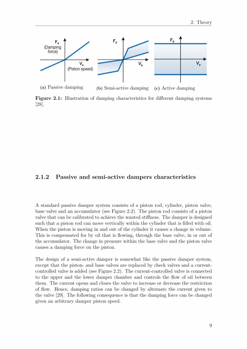
The characteristics of passive, semi-active and active dampers are illustrated in Fig-ure 2.1. In particular, the characteristics describes how the damping force variesgiven the damper piston speed. In the figure it can be seen that the potential (themarked area) of semi-active and active damping is much larger than for the passivedamper. As mentioned earlier, active suspension includes independent actuators.Hence they can deliver a bounded arbitrary force independent of the damper pistonspeed. As a consequence, active suspension has controllability potential in all fourquadrants. Semi-active suspension is more limited and only has controllability in thefirst and the third quadrant. This makes active suspension more viable to effectivelyremove vibrations, but due to some drawbacks with active suspension systems, forexample very large equipment sizes, semi-active suspension is used more often [28].

8

2. Theory

(a) Passive damping (b) Semi-active damping (c) Active damping

Figure 2.1: Illustration of damping characteristics for different damping systems[28].

2.1.2 Passive and semi-active dampers characteristics

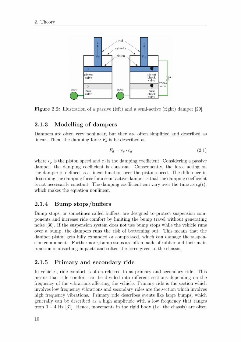
A standard passive damper system consists of a piston rod, cylinder, piston valve,base valve and an accumulator (see Figure 2.2). The piston rod consists of a pistonvalve that can be calibrated to achieve the wanted stiffness. The damper is designedsuch that a piston rod can move vertically within the cylinder that is filled with oil.When the piston is moving in and out of the cylinder it causes a change in volume.This is compensated for by oil that is flowing, through the base valve, in or out ofthe accumulator. The change in pressure within the base valve and the piston valvecauses a damping force on the piston.

The design of a semi-active damper is somewhat like the passive damper system,except that the piston- and base valves are replaced by check valves and a current-controlled valve is added (see Figure 2.2). The current-controlled valve is connectedto the upper and the lower damper chamber and controls the flow of oil betweenthem. The current opens and closes the valve to increase or decrease the restrictionof flow. Hence, damping ratios can be changed by alternate the current given tothe valve [29]. The following consequence is that the damping force can be changedgiven an arbitrary damper piston speed.

9

2. Theory

Figure 2.2: Illustration of a passive (left) and a semi-active (right) damper [29].

2.1.3 Modelling of dampersDampers are often very nonlinear, but they are often simplified and described aslinear. Then, the damping force Fd is be described as

Fd = vp · cd (2.1)

where vp is the piston speed and cd is the damping coefficient. Considering a passivedamper, the damping coefficient is constant. Consequently, the force acting onthe damper is defined as a linear function over the piston speed. The difference indescribing the damping force for a semi-active damper is that the damping coefficientis not necessarily constant. The damping coefficient can vary over the time as cd(t),which makes the equation nonlinear.

2.1.4 Bump stops/buffersBump stops, or sometimes called buffers, are designed to protect suspension com-ponents and increase ride comfort by limiting the bump travel without generatingnoise [30]. If the suspension system does not use bump stops while the vehicle runsover a bump, the dampers runs the risk of bottoming out. This means that thedamper piston gets fully expanded or compressed, which can damage the suspen-sion components. Furthermore, bump stops are often made of rubber and their mainfunction is absorbing impacts and soften the force given to the chassis.

2.1.5 Primary and secondary rideIn vehicles, ride comfort is often referred to as primary and secondary ride. Thismeans that ride comfort can be divided into different sections depending on thefrequency of the vibrations affecting the vehicle. Primary ride is the section whichinvolves low frequency vibrations and secondary rides are the section which involveshigh frequency vibrations. Primary ride describes events like large bumps, whichgenerally can be described as a high amplitude with a low frequency that rangesfrom 0− 4 Hz [31]. Hence, movements in the rigid body (i.e. the chassis) are often

10

2. Theory

associated with primary ride. Furthermore, vibrations exposed to the driver witha frequency above 4 Hz are often associated with secondary ride. These vibrationscan be associated with low amplitude and high frequency. They are often occur-ring because of imperfections in the road surface, for example very small bumps orcracks in the asphalt. Hence, secondary ride is often what passengers defines as ridecomfort. In general, issues with primary ride will occur by a vehicle at high speed,whilst issues with secondary ride will occur by a vehicle at low speed. Moreover, pri-mary ride is mostly controlled by anti-roll bars, shock absorbers and springs, whilstsecondary ride mostly depend on tire properties, suspension and bush isolation [32].

2.1.6 Quarter-car modelA quarter-car model is a two degrees of freedom (vertical displacements) model andis shown in figure 2.3. It consists of a sprung mass ms (a quarter of a car’s mass), anunsprung mass mu (mass of the wheel), two springs, and a damper [33], [34]. Thesprung mass is illustrating a quarter of the car’s chassis and weight. The sprungmass position is here called zs. The unsprung mass is the mass of the wheel and it’sposition is called zu. At the bottom of the figure a road surface is drawn and zr is theheight of the road surface’s bumps. Between the wheel mass and the road surface, aspring ku is placed, which purpose is to illustrate the characteristics and dynamicsof the tire. Between the sprung and unsprung mass a damper c and a spring ks isplaced. These are supposed to reduce the vibrations from the road surface, whichalso may improve the comfort for the passengers of the car.

Figure 2.3: Illustration of the dynamics of a quarter-car model.

In order to model the quarter-car model, Newton’s second law is used in order toderive the following equations.

11

2. Theory

ms · zs = −ks(zs − zu)− c(zs − zu) (2.2)mu · zu = ks(zs − zu) + c(zs − zu)− ku(zu − zr) (2.3)

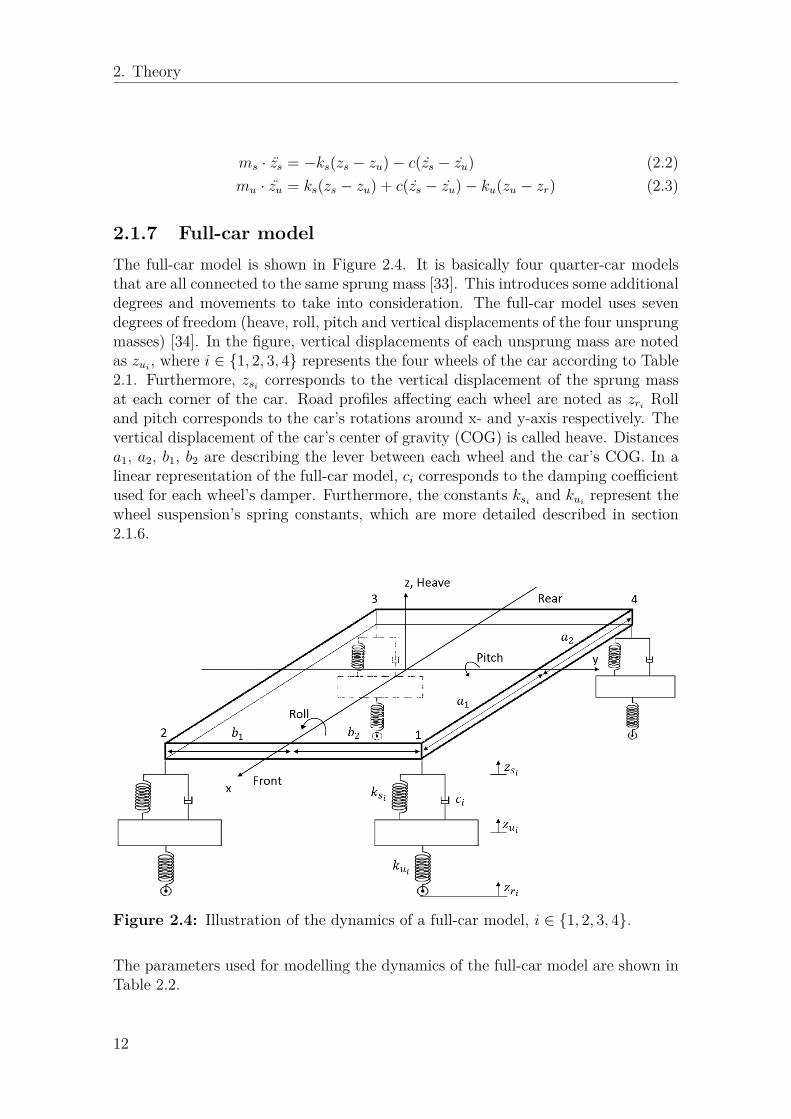
2.1.7 Full-car modelThe full-car model is shown in Figure 2.4. It is basically four quarter-car modelsthat are all connected to the same sprung mass [33]. This introduces some additionaldegrees and movements to take into consideration. The full-car model uses sevendegrees of freedom (heave, roll, pitch and vertical displacements of the four unsprungmasses) [34]. In the figure, vertical displacements of each unsprung mass are notedas zui , where i ∈ {1, 2, 3, 4} represents the four wheels of the car according to Table2.1. Furthermore, zsi corresponds to the vertical displacement of the sprung massat each corner of the car. Road profiles affecting each wheel are noted as zri Rolland pitch corresponds to the car’s rotations around x- and y-axis respectively. Thevertical displacement of the car’s center of gravity (COG) is called heave. Distancesa1, a2, b1, b2 are describing the lever between each wheel and the car’s COG. In alinear representation of the full-car model, ci corresponds to the damping coefficientused for each wheel’s damper. Furthermore, the constants ksi and kui represent thewheel suspension’s spring constants, which are more detailed described in section2.1.6.

Figure 2.4: Illustration of the dynamics of a full-car model, i ∈ {1, 2, 3, 4}.

The parameters used for modelling the dynamics of the full-car model are shown inTable 2.2.

12

2. Theory

Table 2.1: Description of how to relate i ∈ {1, 2, 3, 4} to the correct wheel.

i Wheel1 Front, Left2 Front, Right3 Rear, Right4 Rear, Left

Table 2.2: Parameters for full-car model, i ∈ {1, 2, 3, 4}.

Parameter Description Unitϕ Roll radθ Pitch radzs Heave mzsi Vertical displacement of sprung mass at each corner mzui Vertical displacement of unsprung mass at each corner mIx Roll inertia kgm2

Iy Pitch inertia kgm2

ms Sprung mass kgmui Unsprung mass kgzri Vertical displacement of road mksi Spring constant, sprung mass N/mkui Spring constant, sprung tire N/mb1 COG-distance right mb2 COG-distance left ma1 COG-distance front ma2 COG-distance rear mci Damping coefficient Ns/m

By using Newton’s second law, the linearized dynamics of the seven degree of free-dom (DOF) full-car model can be described as in the following equations of motion[35]. Worth mentioning is that the model is using small angle approximation, i.e.sin(θ) ≈ θ and cos(θ) ≈ 1, which is a good approximation, since the angles of thecar is relatively small in normal conditions of the road.

mszs = − c1

(zs − zu1 + b1ϕ− a1θ

)− c2

(zs − zu2 − b2ϕ− a1θ

)− c3

(zs − zu3 − b1ϕ+ a2θ

)− c4

(zs − zu4 + b2ϕ+ a2θ

)− ks1


)− ks2


)− ks3


)− ks4


)(2.4)

13

2. Theory

Ixϕ = − b1c1


)+ b2c2


)+ b1c3


)− b2c4


)− b1ks1


)+ b2ks2


)+ b1ks3


)− b2ks4


)(2.5)

Iyθ = a1c1


)+ a1c2


)− a2c3


)− a2c4


)+ a1ks1


)+ a1ks2


)− a2ks3


)− a2ks4


)(2.6)

mu1 zu1 = c1


)+ ks1


)− ku1

(zu1 − zr1

) (2.7)

mu2 zu2 = c2


)+ ks2


)− ku2

(zu2 − zr2

) (2.8)

mu3 zu3 = c3


)+ ks3


)− ku3

(zu3 − zr3

) (2.9)

mu4 zu4 = c4


)+ ks4


)− ku4

(zu4 − zr4

) (2.10)

2.2 Reinforcement learningReinforcement learning is an area with machine learning. Reinforcement learning isa technique that uses the fundamental ideas of “learning by doing”, and “trial anderror”. A common way of describing the learning process is the events of an agentacting in an influenceable environment. In the beginning, the agent has no informa-tion about which is the best action to take in each environment state. However, bytaking an action in the environment, the agent will get a reward in return, tellingthe agent whether the action was good or not. When taking an action, the state ofthe environment will also be updated, and the new state is given to the agent. Theloop is now closed and the agent is ready to take a new action. By repeating theprocess over and over again, the agent will learn how to act from its experience.

14

2. Theory

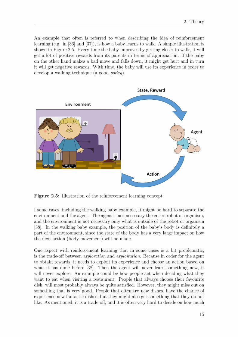
An example that often is referred to when describing the idea of reinforcementlearning (e.g. in [36] and [37]), is how a baby learns to walk. A simple illustration isshown in Figure 2.5. Every time the baby improves by getting closer to walk, it willget a lot of positive rewards from its parents in terms of appreciation. If the babyon the other hand makes a bad move and falls down, it might get hurt and in turnit will get negative rewards. With time, the baby will use its experience in order todevelop a walking technique (a good policy).

Figure 2.5: Illustration of the reinforcement learning concept.

I some cases, including the walking baby example, it might be hard to separate theenvironment and the agent. The agent is not necessary the entire robot or organism,and the environment is not necessary only what is outside of the robot or organism[38]. In the walking baby example, the position of the baby’s body is definitely apart of the environment, since the state of the body has a very large impact on howthe next action (body movement) will be made.

One aspect with reinforcement learning that in some cases is a bit problematic,is the trade-off between exploration and exploitation. Because in order for the agentto obtain rewards, it needs to exploit its experience and choose an action based onwhat it has done before [38]. Then the agent will never learn something new, itwill never explore. An example could be how people act when deciding what theywant to eat when visiting a restaurant. People that always choose their favouritedish, will most probably always be quite satisfied. However, they might miss out onsomething that is very good. People that often try new dishes, have the chance ofexperience new fantastic dishes, but they might also get something that they do notlike. As mentioned, it is a trade-off, and it is often very hard to decide on how much

15

2. Theory

one wants to explore and exploit in order to achieve the best result in the end.

2.2.1 Elements of reinforcement learningIn reinforcement learning, one usually identify the agent and the environment as thetwo main elements. These have been introduced sufficiently in the previous section.Furthermore, there are three or four sub-elements that are necessary in reinforce-ment learning; a reward, a policy, a value function and in some cases a model [38].

Policy - A policy is what decides on which action to take in each state. Thepolicy is what one wants learn or improve during learning. A policy can be verysimple, such as a very simple function or as a look-up- table that matches stateswith actions. It can also be complex, e.g. using deep neural networks. The policycan be stochastic or deterministic. Deterministic policies are used in deterministicenvironments, i.e. environments where you are given state, a particular action af-fects the environment in a specific way. Deterministic policies maps a specific stateto a specific action. Stochastic policies on the other hand, includes an uncertainty.In a specific state the chosen action may vary. Similarly, stochastic policies are usedin stochastic environments. In stochastic environments, taking a particular actionin a specific state may have several different outcomes.

Reward - A reward is a feedback signal directed to the agent, which tells howgood or bad the current action was. The reward is necessary for learning and thedesign of it can be very important in order to achieve a desired result.

Value function - A value function is a function that expresses how good it isto be in a particular state. The value function is basically a computation or esti-mation of the cumulative rewards that an agent can expect to achieve in the future,given the current state. While the reward is telling what is good to do right now,the value tells what is good in the long run.

Model - In some cases, a model of the environment can be used in order for theagent to predict consequences, i.e. the new state and reward, of taking a certainaction. Methods using models are called model-based whereas other methods arecalled model-free. Model-based methods are able to make use of planning, i.e. theycan decide on which action is the best, based on predictions of the future. Hence,model-based methods can often learn a good policy requiring fewer samples of train-ing than a model-free approach [39]. However it can be very hard to come up witha model that represents the environment good enough to make useful predictions,and there is always a risk of limiting the learning when using a model.

2.2.2 Markov decision processAMarkov decision process (MDP) is a discrete stochastic model, describing a controlprocess. It includes a set of states S, a set of actions A, a real valued reward functionr(s, a) and a state-transition probability function p(s′|s, a). The state-transition

16

2. Theory

probability function describes the probability of ending up in state s′ given states and action a. Hence, the state-transition function describes the dynamics of themodel, given the current action and state. It is necessary that the state s includesall information about the past that affects the future. If it does, the state is said tohave the Markov property. Mathematically, the Markov property can be describedas

Pr[St+1 = s′ | St] = Pr[St+1 = s′ | S0, S1, ..., St] (2.11)

where St is the state at time instance t = 1, 2, 3, ....

The relationship between reinforcement learning and the MDP can be describedas if the MDP is the framework of classic reinforcement learning [40], or to recon-nect to previous sections; the MDP is used to describe the environment and theinteraction properties with the agent. Given an agent that decides on which actionsto take, the MDP will cause a trajectory with the look of

S0, A0, R1, S1, A1, R2, S2, A2, R3, ... (2.12)

where At and Rt are the state, action and reward at time instance t = 1, 2, 3, ....

2.2.3 Rewards and returns

The reward signal is the feedback to the agent that tells whether the performedaction was good or bad. The choice of reward signal can be hard to decide andmay have a large impact on the result of the learning. It is very important that thereward signal represents the actual goal of the task, and not any subgoals. A usedexample considers the game of chess, the correct reward is to give +1 for winning and−1 for losing, not giving rewards for subgoals as taking out the opponent’s piecesand similar [38]. The goal in reinforcement learning is to maximize the cumulativereward over time. In most cases, this can also be expressed as maximizing theexpected return, where the return, Gt, is a function of the future rewards. In themost basic case with a finite episode length t ∈ [0, T ] (e.g. when playing a game),it is just the cumulative sum of the future rewards

Gt = Rt+1 +Rt+2 + ..+RT (2.13)

However, in many cases and especially control tasks, the tasks are continuous ratherthan having a finite episode length. Thus, the final time step would be T = ∞,which likely leads to an infinite return. To solve this problem, a discount factor,γ ∈ [0, 1], is often used. The discount factor decides the importance of futurerewards. The discounted return is written as

Gt = Rt+1 + γRt+2 + γ2Rt+3 + ... =∞∑i=0

γiRt+i+1 (2.14)

and by choosing γ < 1, the return becomes finite.

17

2. Theory

2.2.4 Value functions and policiesAlmost every reinforcement learning method makes use of value functions. Valuefunctions express the value of being in a particular state. The value of being in aparticular state is a computation or estimation of the expected rewards in the future,the expected return. The value function can be seen as complement to the reward,since the value function can not be calculated or estimated without rewards, andits only purpose is to achieve more rewards [38]. Furthermore, the value function ishighly dependent on the policy. The policy represents the behaviour of the agent,i.e. it decides on which actions to take. Future rewards depend on what actionsthat are performed, i.e. which policy that is used, thereby the dependency of thevalue function. For an MDP, given a policy π which is mapping states s ∈ S tocertain actions a ∈ A through the probability function π(a|s), the dependent valuefunction is defined as

vπ(s) = Eπ[Gt | St = s] = Eπ

∞∑i=0

γiRt+i+1 | St = s

=∑a

π(a|s)∑s′,r

p(s′, r|s, a)[r + γvπ(s′)

] (2.15)

In many reinforcement learning methods a similar function called the action-valuefunction is used. The action-value function returns the expected returns just as thevalue function, but it also takes a chosen action into consideration. The action-valuefunction is defined as

qπ(s, a) = Eπ[Gt | St = s, At = a] = Eπ

∞∑i=0

γiRt+i+1 | St = s, At = a

(2.16)

Value functions can be computed or estimated from experience. If an agent follows apolicy π and stores an estimate of the actual return for each state, the stored estimatewill converge to the actual return as the number of visitations of the current stateapproaches infinity. The same goes for the action-value function, with the differenceof that an estimate of each state-action pair need to be stored. However in manycases, the number of states (or state-action pairs) is too large to allow storage ofseparate values for each state. If so, a value function approximation can be used as

vπ(s,w) ≈ vπ(s) (2.17)

where w is vector of parameters. There are several different methods for functionapproximation, for instance linear combinations of features and neural networks.

2.2.5 Basic algorithms for solving MDPsIn this section, the two basic RL algorithms value iteration and policy iteration arepresented. In the following section, the algorithm Q-learning is introduced. Givena finite MDP, the three algorithms converge to an optimal policy π∗.

18

2. Theory

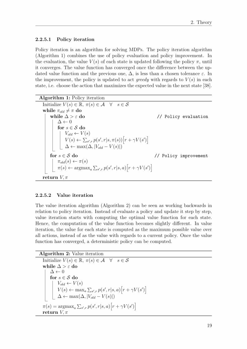
2.2.5.1 Policy iteration

Policy iteration is an algorithm for solving MDPs. The policy iteration algorithm(Algorithm 1) combines the use of policy evaluation and policy improvement. Inthe evaluation, the value V (s) of each state is updated following the policy π, untilit converges. The value function has converged once the difference between the up-dated value function and the previous one, ∆, is less than a chosen tolerance ε. Inthe improvement, the policy is updated to act greedy with regards to V (s) in eachstate, i.e. choose the action that maximizes the expected value in the next state [38].

Algorithm 1: Policy iterationInitialize V (s) ∈ R, π(s) ∈ A ∀ s ∈ Swhile πold 6= π do

while ∆ > ε do // Policy evaluation∆← 0for s ∈ S do

Vold ← V (s)V (s)← ∑

s′,r p(s′, r|s, π(s))[r + γV (s′)

]∆← max(∆, |Vold − V (s)|)

for s ∈ S do // Policy improvementπold(s)← π(s)π(s)← argmaxa

∑s′,r p(s′, r|s, a)

[r + γV (s′)

]return V, π

2.2.5.2 Value iteration

The value iteration algorithm (Algorithm 2) can be seen as working backwards inrelation to policy iteration. Instead of evaluate a policy and update it step by step,value iteration starts with computing the optimal value function for each state.Hence, the computation of the value function becomes slightly different. In valueiteration, the value for each state is computed as the maximum possible value overall actions, instead of as the value with regards to a current policy. Once the valuefunction has converged, a deterministic policy can be computed.

Algorithm 2: Value iterationInitialize V (s) ∈ R, π(s) ∈ A ∀ s ∈ Swhile ∆ > ε do

∆← 0for s ∈ S do

Vold ← V (s)V (s)← maxa

∑s′,r p(s′, r|s, a)

[r + γV (s′)

]∆← max(∆, |Vold − V (s)|)

π(s) = argmaxa∑s′,r p(s′, r|s, a)

[r + γV (s′)

]return V, π

19

2. Theory

2.2.6 Value-based, policy-based and actor-critic methodsReinforcement algorithms can often be categorized as either value-based or policy-based. In value-based methods, the policy is computed based on learned value- oraction-value functions. Policy-based methods does not learn a value function foreach state. Instead, a policy is learned directly, and it is updated continuouslyduring training. Value functions can still be used in order to update the policy, butthey are not used to select any actions. The difference can also be demonstratedby comparing value iteration (value-based) and policy iteration (policy-based) whichare presented in section 2.2.5. While policy iteration starts with a policy and updatesit continuously until convergence, value iteration does not compute any policy untilthe value functions have converged. Generally, value-based methods are able toperform very good, given a discrete action space that is small enough. Policy-basedmethods can be beneficial in cases with continuous or stochastic action spaces, butthey often end up in local optimums due to their difficulty of evaluate the currentpolicy. Aside from pure value-based and policy-based methods, there are hybridmethods called actor-critic methods. Actor-critic methods include a policy-basedactor that controls the behaviour of the agent, and a value-based critic that evaluatesthe behaviour of the agent.

2.2.7 Q-learningQ-learning is an value-based algorithm that was introduced in 1989 and makes use ofaction-value functions, Q(s, a) [41]. The algorithm basically returns a lookup table,Q-table, of the action-value for each state-action pair. It is an iterative process,where the Q-table is updated by exploring the environment. The environment isexplored for multiple episodes (e.g. game sessions or trials), and for each episode,the approximation of the action-values is updated. The algorithm makes use of theBellman equation, which expresses the action value function recursively

Q(si, a) = E[ri + γmaxa′

Q(si+1, a′)] (2.18)

The Bellman equation basically states that the value of the current state is equalto the reward of moving to the next state, added with the value of the next statetaking the best action.

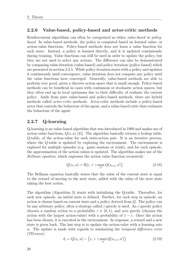
The algorithm (Algorithm 3) starts with initializing the Q-table. Thereafter, foreach new episode, an initial state is defined. Further, for each step in episode, anaction is chosen based on current state and a policy derived from Q. The policy canbe any arbitrary policy, often a strategy called ε-greedy is used. An ε-greedy policychooses a random action to a probability ε ∈ [0, 1), and acts greedy (chooses theaction with the largest action-value) with a probability of 1 − ε. Once the actionhas been chosen, it is executed in the environment. In response, a reward and a newstate is given back. The last step is to update the action-value with a learning rateα. The update is made with regards to minimizing the temporal difference error(TD-error)

δi = Q(si, a)−(ri + γmax

a′Q(si+1, a

′))

(2.19)

20

2. Theory

The TD-error is identical to the difference of the two sides in the Bellman equation,without the expected value. The sum of r+ γmaxaQ(s′, a) form what is called thetarget. The target is possibly more accurate than the current estimate of the action-value, since it includes information of the latest reward r. Given a finite MDP, thetargets and the action-values will eventually become equal.

Algorithm 3: Q-learningInitialize Q(s, a) ∈ R, ∀ s ∈ S, a ∈ Afor each episode do

Initialize sfor each step do

Choose a from s, using a policy derived from QExecute action a and observe the next state s′ and reward rQ(s, a)← Q(s, a) + α

[r + γmaxa′ Q(s′, a′)−Q(s, a)

]s← s′

until s = st

2.2.8 Deep Q-learningThe theory about reinforcement learning that has been presented in this thesis hasbeen assuming finite and discrete state and action spaces. Value-based reinforce-ment learning typically works very good in these environments, since as long as thestate and action spaces are small enough, an optimal policy can be found. However,if the combination of state and action spaces is very large, the presented algorithmswill require too much memory in order to work. In 2013, DeepMind Technologiespresented an algorithm called deep Q-learning (DQL) [13]. The algorithm com-bines Q-learning with a deep neural network (called deep Q-network or DQN) forQ-function approximation. Hence, the algorithm is capable of generalizing over verylarge state spaces, as in e.g. chess, certain video games etc. A drawback is though,that by including non-linear function approximators, as neural networks, conver-gence is not longer guaranteed. The algorithm has shown great results especiallyfor certain Atari video games, achieving superhuman performance with only the rawpixels and the score as input.

Aside from Q-learning and the deep neural network, DQL includes two fundamentaltechniques in order to work, experience replay and a target network. Experience re-play stores the recent transitions (can be a very large amount) into a buffer. Then,for every step, a minibatch of transitions is randomly sampled from the buffer toupdate the network. Since the minibatch consists of independently sampled tran-sitions, rather than correlated samples, the algorithm becomes more stable. Thetarget network is a second network, a duplicate of the original one. The differenceis that only the original network is updated during every training step. The targetnetwork is then synchronized with the original network, by every so often copy theweights from the original network. Just as its name indicates, the target networkis used for generating targets. The benefit of using a network that does not updatethat often, is that with a temporarily fixed target, the learning becomes more stable.

21

2. Theory

If the original network would be used for generating targets, the targets would beconstantly shifting and the training easily becomes unstable [42].

DQL is an off-policy algorithm. Off-policy means that the algorithm trains the agentusing experience retrieved from policies other than the current one. In contrast tooff-policy, on-policy algorithms trains the agent just using experience retrieved withthe current policy. The DQL algorithm is off-policy since it uses experience replay.Hence it uses experience (stored transitions) generated from policies other than thecurrent one. Generally, on-policy algorithms are faster, but they also risk ending upwith a policy that is just locally optimal. Off-policy algorithms may be slower, butare more flexible for finding the optimal policy.

2.2.9 Policy gradientsPolicy gradients are policy-based and improve the parameterized policy πθ(a|s) =Pr[a|s] by repeating two steps. First, a score function J(θ) is used to evaluate howgood the current policy is. (A loss function L(θ) can also be used if the goal is tominimize something rather than maximize a score.) Depending on the task and theenvironment, the score function can be different. For episodic environments, thescore function can be computed as the expected return for the entire episode.

J(θ) = Eπθ [Gt] = Eπθ [Rt+1 + γRt+2 + γ2Rt+3 + ...] (2.20)

The second step is to perform gradient ascent on the policy parameters θ, in orderto maximize the score function. The update of the parameters is then made as

θ ← θ + α∇θJ(θ) (2.21)

where α is the learning rate. Once the score function is maximized, the optimalpolicy is found.

Compared to the value-based deep Q-learning, policy gradient methods generallyconverges smoother. In Q-learning, a relatively small change of the value functionsmay result in a considerable change of the policy. This is not really the case usingpolicy gradients because of that the policy is updated stepwise. However, quite of-ten policy gradients end up in local optimum instead of global. Furthermore, policygradients have the ability to handle continuous or high dimensional action spaces,and the ability to learn stochastic policies[43].

2.2.10 Deep deterministic policy gradientWhile DQL is a solution to problems with large state spaces, it can only handlerelatively small and discrete action spaces. DQL can not be applied to continuousaction spaces since it computes the optimal action in the sense of maximizing theaction-value function. With a continuous action space, the number of actions areinfinite, and hence, some kind of iterative optimization needs to be done. In 2016,Google DeepMind presented algorithm called DDPG [12]. The algorithm uses acouple of elements that are also used in DQL (e.g. deep neural networks, target

22

2. Theory

networks and experience replay), together with policy gradients to work with con-tinuous action spaces.

The algorithm is based on the actor-critic off-policy deterministic policy gradient(DPG) algorithm that was introduced in 2014 [44]. The algorithm aims to learna deterministic policy that maximizes the score function, i.e. the expected returnin equation (2.20). The algorithm makes use of a parameterized critic Q(s, a|θQ)defining the action value of state-action pairs, and a parameterized deterministicactor function µ(s|θµ) which maps states to specific actions. Thus, the actor func-tion specifies the current policy. The critic is updated as in Q-learning, using theBellman equation. The actor is updated by following the gradient of the policy’sperformance, i.e. the gradient of the expected return

∇θµJ ≈ E[∇θµQ(s, a|θQ)|s=st,a=µ(st|θµ)]= E[∇aQ(s, a|θQ)|s=st,a=µ(st)∇θµµ(s|θµ)|s=st ]

(2.22)

The target network approach in the DDPG is similar to what is used in DQL. Themethod has been adapted to the actor-critic architecture with two networks. Fur-ther, the main difference is the “soft” update of the target networks. The weightsof the target networks are updated with a particular update rate for every step, τ ,rather than just copy the weights from the original network every so often. Hence,the target networks will slowly track the original networks, improving stability ofthe learning.

As previously mentioned, reinforcement learning often needs to deal with the trade-off between exploration and exploitation. However, since the DDPG is off-policy,it can deal with the problem of exploration independently from learning. Whilelearning with the DDPG, the exploration is made by adding noise to the actionsgenerated from the actor policy.

µ′(st) = µ(st|θµt ) +N (2.23)

Here, µ(st|θµt ) is the actor policy, N is the noise and µ′(st) is the exploration policy.In the original paper, Ornstein-Uhlenbeck noise is used. The correlated noise processsatisfies the stochastic differential equation

dxt = θ(µ− xt)dt+ σdWt (2.24)

where µ is a drift constant, θ and σ are positive parameters and Wt is the Wienerprocess [45]. However, the action noise can be chosen arbitrary to fit the environ-ment [12].

The DDPG is presented in its completeness as Algorithm 4. It is noticeable that alloperations are made within the inner loop. Thus, the algorithm is able to operatein both episodic and fully continuous environments.

23

2. Theory

Algorithm 4: Deep deterministic policy gradientInitialize critic network Q(s, a|θQ) and actor network µ(s|θµ) with weights θQand θµInitialize target networks Q′ and µ′ with target weights θQ′ ← θQ andθµ′ ← θµ

Initialize replay buffer Rfor each episode do

Receive initial observation state s1Initialize exploration noise process Nfor each step t ∈ [1, T ] do

Choose at = µ(st|θµt ) +Nt, using the current policy and explorationnoiseExecute action at and observe the new state st+1 and reward rtStore the transition (st, at, rt, st+1) in RSample random minibatch of N transitions (si, ai, ri, si+1) from RSet the targets yi = ri + γQ′

(si+1, µ

′(si+1|θµ′)|θQ′

)Update the critic by minimizing the loss L = 1

N

∑i

(yi −Q(si, ai|θQ)

)2

Update the policy of the actor using the sampled policy gradient

∇θµJ ≈ ∇aQ(s, a|θQ)|s=si,a=µ(si)∇θµµ(s|θµ)|s=si

Update the target networks

θQ′ ← τθQ + (1− τ)θQ′

θµ′ ← τθµ + (1− τ)θµ′

2.3 Artificial neural networks

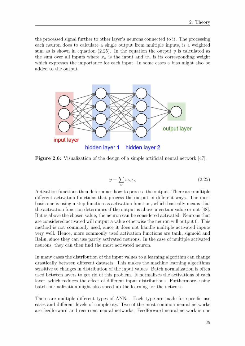
In many reinforcement learning methods, especially those made for larger statespaces, artificial neural networks (ANNs) are used. They are computing systemsinspired by the biological neural networks that exists in, for instance, human brains.ANNs can be described as massive parallel computing systems that consists of ex-tremely many simple processors with a large number of interconnections [46]. Thus,ANNs are a good tool for finding patterns in very complex systems. These patternscan often be way too complex for humans to find, and even harder to explicitly teachmachines to recognize [47].

ANNs often consists of multiple layers, which are divided into input layers, hid-den layers and output layers. These layers can be seen in Figure 2.6, where eachlayer consists of artificial neurons (the white circles), which often also are callednodes or units. Each neuron receives inputs (visualized as the arrows in the figure)from a specified number of neurons from other layers, or from an external source, andoutput a single signal. When a neuron receives a signal, it can process it and send

24

2. Theory

the processed signal further to other layer’s neurons connected to it. The processingeach neuron does to calculate a single output from multiple inputs, is a weightedsum as is shown in equation (2.25). In the equation the output y is calculated asthe sum over all inputs where xn is the input and wn is its corresponding weightwhich expresses the importance for each input. In some cases a bias might also beadded to the output.

Figure 2.6: Visualization of the design of a simple artificial neural network [47].

y =∑n

wnxn (2.25)

Activation functions then determines how to process the output. There are multipledifferent activation functions that process the output in different ways. The mostbasic one is using a step function as activation function, which basically means thatthe activation function determines if the output is above a certain value or not [48].If it is above the chosen value, the neuron can be considered activated. Neurons thatare considered activated will output a value otherwise the neuron will output 0. Thismethod is not commonly used, since it does not handle multiple activated inputsvery well. Hence, more commonly used activation functions are tanh, sigmoid andReLu, since they can use partly activated neurons. In the case of multiple activatedneurons, they can then find the most activated neuron.

In many cases the distribution of the input values to a learning algorithm can changedrastically between different datasets. This makes the machine learning algorithmssensitive to changes in distribution of the input values. Batch normalization is oftenused between layers to get rid of this problem. It normalizes the activations of eachlayer, which reduces the effect of different input distributions. Furthermore, usingbatch normalization might also speed up the learning for the network.

There are multiple different types of ANNs. Each type are made for specific usecases and different levels of complexity. Two of the most common neural networksare feedforward and recurrent neural networks. Feedforward neural network is one

25

2. Theory

of the most basic types of networks. It uses a technique that only can send infor-mation in one direction between input and output. A recurrent neural network cansend information in multiple directions, which makes the technique suitable for morecomplex tasks as it possesses greater learning abilities.

26

3Methods

In this chapter, the process and the used methods are presented. In the first twosections, the modelling of a quarter-car and a full-car are described. In the sectionthat follows, the control approach using reinforcement learning is presented.

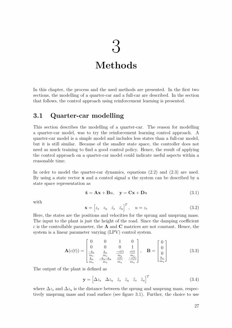
3.1 Quarter-car modellingThis section describes the modelling of a quarter-car. The reason for modellinga quarter-car model, was to try the reinforcement learning control approach. Aquarter-car model is a simple model and includes less states than a full-car model,but it is still similar. Because of the smaller state space, the controller does notneed as much training to find a good control policy. Hence, the result of applyingthe control approach on a quarter-car model could indicate useful aspects within areasonable time.

In order to model the quarter-car dynamics, equations (2.2) and (2.3) are used.By using a state vector x and a control signal u the system can be described by astate space representation as

x = Ax + Bu, y = Cx + Du (3.1)

withx =

[zs zu zs zu

]T, u = zr (3.2)

Here, the states are the positions and velocities for the sprung and unsprung mass.The input to the plant is just the height of the road. Since the damping coefficientc is the controllable parameter, the A and C matrices are not constant. Hence, thesystem is a linear parameter varying (LPV) control system.

A(c(t)) =

0 0 1 00 0 0 1−ksms

ksms

−c(t)ms

c(t)ms

ksmu

−ks−kumu

c(t)mu

−c(t)mu

, B =

000kumu

(3.3)

The output of the plant is defined as

y =[∆zs ∆zu zs zu zs zu

]T(3.4)

where ∆zs and ∆zu is the distance between the sprung and unsprung mass, respec-tively unsprung mass and road surface (see figure 3.1). Further, the choice to use

27

3. Methods

∆zs and ∆zu, instead of the total height, was mainly based on the reality aspects,where ∆zs actually can be measured while zs can not. Consequently, the matricesC and D are then defined as

Figure 3.1: Illustration of the dynamics of a quarter-car model.

C =

1 −1 0 00 1 0 00 0 1 00 0 0 1−ksms

ksms

−cms

cms

ksmu

−ks−kumu

cmu

−cmu

, D =

0−1000kumu

(3.5)

The system is continuous and in order to design a controller, the system needs tobe discretized. The discretized system is then defined as

xk+1 = Axk + Buk, yk = Cxk + Duk (3.6)

whereA = I −∆tA, B = ∆tB (3.7)

∆t is here defined as the period time, and I is the identity matrix.

To be able to understand the performance of the trained controller, controllinga semi-active damper, it was compared to a passive damper running over the exactsame road profile. The passive damper was easily designed such that, instead ofusing a controller to choose different damping coefficients, the damper coefficientwas set to a constant. Hence, the performance for the trained controller, relative tothe passive damper, could be achieved.

28

3. Methods

3.2 Full-car modelling

This section describes the full-car model that was created and used for training andevaluation. The model is based on the linearized dynamics from section 2.1.7 withsome added nonlinearities.

3.2.1 DynamicsTo model the full-car dynamics, equations (2.4)-(2.10) were used with some modifi-cations. To get a more precise model, nonlinear dampers were used instead of linearrepresentations. Also, nonlinear bump stops / buffers were added to the model (im-plying forces when the dampers reach their compression or expansion limit). Withthe modifications, the nonlinear dynamics are described as

mszs =4∑i=1

(Fdi(cdi , vdi) + Fbi(pdi)

)− ks1


)− ks2


)− ks3


)− ks4


) (3.8)

Ixϕ = b1

(Fd1(cd1 , vd1) + Fb1(pd1)

)− b2

(Fd2(cd2 , vd2) + Fb2(pd2)

)− b1

(Fd3(cd3 , vd3) + Fb3(pd3)

)+ b2

(Fd4(cd4 , vd4) + Fb4(pd4)

)− b1ks1


)+ b2ks2


)+ b1ks3


)− b2ks4


)(3.9)

Iyθ = − a1

(Fd1(cd1 , vd1) + Fb1(pd1)

)− a1

(Fd2(cd2 , vd2) + Fb2(pd2)

)+ a2

(Fd3(cd3 , vd3) + Fb3(pd3)

)+ a2

(Fd4(cd4 , vd4) + Fb4(pd4)

)+ a1ks1


)+ a1ks2


)− a2ks3


)− a2ks4


)(3.10)

mu1x1 =− c1

(Fd1(cd1 , vd1) + Fb1(pd1)

)+ ks1


)− ku1

(zu1 − zr1

) (3.11)

mu2x2 =− c2

(Fd2(cd2 , vd2) + Fb2(pd2)

)+ ks2


)− ku2

(zu2 − zr2

) (3.12)

29

3. Methods

mu3x3 =− c3

(Fd3(cd3 , vd3) + Fb3(pd3)

)+ ks3


)− ku3

(zu3 − zr3

) (3.13)

mu4x4 =− c4

(Fd4(cd4 , vd4) + Fb4(pd4)

)+ ks4


)− ku4

(zu4 − zr4

) (3.14)

Most notations are defined just as in Table 2.2, with a few exceptions. Fdi(cdi , vdi)is the damping force at wheel i, depending on the control current to the damper cdiand the damper velocity vdi . A positive damper velocity corresponds to an extensionand a negative damper velocity corresponds to a compression of the damper. Thebuffer forces are denoted Fbi(pdi), and depends on the position of the damper pdi .The positions and velocities of the dampers are defined as

pd1 = zs − zu1 + b1ϕ− a1θ, vd1 = zs − zu1 + b1ϕ− a1θ

pd2 = zs − zu2 − b2ϕ− a1θ, vd2 = zs − zu2 − b2ϕ− a1θ

pd3 = zs − zu3 − b1ϕ+ a2θ, vd3 = zs − zu3 − b1ϕ+ a2θ

pd4 = zs − zu4 + b2ϕ+ a2θ, vd4 = zs − zu4 + b2ϕ+ a2θ

(3.15)

The characteristics of the buffer forces are shown in Figure 3.2. The magnitude ofthe buffer forces quickly get much larger than the maximum controllable dampingforce. Hence, to achieve a smooth behaviour of the car body, the controller shouldact such that buffer forces are avoided if possible.

Figure 3.2: Illustration of the buffer forces for the front and rear wheels, dependingon the damper piston position.

30

3. Methods

In Figure 3.3, the characteristic of a semi-active damper is shown. The area be-tween the upper and lower limits, marked with bright grey, illustrates the possibleforce outputs from the damper. The stiffness of the damper, and thereby also theforce, can be changed for an arbitrary piston speed by varying the current to thedamper. The more current, the stiffer the damper becomes. The characteristics ofthe damper is linear between the lines ’Max’ and ’Mid’ stiffness and between ’Min’and ’Mid’ stiffness. The stiffness of the damper, and the following force, is controlledby the current to the damper. Given a specific damper velocity, the current decideswhere, between the upper and the lower limit, the force output can be found.

Figure 3.3: Characteristic of semi-active damper, depending on the damper pistonvelocity and the damper control signal.

To increase the precision of the model, a response delay representing the behaviourof the dampers when the input current is changed, was included. The response de-lay was modelled as a pure time delay and a change of rate limitation for changingthe current to the damper. The pure delay is the time between sending a signal tothe damper, to when the damper characteristics actually starts changing, based onthe new signal. The change of rate limitation limits how fast the damper stiffnesscan change. This property is quite complex and nonlinear, but in this thesis it isapproximated with a linear function.

The coefficient limiting the maximum change of rate of the damper, was deter-mined using a step response of the real damper. The coefficient kcd was calculatedas

kcd = ∆F∆T (3.16)

where ∆F is the change in force, from minimum to 90% of maximum, and ∆T isthe corresponding time.

31

3. Methods

The equations achieved for updating the force according to the delay are then for-mulated as

Fnew =

Fset, if |Fnew − Fset| ≤ kcd dt

Fset + kcd dt, if Fnew − Fset > kcd dt

Fset − kcd dt, if Fnew − Fset < −kcd dt

where Fset is the setting value (the chosen force from the controller), dt is the sam-pling time between each new setting value and Fnew is the force affected by the delayand hence, the force used to update the plant.

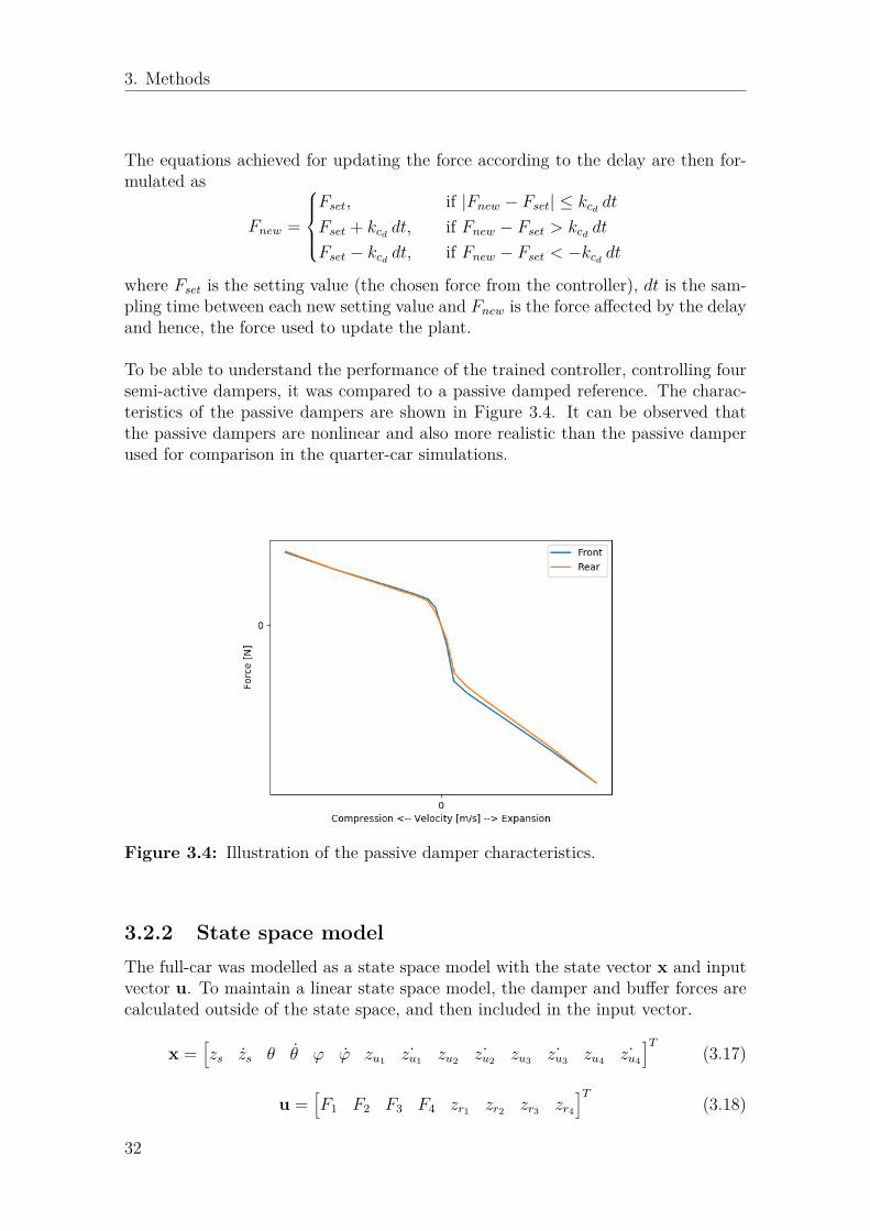
To be able to understand the performance of the trained controller, controlling foursemi-active dampers, it was compared to a passive damped reference. The charac-teristics of the passive dampers are shown in Figure 3.4. It can be observed thatthe passive dampers are nonlinear and also more realistic than the passive damperused for comparison in the quarter-car simulations.

Figure 3.4: Illustration of the passive damper characteristics.

3.2.2 State space modelThe full-car was modelled as a state space model with the state vector x and inputvector u. To maintain a linear state space model, the damper and buffer forces arecalculated outside of the state space, and then included in the input vector.

x =[zs zs θ θ ϕ ϕ zu1 ˙zu1 zu2 ˙zu2 zu3 ˙zu3 zu4 ˙zu4

]T(3.17)

u =[F1 F2 F3 F4 zr1 zr2 zr3 zr4

]T(3.18)

32

3. Methods

Here, Fi is the sum of the damping force and potential buffer force for each wheel,i.e. Fi = Fdi +Fbi for i = 1, 2, 3, 4. zri is the height of the road affecting each wheel.The output vector of the system is defined as

y =[zs zs θ θ θ ϕ ϕ ϕ ∆z1 · · · ∆z4 ∆z1 · · · ∆z4

]T(3.19)

where ∆zi is the expansion or the compression distance of the damper at wheel i,and ∆zi is the corresponding velocity.

The dynamics can be described with the approximate discrete state space model

xk+1 = (I + A∆t)xk + B∆tukyk = Cxk + Duk

(3.20)

where xk, uk and yk is the state vector, the input vector and the output vector atstep k, respectively. I is the identity matrix and ∆t is the step size. The matricesA and B are derived from the set of dynamic equations f (equation (3.8) - (3.14)),as ∂f

∂x and ∂f∂u respectively. The matrices C and D are appropriate matrices for

achieving the output specified in (3.19).

3.3 Reinforcement learning controlIn this section, the control problem is defined and a reinforcement learning approachfor controlling semi-active suspension is presented. The approach is applied to botha quarter-car environment and a full-car environment, which previously have beenpresented in section 3.1 and 3.2.

3.3.1 Control problem identificationRecalling from section 2.2, reinforcement learning algorithms learn the agent howto act from experience. The agent basically gets to try different actions in theenvironment of interest, and with time it learns how it should act. In this thesis,reinforcement learning is used to train a controller for semi-active dampers. Thus,the agent is identified as the controller. The environment is a vertical vehicle model(quarter-car or full-car) that is running over a specified road. In order to controlsemi-active suspension systems, as in the quarter-car and full-car environments, alearning algorithm for continuous action spaces is needed. Furthermore, aside fromthe observed outputs from the two models, the road profile is said to be knownfor a specific distance in front of the car. This data is referred to as road previewdata. When adding road preview data to the observation space (i.e. the data thatis observed by the agent), the state space quickly becomes very large. Hence, thealgorithm need to be able to handle large state spaces as well.

3.3.2 Deep deterministic policy gradient approachBased on the specified requirements in section 3.3.1, the DDPG (Algorithm 4) isa suitable learning algorithm. It is designed for continuous action spaces and can

33

3. Methods

handle large state spaces. Also, it is an off-policy algorithm that strives to reachthe global optimum, and does not get stuck in a local optimum. Another advantageis that the algorithm is versatile in the sense of that it is compatible with bothepisodic and fully continuous environments. This property allows for learning bothby running over one specific road for several times, and by running over a neverending road for a specific time.

The DDPG algorithm was implemented in Python using the deep learning libraryTFLearn. The implementation of the algorithm was made based on [49], and strictlyfollows the structure of Algorithm 4. Just as in the original paper [12], Ornstein-Uhlenbeck noise was used for exploration.

The training of the agent was made by simulating the vehicle model running over aroad profile, with the agent controlling the semi-active dampers. By trying out dif-ferent actions given different observation states (i.e. trying out different stiffnessesof the semi-active dampers in different situations), and get a corresponding reward,the agent is able to learn how to act given different observation states. The obser-vation state vector that is observed by the agent consists of the output vector of thevehicle model y, and the road preview vector zr, as

yobs =[

yzr

](3.21)

The road preview vector describes how the road is changing in front of the wheels.Every state in the vector describes the road height difference between the currentlongitudinal position and a future longitudinal position. The number of previewstates for each wheel is specified as N and the longitudinal distance between thestates are defined as ∆prev (the density of the preview states). These parametersare selected and heavily impact the size of the road preview vector. Furthermore,the training were made with a constant velocity of the car. Different velocities weretested for different roads, but within each training session the velocity was constant.

The reward is the feedback to the agent, and hence fundamental for learning adesired behaviour. The desired behaviour of the controller is to maximize ride com-fort and handling of the car. Two factors that in many ways are subjective. Sincethis thesis does not investigate which variables that contributes to a optimal ridecomfort and handling, the shaping of the reward signal has been very simple.

When training a neural network, a the hyper-parameters need to be specified.Hyper-parameters are parameters that affect the learning and are set before thelearning process begins. The choice of hyper-parameters were inspired by [12] andare shown in Table 3.1. A couple of different setups were investigated, but did notshow satisfactory results.

34

3. Methods

Table 3.1: Hyper-parameters for the DDPG.

Description ValueActor network learning rate 0.0001Critic network learning rate 0.001

Discount factor 0.99Update rate of target networks 0.001

Buffer size 1000000Minibatch size 64

3.3.3 Quarter-car controlThe purpose of training a neural network controller for a quarter-car environmentwas to get an indication for how the DDPG algorithm would work in a wheel suspen-sion environment. Furthermore, since a quarter-car model implies a much simplerenvironment, customization of the learning algorithm and the controller is easierand more time efficient. Customization settings and results from the quarter-carmodel could then be used in the full-car model.

A quarter-car controller was trained with the DDPG algorithm on the state spacemodel presented in section 3.1. Thus, the control signal decided by the controllerwas the bounded damping coefficient of the semi-active damper. The observationstate vector for the controller consisted of the output from the plant (3.4), and theroad preview data

yobs =[∆zs ∆zu zs zu zs zu ∆zr1 . . . ∆zrN

]T(3.22)

Here, every preview state, ∆zrj ∀ j ∈ [1, N ], represents the height difference be-tween the current height of the road and a future height of the road.

The architecture of the actor and the critic network that was used for the quarter-caris similar to what was used in [12], both including two hidden layers with rectifiedlinear unit (ReLU) functions, and batch normalization. Also, the output layer ofthe actor network is a tanh() layer. The critic network takes both observation statesand actions as input. However, the actions are not included until the second hiddenlayer. This is a design that experimentally has shown to work well [49].

The controller was trained on a short road, running over it for several times. Dif-ferent road preview setups were used, as well as different velocities of the car anddifferent setups of neural networks. The reward function, used for learning, was setto depend on the acceleration and jerk of the body, zs and

...z s respectively, as

R = −|zs| − 0.003 · |...z s| (3.23)

The small jerk term was included in the reward function to compensate for the factthat the simple model allows to change the damping coefficient to any value withinthe bounds instantly. Hence, small oscillations of the body acceleration could be

35

3. Methods

prevented. The reward is mainly focusing on reducing the body acceleration, whichis a common measurement for wheel suspension.

3.3.4 Full-car controlThe DDPG algorithm was also applied to the full-car model presented in section 3.2.Since the model includes four semi-active dampers, the controller had four actions,the damper control signals cdi , i = 1, 2, 3, 4. These signals have been describedpreviously in section 3.2.1. The states observed by the controller consist of theoutput vector from the full-car plant (3.19) and the road preview data as in (3.21).The preview vector is defined as

zr =[∆zr1,1 ∆zr1,2 · · · ∆zri,j · · · ∆zr4,N−1 ∆zr4,N

]T(3.24)

where i ∈ [1, 4] defines the wheel number and j ∈ [1, N ] defines the preview stepnumber. Similarly as to the quarter-car, zri,j represents the height difference be-tween the current height of the road for the current wheel and a future height ofthe road for the current wheel. The preview length and density was experimentallydecided. During experiments, a preview of 15 steps for each wheel, that togethercovered just over 0.2 s of the road in front of the wheels showed good results. Areasonable time considering the response time of the dampers. However, for imple-mentation simplicity, the preview was defined in distance rather than time ahead ofthe vehicle. Due to this, the preview setup in terms of preview distance and densitywas needed to be changed for different vehicle velocities.

Just as for the quarter-car, both the actor and the critic network was set to includetwo fully connected layers with ReLU activation functions, batch normalization andtanh() layers as output layers. The only difference was the size of the networks.Because of the much larger state and action space, deeper networks were used.

Full-car controllers were trained both episodically and continuously, i.e. runningover a short road for several times and running over a very long road for just onetime. Different road preview setups were used, as well as different hyper-parameters,different velocities of the car and different neural network settings. The reward wasdefined as the negative sum of the accelerations (roll, pitch and heave).

R = −|ϕ| − |θ| − |zs| (3.25)

The evaluations of the trained controllers were made both using the training en-vironment and IPG CarMaker. When evaluated in the training environment, thecontroller is compared to a passive reference. IPG CarMaker includes a more com-plex model of the full-car, as well as the opportunity to compare the trained con-trollers to a couple of other controllers. The controllers used for comparison is aContinuously Controlled Damping controller (CCD) and an improved version of thenonlinear MPC proposed by [3]. CCD is a control method for semi-active suspensionwithout preview that is used in some of today’s cars.

36

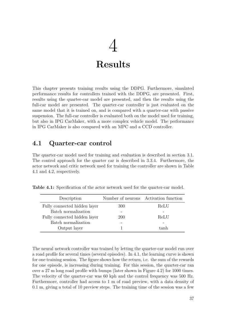
4Results

This chapter presents training results using the DDPG. Furthermore, simulatedperformance results for controllers trained with the DDPG, are presented. First,results using the quarter-car model are presented, and then the results using thefull-car model are presented. The quarter-car controller is just evaluated on thesame model that it is trained on, and is compared with a quarter-car with passivesuspension. The full-car controller is evaluated both on the model used for training,but also in IPG CarMaker, with a more complex vehicle model. The performancein IPG CarMaker is also compared with an MPC and a CCD controller.

4.1 Quarter-car control

The quarter-car model used for training and evaluation is described in section 3.1.The control approach for the quarter car is described in 3.3.4. Furthermore, theactor network and critic network used for training the controller are shown in Table4.1 and 4.2, respectively.

Table 4.1: Specification of the actor network used for the quarter-car model.

Description Number of neurons Activation functionFully connected hidden layer 300 ReLU

Batch normalization - -Fully connected hidden layer 200 ReLU

Batch normalization - -Output layer 1 tanh

The neural network controller was trained by letting the quarter-car model run overa road profile for several times (several episodes). In 4.1, the learning curve is shownfor one training session. The figure shows how the return, i.e. the sum of the rewardsfor one episode, is increasing during training. For this session, the quarter-car ranover a 27 m long road profile with bumps (later shown in Figure 4.2) for 1000 times.The velocity of the quarter-car was 60 kph and the control frequency was 500 Hz.Furthermore, controller had access to 1 m of road preview, with a data density of0.1 m, giving a total of 10 preview steps. The training time of the session was a few

37

4. Results

Table 4.2: Specification of the critic network used for the quarter-car contrller.



Batch normalization - -Output layer 1 linear

hours on a regular laptop.

Figure 4.1: Return during training of quarter-car controller.

Evaluation results of the trained controller, compared with a passive damped refer-ence, are shown in Figure 4.2. Here, the road profile is presented together with thebody acceleration and the chosen action from the controller. The road profile is thesame as the one the controller was trained on. By comparing the body accelerationsof the two systems, it is clear that the semi-active system with the trained controllerperforms significantly better than the passive system. In Table 4.3, the root meansquare (RMS) values of the reward and the body acceleration are presented for thesemi-active system with the trained controller and the passive system. Generally,the RMS is around 40% better for the trained controller. It can also be observedthat the controller has a clear policy, where it chooses low damping coefficients whenapproaching bumps, and high coefficients to damp rebounds. The passive damperuses a constant damping coefficient of 1500 Ns/m.

38

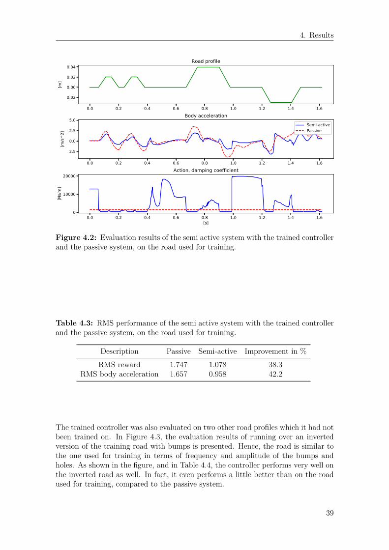
4. Results

0.0 0.2 0.4 0.6 0.8 1.0 1.2 1.4 1.6

−0.02

0.00

0.02

0.04[m

]Road rofile

0.0 0.2 0.4 0.6 0.8 1.0 1.2 1.4 1.6

−2.5

0.0

2.5

5.0

[m/s^2

]

Body accelerationSemi-activePassive

0.0 0.2 0.4 0.6 0.8 1.0 1.2 1.4 1.6[s]

0

10000

20000

[Ns/m]

Action, damping coefficient

Figure 4.2: Evaluation results of the semi active system with the trained controllerand the passive system, on the road used for training.

Table 4.3: RMS performance of the semi active system with the trained controllerand the passive system, on the road used for training.

Description Passive Semi-active Improvement in %RMS reward 1.747 1.078 38.3

RMS body acceleration 1.657 0.958 42.2

The trained controller was also evaluated on two other road profiles which it had notbeen trained on. In Figure 4.3, the evaluation results of running over an invertedversion of the training road with bumps is presented. Hence, the road is similar tothe one used for training in terms of frequency and amplitude of the bumps andholes. As shown in the figure, and in Table 4.4, the controller performs very well onthe inverted road as well. In fact, it even performs a little better than on the roadused for training, compared to the passive system.

39

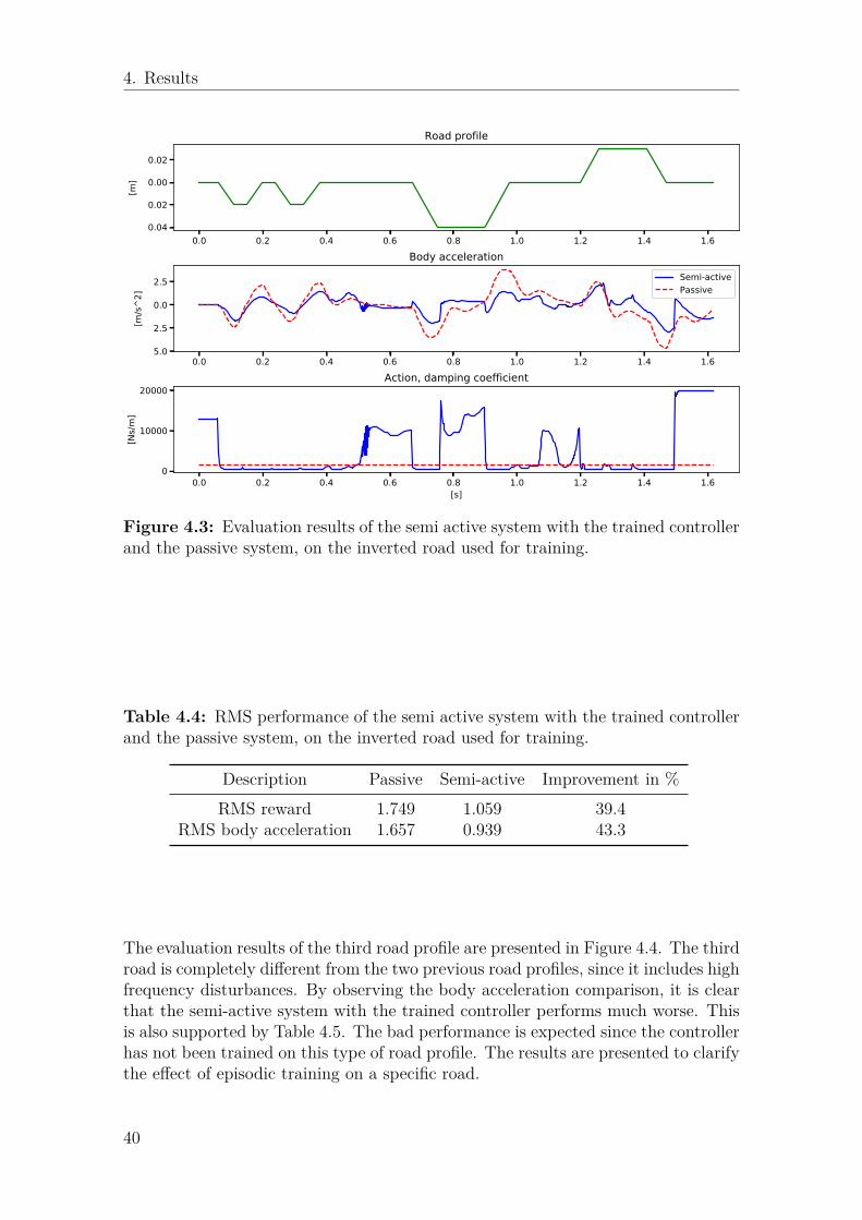
4. Results

0.0 0.2 0.4 0.6 0.8 1.0 1.2 1.4 1.6−0.04

−0.02

0.00

0.02

[m]

Road rofile

0.0 0.2 0.4 0.6 0.8 1.0 1.2 1.4 1.6−5.0

−2.5

0.0

2.5

[m/s^2

]


0.0 0.2 0.4 0.6 0.8 1.0 1.2 1.4 1.6[s]

0

10000

20000

[Ns/m]


Figure 4.3: Evaluation results of the semi active system with the trained controllerand the passive system, on the inverted road used for training.

Table 4.4: RMS performance of the semi active system with the trained controllerand the passive system, on the inverted road used for training.

Description Passive Semi-active Improvement in %RMS reward 1.749 1.059 39.4


The evaluation results of the third road profile are presented in Figure 4.4. The thirdroad is completely different from the two previous road profiles, since it includes highfrequency disturbances. By observing the body acceleration comparison, it is clearthat the semi-active system with the trained controller performs much worse. Thisis also supported by Table 4.5. The bad performance is expected since the controllerhas not been trained on this type of road profile. The results are presented to clarifythe effect of episodic training on a specific road.

40

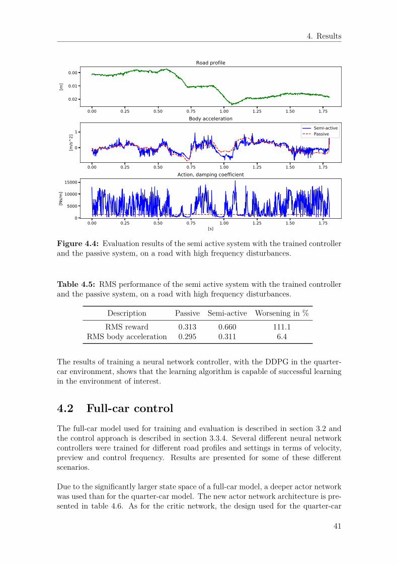
4. Results

0.00 0.25 0.50 0.75 1.00 1.25 1.50 1.75

−0.02

−0.01

0.00

[m]

Road profile

0.00 0.25 0.50 0.75 1.00 1.25 1.50 1.75

0

1

[m/ ^2

]


0.00 0.25 0.50 0.75 1.00 1.25 1.50 1.75[s]

0

5000

10000

15000

[Ns/m]


Figure 4.4: Evaluation results of the semi active system with the trained controllerand the passive system, on a road with high frequency disturbances.

Table 4.5: RMS performance of the semi active system with the trained controllerand the passive system, on a road with high frequency disturbances.

Description Passive Semi-active Worsening in %RMS reward 0.313 0.660 111.1


The results of training a neural network controller, with the DDPG in the quarter-car environment, shows that the learning algorithm is capable of successful learningin the environment of interest.

4.2 Full-car controlThe full-car model used for training and evaluation is described in section 3.2 andthe control approach is described in section 3.3.4. Several different neural networkcontrollers were trained for different road profiles and settings in terms of velocity,preview and control frequency. Results are presented for some of these differentscenarios.

Due to the significantly larger state space of a full-car model, a deeper actor networkwas used than for the quarter-car model. The new actor network architecture is pre-sented in table 4.6. As for the critic network, the design used for the quarter-car

41

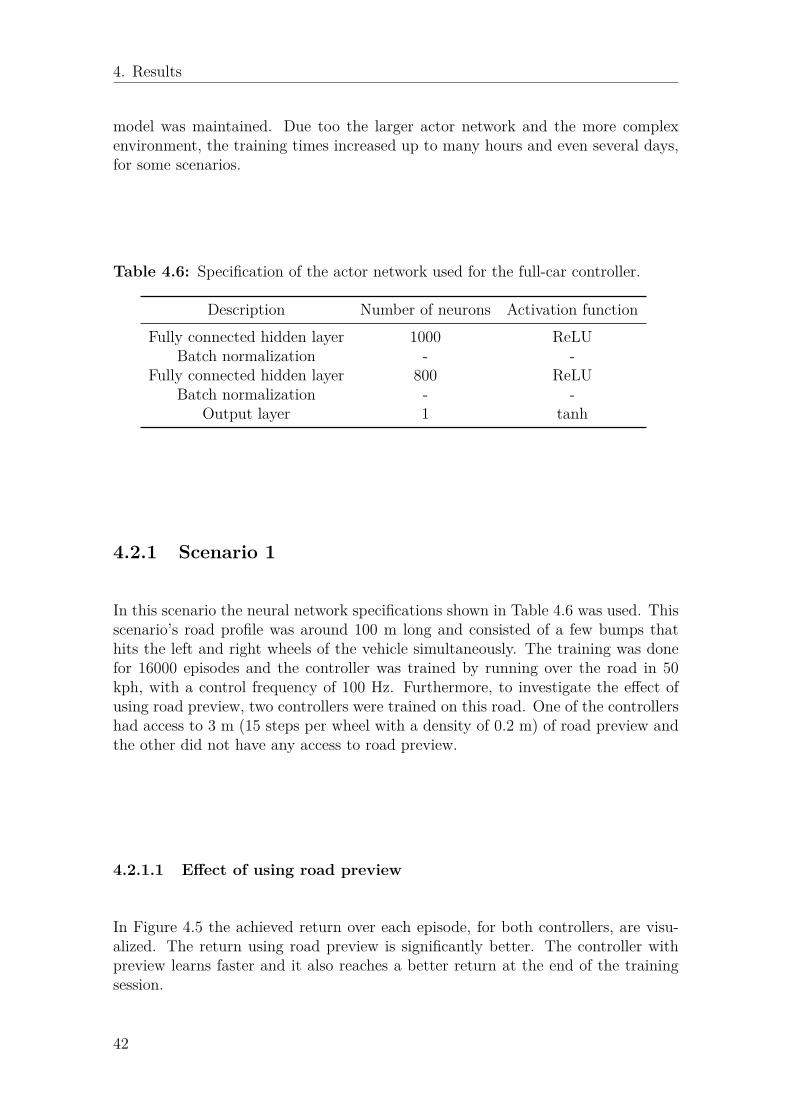
4. Results

model was maintained. Due too the larger actor network and the more complexenvironment, the training times increased up to many hours and even several days,for some scenarios.

Table 4.6: Specification of the actor network used for the full-car controller.



Batch normalization - -Output layer 1 tanh

4.2.1 Scenario 1

In this scenario the neural network specifications shown in Table 4.6 was used. Thisscenario’s road profile was around 100 m long and consisted of a few bumps thathits the left and right wheels of the vehicle simultaneously. The training was donefor 16000 episodes and the controller was trained by running over the road in 50kph, with a control frequency of 100 Hz. Furthermore, to investigate the effect ofusing road preview, two controllers were trained on this road. One of the controllershad access to 3 m (15 steps per wheel with a density of 0.2 m) of road preview andthe other did not have any access to road preview.

4.2.1.1 Effect of using road preview

In Figure 4.5 the achieved return over each episode, for both controllers, are visu-alized. The return using road preview is significantly better. The controller withpreview learns faster and it also reaches a better return at the end of the trainingsession.

42

4. Results

(a) Controller with preview (b) Controller without preview

Figure 4.5: Comparison of the return achieved during training between a controllerwith road preview and a controller without road preview.

4.2.1.2 Evaluation on training model

The trained controllers were then evaluated on the same model and road whichthey were trained on. The performance, compared to a full-car system with passivedampers, are presented in Figure 4.6 and in Table 4.7. It can be observed thatboth controllers perform better than the passive reference in terms of RMS reward,and the controller using preview performs the best. The controller with previewperforms very good in terms of heave and pitch acceleration. More specifically, theimprovement compared to the passive reference is 16% and 28%, for heave and pitchrespectively. Regarding the roll performance, the trained controller performs muchworse than the passive reference. The reason for this behavior is because the currentroad is identical for the left and right side of the car at all time, as can be seen inthe top of Figure 4.6. Furthermore, the model of the car is symmetric around theroll-axis. For these reasons, the passive reference does not induce any roll. Thetrained controller does induce a roll though. This is because the controller has beentrained by trying random actions for each wheel, and the learned policy is not en-tirely optimal. However, it should be noted that the roll acceleration is rather smallcompared to the heave and pitch accelerations.

Table 4.7: RMS performance comparison between a passive reference, a trainedcontroller without road preview and a trained controller with road preview.

Description Passive No preview 3m previewRMS heave acceleration 1.11 1.17 0.94RMS pitch acceleration 1.39 1.04 1.00RMS roll acceleration 0.00 0.22 0.19

RMS reward 2.30 2.18 1.90

43

4. Results

2.5 3 3.5 4 4.5 5-0.05

0

0.05

[m]

Road profile

FL

FR

RR

RL

2.5 3 3.5 4 4.5 50

1

2

[A]

Control signal NN-control 3m preview

FL

FR

RR

RL

2.5 3 3.5 4 4.5 5-5

0

5

[m/s

2]

Heave acceleration

Passive

No preview

3m preview

2.5 3 3.5 4 4.5 5-5

0

5

[rad/s

2]

Pitch acceleration

2.5 3 3.5 4 4.5 5

Time [s]

-2

-1

0

1

[rad/s

2]

Roll acceleration

Figure 4.6: Performance comparison between a passive full-car suspension system,a trained controller without road preview data and a trained controller using 3mroad preview data.

4.2.1.3 Evaluation in IPG CarMaker

The trained controller with preview was also evaluated in IPG CarMaker, which usesa more detailed model than the one used for training. The results of the evaluationis shown in Figure 4.7 and in Table 4.8. As can be seen in the figure, the road usedfor evaluation is the same as the NN-controller was trained on. The behaviour of theNN-controller is overall very similar to when it was evaluated on the model used fortraining (Figure 4.6). Generally, the NN-controller outperforms the CCD but it isnot really as good as the MPC. In particular, the heave and pitch accelerations forthe NN-controller are 28% and 21% lower than for the CCD. The roll performancefor the NN-controller is not very good, and even a bit worse due to the differentmodel in IPG CarMaker. Despite this, the NN-controller performs 11% better, interms of RMS reward, than the CCD.

44

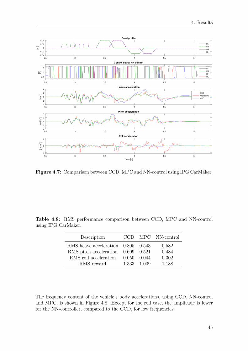
4. Results

2.5 3 3.5 4 4.5 5

-0.04

-0.02

0

0.02

0.04

[m]

Road profile

FL

FR

RR

RL

2.5 3 3.5 4 4.5 5

0.5

1

1.5

[A]

Control signal NN-control

FL

FR

RR

RL

2.5 3 3.5 4 4.5 5-4

-2

0

2

4

[m/s

2]

Heave acceleration

CCD

NN-control

MPC

2.5 3 3.5 4 4.5 5-4

-2

0

2

4

[rad/s

2]

Pitch acceleration

2.5 3 3.5 4 4.5 5

Time [s]

-2

0

2

[rad/s

2]

Roll acceleration

Figure 4.7: Comparison between CCD, MPC and NN-control using IPG CarMaker.

Table 4.8: RMS performance comparison between CCD, MPC and NN-controlusing IPG CarMaker.

Description CCD MPC NN-controlRMS heave acceleration 0.805 0.543 0.582RMS pitch acceleration 0.609 0.521 0.484RMS roll acceleration 0.050 0.044 0.302

RMS reward 1.333 1.009 1.188

The frequency content of the vehicle’s body accelerations, using CCD, NN-controland MPC, is shown in Figure 4.8. Except for the roll case, the amplitude is lowerfor the NN-controller, compared to the CCD, for low frequencies.

45

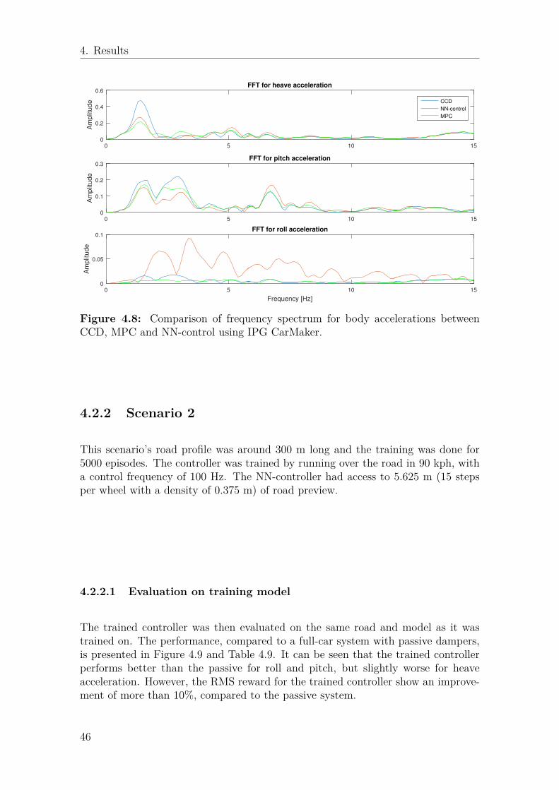
4. Results

0 5 10 150

0.2

0.4

0.6A

mp

litu

de

FFT for heave acceleration

CCD

NN-control

MPC

0 5 10 150

0.1

0.2

0.3

Am

plit

ud

e

FFT for pitch acceleration

0 5 10 15

Frequency [Hz]

0

0.05

0.1

Am

plit

ud

e

FFT for roll acceleration

Figure 4.8: Comparison of frequency spectrum for body accelerations betweenCCD, MPC and NN-control using IPG CarMaker.

4.2.2 Scenario 2

This scenario’s road profile was around 300 m long and the training was done for5000 episodes. The controller was trained by running over the road in 90 kph, witha control frequency of 100 Hz. The NN-controller had access to 5.625 m (15 stepsper wheel with a density of 0.375 m) of road preview.


The trained controller was then evaluated on the same road and model as it wastrained on. The performance, compared to a full-car system with passive dampers,is presented in Figure 4.9 and Table 4.9. It can be seen that the trained controllerperforms better than the passive for roll and pitch, but slightly worse for heaveacceleration. However, the RMS reward for the trained controller show an improve-ment of more than 10%, compared to the passive system.

46

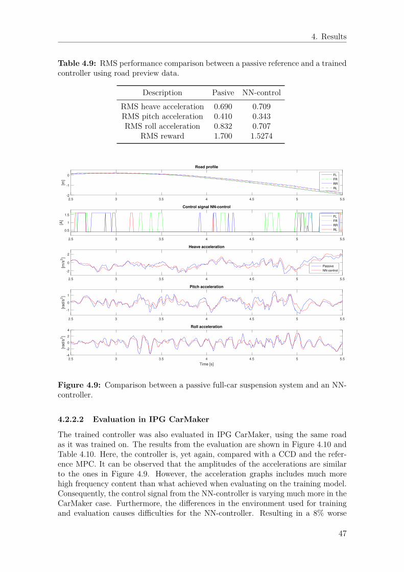
4. Results

Table 4.9: RMS performance comparison between a passive reference and a trainedcontroller using road preview data.

Description Pasive NN-controlRMS heave acceleration 0.690 0.709RMS pitch acceleration 0.410 0.343RMS roll acceleration 0.832 0.707

RMS reward 1.700 1.5274

2.5 3 3.5 4 4.5 5 5.5-2

-1

0

[m]

Road profile

FL

FR

RR

RL

2.5 3 3.5 4 4.5 5 5.5

0.5

1

1.5

[A]


FL

FR

RR

RL

2.5 3 3.5 4 4.5 5 5.5

-2

0

2

[m/s

2]

Heave acceleration

Passive

NN-control

2.5 3 3.5 4 4.5 5 5.5

-1

0

1

[rad/s

2]

Pitch acceleration

2.5 3 3.5 4 4.5 5 5.5

Time [s]

-4

-2

0

2

4

[rad/s

2]

Roll acceleration

Figure 4.9: Comparison between a passive full-car suspension system and an NN-controller.

4.2.2.2 Evaluation in IPG CarMaker

The trained controller was also evaluated in IPG CarMaker, using the same roadas it was trained on. The results from the evaluation are shown in Figure 4.10 andTable 4.10. Here, the controller is, yet again, compared with a CCD and the refer-ence MPC. It can be observed that the amplitudes of the accelerations are similarto the ones in Figure 4.9. However, the acceleration graphs includes much morehigh frequency content than what achieved when evaluating on the training model.Consequently, the control signal from the NN-controller is varying much more in theCarMaker case. Furthermore, the differences in the environment used for trainingand evaluation causes difficulties for the NN-controller. Resulting in a 8% worse

47

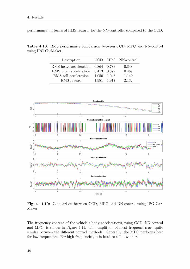
4. Results

performance, in terms of RMS reward, for the NN-controller compared to the CCD.

Table 4.10: RMS performance comparison between CCD, MPC and NN-controlusing IPG CarMaker.

Description CCD MPC NN-controlRMS heave acceleration 0.864 0.783 0.848RMS pitch acceleration 0.413 0.379 0.467RMS roll acceleration 1.050 1.048 1.140

RMS reward 1.981 1.917 2.132

2.5 3 3.5 4 4.5 5-2

-1

0

[m]

Road profile

FL

FR

RR

RL

2.5 3 3.5 4 4.5 5

0.5

1

1.5

[A]


FL

FR

RR

RL

2.5 3 3.5 4 4.5 5-4

-2

0

2

4

[m/s

2]

Heave acceleration

CCD

NN-control

MPC

2.5 3 3.5 4 4.5 5-2

0

2

[rad/s

2]

Pitch acceleration

2.5 3 3.5 4 4.5 5

Time [s]

-5

0

5

[rad/s

2]

Roll acceleration

Figure 4.10: Comparison between CCD, MPC and NN-control using IPG Car-Maker.

The frequency content of the vehicle’s body accelerations, using CCD, NN-controland MPC, is shown in Figure 4.11. The amplitude of most frequencies are quitesimilar between the different control methods. Generally, the MPC performs bestfor low frequencies. For high frequencies, it is hard to tell a winner.

48

4. Results

0 5 10 150

0.2

0.4

0.6A

mp

litu

de

FFT for heave acceleration

CCD

NN-control

MPC

0 5 10 150

0.1

0.2

Am

plit

ud

e

FFT for pitch acceleration

0 5 10 15

Frequency [Hz]

0

0.1

0.2

0.3

Am

plit

ud

e

FFT for roll acceleration

Figure 4.11: Comparison of frequency spectrum for body accelerations betweenCCD, MPC and NN-control using IPG CarMaker.

4.2.3 Scenario 3In this scenario the neural network specifications shown in Table 4.6 was used. Thisscenario’s road profile was around 150 m long and the training was done for 2300episodes. The controller was trained by running over the road in 30 kph, with acontrol frequency of 100 Hz. The NN-controller had access to 1.87 m (15 steps perwheel with a density of 0.1245 m) of road preview.


The trained controller was then evaluated on the same road and model as it wastrained on. The performance, compared to a full-car system with passive dampers,is presented in Figure 4.12 and Table 4.11. The trained controller shows good resultsfor all three accelerations. In total, the RMS reward for the trained controller showan improvement of more than 30%, compared to the passive system.

Table 4.11: RMS performance comparison between a passive reference and atrained controller using road preview data.

Description Passive NN-controlRMS heave acceleration 0.70 0.45RMS pitch acceleration 0.39 0.32RMS roll acceleration 0.13 0.09

RMS reward 1.07 0.75

49

4. Results

5 6 7 8 9 10 11 12 13 14 150

0.05

0.1

0.15

[m]

Road profile

FL

FR

RR

RL

5 6 7 8 9 10 11 12 13 14 15

0.5

1

1.5

[A]


FL

FR

RR

RL

5 6 7 8 9 10 11 12 13 14 15

-4

-2

0

2

4

[m/s

2]

Heave acceleration

Passive

NN-control

5 6 7 8 9 10 11 12 13 14 15

-2

0

2

[rad/s

2]

Pitch acceleration

5 6 7 8 9 10 11 12 13 14 15

Time [s]

-0.5

0

0.5

[rad/s

2]

Roll acceleration

Figure 4.12: Comparison between a passive full-car suspension system and anNN-controller.

4.2.4 Scenario 4In this scenario, continuous training was investigated and evaluated. A controllerwas trained on a 90 km long road, including mainly high frequency content. Thetraining time was approximately 60 h. The controller had a control frequency of 500Hz, in order to be able to handle the high frequency content. The controller wastrained by running over the road in 50 kph and had access to 5.625 m (15 steps perwheel with a density of 0.375 m) of road preview.


The trained controller was then evaluated on a short road with a similar shape asthe training road. The performance, compared to a full-car system with passivedampers, is presented in Figure 4.13 and Table 4.12. Because of the relatively smallhigh frequency noise, the heave and pitch accelerations are quite low for both con-trollers. The large accelerations occur in the roll spectrum and here the trainedcontroller significantly outperforms the passive reference. For the particular roadsegment, the improvement is 30% in terms of RMS roll acceleration. Speaking ofRMS reward, the trained controller show an improvement of a little more than 19%,compared to the passive system.

50

4. Results

Table 4.12: RMS performance comparison between a passive reference and atrained controller using road preview data.

Description Passive NN-controlRMS heave acceleration 0.93 0.91RMS pitch acceleration 0.95 0.92RMS roll acceleration 2.27 1.59

RMS reward 3.70 3.01

2 2.5 3 3.5 4 4.5 5 5.5 6

0.3

0.4

0.5

[m]

Road profile

FL

FR

RR

RL

2 2.5 3 3.5 4 4.5 5 5.5 6

0.5

1

1.5

[A]


FL

FR

RR

RL

2 2.5 3 3.5 4 4.5 5 5.5 6

-2

0

2

[m/s

2]

Heave acceleration

Passive

NN-control

2 2.5 3 3.5 4 4.5 5 5.5 6

-2

0

2

[rad/s

2]

Pitch acceleration

2 2.5 3 3.5 4 4.5 5 5.5 6

Time [s]

-5

0

5

[rad/s

2]

Roll acceleration

Figure 4.13: Comparison between a passive full-car suspension system and anNN-controller.

4.2.5 Execution timeCalculating the execution time for the controller is important to be able to see if it isfast enough to run in real-time. The execution time is the time it takes from sendingall the states as input to the controller/neural network, until achieving a controlsignal. In Figure 4.14, a histogram presents the distribution of the execution timesfor the NN-controller, collected from four different evaluations on two different roadprofiles. The simulations were run on a regular laptop and the controller consistedneural network with the architecture presented in Table 4.6. In the figure, it canbe observed that most of the execution times are less than 0.5 ms and almost allexecution times are less than 1 ms. This is just a fraction of the time that the

51

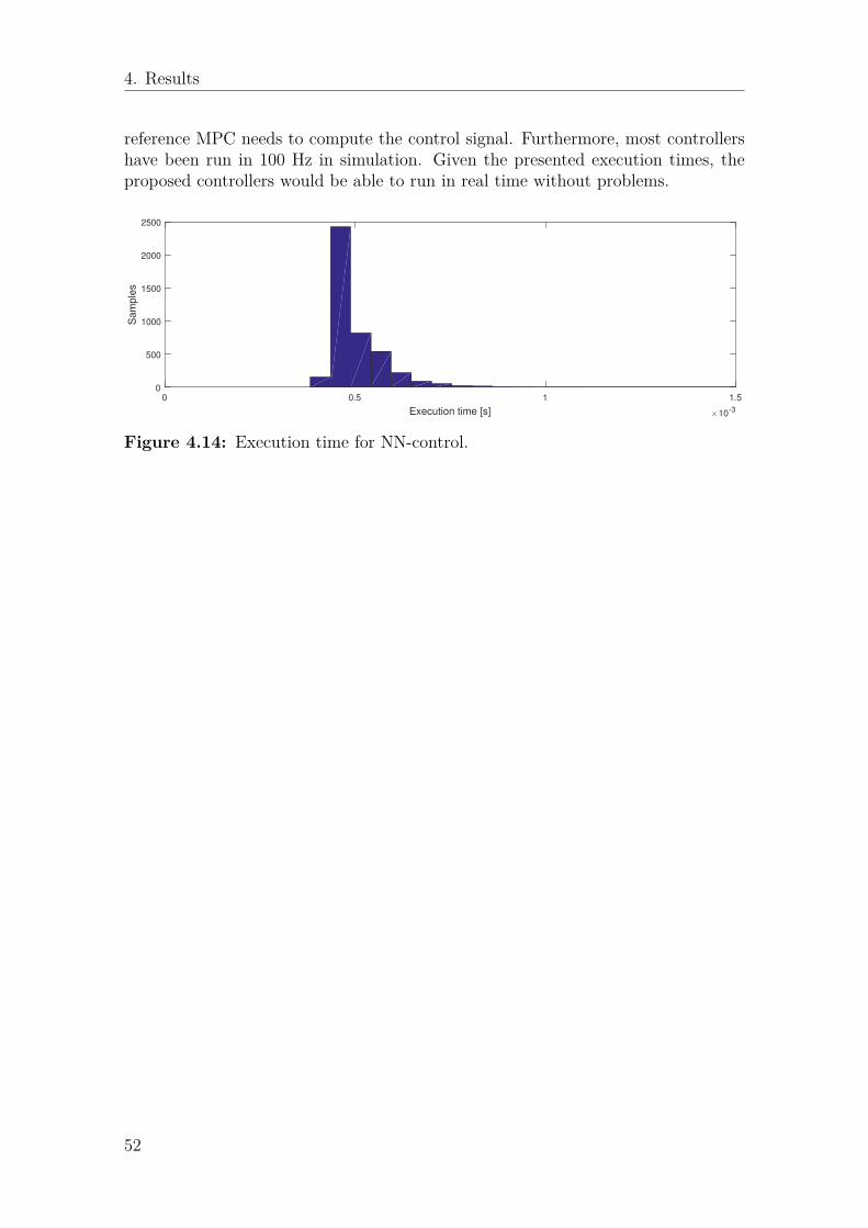
4. Results

reference MPC needs to compute the control signal. Furthermore, most controllershave been run in 100 Hz in simulation. Given the presented execution times, theproposed controllers would be able to run in real time without problems.

0 0.5 1 1.5

Execution time [s] ×10-3

0

500

1000

1500

2000

2500

Sa

mp

les

Figure 4.14: Execution time for NN-control.

52

5Discussion

The purpose of the thesis was to investigate if a neural network, trained by theDDPG algorithm, could be successful in controlling a full-car semi-active wheelsuspension system with access to road preview. To get a first indication of howthe DDPG algorithm would perform in a suspension system environment, a simplequarter-car model was designed and used for training. The results from traininga neural network, with the DDPG in the quarter-car environment, show that theDDPG successfully can train a controller to perform better than passive suspensionin the environment it has been trained on. Thereof, a more complex full-car modelwas designed to be used for further training. The results from training in the full-car environment shows that a neural network can control a semi-active suspensionsystem, and reach a performance that is significantly better than the performance ofa passive system. Furthermore, the neural network controller has also shown betterperformance than the reactive CCD controller that is used in today’s cars. Asidefrom investigating the performance of a neural network controller for semi-activewheel suspension, the computational complexity was said to be investigated. Theproposed controller has a relatively low computational complexity, just a fractionof the complexity of the reference MPC. Finally, the purpose of the thesis was toinvestigate the effect of using road preview in combination with a neural networkcontroller. The results showed that road preview speeds up training of the neuralnetwork, and that a higher performance can be reached.

The results show that episodic training on a road profile implies successful per-formance on the current road. By running over the same road for several times, thelearning converges to a satisfying control policy. Good performance for this taskcan be reached with rather small neural networks. Hence, a small computationalcost can be maintained. Evaluation of the trained neural networks controllers onother roads than the training road, has not been very successful. It was shown thatthe trained controllers could perform good on roads that had a similar shape, interms of frequency and magnitude, as the training road. Given very different roadscompared to the training road, the neural network controllers could not achievesatisfying results. This behaviour is however somewhat expected, since a trainedneural network controller will just perform good given similar states to what it hasvisited during training. Thus, to attain a single neural network controller that isable to perform well on all kinds of road profiles that can occur in practice, a neuralnetwork needs to be trained on a road profile that makes the full-car model visita much larger part on the entire state space. Further, for a neural network to beable to deliver suitable control signals for such a large state space, a deeper neural

53

5. Discussion

network that is trained for a longer time is probably needed. Because of the lowcomputational cost of the neural network used in this thesis, it is possible to makethe neural network much deeper without sacrificing the possibility to run in real time.

The performance of the neural network controllers was evaluated in terms of RMSroll, pitch and heave accelerations. By comparing the results for the different roadprofiles, it is clear that the learning algorithm develops different policies for dif-ferent road profiles. The learning algorithm finds what is the most optimal wayof maximizing its reward for the current road profile, which can be very differentdepending on the road. Since the reward is the negative sum of the roll, pitch andheave accelerations, the algorithm will often focus on reducing one or two of theaccelerations if it results in a better reward. This behaviour is probably not desiredfor a controller in a real car, but it can easily be changed by changing the rewardfunction. The performance in terms of different frequencies shows that the neuralnetwork controller generally performs good for low frequencies (primary ride) andworse for high frequencies (secondary ride). Whether this behaviour can be changedby changing the reward, or if it is due to something else is unclear.

As mentioned previously, the calculated execution times for the neural networkto compute the control signal is just a fraction of the time the reference MPC needs.Further, the execution times for neural networks does not vary with different inputsets of data. This is not the case for the MPC, which is very dependent on thecomputational complexity from the given inputs. Hence, neural networks might bemore suitable than MPC to be used in a real-time system, where the inputs variessubstantially.

The road preview data that is sent to the controller has not been optimized in termsof preview length and density. A couple of different setups were tried during theprocess, but it is definitely an area that can be improved further. By increasing thesize of the preview data (either by increasing the preview length or the density), theobservation state space that the controller needs to map increases rapidly. Hence,even though an increased preview size could improve the performance slightly, butit may not be the optimal way of spending the computational resources that areavailable.

Regarding the DDPG learning algorithm, it has shown to be successful for learningin the environment of interest. It can learn a successful policy in a continuous stateand action space, given an arbitrary reward to represent ride comfort.

5.1 ConclusionIn this thesis, a control approach for semi-active wheel suspension with road previewhas been proposed. The control approach is based on an artificial neural networktrained with reinforcement learning, more specifically the DDPG algorithm. The

54

5. Discussion

learning method has shown to be successful in both continuous and episodic envi-ronments. The approach shows promising results, often able to outperform today’sCCD controller for semi-active suspension in simulation. The trained controller doesnot really match the performance of the reference MPC, but the computational costof the trained controller is just a fraction. This indicates that the proposed controlapproach can be further improved by utilizing a deeper neural network.

5.2 Future workTo achieve a controller that is suitable for all kind of road profiles, a neural networkneeds to be trained on a road that covers a much larger space of the entire statespace. In order for the network to collect all information during the training, adeeper network should be considered. Alternatively one could train several differentnetworks and change between the networks depending on the road. Furthermore,the road preview should be optimized in terms of preview length and density. Also,to be able to run on a real car, rotational pre-processing of the road preview datais needed to suit a camera on top of the car.

55

5. Discussion

56

References

[1] Y. Zhou and S. Chen, “Vehicle ride comfort analysis with whole-body vibrationon long-span bridges subjected to crosswind”, Journal of Wind Engineeringand Industrial Aerodynamics, vol. 155, pp. 126 –140, 2016, issn: 0167-6105.doi: https://doi.org/10.1016/j.jweia.2016.05.001.

[2] P. Els, N. Theron, P. Uys, and M. Thoresson, “The ride comfort vs. handlingcompromise for off-road vehicles”, Journal of Terramechanics, vol. 44, no. 4,pp. 303 –317, 2007, issn: 0022-4898. doi: https://doi.org/10.1016/j.jterra.2007.05.001.

[3] F. Kjellberg and S. Sundell, “Real-time nonlinear model predictive controlfor semi-active suspension with road preview”, M.S. thesis, Department ofElectrical Engineering, Chalmers University of Technology, Gothenburg, Swe-den, 2018. [Online]. Available: http://publications.lib.chalmers.se/records/fulltext/255751/255751.pdf.

[4] M. Willis, G. Montague, C. D. Massimo, M. Tham, and A. Morris, “Artificialneural networks in process estimation and control”, Automatica, vol. 28, no. 6,pp. 1181 –1187, 1992, issn: 0005-1098. doi: https://doi.org/10.1016/0005-1098(92)90059-O.

[5] J. MacMurray and D. Himmelblau, “Identification of a packed distillationcolumn for control via artificial neural networks”, in 1993 American ControlConference, 1993, pp. 1455–1459. doi: 10.23919/ACC.1993.4793112.

[6] J. Thibault and B. Grandjean, “Neural networks in process control - a survey”,in Advanced Control of Chemical Processes 1991, ser. IFAC Symposia Series,K. NAJIM and E. DUFOUR, Eds., Amsterdam: Pergamon, 1992, pp. 251 –260, isbn: 978-0-08-041267-2. doi: https://doi.org/10.1016/B978-0-08-041267-2.50046-2.

[7] M. T. Hagan, H. B. Demuth, and O. D. Jesús, “An introduction to the useof neural networks in control systems”, International Journal of Robust andNonlinear Control, vol. 12, no. 11, pp. 959–985, 2002. doi: 10.1002/rnc.727.

[8] N. Casas, “Deep deterministic policy gradient for urban traffic light control”,CoRR, 2017. [Online]. Available: http://arxiv.org/abs/1703.09035.

[9] A. Kumar, N. Paul, and S. N. Omkar, “Bipedal walking robot using deep de-terministic policy gradient”, CoRR, 2018. [Online]. Available: http://arxiv.org/abs/1807.05924.

57

https://doi.org/https://doi.org/10.1016/j.jweia.2016.05.001

https://doi.org/https://doi.org/10.1016/j.jterra.2007.05.001

https://doi.org/https://doi.org/10.1016/j.jterra.2007.05.001

http://publications.lib.chalmers.se/records/fulltext/255751/255751.pdf


https://doi.org/https://doi.org/10.1016/0005-1098(92)90059-O

https://doi.org/https://doi.org/10.1016/0005-1098(92)90059-O

https://doi.org/10.23919/ACC.1993.4793112

https://doi.org/https://doi.org/10.1016/B978-0-08-041267-2.50046-2

https://doi.org/https://doi.org/10.1016/B978-0-08-041267-2.50046-2

https://doi.org/10.1002/rnc.727

http://arxiv.org/abs/1703.09035



References

[10] G. Cano Lopes, M. Ferreira, A. Simões, and E. Luna Colombini, “Intelligentcontrol of a quadrotor with proximal policy optimization reinforcement learn-ing”, Nov. 2018, pp. 503–508. doi: 10.1109/LARS/SBR/WRE.2018.00094.

[11] J. Hwangbo, I. Sa, R. Siegwart, and M. Hutter, “Control of a quadrotor withreinforcement learning”, IEEE Robotics and Automation Letters, vol. 2, no. 4,pp. 2096–2103, 2017, issn: 2377-3766. doi: 10.1109/LRA.2017.2720851.

[12] T. P. Lillicrap, J. J. Hunt, A. Pritzel, N. Heess, T. Erez, Y. Tassa, D. Silver, andD. Wierstra, “Continuous control with deep reinforcement learning”, CoRR,vol. abs/1509.02971, 2015. [Online]. Available: http://arxiv.org/abs/1509.02971.

[13] V. Mnih, K. Kavukcuoglu, D. Silver, A. Graves, I. Antonoglou, D. Wierstra,and M. A. Riedmiller, “Playing atari with deep reinforcement learning”, CoRR,vol. abs/1312.5602, 2013. [Online]. Available: https://arxiv.org/abs/1312.5602.

[14] M. Tomizuka, ““optimum linear preview control with application to vehi-cle suspension”—revisited”, Journal of Dynamic Systems Measurement andControl-transactions of The Asme - J DYN SYST MEAS CONTR, vol. 98,Sep. 1976. doi: 10.1115/1.3427040.

[15] A G. Thompson, B R. Davis, and C E. M. Pearce, “An optimal linear ac-tive suspension with finite road preview”, in 1980 Automotive EngineeringCongress and Exposition, Feb. 1980. doi: 10.4271/800520.

[16] G. Prokop and R. Sharp, “Performance enhancement of limited-bandwidthactive automotive suspensions by road preview”, Control Theory and Applica-tions, IEE Proceedings, vol. 142, pp. 140 –148, Apr. 1995. doi: 10.1049/ip-cta:19951772.

[17] R. Mehra, J. Amin, K. Hedrick, C Osorio, and S Gopalasamy, “Active sus-pension using preview information and model predictive control”, Nov. 1997,pp. 860 –865. doi: 10.1109/CCA.1997.627769.

[18] C. Göhrle, A. Schindler, A. Wagner, and O. Sawodny, “Model predictive con-trol of semi-active and active suspension systems with available road preview”,pp. 1499–1504, 2013. doi: 10.23919/ECC.2013.6669185.

[19] C. Göhrle, A. Schindler, A. Wagner, and O. Sawodny, “Road profile esti-mation and preview control for low-bandwidth active suspension systems”,IEEE/ASME Transactions on Mechatronics, vol. 20, no. 5, pp. 2299–2310,2015, issn: 1083-4435. doi: 10.1109/TMECH.2014.2375336.

[20] M. Q. Nguyen, M. Canale, O. Sename, and L. Dugard, “A model predictivecontrol approach for semi-active suspension control problem of a full car”, in2016 IEEE 55th Conference on Decision and Control (CDC), 2016, pp. 721–726. doi: 10.1109/CDC.2016.7798353.

[21] M. Howell, G. Frost, T. Gordon, and Q. Wu, “Continuous action reinforcementlearning applied to vehicle suspension control”, Mechatronics, vol. 7, no. 3,pp. 263 –276, 1997, issn: 0957-4158. doi: 10.1016/S0957-4158(97)00003-2.

58

https://doi.org/10.1109/LARS/SBR/WRE.2018.00094

https://doi.org/10.1109/LRA.2017.2720851



https://arxiv.org/abs/1312.5602

https://arxiv.org/abs/1312.5602

https://doi.org/10.1115/1.3427040

https://doi.org/10.4271/800520

https://doi.org/10.1049/ip-cta:19951772

https://doi.org/10.1049/ip-cta:19951772

https://doi.org/10.1109/CCA.1997.627769

https://doi.org/10.23919/ECC.2013.6669185

https://doi.org/10.1109/TMECH.2014.2375336

https://doi.org/10.1109/CDC.2016.7798353

https://doi.org/10.1016/S0957-4158(97)00003-2

References

[22] S. Tognetti, S. M. Savaresi, C. Spelta, and M. Restelli, “Batch reinforcementlearning for semi-active suspension control”, in 2009 IEEE Control Appli-cations, (CCA) Intelligent Control, (ISIC), Saint Petersburg, Russia, 2009.[Online]. Available: https://ieeexplore.ieee.org/stamp/stamp.jsp?arnumber=5281070.

[23] I. Bucak and H R. Öz, “Vibration control of a nonlinear quarter-car active sus-pension system by reinforcement learning”, International Journal of SystemsScience - IJSySc, vol. 43, pp. 1177–1190, Jun. 2012. doi: 10.1080/00207721.2010.549576.

[24] A. R. Bhise, R. G. Desai, R. N. Yerrawar, A. Mitra, and R. R. Arakerimath,“Comparison between passive and semi-active suspension system using mat-lab/simulink and serially concatenated codes”, IOSR Journal of Mechanicaland Civil Engineering, vol. 13, no. 4, pp. 01–06, 2016. [Online]. Available:http://iosrjournals.org/iosr-jmce/papers/vol13-issue4/Version-1/A1304010106.pdf.

[25] S. A. Hassan, “Fundamental studies of passive, active and semi-active auto-motive suspension systems”, Ph.D. dissertation, Department of MechanicalEngineering, The University of Leeds, Leeds, UK, 1986. [Online]. Available:https://core.ac.uk/download/pdf/9257269.pdf.

[26] M. A. Nekoui and P. Hadavi, “Optimal control of an active suspension system”,in Proceedings of 14th International Power Electronics and Motion ControlConference EPE-PEMC 2010, Ohrid, Macedonia, 2010.

[27] A. F. Mohd Riduan, N. Tamaldin, A. Sudrajat, and F. Ahmad, “Review onactive suspension system”, SHS Web of Conferences, vol. 49, p. 02 008, 2018.doi: 10.1051/shsconf/20184902008.

[28] N. Ito, “Semi-active suspension”, in KYB Technical review, T. Tezuka et al,Ed., Tokyo, Japan: Shobi Printing Co., 2017, pp. 31 –32. [Online]. Available:https://www.kyb.co.jp/english/technical_report/data/no55e/all.pdf.

[29] M. Witters and J. Swevers, “Identification of noe models for a continuouslyvariable semi-active damper”, 23rd International Conference on Noise andVibration Engineering 2008, ISMA 2008, vol. 7, Jan. 2008.

[30] J. Reimpell, H. Stoll, and J. W. Betzler, in The Automotive Chassis, SecondEdition, Oxford: Butterworth-Heinemann, 2001, isbn: 978-0-7506-5054-0.

[31] K. Wolff, J. Hoppermans, and R. Kraaijeveld, “Objective evaluation of sub-jective driving impressions”, JSAE Annual Cong, Yokohama, Japan, 2008.[Online]. Available: https : / / www . fev . com / fileadmin / user _ upload /Media/TechnicalPublications/Chassis/V0815_FISITA2008_Objective_Evaluation_F20080319-Paper_01.pdf.

[32] R. Dixon, “Back to basics – ride quality and comfort”, Motorworld Media,Oct. 26, 2014. [Online]. Available: http://www.dieselcar.com/features/doctor/back-to-basics-ride-quality-and-comfort/.

59

https://ieeexplore.ieee.org/stamp/stamp.jsp?arnumber=5281070

https://ieeexplore.ieee.org/stamp/stamp.jsp?arnumber=5281070

https://doi.org/10.1080/00207721.2010.549576

https://doi.org/10.1080/00207721.2010.549576

http://iosrjournals.org/iosr-jmce/papers/vol13-issue4/Version-1/A1304010106.pdf

http://iosrjournals.org/iosr-jmce/papers/vol13-issue4/Version-1/A1304010106.pdf

https://core.ac.uk/download/pdf/9257269.pdf

https://doi.org/10.1051/shsconf/20184902008

https://www.kyb.co.jp/english/technical_report/data/no55e/all.pdf

https://www.kyb.co.jp/english/technical_report/data/no55e/all.pdf

https://www.fev.com/fileadmin/user_upload/Media/TechnicalPublications/Chassis/V0815_FISITA2008_Objective_Evaluation_F20080319-Paper_01.pdf



http://www.dieselcar.com/features/doctor/back-to-basics-ride-quality-and-comfort/

http://www.dieselcar.com/features/doctor/back-to-basics-ride-quality-and-comfort/

References

[33] A. Kruczek and A. Stribrsky, “A full-car model for active suspension - somepractical aspects”, in Proceedings of the IEEE International Conference onMechatronics, 2004. ICM ’04., 2004, pp. 41–45. doi: 10.1109/ICMECH.2004.1364409.

[34] S. M. Savaresi, C. Poussot-Vassal, C. Spelta, O. Sename, and L. Dugard,“Chapter 3 - suspension oriented vehicle models”, in Semi-Active SuspensionControl Design for Vehicles, Boston, USA: Butterworth-Heinemann, 2010,pp. 41 –69, isbn: 978-0-08-096678-6. [Online]. Available: http://www.sciencedirect.com/science/article/pii/B9780080966786000031.

[35] R. N. Jazar,Vehicle Dynamics: Theory and Applications. Riverdale, NY: SpringerScience+Business Media, 2008, isbn: 978-0-387-74243-4.

[36] J. D. Seo, “My journey to reinforcement learning — part 0: Introduction”, To-wards Data Science, Apr. 7, 2018. [Online]. Available: https://towardsdatascience.com/my-journey-to-reinforcement-learning-part-0-introduction-1e3aec1ee5bf.

[37] ADL, “A brief introduction to reinforcement learning”, Medium, Aug. 27,2018. [Online]. Available: https://medium.freecodecamp.org/a-brief-introduction-to-reinforcement-learning-7799af5840db.

[38] R. S. Sutton and A. G. Barto, Reinforcement Learning: An Introduction,2nd ed. Cambridge, Massachusetts: The MIT Press, 2018, isbn: 978-0-26-203924-6.

[39] J. Hui, “Rl—model-based reinforcement learning”, Medium, Sep. 25, 2018.[Online]. Available: https://medium.com/@jonathan_hui/rl-model-based-reinforcement-learning-3c2b6f0aa323.

[40] T. Xia and Z. Han, “Path planning using reinforcement learning and ob-jective data”, M.S. thesis, Department of Computer Science and Engineer-ing, Chalmers University of Technology, Gothenburg, Sweden, 2017. [Online].Available: http://publications.lib.chalmers.se/records/fulltext/256451/256451.pdf.

[41] C. J.C. H. Watkins and P. Dayan, “Q-learning”, Machine Learning, vol. 8,no. 3, pp. 279–292, 1992, issn: 1573-0565. doi: 10.1007/BF00992698.

[42] A. Juliani, “Simple reinforcement learning with tensorflow part 4: Deep q-networks and beyond”, Medium, Sep. 2, 2016. [Online]. Available: https :/ / medium . com / @awjuliani / simple - reinforcement - learning - with -tensorflow-part-4-deep-q-networks-and-beyond-8438a3e2b8df.

[43] T. Simonini, “An introduction to policy gradients with cartpole and doom”,Medium, May 9, 2018. [Online]. Available: https://medium.freecodecamp.org/an-introduction-to-policy-gradients-with-cartpole-and-doom-495b5ef2207f.

[44] D. Silver, G. Lever, N. Heess, T. Degris, D. Wierstra, and M. Riedmiller,“Deterministic policy gradient algorithms”, 31st International Conference onMachine Learning, ICML 2014, vol. 1, Jun. 2014.

60

https://doi.org/10.1109/ICMECH.2004.1364409

https://doi.org/10.1109/ICMECH.2004.1364409

http://www.sciencedirect.com/science/article/pii/B9780080966786000031

http://www.sciencedirect.com/science/article/pii/B9780080966786000031

https://towardsdatascience.com/my-journey-to-reinforcement-learning-part-0-introduction-1e3aec1ee5bf



https://medium.freecodecamp.org/a-brief-introduction-to-reinforcement-learning-7799af5840db

https://medium.freecodecamp.org/a-brief-introduction-to-reinforcement-learning-7799af5840db

https://medium.com/@jonathan_hui/rl-model-based-reinforcement-learning-3c2b6f0aa323

https://medium.com/@jonathan_hui/rl-model-based-reinforcement-learning-3c2b6f0aa323



https://doi.org/10.1007/BF00992698

https://medium.com/@awjuliani/simple-reinforcement-learning-with-tensorflow-part-4-deep-q-networks-and-beyond-8438a3e2b8df



https://medium.freecodecamp.org/an-introduction-to-policy-gradients-with-cartpole-and-doom-495b5ef2207f



References

[45] E. Bibbona, G. Panfilo, and P. Tavella, “The ornstein–uhlenbeck process as amodel of a low pass filtered white noise”, Metrologia, vol. 45, Dec. 2008. doi:10.1088/0026-1394/45/6/S17.

[46] K. Mohiuddin, J. Mao, and A. K. Jain, “Artificial neural networks: A tutorial”,Computer, vol. 29, pp. 31–44, Mar. 1996, issn: 0018-9162. doi: 10.1109/2.485891.

[47] L. Dormehl, “What is an artificial neural network? here’s everything youneed to know”, Digital Trends, Jan. 5, 2019. [Online]. Available: https://www.digitaltrends.com/cool-tech/what-is-an-artificial-neural-network/.

[48] A. Sharma, “Understanding activation functions in neural networks”, Medium,Mar. 30, 2017. [Online]. Available: https : / / medium . com / the - theory -of - everything / understanding - activation - functions - in - neural -networks-9491262884e0.

[49] P. Emami, “Deep deterministic policy gradients in tensorflow”, My summariesof Machine Learning papers and investigations into various topics concerningartificial intelligence, Aug. 2016. [Online]. Available: https://pemami4911.github.io/blog/2016/08/21/ddpg-rl.html.

61

https://doi.org/10.1088/0026-1394/45/6/S17

https://doi.org/10.1109/2.485891

https://doi.org/10.1109/2.485891

https://www.digitaltrends.com/cool-tech/what-is-an-artificial-neural-network/



https://medium.com/the-theory-of-everything/understanding-activation-functions-in-neural-networks-9491262884e0



https://pemami4911.github.io/blog/2016/08/21/ddpg-rl.html

https://pemami4911.github.io/blog/2016/08/21/ddpg-rl.html

References

62

neuralnetworkcontrollerforsemi-active suspension systems with … · 2019-07-09 ·...

Documents