neural dynamics in cortical populations - ucl...
TRANSCRIPT

Neural dynamics in corticalpopulations
Marius Pachitariu
Dissertation submitted for the degree ofDoctor of Philosophy
ofUniversity College London
Gatsby Computational Neuroscience Unit
University College London
2014

Declaration
I, Marius Pachitariu, declare that this thesis was composed bymyself, that the work contained herein is my own except whereexplicitly stated otherwise in the text, and that this work has notbeen submitted for any other degree or professional qualificationexcept as specified.
Marius PachitariuJanuary 30, 2015
Abstract
Many essential neural computations are implemented by large popula-tions of neurons working in concert. Recent studies have sought bothto monitor increasingly large groups of neurons and to characterise theircollective behaviour, but the standard computational approaches avail-able to identify the collective dynamics scale poorly with the size ofthe dataset. We develop new efficient methods for discovering the low-dimensional dynamics that underlie simultaneously-recorded spike trainsfrom a neural population. We use the new models to analyze two differentsets of population recordings, one from motor cortex and another fromauditory cortex. In motor cortex, we describe the nature of the trial-by-trial spontaneous fluctuations identified by the model and connect thesefluctuations to behavioral events. The spatio-temporal structure of thespontaneous events was tracked by three trajectories identified by themodel. These trajectories followed similar dynamics during hand reachesas they did when the hands were stationary. The structure of the mod-els we developed allow them to be used as decoders of hand positionfrom neural activity, significantly improving upon previous state-of-the-art methods. The decoders were able to predict information about thedirection, onset time and speed profile of movements. In auditory cortex,we use the statistical models to identify population dynamics under dif-ferent brain states. We report major differences in dynamics and stimuluscoding between synchronized and desychronized brain states. Synchro-nized but not desynchronized brain states imposed constraints on neuraldynamics such that a four-dimensional system accounted for most of thedynamical structure of population events. We used the low-dimensionalrepresentation of the data to construct network simulations that repro-duced the patterns present in the recordings. The simulations suggestthat the overall level of feedback inhibition controls the stability of eachlocal cortical network, with unstable dynamics resulting in synchronizedbrain states. Finally we propose a functional role for dynamics in therepresentation of visual motion in visual cortex.
Acknowledgments
I thank my supervisor Maneesh Sahani for the guidance and all the help he hasprovided over the years, and for the connections he has helped me build withother theoretical and experimental researchers.
I thank Peter Dayan for holding the Gatsby Unit together and on a steady coursewhile supporting the diversity of research conducted there. I thank Peter Latham,Yee Whye Teh and Arthur Gretton for providing different viewpoints into science,and I thank my fellow Gatsby colleagues, the students and postdocs with whomI shared my academic and social endeavours. I have started my studies alongsideArthur Guez and I thank him for his camaraderie and for keeping a good pace inthe marathon that has been the Gatsby PhD.
I thank my experimental collaborators outside the Gatsby Unit, that have givenme practical views into scientific life as well as access to their hard-earned data.They have been a model for me and a continuous source of interesting discussion,helping me shape my armchair analytic thinking to the practical problems ofscientific experimentation. At the Ear Institute I have collaborated closely withNicholas Lesica, who has significantly extended my scientific interests. At theCruciform I have collaborated with Adam Packer and other members of MichaelHausser’s laboratory and I also had the opportunity to work closely with ThomasMrsic-Flogel, Sonja Hofer, Adil Khan, Jasper Poort and other members of theirgroup. I also thank my collaborators outside London, Krishna Shenoy and mem-bers of his lab in Stanford.
Outside of academia, my family has been a constant source of support and sohave my friends from Princeton and those from my hometown. Carsen also hasbeen a great source of moral support as well as academic help during the finalyear of my doctorate.

Contents
Declaration . . . . . . . . . . . . . . . . . . . . . . . . . . . . . . . . . . 2Abstract . . . . . . . . . . . . . . . . . . . . . . . . . . . . . . . . . . . . 3Acknowledgments . . . . . . . . . . . . . . . . . . . . . . . . . . . . . . . 4Table of contents . . . . . . . . . . . . . . . . . . . . . . . . . . . . . . . 5List of figures . . . . . . . . . . . . . . . . . . . . . . . . . . . . . . . . . 8Outline . . . . . . . . . . . . . . . . . . . . . . . . . . . . . . . . . . . . 10
1 Introduction 111.1 An informal introduction to the study of brain dynamics . . . . . . 121.2 Collective behavior in networks of neurons . . . . . . . . . . . . . . 141.3 Four types of state-dependent patterns in cortical recordings . . . 161.4 Multi-purpose dynamical models . . . . . . . . . . . . . . . . . . . 17
2 Recurrent linear models of simultaneously-recorded neural pop-ulations 232.1 Introduction . . . . . . . . . . . . . . . . . . . . . . . . . . . . . . . 242.2 From Kalman filters to recurrent linear models . . . . . . . . . . . 252.3 Recurrent linear models with Poisson observations . . . . . . . . . 28
2.3.1 Relationship to other models . . . . . . . . . . . . . . . . . 292.4 Cascaded linear models . . . . . . . . . . . . . . . . . . . . . . . . 312.5 Alternative models . . . . . . . . . . . . . . . . . . . . . . . . . . . 33
2.5.1 Alternative for temporal interactions: causally-coupledgeneralized linear model . . . . . . . . . . . . . . . . . . . . 33
2.5.2 Alternative for instantaneous interactions: the Ising model 342.6 Results . . . . . . . . . . . . . . . . . . . . . . . . . . . . . . . . . . 36
2.6.1 Simulated data . . . . . . . . . . . . . . . . . . . . . . . . . 362.6.2 Array recorded data . . . . . . . . . . . . . . . . . . . . . . 37
2.7 Discussion . . . . . . . . . . . . . . . . . . . . . . . . . . . . . . . . 39
3 Recurrent linear analysis of multi-neuron recordings from motorcortex 413.1 Neural dynamics in motor cortex . . . . . . . . . . . . . . . . . . . 423.2 Statistical models of delay-period activity extract consistent single-
trial patterns . . . . . . . . . . . . . . . . . . . . . . . . . . . . . . 443.3 Delay period shared fluctuations are associated with micro-
movements . . . . . . . . . . . . . . . . . . . . . . . . . . . . . . . 46

0 CONTENTS 6
3.4 Fluctuations in M1 activity align with population patterns duringmovement . . . . . . . . . . . . . . . . . . . . . . . . . . . . . . . . 47
3.5 Stimulus and movement onset drastically reduce mutual informa-tion in M1 . . . . . . . . . . . . . . . . . . . . . . . . . . . . . . . . 48
3.6 Comparison with noise correlation analysis . . . . . . . . . . . . . 503.7 The fine details of movements are encoded by motor cortex . . . . 513.8 What information from the population spiking does the decoder use? 52
4 Quiescence in neural circuits enhances coding of continuous sen-sory streams 584.1 Fluctuations exist and can be quenched in active states . . . . . . 59
4.1.1 Hypothesis of unstable network activity . . . . . . . . . . . 594.1.2 Fluctuating states do not code well in ongoing stimulation,
but quiescent states do . . . . . . . . . . . . . . . . . . . . . 614.1.3 Possible mechanisms underlying quiescent states . . . . . . 614.1.4 Intracellular voltages . . . . . . . . . . . . . . . . . . . . . . 64
4.2 Deterministic network model reproduces the inherent randomnessof fluctuations . . . . . . . . . . . . . . . . . . . . . . . . . . . . . . 644.2.1 Inhibition stabilizes network activity . . . . . . . . . . . . . 66
4.3 Quiescence enables sharp tuning, high-dimensional stimulus re-sponse and temporal integration . . . . . . . . . . . . . . . . . . . 66
4.4 Conclusion . . . . . . . . . . . . . . . . . . . . . . . . . . . . . . . 684.5 Methods . . . . . . . . . . . . . . . . . . . . . . . . . . . . . . . . . 69
4.5.1 Integrate-and-Fire Network . . . . . . . . . . . . . . . . . . 69
5 Recurrent linear analysis of state-dependent A1 population ac-tivity 715.1 Cortical states . . . . . . . . . . . . . . . . . . . . . . . . . . . . . 725.2 Model performance . . . . . . . . . . . . . . . . . . . . . . . . . . . 745.3 The phenomenology of dynamics . . . . . . . . . . . . . . . . . . . 755.4 Fluctuating states in awake-passive recordings . . . . . . . . . . . . 795.5 Four-dimensional reduced simulation of network states . . . . . . . 82
6 State-dependent population coding in primary auditory cortex 886.1 Introduction . . . . . . . . . . . . . . . . . . . . . . . . . . . . . . . 896.2 Synchronized and desynchronized states in A1 . . . . . . . . . . . . 906.3 The impact of cortical state on responses to tones . . . . . . . . . 926.4 The impact of cortical state on the temporal precision and relia-
bility of responses to speech . . . . . . . . . . . . . . . . . . . . . . 946.5 The impact of cortical state on the similarity of spike patterns
evoked by different speech tokens . . . . . . . . . . . . . . . . . . 966.6 The impact of cortical state on noise correlations and population
decoding . . . . . . . . . . . . . . . . . . . . . . . . . . . . . . . . . 1006.7 Spike patterns evoked by different speech tokens in synchronized
A1 are similar and have strong noise correlations even within upstates . . . . . . . . . . . . . . . . . . . . . . . . . . . . . . . . . . 102
6.8 Differences between synchronized and desynchronized states in thesame population . . . . . . . . . . . . . . . . . . . . . . . . . . . . 105
0 CONTENTS 7
6.9 Discussion . . . . . . . . . . . . . . . . . . . . . . . . . . . . . . . . 1076.10 Materials and Methods . . . . . . . . . . . . . . . . . . . . . . . . . 110
7 Learning visual motion in recurrent neural networks 1167.1 Introduction . . . . . . . . . . . . . . . . . . . . . . . . . . . . . . . 117
7.1.1 Recurrent Network Models for Neural Sequence Learning. . 1187.2 Linear neurons with recurrent connectivity enable history-
dependent computations . . . . . . . . . . . . . . . . . . . . . . . . 1197.2.1 Complexity order for recurrent networks versus feedforward
filters . . . . . . . . . . . . . . . . . . . . . . . . . . . . . . 1267.3 Probabilistic Recurrent Neural Networks . . . . . . . . . . . . . . . 128
7.3.1 Binary Gated Gaussian Sparse Coding (bgG-SC). . . . . . . 1297.3.2 Binary-Gated Gaussian Recurrent Neural Network (bgG-
RNN). . . . . . . . . . . . . . . . . . . . . . . . . . . . . . . 1317.3.3 Inference and learning of bgG-RNN. . . . . . . . . . . . . . 132
7.4 Results . . . . . . . . . . . . . . . . . . . . . . . . . . . . . . . . . . 1337.4.1 Measuring responses in the model. . . . . . . . . . . . . . . 1347.4.2 Direction selectivity and speed tuning. . . . . . . . . . . . 1347.4.3 Vector velocity tuning . . . . . . . . . . . . . . . . . . . . . 1377.4.4 Connectomics in silico . . . . . . . . . . . . . . . . . . . . . 137
7.5 Discussion . . . . . . . . . . . . . . . . . . . . . . . . . . . . . . . . 139
8 Conclusion 1438.1 Emerging technologies for large-scale recordings . . . . . . . . . . . 147
References 150

List of figures
1.1 Recurrent linear models can recover underlying dynamicsfrom data . . . . . . . . . . . . . . . . . . . . . . . . . . . . . . . 18
1.2 Multi-purpose hidden Markov dynamical models . . . . . . 20
2.1 Hidden Markov dynamical systems . . . . . . . . . . . . . . . 272.2 Experiments on simulated data with RLM framework . . . 352.3 RLM performance on array-recorded data from monkey
M1 . . . . . . . . . . . . . . . . . . . . . . . . . . . . . . . . . . . 372.4 Samples from cascaded linear model . . . . . . . . . . . . . . 392.5 Samples drawn from the model distribution . . . . . . . . . 402.6 RLM with low-dimensional PSTH model . . . . . . . . . . . 40
3.1 Example multi-neuron recording in motor cortex . . . . . . 433.2 Model structure . . . . . . . . . . . . . . . . . . . . . . . . . . . 453.3 Trial-by-trial variability in the delay period . . . . . . . . . 543.4 Movement slips in the delay period correlate with neural
events . . . . . . . . . . . . . . . . . . . . . . . . . . . . . . . . . . 553.5 Single-trial decoding during reaches . . . . . . . . . . . . . . 563.6 Effect of perturbations on decoder . . . . . . . . . . . . . . . 57
4.1 Quiescent states respond reliably to continuous streamsof sound . . . . . . . . . . . . . . . . . . . . . . . . . . . . . . . . 60
4.3 Potential mechanisms for quiescent states: inhibition,adaptation and EPSP amplitude . . . . . . . . . . . . . . . . . 63
4.4 Increased inhibition reproduces transition from fluctuat-ing to quiescent states in network simulation . . . . . . . . . 65
4.5 Quiescent states enable network to use high dimensionsfor coding . . . . . . . . . . . . . . . . . . . . . . . . . . . . . . . 67
5.1 Cortical state varies throughout experiments and substan-tially affects the multi-neuron patterns recorded . . . . . . 73
5.2 Recurrent linear model predictive performance, comparedwith GLMs . . . . . . . . . . . . . . . . . . . . . . . . . . . . . . 75
5.3 Example trajectories in spontaneous activity . . . . . . . . . 765.4 Spike sequences are captured by RLM trajectories . . . . . 78

0 LIST OF FIGURES 9
5.5 Dynamical models capture fluctuating states and their pe-riodicity . . . . . . . . . . . . . . . . . . . . . . . . . . . . . . . . 79
5.6 Fentanyl to Urethane pattern transitions . . . . . . . . . . . 815.7 Schematic of low-d model . . . . . . . . . . . . . . . . . . . . . 825.8 Low-d simulated dynamics of cortical states . . . . . . . . . 855.9 Nullcline dynamics of synchronized states . . . . . . . . . . . 865.10 Stimulus onset reduces variability in synchronized states . 865.11 Simulated rasters of quiescent states . . . . . . . . . . . . . . 87
6.1 Synchronized and desynchronized states in A1 . . . . . . . . 916.2 The impact of cortical state on responses to tones . . . . . 946.3 The impact of cortical state on the temporal precision and
reliability of responses to speech . . . . . . . . . . . . . . . . . 956.4 The impact of cortical state on the similarity of spike pat-
terns evoked by different speech tokens . . . . . . . . . . . . 986.5 The impact of cortical state on noise correlations and pop-
ulation decoding . . . . . . . . . . . . . . . . . . . . . . . . . . . 1016.6 Spike patterns evoked by different speech tokens in syn-
chronized A1 are similar and have strong noise correla-tions even within up states . . . . . . . . . . . . . . . . . . . . 104
6.8 Differences between synchronized and desynchronizedstates in the same population . . . . . . . . . . . . . . . . . . 106
7.1 Toy sequence learning model . . . . . . . . . . . . . . . . . . . 1207.2 Conversion from a bank of spatio-temporal receptive fields
to a recurrent network with instantaneous inputs . . . . . . 1217.3 Spatial reconstructions of the bank of filters with intrinsic
representations of the recurrent dynamics . . . . . . . . . . 1247.4 Properties of recurrent connections . . . . . . . . . . . . . . . 1257.5 Graphical model representations . . . . . . . . . . . . . . . . . 1297.6 Natural video data used for training the model . . . . . . . 1347.7 Properties of the learned representations: static receptive
fields, speed tuning, direction index and pairwise connec-tivities . . . . . . . . . . . . . . . . . . . . . . . . . . . . . . . . . 136
7.8 Connectivity patterns between neurons enable selectiveresponses to moving bars . . . . . . . . . . . . . . . . . . . . . 141
7.9 Connectivity changes during learning . . . . . . . . . . . . . 142

Outline
This thesis proceeds as follows:
Chapter 1 provides an introduction and literature review on the dynamics ofneural populations, multi-neuron recordings and the statistical and network sim-ulation tools we use to analyze them.
Chapter 2 develops the recurrent linear model, a novel and effective class ofstatistical models of dynamics.
Chapter 3 applies the framework to array recordings from the motor cortex ofbehaving primates.
Chapter 4 studies the role of spontaneous as well as stimulus-driven dynamics inauditory cortex and uses network simulations to characterize the observed effectsin the neural data.
Chapter 5 further develops the statistical models of dynamics to make themsuitable to data from sensory cortices. The model captures the statistical patternsand stimulus-interactions in auditory cortex of gerbils across different brain states.
Chapter 6 conducts a thorough investigation on the influence of cortical stateon sensory coding in auditory cortex.
Chapter 7 proposes a functional role for dynamics in sensory cortices and devel-ops a theory for how the dynamics can be optimally-adjusted based on sensoryexperience.
Chapter 8 concludes the thesis with a discussion on how the methods developedhere could be used in the context of current emerging neuroscience methods.

I
Introduction
OutlineThis chapter starts by considering the collective dynamics ofneuronal populations in the brain and our window into thesedynamics provided by multi-neuron recordings. We motivatethe need for dynamical models fit directly to data sources.

1 An informal introduction to the study of brain dynamics 12
1.1 An informal introduction to the study of
brain dynamics
The brain is a complex organ that takes as input external stimuli and produces
movements as outputs. Processes in the brain give rise to behavior and the
entire transformation from inputs to outputs is dynamical in nature by necessity.
Dynamics are used to represent and interpret sensory streams, to modify and
use information towards an individual’s purposes and goals. More synapses exist
between pairs of neurons in cortex than anywhere else, and the continual chit-chat
between neurons creates time-dependent processes. Although neural computation
is inherently dynamical, we still know very little about how the dynamics are
implemented by neural architecture and specifically how they enable the complex
transformations most brains can perform.
Dynamics in the brain occur on a multiplicity of temporal and spatial scales.
The fast dynamics of ion channels opening and closing are the fundamental basis
for the production of quick action potentials that support information processing
and synaptic transmission throughout the brain. The slower dynamics result in
synapse modifications and enable the formation of life-long memories and learned
behaviors. The timescale of dynamics we study in this thesis could be considered
intermediate: neurons in spatially localized regions of cortex fire action poten-
tials in a coordinated fashion over periods of tens to hundreds of milliseconds.
Their coordinated behavior is enabled by tight interconnections, as well as by the
common external inputs they receive. This is the time scale of understanding the
visual content of an image or perceiving a spoken word, the timescale of produc-
ing a hand movement or visual saccade, the timescale of retrieving memories and
recognizing known faces, the timescale of thoughts and ideas.
We wanted to understand cortical dynamics but quickly stumbled across a little-
appreciated property of biological networks of neurons: there are ”good” and
”bad” dynamics in the brain. ”Bad” fluctuations in network activity are only
weakly-linked to sensory processing or motor production, as we will show over

1 An informal introduction to the study of brain dynamics 13
the course of this thesis. The bad dynamics are known, in their extreme instan-
tiation, as up and down state fluctuations or synchronized brain states, typically
dominant during sleep or anesthesia. Less extreme versions of bad dynamics occur
in awake animals, where population-wide fluctuations in brain activity are still
present and dominate the multi-neuron activity patterns in recordings. Periods of
synchronized fluctuations in networks have little spatio-temporal structure, and
in fact activate all neurons in the network indiscriminately. As such, we regard
these dynamics as bad and of little interest to the study of complex computations
performed in the brain. We will later show that they constitute a distraction from
the more diverse and higher dimensional aspects of cortical processing that can
be enabled in networks of neurons.
The contrast between good and bad dynamics is best illustrated with a popular
neuroscience metaphor, which we extend. Imagine a stadium seating 40,000 peo-
ple passionately watching a game together. Listening-in to the roar of the crowd
is usually compared to low-resolution brain imaging methods like functional MRI
or EEG. Lowering a microphone close to a single person is compared to lowering
an electrode in the brain to listen closely to the activity of a single neuron. But
if the game is truly engaging, most people will in fact express their enthusiasm
at the same timepoints during the game. Thus, listening to what a single person
has to say will sound very much like the overall roar of the crowd. Such are
synchronized brain states in cortex, because strongly-interconnected networks of
neurons can produce and sustain periods of high and indiscriminate neural firing.
Imagine now the same 40000 people instead working together as part of a Fortune
500 company. Their interactions are now spatially limited, their tasks diverse and
the structure of the company helps the collective achieve their goals of prosperity.
Everyone has their separate role to play and their overall coordination ensures
that complex tasks can be achieved. However, there is now no roar of the crowd
and listening in to all 40,000 people at once simply sounds like noise. Such
is, we believe, the state of the brain when neurons are performing complicated
computations together. We will attempt to characterize such states throughout
this thesis and emphasize their properties, especially in relation to the states that

1 Collective behavior in networks of neurons 14
do not allow for complex computations.
1.2 Collective behavior in networks of neurons
Understanding sensory processing in the cerebral cortex requires characterizing
the interactions between stimulus-driven inputs from the periphery and the intrin-
sic state-dependent dynamics of cortical networks. Cortical dynamics have been
characterized relatively well in animals with synchronized brain states. Synchro-
nized brain states are identified by characteristic slow-wave LFP oscillations and
occur during sleep, passive wakefulness and under certain anesthetic preparations.
Previous studies in synchronized sensory cortices have suggested rather simplis-
tic roles for intracortical dynamics, which are presumed to merely amplify thala-
mic inputs by a fixed factor regardless of stimulus ([Han and Mrsic-Flogel, 2013];
[Li et al., 2013a]; [Li et al., 2013b]; [Lien and Scanziani, 2013]). These studies
appear to disprove a long-standing hypothesis in neuroscience that intracortical
dynamics have an important role in performing stimulus-dependent computa-
tions. For example, lateral inhibition has been proposed to sharpen the selectivity
of principal excitatory cells to external stimulus qualities and generate sensory re-
sponses that are susceptible to surround suppression ([Ferster and Miller, 2000]).
Experimental work have confirmed surround suppression effects in the responses
of neurons in primary visual cortex to stimuli outside their classical receptive
fields ([Allman et al., 1985], [Cavanaugh et al., 2002], [Jones et al., 2001]). More
recently, direct causal evidence for lateral inhibition has been provided by opti-
cal stimulation studies, in which neurons are activated at a specific location in
cortex and their effect on other neurons is measured as a function of the distance
between their physical locations ([Sato et al., 2013], [Zhang et al., 2014]).
In rodent A1 in particular, intrinsic cortical dynamics observed in syn-
chronized states prevent the network from responding reliably and
with temporal precision to tone stimuli ([Bandyopadhyay et al., 2010];
[Bathellier et al., 2012];[Rothschild et al., 2010a]). Moreover, the cortical pat-
terns observed with respect to different tones are highly constrained and generally

1 Collective behavior in networks of neurons 15
resemble the patterns observed in spontaneous activity ([Luczak et al., 2009]).
Fortunately, radically different patterns of responses are observed in desyn-
chronized states, in which responses to stimuli are well-tuned, reliable
and sharply time-locked to stimulus features ([Marguet and Harris, 2011];
[Goard and Dan, 2009]; [Otazu et al., 2009]; [Abolafia et al., 2013], Pachi-
tariu et al, 2015). Desynchronization of cortex occurs at stimulus on-
set in awake behaving animals ([Tan et al., 2014];[Mitchell et al., 2009];
[Ecker et al., 2014]), as well as in some anesthetized preparations
([Middleton et al., 2012]; [Constantinople and Bruno, 2011]; [Tan et al., 2013];
[Hirata and Castro-Alamancos, 2011]).
Intrinsic cortical dynamics in synchronized cortex have been observed even with-
out thalamic inputs. For example, traveling waves of neuronal activity are
ubiquitous in sensory cortices and may facilitate long-range stimulus interac-
tions and higher level computation ([Sato et al., 2012]). When thalamic input
is severed, these waves persist both in vivo and in vitro in rodent brain tissue
([Song et al., 2006]; [MacLean et al., 2005]). Synchronized cortical activity is also
characterized by periods of population-wide neural firing and subsequent network
quiescence (”up” and ”down” states), which require Layer V pyramidal neurons
for their generation ([Beltramo et al., 2013a]).
Theoretical models have captured cortical dynamics using a recur-
rent neural network with short-term synaptic depression which pre-
vents runaway excitation and allows for periodic transitions between
”up” and ”down” states ([Latham et al., 2010]; [Loebel et al., 2007];
[Curto et al., 2009]). Inhibition has also been proposed as a mecha-
nism to control recurrent excitation and sharpen spike timing in cortex
([Wehr and Zador, 2005]; [Murphy and Miller, 2009];[de la Rocha et al., 2007];
[Goard and Dan, 2009];[Wolf et al., 2014]). In particular, in both desynchronized
and synchronized auditory cortex, strong inhibitory responses precede excitatory
responses ([Zhou et al., 2014b]; [Atencio and Schreiner, 2013];[Sun et al., 2014];
[yun Li et al., 2014]). In desynchronized rodent cortices, inhibitory conductances
are shown to dominate excitatory conductances ([Haider et al., 2013]) and

1 Four types of state-dependent patterns in cortical recordings 16
there is evidence that certain inhibitory neurons are sharply tuned to the
stimulus ([yun Li et al., 2014]; [Sun et al., 2010]). The suppression of responses
in auditory cortex lasting hundreds of milliseconds has also been observed
in ketamine-anesthetized rats with synchronized brain activity. Inhibitory
conductances contribute to suppression for only 50-100 ms after tone onset.
This long-lasting suppression has been attributed to synaptic depression
[Wehr and Zador, 2005]; [Gabernet et al., 2005]).
1.3 Four types of state-dependent patterns in cor-
tical recordings
We collected multi-neuron spiking activity from the auditory cortex of rodents
while in several different brain states. We show that four distinctly identifiable
brain states exist. Two of these states have previously been described, the classic
desynchronized and synchronized states. The two novel states, which we describe
here, will be referred to as synchronized bumpy and desynchronized quiescent.
Multi-neuron patterns have qualitatively different properties under these four
cortical states both spontaneously and in response to stimuli.
The desynchronized quiescent state is characterized by non-synchronous popu-
lation responses to stimuli, similar to the classical desynchronized state. Unlike
this classical desynchronized state, the desynchronized quiescent state has much
lower levels of driven activity and little spontaneous network activation. Response
variability and covariability in response to stimuli is very low, even lower than in
classical desynchronized states.
We suggest that this quiescent desynchronized state is the relevant desynchronized
state for sensory computations. In our experiments, this state produced highly
reliable and sparse neural responses and encoded external stimuli flexibly, and
with high fidelity.
In order to capture these experimental findings we used a simple network simu-
lation of excitatory and inhibitory populations to show that increased inhibition

1 Multi-purpose dynamical models 17
produces the transition from the classical balanced regimes to the new inhibition-
dominated regimes we have observed experimentally and describe here. Our
model simulations suggest that network stabilization is state-dependent: classi-
cal states operate in a depression-stabilized regime, and desynchronized quiescent
cortex is stabilized by inhibition.
Further, we describe a qualitatively different synchronized state, which we refer
to as bumpy. This is because ”up” states in such brain states are composed of
multiple short and consecutive synchronized periods of population spiking for
durations of 30-100ms (Fig. 5.1c). Bumps tended to come together in packets
of 2 or 3, and in some recordings even more. They contain significant power at
theta frequencies of about 10Hz, in addition to still having power at 1-2Hz, like
classical UP/DOWN states.
1.4 Multi-purpose dynamical models
Although network simulations may suffice to capture particular aspects of neural
activity, they are often insufficiently constrained by experimental data. Due to
this lack of experimental constraints, most network simulation studies assume a
random connectivity pattern between neurons ([Renart et al., 2010]). More re-
cently, it has been shown that structured connectivity can generate qualitatively
different patterns of neural activity [Litwin-Kumar and Doiron, 2012], but the
connectivity pattern used is mostly biologically unsupported for principal exci-
tatory neurons. While connectivity is highly-structured and clustered in cortex
among different cell classes, there has been little information about specific con-
nectivity between groups of pyramidal neurons.
Here we argue that the architecture of dynamical models should be inferred
directly from datasets of multi-neuron recordings. The Hidden Markov Model
(HMM) dynamical framework allows the fitting of a parametric dynamical sys-
tem to data, and constitutes the basis for much of the work presented here.
To allow for an intuitive and biologically-relevant understanding of the HMM
framework, consider a simplified scenario in which neurons are clustered into

1 Multi-purpose dynamical models 18
RLMcompletepopulation
trials
recorded subpopulation
Figure 1.1: Models can recover underlying dynamics from data.
tightly-connected groups with weaker across-group connections, as assumed by
Litwin-Kumar and Doiron. Barring any additional structure, all the neurons be-
longing to a single group will respond with relatively similar firing rates, both in
spontaneous and in stimulus-driven activity, so that the mean firing rate of a sin-
gle group of neurons constitutes a good description of the activity of all neurons
in that group. We can thus describe the activity of all the neurons in the network
in terms of just the mean firing rate of the respective groups and how these groups
interact through the weak lateral connections. In the data analyzed here we never
encountered a situation where neurons clearly clustered based on their response
patterns, so that neurons in the same cluster respond much more similarly than
neurons in different clusters. Instead, many neurons shared features of their re-
sponses and appeared to encode a weighted sum of some underlying fundamental
responses. This situation can still be visualized in the simple clustered-network
description above if, following Litwin-Kumar and Doiron we allow neurons to not
belong exclusively to one cluster, but gather almost equal inputs from each clus-
ter (see schematic in Fig. 1.1). In such a situation, due to the roughly-clustered
structure of the network, neural dynamics may still be described in terms of a
few underlying cluster firing rates, but each neuron would be responding as a
weighted combination of these mean firing rates. In terms of the connectivity
matrix, this model implies a soft-clustering of the connections as opposed to a
hard-clustering (where each neuron in the same cluster has exactly the same in-
coming and outgoing connectivity structure). Soft-clustering implies that the
connections of each neuron to the rest of the network are a weighted combination
of a few prototypical patterns. Such a connectivity pattern generally corresponds
to a low-dimensional recurrent matrix.
1 Multi-purpose dynamical models 19
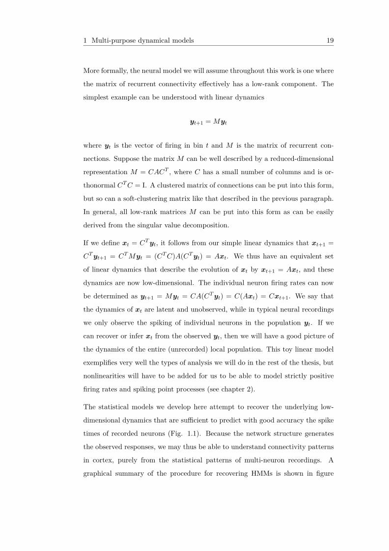
More formally, the neural model we will assume throughout this work is one where
the matrix of recurrent connectivity effectively has a low-rank component. The
simplest example can be understood with linear dynamics
yt+1 = Myt
where yt is the vector of firing in bin t and M is the matrix of recurrent con-
nections. Suppose the matrix M can be well described by a reduced-dimensional
representation M = CACT , where C has a small number of columns and is or-
thonormal CTC = I. A clustered matrix of connections can be put into this form,
but so can a soft-clustering matrix like that described in the previous paragraph.
In general, all low-rank matrices M can be put into this form as can be easily
derived from the singular value decomposition.
If we define xt = CTyt, it follows from our simple linear dynamics that xt+1 =
CTyt+1 = CTMyt = (CTC)A(CTyt) = Axt. We thus have an equivalent set
of linear dynamics that describe the evolution of xt by xt+1 = Axt, and these
dynamics are now low-dimensional. The individual neuron firing rates can now
be determined as yt+1 = Myt = CA(CTyt) = C(Axt) = Cxt+1. We say that
the dynamics of xt are latent and unobserved, while in typical neural recordings
we only observe the spiking of individual neurons in the population yt. If we
can recover or infer xt from the observed yt, then we will have a good picture of
the dynamics of the entire (unrecorded) local population. This toy linear model
exemplifies very well the types of analysis we will do in the rest of the thesis, but
nonlinearities will have to be added for us to be able to model strictly positive
firing rates and spiking point processes (see chapter 2).
The statistical models we develop here attempt to recover the underlying low-
dimensional dynamics that are sufficient to predict with good accuracy the spike
times of recorded neurons (Fig. 1.1). Because the network structure generates
the observed responses, we may thus be able to understand connectivity patterns
in cortex, purely from the statistical patterns of multi-neuron recordings. A
graphical summary of the procedure for recovering HMMs is shown in figure

1 Multi-purpose dynamical models 20
a
xtxt−1xt−2x0
yt+1ytyt−1y1
•••
•••
CCCC
AAAAunderlying dynamics
observed neural activity
b
xtxt−1xt−2x1
ytyt−1yt−2y1
stst−1st−2s1
•••
•••
CCCC
AAAA
WWWW
observed neuralactivity
underlying dynamics
external stimulusor upstream area
c
xtxt−1xt−2x1
ytyt−1yt−2y1
ztzt−1zt−2z1
•••
•••
KKKK
AAAA
gggg
observed neuralactivity
underlying dynamics
decoded behavior(hand position)
Figure 1.2: Multi-purpose dynamical models. a) Intrinsic dynamics in neu-ral recordings. b) Dynamical encoding of feedforward inputs. c) Dynamicaldecoding of brain activity.

1 Multi-purpose dynamical models 21
1.2a, and will be detailed in the next chapter. In summary, we use the neural
activities up to time t to track the underlying dynamics, and use these dynamics
to predict neural firing at time t+1. Such tracking algorithms as we develop here
have a long history, going all the way back to the Kalman filter [Kalman, 1960].
In the picture provided by figure 1.1, other uses for dynamical models can be
devised. For example, we may want to study how a neural population collectively
encodes an external stimulus, that arrives as inputs to each neuron in the network.
In such a situation, the reduced-dimensional dynamics can still help, because
the network contribution to each neuron’s response will still be low-dimensional
following the low dimensional structure. If the recurrent contribution dominates
the feedforward inputs, then neurons in the network will essentially still respond
as weighted combinations of the stimulus-driven underlying dynamics, such as
described in the graph of figure 1.2b. The parameters of such a transformation
can still be recovered directly from data, provided we have access to the stimulus.
We describe the feedforward model in the simple linear toy model presented above.
Suppose now the dynamical evolution of the neural activities proceeds as
yt+1 = Myt + Tst
where st is the vector of external stimuli and T is a projection matrix from the
stimuli to the neurons. Following a similar derivation as before, the activities of
the low-rank dynamics xt now proceeds as
xt+1 = Axt + (CTT )st
and we can rewrite yt+1 = Cxt+1 + ((Id − CCT )T )st, where Id is the identity
matrix. So we see the activity of each neuron can still be represented in terms
of the low-dimensional stimulus-driven network activity, together with a purely
feedforward component. Depending on the modelling scenario, we will either ig-
nore the feedforward component (we assume it is small compared to the recurrent
drive, see chapter 4) or model it explicitly (chapter 5).

1 Multi-purpose dynamical models 22
Finally, a third use for dynamical models is in decoding information from multi-
unit recordings. In motor cortex, the population activity of neurons drives mus-
cles and produces movements. Thus, a relationship exists between neural activity
and movements, which we may be able to capture by driving a dynamical system
with inputs from the recorded neural activity (Figure 1.2c). Good performance
in capturing such transformations may eventually enable good brain machine
interfaces of the kind useful in medical prosthetic applications.
Using the toy linear model we have used above, we assume that kinematic vari-
ables zt (position, velocity etc.) are driven linearly by the network state such
that zt = Qxt, a direct projection from the latent dynamics xt. Thus we get the
picture presented in figure 1.2c, where we use the recorded neural activity yt to
estimate xt, and in turn use xt to estimate the kinematic variables zt. Again we
emphasize that the toy linear model is a simplification and nonlinearities need
to be added to this simplified picture. For the decoder, a nonlinearity g was
necessary to transform signals from the latent space to the physical space of the
kinematic variables.
Examples of each of these three uses of our dynamical systems framework can
be found throughout this work. Chapters 2, 3 and 5 use the intrinsic dynamics
recovery model (Fig. 1.2a), chapters 4 and 5 use the stimulus-driven models of
dynamics (Fig. 1.2b), and chapter 3 also uses the dynamical decoder of neural
activity (Fig. 1.2c).

II
Recurrent linear models of
simultaneously-recorded
neural populations
OutlinePopulation recordings of neurons with a temporal structure that occurs onlong timescales are often best understood in terms of a shared underlying low-dimensional dynamical process. Advances in recording technology provide accessto an ever larger fraction of the neural population, but the standard compu-tational approaches available to identify the collective dynamics scale poorlywith the increasing sizes of these datasets. Here we describe a new, scalableapproach to discovering the low-dimensional dynamics that underlie simultane-ously recorded spike trains from neural populations. Our method is based onrecurrent linear models (RLMs) and relates closely to timeseries models basedon recurrent neural networks. We formulate RLMs for neural data by general-ising the Kalman-filter-based likelihood calculation for latent linear dynamicalsystems (LDS) models to incorporate a generalised-linear observation process.We show that RLMs describe motor-cortical population data better than eitherdirectly-coupled generalised-linear models or latent linear dynamical system mod-els with generalised-linear observations. We also introduce the cascaded linearmodel (CLM) to capture low-dimensional instantaneous correlations in neuralpopulations. The CLM describes the cortical recordings better than either Isingor Gaussian models and, like the RLM, can be fit exactly and quickly. The CLMcan also be seen as a generalization of a low-rank Gaussian model, in this casefactor analysis. The computational tractability of the RLM and CLM allow bothto scale to very high-dimensional neural data.

2 Introduction 24
2.1 Introduction
1 Many essential neural computations are implemented by large popula-
tions of neurons working in concert, and recent studies have sought both
to monitor increasingly large groups of neurons [Schneidman et al., 2005,
Buzsaki, 2004] and to characterise their collective behaviour [Pillow et al., 2008,
Churchland et al., 2007]. Here we introduce a new computational tool to model
coordinated behaviour in very large neural data sets. While we explicitly con-
sider only multi-electrode array recordings of spiking neurons, the same model
can be readily used to characterise data generated by the two-photon imaging of
population activity using calcium-sensitive indicators, EEG, fMRI or even large
scale biologically-faithful simulations.
The activity of neural populations may be represented at each time point by a vec-
tor yt with as many dimensions as neurons, and as many indices t as time points
in the experiment. For spiking neurons, yt will have positive integer elements cor-
responding to the number of spikes fired by each neuron in the time interval corre-
sponding to the t-th bin. As others before [Yu et al., 2006, Macke et al., 2011], we
assume that the coordinated activity reflected in the measurement yt arises from
a low-dimensional set of processes, collected into a vector xt, which is not directly
observed. However, unlike previous studies, we construct a recurrent model in
which the hidden processes xt are driven directly and explicitly by the measured
neural signals y1 . . .yt−1. This assumption simplifies the estimation process: we
assume for simplicity that xt evolves with linear dynamics, and affects the fu-
ture state of the neural signal yt in a generalised-linear manner, although both
assumptions may be relaxed. As in the latent LDS, the resulting model enforces
a “bottleneck”, whereby predictions of yt based on y1 . . .yt−1 must be carried by
the low-dimensional xt.
State prediction in the RLM is related to the Kalman filter [Kalman, 1960] and
we show in the next section a formal equivalence between the likelihoods of the1The data used in this chapter has been generously made available by Krishna Shenoy and
was recorded in his laboratory by Mark Churchland.

2 From Kalman filters to recurrent linear models 25
RLM and a latent LDS model when observation noise is normally distributed.
However, spiking data is not well modelled as Gaussian, and the generalisation of
our approach to Poisson noise leads to a departure from the latent LDS approach.
Unlike LDS models with conditionally Poisson observations, the parameters of our
model can be estimated efficiently and without approximation. We show that,
perhaps in consequence, the RLM can provide superior descriptions of neural
population data.
2.2 From Kalman filters to recurrent linear mod-
els
Consider a latent LDS model with linear-Gaussian observations (which we will
abbreviate as GLDS). Its graphical model is shown in Fig. 2.1 (top). The latent
dynamics are parametrised by a dynamics matrix A and innovations covariance
Q that describe the evolution of the latent state xt:
P (xt|xt−1) = N (xt|Axt−1, Q) ,
where N (x|µ,Σ) represents a normal distribution on x with mean µ and
(co)variance Σ. For brevity, we omit here and below the special case of the
first time-step, in which x1 is drawn from a multivariate Gaussian. The output
distribution involves an observation loading matrix C and a noise covariance R
often taken to be diagonal so that all covariance is modelled by the latent process:
P (yt|xt) = N (yt|Cxt, R) .
In this GLDS, the joint likelihood of the observations {yt} can be written as the
product:
P (y1 . . .yT ) = P (y1)T∏t=2
P (yt|y1 . . .yt−1)
and can be computed using the usual Kalman filter approach to find the condi-
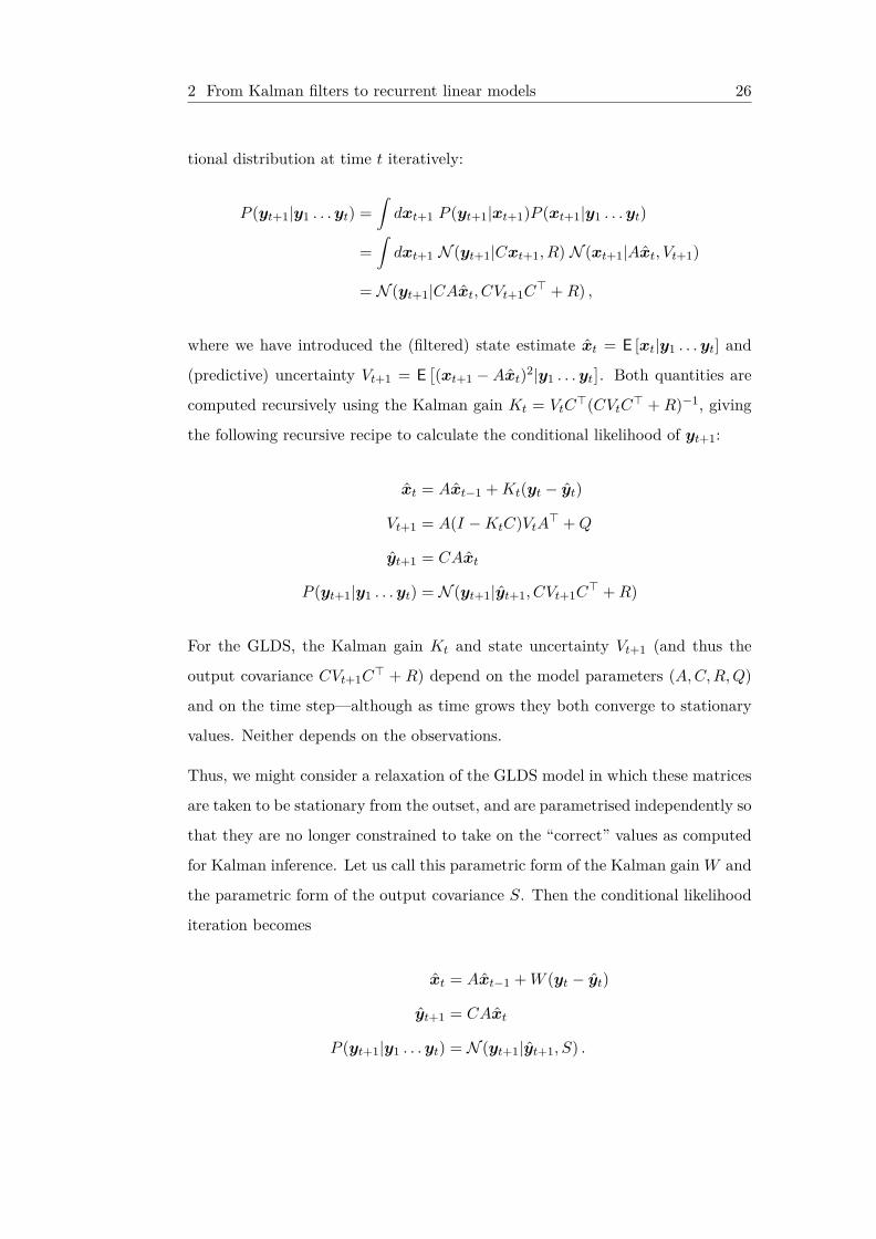
2 From Kalman filters to recurrent linear models 26
tional distribution at time t iteratively:
P (yt+1|y1 . . .yt) =∫dxt+1 P (yt+1|xt+1)P (xt+1|y1 . . .yt)
=∫dxt+1 N (yt+1|Cxt+1, R) N (xt+1|Axt, Vt+1)
= N (yt+1|CAxt, CVt+1C> +R) ,
where we have introduced the (filtered) state estimate xt = E [xt|y1 . . .yt] and
(predictive) uncertainty Vt+1 = E[(xt+1 −Axt)2|y1 . . .yt
]. Both quantities are
computed recursively using the Kalman gain Kt = VtC>(CVtC> + R)−1, giving
the following recursive recipe to calculate the conditional likelihood of yt+1:
xt = Axt−1 +Kt(yt − yt)
Vt+1 = A(I −KtC)VtA> +Q
yt+1 = CAxt
P (yt+1|y1 . . .yt) = N (yt+1|yt+1, CVt+1C> +R)
For the GLDS, the Kalman gain Kt and state uncertainty Vt+1 (and thus the
output covariance CVt+1C> + R) depend on the model parameters (A,C,R,Q)
and on the time step—although as time grows they both converge to stationary
values. Neither depends on the observations.
Thus, we might consider a relaxation of the GLDS model in which these matrices
are taken to be stationary from the outset, and are parametrised independently so
that they are no longer constrained to take on the “correct” values as computed
for Kalman inference. Let us call this parametric form of the Kalman gain W and
the parametric form of the output covariance S. Then the conditional likelihood
iteration becomes
xt = Axt−1 +W (yt − yt)
yt+1 = CAxt
P (yt+1|y1 . . .yt) = N (yt+1|yt+1, S) .

2 From Kalman filters to recurrent linear models 27
Figure 2.1: Graphical model representations of linear dynamical systems (top,middle) and recurrent linear models (bottom). Shaded variables are observed,non-shaded circles are latent random variables and squares are variables thatdepend deterministically on their parents. The middle graph redraws the LDSin terms of the innovations ηt = xt − Axt−1 to facilitate the transition towardsthe RLM. The RLM model is then obtained by replacing ηt (middle) with adeterministic prediction W (yt − yt).
The parameters of this new model are A,C,W and S. This is a relaxation of
the latent GLDS model because W has more degrees of freedom than Q, as does
S than R (at least if R is constrained to be diagonal). The new model has a
recurrent linear structure in that the random observation yt is fed back linearly
to perturb the otherwise deterministic evolution of the state xt. We call it a
Gaussian Recurrent Linear Model (GRLM).
A graphical representation of this model is shown in Fig. 2.1 (bottom), along
with a redrawn graph of the LDS model (middle). The RLM can be viewed as
replacing the random innovation variables ηt = xt − Axt−1 with data-derived
estimates W (yt − yt); estimates which are made possible by the fact that ηtcontributes to the variability of yt around yt.

2 Recurrent linear models with Poisson observations 28
2.3 Recurrent linear models with Poisson observa-
tions
The discussion above has transformed a stochastic latent LDS model with Gaus-
sian output to an RLM with deterministic latent, but still with Gaussian output.
Our goal, however, is to fit a model with an output distribution more suitable
for modelling the binned point-processes that characterise neural spiking. Both
linear Kalman-filtering steps above and the eventual stationarity of the infer-
ence parameters depend on the joint Gaussian structure of the GLDS model.
They would not apply if we were to begin a similar derivation from an LDS
with Poisson output. However, a tractable approach to modelling point-process
data with low-dimensional temporal structure may be provided by introducing a
generalised-linear output stage directly to the RLM (a model we call a gl-RLM).
This model is given by:
xt = Axt−1 +W (yt − yt)
g(yt+1) = CAxt (2.1)
P (yt+1|y1 . . .yt) = ExpFam(yt+1|yt+1)
where ExpFam is an exponential-family distribution such as Poisson, and the
element-wise link function g allows for a nonlinear mapping from xt to the pre-
dicted mean yt+1. In the following, we will write f for the inverse-link as is more
common for neural models, so that yt+1 = f(CAxt).
The simplest Poisson-based gl-RLM might take as its output distribution
P (yt|yt) =∏i
Poisson(yti|yti); yt = f(CAxt−1)) ,
where yti is the spike count of the ith cell in bin t and the (inverse) link f is
non-negative. However, comparison with the output distribution derived for the
GRLM suggests that this choice would fail to capture the instantaneous covari-
ance that the LDS formulation transfers to the output distribution (and which

2 Recurrent linear models with Poisson observations 29
appears in the low-rank structure of S above). We can address this concern in two
ways. One option is to bin the data more finely, thus diminishing the influence
of the instantaneous covariance. The alternative is to replace the independent
Poissons with a correlated output distribution on spike counts. The cascaded
generalized-linear model introduced below is a natural choice, and we show that
it captures instantaneous correlations faithfully with very few hidden dimensions.
In practice, we also sometimes add a fixed input µt to equation 2.1 that varies in
time and determines the average behavior of the population or the peri-stimulus
time histogram (PSTH).
yt+1 = f (µt + CAxt)
Note that the matrices A and C retain their interpretation from the LDS mod-
els. The matrix A controls the evolution of the dynamical process xt. The
phenomenology of its dynamics is determined by the complex eigenvalues of A.
Eigenvalues with moduli close to 1 correspond to long timescales of fluctuation
around the PSTH. Eigenvalues with non-zero imaginary part correspond to os-
cillatory components. Finally, the dynamics will be stable if and only if all the
eigenvalues lie within the unit disc. The matrix C describes the dependence
of the high-dimensional neural signals on the low-dimensional latent processes
xt. In particular, equation 2.2 determines the firing rate of the neurons. This
generalized-linear stage ensures that the firing rates are positive through the link
function f, and the observation process is Poisson. For other types of data, the
generalized-linear stage might be replaced by other appropriate link functions
and output distributions.
2.3.1 Relationship to other models
RLMs are also related to recurrent neural networks (RNN) [Elman, 1990].
An RNN can be obtained from the RLM by replacing the innovation term
W (yt−1 − yt) with Wyt−1 and adding a nonlinearity in the hidden process
xt = h (Axt−1 +Wyt−1). We found that using sigmoidal or threshold-linear

2 Recurrent linear models with Poisson observations 30
functions h resulted in models as good as the linear version of the model for
the dataset used in this paper and so we restrict our attention to simple linear
dynamics. We also found that using the full prediction error term W (yt−1 − yt)
resulted in better models than the simple RNN formulation, and we attribute
this difference to the similarity of the RLM to Kalman filter models.
We might also consider a more straightforward generalization of the LDS to
generalized-linear observations, recently proposed as the Poisson-LDS model
[Macke et al., 2011], which directly replaces the Gaussian output distribution of
the LDS with a Poisson output. The main difficulty with such models is the
intractability of the estimation procedure. For an unobserved latent process xt,
an inference procedure needs to be devised to estimate the posterior distribution
on the entire sequence x1 . . .xt. For linear-Gaussian observations, this inference
procedure is tractable and corresponds to the Kalman smoother. However, with
generalized-linear observations the inference becomes intractable and approxima-
tions need to be devised like those of [Macke et al., 2011]. These approximations
are computationally intense and can jeopardize the quality of the fitted models.
In contrast, in our model xt is a deterministic function of the data. In other
words, the Kalman filter has been built into the model as the accurate estima-
tion procedure and fitting the model can be done efficiently by standard gradient
ascent on the log-likelihood of the model. Empirically we did not encounter local
minima issues during optimization, as reported for LDS type models fitted with
an EM algorithm [Buesing et al., 2012]. Multiple restarts from different random
values of the parameters always led to models with similar likelihoods.
Notice that in order to estimate the matrices A and W the gradient needs to
be backpropagated through successive iterations of equation 2.1. This technique
is known as backpropagation-through-time (BPTT) and has been initially de-
scribed by [Rumelhart et al., 1986] as a technique to fit recurrent neural network
models. More recent implementations have proved to be state-of-the-art language
models [Mikolov et al., 2011]. BPTT is thought to be inherently unstable when
propagated past many timesteps and often the gradient is truncated after several
time steps [Mikolov et al., 2011]. We found that using large values of momentum

2 Cascaded linear models 31
in the gradient ascent alleviates these instabilities and allowed us to use BPTT
without the truncation.
2.4 Cascaded linear models
Our derivation of RLMs from LDS models has motivated us to search for similar
extensions of Gaussian models to describe correlated distributions on simulta-
neous spike counts. Such distributions are useful in modelling neural activity
when we ignore the temporal structure of the dynamics. We can instead de-
scribe solely the distribution of spike counts y recorded during brief temporal
windows [Schneidman et al., 2005] (note that we have dropped the time index
t). By describing the distribution of y we can determine what parts of the large
N -dimensional space are visited by the neural activity. What types of models
should we use to describe the distribution of y? The simplest perhaps is a Gaus-
sian model which can accurately capture the full covariance structure of y. The
weakness of the Gaussian model is that it assumes continuous-valued vectors y,
which spike counts obviously are not.
As with the derivation of the RLM from the Kalman filter, we obtain a new
generalization of a Gaussian model to spike count data. The distribution of a
multivariate variable y can be factorized as a product of multiple one-dimensional
distributions:
P (y) =N∏n=1
P (yn|y<n) . (2.2)
Here n indexes the neurons up to the last neuron N . For a Gaussian distributed
y, the conditionals P (yn|y<n) are linear-Gaussian but we can change these one-
dimensional distributions to generalized-linear observations just like we did for
the RLM
yn = f(µn + STn y<n
)(2.3)
P (yn|y<n) = Poisson (yn) . (2.4)

2 Cascaded linear models 32
The prediction for neuron n must be based only on the activities of the neurons
with indices up to n − 1 (written y<n). When f is linear and the Poisson con-
ditionals are replaced with Gaussians, equations 2.3 and 2.4 describe exactly all
full-covariance Gaussians. If the covariance of the Gaussian model is Σ, a simple
calculation shows that
Sn = 1(Σ−1)n,n
(Σ<n,<n)−1n,<n . (2.5)
Our goal however was to define a low-dimensional model on instantaneous spike
count data. This can be achieved for linear-Gaussian observations if instead of
starting from any full-covariance Gaussian model, we start from a factor analysis
model [Bishop, 2006]. Factor analysis assumes the data is generated from a low-
dimensional latent process x ∼ N (0, I), where I is the identity matrix. y is
then obtained such that P (y|x) = N (Λx,Ψ) with Ψ a diagonal matrix and Λ a
loading matrix. In factor analysis, the covariance of y is Ψ + ΛΛT . If we repeat
the derivation of equations 2.3, 2.4 and 2.5 for this covariance matrix, we obtain
an expression for Sn via the matrix inversion lemma:
Sn = 1(Σ−1)n,n
(Ψ<n,<n + Λ<nΛT<n
)−1
n,<n
= 1(Σ−1)n,n
(Ψ−1<n,<n + Ψ−1
<n,<nΛ<n + · · ·)n,<n
,
where the dots omit further factors in the inverse matrix expansion. Taking into
account that Ψ is diagonal, we see that Sn is a linear combination of the columns
of Ψ−1Λ for all n, followed by a truncation to the first n − 1 elements. If we
arrange all Sn as upper columns of an N by N matrix S, then we can write
S = upper(zwT
)for some low-dimensional matrices z = Ψ−1Λ and w, where the
operation upper extracts the strictly upper triangular part of a matrix. Finally,
we can easily impose this constraint on S even for generalized-linear observations.
The resulting cascaded linear model (CLM) is shown to provide better fits to
binarized neural data than standard Ising models (see the Results section), even
with as few as three dimensions of common input.

2 Alternative models 33
Another strong property of the CLM is that it allows stimulus-dependent inputs
in equation 2.3. The CLM can also be used in combination with the RLM, where
the CLM replaces the observation model of the RLM. This approach can be useful
when large bins are used to discretize spike trains. In both cases the model can
be estimated quickly with standard gradient ascent techniques.
2.5 Alternative models
2.5.1 Alternative for temporal interactions: causally-
coupled generalized linear model
One popular and simple model of simultaneously recorded neuronal populations
[Pillow et al., 2008] constructs temporal dependencies between units by directly
coupling a neuron’s probability to fire with the histories of all other neurons and
its own history as described by the following equation:
yt ∝ Poisson(f(µt +Nt∑i=1
Bi (hi ? yt)))
hi ? yt are convolutions of the spike trains with a set of basis functions hi and
Bi are the pairwise interaction terms. Each matrix Bi has N2 parameters where
N is the number of neurons, so the number of parameters grows quadratically
with the population size. This type of scaling makes the model prohibitive to
use with large-scale array recordings. Even with aggressive regularization tech-
niques, the model’s parameters are difficult to identify with limited amounts of
data. Perhaps more importantly, the model does not have a physical interpre-
tation. Neurons recorded in cortex are rarely directly connected, and retinal
ganglion cells almost never directly connect to each other. Instead, such directly
coupled GLMs are used to describe so-called functional interactions between neu-
rons [Pillow et al., 2008]. We believe a much better interpretation for the corre-
lations observed between pairs of neurons is that they are caused by common
and low-dimensional inputs to these neurons and the models we propose here,
the RLM and the CLM, are aimed at discovering these inputs.

2 Results 34
2.5.2 Alternative for instantaneous interactions: the Ising
model
For instantaneous interactions, a model from statistical physics is available that
can also capture the full covariance structure of y if we assume that each entry
in y is either 0 or 1 [Schneidman et al., 2005]. This is called the Ising model and
is given by equation
P (y) = 1Z
eyT Jy. (2.6)
where J is a pairwise interaction matrix and Z is the partition function, or the
normalization constant of the model. The model’s attractiveness is that for a
given covariance structure it makes the least assumptions about the distribution
of y, or in other words has the largest entropy. However, the Ising model and the
so-called functional interactions J have no physical interpretation when applied
to data recorded in the brain. Furthermore, Ising models are difficult to fit as
they require estimates of the gradients of the partition function Z. The models
become much more difficult to estimate with an increasing number of neurons
as the number of parameters grows quadratically with the number of neurons.
Ising models are even harder to estimate when stimulus-dependent inputs are
added in equation 2.6. For datasets collected in the retina or other sensory
areas [Schneidman et al., 2005], much of the covariability in y is expected to be
due to a common stimulus input. Another short coming of the Ising model is
that it can only model binarized data and cannot be normalized for integer y’s
[Macke et al., 2011], so either the time bins need to be reduced to ensure no
neuron fires more than one spike in a single bin or the spike counts must be
capped at 1.

2 Results 35
a
b
Figure 2.2: Experiments on simulated data. a) Shows a schematic of generat-ing pseudo-data from diverse generative models, including a ground truth PLDSmodel, ground truth RLM model and a realistic PLDS model fit to array record-ings. b) Shows the performance of the models at recovering eigenvalues of dy-namics and underlying subspaces.

2 Results 36
2.6 Results
2.6.1 Simulated data
We began by evaluating RLM models fit to simulated data where the true gen-
erative parameters were known. Two aspects of the estimated models were of
particular interest: the phenomenology of the dynamics (captured by the eigen-
values of the dynamics matrix A) and the relationship between the dynamical
subspace and measured neural activity (captured by the output matrix C). We
evaluated the agreement between the estimated and generative output matrices
by measuring the principal angles between the corresponding subspaces. These
report, in succession, the smallest angle achievable between a line in one subspace
and a line in the second subspace, once all previous such vectors of maximal agree-
ment have been projected out. Exactly aligned n-dimensional subspaces have all
n principal angles equal to 0◦. Unrelated low-dimensional subspaces embedded
in high dimensions are close to orthogonal and so have principal angles near 90◦.
We first verified the robustness of maximisation of the gl-RLM likelihood by fitting
models to data that were themselves generated by a known gl-RLM. Fig. 2.2b
shows eigenvalues from several simulated RLMs and the eigenvalues recovered
by fitting parameters to simulated data. The agreement is generally good. In
particular, the qualitative aspects of the dynamics reflected in the absolute values
and imaginary parts of the eigenvalues are well characterised. Fig. 2.2b shows
that the RLM fits also recover the subspace defined by the loading matrix C, and
do so substantially more accurately than either principal components analysis
(PCA) or GLDS models. It is important to note that the likelihoods of LDS
models with Poisson observations are difficult to optimise, and so may yield poor
results even when fit to within-class data. In practice we did not observe local
optima with the RLM or CLM.
We also asked whether the RLM could recover the dynamical properties and
latent subspace of data generated by a latent LDS model with Poisson observa-
tions (PLDS). Fig. 2.2b shows that the dynamical eigenvalues of the maximum-

2 Results 37
a
5
6
7
8
9
10
11
12
13
GLMw/o SC
GLMw/ SC
PLDS 10
LDS 10
LDS 20
RLM 10
RLM 20
RLM3+PSTH
MS
Eba
selin
e−
MS
E
baseline = PSTH (low rank)
Filtering prediction on test data
b
Ising rank=1 r=2 r=3 r=4 r=50
0.01
0.02
0.03
0.04
0.05
0.06
0.07
Lik
elih
ood
per
spik
e−
baselin
e(b
its)
Figure 2.3: a) Perfomance on test data of the models that we evaluated (higheris better). GLM type models are helped greatly by self-coupling filters (whichthe other models do not have). The best model is an RLM with three latentdimensions and with a low-rank model µ of the PSTH. Adding self-couplingfilters to this model further increases its predictive performance by 5 (not shown).b) The likelihood per spike of Ising models as well as CLM models with smallnumbers of hidden dimensions. The CLM saturates at three dimensions andperforms better than Ising models.
likelihood RLM are close to the eigenvalues of generative PLDS dynamics, whilst
Fig. 2.2b shows that the dynamical subspace is also correctly recovered. Param-
eters for these simulations were chosen randomly. We then asked whether the
quality of parameter identification extended to PLDS models with realistic pa-
rameters, by generating data from a PLDS model that had been fit to a neural
recording. As seen in figs. 2.2b the RLM fits remain accurate in this regime,
yielding better subspace estimates than either PCA or GLDS.
2.6.2 Array recorded data
In this section we show that the two proposed models, RLM and CLM, better
capture the statistical structure of spike trains than previous models. In partic-
ular, we compare the RLM to the GLM, LDS and PLDS and the CLM to the
Ising model.

2 Results 38
We used a dataset of 92 neurons recorded with a Utah array implanted in the
premotor and motor cortices of a rhesus macaque monkey performing a delayed
center-out reach task. For all comparisons below we use datasets of 108 trials in
which the monkey is making movements to the same target.
We discretized spike trains in time bins of 10ms as the GLM has too many
parameters and needs to be regularized in order to make good predictions on
held-out test data. Figure 2.3a shows only the best cross-validation result for
the GLM and the results without regularization for models with low-dimensional
parametrization. The measure of performance we show in figure 2.3a is a causal
mean squared error prediction subtracted from the error which a good model of
the PSTH makes. We obtain the PSTH model by truncating at five dimensions
an SVD decomposition of the individual trial-averaged PSTHs which have been
smoothed with a Gaussian filter of standard deviation 20ms. The number of
dimensions kept and the standard deviation of the Gaussian filter have themselves
been cross-validated to find the best performance. In other words, we are assessing
the model’s ability to predict spikes on a trial by trial basis.
As another measure of performance for the RLM, we evaluated the quality of
probabilistic samples obtained from the fully fitted model. Figure 2.5 shows
averaged noise cross-correlograms obtained from a large set of samples. Note
that the PSTHs have been subtracted out from each trial to reveal only the extra
correlation structure that is not repeatable from trial-to-trial. Even with very few
hidden dimensions, the model captures the full temporal structure of the noise
correlations very well.
Since the Ising model requires binarized data, we replace all spike counts larger
than 1 with 1. The log-likelihood of the Ising model can only be estimated
for a small number of neurons, so for comparison we only consider the 30 most
active neurons. The measure of performance reported in figure 2.3b is the extra
log-likelihood per spike compared to a model that makes constant predictions
equal to the mean firing rate of each neuron. The CLM model with only three
hidden dimensions achieves the best generalization performance and surpasses the

2 Discussion 39
an
eu
ron
in
de
x
neuron index
10 20 30
10
20
30
b
neuro
n index
neuron index
10 20 30
10
20
30 −0.05
0
0.05
0.1
0.15
Figure 2.4: Samples from cascaded linear model with 3 latent dimensionsmatch the correlation structure of the real data. a) Shows the true datapairwise correlations b) Shows pairwise correlations of samples drawn from themodel distribution after fitting to the data.
Ising model. Similar results for the performance of the CLM can be seen on the
full dataset of 92 neurons with non-binarized data, indicating that three latent
dimensions suffice to describe the full space visited by the neuronal population
on a trial-by-trial basis. Finally, figure 2.4 shows that samples drawn from a
CLM model with only three dimensions almost perfectly captures the structure
of pairwise noise correlations in the data.
2.7 Discussion
The gl-RLM model, while motivated similarly to the latent LDS model, can
be fit more efficiently and without approximation to non-Gaussian data. We
have shown that it yields superior performance on simulated data, as well as
population recordings from the motor cortex of behaving monkeys. The model
is easily extended to other output distributions (such as Bernoulli or negative
binomial), to mixed continuous and discrete data, to nonlinear outputs, and to
nonlinear dynamics. For the motor data considered here, the generalised-linear
model performed as well as more completely non-linear versions.

2 Discussion 40
−100 −50 0 50 100−0.01
0
0.01
0.02
0.03
0.04
0.05
0.06
Time lag (ms)
Cor
rela
tion
Neurons 1−23Neurons 24−46Neurons 47−69Neurons 70−92
Figure 2.5: Samples from an RLM model resemble the (shuffle-corrected) cross-correlation structure of the data. Neurons were separated into four groups orderedby their total correlation and the average cross-correlograms within each groupare shown. Continuous lines are the data and the model generated samples arein dashed lines. Although the peak at 0ms may be due to recording the sameneuron multiple times on different electrodes, we have verified that in fact mostpairs of units had such a peak and no two units had unproportionately large cross-correlation peaks, as would be expected for directly-connected neurons. Due toaveraging over many pairs of neurons and trials, the error bars on the cross-correlograms were very small and are not shown.
a
1 2 3 4 5 6 10 15 200.04
0.045
0.05
0.055
0.06
0.065
0.07
Likelihoodperspike−baseline(bits)
Number of inputs to RLM
b
1 2 3 200.85
0.9
0.95
1
Eig
en
va
lue
(a
bs)
Number of inputs to RLM
Figure 2.6: When a low-dimensional PSTH model (µ) is added to the RLM,log-likelihood saturates at a very small number of latent dimensions (three) andperforms better than RLM and LDS models without PSTH terms. Without thePSTH model, we needed to use as many as ten or twenty latent dimensions tocapture the full aspects of the data. Figure b) shows the magnitudes of theeigenvalues obtained with RLM3+PSTH. Most of the trial-by-trial variability isthus explained with timescales of 100 and 200 ms.

III
Recurrent linear analysis of
multi-neuron recordings
from motor cortex
OutlineWe find two new single-trial correlates of hand movements in the motor cortex ofprimates. First, we show that trial-by-trial fluctuations in population responsesduring the delay period follow similar dynamics as those followed during actualmovements. These fluctuations are concentrated in 100-200ms long dynamicalevents which activate the entire population. In one monkey, many of the fluc-tuations were associated with short movements that were very quickly stopped.Second, using a novel decoder of population activity, we find that one axis ofneural dynamics controls the progression of movement. The neural activity alongthis axis correlated not only with reaction times but also with the fine details ofmovements like the shape of the speed profile. Our findings were made possibleby new statistical and dynamical models of population neural activity which wedeveloped, and their associated dynamics-based decoders of hand position. Us-ing a model-derived estimate, we show that the redundant information due tocorrelated fluctuations across neurons drops by a factor of 50 to almost 0 duringmovements, indicating an almost complete lack of correlated fluctuations and ahigh degree of desynchronization in the responses. Such a desynchronized regimeof neural dynamics might help cortex generate reliable and robust motor signals.

3 Neural dynamics in motor cortex 42
3.1 Neural dynamics in motor cortex
1 In this chapter we analyze the dynamics of cortical populations recorded from
motor cortex. Utah arrays were implanted into the motor cortices (primary M11The data used in this chapter has been generously made available by Krishna Shenoy and
was recorded in his laboratory by Mark Churchland.
a b
c
−500 0 500 1000 15000
20
40
60
80
100
Time (ms)
Neuro
n index
d
−200 0 200 400 600 800 1000−40
−20
0
20
40
60
Time (ms)
Firi
ng r
ate
(Hz)
e
0 20 40 6010
−2
100
102
neuron/latent−mode number
Am
plitu
de
f
−200 0 200 400 600 800 1000−100
−50
0
50
100
Time (ms)
Am
plitu
de
Figure 3.1: (Caption next page.)

3 Neural dynamics in motor cortex 43
Figure 3.1: Example multi-neuron recording in motor cortex of pri-mates. a) Picture of the kind of Utah array implanted in motor cortex. b)Schematic of the delayed reach task to one of eight locations. c) Example arrayrecording from a single trial of the task. Vertical bars indicate target onset andgo cue onset. Rasters of 97 simultaneously-recorded neurons from a Utah-arrayimplanted in the motor cortex of a rhesus macaque. d) Mean-subtracted firingrates over 108 repetitions of the same stimulus. Stimulus-onset at time 0 is fol-lowed by the delay period of one second. e) Singular value decomposition ofPSTHs recover the principal temporal dynamics. The spectrum contains severalsingular values significantly large. The spectrum of white noise with equivalentpower is also shown. f) The six temporal projections with largest singular valuesare shown. Together these account for over 95% of the variance of the populationPSTHs.
and premotor dorsal PMd) of rhesus macaque monkeys (Fig. 3.1a). Animals
were first trained to perform a delayed center-out task on a computer screen
and became experts. Subsequent to array implantation, both neural activity
and hand position were monitored during performance of the task. The task
structure was designed to provide a number of advantages for neural recordings
(Fig. 3.1b). First, the monkey had to initiate trials itself by holding its hand
in the center of the screen and fixating on this center point. Following fixation,
a target appeared while the monkey had to continue holding and fixating for a
delay period. After this delay period, a go cue was displayed in the center and
the monkey was allowed to move its hand to the target. Neural activity from a
single trial (shown in figure 3.1c) corresponds to a target onset at time 0 and an
ensuing delay period of one second. The Go cue appeared at time 1000ms and
the monkey executed the reach with typical reaction times of ∼ 200ms. Neurons
can be seen to have strong responses around stimulus onset (0 ms) and during
movements (after 1000ms) but there is also ongoing activity during the delay
period (0-1000ms). The peri-stimulus time histogram represents the stimulus-
locked mean firing rates of neurons (Fig. 3.1d). It is already obvious from figure
3.1d that the major response features of neurons can be summarized succinctly
from the PSTHs. Neurons that respond show firing rate increases at stimulus
onset, after which they either get inhibited below their baseline, or start slowly
ramping up their firing rates until the end of the trial. Although some variability

3 Statistical models of delay-period activity extract consistent single-trialpatterns 44
exists in the dynamic shape of the stimulus-response, such PSTHs can typically
be explained with very few dynamical modes. This would have not been the
case for example if each neuron had their maximal firing rates at a different time
during the trial, or if the increases and decreases in firing rates were less smooth
in time and more temporally jagged.
We can decompose the dynamics of the PSTH using a singular value decompo-
sition (SVD). Assume the firing rates of the neurons are represented in an array
PSTH(nn, t) with nn the neuron number and t the time bin number. An SVD
decomposition simply decomposes this matrix into PSTH = USV , with S a di-
agonal matrix of real singular values, U a matrix of orthogonal subspaces and V
a matrix of orthogonal temporal trajectories. The singular values of S are sorted
in order of their absolute magnitude, hence one can plot them as in figure 3.1,
which shows that for this dataset, most of the variance in the PSTHs lies in the
top two components, with perhaps additional significant variance in the next few
components. Inspecting the timecourses of these dynamical modes in figure 3.1f
reveals that indeed they mostly capture the patterns we have already pointed out
in the previous paragraph.
This simplistic description of neural responses may be sufficient for some purposes,
but ignores most of the recorded data. Our motivation in much of the work
described here is to perform such low-dimensional analysis on single trials, and
thus capture more detailed aspects of the neural responses.
3.2 Statistical models of delay-period activity ex-
tract consistent single-trial patterns
The peristimulus time histogram (PSTH) is useful for understanding neural re-
sponses under repeatable experimental conditions. However, the PSTH loses all
single-trial information that might correlate with behavioral or perceptual vari-
ability. We would like to understand the trial-to-trial variability either as a con-
sequence of different internal states, such as attentional states in sensory cortices,

3 Statistical models of delay-period activity extract consistent single-trialpatterns 45
a
yt = multineuron vectorof spike counts at time t
xt = hidden low-dimensional stateof the system at time t
xtxt−1xt−2x1
ytyt−1yt−2y1
•••
•••
CCCC
AAAA
b
zt = hand position in two-dimensional space
xtxt−1xt−2x1
ytyt−1yt−2y1
ztzt−1zt−2z1
•••
•••
WWWW
AAAA
gggg
Figure 3.2: Model structure. a) Modelling framework for capturing trial-by-trial fluctuations in neural activity not controlled by the experimenter. Theshading of the yt nodes indicates that these are observed variables, while theunderlying sources of fluctuations xt are unobserved but we make the modellingassumption that they evolve with simple linear dynamics. This model is evaluatedusing a Kalman filter optimized for Poisson spike counts. b) Second modellingframework for capturing the dependence of hand position on spiking activity inM1. We use a decoder that incorporates low dimensional dynamics as before,but is driven exclusively by the observed data. The hand position zt dependson the hidden states through a nonlinear function g that maps into the two-dimensional space of the hand location. The nonlinearity was parametrized as aone layer neural network with rectified linear units. The model parameters arefit from pairs (yt, zt). On test data, the performance of the model is evaluatedby computing the root mean squared error between the model’s predictions andthe actual reach trajectories.
or as a direct determinant of variable behavior, such as we might expect in mo-
tor cortex, where activity drives muscles and consequently enacts action. Such
variability however is by definition not linked to the experimental conditions,
therefore averaging over trials will cancel out the variability in neural responses.
Hence, we need to analyze single-trial relationships between neural variability and
behavioral events. Single-neuron recordings do not contain sufficient information
to make single trial analysis feasible. Fortunately, large-scale recordings have
recently made it possible to monitor the activity of sufficiently many neurons
in motor cortex, that we might in principle understand the patterns of neural
covariability from the single-trial population response.
In this work we focused on understanding and interpreting a reduced-
dimensionality representation of the full array recordings (Fig. 3.2a). Our di-

3 Delay period shared fluctuations are associated with micro-movements 46
mensionality reduction techniques are motivated from multiple observations.
First, we observed that a three-dimensional model of the shared covariability was
sufficient to explain the patterns in the data. Models with higher dimensionality
over-fitted to the training data, and did not increase the likelihood of the held-out
data.
Second, concentrating all covariability into a small number of dimensions might
allow us to track the typically small number of behavioral variables represented by
motor cortex. In fact, we observed that most of the covariability in motor cortex
in the delay period of the reach task could be accounted for by a single underlying
trajectory that tracked the overall level of activation of the neural population
(Fig. 3.3e). The main trajectory clustered neural single-trial fluctuations into
events extended in time about 100 to 300ms (Fig. 3.3abc). The second and third
trajectories tracked additional details of the spatial structure of these events and
contained significant power (Fig. 3.3d). One might hypothesize that such large
single-trial events would correlate with movements, and we show in the next
section that, somewhat surprisingly, this was indeed the case in one monkey.
3.3 Delay period shared fluctuations are associ-
ated with micro-movements
Although the monkey was required to hold its hand in the center of the screen
during the delay period, the effective allowed holding area was relatively large
(Fig. 3.4d). Although typical movements required of the monkeys were about 10
cm, we found that during delay period activity the hand position shifted slightly
in very brief hand drifts less than 1mm long that we call micro-movements (Fig.
3.4ef).
The micro-movements had a very stereotyped direction of drift towards the lower
left direction for a monkey using its right hand. We found that these micro-
movements were associated with large increases in the total activity of M1 neu-
rons.
3 Fluctuations in M1 activity align with population patterns during movement47
Furthermore, the micro-movements aligned in typical duration and onset with
the events captured by our low-dimensional trajectories extracted from the array
data. The micro-movement triggered multi-unit activity (MUA) had a prominent
peak at a timelag of -30 ms (Fig. 3.4g).
We compared the population vector activated by the micro-movements to the
population vectors of neural activity during distinct phases of the reaches. We
found that the population vector activated during micromovements correlated
highly to the population vector in M1 at the end of reaches (Fig. 3.4c).
This analysis suggests that the observed neural activity in M1 during micro-
movements may either be of a sensory feedback origin, or sending a stopping
signal to the arm to maintain fixation.
3.4 Fluctuations in M1 activity align with popula-
tion patterns during movement
While we found a potential role for one of the three underlying trajectories, the
question remains what the other two trajectories might be representing. We did
a similar comparison as before with the population vectors during actual move-
ments, but this time we compared them with the subspaces of neural covariability
corresponding to the trajectories.
Like before, we found that one of the trajectories correlated strongly with the
population vector at the end of movements. The other two also correlated with
population activity during movements, but had maximal correlation at the onset
and during movements respectively (Fig. 3.4ab). Together the three trajectories
seemed to tile the temporal sequence activated during movements, suggesting
that trial-to-trial covariability during the delay period actually activates the same
subspaces of activity as those activated during movements.
This observation may be contrasted with recent reports by [Kaufman et al., 2014]
showing that the PSTHs during the delay period activity actually span subspaces
orthogonal to the movement subspaces. Note that the two observations are not

3 Stimulus and movement onset drastically reduce mutual information in M148
incompatible: the average delay-period activity might be mostly tuned to the
stimulus and/or showing an average preparatory activity.
However, responses varied significantly from trial to trial, and the PSTHs do
not include information about this coordinated activity. We showed that the
subspaces accounting for the variability on single trials do align with movement-
related subspaces. In addition, sometimes the large single-trial neural events were
associated with actual micro-movements of the arm, although many neural events
did not result in movements.
3.5 Stimulus and movement onset drastically re-
duce mutual information in M1
It has been previously reported that stimulus and movement onsets in M1 re-
duce both single neuron variability across trials as well as noise correlations
between pairs of neurons ([Churchland et al., 2010]). While the analysis of
[Churchland et al., 2010] is suggestive of pervasive effects across cortex, the mag-
nitude of the reduction has not been quantified in terms of the shared variability
between neurons.
Our model provides an estimate of the redundant or mutual information in the
population responses, as explained below, and we will use this quantity to track
the total mutual information of neurons during the timecourse of the trial. Under
the fully independent model of activity, all neurons would be spiking indepen-
dently with firing rates determined completely by their baseline firing rate and
self-coupling or refractory terms. At the other extreme, a fully-correlated model
would have all neurons spiking at precisely the same times. In practice, as it
can be seen in Fig. 3.1c, neurons tend to fire together a lot more than expected
by chance from an independent model. Neurons tend to fire together during the
brief 100-200ms events.
Given these correlations in firing, observing the activity of a subset of neurons
provides information about the activities of the other neurons. This quantity is

3 Stimulus and movement onset drastically reduce mutual information in M149
called mutual information and for high-dimensional variables it cannot be esti-
mated exactly. However, an estimate can be achieved by computing the joint
entropy of the distribution of neuron responses using a model. Since the true
mutual information (MI) computation is intractable, we use the best available
model (the RLM) to get a good lower bound. If a population of neurons is how-
ever driven by the same stimulus, then some of the mutual information between
neurons will be information about the stimulus.
In analogy to noise and signal correlations, we define the noise MI as that portion
of the mutual information between neurons that cannot be explained by time-
locked responses to the stimulus MI s = MI(x1,x2,s) - MI(x1,s) - MI(x2,s). The
noise MI cannot be tractably estimated for large populations either, but model-
based estimates can be obtained.
A lower bound of MI(x1,x2,s) can be obtained using an RLM model with driving
inputs, such that each neuron receives an additional input that is a function only
of time in the stimulus. We optimize these additional parameters to obtain our
best estimate of MI(x1, x2, s). The RLM model performs best at estimating the
noise MI, because it has the highest likelihoods on held-out data. The estimates
of the mutual information between the neurons and the stimulus/movements are
easier to compute since they can be estimated simply from smoothed PSTHs.
Tracking the noise MI over the timecourse of the trial shows that indeed stimulus
and movement onsets reduced the amount of mutual information in the popula-
tion (Fig. 3.3f), or at least our best estimate of it.
The shared covariability is reduced by a factor of 3 by stimulus onset, and by
a factor of 50 by movement onset. Indeed, neural covariability is very small
and close to 0 during the movements. This indicates all the inputs to the neu-
rons are time-locked to the movements and no fluctuations in activity exist from
other sources of input. The spatiotemporal patterns of neural responses during
movements are thus reproducible from trial to trial, and much more so than the
activity during the delay period of the task.
This is especially surprising since we do know some of the sources of neural

3 Comparison with noise correlation analysis 50
covariability in M1 during movements: on every trial, the monkey performs the
same reach with slightly different reaction times and speed profiles, which should
be reflected in the neural responses.
Indeed we find that information does exist in the M1 responses that can be used to
predict with high fidelity the trial-by-trial variations in hand trajectories (shown
in the following section). The mutual information analysis suggests that this
trial-by-trial covariability is in fact very small compared to that generated in the
delay period of the task, where co-fluctuations dominate responses.
3.6 Comparison with noise correlation analysis
One might ask why we do not use noise correlations to describe population co-
variability over-and-above the PSTH instead of the noise MI. One advantage in
using the noise MI is that it accounts for the shared mutual information between
neurons over all timescales of activity, not just the arbitrarily defined temporal
binning at which noise correlations are computed.
In addition noise correlations are always non-zero because they are estimated
from finite data, even when the true noise correlations should be 0. The model-
based noise MI can however be computed on test data not used for fitting the
model and if the true noise MI is 0, then the model-based estimate cannot be
significantly different from zero. As a note of caution, the noise MI will in general
underestimate the true mutual information, as we discussed before. By using well-
performing models we can attempt to bridge the gap between the estimate and
the true value.
A further disadvantage of using the noise correlations is that all pairs of neurons
are considered equal in the histogram. However, the low-firing neurons will have
poorly estimated noise correlations. Even if the noise correlations were estimated
perfectly, for an equal noise correlation, high-firing pairs of neurons will have
large mutual information while low-firing neurons will have a small amount of
mutual information, simply because high-firing neurons have larger information

3 The fine details of movements are encoded by motor cortex 51
capacity in their spike trains. Large amounts of mutual information will in turn
better reflect the underlying unobserved processes that correlate neurons.
3.7 The fine details of movements are encoded by
motor cortex
Although the amount of noise mutual information between neurons is small during
movements, we found that covariability in responses can be used to predict hand
position on a trial-by-trial basis.
To capture the transformation between motor cortex and hand position we trained
a decoder that accumulated information from the spikes into a hidden dynamical
system that evolved with linear dynamics (Fig. 3.2b).
The hidden dynamical system representation was then used to predict hand po-
sition within the same time step, via a nonlinear one-layer neural network. The
nonlinearity was necessary to convert the representation from a linear represen-
tation of M1 activity to the highly nonlinear mapping of space implicit in the
muscles and joints of the arm. We fit this transformation model using standard
backpropagation through time techniques.
The resulting model captured the relevant information from the M1 spikes into
its low-dimensional internal representation. Further below we study this internal
representation in order to understand what the relevant M1 information is, but
first we show that the decoder captured trial-by-trial variability in movements.
We studied the performance of the decoder on held-out data (Fig. 3.5a). The
decoder with 10 hidden states achieved an average root mean squared error of
6.5mm during movements. The decoder was able to perfectly predict the reach
direction from M1 activity. However, an error of 12mm was achieved by a decoder
that only perfectly predicted reach direction and then predicted the average path
from the training set for that reach. It follows that our decoder must be capturing
additional trial-by-trial variability over-and-above the reach direction.

3 What information from the population spiking does the decoder use? 52
To further show this point, we shuffled the held-out data such that the reach
condition remained the same but the hand trajectory was chosen from another
trial of the same reach randomly. The trained decoder only achieved 13.9mm
error on the shuffled set.
One primary determinant of root mean squared (rms) error on the test trials was
reaction time. To see if the decoder predicted features of movement beyond just
the reaction time, we shuffled the data again but aligned the randomly drawn
reach path so that its reaction time was equal to the reaction time of the trial
from which neural data was used in the decoder. The decoder only achieved
8.75mm rms error on this shuffled dataset. It follows that while reaction time is
an important factor for good decoding from M1, additional single-trial movement
features were also captured by the decoder.
Inspecting the reaches on the test set we were able to find another major contrib-
utor to movement variability, namely the speed profile of the reach (Fig. 3.5C).
Various features of the speed profiles are captured by the decoder, for example
some reaches have narrow peaks around the maximum speed of the reach and the
decoder captures these peaks, while other reaches have more flat and constant
maximum speed.
3.8 What information from the population spiking
does the decoder use?
Next we analyzed the hidden trajectories computed by the decoder in order to
understand what features of the spiking were important to drive good motor
predictions.
Although we trained a 10 dimensional decoder, we found that most of the variance
of the hidden space was concentrated in only 3 components (Fig. 3.5e). 3D
plots of this three-dimensional subspace gave us an understanding of the model’s
internal representation.
Two of these three dimensions had very long integration timescales (>1s) and

3 What information from the population spiking does the decoder use? 53
effectively accumulated information about the two-dimensional direction of the
reach (Fig. 3.5d). The two-dimensional plane also encoded significant lateral
deviations from the desired reach direction. To our knowledge, such a simple two-
dimensional representation of reach direction has not been shown before in M1.
It is especially noteworthy to mention that the same two-dimensional projection
encoded the same reach direction before and after movement onset.
To directly test the influence of neural spiking on the decoded movements, we
added perturbations in the two dimensional hidden space along two orthogonal di-
rections (Fig. 3.6ab). The perturbations biased the reaches significantly towards
the direction represented by the perturbations, but left relatively unaffected the
other details of the movements, like end point of the trajectory and the speed
profile. What then stopped the hidden trajectories from generating movements
before movement onset? In fact, the third dimension of the hidden state did not
evolve at all before movement onset, and grew monotonically after onset (Fig.
3.5e). This dimension had a much shorter timescale of 200ms, on the order of the
duration of the movement.
We hypothesized that this dimension controlled not only movement onset, but
also the overall progression of movement during reach. Faster rates of increase in
the latent trajectory would correspond to faster progression in movement space.
To test this hypothesis directly, we added small positive perturbations in the la-
tent trajectory at various times during the movement, and analyzed the resulting
direction of the perturbation in movement space (Fig. 3.6c).
Depending on the reach direction and hand position in space, positive pertur-
bations in the third trajectory always advanced the hand position towards the
correct target, resulting in a radial pattern of perturbations in movement space.
To our knowledge, this is the first evidence that motor cortex tracks the progres-
sion of movement and does so in a relatively straightforward fashion, controlled
only by the cumulative projection of M1 spiking onto a single linear subspace.
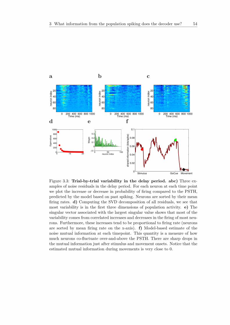
3 What information from the population spiking does the decoder use? 54
a
Time (ms)
neuro
n index
0 200 400 600 800 1000
20
40
60
80
b
Time (ms)
neuro
n index
0 200 400 600 800 1000
20
40
60
80
c
Time (ms)
neuro
n index
0 200 400 600 800 1000
20
40
60
80
d
0 10 200
200
400
600
800
1000
Eig
en
va
lue
s
e
0 50 100−0.1
0
0.1
0.2
0.3
neuron index
We
igh
t
f
Stimulus GoCue Movement0
0.02
0.04
0.06
0.08
0.1share
d info
rmation (
bits/s
pik
e)
Figure 3.3: Trial-by-trial variability in the delay period. abc) Three ex-amples of noise residuals in the delay period. For each neuron at each time pointwe plot the increase or decrease in probability of firing compared to the PSTH,predicted by the model based on past spiking. Neurons are sorted by their meanfiring rates. d) Computing the SVD decomposition of all residuals, we see thatmost variability is in the first three dimensions of population activity. e) Thesingular vector associated with the largest singular value shows that most of thevariability comes from correlated increases and decreases in the firing of most neu-rons. Furthermore, these increases tend to be proportional to firing rate (neuronsare sorted by mean firing rate on the x-axis). f) Model-based estimate of thenoise mutual information at each timepoint. This quantity is a measure of howmuch neurons co-fluctuate over-and-above the PSTH. There are sharp drops inthe mutual information just after stimulus and movement onsets. Notice that theestimated mutual information during movements is very close to 0.

3 What information from the population spiking does the decoder use? 55
a b c
d e f
1mm
g
−200 −100 0 100 2005
10
15
Time (ms)
Mea
n fir
ing
rate
(H
z)
h
Stimulus 500 10000
100
200
300
400
Time (ms)
Num
ber
of events
Figure 3.4: Movement slips in the delay period correlate with neuralevents. abc) All three dimensions of covariability in the delay period correlatewith the population vectors during movements, at different delays. Third dimen-sion of covariability correlates with the population vector during stopping at theend of the reaches. d) Subsets of movements to the eight targets. e) Zoom inof the center holding area and movements restricted to the delay period. Stereo-typical small drifts in the south-west direction are now apparent during holding.f) (X,Y) position as a function of time for several delay periods. g) AveragedMUA aligned to the micro-movements. Rise in neural activity 50ms before amicromovement could imply a causal relationship between neural activity andbehavior. h) Histogram of micro-movement times. Most micro-movements aretriggered by the stimulus. The rate of micro-movement occurrence decays duringthe delay.

3 What information from the population spiking does the decoder use? 56
arootMSE
STM[2] 21.0mmMTM[2] 11.0mmMTM[2](shuffled) 11.9mmRLM-6 6.60mmRLM-10 6.45mmRLM-30 6.55mmRLM-10(shuffled)
13.9mm
RLM-10(shuffled&aligned)
8.75mm
bmean
actual
decoded
c
200 300 400 500 200 300 400 500 200 300 400 500
200 300 400 500 200 300 400 500 200 300 400 500
200 300 400 500 200 300 400 500Time (ms)
Data
Decoded
d e
1 2 3 4 5 6 7 8 9 100
2
4
6
Spectrum of PCA
Move Onset
Move End
Figure 3.5: Single-trial decoding during reaches. a) Root mean squarederror results compared to previous state-of-the-art decoders on the same dataset,as well as results under various shuffling manipulations. b) Example decodedtrajectories on held-out data, one for each direction of movement. Note theinitial downward direction of the orange trajectory is decoded successfully. c)Examples of speed profiles of actual and decoded movements, one for each reachdirection. Note the decoder captures not only reaction time variability, but alsoother shapes of the speed profile like the peakiness/flatness of the profile. d) Topview of the three-dimensional manifold tracked by the decoder during reaches.Colors like before. e) Side view of the same manifold.

3 What information from the population spiking does the decoder use? 57
a b c
Figure 3.6: Effect of perturbations on decoder. Example perturbations atthe onset of movements, in the two-dimensional plane that controls movementdirection. a) Partial rightward perturbation. b) Upward perturbation. c, Per-turbations in the third/oblique plane of the side view. At various points duringmovement the perturbation always has the effect of advancing the decoded tra-jectory forwards. Notice this is a highly nonlinear effect enabled by the nonlineardecoding step in the one-layer neural network represented by the function g.

IV
Quiescence in neural circuits
enhances coding of
continuous sensory streams
OutlineAnimals immersed in their natural environments receive a continuous stream ofsensory inputs. In passive animals, the sensory stream is corrupted by intrinsiclarge-scale fluctuations in neuronal activity. In the presence of ongoing fluctu-ations, neural responses to isolated sounds can still be robustly-triggered, butduring continuous streaming stimulus information is lost. Here we identify andcharacterize a cortical state termed quiescent in which ongoing fluctuating ac-tivity is much reduced, while neural responses to continuously streaming stimuliare sparse, stable and high-dimensional. Putative inhibitory cells had two-foldactivity increases relative to putative pyramidal in quiescent when compared tofluctuating states. We show that models of inhibition-dominated networks of neu-rons reproduce the coding benefits of quiescent states. However, when such modelnetworks are insufficiently stabilized by negative feedback, they develop macro-scopic chaotic behavior that we show is similar to the patterns of population-widefluctuations present in fluctuating neural activity. Quiescent brain states are es-pecially well-suited to encoding the fine patterns of sounds during continuoussensory stimulation and can encode tens of thousands of auditory stimuli. Re-cent experimental evidence suggests that the inhibition-dominated coding regimewe analyze here may be employed in active and task-engaged animals.

4 Fluctuations exist and can be quenched in active states 59
4.1 Fluctuations exist and can be quenched in ac-
tive states
1 Population-wide fluctuations in neural excitability on multiple timescales
are widely documented in neural recordings ranging from intracellular record-
ings to large-scale imaging[Constantinople and Bruno, 2011, Okun et al., 2012,
Atencio and Schreiner, 2013, Beltramo et al., 2013b]. Intracellularly, fluctua-
tions resemble spontaneous transitions from resting to hyperpolarized membrane
potentials for durations of a few hundred milliseconds. In sensory areas, they
give rise to positive noise correlations which impair coding[Luczak et al., 2009,
Rothschild et al., 2010b, Sakata and Harris, 2009]. However, correlations are re-
duced when animals engage in tasks[Cohen and Maunsell, 2009, Gu et al., 2011].
Similarly reduced is the overall rate of ongoing activity in auditory cortex when
animals are performing a task using that sensory modality. Ongoing fluctuations
and overall firing rates are also reduced in auditory cortex when animals are
running or vocalizing[Schneider et al., 2014, Eliades and Wang, 2008]. Enhance-
ments of intracortical inhibition have been shown to improve coding of stimuli
in anesthetized animals[Cardin et al., 2009, Hamilton et al., 2013]. Interestingly,
it has been shown recently that awake and active states are characterized by
significantly increased inhibitory conductances, which we propose here are an ac-
tive network mechanism for quenching network excitability[Schneider et al., 2014,
Haider et al., 2013, Kimura et al., 2014].
4.1.1 Hypothesis of unstable network activity
We hypothesized that random population fluctuations are caused by unstable
recurrent network activity. The dynamics of neurons in unstable networks can
amplify small perturbations exponentially and thus cause the whole network to
activate spontaneously. Precise stimulus responses in unstable networks are not1The work described in this chapter has been done in collaboration with Nicholas Lesica,
Carsen Stringer, Jose Garcia-Lazaro and Dmitry Lyamzin. Nick, Jose an Dmitry expertlyperformed all experiments analyzed here. Carsen helped to develop and implement the networksimulations.

4 Fluctuations exist and can be quenched in active states 60
possible, because a single exponentially amplified mode of network activity domi-
nates the spatio-temporal structure of population responses. Stimulus-selectivity
of ascending thalamic fibers is thus lost because neurons tuned to the stimulus
activate many other neurons with no direct thalamic inputs.
0 0.1 0.2 0.3 0.4 0.5 0.6 0.7 0.8 0.9 10
0.2
0.4
0.6
0.8
1 Spontaneous fluctuations Quiescent state
0 500 1000
Tria
ls
isolated tones
0 500 1000
isolated tones
0 500 1000
continuous stream
0 500 1000
continuous stream
stimulus200ms
fluctuating quiescent0
2
4
6
8
10
12
mea
n fir
ing
rate
(H
z)
spontaneous
fluctuating quiescent0.5
0.6
0.7
0.8
0.9
1
mea
n de
codi
ng a
ccur
acy
tones in silenceongoing tonesongoingspeech
fluctuating quiescent0
0.05
0.1
0.15
mea
n co
rrel
atio
ns
fluctuating quiescent0
2
4
6
8
10
MU
A F
ano
Fac
tor
a b
c d e f
Figure 4.1: Quiescent states respond reliably to continuous streams ofsound. Population rasters of recordings during stimulus presentations of eitherisolated sounds or a continuous stream of speech in either (a)) spontaneouslyfluctuating states or (b)) quiescent states. c) Decoding accuracy for both statesfor different types of stimuli. d) Mean firing rates of recorded neurons in bothstates and for different stimuli and during spontaneous activity. e) Pairwisenoise correlations in stimulus responses or spontaneous correlations. f) The FanoFactor (variance divided by mean) of the multi-unit activity (MUA).
Unstable population activity can particularly hurt coding under the demands of
active ecological behavior in a continuously streaming sensory environment. Intu-
itively, errors in neural responses to stimuli can accumulate over time, especially
in areas such as auditory cortex where synaptic depression is known to signifi-
cantly affect neural responses for hundreds of milliseconds.To test our predictions
and further characterize the stability of neural network dynamics, we recorded
spiking neural activity from auditory cortex under a fluctuating brain state and a
quiescent brain state. The quiescent state was characterized by not only reduced

4 Fluctuations exist and can be quenched in active states 61
mean firing rates both in spontaneous activity and in response to sounds, but
also the complete abolishment of population-wide fluctuations during auditory
stimulus presentation.
4.1.2 Fluctuating states do not code well in ongoing stimu-
lation, but quiescent states do
Tones preceded by silence typically elicited responses from neurons in sponta-
neously fluctuating populations (Fig. 4.1a). However, responses failed to timelock
to auditory events when tones were presented in quick succession every 150ms, or
when a continuous stream of speech was played. Decoding accuracy in fluctuating
states dropped as the complexity of the sound stream increased and the mean
firing rates were also reduced (Fig. 4.1c and 4.1d). Pairwise noise correlations in
response to stimuli progressively increased from 0.02 for isolated tones to 0.07 for
streaming tones and 0.11 for ongoing speech, almost reaching the level of sponta-
neous correlations of 0.16 (Fig. 4.1e). The Fano Factor of the summed multi-unit
activity showed a similar progression, indicating a large amount of variability in
trial-to-trial evoked activity during ongoing stimulation (Fig. 4.1f). Neurons in
quiescent populations also showed robust responses to tones preceded by silence,
but in this case the spontaneous activity preceding the evoked response was also
much reduced (Fig. 4.1b,d). Quiescent states also responded reliably and re-
producibly to continuously streaming sounds (Fig. 4.1b). Coding capabilities
were much enhanced overall when compared to the fluctuating populations and
the drop in response reliability from isolated tones to continuous sounds was less
pronounced (Fig. 4.1c,e,f) .
4.1.3 Possible mechanisms underlying quiescent states
What might produce the large discrepancies in stimulus responses between the
two states? We hypothesized that the quiescent state was dominated by stabiliz-
ing negative feedback, both in the form of inhibition and short-term adaptation.
The spike shapes of electrically recorded action potentials were clearly varying in
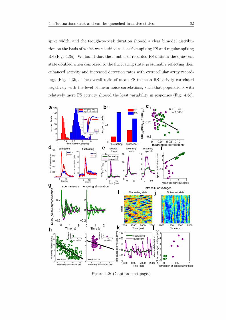
4 Fluctuations exist and can be quenched in active states 62
spike width, and the trough-to-peak duration showed a clear bimodal distribu-
tion on the basis of which we classified cells as fast-spiking FS and regular-spiking
RS (Fig. 4.3a). We found that the number of recorded FS units in the quiescent
state doubled when compared to the fluctuating state, presumably reflecting their
enhanced activity and increased detection rates with extracellular array record-
ings (Fig. 4.3b). The overall ratio of mean FS to mean RS activity correlated
negatively with the level of mean noise correlations, such that populations with
relatively more FS activity showed the least variability in responses (Fig. 4.3c).
0 0.5 10
1
2
3
4
5
correlation of consecutive trials
stan
dard
dev
iatio
nof
tria
l−av
erag
ed v
olta
ge (
mV
)
1000 1500 2000 2500−75
−70
−65
−60
−55
−50
Time (ms)
tria
l−av
erag
ed v
olta
ge (
mV
)
fluctuatingquiescent
Tria
ls
Time (ms)
Fluctuating state
Intracellular voltages
1000 1500 2000 2500Time (ms)
Quiescent state
1000 1500 2000 2500
0 0.4 0.8 1.2 1.60
20
40
60
80
100
120
time post−trough (ms)
num
ber
of c
ells
fast spiking (FS)regular spiking (RS)
−0.5 0 0.5 1 1.5 2
−0.8
−0.6
−0.4
−0.2
0
0.2
time (ms)
FSRS
0 1000
500
1000
1500
2000
2500
time (ms)
TO
TA
Lfiri
ng
rate
(Hz)
RSFS
0 1000
200
400
600
800
1000
time (ms)
TO
TA
Lfiri
ng
rate
(Hz)
RSFS
fluctuating quiescent0
0.5
1
frac
tion
of c
ells
FSRS
0 500
10
20
30
rate
FS/r
ate R
S
time (ms)
isolatedtones
fluctuatingquiescent
0 500
5
10
15
streamingtones
0 500
2
4
6
8
10
streamingspeech
0 0.04 0.08 0.12
0.5
0.75
1
mean noise correlationsra
teF
S/(
rate
FS
+ r
ate R
S) R = −0.47
p = 0.0005
0 1 2
−0.2
0
0.2
Time (s)
MU
A (
nois
e) a
utoc
orre
latio
n
spontaneous
0 1 2
−0.2
0
0.2
ongoing stimulation
Time (s)
1 3 9
0.1
1
3
0 5 10 150
5
10
15
20
25
mean firing pre−stimulus (Hz)
mea
n fir
ing
on s
timul
us (
Hz)
R = −0.76
−1 0 105
correlation
num
ber
ofda
tase
ts
0 2 40
1
2
3
4
5
6
7
mean firing pre−stimulus (Hz)
R = −0.18
−1 0 105
correlation
num
ber
ofda
tase
ts
mean spontaneous rates
spon
t rat
es a
fter
soun
d
a b c
d e f
g
h
i j
k l
quiescent fluctuating
Figure 4.2: (Caption next page.)

4 Fluctuations exist and can be quenched in active states 63
Figure 4.3: (Previous page.) Potential mechanisms for quiescent states:inhibition, adaptation and EPSP amplitude. a) Putative inhibitory cellsare classified based on their narrow spike waveforms. Spike width was measuredas the trough-to-peak duration.b) The fraction of detected FS cells was twicegreater in quiescent states. c) Ratio of FS to RS activity correlates negativelywith the mean noise correlations. d) Example tone responses in quiescent andfluctuating states. e) Ratios of firing rates between FS and RS cells at stimulus-onset are greatly amplified in quiescent states. f) Spontaneous firing rates inquiescent states are suppressed for 500ms after stimulus presentation comparedto mean rates in ongoing silence. g) Autocorrelation of the (PSTH-subtracted)MUA in (driven) and spontaneous activity. h) The firing rate in 500ms windowsbefore stimulus onset affected the magnitude of stimulus responses in fluctuatingbut not in quiescent states. ij) Intracellular voltages in quiescent and fluctuatingstates. k) Trial-averaged voltages in fluctuating and quiescent states. k) Stan-dard deviation of trial-averaged voltage plotted as a function of the similaritybetween continuous trials for 8 cells recorded in fluctuating states and 7 cellsrecorded in quiescent states.
Tones preceded by silence evoked large responses in FS and RS cells in both
quiescent and fluctuating states, but the onset of the responses showed much
larger activity in FS cells in quiescent state (Fig. 4.3d and e). The onset FS
activity appears to be optimized to activate at very short latencies, perhaps by
direct thalamic drive, and might thus serve to stabilize and sparsify the rest of
the sensory-evoked response in the local neural population.
A second source of stabilizing negative feedback that has been docu-
mented in auditory cortex is short-term adaptation[Wehr and Zador, 2005,
Destexhe et al., 2003]. We observed that firing rates in quiescent states were
suppressed relative to spontaneous rates for hundreds of milliseconds after the
stimulus was turned off (Fig. 4.3f). Similarly, the temporal autocorrelation of
the spontaneous multi-unit activity showed oscillatory activity at typical delta
band frequencies 1-2Hz but these were time-locked to the ongoing stimulation in
quiescent states (Fig. 4.3g). In fluctuating states, the level of activity preceding
a stimulus correlated negatively with the number of evoked spikes, showing that
ongoing activity can suppress the sensory response over hundreds of milliseconds
(Fig. 4.3h). The relationship did not hold in quiescent states, which had very
low levels of ongoing activity, thus insufficient to cause depression (Fig. 4.3h).

4 Deterministic network model reproduces the inherent randomness offluctuations 64
4.1.4 Intracellular voltages
We performed in vivo intracellular recordings to better understand the underlying
variability in membrane potential dynamics. We found that in both types of states
the membrane potential underwent large excursions between hyperpolarized and
depolarized levels, but in quiescent states these excursions were tightly locked to
the ongoing stimulation (Fig. 4.3i, j). The trial-averaged membrane potential
was modulated far more by the stimulus in quiescent compared to fluctuating
states and upward stimulus transients were also larger (Fig. 4.3k). The temporal
responses were similar in consecutive trials in quiescent states but quite dissimilar
during ongoing fluctuations (Fig. 4.3l).
4.2 Deterministic network model reproduces the
inherent randomness of fluctuations
We proceeded to verify in a neuronal network model that increased negative
feedback can stabilize intrinsically fluctuating activity. The architecture of the
model is described in Fig. 4.4a. Despite the wealth of studies of oscillatory
and fluctuating networks, typical models do not capture the intrinsically random
aspect of fluctuations. Even though on average population events last 200-300ms,
the duration of an event can last anywhere from 50 to 1000 ms (Fig. 4.4b).
Similarly the quiet periods between events can last for a variable interval of
time, and these durations cannot be predicted on the basis of previous neural
activity (Fig. 4.4c). To further exemplify the randomness of the fluctuations,
we found matched segments of neural activity that underwent similar patterns of
fluctuations for at least 3 seconds (Fig. 4.4f). The dynamics of these matched
segments quickly diverged after the 3 matched seconds, indicating a high-degree
of variability and potentially chaos in the timecourse of the fluctuations.
We constructed a network model with strong recurrent excitation, but relatively
weak inhibition, which reproduced the spontaneous patterns of network fluctua-
tions we observed in the data (Fig. 4.4a). The network exhibited long timescales

4 Deterministic network model reproduces the inherent randomness offluctuations 65
−100 0 1006
8
10
time fromadded spike (ms)
firin
g ra
te (H
z)
data 2
1
matched past divergent future
sim
ulat
ion
ori
gin
al+
1 sp
ike
1 s ↑added spike
feedback inhibt ion 0 200 400 600 800
100200300400500
duration (ms)
frequ
ency
302141 up state
down state
0 200 400 600 800
50
100
150
200
250
duration (ms)
frequ
ency
314203
up state
down state
200 400 600 800
100
200
300
400
500
next
dow
n st
ate
dura
tion
(ms)
up state duration (ms)
R = 0.14
200 400 600
100
200
300
next
dow
n st
ate
dura
tion
(ms)
up state duration (ms)
R = 0.13
0.02
0.04
0.06
0.08
fluctuating quiescent
tones in silence
ongoing speech
sim
ulat
ion
data
frequ
ency
stimulus
Spontaneous fluctuations Quiescent state
a b c
d e
f
g
h i
j k l
membrane potentialexcitatory currentinhibitory currentadaptation current
↑added spike500 ms
mea
n co
rrel
atio
ns
Figure 4.4: Increased inhibition reproduces transition from fluctuatingto quiescent states in network simulation. a) Schematic of network archi-tecture used throughout. b) Example distribution of up vs down state durationsmeasured from the multi-unit activity. c) Down state duration plotted as a func-tion of previous up state duration. de), Same as (bc)) but for data simulatedfrom the model. f) Two example periods of spontaneous activity matched forthe first two seconds of the rasters. g) Adding a single spike during a simulationcompletely changes the future behavior of the network. h) Example simulationof the membrane voltage with added spike. i) Trial-averaged firing rates of neu-rons in the network after adding one spike to ongoing spontaneous fluctuations.jk) Population rasters for fluctuating and quiescent simulations in response tostimulus inputs. l) Noise correlations in simulations with isolated and streamingsounds.
of fluctuations, owing to adaptation currents in single neurons, but importantly
these fluctuations came at random intervals, despite the lack of external sources of
variability (Fig. 4.4d,e). In other words, the network produced its own variability
through deterministic chaotic behavior, and such a behavior was unavoidable in
networks with weak feedback inhibition. A single spike added randomly during
ongoing spontaneous activity almost always changed the time course of the fluc-
tuations, in some cases triggering population-wide events (Fig. 4.4g). Replicating
a recent in vivo experiment[London et al., 2010], a single inserted spike was am-
plified into many more network spikes before the recurrent activity was shut off
(Fig. 4.4i). Responses to stimuli were not reliable across repeated presentations,

4 Quiescence enables sharp tuning, high-dimensional stimulus response andtemporal integration 66
but were more reliable when stimuli were presented after prolonged silence (Fig.
4.4j,l).
4.2.1 Inhibition stabilizes network activity
We were able to stabilize the fluctuations in network activity by increasing in-
hibitory feedback, such that the spontaneous activity was much reduced but
stimulus-driven activity was time-locked to the auditory stream and exhibited
near-zero trial-to-trial noise correlations (Fig. 4.4k). We could stabilize the net-
work either by increasing the inhibitory feedback gain or by adding tonic inputs
to inhibitory neurons. The network responded with equal reliability to isolated
sounds and to ongoing continuous streams of inputs (Fig. 4.4l). Adding a single
spike during evoked activity did not cause an outburst of spikes in the rest of
the network, but instead slightly inhibited network activity. Adding sufficiently
many spikes eventually shut down activity briefly due to the strong non-selective
feedback inhibition.
4.3 Quiescence enables sharp tuning, high-
dimensional stimulus response and temporal
integration
Tuning curves to sound frequency in quiescent states had on average half the
width of the tuning curves in fluctuating states and these were reproduced in
our network simulations of the two states (Fig. 4.5a). The more precisely tuned
neural responses in quiescent states enabled high decoding accuracy in a decoding
task with 29,040 different stimuli, where we pooled the responses of all neurons
recorded in quiescent states (Fig. 4.5b). To achieve good decoding accuracy
in this task at least 10-20 neural dimensions of activity were needed, indicat-
ing that the high-dimensional population activity can encode high-dimensional
stimuli (Fig. 4.5c).

4 Quiescence enables sharp tuning, high-dimensional stimulus response andtemporal integration 67
inferior colliculus auditory cortex
RLM
0 20 40 60 8010
−10
10−5
component
varia
nce
of c
ompo
nent
(pe
r ne
uron
)
multiple dimensions of variabilityin desync
0 5 10
10−4
10−3
10−2
component
varia
nce
of c
ompo
nent
(pe
r ne
uron
)
top comps have several times more variancein desync than sync
desyncsync
2 10000 29040
0
0.2
0.4
0.6
0.8
1
deco
ding
acc
urac
y
number of different stimuli
quiescentfluctuatingchance
1 128 490
0
0.2
0.4
0.6
0.8
1
deco
ding
acc
urac
y(2
9040
stim
uli)
16 dimensions
# of dimensions retained−2 −1 0 1 2
0
0.5
1
octaves
norm
aliz
ed r
espo
nse
data
−2 −1 0 1 20
0.5
1
octaves
simulation
fluctuatingquiescent
2050 2150 22500
0.5
1
1.5
2
Time (ms)
mea
n fir
ing
rate
(no
rmal
ized
)
ICA1
0 100 200
0
0.2
0.4
0.6
auto
corr
elat
ion
of m
ean
firin
g ra
te
Time(ms)
a b c
de
f g h
0 10 20 30 400.1
0.2
0.3
0.4
0.5
0.6
dimensionality of model
varia
nce
expl
aine
d of
PS
TH
fluctuatingquiescent
Figure 4.5: Quiescent states enable network to use high dimensions forcoding. a) Aligned and population-averaged tuning curves to sound frequencyin data and simulations. b) Decoding accuracy of up to 29040 stimuli. Trainingstimuli were selected as continuous 250ms long periods during a long ongoingspeech stimulus. Test stimuli were selected from a second repetition of the speechstimulus. c) Decoding accuracy with 29040 stimuli as a function of dimensionsof population responses retained. d) Schematic of a statistical model capturingthe transformation of subcortical spiking inputs into cortical spikes. e) Percentvariance explained of the PSTH by RLM transformation in a test dataset. f)Absolute variance captured by identified components of RLM transformation.g) PSTH of MUA of the inferior colliculus and auditory cortex in response tosounds without temporal structure. h) Autocorrelation of MUA in response to180 seconds of ongoing sounds without temporal structure.
We related evoked cortical responses to long segments of ongoing speech to evoked
responses to the same stimulus in the subcortical auditory pathway in the inferior
colliculus. We used a statistical modelling approach which can fit dynamical mod-
els directly to data (Fig. 4.5d). We assumed the feedforward projection from the
level of IC and through thalamus becomes input to a set of reduced-dimensionality
neural network dynamics in cortex, from which the recorded cortical neurons are

4 Conclusion 68
sampled sparsely. This model was fit directly to the data using the statistical
framework we developed in the previous chapters (the recurrent linear model,
RLM). The RLM accounted for more variance of the responses compared to a di-
rect feedforward model, and also accounted for more variance compared to a more
classical spectrotemporal model based on the frequency content of the stimulus.
In fluctuating network states, an RLM with a single underlying dynamical mode
performed almost as well as the best RLM we could train on that dataset (Fig.
4.5e). In contrast it took up to 10-20 dimensions to maximize the performance of
the model in predicting the activities of neurons in quiescent states, and the single
top dynamical mode explained only about a third of all the explained variance.
This shows that sensory-driven responses in fluctuating states are largely one-
dimensional, while a higher-dimensional response can be encoded by quiescent
states. The absolute variance of the responses predicted from subcortical inputs
was three times higher in quiescent states compared to fluctuating, and dropped
off more slowly with dimension (Fig. 4.5f).
We observed that statistical models with recurrent dynamics were able to take
advantage of their long timescales to better predict neural activity, which suggests
that cortical dynamics are integrating and transforming inputs over hundreds of
milliseconds. To test this hypothesis directly, we presented stimuli which, un-
like speech, had very short autocorrelation timescales. In every 10ms interval a
different randomly chosen frequency-modulated sweep was presented . Subcorti-
cal responses in the IC followed these sweeps faithfully, modulating their firing
rates on the same timescales as the stimulus, but cortical responses in quiescent
states were more sluggish, and instead integrated the stimuli with an autocorre-
lation timescale of 100ms followed by a negative autocorrelation at long delays,
presumably from short-term adaptation (Fig. 4.5g,h).
4.4 Conclusion
Our analysis suggests quiescent states are ideally suited to encoding sensory stim-
uli in the face of two sources of ongoing noise: the external world with its vast

4 Methods 69
amount of information bombarding the senses, and the internal world of the
brain’s own internal dynamics. Although evidence for quiescent states already
exists in active animals, more in-depth characterization of neural activity in awake
behaving animals is required to further our understanding of computations in the
engaged brain. Across brain area comparisons would also be informative. Al-
though quiescent states have been reported in auditory and barrel cortex, the
opposite has been reported in engaged visual cortex, where firing rates increase
in attentive animals. Understanding the different computational advantages of
quiescent and depolarized states might thus pave a way for understanding why
they are differentially preferred by brain areas corresponding to different senses.
4.5 Methods
4.5.1 Integrate-and-Fire Network
The results in figure 4.4 were generated through numerical simulation of a net-
work of conductance-based leaky integrate and fire neurons. There are three
currents in the model: an excitatory, an inhibitory and an adaptation current.
The subthreshold membrane potential for a single neuron i obeys the equation
τmdVidt = −(Vi − EL)− gEi(Vi − EE)− gIi(Vi − EI) +−gDi(Vi − ED).
When V > Vth, a spike is recorded in the neuron and the neuron’s voltage is
reset to Vreset = 0.9Vth. For simplicity, we set Vth = 1 and the leak voltage
EL = 0. The excitatory voltage EE = 2Vth and EI = ED = −0.5Vth. Each of
the conductances has a representative differential equation which is dependent on
the spiking of the neurons in the network at the previous time step, st−1. The
excitatory conductance obeys
τEdgEdt = −gE +Ast−1 + b.

4 Methods 70
where A is the matrix of excitatory connectivity and b is the vector of tonic inputs
to the neurons. The matrix of connectivity is all-to-all for the network of 128
neurons and their connectivities are randomly chosen from a uniform distribution
between 0 and wE . The tonic inputs b are uniformly distributed between 0 and
bmax. The inhibitory conductance obeys
τIdgIdt = −gI +
(c+
∑st−1
)p.
The adaptation conductance obeys
τEdgDdt = −gD + wDst−1.
For all the simulations in figure 2, τm = 26 ms, τE = 44 ms, τI = 39 ms, τD = 261
ms, wE = 0.15, bmax = 0.025, and p = 1.25. For the spontaneous fluctuations
simulations (parts d, e, g, h, i, j and l), wD = 0.09, wI = 0.047, c = 0. For the
quiescent simulations shown in part k and l, wD = 0.1, wI = 0.07, and c = 0.02.
Part a shows example currents from a spontaneous fluctuation simulations. Parts
d and e were produced from 8 minute simulations of the spontaneous fluctuations
state not driven by stimulus. For parts g, h, and i, single spikes were inserted
into the spontaneous fluctuations state. Part h is the membrane potential trace
for the neuron in part g which has an added spike. Part i is the average firing
rate of the network in 256 trials of 3 seconds each with a spike added in the
middle. Parts j and k are driven by a stimulus of magnitude 0.06 distributed
across 3 frequencies at a given time out of 20 possible frequencies. The tuning
of the input to each cell has a standard deviation of 4 frequencies. The tones in
silence are 100 ms long and separated by 1 s. The tones in silence were used to
compute the tuning curves in figure 4 part a.

V
Recurrent linear analysis of
state-dependent A1
population activity
OutlineIn this section we further investigate the dynamical properties of neural responsesin different brain states. We make a finer distinction between different typesof multi-neuron patterns and reproduce them in network simulations. We useour statistical modelling framework to directly characterize dynamics in anes-thetized recordings, awake-passive recordings as well as network simulations ofthese recordings. We introduce a reduced population model with four variablescorresponding to excitation, inhibition, adaptation and facilitation and use it toshow that changes in inhibitory strength can drive state-transitions in the system.

5 Cortical states 72
5.1 Cortical states
1 Cortical state varied throughout the experiments and substantially affected the
multi-neuron patterns recorded. Although typically distinguished into synchro-
nized and desynchronized, we found there was a more fine distinction between
different types of synchronized and desynchronized states. The state we referred
to as fluctuating in the previous chapter would typically subsume most synchro-
nized states, but the state we referred to as quiescent is only a particular subtype
of the desynchronized states. In the previous chapter we referred to states as
fluctuating and quiescent in order to refer directly to their phenomenology, but
in this chapter and the next we situate cortical states into the existing literature
and thus refer to states as different types of synchronized and desynchronized.
We recorded neural activity under a few different anesthetics and observed at
least four qualitatively different patterns of multi-neuron responses. A single
anesthetic typically only induced one or two different states.
The desynchronized depolarized state is characterized by an ongoing high spon-
taneous firing rate without fluctuations (Fig. 5.1a). Stimulus responses occur
reliably on every presentation. Such states have been described in Urethane anes-
thetized, sleeping and passive animals and modelled by Renart et al as a classical
balanced excitatory-inhibitory network ([Renart et al., 2010]). With appropriate
choices of parameters, such networks can cancel out correlations in inputs, at
the expense of introducing chaotic behavior and responding more to the onsets
and offsets of stimuli. The more tame version of balanced network originally
described by van Vreeswijk and Sompolinsky, has a slightly different computa-
tional role and faithfully tracks inputs instead of responding only at onsets and
offsets ([van Vreewijk and Sompolinsky, 1996]). Later on we will show that our
data favors the second version. In addition, recent results in subcortical areas
suggest there are no correlations in inputs to be cancelled out by a balanced1The work described in this chapter has been done in collaboration with Nicholas Lesica and
Carsen Stringer. Nick expertly performed all anesthetized experiments analyzed here. Carsenhelped to develop and implement the network simulations. Awake passive data was generouslyprovided by Peter Bartho.

5 Cortical states 73
a Desynchronized depolarized (Urethane)
0 1 20
10
20
30neuro
n
b Classical UP and DOWN states (Urethane and Ketamine)
0 1 20
20
stimulus1 stimulus2
ne
uro
n
c Bumpy UP and DOWN states (Ketamine)
0 1 20
50
ne
uro
n
d Desynchronized hyperpolarized (Fentanyl)
0 1 20
20
40
ne
uro
n
Figure 5.1: Cortical state varies throughout experiments and substan-tially affects the multi-neuron patterns recorded. a) The desynchronizeddepolarized state. b) The classical UP and DOWN states. c) Bumpy UP states.d) The quiescent states.
network, so the primary motivation of Renart et al has little actual relevance
([Renart et al., 2010]).
The classical UP and DOWN states have been described as ongoing transitions
between hyperpolarized and depolarized states (Fig. 5.1b). These transitions
occur randomly and stimuli presented on DOWN states may fail to elicit a re-
sponse. They contain significant power at frequencies of 1-2Hz, owing to the slow
alternations between UP and DOWN states. Such states have been described
broadly in anesthetized animals, as well as in passive animals, though they are

5 Model performance 74
not usually distinguished from the bumpy UP states we describe next. Most
classical anesthetics based on urethane, isoflurane or ketamine induce such up
states.
Bumpy UP states are relatively short, synchronized periods of population spiking
for durations of 30-100ms (Fig. 5.1c). We observed that they tend to come
together in packets of 2 or 3, and in this particular dataset even six. They contain
significant power at theta frequencies of about 10Hz, in addition to still having
power at 1-2Hz, like classical UP/DOWN states. It is possible the up states
described by Hromadka et al, 2013 in awake animals are bumpy, because the
authors of the study describe them as short and rare ([Hromadka et al., 2013]).
We only saw these types of UP states in ketamine anesthesia.
The desynchronized quiescent states are more suppressed than the other states
in both spontaneous activity and stimulus responses (Fig. 5.1d). Like depolar-
ized states they have zero pairwise noise correlations, and significantly increased
activity in fast-spiking cells. We only saw such states in Fentanyl-based anesthe-
sia, but they might have been described in previous studies of awake and active
animals (see previous section). These states code stimuli very sparsely, efficiently
and reliably.
5.2 Model performance
We applied the model of dynamics we described in chapter 2 to the state-
dependent data to analyze the nature of the statistical patterns encountered.
Most of our data was obtained with either ketamine-based or fentanyl-based
anesthesia, so we will focus our analysis on these. Ketamine-based anesthesia
induces fluctuations in neural activity, while fentanyl-based anesthesia induces a
stable, desynchronized regime of activity.
Figure 5.2 shows the performance of the RLM at capturing the multi-neuron
patterns of spikes present in the datasets. The performance of the model varies
as a function of the number of underlying trajectories. A single dimension of

5 The phenomenology of dynamics 75
a
dataset1 2 3 5 6 70
0.2
0.4
0.6
0.8
1
1.2
1.4Sharedyinformationy(bits/spike) Desync Sync
b
1 2 3 4 5 6 8 10 20 400
0.1
0.2
RLM dimension
RLM
− G
LM
(bits/s
pik
e)
RLM vs GLM −−− all spontaneous datasets
c
dataset1 2 3 4 5 6 70
0.2
0.4
0.6
0.8
1
Sha
redy
info
rmat
iony
(bits
/spi
ke)
Desync
SyncGLMRLMydimy=y1RLMydimy=y2RLMydimy=y3RLMydimy=y4RLMydimy=y5RLMydimy=y6RLMydimy=y8RLMydimy=y10RLMydimy=y20RLMydimy=y40
d
1 2 3 4 5 6 8 10 20 400
0.1
0.2
RLM dimension
RL
M −
GL
M (
bits/s
pik
e)
RLM vs GLM −−− Ketamine with stimulus
Figure 5.2: Recurrent linear model predictive performance, comparedwith GLMs. a) Model likelihoods as a function of dimensionality of underlyingdynamics. Data was recorded in complete silence. b) Likelihood advantage ofRLM models over the popular GLM framework. cd) Same as (a),(b) for contin-uous stimulus-driven activity.
dynamics already accounts for a large portion of the shared population variability,
but the higher dimensions also contain information. We compared our framework
with the popular generalized linear models (described in section 2), and found
that the RLM offered vast improvements in prediction performance (Fig. 5.2).
5.3 The phenomenology of dynamics
In most datasets recorded, underlying dynamical trajectories were clearly orga-
nized into slow (>500ms autocorrelation) and fast trajectories (30-100ms auto-
correlation). Examples are shown in figure 5.3a. The slow trajectories controlled
the periodicity of the UP and DOWN states, while the fast trajectories controlled
fast fluctuations within UP states. The eigenvalues of the dynamics matrix in
spontaneous activity of both Fentanyl and Ketamine anesthesia were used to di-
vide trajectories into a pair of fast and a pair of slow dynamics (Fig. 5.3b). The
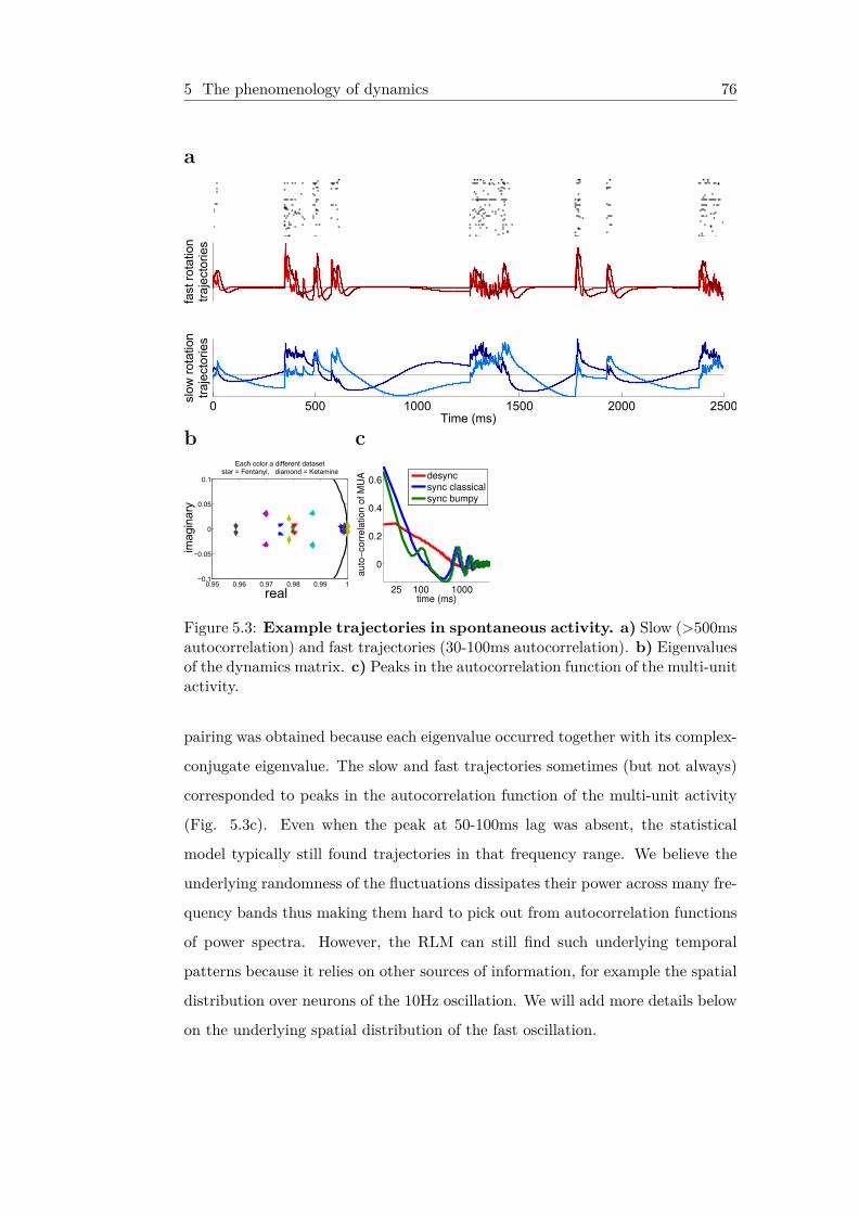
5 The phenomenology of dynamics 76
afa
st r
otat
ion
traj
ecto
ries
0 500 1000 1500 2000 2500
slow
rot
atio
ntr
ajec
torie
s
Time (ms)
b
0.95 0.96 0.97 0.98 0.99 1−0.1
−0.05
0
0.05
0.1
real
imag
inar
y
Each color a different datasetstar = Fentanyl, diamond = Ketamine
c
25 100 1000
0
0.2
0.4
0.6
time (ms)
auto
−corr
ela
tion o
f M
UA
desync
sync classical
sync bumpy
Figure 5.3: Example trajectories in spontaneous activity. a) Slow (>500msautocorrelation) and fast trajectories (30-100ms autocorrelation). b) Eigenvaluesof the dynamics matrix. c) Peaks in the autocorrelation function of the multi-unitactivity.
pairing was obtained because each eigenvalue occurred together with its complex-
conjugate eigenvalue. The slow and fast trajectories sometimes (but not always)
corresponded to peaks in the autocorrelation function of the multi-unit activity
(Fig. 5.3c). Even when the peak at 50-100ms lag was absent, the statistical
model typically still found trajectories in that frequency range. We believe the
underlying randomness of the fluctuations dissipates their power across many fre-
quency bands thus making them hard to pick out from autocorrelation functions
of power spectra. However, the RLM can still find such underlying temporal
patterns because it relies on other sources of information, for example the spatial
distribution over neurons of the 10Hz oscillation. We will add more details below
on the underlying spatial distribution of the fast oscillation.

5 The phenomenology of dynamics 77
The time-lagged cross-correlation functions between the activity of a single cell
and the summed activities of all the other cells can be organized in order of their
temporal center of mass (Fig. 5.4a). Neurons with negative (positive) centers of
mass tend to spike earlier (later) than the rest of the network. Such represen-
tations have been used to describe spike sequence patterns in hippocampus as
well as in auditory cortex. In figure 5.4 the first row shows the spike sequence
patterns for synchronized and desynchronized populations in response to a par-
ticular stimulus (a speech phone). The second row of cross-correlograms uses the
sorting derived from the first row to show the spike sequence patterns in response
to a second stimulus (a different speech phone). In synchronized states, the spikes
sequences on different phones are largely similar, while in desynchronized states
they are quite dissimilar.
The average MUA cross-correlogram latencies are similar between spontaneous
and driven activity in both states (Fig. 5.4b). Importantly, the latencies com-
puted in figure 5.4b represent the mean activities of responses to a large number
of stimuli. The specific latency changes observed in figure 5.4(a) for desynchro-
nized populations average out in figure 5.4b revealing a latency ordering much
more similar to that observed in spontaneous activity.
The model-derived trajectories capture these spike sequences in the pair of fast
complex-conjugate trajectories (Fig. 5.4c). We noticed that the fast trajectories
were out-of-phase with each other during neural responses. Neurons represented
by the first trajectory thus had an overall earlier latency on each short population
UP state. In fact, there was a continuum of phases of alignment between single
units and the trajectories, such that most neurons responded as a positively-
weighted combination of the two (Fig. 5.4d). Figure 5.4d represents each neuron’s
pair of coefficients, projected onto the unit circle, and slightly perturbed off the
circle for visualization purposes.
Latencies extracted from the cross-correlograms were well correlated with the
phases derived from the model (5.4e). Figure 5.4f shows example cross-
correlograms sorted by MUA cross-correlation latencies, while figure 5.4g shows

5 The phenomenology of dynamics 78
Figure 5.4: Spike sequences. a) The time-lagged cross-correlation between theactivity of a single cell and the summed activities of all the other cells (moredescription in the main text). b) The average MUA cross-correlogram latenciesin spontaneous and driven activity in both states. c) The model-derived trajec-tories capture spike sequences. d) Phases of alignment between single units andthe trajectories. e) Latencies extracted from the cross-correlograms were wellcorrelated with the phases computed in (d). f) Example cross-correlogram sortedby MUA cross-correlation latencies. g) The same cross-correlogram sorted by de-rived model phases.h) Explained latency variance was high for both spontaneousand average driven activity, but low for each individual phone.
the same cross-correlogram sorted by derived model phases. In desynchronized
states, the R2 value betwen latencies and model phases was high for both sponta-
neous and average driven activity, but low for each individual phone (figure 5.4f).
This suggests that although the fast trajectories describe the average responses
of the network to stimuli, each individual phone powerfully further modulates the
temporal patterns of responses with additional population dimensions of varia-
tion. This is unlike the synchronized state, where each phone’s cross-correlograms
mostly look similar.
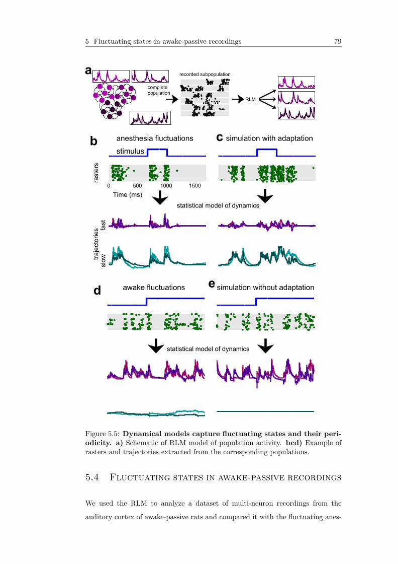
5 Fluctuating states in awake-passive recordings 79
completepopulation
RLM
recorded subpopulation
slowtrajectories
statistical model of dynamics
statistical model of dynamics
fast
0 500 1000 1500
rasters
Time (ms)
stimulus
anesthesia fluctuations simulation with adaptation
awake fluctuations simulation without adaptation
a
b c
d e
Figure 5.5: Dynamical models capture fluctuating states and their peri-odicity. a) Schematic of RLM model of population activity. bcd) Example ofrasters and trajectories extracted from the corresponding populations.
5.4 Fluctuating states in awake-passive recordings
We used the RLM to analyze a dataset of multi-neuron recordings from the
auditory cortex of awake-passive rats and compared it with the fluctuating anes-

5 Fluctuating states in awake-passive recordings 80
thetized recordings. In addition, we used the RLM to analyze spike patterns from
network simulations which we built to model the fluctuations in both anesthesia
and awake states. The RLM methodology allows us to directly validate our net-
work simulations by analyzing the underlying dynamics in both simulations and
data.
Figure 5.5a shows a simplified schematic of the RLM model of population activity,
while figures 5.5b-d show examples of rasters and trajectories extracted from four
populations: anesthesia, simulations of anesthesia patterns, awake and simula-
tions of awake patterns. Trajectories were divided into slow and fast on the basis
of their associated eigenvalues. The main difference between the anesthetized
and awake recordings was the complete absence of long timescale trajectories
in the awake data. This seems to agree with the effect of wakefulness-inducing
agents like acetylcholine, which are known to block long timescale adaptation
processes. Similarly, it was observed that adaptation processes were absent in
engaged rodents while they were learning a discrimination task, but returned
once the animals became skilled and performed the task with less engagement.
However, the fast-timescale trajectories were still present in awake states and had
similar temporal timecourses on the order of 30-50 ms. Although more analysis
is required, we postulate that these fast timescales are generated by excitatory-
inhibitory dynamics. In fact, we used this idea to generate awake-like fluctuating
states, by greatly reducing adaptation in our network simulation (see previous
section), while retaining a balance of excitation and inhibition. Note that the
awake-passive state still shows ongoing fluctuations and responds unreliably to
stimuli (not shown). Only when we also increased inhibition in the network simu-
lation were we able to stabilize the responses and get near-zero noise correlations
in stimulus responses. The state with decreased adaptation and increased in-
hibition thus resembled the urethane-anesthetized desynchronized state shown
in figure 5.1a. Further increasing inhibition put the network simulation into a
quiescent-like state, with little spontaneous activity (5.1).
To further verify our understanding of cortical states, we hypothesized that we

5 Fluctuating states in awake-passive recordings 81
a
2 4 60
5
10
15
experiment #
Fentanyl → Urethane
Sponta
neous firin
g r
ate
(H
z)
RS
FS
b Experiment 1
0
20
neuro
n
0
20
0
20
0
20
0
20
0 500 1000 1500 2000 25000
20
Time (ms)
c Experiment 2
0
20
neuro
n
0
20
0
20
0
20
0
20
0 500 1000 1500 2000 25000
20
Time (ms)
d Experiment 3
0
20
40
neuro
n
0
20
40
0
20
40
0
20
40
0
20
40
0 500 1000 1500 2000 25000
20
40
Time (ms)
e Experiment 4
0
20
40
neuro
n
0
20
40
0
20
40
0
20
40
0
20
40
0 500 1000 1500 2000 25000
20
40
Time (ms)
f Experiment 5
0
20
40
neuro
n
0
20
40
0
20
40
0
20
40
0
20
40
0 500 1000 1500 2000 25000
20
40
Time (ms)
g Experiment 6
01020
neuro
n
01020
01020
01020
01020
0 500 1000 1500 2000 25000
1020
Time (ms)
Figure 5.6: Fentanyl to Urethane transitions. a) Spontaneous firing ratesof both FS and RS cells gradually recovered during the course of several hours.b-g) Multi-neuron rasters of spontaneous activity during the entire experimentalsession.
might observe all the brain states in the same cortical population if we gradually
change the anesthetic during a long experimental session. An experiment was
started with Fentanyl anesthesia (used during surgery) and continued with Ure-
thane anesthesia. As the Urethane anesthetic started having a stronger effect and
the Fentanyl anesthetic wore off, the patterns of spontaneous multi-unit activ-

5 Four-dimensional reduced simulation of network states 82
Dnegative feedback
inhibition depression
facilitation
positive feedback
fastrecovery
recurrentexcitation
FE
I
slowrecovery
Figure 5.7: Schematic of the sources of positive and negative feedback, dividedinto fast and slow-acting mechanisms. While excitation and inhibition act andrecover quickly, facilitation and adaptation operate on longer timescales.
ity transitioned through all the cortical states described, as shown in figure 5.6.
Spontaneous firing rates of both FS and RS cells gradually recovered during the
course of the experiment (Fig. 5.6a). In the beginning of the experiment firing
was extremely sparse, but as neurons started to fire, they did so in synchronous
short bursts. As the spontaneous activity further recovered, the bursts started
coming in pairs separated by 100-200ms. For a short period of time, a state was
observed in which neurons fired regularly in short bursts that followed each other
with significant regularity about every 500ms. Eventually UP states became more
extended in time and their onsets became random and apparently chaotic. Later
on, the continuously depolarized state started replacing the fluctuating states.
5.5 Four-dimensional reduced simulation of net-
work states
To gain an intuitive understanding of the RLM trajectories and the full net-
work behavior, we constructed a four-dimensional reduced rate-based model of
dynamics. This required both slow and fast terms in the differential equations
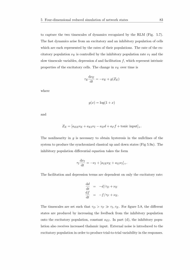
5 Four-dimensional reduced simulation of network states 83
to capture the two timescales of dynamics recognized by the RLM (Fig. 5.7).
The fast dynamics arise from an excitatory and an inhibitory population of cells
which are each represented by the rates of their populations. The rate of the ex-
citatory population νE is controlled by the inhibitory population rate νI and the
slow timescale variables, depression d and facilitation f , which represent intrinsic
properties of the excitatory cells. The change in νE over time is
τEdνEdt = −νE + g(ZE)
where
g(x) = log(1 + x)
and
ZE = [aEEνE + aEIνI − aDd+ aF f + tonic input]+.
The nonlinearity in g is necessary to obtain hysteresis in the nullclines of the
system to produce the synchronized classical up and down states (Fig 5.9a). The
inhibitory population differential equation takes the form
τIdνIdt = −νI + [aIEνE + aIIνI ]+.
The facilitation and depression terms are dependent on only the excitatory rate:
dddt = −d/τD + νE
dfdt = −f/τF + νE .
The timescales are set such that τD > τF � τI , τE . For figure 5.8, the different
states are produced by increasing the feedback from the inhibitory population
onto the excitatory population, constant aEI . In part (d), the inhibitory popu-
lation also receives increased thalamic input. External noise is introduced to the
excitatory population in order to produce trial-to-trial variability in the responses.

5 Four-dimensional reduced simulation of network states 84
The same magnitude of noise and stimulus drive the excitatory population in each
simulation.
The example nullclines in figure 5.9 explain how the system can exhibit these
diverse patterns of activity. Part (a) qualitatively describes the behavior of the
system in the synchronized classical state in the phase space of the excitatory rate
νE and the inhibitory rate νI . When the system is in a down state (not firing),
it is at the stable fixed point of the system at the origin. As the slow depression
variable recovers, the excitatory nullcline moves upwards and the unstable fixed
point of the system approaches the origin (#1). When it reaches the origin, the
system undergoes a saddle node bifurcation and the two fixed points annihilate
each other (#2), leaving only a single positive stable fixed point. The system
approaches that fixed point and remains there until the depression variable builds
up sufficiently to push the nullcline downwards (#3-4). Again, a saddle node
bifurcation occurs with the upper stable fixed point disappearing and the system
returning to the stable fixed point at the origin (#5-6).
Part (b) of figure 5.9 explains how the system can produce bumpy up states when
slightly more inhibition is introduced to the system. The slope of the excitatory
nullcline is reduced, and the excitatory and inhibitory nullclines only intersect
at a single unstable fixed point. The system oscillates around this fixed point
when the fixed point sits above zero (the trajectories are bounded in space and
thus a limit cycle exists). However, when depression increases sufficiently and
overcomes the facilitation variable, the excitatory nullcline is pushed downwards
and the limit cycle is abolished. The system then sits at the stable fixed point at
the origin until the depression variable recovers.
Figure 5.10 shows that the reduced system with external noise can reproduce
the trial-to-trial variability observed in the synchronized datasets. The model
reproduces both qualitative and quantitative features of the data.
Finally, figure 5.11 shows simulated rasters of networks with sufficient inhibitory
feedback. Responses to step inputs are reliable on each trial despite external
noise.

5 Four-dimensional reduced simulation of network states 85
on STIMULUS
off
cell
1
50
depressionfacilitation
excitationinhibition
a
b
c
d
Figure 5.8: Population dynamics simulated from the model resemble the statesobserved in the data. Access to the simulated variables allows us to understandthe phenomenology of dynamics. a-d) were obtained by successively increasingthe inhibitory feedback to the excitatory population. a) Simulation of the de-polarized desynchronized state. b) Simulation of the classical UP/DOWN statefluctuations. c, Simulation of the bumpy UP states. d) Simulation of the quies-cent network state.
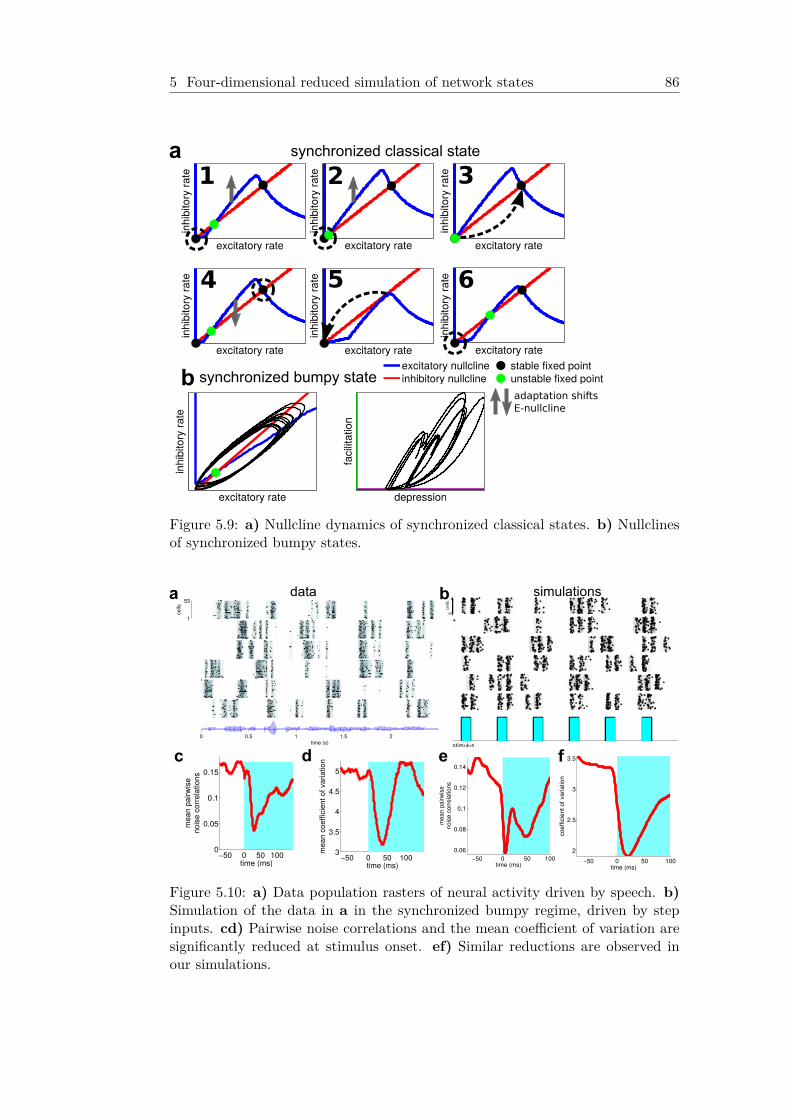
5 Four-dimensional reduced simulation of network states 86
excitatory rate
inhi
bito
ry ra
te
excitatory rate
inhi
bito
ry ra
te
excitatory rate
inhi
bito
ry ra
te
excitatory rate
inhi
bito
ry ra
te
excitatory rate
inhi
bito
ry ra
te
excitatory rate
inhi
bito
ry ra
te
1 2 3
4 5 6
excitatory rate
inhi
bito
ry ra
te
depression
faci
litat
ion
excitatory nullclineinhibitory nullcline
stable fixed point
adaptation shifts E-nullcline
unstable fixed point
synchronized classical state
synchronized bumpy state
a
b
Figure 5.9: a) Nullcline dynamics of synchronized classical states. b) Nullclinesof synchronized bumpy states.
0 0.5 1 1.5 2time (s)
1
53
cells
stimulus
cells
1
50
−50 0 50 1003
3.5
4
4.5
5
mea
n co
effic
ient
of v
aria
tion
time (ms)−50 0 50 100
0
0.05
0.1
0.15
mea
n pa
irwise
noise
cor
rela
tions
time (ms) −50 0 50 1002
2.5
3
3.5
coef
ficie
nt o
f var
iatio
n
time (ms)−50 0 50 100
0.06
0.08
0.1
0.12
0.14
mea
n pa
irwise
noise
cor
rela
tions
time (ms)
a b
c d e f
data simulations
Figure 5.10: a) Data population rasters of neural activity driven by speech. b)Simulation of the data in a in the synchronized bumpy regime, driven by stepinputs. cd) Pairwise noise correlations and the mean coefficient of variation aresignificantly reduced at stimulus onset. ef) Similar reductions are observed inour simulations.

5 Four-dimensional reduced simulation of network states 87
stimulus
cells
1
50
Figure 5.11: Population rasters of simulations of responses in the quiescent state.Noise correlations are abolished and trial-to-trial variability is low.

VI
State-dependent population
coding in primary auditory
cortex
OutlineSensory function is mediated by interactions between external stimuli and intrin-sic cortical dynamics that are evident in the modulation of evoked responses bycortical state. A number of recent studies across different modalities have demon-strated that the patterns of activity in neuronal populations can vary stronglybetween synchronized and desynchronized cortical states, i.e. in the presence orabsence of intrinsically generated up and down states. Here we investigated theimpact of cortical state on the population coding of speech in the primary audi-tory cortex (A1) of gerbils, and found that responses were qualitatively differentin synchronized and desynchronized cortical states. Activity in synchronized A1was only weakly modulated by sensory input, and the spike patterns evoked byspeech were unreliable and constrained to a small range of patterns. In contrast,responses to speech in desynchronized A1 were temporally precise and reliableacross trials, and different speech tokens evoked diverse spike patterns with ex-tremely weak noise correlations, allowing responses to be decoded with nearlyperfect accuracy. Restricting the analysis of synchronized A1 to activity withinup states yielded similar results, suggesting that up states are not equivalent tobrief periods of desynchronization. These findings demonstrate that the repre-sentational capacity of A1 depends strongly on cortical state, and suggest thatcortical state should be considered as an explicit variable in all studies of sensoryprocessing.

6 Introduction 89
6.1 Introduction
1 The representation of sensory inputs in the activity of primary cortical
areas provides the basis for higher level processing. Characterizing this
primary representation is critical for understanding sensory function, as its
nature determines the suitability of different strategies for subsequent com-
putations, and its fidelity constrains behavioral performance. The study of
sensory representations is complicated by the fact that neuronal activity is
determined not only by external inputs, but also by other sources that are
internal to the brain. In cortex, the processing of incoming stimuli can depend
strongly on brain state ([Steriade et al., 2001]; [Castro-Alamancos, 2004b];
[Haider and McCormick, 2009]; [Harris and Thiele, 2011]). In asleep, anes-
thetized, and awake animals, the state of the cortex can vary along a continuum
of synchronized and desynchronized states with different population dynamics.
When the cortex is in a synchronized state (also known as an inactivated state),
activity is characterized by slow fluctuations between intrinsically generated
up and down states, corresponding to periods of concerted spiking and silence
across large areas, and these up and down states play a major role in shaping
activity patterns ([Marguet and Harris, 2011]; [Okun et al., 2012]). Synchro-
nized states are commonly observed during slow-wave sleep and under certain
anesthetics, but recent studies have shown that the cortex can also be in a
synchronized state when animals are awake ([Crochet and Petersen, 2006];
[Greenberg et al., 2008];[Poulet and Petersen, 2008];
[Xu et al., 2012];[Luczak et al., 2013]; [Polack et al., 2013];
[Sachidhanandam et al., 2013]; [Tan et al., 2014];[Zhou et al., 2014a]).
During active sensory processing in awake animals, the cortex often tran-
sitions to a desynchronized (or activated) state in which up and down
states are suppressed and activity is strongly modulated by sensory in-
puts. Studies in the visual and somatosensory systems have observed dra-1The work described in this chapter has been done in collaboration with Nicholas Lesica.
Nick performed all experiments analyzed here. The analysis was developed jointly with Nickand Nick wrote the text.

6 Synchronized and desynchronized states in A1 90
matic differences between responses in synchronized and desynchronized states
([Castro-Alamancos, 2004a]; [Hasenstaub et al., 2007]; [Goard and Dan, 2009];
[Hirata and Castro-Alamancos, 2011]), and there are indications that such differ-
ences may also be present in A1 ([Ter-Mikaelian et al., 2007]; [Otazu et al., 2009];
[Marguet and Harris, 2011];[Guo et al., 2012];[Zhou et al., 2014a]). In this study,
we measured the activity of populations of single units in gerbil A1 in synchro-
nized and desynchronized states under different anesthetics and observed strong
effects that were evident at both the single cell and population level. We found
that cortical state modulated the selectivity, reliability, and diversity of spike
patterns, as well as the strength of noise correlations, in a manner that greatly
impacted the fidelity of the population code.
6.2 Synchronized and desynchronized states in A1
To study the impact of cortical state on the population coding of speech, we com-
pared activity recorded with a multi-tetrode array in gerbil A1 (Fig.6.1a) under
several different anesthetics. The cortical states imposed by anesthesia may, of
course, differ from those that occur naturally. However, comparisons of sponta-
neous and evoked activity in rodent A1 have revealed similar dynamical proper-
ties in the synchronized and desynchronized states observed under anesthesia and
those in awake animals ([Bermudez Contreras et al., 2013]; [Luczak et al., 2013]).
Furthermore, the use of anesthesia enabled us to control synchronization and
desynchronization without additional influences related to the particular task in
which an animal is engaged, thus allowing us to perform a general comparison of
A1 responses in the presence or absence of intrinsically generated up and down
states.
To achieve a stable and consistent synchronized or desynchronized state through-
out an entire experiment, we recorded activity under either ketamine/xylazine
(KX) or fentanyl/medetomidine/midazolam (FMM). The up and down states
that are typical of a synchronized cortical state were always evident in the pop-
ulations recorded under KX, but were largely absent in those recorded under
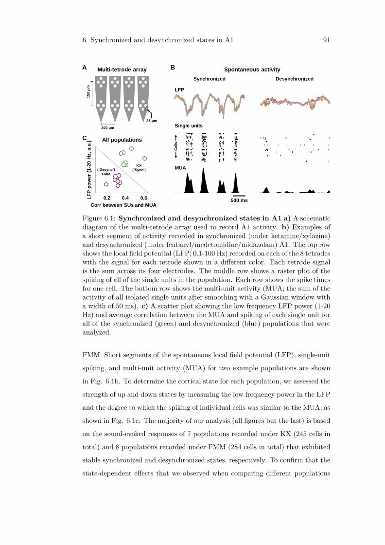
6 Synchronized and desynchronized states in A1 91
200 μm
15
0 μ
m
25 μm
Multi-tetrode array A
LFP
Single units
MUA
500 ms
Synchronized Desynchronized
All populations
(‘Desync’)
FMM
KX
(‘Sync’)
0.2 0.4 0.6 LF
P p
ow
er
(1-2
0 H
z,
a.u
.)
Corr between SUs and MUA
Spontaneous activity B
C
Ce
lls
Figure 6.1: Synchronized and desynchronized states in A1 a) A schematicdiagram of the multi-tetrode array used to record A1 activity. b) Examples ofa short segment of activity recorded in synchronized (under ketamine/xylazine)and desynchronized (under fentanyl/medetomidine/midazolam) A1. The top rowshows the local field potential (LFP; 0.1-100 Hz) recorded on each of the 8 tetrodeswith the signal for each tetrode shown in a different color. Each tetrode signalis the sum across its four electrodes. The middle row shows a raster plot of thespiking of all of the single units in the population. Each row shows the spike timesfor one cell. The bottom row shows the multi-unit activity (MUA; the sum of theactivity of all isolated single units after smoothing with a Gaussian window witha width of 50 ms). c) A scatter plot showing the low frequency LFP power (1-20Hz) and average correlation between the MUA and spiking of each single unit forall of the synchronized (green) and desynchronized (blue) populations that wereanalyzed.
FMM. Short segments of the spontaneous local field potential (LFP), single-unit
spiking, and multi-unit activity (MUA) for two example populations are shown
in Fig. 6.1b. To determine the cortical state for each population, we assessed the
strength of up and down states by measuring the low frequency power in the LFP
and the degree to which the spiking of individual cells was similar to the MUA, as
shown in Fig. 6.1c. The majority of our analysis (all figures but the last) is based
on the sound-evoked responses of 7 populations recorded under KX (245 cells in
total) and 8 populations recorded under FMM (284 cells in total) that exhibited
stable synchronized and desynchronized states, respectively. To confirm that the
state-dependent effects that we observed when comparing different populations

6 The impact of cortical state on responses to tones 92
were also evident when comparing synchronized and desynchronized states within
the same population, we also recorded from 3 populations (131 cells in total) under
urethane in which A1 exhibited spontaneous fluctuations between synchronized
and desynchronized states ([Curto et al., 2009]; [Marguet and Harris, 2011];
[Okun et al., 2012]; [Bermudez Contreras et al., 2013]). Our analysis of these
populations is summarized in the final figure.
6.3 The impact of cortical state on responses to
tones
We began by examining A1 responses to tones. While, on average, the spike
rates evoked by tones were higher than spontaneous rates in both states (median
increase: 0.68 spikes/s for synchronized, n =251, 1.24 spikes/s for desynchronized,
n = 224), the relative increase was much higher in the desynchronized state, as
illustrated in the frequency responses areas (FRAs) for two example populations
shown in Fig. 6.2a. For tones presented at 56 dB SPL, we measured the fraction
of cells in each population that responded significantly above their spontaneous
rate to the best frequency for that population (i.e. the frequency that evoked
a significant response from the largest fraction of cells), as well as the fraction
of cells that responded significantly to at least one of the frequencies tested. As
shown in Fig. 6.2b, only a small fraction of cells in synchronized A1 responded
significantly above their spontaneous rate (median values: 13% for best tone,
18% for any tone, n = 6 populations), consistent with previous studies, but in
desynchronized A1, nearly all cells responded significantly in some populations
(median values: 83% for best tone, 93% for any tone, n = 8 populations). These
differences in population medians between synchronized and desynchronized A1,
as well as all of the other differences in population medians between synchronized
and desynchronized A1 reported in figures 1 through 5, were significant with p <
0.001 (Wilcoxon rank-sum test).
It is possible that increased responsiveness in desynchronized A1 could be ac-
companied by a loss of selectivity, but this was not the case. As shown in Fig.

6 The impact of cortical state on responses to tones 93
6.2c, frequency tuning (width of spike rate tuning at half max for tones at 56 dB
SPL) was much sharper in desynchronized A1 (median value: 1 octave, n = 224
cells) than in synchronized A1 (median value: 2.4 octaves, n = 251 cells). For
some populations, we also examined the selectivity to the speed and direction of
frequency modulations (FMs). The responses of example cells from synchronized
and desynchronized A1 to FM tones are shown in Fig. 6.2d. We quantified selec-
tivity for speed (or direction) based on the maximum and minimum spike rates
observed across all speeds (or directions) as (max rate - min rate) / (max rate
0 50 100 0
50
100
% o
f cells r
esp
on
din
g
sig
nif
ica
ntl
y t
o a
ny f
req
% of cells responding
significantly to 'best' freq
Pro
b.
Tuning width at
56 dB SPL (octaves)
0 1 2 3 4 0
0.1
0.2
0.3
Pro
b.
Selectivity Index
0 0.5 1 0
0.25
0.5
FRAs for example populations
Desync Sync
FM tones Tone responses Frequency selectivity
Direction selectivity Speed selectivity
Desync
Sync
250 Hz 8 kHz
80 dB
20 dB
Example cell 1
Example cell 2
Example cell 1
Example cell 2
Pro
b.
0 0.5 1 0
0.25
0.5
Selectivity Index
500 ms
Sync
Desync
Sync
Desync
0.91 0.36 0.70 0.14
2.4 1.0 83 13
18
93
A
B C D
E
<0.01
1
100
10
0.1 sp
ikes /
s
Tri
als
Figure 6.2: (Caption next page.)

6 The impact of cortical state on the temporal precision and reliability ofresponses to speech 94
Figure 6.2: (Previous Page). The impact of cortical state on responsesto tones. a) Frequency response areas (FRAs) for example populations in syn-chronized and desynchronized A1. Each image shows the average spike rate ofresponses to tones of different frequencies and intensities for one cell. Cells wereordered according to how strongly their activity was modulated by the tones asmeasured by the variance in their average spike rates across all frequencies andintensities. The two cells that were most weakly modulated in the synchronizedpopulation and the one cell that was most weakly modulated in the desynchro-nized population are not shown. b) A scatter plot showing the percentage ofcells in each synchronized (green) and desynchronized (blue) population that re-sponded to the best frequency for that population (i.e. the frequency that evokeda significant response from the largest fraction of cells) and the fraction of cellsthat responded significantly to at least one of the frequencies tested. A responsewas considered significant if the average spike rate was more than 2 standarddeviations above the average spontaneous rate. The median values are indicatedby the arrows. c) The distribution of the frequency tuning widths for cells insynchronized (green) and desynchronized (blue) A1. Tuning width was measuredas the range of frequencies for which the average spike rate was at least half ofits maximum value for tones at 56 dB SPL. The median values are indicated bythe arrows. d)Responses of example cells from synchronized and desynchronizedA1 to repeated presentations of frequency-modulated (FM) tones. The top rowshows the spectrogram of the sounds, the bottom rows show raster plots for in-dividual cells. Each row in the raster plots shows the spike times for one trial.e) Distributions of the speed selectivity index and direction selectivity index forresponses of individual cells in synchronized and desynchronized A1 to FM tones,plotted as in C.
+ min rate). Cells in synchronized A1 were generally either non-responsive or
weakly selective (median selectivity index: 0.14 for direction, 0.36 for speed, n =
108 cells), while cells in desynchronized A1 were highly selective for both speed
and direction (median selectivity index: 0.7 for direction, 0.91 for speed, n = 175
cells), as shown in Fig. 6.2e.
6.4 The impact of cortical state on the temporal
precision and reliability of responses to speech
The fidelity of the A1 representation depends on the degree to which responses
to any given sound are reliable across repeated trials. We found that responses
in synchronized A1 were highly variable, while responses in desynchronized A1

6 The impact of cortical state on the temporal precision and reliability ofresponses to speech 95
Fre
qu
en
cy (
kH
z)
Time (s)
0 0.5 1 1.5 2 2.5
6
4
2
0
A hu ge ta pes try hung in her hallway
A
Information (bits/s)
0.1 1 10 100 0
0.1
0.2
Information (bits/spike)
0.01 0.1 1 10 0
0.2
0.4
0.6
Pro
b.
SNR
0.001 0.01 0.1 1 0
0.1
0.2
Pro
b.
Precision (ms)
1 10 100 0
0.1
0.2
0.3
Desync
Sync Example cell 1
Example cell 2
Example cell 1
Example cell 2
Temporal precision Reliability
Information throughput
Sync
Desync
3.8 1.2 2.6 0.5
0.029 0.005 13.6 31.1
Responses to speech
Information efficiency
B C
D
Tri
als
Figure 6.3: The impact of cortical state on the temporal precision andreliability of responses to speech. a) Responses of example cells from syn-chronized and desynchronized A1 to repeated presentations of speech. The toprow shows the spectrogram of the sound, the bottom rows show raster plots forindividual cells. Each row in the raster plots shows the spike times for one trial.b-d)Distributions of the temporal precision, reliability, information throughput,and information efficiency of responses of individual cells in synchronized anddesynchronized A1 to speech, plotted as in figure 2.
contained temporally precise firing events that were reliable across trials. The
responses of two example cells from synchronized and desynchronized A1 to a
short segment of speech are shown in Fig. 6.3a. To quantify the temporal preci-
sion of the responses, we measured the timescale at which spike timing needs to
be considered to capture the information in single spikes (i.e. the information in
the PSTH) from each cell. We defined the precision for each cell by jittering the
spike times with successively larger amounts of noise until the information in the
responses decreased to 95% of its original value ([Garcia-Lazaro et al., 2013]). As
shown in Fig. 6.3b, the median precision was 31 ms in synchronized A1 (n = 245
cells) and 13 ms in desynchronized A1 (n = 284 cells).
To quantify the reliability of the responses across trials, we measured the signal
to noise ratio (SNR) defined as the ratio of unbiased estimates of the signal (re-

6 The impact of cortical state on the similarity of spike patterns evoked bydifferent speech tokens 96
peatable) and noise (not repeatable) response power ([Sahani and Linden, 2003]),
with responses represented as binary vectors with 2 ms bins. As shown
in Fig. 6.3c, cells in desynchronized A1 were, on average, six times more
reliable than those in synchronized A1 (median values: 0.005 for synchro-
nized, 0.029 for desynchronized), with the SNR of the most reliable cells in
desynchronized A1 approaching values typically observed in sub-cortical areas
([Horvath and Lesica, 2011]). Finally, to quantify the overall fidelity of A1 re-
sponses in a manner that combines precision and reliability, we measured the
throughput and the efficiency of the single spike information for each cell. The
information throughput (bits/s) in desynchronized A1 cells was three times higher
than that in synchronized A1 cells (median values: 1.2 bits/s for synchronized, 3.8
bits/s for desynchronized) and the information efficiency (bits/spike) in desyn-
chronized A1 cells was 5 times higher than that in synchronized A1 cells (median
values: 0.5 bits/spike for synchronized, 2.6 bits/spike for desynchronized), as
shown in Fig. 6.3d.
6.5 The impact of cortical state on the similarity
of spike patterns evoked by different speech
tokens
The above results demonstrate that individual cells in desynchronized A1 respond
reliably to repeated presentations of the same sound. However, the representa-
tion in A1 depends not only on the fidelity of individual cells, but also on the
extent to which different sounds evoke different spike patterns across the popu-
lation. Previous studies in rodent A1 have shown that responses can be highly
constrained, with different sounds evoking spike patterns that are remarkably
similar ([Luczak et al., 2009];[Bathellier et al., 2012]). We examined the similar-
ity of responses evoked by different segments of speech and found that, while there
was a high degree of similarity between responses in synchronized A1, responses
in desynchronized A1 were much more diverse.

6 The impact of cortical state on the similarity of spike patterns evoked bydifferent speech tokens 97
0.2 0.6 1 0.2
0.6
1
Tem
po
ral
ord
er
sim
ilari
ty
Spatial structure similarity
0.83 0.42
0.43
0.70
Similarity = 0.76 Similarity = 0.25
50 -50
Lag (ms)
0
Similarity across tokens
Min
Max
Correlation between cells and
MUA for example populations
Cells
Token 1
Desync Sync
Token 2
50 -50
Lag (ms)
0
Cells
B D
E
0 0.2 0.4 0.6 0
0.1
0.2
0.3
0.51 0.19
0.20
0.04
Sync
Desync
Similarity = 0.93 Similarity = 0.46
0
0.5
Pairwise correlations for
example populations
Cells
Token 1
Desync Sync
Token 2
Cells
C
Cells Cells
Correlation between average patterns
Dis
tan
ce b
etw
een
sin
gle
tri
al
patt
ern
s
Cells
Time
Population spike patterns
10 ms
A
Similarity across tokens
Figure 6.4: (Caption next page.)
We represented population spike patterns as binary matrices (see Fig. 6.4a) and
measured the average similarity between both the single-trial and trial-averaged
patterns evoked by different speech tokens. The spike patterns in synchronized

6 The impact of cortical state on the similarity of spike patterns evoked bydifferent speech tokens 98
Figure 6.4: (Previous page.) The impact of cortical state on the similarityof spike patterns evoked by different speech tokens. a) The responsesof each population to each trial of each token were represented as binary matri-ces with rows corresponding to cells and columns corresponding to 10 ms timebins. b) A scatter plot showing the similarity of the spike patterns across speechtokens for each synchronized (green) and desynchronized (blue) population forboth single trial responses and responses averaged across trials. For trial averagesimilarity, values are the average correlation between the average spike patternsevoked by each pair of tokens. For single trial similarity, values are the averagefractional increase in the distance between spike patterns evoked by each pairof tokens relative to the average distance between patterns evoked by the sametoken. For those populations for which responses were recorded for more thanone set of tokens, multiple symbols are shown (circles for token set 1, squares fortoken set 2, and triangles for token set 3). The median values (with each tokenset for each population treated as a separate measurement) are indicated by thearrows. c) The pairwise correlations for the responses of example synchronizedand desynchronized A1 populations to different speech tokens. Each square ineach image shows the correlation for one pair of cells. The images in the top rowshow the correlations for the first token and the images in the bottom row showthe correlations for the second token. The similarity of the correlations for token1 and token 2 are shown. Similarity was measured as the correlation between theset of pairwise correlations for each token. d) A scatter plot showing the simi-larity of the spatial pattern and temporal order of spiking across speech tokensfor each synchronized (green) and desynchronized (blue) population, plotted asin B. e) The correlation function between the spiking of individual cells and themulti-unit activity for the responses of example synchronized and desynchronizedA1 populations to different speech tokens. Each row in each image shows the cor-relation function for one cell. For plotting, the correlation functions for all cellswere scaled to have the same maximum and minimum values, and the cells wereordered according to their latency with respect to the MUA for the first token.The latency was measured as the center of mass of the correlation function. Theordering of the images was the same for the first and second tokens. The simi-larity of the latencies for token 1 and token 2 is shown. Similarity was measuredas the correlation between the set of latencies for each token.
A1 were much more similar across tokens than those in desynchronized A1, both
for the average patterns evoked by each token across trials and for the patterns
evoked on single trials. As shown in Fig. 6.4b, the median correlation between
average patterns for each pair of tokens was 0.51 for synchronized A1 (7 pop-
ulations each with between 1 and 3 sets of 7 different tokens for total n = 12)
and 0.19 for desynchronized A1 (8 populations for total n = 14). This result
indicates a qualitative difference between synchronized and desynchronized A1:

6 The impact of cortical state on the similarity of spike patterns evoked bydifferent speech tokens 99
if the intrinsic dynamics in synchronized A1 simply added ’noise’ to the responses
observed in desynchronized A1, the similarity between the trial-averaged patterns
in the two states would be the same. The difference between synchronized and
desynchronized A1 was also evident when comparing the spike patterns evoked on
single trials. As shown in Fig 6.4b, the median fractional increase in the average
distance between single trial patterns for each pair of tokens relative to the aver-
age distance between patterns for the same token was 4% for synchronized A1 and
20% for desynchronized A1 (note that while the distances may seem small even
for desynchronized A1, they are sufficient to support nearly perfect classification
in the high dimensional response space, as shown below).
To examine the similarity of spike patterns in more detail, we followed the ap-
proaches of previous studies for comparing patterns based on their spatial and
temporal structure ([Luczak et al., 2009]; [Luczak et al., 2013]). We represented
the spatial structure of spiking for each token by the set of correlations between
the spike patterns of each pair of cells in the population (i.e. the correlations
between the rows of the binary spike pattern matrices). Fig 6.4c shows the set of
pairwise correlations for two example populations for two different speech tokens
(each square in each image shows the correlation between one pair of cells for
a given token). In synchronized A1, the spatial structure of spiking was largely
preserved across tokens, while in desynchronized A1, the spatial structure varied
from token to token. To quantify the degree to which the spatial structure of
spiking for each population was similar across tokens, we measured the correla-
tion between the spatial structures for each pair of tokens and averaged across
all pairs of tokens. As shown in Fig. 6.4d, the spatial structure of spiking in
synchronized A1 was twice as similar across tokens as that in desynchronized A1
(median values: 0.83 for synchronized, 0.42 for desynchronized).
We also examined the degree to which the temporal order of spiking for each
population was similar across tokens. We represented the temporal order of
spiking for each token by the set of latencies measured from the center of mass
of the correlation function between the spiking of each cell in the population and
the MUA (i.e. the correlation function between each row of the binary spike

6 The impact of cortical state on noise correlations and population decoding100
pattern matrices and the sum of all rows). Fig. 6.4e shows the set of correlation
functions for two example populations for two different speech tokens (each row
in each image shows the correlation function between one cell and the MUA).
In synchronized A1, the temporal order of spiking was largely preserved across
tokens, while in desynchronized A1, the temporal order varied from token to
token (for the images in Fig. 6.4e, the cells in each population were ordered
according to their latency for the first token and plotted in the same order for the
second token). To quantify the degree to which the temporal order of spiking for
each population was similar across tokens, we measured the correlation between
the latencies for each pair of tokens and averaged across all pairs of tokens. As
shown in Fig. 6.4d, the temporal order of spiking was much more similar across
tokens in synchronized A1 than in desynchronized A1 (median values: 0.7 for
synchronized, 0.43 for desynchronized).
6.6 The impact of cortical state on noise correla-
tions and population decoding
The above results demonstrate that the degree of similarity in the spike patterns
evoked by different sounds differs strongly between synchronized and desynchro-
nized A1. However, the extent to which A1 can support discrimination of dif-
ferent sounds depends not only on the range of evoked patterns, but also on
the strength of the correlations in the trial-to-trial variability in these patterns
across the population. Fig. 6.5a shows the distributions of pairwise noise cor-
relations in responses to speech for each population (i.e. the difference in the
correlations between the rows of the binary spike pattern matrices before and
after shuffling the trial order). While noise correlations in synchronized A1 were
relatively strong (median value: 0.07, n = 6451 pairs), those in desynchronized
A1 were extremely weak (median value: 0.002, n = 6101 pairs). These results
were consistent across a wide range of time scales (see Fig. 6.5b). To quantify
how the differences between spike patterns in synchronized and desynchronized
A1 impact the representation of speech, we trained a support vector machine to

6 The impact of cortical state on noise correlations and population decoding101
0 0.1 0.2 0.3
Pairwise noise correlations
Correlation
0.07 0.002
Desync
Sync
Po
pu
lati
on
s
A
% c
orr
ect
w/o
no
ise c
orr
ela
tio
ns
% correct
99 62
82
99
Population decoding C
0 0.5 1 0
0.5
1
10 40 160 640
0
0.2
0.4
Time bin (ms)
Med
ian
no
ise c
orr
ela
tio
n Sync
Desync
B
Figure 6.5: The impact of cortical state on noise correlations and popu-lation decoding a) Box and whisker plots showing the distribution of pairwisenoise correlations for each synchronized (green) and desynchronized (blue) pop-ulation. The box spans the 25th to 75th percentiles, and the whiskers span the5th to 95th percentiles. For those populations for which responses were recordedfor more than one segment of speech, multiple distributions are shown (darkestcolor for token set 1, middle color for token set 2, and lightest color for token set3). The median values for all pairs across all populations are indicated by thearrows. b) The median pairwise noise correlations in responses to speech for eachsynchronized (green) and desynchronized (blue) population. The response of eachcell to each trial was represented as a binary vector with a range of time bins asindicated on the horizontal axis. c) A scatter plot showing the performance of asupport vector machine in decoding the responses of each synchronized (green)and desynchronized (blue) population to different speech tokens with and withoutnoise correlations, plotted as in figure 4B.
predict which speech token evoked a given single trial response. As shown in Fig.
6.5c, decoding of population spike patterns from desynchronized A1 was highly
accurate (median performance: 99% correct), while decoding of patterns from
synchronized A1 was substantially worse (median performance: 62% correct).
Decoding of synchronized A1 responses was also impacted by noise correlations;
when noise correlations were removed by shuffling the trial order before training
the classifier and decoding, median performance increased from 62% correct to
82% correct (p < 0.001, Wilcoxon signed-rank test).
6 Spike patterns evoked by different speech tokens in synchronized A1 aresimilar and have strong noise correlations even within up states 102
6.7 Spike patterns evoked by different speech
tokens in synchronized A1 are similar and
have strong noise correlations even within up
states
It has been hypothesized that up states in synchronized cortex may
be equivalent to brief periods of desynchronization ([Destexhe et al., 2007];
[Castro-Alamancos, 2009]). This implies that the differences in the spike pat-
terns in synchronized and desynchronized A1 that we have observed can be ac-
counted for by the global dynamics of up and down states in synchronized A1,
and that if only the activity within up states is considered, the differences be-
tween synchronized and desynchronized A1 should be small. We found, however,
that restricting the analysis of synchronized A1 to activity within up states had
little impact on our results.
Fig. 6.6a shows the probability of being in an up state for an example population
from synchronized A1 during repeated presentations of a short segment of speech.
The timing of up and down states in this population was strongly modulated
by the sound, and this effect was consistent across all of the populations that
we studied in synchronized A1; the reliability of the timing of up and down
states across trials measured as the SNR for binary vectors specifying whether
the population was in an up or down state in 10 ms time bins was 0.17?0.09 (7
populations each with between 1 and 3 different speech segments for total n =
12). Fig. 6.6b shows the MUA for an example population from synchronized
A1 across repeated presentations of two different speech tokens. Each row of the
image shows the MUA for one trial, and the trials are ordered by the time of
the earliest activity. There were very few trials in which the tokens evoked no
response (median value: 4% of trials across 7 populations each with between 12
and 18 different tokens for total n = 96). In most trials, either the response to
the onset of the token occurred during an ongoing up state (median value: 43%
of trials) or the onset of the token triggered an up state (median value: 50% of

6 Spike patterns evoked by different speech tokens in synchronized A1 aresimilar and have strong noise correlations even within up states 103
trials).
We repeated the analyses of population spike patterns described in the previous
section after separating trials in which the response to a token occurred during an
ongoing up state from those in which the token triggered an up state. Whether
considering the similarity in the spike patterns evoked by different sounds (Fig.
6.6c), noise correlations (Fig. 6.6d), or decoding performance (Fig. 6.6e), the
differences between different classes of responses in synchronized A1 were small,
and the differences between synchronized and desynchronized A1 were large. Sur-
prisingly, although the differences between the different classes of responses in
synchronized A1 were small, the responses on trials in which an up state was
Response during
ongoing upstate (ON)
No response
Upstate triggered (UT)
0 0.5 1 1.5 2 2.5 0.2
0.4
0.6
0.8
1
A
Pro
b.
of
bein
g i
n a
n u
psta
te
Entrainment of up and down states
for an example sync population
Speech responses
Shuffled
0 0.1 0.2 0 0.6
0 0.05 0.1 0 0.5 1
0.3 0.3
Pairwise noise
correlations
Population
decoding
Correlation between
average patterns
Distance between
single trial patterns
Similarity across tokens
Time (s)
Correlation % correct
Tri
als
(o
rdere
d b
y t
ime o
f re
sp
on
se o
nset)
Token 1 Token 2
Response classification for an
example sync population
0.19
0.03
0.03
0.07
Medians
0.26
0.58
0.59
0.52
Medians
99
64
58
69
Medians
0.002
0.06
0.05
0.04
Medians
50 ms
Po
pu
lati
on
s
Po
pu
lati
on
s
Desy
nc
All
ON
UT
Sy
nc
B
C
D E
Desy
nc
Sy
nc
Desy
nc
Sy
nc
Desy
nc
Sy
nc
0 Max
MUA
Figure 6.6: (Caption next page.)

6 Differences between synchronized and desynchronized states in the samepopulation 104
Figure 6.6: (Previous page.) Spike patterns evoked by different speech to-kens in synchronized A1 are similar and have strong noise correlationseven within up states a) The probability of being in an up state in 10 ms timebins for an example population from synchronized A1 during repeated presenta-tions of a short segment of speech. The dark line shows the probabilities for theactual responses. The light line shows the probability computed after shufflingthe order of time bins on each trial and indicates the overall probability of beingin an up state. The thickness of lines indicate 95b) The MUA for an examplepopulation from synchronized A1 across repeated presentations of two differentspeech tokens. Each row of the image shows the MUA for one trial, and the trialsare ordered by the time of the earliest activity. Trials were separated into thosewith no response, those in which the response occurred during an ongoing upstate, and those in which the token triggered an up state. c) Plots showing thesimilarity of the spike patterns across speech tokens for each synchronized (green)and desynchronized (blue) population for both responses averaged across trials(left) and single trial responses (right). For trial average similarity, values arethe average correlation between the average spike patterns evoked by each pairof tokens. For single trial similarity, values are the average fractional increase inthe distance between spike patterns evoked by each pair of tokens relative to theaverage distance between patterns evoked by the same token. For those popula-tions for which responses were recorded for more than one set of tokens, multiplesymbols are shown (darkest color for token set 1, middle color for token set 2, andlightest color for token set 3). The symbols indicate the median value for eachpopulation across all pairs of tokens. The median values across all populationsare noted on the figure (with each token set for each population treated as a sepa-rate measurement). Responses from synchronized A1 were analyzed for all trials(All), trials in which the response occurred during an ongoing up state (OG),and those in which the token triggered an up state (UT). de) Plots showing thepairwise noise correlations and the performance of a support vector machine indecoding responses, plotted as in C.
triggered were more like desynchronized responses (i.e. had more diverse spike
patterns, weaker noise correlations, and allowed for better decoding performance)
than those that occurred during ongoing up states (see figure for population me-
dians, all differences were significant with p < 0.001, Wilcoxon signed-rank test).

6 Differences between synchronized and desynchronized states in the samepopulation 105
6.8 Differences between synchronized and desyn-
chronized states in the same population
All of the above results are based on comparing synchronized and desyn-
chronized states in different populations. To confirm that the same
state-dependent effects on population coding were also evident when com-
paring synchronized and desynchronized states within the same popula-
tion, we recorded from 3 populations under urethane in which A1 ex-
hibited spontaneous fluctuations between synchronized and desynchronized
states ([Curto et al., 2009]; [Marguet and Harris, 2011]; [Okun et al., 2012];
[Bermudez Contreras et al., 2013]). Fig. 6.8a shows the spontaneous MUA for an
example population over a period of approximately 1 hour (each 10 second trial
0 0.2 0.4 0.6
Corr between
SUs and MUA
Transitions between sync and desync within the same population
Desync Sync
Tri
als
Time (s)
0 5 10
0 Max
200 ms
Spontaneous MUA Responses to speech for an example cell A C
0 0.3 0.6 0
0.3
0.6
Correlation between
average patterns
Desyn
c
Sync
0 0.1 0.2 0
0.1
0.2
Distance between
single trial patterns
Sync
0 50 100 0
50
100
Sync
Population decoding
(% correct)
0 0.02 0.04 0
0.02
0.04
Pairwise noise
correlations
Sync
D E F
Desyn
c
Desyn
c
B
Figure 6.7: (Caption next page.)

6 Differences between synchronized and desynchronized states in the samepopulation 106
Figure 6.8: (Previous page.) Differences between synchronized and desyn-chronized states in the same population a) The spontaneous MUA for anexample A1 population under urethane over a period of approximately 1 hour.Each 10 second trial of spontaneous activity was followed by 40 seconds of speech.The MUA was defined as the sum of the activity of all of the individual cells in thepopulation. b) The median value of correlation between the spiking of each cellin the population and the MUA for each 10 second trial of spontaneous activityshown in A. The activity of each cell was represented as a spike count vector with50 ms bins. During periods when the value was less than 0.25, the cortex wasclassified as desynchronized, and during periods when the value was greater than0.4, the cortex was classified as synchronized. c) Responses of an example cellto repeated presentations of speech in synchronized and desynchronized states.Each row in the raster plots shows the spike times for one trial. The periodsduring which the cortex was classified as synchronized and desynchronized areindicated by the shading. Only every tenth trial is shown. d) Plots showing thesimilarity of the spike patterns across speech tokens for each of the 3 populationsrecorded under urethane in synchronized and desynchronized states. For trialaverage similarity, values are the average correlation between the average spikepatterns evoked by each pair of tokens. For single trial similarity, values are theaverage fractional increase in the distance between spike patterns evoked by eachpair of tokens relative to the average distance between patterns evoked by thesame token. The median values for each population across all pairs of tokens areshown. ef) Plots showing the pairwise noise correlations and the performance ofa support vector machine in decoding responses, plotted as in D.
of spontaneous activity was followed by 40 seconds of speech). The transitions
between synchronized and desynchronized states for this population were clearly
evident in the correlation between the spiking of each cell in the population and
the MUA (Fig. 6.8b). We classified the cortical states during each block of speech
trials as synchronized or desynchronized based on the surrounding spontaneous
activity and repeated the analyses of population spike patterns described above.
With respect to the similarity in the spike patterns evoked by different sounds
(Fig. 6.8d), noise correlations (Fig. 6.8e), and decoding performance (Fig. 6.8f),
the differences between responses in synchronized and desynchronized states for
these three populations mirrored those that we observed when comparing states
across different populations above.

6 Discussion 107
6.9 Discussion
We have shown that the population coding of speech in A1 depends strongly
on cortical state. We found that responses to speech in desynchronized A1 were
temporally precise and reliable across trials, with median precision that was three
times higher than in synchronized A1. While different speech tokens evoked simi-
lar spike patterns in synchronized A1, we found that responses in desynchronized
A1 were much more diverse, with similarity in both the spatial structure and
the temporal order of spiking across tokens that was approximately half that in
synchronized A1. This diversity of spike patterns, together with extremely weak
noise correlations, allowed us to decode responses to different speech tokens from
desynchronized A1 with nearly perfect performance. These state-dependent dif-
ferences in the population coding of speech were evident in comparisons both
across different populations, as well between synchronized and desynchronized
states within the same populations.
Our finding that gerbil A1 has the capacity to represent sounds with
high fidelity in the desynchronized state is consistent with behavioral stud-
ies in rodents that have demonstrated the essential role of A1 in auditory
processing ([Wetzel et al., 1998]; [Cooke et al., 2007]; [Porter et al., 2011]) and
learning ([Bao et al., 2004]; [Reed et al., 2011]; [Aizenberg and Geffen, 2013];
[Banerjee and Liu, 2013]). Several previous studies of synchronized and desyn-
chronized rodent A1 have reported differences that are qualitatively consistent
with our results. In rats anesthetized with urethane, the change from synchro-
nized to desynchronized states was accompanied by a decrease in the trial-to-
trial variability of A1 responses to clicks ([Curto et al., 2009]) and amplitude-
modulated noise ([Marguet and Harris, 2011]), as well as a decrease in noise cor-
relations ([Renart et al., 2010]). A study in awake rats found that the temporal
order of population spiking was conserved across synchronized and desynchro-
nized states ([Luczak et al., 2013]), which may seem inconsistent with our finding
that the temporal order of spiking was similar across different sounds in synchro-
nized A1, but not in desynchronized A1. However, the comparison by Luzcak

6 Discussion 108
et al. was based on the average temporal order across all sounds tested in the
two states, rather than on the order for individual sounds as in our study. We
also observed a consistent temporal order in desynchronized A1 when averaging
across two separate 5 minute segments on ongoing speech (data not shown), but
our results show that the intrinsic factors that impose this consistency across
sounds provide only a weak constraint on the temporal order in responses to any
particular sound.
Another study in awake rats found that A1 responses in engaged animals were
suppressed relative to those in passive animals ([Otazu et al., 2009]). While
this study did not explicitly measure cortical state, the results of previous
studies suggest that engaged and passive behavioral conditions in rodents are
typically associated with desynchronized and synchronized states, respectively
([Harris and Thiele, 2011]). Our data are consistent with the results of Otazu et
al.; the average spike rates in responses to speech were lower in desynchronized
A1 than in synchronized A1 (median values: 5.2 spikes/s for synchronized, n =
245, 3.3 spikes/s for desynchronized, n = 284).
Our results differ from those of previous studies with respect to differences
between activity in desynchronized cortex and activity during up states in
synchronized cortex. Previous studies have shown that membrane poten-
tial dynamics during up states in anesthetized animals are similar to those
during prolonged periods of desynchronization in awake animals, suggest-
ing that up states may be equivalent to brief periods of desynchronization
([Destexhe et al., 2007];[Castro-Alamancos, 2009]). Our results argue against
this hypothesis, at least at the level of population spike patterns, as restrict-
ing our analysis of synchronized A1 to activity within up states had little impact
on our results. Our finding that noise correlations in synchronized A1 persist even
when only up states are considered also differ from those of recent studies that
have shown that noise correlations within up states in synchronized cortex are
weak ([Renart et al., 2010]; [Ecker et al., 2014]). The anesthetic used to achieve
a synchronized state in our study (ketamine/xylazine) differed from those used
in the other studies (sufentanil and urethane) and, while the dynamics of up and

6 Discussion 109
down states induced by these different anesthetics appear to be similar, there may
be other, more subtle differences in their effects on network dynamics that impact
noise correlations. To resolve these discrepancies, further studies of population
activity across different synchronized states are required.
Our results add to a growing body of evidence demonstrating the im-
portance of cortical state for sensory processing ([Harris and Thiele, 2011]).
Early evidence suggested that the interactions between spontaneous and
evoked activity in the synchronized state were additive ([Arieli et al., 1996];
[Azouz and Gray, 2003]; [Ringach, 2009]), but recent studies have shown that
these interactions can be much more complex, with sensory inputs causing tran-
sitions between up and down states and intrinsic dynamics placing strong con-
straints on activity patterns ([MacLean et al., 2005]; [Hasenstaub et al., 2007];
[Rigas and Castro-Alamancos, 2007]; [Curto et al., 2009]; [Luczak et al., 2009];
[Luczak et al., 2013]; [Bathellier et al., 2012]). The ability of stimulus onsets to
trigger an up state may facilitate the detection of stimulus onsets; indeed, in
our sample of populations in synchronized A1, trials in which the onset of a
speech token triggered an up state contained an average of 18% more spikes
than those in which responses occurred during an ongoing upstate (p < 0.001,
Wilcoxon signed-rank test). Recent studies have also provided evidence that net-
work dynamics can aid in the processing of ongoing stimuli. For example, the
entrainment of slow rhythms in A1 has been shown to facilitate the process-
ing complex sound streams ([Kayser et al., 2009]; [Giraud and Poeppel, 2012];
[Lakatos et al., 2013]; [Zion Golumbic et al., 2013]) and our finding that the dy-
namics of up and down states in synchronized A1 are entrained by speech are
consistent with these results. Thus, rather than simply reflecting a general sup-
pression of network dynamics, the high fidelity representation of sounds that we
observed in desynchronized A1 may result from network dynamics being strongly
driven by sound rather than by intrinsic sources. Elucidating the role of network
dynamics in desynchronized cortex and characterizing how they interact with
sensory inputs are challenges for future studies.
6 Materials and Methods 110
6.10 Materials and Methods
Low frequency local field potential power : The low frequency power in the LFP
for each population was measured from spontaneous activity (sound 1 described
above). For each tetrode on the array, the voltage signals were averaged across the
4 channels. For each of these tetrode signals, the power spectrum was computed
using Welch’s averaged, modified periodogram method for 6 s segments with 50
% overlap. The low frequency power was measured as the sum of the power
between 1 and 20 Hz. The values reported for each population are the average
across the 8 tetrodes on the array. The units associated with the reported values
are arbitrary, but are the same for all populations.
Correlation between single-unit spiking and multi-unit activity in spontaneous ac-
tivity: The degree of concerted spiking in each population was measured from
spontaneous activity (sound 1 described above) as the average value of the cor-
relation between spiking of each cell and the MUA. The activity of each cell
was represented as a spike count vector with 50 ms bins. The MUA for each
population was defined as the sum of the activity of all of the individual cells
in the population. The correlation between the single-unit spiking and MUA in
spontaneous activity was used to classify the cortical state as synchronized or
desynchronized for urethane experiments: during periods when the value was less
than 0.25, the cortex was classified as desynchronized, and during periods when
the value was greater than 0.4, the cortex was classified as synchronized.
Tone responsiveness: Responses to tone set 2 (sound 3 described above) were
evaluated in two ways: 1) the fraction of cells in each population that responded
significantly (average spike rate more than 2 standard deviations above average
spontaneous rate) to the best frequency for that population (i.e. the frequency
that evoked a significant response from the largest fraction of cells), and 2) the
fraction of cells that responded significantly to at least one of the frequencies
tested.
Frequency tuning width: The width of the frequency tuning curve for each cell was

6 Materials and Methods 111
measured from responses to tone set 1 (sound 2 described above) at 56 dB SPL
as the range of frequencies for which the spike rate averaged over all trials was
at least half of its maximum value. Spontaneous spike rates were not subtracted
before measurement.
Direction selectivity: The direction selectivity index (DSI) for each cell was mea-
sured from responses to FM tones (sound 4 described above). For each of the six
FM speeds, the direction selectivity index was measured from the average spike
rate of responses to the six speeds as (highest rate - lowest rate) / (highest rate
+ lowest rate). The DSI reported for each cell is the higher of the values mea-
sured for the two directions. Spontaneous spike rates were not subtracted before
measurement.
Speed selectivity: The speed selectivity index (SSI) for each cell was measured
from responses to FM tones (sound 4 described above). For each of the two FM
directions, the speed selectivity index was measured from the average spike rate of
responses to the two directions as (higher rate - lower rate) / (higher rate + lower
rate). The SSI reported for each cell is the highest that was measured for the two
directions. Spontaneous spike rates were not subtracted before measurement.
Temporal precision: The critical level of spike timing precision for each cell was
measured from responses to speech (sound 5 described above) using a method
that we have described previously (Garcia-Lazaro et al., 2013). The responses
for each cell were represented as binary vectors with 2 ms bins and the single
spike information (Brenner et al., 2000) was measured as described below. The
original spike times were then jittered by adding noise drawn from a uniform
distribution and the information was recomputed. The critical level of precision
was defined as the amount of jitter (i.e. the width of the noise distribution) that
reduced the information in the responses to 95% of its original value.
Reliability: The reliability of responses across trials for each cell was measured
from responses to speech (sound 5 described above) using a method that we
have described previously (Sahani and Linden, 2003). To quantify reliability,
we measured the signal to noise ratio (SNR) defined as the ratio of unbiased

6 Materials and Methods 112
estimates of the signal (repeatable) and noise (not repeatable) response power
with responses represented as binary vectors with 2 ms bins.
Information throughput and efficiency: The mutual information between the stim-
ulus and the responses of each cell was measured from responses to speech (sound
5 described above). The mutual information between two variables measures how
much the uncertainty about the value of one variable is reduced by knowing the
value of the other. The mutual information between a sensory stimulus and a
neural response can be computed as the difference between the entropy of the
response before and after conditioning on the stimulus:
I(r; s) = H(r)−H(rs) = −∑r p(r) log2 p(r) +
∑s p(s)
∑r p(r) log2 p(r)
To measure the information that is carried by spike trains about speech without
having to specify which features of the speech were relevant, we used the approach
pioneered by Strong et al. (Strong et al., 1998) of discretizing a continuous
stimulus into separate ’stimuli’ in time. To measure information, the total entropy
of the response is compared to the average entropy of the response in each time
bin (the ’noise’ entropy):
I(r; s) = H(r)−H(rt) = −∑r p(r) log2 p(r) + 〈
∑r p(r(t)) log2 p(r(t))〉t
We measured the single spike information for each cell, which is equivalent to
the information in the PSTH (Brenner et al., 2000), by representing responses
as binary vectors with 2 ms bins and computing the information in single bin
’words’. All information calculations were performed using the Direct Method via
infoToolbox for Matlab (Magri et al., 2009) with bias correction via the shuffling
method and quadratic extrapolation (Panzeri et al., 2007). The stability of all
calculations was verified by ensuring that the values obtained using only half of
the recorded trials differed from those obtained using all trials by less than 5%.
Spike pattern similarity: The similarity of the spike patterns evoked by different
speech tokens for each population was measured from responses to speech (sound
5 described above). From each 2.5 s segment of speech, responses to seven 0.25
s tokens were extracted. The responses of each population to each trial of each

6 Materials and Methods 113
token were represented as binary matrices with rows corresponding to cells and
columns corresponding to 10 ms time bins (see figure 4A). The similarity of trial-
averaged spike patterns was measured as the average value of the correlation
between the average responses across all pairs of tokens. The similarity of single
trial spike patterns was measured as the fractional increase in the average value
of the Euclidean distance between the responses across all pairs of tokens relative
to the average value of the Euclidean distance between spike patterns evoked by
the same token.
The similarity of the spatial structure of the spike patterns was measured follow-
ing the approach of Luczak et al. (Luczak et al., 2009). The spatial structure
of spiking for each token was measured as the set of correlations between the
responses of each pair of cells (i.e. the correlations between the rows of the bi-
nary response matrices). The similarity of the spatial structure across tokens
was measured as the average value of the correlation between the set of pairwise
correlations for all pairs of tokens.
The similarity of the temporal order of the spike patterns was measured following
the approach of Luczak et al. (Luczak et al., 2009). The responses of each cell
to each trial of each token were represented as binary vectors with 1 ms bins.
The MUA for each population was defined as the sum of the activity of all of the
individual cells in the population. The temporal order of spiking for each token
was measured as the set of latencies obtained by taking the center of mass of
the correlation function between each cell and the MUA (after smoothing with
a Gaussian window with a width of 8 ms). The similarity of the temporal order
was measured as the average value of the correlation between the sets of latencies
for all pairs of tokens.
Noise correlations: The noise correlations between each pair of cells in each pop-
ulation were measured from responses to speech (sound 5 described above). The
response of each cell to each trial was represented as a binary vector with 10 ms
time bins. The total correlation for each pair of cells was obtained by computing
the correlation coefficient between the actual responses. The signal correlation
6 Materials and Methods 114
was computed after shuffling the order of repeated trials for each time bin. The
noise correlation was obtained by subtracting the signal correlation from the total
correlation.
Population decoding: A support vector machine was trained (using the LIBSVM
package from http://www.csie.ntu.edu.tw/cjlin/libsvm with default parameters)
to decode the single trial responses of each population to speech (sound 5 de-
scribed above). From each 2.5 s segment of speech, responses to seven 0.25 s
tokens were extracted. The responses of each population to each trial of each
token were represented as binary matrices with rows corresponding to cells and
columns corresponding to 10 ms time bins (see figure 4A). The classifier was
trained on responses to 75% of trials and used to predict which token evoked the
responses on other 25% of trials. The values reported for each population are
the average performance obtained using 10 different subsets of trials for training
and prediction. To test the effects of noise correlations on decoding, the order of
repeated trials for each cell for each time bin were shuffled before training and
prediction.
Classification of up and down states: To classify up and down states in synchro-
nized A1, the MUA was computed as described above and represented as a spike
count vector with 10 ms time bins. The MUA was filtered with a 10 bin median
filter and the population was considered to be in an up state in any bin in which
the filtered MUA was greater than zero.
Separation of trials in which the response to a speech token occurred during
an ongoing up state from those in which the token triggered an up state: For
responses to speech in synchronized A1, the MUA was computed as described
above and represented as a spike count vector with 5 ms time bins. The MUA
was filtered with a 3 bin median filter and, for each token, the time of the first
peak in the mean MUA across trials that was a least 75% as large as the maximum
overall value was determined. Trials in which there was no activity within ?25
ms of this peak were ignored. For the remaining trials, if there was any activity
in the period from 75 ms to 25 ms before this peak, the response was classified as

6 Materials and Methods 115
having occurred during an ongoing up state; otherwise, the response was classified
as having triggered an up state.

VII
Learning visual motion in
recurrent neural networks
OutlineWe present a dynamic nonlinear generative model for visual motion based on alatent representation of binary-gated Gaussian variables. Trained on sequences ofimages, the model learns to represent different movement directions in differentvariables. We use an online approximate inference scheme that can be mappedto the dynamics of networks of neurons. Probed with drifting grating stimuli andmoving bars of light, neurons in the model show patterns of responses analogousto those of direction-selective simple cells in primary visual cortex. Most modelneurons also show speed tuning and respond equally well to a range of motiondirections and speeds aligned to the constraint line of their respective preferredspeed. We show how these computations are enabled by a specific pattern ofrecurrent connections learned by the model.

7 Introduction 117
7.1 Introduction
Perhaps the most striking property of biological visual systems is their ability
to efficiently cope with the high bandwidth data streams received from the eyes.
Continuous sequences of images represent complex trajectories through the high
dimensional and nonlinear space of two dimensional images. The survival of an-
imal species depends on their ability to represent these trajectories efficiently
and to distinguish visual motion on a fast time scale. Neurophysiological experi-
ments have revealed complicated neural machinery dedicated to the computation
of motion [Mikami et al., 1986]. In primates, the classical picture of the visual
system distinguishes between an object-recognition-focused ventral pathway and
an equally large dorsal pathway for object localization and visual motion. Here we
propose a model for the very first cortical computation in the dorsal pathway: that
of direction-selective simple cells in primary visual cortex [Livingstone, 1998]. We
continue a line of models which treats visual motion as a general sequence learn-
ing problem and proposes asymmetric Hebbian rules for learning such sequences
[Abbott and Blum, 1996, Rao and Sejnowski, 2000]. We reformulate these earlier
models in a generative probabilistic framework which allows us to train them on
sequences of natural images. For inference we use an online approximate filtering
method which resembles the dynamics of recurrently-connected neural networks.
Many previous low-level generative models of image sequences have treated time
as a third dimension in a sparse coding problem [Olshausen, 2003]. These ap-
proaches have thus far been difficult to map to neural architecture as they have
been implemented with noncausal inference algorithms. Furthermore, the spa-
tiotemporal sensitivity of each learned variable is determined by a separate three-
dimensional basis function, requiring very many variables to encode all possi-
ble orientations, directions of motion and speeds. Cortical architecture points
to a more distributed formation of motion representation, with temporal sensi-
tivity determined by the interaction of neurons with different spatial receptive
fields. Another major line of models of video analyzes the slowly changing fea-
tures of visual input and proposes complex cells as such slow feature learners

7 Introduction 118
[Berkes et al., 2009], [Wiskott and Sejnowski, 2002]. However, these models are
not expressive enough to encode visual motion and are more specifically designed
to encode image dimensions invariant in time.
A recent hierarchical generative model for mid-level visual motion separates the
phases and amplitudes of complex coefficients applied to complex spatial basis
functions [Cadieu and Olshausen, 2009]. This separation makes it possible to
build a second layer of variables that specifies a distribution on the phase coef-
ficients alone. This second layer learns to pool together first layer neurons with
similar preferred directions. The introduction of real and imaginary parts in the
basis functions is inspired by older energy-based approaches where pairs of neu-
rons with receptive fields in quadrature phase feed their outputs with different
time delays to a higher-order neuron which thus acquires direction selectivity.
However, the model of Cadieu and Olshausen, and models based on motion en-
ergy in general, do not reproduce direction-selective simple cells. Here we propose
a network in which local-motion computation is calculated in a more distributed
fashion than is postulated by feedforward implementations of energy models.
7.1.1 Recurrent Network Models for Neural Sequence
Learning.
Another view of the development of visual motion processing sees it as a spe-
cial case of the general problem of sequence learning [Dayan and Abbott, 2001].
Many structures in the brain seem to show various forms of sequence learning, and
recurrent networks of neurons can naturally produce learned sequences through
their dynamics [Barber, 2002, Brea et al., 2011]. Indeed, it has been suggested
that the reproduction of remembered sequences within the hippocampus has an
important navigational role. Similarly, motor systems must be able to gener-
ate the sequences of control signals that drive appropriate muscle activity. Thus
many neural sequence models are fundamentally generative. By contrast, it is not
evident that V1 should need to reproduce the learned sequences of retinal input
that represent visual motion. Although generative modelling provides a powerful

7 Linear neurons with recurrent connectivity enable history-dependentcomputations 119
mathematical device for the construction of inferential sensory representations,
the role of actual generation has been debated. Is there really a potential con-
nection then, to the generative sequence reproduction models developed for other
areas?
One possible role for explicit sequence generation in a sensory system is for pre-
diction. Predictive coding has indeed been proposed as a central mechanism
to visual processing [Rao and DH, 1999] and even as a more general theory of
cortical responses [Friston, 1999]. More specifically, as a visual motion learning
mechanism, sequence learning forms the basis of an earlier simple toy but bio-
physically realistic model based on STDP at the lateral synapses in a recurrently
connected network [Rao and Sejnowski, 2000]. In another biophysically realistic
model, recurrent connections are set by hand rather than learned, but they pro-
duce direction selectivity and speed tuning in simulations of cat primary visual
cortex [Douglas et al., 1995]. Thus, the recurrent mechanisms of sequence learn-
ing may indeed be important. In the next section, we give a short demonstration
of the history-dependent dynamical computations which can be implemented by
a network of linear neurons with instantaneous feedforward visual input. The rest
of the paper will elaborate the learning mechanisms that might lead to such rep-
resentations. We will mathematically define a probabilistic sequence modelling
network which can learn patterns of visual motion in an unsupervised manner
from 16 by 16 patches with 512 latent variables connected densely to each other
in a nonlinear dynamical system.
7.2 Linear neurons with recurrent connectivity
enable history-dependent computations
Figure 7.2a shows examples of typical spatiotemporal receptive fields used to
model the responses of cortical visual neurons. They consist of an independent
filter estimated for each of a number of timelags between a presented stimulus and
the neural response. Because neurons respond to specific spatiotemporal features
of visual images, stimuli presented tens and up to hundreds of milliseconds in the

7 Linear neurons with recurrent connectivity enable history-dependentcomputations 120
Figure 7.1: Toy sequence learning model with biophysically realistic neurons(from [Rao and Sejnowski, 2000]). Neurons N1 and N2 have the same RF asindicated by the dotted line, but after STDP learning of the recurrent connec-tions with other neurons in the chain, N1 and N2 learn to fire only for rightwardand leftward motion.
past can affect their activity. The filters shown in figure 7.2a have been obtained
from the Gabor function, a well-known parametric model of spatial receptive
fields, which has been shifted spatially at constant speeds in fixed directions.
They can be used to compute a receptive field’s response to an external stimulus
in a similar dot-product computation represented graphically in figure 7.2b.
Although spatiotemporal filters are popular representations of V1 neuron recep-
tive fields, such representations have little computational appeal, as well as little
documented biophysical evidence. Firstly, spatiotemporal receptive fields require
the specification of a different filter for every timelag in the past a neuron wants
to consider, which results in an unnecessarily large number of feedforward con-
nections that have to be learned or specified. Secondly, the computation requires
lagged copies of inputs to be kept available for durations of up to hundreds of
milliseconds. Although it has been suggested that these lagged inputs are relayed
by the LGN ([]), lagged LGN neurons have proved to be elusive and not very
well represented. In addition, lagged LGN cells would be a poor choice of storage
location for the lagged stimulus copies, as the LGN has few neurons available and
the optical radiation already presents a bottleneck of information transmission,
before and after the thalamus. No evidence of true delay lines has been found in
cortex yet.

7 Linear neurons with recurrent connectivity enable history-dependentcomputations 121
a
b
xt
ytyt−1yt−2yt−τ ••••••
W0W1W2Wτ
c
xtxt−1xt−2xt−τ
ytyt−1yt−2yt−τ
••••••
••••••
W0W0W0W0
RRRRR
Figure 7.2: Conversion from a bank of spatio-temporal receptive fieldsto a recurrent network with instantaneous inputs. a) Five filters out of abank of 1,024 randomly-drawn Gabor spatio-temporal filters. The spatial param-eters of the Gabors were chosen randomly from distributions that qualitativelymatch reported simple cell receptive fields, while the speeds of movements werealso drawn independently from a kurtotic distribution with many receptive fieldsmoving relatively slowly, also in agreement with the relative preference of simplecells to slow motion. b) Schematic of the feedforward computation where thevariable xt represents the output of a simple cell at time t that receives feedfor-ward input from lagged retinal/LGN cells at many previous temporal lags. c)Schematic of a computation performed intrinsically by the network. The activityof a population of neurons xt depends not only on the instantaneous input, butalso on the recent activities of the population xt−1.

7 Linear neurons with recurrent connectivity enable history-dependentcomputations 122
However, an alternative computation that produces the same output can be de-
vised, as represented graphically in figure 7.2c. Since neurons are recurrently
highly inter-connected in cortex, it is possible to use the dynamics they create
to store the relevant information required to estimate the same spatiotemporal
patterns. Intuitively, if we discretize time in 10 ms bins, the activity of neurons
at time t is available for computations at time t + 1. If at time t the activity
of neurons represents a function of the stimulus many timepoints in the past, by
propagation the activity of neurons at time t+1 will also represent the past stim-
ulus. In addition, the instantaneous thalamic input will bring new information
about the current spatial stimulus which can be integrated with the old infor-
mation to produce an estimate of the linear spatiotemporal receptive field. Such
a solution to history-dependent computations in visual cortex does not require
lagged copies of the input, has fewer parameters than the purely feedforward
filters, can integrate inputs over long periods of time and actually has reduced
computational complexity, in terms of how many addition/multiplication opera-
tions have to be executed per second (flops). At the end of this section we will
give a back of the envelope calculation of the orders of magnitude complexity of
the two proposed computations.
The equations below show a simple derivation that can reparametrize any given
set of spatiotemporal basis functions (such as those shown in 7.2) to a set of
parameters used in a linear recurrent neural network with instantaneous input
filters W0 and recurrent pairwise connections R. Although the transformation
is not biophysically motivated, it serves to show a mathematical correspondence
between the two solutions to visual-history dependence discussed above.
Consider parametrizing the a full set of 1,024 spatiotemporal receptive fields
by their spatial receptive fields (2-dimensional, npix by npix) at all timelags (a
3rd dimension). We can vectorize the 2-dimensional filters into a single one-
dimensional vector with npix ∗ npix entries and cumulate all filters at time t from
the entire population of 1,024 neurons into a matrix of size n2pix by 1,024 and call
this matrix Wt. Similarly we obtained [W1, W2,...Wt...]. The linear response of
the population of 1,024 neurons can be represented by a 1,024-dimensional vector

7 Linear neurons with recurrent connectivity enable history-dependentcomputations 123
xt that is computed as the following sum
xt =∞∑τ=0
Wτ yt−τ
We make the following ansatz: each of these timelagged matrices Wt can be
rewritten in terms of single recurrent matrix R and the initial feedforward matrix
at instantaneous timelag W0.
Wτ = (R)τ W0
The sum computed in variable xt can now be rewritten as follows
xt = W0 yt +R
∞∑τ=0
(R)τ W0 yt−1−τ
xt = W0 yt +R xt−1
The last equation exactly represents a linear recurrent neural network, with in-
stantaneous feedforward input W0yt and recurrent matrix connectivity R. Al-
though we have made the ansatz such that each Wt should be rewritten as
Wτ = (R)τ W0, such a matrix R may not generally exist. However, under
mild assumptions it can be shown that any finite set of sufficiently many spa-
tiotemporal receptive fields can be reparametrized with a matrix R. Instead of
showing the proof, below we show that the reparametrization is easy to obtain
under more practical concerns of a finite and relatively small number of spa-
tiotemporal filters (1024). Under such conditions the reparametrization will not
be perfect, but the representation error is sufficiently small to be negligible.
Specifically, we can solve for R by linear regression
W1 ≈ R W0
W2 ≈ R W1
...
+ L1-regularization
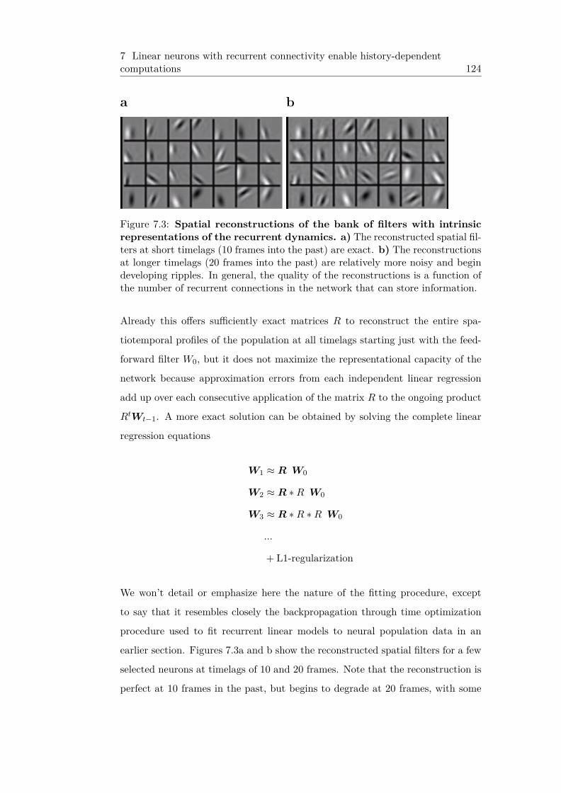
7 Linear neurons with recurrent connectivity enable history-dependentcomputations 124
a b
Figure 7.3: Spatial reconstructions of the bank of filters with intrinsicrepresentations of the recurrent dynamics. a) The reconstructed spatial fil-ters at short timelags (10 frames into the past) are exact. b) The reconstructionsat longer timelags (20 frames into the past) are relatively more noisy and begindeveloping ripples. In general, the quality of the reconstructions is a function ofthe number of recurrent connections in the network that can store information.
Already this offers sufficiently exact matrices R to reconstruct the entire spa-
tiotemporal profiles of the population at all timelags starting just with the feed-
forward filter W0, but it does not maximize the representational capacity of the
network because approximation errors from each independent linear regression
add up over each consecutive application of the matrix R to the ongoing product
RtWt−1. A more exact solution can be obtained by solving the complete linear
regression equations
W1 ≈ R W0
W2 ≈ R ∗R W0
W3 ≈ R ∗R ∗R W0
...
+ L1-regularization
We won’t detail or emphasize here the nature of the fitting procedure, except
to say that it resembles closely the backpropagation through time optimization
procedure used to fit recurrent linear models to neural population data in an
earlier section. Figures 7.3a and b show the reconstructed spatial filters for a few
selected neurons at timelags of 10 and 20 frames. Note that the reconstruction is
perfect at 10 frames in the past, but begins to degrade at 20 frames, with some

7 Linear neurons with recurrent connectivity enable history-dependentcomputations 125
a b
Figure 7.4: Properties of recurrent connections. a) The eigenvalue decom-position of the recurrent matrix shows a large number of eigenvalues close to 1,which result in long timescales in spatiotemporal filters. Such long timescales cangenerate spatial selectivity of a target cell at timelags of 10-20 frames and thusmaintain stimulus-information for extended periods of time.b) We can directlyinspect what pairs of neurons wire together by looking at their spatiotemporalreceptive fields. Neurons with similar preferred directions and orientations wiredtogether preferentially. The figure shows only the instantaneous receptive fieldsof 9 groups of neurons with the strongest connections to 9 target neurons (alwaysshown as the first neuron in the group). All neurons in the same group have simi-lar receptive field properties, and the target receptive field is a linear combinationof their receptive fields.
obvious rippling introduced into the filters. Eventually, the filters at long time-
lags degrade even more, but they do so in a relatively smooth manner, eventually
degrading to 0 because we have penalized the magnitude of the connections R.
We should also emphasize the particular fits shown in 7.3 have been performed
with large L1 regularization penalties on the parameters, for the purpose of ob-
taining a sparse R matrix with less than 5% overall connectivity (which may
more faithfully represent the regime of computation by realistic neural networks
in the cortex). Allowing full and unpenalized connectivity with as little as 1,024
neurons allowed the 1,024 by 1,024 matrix R to reconstruct almost any basis of
spatiotemporal filters we empirically tried. Can we learn anything from the ma-
trix of pairwise connections R determined in this fashion? Figure 7.4a shows the
eigenvalue spectrum of a typical matrix R fit with the optimization procedure

7 Linear neurons with recurrent connectivity enable history-dependentcomputations 126
detailed above. Most eigenvalues are relatively close to 1, which indicates long
timescales present in the dynamics of the linear recurrent network. The complex
parts of the eigenvalues show that the dynamics are not merely relaxing over time
but in fact gradually shifting the stimulus representation from one eigenvector to
its pair. Direction-selective simple cells have previously been proposed and im-
plemented with complex-valued basis functions by [Cadieu and Olshausen, 2009]
specifically to allow responses to rotate across the support vectors provided by the
instantaneous receptive field and its 90◦ phase-shifted pair. Our implementation
provides a more realistic representation in terms of scalar real-valued quantities
that can in fact be represented by the brain.
Figure 7.4b illustrates the types of neurons with large recurrent connections in the
matrix R. Each of the 9 groups of neurons shown represents the most strongly-
connected neurons to a target randomly chosen neuron (always shown as the
first neuron in the group). The figure shows only the spatial profiles of the con-
nected neurons, but a video of the timecourse of the receptive fields is available
at www.gatsby.ucl.ac.uk/marius. The video shows that not only neurons that
wire together have similar spatial receptive fields, but they also prefer similar
directions of motion. Intuitively, a Hebbian learning rule would account for such
connectivity patterns in cortex, although the rest of the paper shows that the
details of the connectivity patterns need to be slightly more complicated to allow
visual motion direction estimation. Neurons connecting strongly need to prefer
similar directions of motion, and to be spatially aligned in the direction of pre-
ferred motion of the presynaptic neuron. More details will be provided towards
the end of this chapter.
7.2.1 Complexity order for recurrent networks versus feed-
forward filters
Floating point operations per second (FLOPS) are an objective measure of the
efficiency of an algorithm. We use a similar measure to estimate the efficiency
of computing spatiotemporal neural responses from spatiotemporal visual stim-

7 Linear neurons with recurrent connectivity enable history-dependentcomputations 127
uli. Note that matters of efficiency are extremelly important in vision. The raw
amount of visual information available to the senses far exceeds even the compu-
tational capacity of the brain and only by selective attention (not discussed in this
thesis) can it be well encoded by the brain. Neurons in the fovea and up to 5◦ of
the visual field represent less than 1◦ portions of visual space, and many columns
of neurons need to be replicated throughout striate visual cortex to cover the
entire visual space. Finally, direction-selectivity is just one of the many functions
of V1 neurons. Orientation selectivity, color processing and spatial invariance are
also qualities of images that are important for visual perception.
Suppose the spatiotemporal filters are lx by ly by nt in size (space x space x
time, a typical example would be 12 x 12 x 30). A full V1 column may employ
a number on the order of N = 1,024 spatiotemporal filters. The number of
feedforward operations necessary to compute the dot-product between the filters
and the feedfoward input is thus 2Nl2xl2ynt. In contrast, the number of recurrent
operations necessary for the same computation is 2N2 + 2Nl2xl2y. The second
term in this sum is smaller than the number of feedforward operations by a
factor of nt, which could be up to 30 (assuming 5ms bins and history-dependence
for up to 150ms in the past). The first term may in principle be large, but
as discussed above recurrent connectivity in cortex is sparse, hence the total
number of non-zero connections in the matrix R may be a small fraction of all
possible connections, reducing 2N2 to 2pN2 with p the probability of connection
between all pairs of neurons. Sparse connectivity does not impair the quality of
the representation, because only neurons with similar spatio-temporal receptive
fields need to be wired together.
We thus see that the computational complexity of recurrent neural networks is
much reduced compared to simple linear spatiotemporal filters. This advantage
mimics the advantage offered by so-called IIR (infinite impulse response) filters
over FIR (finite impulse response) filters well-known in the signal processing
literature.
The second efficiency concern to any algorithm is its memory requirement. Mod-

7 Probabilistic Recurrent Neural Networks 128
ern computational hardware improves primarily by making memory access more
efficient, and the brain’s parallel computational hardware has often been thought
to be efficient mostly through its distributed memory systems and the band-
width of information that travels within and across brain areas continuously. A
quick calculation shows that that the memory requirements of recurrent networks
are straightforwardly nt times less than feedforward algorithms, simply because
lagged copies of stimulus inputs need to be stored at all.
Another algorithmic advantage to the recurrent network is its relatively small
number of parameters. If these parameters are indeed learned or optimized to the
statistics of the natural world, then an algorithm with the fewest free parameters
would be optimized most quickly and efficiently, and would be able to generalize
better to never-before-seen images and sequences of images.
Given the significant computational advantages of using a recurrent network to
compute visual motion properties, and given that the brain already has the neces-
sary hardware to implement it (i.e. recurrent connections), it would be surprising
if such a solution was not implemented in the brain.
7.3 Probabilistic Recurrent Neural Networks
In this section we introduce the binary-gated Gaussian recurrent neural network
as a generative model of sequences of images. This model belongs to the class
of nonlinear dynamical systems. Inference methods in such models typically
require expensive variational [Minka, 2001] or sampling based approximations
[Doucet et al., 2000], but we found that a low cost online filtering method works
sufficiently well to learn an interesting model. We begin with a description of
binary-gated Gaussian sparse coding for still images and then describe how to
define the dependencies in time between variables.

7 Probabilistic Recurrent Neural Networks 129
a
zt
xt
ht
yt
pτx
W, τy
b
zt
xt
ht
yt
ht+1
zt−1
t
R,bτx
W, τy
. . .. . .
Figure 7.5: The relationships between variables (neural activities, im-ages/retinal activities) in the graphical models used. a) Graphical modelrepresentation of the generative model of still images. b) Graphical model rep-resentation of the bgG-RNN with two consecutive time slices. The square boxrepresents that the variable zt is not random, but is given by zt = xt ◦ ht. Theparameters describe mean activities and connectivity parameters.
7.3.1 Binary Gated Gaussian Sparse Coding (bgG-SC).
Binary-gated Gaussian sparse coding (also called spike-and-slab sparse coding
[Goodfellow et al., 2012] may be seen as a limit of sparse coding with a mixture
of Gaussians priors [Olshausen and Millman, 2000] where one mixture compo-
nent has zero variance. Mathematically, the data yt is obtained by multiplying
together a matrix W of basis filters with a vector ht ◦ xt, where ◦ denotes the
operation of Hadamard or element-wise product, xt ∈ RN is Gaussian and spher-
ically distributed with standard deviation τx and ht ∈ {0, 1}N is a vector of
independent Bernoulli-distributed elements with success probabilities p. Finally,
small amounts of isotropic Gaussian noise with standard deviation τy are added
to produce yt.
For notational consistency with the dynamic version of this model, the t super-
script indexes time. The joint log-likelihood is
LtSC =− ‖yt −W · (ht ◦ xt)‖2/2τ2y − ‖xt‖2/2τ2
x+
+N∑j=1
(htj log pj + (1− htj) log (1− pj)
)+ const, (7.1)

7 Probabilistic Recurrent Neural Networks 130
where N is the number of basis filters in the model. By using appropriately
small activation probabilities p, the effective prior on ht ◦ xt can be made arbi-
trarily sparse. Probabilistic inference in sparse coding is intractable but efficient
variational approximation methods exist. We use a very fast approximation to
MAP inference, the matching pursuit algorithm (MP) [Mallat and Zhang, 1993].
Instead of using MP to extract a fixed number of coefficients per patch as usual,
we extract coefficients for as long as the joint log-likelihood increases. Patches
with more complicated structure will naturally require more coefficients to code.
Once values for xt and ht are filled in, the gradient of the joint log likelihood with
respect to the parameters is easy to derive. Note that xtk for which htk = 0 can
be integrated out in the likelihood, as they receive no contribution from the data
term in 7.1. Due to the MAP approximation, only the W can be learned. There-
fore, we set τ2x , τ
2y to reasonable values, both on the order of the data variance.
We also adapted pk during learning so that each filter was selected by the MP
process a roughly equal number of times. This helped stabilise learning, avoiding
a tendency to very unequal convergence rates.
When applied to whitened small patches from images, the algorithm produced
localized Gabor-like receptive fields as usual for sparse coding, with a range of
frequencies, phases, widths and aspect ratios. We found that when we varied
the average number of coefficients recruited per image, the receptive fields of the
learned filters varied in size. For example with only one coefficient per image,
a large number of filters represented edges extending from one end of the patch
to the other. With a large number of coefficients, the filters concentrated their
mass around just a few pixels. With even more coefficients, the learned filters
gradually became Fourier-like.
During learning, we gradually adapted the average activation of each variable htkby changing the prior activation probabilities pk. For 16x16 patches in a twice
overcomplete SC model (number of filters = twice the number of pixels), we
found that learning with 10-50 coefficients on average prevented the filters from
becoming too much or too little localized in space.

7 Probabilistic Recurrent Neural Networks 131
7.3.2 Binary-Gated Gaussian Recurrent Neural Network
(bgG-RNN).
To obtain a dynamic hidden model for sequences of images {yt} we specify the
following conditional probabilities between hidden chains of variables ht,xt:
P(xt+1,ht+1|xt,ht
)= P
(xt+1
)P(ht+1|ht ◦ xt
)P(xt+1
)= N
(0, τ2
x I)
P(ht+1|ht ◦ xt
)= σ
(R ·
(ht ◦ xt
)+ b
), (7.2)
where R is a matrix of recurrent connections, b is a vector of biases and σ is
the standard sigmoid function σ(a) = 1/(1 + exp(−a)). Note how the xt are
always drawn independently while the conditional probability for ht+1 depends
only on ht ◦ xt. We arrived at these designs based on a few observations. First,
similar to inference in SC, the conditional dependence on ht ◦ xt, allows us to
integrate out variables xt,xt+1 for which the respective gates in ht,ht+1 are 0.
Second, we observed that adding Gaussian linear dependencies between xt+1
and xt ◦ ht did not modify qualitatively the results reported here. However,
dropping P(ht+1|ht ◦ xt
)in favor of P
(xt+1|ht ◦ xt
)resulted in a model which
could no longer learn a direction-selective representation. For simplicity we chose
the minimal model specified by 7.2. The full log likelihood for the bgG-RNN is
LbgG-RNN =∑t
LtbgG-RNN where
LtbgG-RNN = const− ‖yt −W(xt ◦ ht)‖2/2τ2y − ‖xt‖2/2τ2
x+
+N∑j=1
htj log σ(R(ht−1 ◦ xt−1
)+ b
)j
+ (1− htj) log (1− σ(R(ht−1 ◦ xt−1
)+ b
)j), (7.3)
where x0 = 0 and h0 = 0 are both defined to be vectors of zeros.
7 Probabilistic Recurrent Neural Networks 132
7.3.3 Inference and learning of bgG-RNN.
The goal of inference is to set the values of xt, ht for all t in such a way as to
minimize the objective set by 7.3. Assuming we have already set xt, ht for t = 1 to
T , we propose to obtain xT+1, hT+1 exclusively from xT , hT . This scheme might
be called greedy filtering. In greedy filtering, inference is causal and Markov with
respect to time. At step T + 1 we only need to solve a simple SC problem given
by the slice LT+1bgG-RNN of the likelihood 7.3, where xT ,hT have been replaced
with the estimates xT , hT . The greedy filtering algorithm proposed here scales
linearly with the number of time steps considered and is well suited for online
inference. The algorithm may not produce very accurate estimates of the global
MAP settings of the hidden variables, but we found it was sufficient for learning
a complex bgG-RNN model. In addition, its simplicity coupled with the fast MP
algorithm in each LtbgG-RNN slice, resulted in very fast inference and consequently
fast learning. In most scenarios we learned models in under 30 minutes on a
standard quad core workstation.
Due to our approximate inference scheme, some parameters in the model had
to be set manually. These are τ2x and τ2
y , which control the relative strengths
in the likelihood of three terms: the data likelihood, the smallness prior on the
Gaussian variables and the interaction between sets of xt,ht consecutive in time.
In our experiments we set τ2y equal to the data variance and τ2
x = 2τ2y . We found
that such large levels of expected observation noise were necessary to drive robust
learning in R.
For learning we initialized parameters randomly to small values and first learned
W exclusively. Once the filters converge, we turn on learning for R. W does
not change very much beyond this point. We found learning of R was sensitive
to learning rate. We set the learning rate to 0.05 per batch, used a momentum
term of 0.75 and batches of 30 sets of 100 frame sequences. We whitened images
with a center-surround filter and normalized the mean and variance of whitened
pixel values in the training images to 0 and 1 respectively.
Gradients required for learning R show similarities to the STDP learning rule

7 Results 133
used in [Abbott and Blum, 1996] and [Rao and Sejnowski, 2000].
∂LtbgG-RNN∂Rjk
=(ht−1k xt−1
k
)·(htj − σ
(R(ht ◦ xt
)+ b
)j
). (7.4)
We will assume for neural interpretation that the positive and negative values
of xt ◦ ht are encoded by different neurons. If for a given neuron xt−1j is always
positive, then the gradient 7.4 is only positive when ht−1j = 1 and hti = 1 and
negative when ht−1j = 1 and hti = 0. In other words, the connection Rij is
strengthened when neuron j appears to cause neuron k to activate and inhibited
if neuron j fails to activate neuron k. A similar effect can be observed for the
negative part of xt−1j . This kind of Hebbian rule is widespread in cortex for long
term learning and is used in previous computational models of neural sequence
learning that partly motivated our work [Rao and Sejnowski, 2000].
7.4 Results
For data, we selected 100 short 100 frame long clips from a high resolution BBC
wildlife documentary. Clips were chosen only if they seemed on visual inspection
to have sufficient motion energy over the 100 frames. The clips chosen ended
up being mostly panning shots and close-ups of animals in their natural habitats
(the closer the camera is to a moving object, the faster it appears to move).
The results presented below measure the ability of the model to produce responses
similar to those of neurons recorded in primate experiments. The stimuli used in
these experiments are typically of two kinds: drifting gratings presented inside
circular or square apertures or translating bars of various lengths. These two
kinds of stimuli produce very clear motion signals, unlike motion produced by
natural movies. In fact, most patches we used in training contained a wide range
of spatial orientations, most of which were not orthogonal to the direction of local
translation. After comparing model responses to neural data, we finish with an
analysis of the connectivity pattern between model neurons that underlies their
responses.

7 Results 134
a b
Figure 7.6: a) Snapshot of nature documentary used for learning the statistics ofnatural movies. b) Four samples of the sequences of patches extracted from thedocumentary.
7.4.1 Measuring responses in the model.
We first had to deal with the potential negativity of the variables in the model,
since neural responses are always positive quantities. We decided to separate
the positive and negative parts of the Gaussian variables into two distinct sets
of responses. This interpretation is relatively common for sparse coding models
and we also found that in many units direction selectivity was enhanced when
the positive and negative parts of xt were separated (as opposed to taking the
absolute value for example). The enhancement was supported by a particular
pattern of network connectivity which we describe in a later subsection.
Additionally, since our inference procedure is deterministic, it will produce the
exact same response to the same stimulus every time. We added Gaussian noise
to the spatially whitened test image sequences, partly to capture the noisy envi-
ronments in cortex and partly to show robustness of direction selectivity to noise.
The amount of noise added was about half the expected variance of the stimulus.
7.4.2 Direction selectivity and speed tuning.
Direction selectivity is measured with the following index: DI = 1−Ropp/Rmax.
Here Rmax represents the response of a neuron in its preferred direction, while

7 Results 135
Ropp is the response in the direction opposite to that preferred. This selectivity in-
dex is commonly used to characterize neural data. To define a neuron’s preferred
direction, we inferred latent coefficients over many repetitions of square gratings
drifting in 24 directions, at speeds ranging from 0 to 3 pixels/frame in 0.25 steps.
The periodicity of the stimulus was twice the patch size, so that motion locally
appeared as an advancing long edge. The neuron’s preferred direction was the
direction in which it responded most strongly, averaged over all speeds. Once a
preferred direction was established, we defined the neuron’s preferred speed, as
the speed at which it responded most strongly in its preferred direction. Finally,
at this preferred speed and direction, we calculated the DI of the neuron. Similar
results were obtained if we averaged over all speed conditions.
We found that most neurons in the model had sharp tuning curves and direction-
selective responses. We cross validated the value of the direction index with a
new set of responses to obtain an average DI of 0.65, with many neurons having
a DI close to 1 (see figure 7.7c). 714 of 1,024 neurons were classified as direction-
selective on the basis of having DI > 0.5. Distributions of direction indices
and optimal speeds are shown in figure 7.7c. A neuron’s preferred direction was
always close to orthogonal to the axis of its Gabor receptive field, except for a few
degenerate cases around the edges of the patch. We defined the population tuning
curve as the average of the tuning curves of individual neurons, each aligned by
their preferred direction of motion. The DI of the population was 0.66. Neurons
were also speed tuned, in that responses could vary greatly and systematically as
a function of speed and DI was non-constant as a function of speed (see figure
7.7b). Usually at low and high speeds the DI was 0, but in between a variety
of responses were observed. Speed tuning is also present in recorded V1 neurons
[Orban et al., 1986], and could form the basis for global motion computation
based on the intersection of constraints method [Simoncelli and Heeger, 1998].

7 Results 136
a b
Speed (pix/frame)0 3R
espo
nse
preferred non-preferred
c
0 1 2 30
50
100
150
Num
ber
of u
nits
Preferred Speed (pix/frame)
0 0.5 10
100
200
Num
ber
of u
nits
Direction Index
d
Figure 7.7: Properties of the learned representations: static receptivefields, speed tuning, direction index and pairwise connectivities. a)Population of static filters derived by the model. b) Speed tuning of 16 randomlychosen neurons. Note that some neurons only respond weakly without motion,some are inhibited in the non-preferred direction compared to static responsesand most have a clear peak in the preferred direction at specific speeds. c)Top: Histogram of direction selectivity indices. Bottom: Histogram of preferredspeeds. d) For each of the 10 strongest excitatory connections per neuron we plotan asterisk indicating the orientation selectivity of pre and post-synaptic units.Note that most of the points are within π/4 from the diagonal, an area markedby the black lines. Note also the relatively increased frequency of horizontal andvertical edges.

7 Results 137
7.4.3 Vector velocity tuning
To get a more detailed description of single-neuron tuning, we investigated re-
sponses to different stimulus velocities. Since drifting gratings only contain mo-
tion orthogonal to their orientation, we switched to small (1.25pix x 2pix) drifting
Gabors for these experiments. We tested the network’s behavior with a full set
of 24 Gabor orientations, drifting in a full set of 24 directions with speeds rang-
ing from 0.25 pixels/frame to 3 pixels/frame, for a total of 6912 = 24 x 24 x 12
conditions with hundreds of repetitions of each condition. For each neuron we
isolated its responses to drifting Gabors of the same orientation travelling at the
12 different speeds in the 24 different directions. We present these for several
neurons in polar plots in figure 7.8c. Note responses tend to be high to vector
velocities lying on a particular line. In the next section we show that these are
the so called constraint lines.
7.4.4 Connectomics in silico
We had anticipated that the network would learn direction selectivity via specific
patterns of recurrent connection, in a fashion similar to the toy model studied in
Rao and Sejnowski [Rao and Sejnowski, 2000]. We now show that the pattern of
connectivity indeed supports this computation.
The most obvious connectivity pattern, clearly visible for single neurons in figure
7.8b, shows that neurons in the model excite other neurons in their preferred
direction and inhibit neurons in the opposite direction. This asymmetric wiring
naturally supports direction selectivity in combination with the second pattern
described below. This connectivity pattern emerges gradually during learning,
as shown in figure 7.9, a feature apparent in snapshots of the connectivity at the
beginning, middle and end of learning.
We find that asymmetry is not sufficient for direction selectivity to emerge —
strong excitatory projections also have to connect neurons with similar preferred
orientations and similar preferred directions. Only then will direction information

7 Results 138
propagate in the network in the identities of the active variables. We considered
the 10 strongest excitatory outputs for each neuron and calculated the expected
deviation between the orientation of these outputs and the orientation of the root
neuron. The average deviation was 23o, half the expected deviation if connections
were random. Figure 7.7d shows a raster plot of the pairs of orientations. The
same pattern held when we considered the strongest excitatory inputs to a given
neuron with an expected deviation of orientations of 24o. We could not directly
measure if neurons connected together according to direction selectivity because
of the sign ambiguity of xt variables. One can visually assess in figure 7.8b that
neurons connected asymmetrically with respect to their RF axis, but did they
also respond to motion primarily in that direction? As can be seen in figure 7.8c,
they did indeed. Since direction tuning is a measure of the incoming connections
to the neuron, we can qualitatively assess recurrence primarily connected together
neurons with similar direction preferences.
We also observed that neurons mostly projected strong excitatory outputs to
other neurons that were aligned parallel to the root neuron’s main axis (visible in
figures 7.8b). This is reminiscent of the aperture problem: locally all edges appear
to translate parallel to themselves. A neuron X with a preferred direction v and
preferred speed s has a so-called constraint line (CL), parallel to the Gabor’s
axis. When the neuron is activated by an edge E, the constraint line is formed
by all possible future locations of edge E that are consistent with global motion
in the direction v with speed s. Due to the presence of long contours in natural
scenes, the activation of X can predict at the next time step the activations of
other neurons with RFs aligned on the CL. Our likelihood function encourages
the model to learn to make such predictions as well as it can, and it indeed
discovers to use the constraint line solution. To quantify the degree to which
connections were made along a CL, for each neuron we fit a 2D Gaussian to
the distribution of RF positions of the 20 most strongly connected neurons, each
further weighted by its strength (the filled red circles in figure 7.8b). The major
axis of the Gaussians represent the constraint lines of the root neuron and are
in 862 out of 1024 neurons less than 15o away from perfectly parallel to the root

7 Discussion 139
neurons’ axis. The distance of each neuron to their constraint line was on average
1.68 pixels.
Yet perhaps the strongest manifestation of the CL tuning property of neurons in
the model can be seen in their responses to small stimuli drifting with different
vector velocities. Many of the neurons in figure 7.8c respond best when the
velocity vector ends on the constraint line and a similar trend holds for the aligned
population average.
It is already known from experiments of axon mappings simultaneous with dye-
sensitive imaging that neurons in V1 are more likely to connect with neurons
of similar orientations situated as far away as 4 mm / 4-8 minicolumns away
[Skaggs and McNaughton, 1997]. The model presented here makes three further
predictions: that neurons connect more strongly to neurons in their preferred
direction, that connected neurons lie on the constraint line and that they have
similar preferred directions to the root neuron.
7.5 Discussion
We have shown that a network of recurrently-connected neurons can learn to
discriminate motion direction at the level of individual neurons. Online greedy
filtering in the model is a sufficient approximate-inference method to produce
direction-selective responses. Fast, causal and online inference is a necessary
requirement for practical vision systems (such as the brain) but previous visual-
motion models did not provide such an implementation of their inference al-
gorithms. Another shortcoming of these previous models is that they obtain
direction selectivity by having variables with different RFs at different time lags,
effectively treating time as a third spatial dimension. A dynamic generative model
may be more suited for online inference with such methods such as particle filter-
ing, assumed density filtering, or the far cheaper method employed here of greedy
filtering.
The model neurons can be interpreted as predicting the motion of the stimulus.
7 Discussion 140
The lateral inputs they receive are however not sufficient in themselves to produce
a response, the prediction also has to be consistent with the bottom-up input.
When the two sources of information disagree, the network compromises but not
always in favor of the bottom-up input, as this source of information might be
noisy. This is reflected by the decrease in reconstruction accuracy from 80%
to 60% after learning the recurrent connections. It is tempting to think of V1
direction selective neurons as not only edge detectors and contour predictors
(through the nonclassical RF) but also predictors of future edge locations, through
their specific patterns of connectivity.
The source of direction selectivity in cortex is still an unresolved question, but
note that in the retina of non-primate mammals it is known with some certainty
that recurrent inhibition in the non preferred direction is largely responsible for
the direction selectivity of retinal ganglion cells [Fried et al., 2005]. It is also
known that, unlike orientation and ocular dominance, direction selectivity re-
quires visual experience to develop [Li et al., 2006], perhaps because direction
selectivity depends on a specific pattern of lateral connectivity unlike the largely
feedforward orientation and binocular tuning. Another experiment showed that
after many exposures to the same moving stimulus, the sequence of spikes trig-
gered in different neurons along the motion trajectory was also triggered in the
complete absence of motion, again indicating that motion signals in cortex may
be generated from lateral connections [Xu et al., 2012].
Thus, we see a number of reasons to propose that direction selectivity in the
cortex may indeed develop and be computed through a mechanism analagous to
the one we have developed here. If so, then experimental tests of the various
predictions developed above should prove to be revealing.
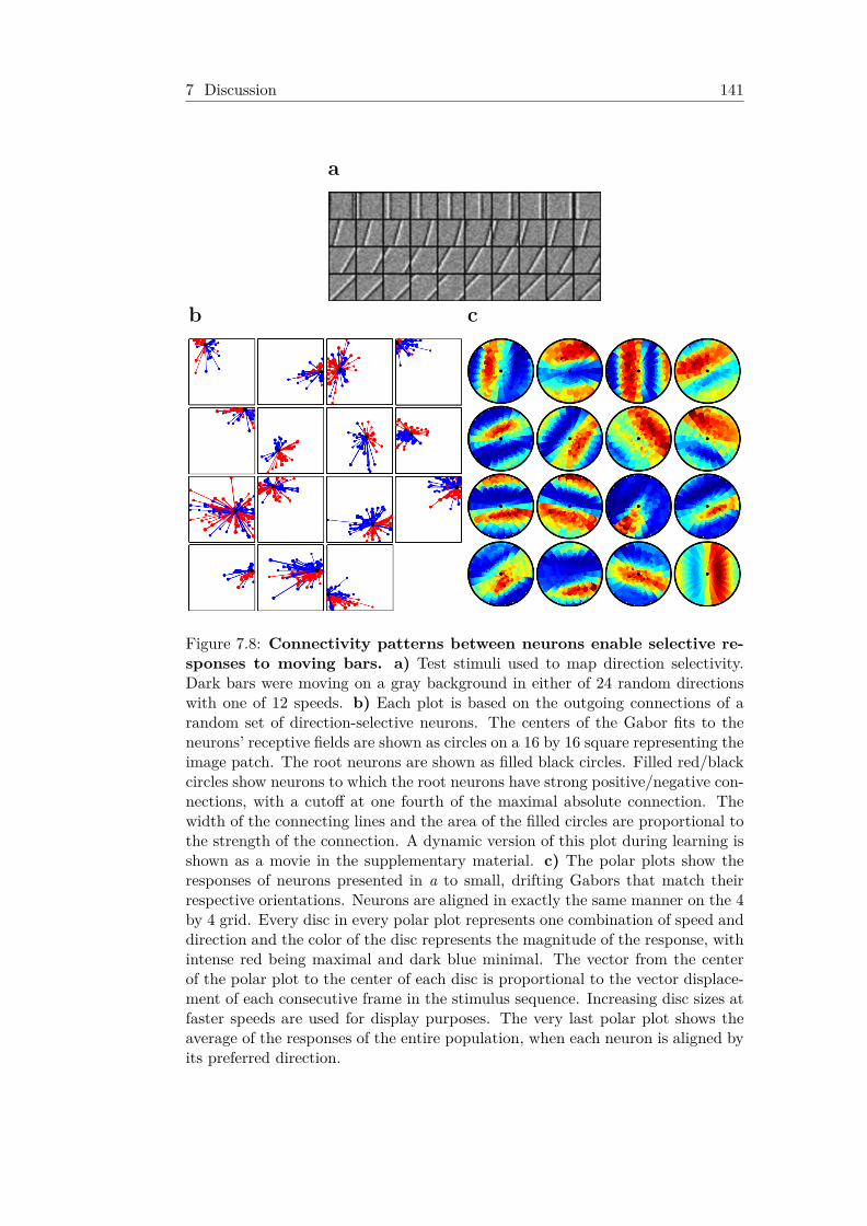
7 Discussion 141
a
b c
Figure 7.8: Connectivity patterns between neurons enable selective re-sponses to moving bars. a) Test stimuli used to map direction selectivity.Dark bars were moving on a gray background in either of 24 random directionswith one of 12 speeds. b) Each plot is based on the outgoing connections of arandom set of direction-selective neurons. The centers of the Gabor fits to theneurons’ receptive fields are shown as circles on a 16 by 16 square representing theimage patch. The root neurons are shown as filled black circles. Filled red/blackcircles show neurons to which the root neurons have strong positive/negative con-nections, with a cutoff at one fourth of the maximal absolute connection. Thewidth of the connecting lines and the area of the filled circles are proportional tothe strength of the connection. A dynamic version of this plot during learning isshown as a movie in the supplementary material. c) The polar plots show theresponses of neurons presented in a to small, drifting Gabors that match theirrespective orientations. Neurons are aligned in exactly the same manner on the 4by 4 grid. Every disc in every polar plot represents one combination of speed anddirection and the color of the disc represents the magnitude of the response, withintense red being maximal and dark blue minimal. The vector from the centerof the polar plot to the center of each disc is proportional to the vector displace-ment of each consecutive frame in the stimulus sequence. Increasing disc sizes atfaster speeds are used for display purposes. The very last polar plot shows theaverage of the responses of the entire population, when each neuron is aligned byits preferred direction.

7 Discussion 142
a b c
Figure 7.9: Connectivity changes during learning. a) We initialized thenetwork with random connections between neurons. bc) During learning, con-nections gradually sparsify and become asymmetric between the two sides of thereceptive fields of each cell.

VIII
Conclusion
We have developed statistical models that incorporate notions of dynamics and
fitted these models directly to recorded multi-neuron data from motor and sen-
sory cortices. Our approach bridges two existing computational methods in neu-
roscience: the relatively old tradition of computer simulations of networks and
the newer model-based data fitting techniques.
Computer simulations are essential exploratory tools in neuroscience but they
are often not well constrained by data. Simulation studies usually show that
networks of neurons can reproduce certain properties reported in the literature,
but many choices of parameters and network structure can also reproduce those
same properties. With the recent advent of large-scale simulation studies, it
seems the space of possible network parameters can increase in an unconstrained
fashion.
We reason that the only way to meaningfully develop large-scale simulations of
networks will be to directly fit all aspects of existing neurophysiological record-
ings. Much information about cortical networks is transparent in the temporal
timecourses of different neural classes to varied inputs. While these details of
the dynamics or of the receptive fields might be hard to describe explicitly and

8 144
quantitatively, they can nonetheless be crucial information for statistically iden-
tifying the underlying network structure that generated them. The approach we
suggest in this work uses all available data to fit network models that capture
the statistical structure of the data, which in turn has been generated by real
neuronal networks in the brain.
Note that other data fitting techniques have been developed to capture the shared
variability in multi-neuron recordings ([Pillow et al., 2008]). However, the ap-
proach of [Pillow et al., 2008] as well as those of [Schneidman et al., 2005] and
[Machens et al., 2010] lack the necessary network structure which allows us to
interpret the fitted models and simulate them as dynamical networks. Most
existing techniques for this purpose assume direct connections or interactions be-
tween neurons, yet most pairs of neurons in any brain area are not connected,
and the functional connectivity between cell pairs is an indirect consequence of
their participation in coordinated local network dynamics. Furthermore, fully
pairwise-connected approaches to data modelling quickly run into the curse of
dimensionality. The number of pairwise functional interactions scales quadrati-
cally with the number of recorded neurons, however the recording times usually
remain the same, being typically constrained by the qualities of the biological
preparation or the motivation of the animals.
We used the statistical network models to extract the underlying dynamical pat-
terns of cortical responses in auditory cortex and formulated hypothesis about
the cortical regimes of computation based on the inferred dynamics. Cortical net-
works in the synchronized state appear to be depression-stabilized, while network
responses in the desynchronized state are consistent with an inhibition-stabilized
regime. Previous work has studied such networks and showed that depression-
stabilized networks agree with many observations of auditory cortex structure,
while inhibition-stabilized networks may capture properties of the visual cor-
tex ([Loebel et al., 2007], [Murphy and Miller, 2009]). We found that these two
regimes can be exhibited by the same brain area in the same species in responses
to the same stimuli, but under different brain states. It is thus possible that neu-
ral networks are more heterogeneous than thought across brain areas and species,

8 145
but dynamical properties differ much more depending on brain state.
Indeed, in our respective preparations of the synchronized and desynchronized
states in auditory cortex, we find strong evidence that the networks are sta-
bilized by depression and inhibition respectively. Furthermore, we showed that
depression-stabilized networks are inherently unstable to small perturbations. De-
pression is simply too slow to act as an effective negative feedback loop and an
activated state can only be reset to quiescence by quick depletion of all the vesicles
in the network. The dynamics of depression-stabilized networks are dominated by
a single runaway excitatory mode which activates the entire population regardless
of the qualities of the external stimulus and indeed even spontaneously.
Our statistical model fits identified the runaway excitatory mode of the network
and also recovered a second excitatory mode closely-aligned with the first one and
paired with it dynamically. The two trajectories together account for the stereo-
typical sequence of firing observed in the synchronized state. Activity packets,
sometimes called population spikes, were shown to evolve dynamically and reli-
ably across a two-dimensional space of tightly-aligned eigenvectors.
Such dynamics have been described in the past to explain large transient re-
sponses at stimulus onsets, but these studies have suggested the non-normal
dynamics to be generated in a pair of excitatory and inhibitory populations
([Murphy and Miller, 2009]). Our model fits to the synchronized state suggests
instead that both response modes or populations have excitatory effects on the
network. Fast-spiking putative inhibitory neurons did not align with the late
mode of dynamics; in fact their activity slightly preceded the average RS ac-
tivity. Inhibitory interactions are still required for non-normal dynamics such
that the second excitatory mode can inhibit the first one. A candidate class of
interneurons for such interactions, likely not recorded in our experiments, are
somatostatin-positive neurons, which have been shown before to have late onsets
to auditory stimuli. In contrast, parvalbumin-positive neurons (likely FS cells in
our dataset) have faster onsets to external stimuli than RS cells.
These two-dimensional dynamics dominate the statistical response properties of

8 146
the network, greatly restricting the network capacity to encode stimuli. In con-
trast, the desynchronized network state appears to have much more flexible and
high-dimensional response properties and can thus encode sensory stimuli more
reliably. This is likely due to an overall increased ratio of inhibition to excitation,
which was also observed in awake rodents ([Haider et al., 2013]). The ratio of
recorded spikes of FS neurons to spikes of RS neurons was much greater in the
desynchronized brain state than in the synchronized.
We showed in simulations that increased inhibitory neuron activity can tran-
sition a network state from synchronized to desynchronised, or equivalently,
from depression-stabilized to inhibition-stabilized. Furthermore, in inhibitory-
stabilized networks we reproduced a key property of the desynchronized state,
namely that there are almost no noise correlations or trial-to-trial shared vari-
ability. Unlike depression-stabilized networks, an inhibition-stabilized network is
robust to small perturbations due to the very fast negative feedback loop pro-
vided by inhibition, and the effect of small perturbations decays exponentially
with the timescale of the excitatory and inhibitory conductances. Inhibition-
stabilized networks clearly provide better coding properties not only due to the
lack of trial-to-trial variability, but also because the inhibition balances the domi-
nant excitatory response mode of the network, allowing other dynamical response
modes to activate.
But are there any dynamics at all in the desynchronized state? To show that there
are intracortical dynamics in the desynchronized state, we analyzed the dynamics
of the neural responses to sustained tones and to random frequency-modulated
noise sweeps with very short temporal autocorrelation. Neural responses had
different properties in the desynchronized state, indicative of specific interactions
between the FS and RS populations. The early transients to tone onsets were
restricted to the FS population, suggesting that the increased effectiveness of
the inhibitory neurons shuts off the early sensory responses of the much slower
to respond putative excitatory neurons (RS). Late onset peaks in the sustained
responses of both FS and RS neurons are consistent with an intra-cortical or
local network origin of these responses. The late peak of the FS neurons was not

8 Emerging technologies for large-scale recordings 147
present in the synchronized state, consistent with a lack of effective inhibition
30ms after stimulus onset.
Neural responses to random FM sweeps had long (50-100ms) autocorrelation
properties despite stimuli being temporally uncorrelated at time lags of 10 ms or
more. In contrast, subcortical responses did not have such long temporal autocor-
relation. Having argued for the presence of dynamics in the desynchronized state,
we fitted statistical dynamical models to speech-evoked responses. We found that
the dimensionality of the fitted models was relatively high, and patterns of re-
sponses in spontaneous activity explained little of the response properties of the
network to stimulation.
8.1 Emerging technologies for large-scale
recordings
Over the past several decades, neural recording technologies have improved dra-
matically. In particular, the ability to monitor large, even complete populations
with single neuron resolution is now becoming a reality with techniques like high-
density electrophysiological probes and optical imaging. What challenges do the
new recordings pose from a data analysis point of view and more importantly
what new science can be conducted using them? While these questions may be
best answered in practice, for the rest of this thesis we speculate and suggest
possible applications.
Our analysis of chapter 4 suggested that animals in desynchronized brain states
may encode relatively high-dimensional stimulus inputs. However many of the
higher dimensions were very small compared to leading stimulus-encoding pro-
jections. Recording a larger number of neurons would allow a better ability to
look at the small-variance signals in the brain, because these signals are dis-
tributed over the population and can be demixed from the multi-neuron activity
with hidden Markov models such as the ones we have described here. Nothing
so far suggests that the relevant brain computations are performed at a large,

8 Emerging technologies for large-scale recordings 148
clearly-visible scale. In fact, the most large-scale signals that we currently see
in recordings are synchronized periods of whole-population activity that are not
linked to stimulus parameters or even to behavior (the animals are asleep).
Recording a large number of neurons simultaneously while animals are behav-
ing would also enable more efficient single-trial analysis. Most electrophysiology
studies still rely on averaging neural activity over trials, even when it is clear that
a large amount of variability exists from trial to trial and is lost in the average.
Instead, we suggest that in the future single trials of behavior will already be
analyzed for important information by effectively averaging the neural activity
over neurons instead of over trials. Neurons recorded often respond with similar
spiking to other neurons, hence averaging the activity of a population would al-
low tracking their collective behavior closely. However, no neuron performs the
exact same computation as another neuron. The underlying neural dynamics
are distributed across the population and mixed together. The role of statistical
models is then to demix the different sources of inputs and variability so as to
find the weighted projections with most relevant information about the stimulus,
the network computation or the behavior.
Another benefit of large-scale recordings may be to shed light on the noise that
has been assumed to be overly-present in the brain. Single spikes are thought to
occur with noisy timing and often be missed completely, but it may be possible
to explain single spikes from the activity of all the other neurons in the local
population. For example, recording all presynaptic sources of a neuron’s dendritic
input should in principle allow much better spike-level prediction than currently
possible and may reveal computations that single neurons are performing.
Continuing the line of thought of the previous paragraph, recording the activity
of a complete neural population may allow us to recover the actual connectome
of pairwise connectivity. Currently the recovered functional connectivity from
population recordings does not capture actual physical connections but only the
distributions of common inputs that most pairs of neurons receive. Recovering
physical connectivity from spiking responses will require recording an entire pop-

8 Emerging technologies for large-scale recordings 149
ulation with spike-level accuracy, so that no external common inputs can alter the
correlation structure, because all the common inputs are within the recordings.

Bibliography
[Abbott and Blum, 1996] Abbott, L. and Blum, K. (1996). Functional signifi-
cance of long-term potentiation for sequence learning and prediction. Cerebral
Cortex, 6:406–416. (pages 117 and 133)
[Abolafia et al., 2013] Abolafia, J., Martinez-Garcia, M., Deco, G., and Sanchez-
Vives, M. (2013). Variability and information content in auditory cortex spike
trains during an interval-discrimination task. Journal of Neurophysiology,
110:2163–74. (page 15)
[Aizenberg and Geffen, 2013] Aizenberg, M. and Geffen, M. N. (2013). Bidirec-
tional effects of aversive learning on perceptual acuity are mediated by the
sensory cortex. Nature Neuroscience, 16(8):994–6. (page 107)
[Allman et al., 1985] Allman, J., Miezin, F., and McGuinness, E. (1985). Stimu-
lus specific responses from beyond the classical receptive field: neurophysiolog-
ical mechanisms for local-global comparisons in visual neurons. Annual review
of neuroscience, 8(1):407–430. (page 14)
[Arieli et al., 1996] Arieli, A., Sterkin, A., Grinvald, A., and Aertsen, A. (1996).
Dynamics of ongoing activity: explanation of the large variability in evoked
cortical responses. Science, 273(5283):1868–71. (page 109)
[Atencio and Schreiner, 2013] Atencio, C. and Schreiner, C. (2013). Auditory
cortical local subnetworks are characterized by sharply synchronous activity.
Journal of Neuroscience, 33(47):18503–14. (pages 15 and 59)
8 BIBLIOGRAPHY 151
[Azouz and Gray, 2003] Azouz, R. and Gray, C. M. (2003). Adaptive Coincidence
Detection and Dynamic Gain Control in Visual Cortical Neurons In Vivo. Neu-
ron, 37:513–523. (page 109)
[Bandyopadhyay et al., 2010] Bandyopadhyay, S., Shamma, S. A., and Kanold,
P. O. (2010). Dichotomy of functional organization in the mouse auditory
cortex. Nature Neuroscience, 13:361–368. (page 14)
[Banerjee and Liu, 2013] Banerjee, S. B. and Liu, R. C. (2013). Storing ma-
ternal memories: hypothesizing an interaction of experience and estrogen on
sensory cortical plasticity to learn infant cues. Frontiers in Neuroendocrinology,
34(4):300–14. (page 107)
[Bao et al., 2004] Bao, S., Chang, E. F., Woods, J., and Merzenich, M. M. (2004).
Temporal plasticity in the primary auditory cortex induced by operant percep-
tual learning. Nature Neuroscience, 7(9):974–81. (page 107)
[Barber, 2002] Barber, D. (2002). Learning in spiking neural assemblies. Ad-
vances in Neural Information Processing, 15. (page 118)
[Bathellier et al., 2012] Bathellier, B., Ushakova, L., and Rumpel, S. (2012). Dis-
crete neocortical dynamics predict behavioral categorization of sounds. Neuron,
76(2):435–49. (pages 14, 96, and 109)
[Beltramo et al., 2013a] Beltramo, R., D’Urso, G., Dal Maschio, M., Farisello,
P., Bovetti, S., Clovis, Y., Lassi, G., Tucci, V., Tonelli, D. D. P., and Fellin,
T. (2013a). Layer-specific excitatory circuits differentially control recurrent
network dynamics in the neocortex. Nature neuroscience, 16(2):227–234.
(page 15)
[Beltramo et al., 2013b] Beltramo, R., D’Urso, G., Dal Maschio, M., Farisello,
P., Bovetti, S., Clovis, Y., Lassi, G., Tucci, V., Tonelli, D. D. P., and Fellin,
T. (2013b). Layer-specific excitatory circuits differentially control recurrent
network dynamics in the neocortex. Nature neuroscience, 16(2):227–234.
(page 59)

8 BIBLIOGRAPHY 152
[Berkes et al., 2009] Berkes, P., Turner, R., and Sahani, M. (2009). A structured
model of video produces primary visual cortical organisation. PLoS Computa-
tional Biology, 5. (page 118)
[Bermudez Contreras et al., 2013] Bermudez Contreras, E. J., Schjetnan, A.
G. P., Muhammad, A., Bartho, P., McNaughton, B. L., Kolb, B., Gruber,
A. J., and Luczak, A. (2013). Formation and reverberation of sequential neu-
ral activity patterns evoked by sensory stimulation are enhanced during cortical
desynchronization. Neuron, 79(3):555–66. (pages 90, 92, and 105)
[Bishop, 2006] Bishop, C. M. (2006). Pattern Recognition and Machine Learning.
Springer. (page 32)
[Brea et al., 2011] Brea, J., Senn, W., and Pfister, J. (2011). Sequence learning
with hidden units in spiking neural networks. Advances in Neural Information
Processing, 24. (page 118)
[Buesing et al., 2012] Buesing, L., Macke, J., and Sahani, M. (2012). Spectral
learning of linear dynamics from generalised-linear observations with applica-
tion to neural population data. Advances in Neural Information Processing
Systems, 25. (page 30)
[Buzsaki, 2004] Buzsaki, G. (2004). Large-scale recording of neuronal ensembles.
Nature Neuroscience, 7(5):446–51. (page 24)
[Cadieu and Olshausen, 2009] Cadieu, C. and Olshausen, B. (2009). Learning
transformational invariants from natural movies. Advances in Neural Informa-
tion Processing, 21:209–216. (pages 118 and 126)
[Cardin et al., 2009] Cardin, J., Carle, M., Meletis, K., Knoblich, U., Zhang,
F., Deisseroth, K., Tsai, L., and Moore, C. (2009). Driving fast-spiking cells
induces gamma rhythm and controls sensory responses. Nature, 459:663–7.
(page 59)
[Castro-Alamancos, 2009] Castro-Alamancos, M. (2009). Cortical up and acti-
vated states: implications for sensory information processing. The Neurosci-
entist, pages 625–634. (pages 102 and 108)

8 BIBLIOGRAPHY 153
[Castro-Alamancos, 2004a] Castro-Alamancos, M. A. (2004a). Absence of rapid
sensory adaptation in neocortex during information processing states. Neuron,
41(3):455–464. (page 90)
[Castro-Alamancos, 2004b] Castro-Alamancos, M. A. (2004b). Dynamics of sen-
sory thalamocortical synaptic networks during information processing states.
Progress in Neurobiology, 74(4):213–47. (page 89)
[Cavanaugh et al., 2002] Cavanaugh, J. R., Bair, W., and Movshon, J. A. (2002).
Nature and interaction of signals from the receptive field center and surround
in macaque v1 neurons. Journal of neurophysiology, 88(5):2530–2546. (page 14)
[Churchland et al., 2010] Churchland, M. M., Yu, B., and al (2010). Stimulus
onset quenches neural variability: a widespread cortical phenomenon. Nature
Neuroscience, 13(3):369–78. (page 48)
[Churchland et al., 2007] Churchland, M. M., Yu, B. M., Sahani, M., and Shenoy,
K. V. (2007). Techniques for extracting single-trial activity patterns from large-
scale neural recordings. Current Opinion in Neurobiology, 17(5):609–618.
(page 24)
[Cohen and Maunsell, 2009] Cohen, M. and Maunsell, J. (2009). Attention im-
proves performance primarily by reducing interneuronal correlations. Nature,
12:1594–1600. (page 59)
[Constantinople and Bruno, 2011] Constantinople, C. and Bruno, R. (2011). Ef-
fects and mechanisms of wakefulness on local cortical networks. Neuron,
69:1061–1068. (pages 15 and 59)
[Cooke et al., 2007] Cooke, J. E., Zhang, H., and Kelly, J. B. (2007). Detection
of sinusoidal amplitude modulated sounds: deficits after bilateral lesions of
auditory cortex in the rat. Hearing Research, 231(1-2):90–9. (page 107)
[Crochet and Petersen, 2006] Crochet, S. and Petersen, C. C. H. (2006). Cor-
relating whisker behavior with membrane potential in barrel cortex of awake
mice. Nature Neuroscience, 9(5):608–10. (page 89)

8 BIBLIOGRAPHY 154
[Curto et al., 2009] Curto, C., Sakata, S., Marguet, S., Itskov, V., and Harris,
K. D. (2009). A simple model of cortical dynamics explains variability and state
dependence of sensory responses in urethane-anesthetized auditory cortex. The
Journal of neuroscience, 29(34):10600–12. (pages 15, 92, 105, 107, and 109)
[Dayan and Abbott, 2001] Dayan, P. and Abbott, L. (2001). Theoretical Neuro-
science. The MIT Press. (page 118)
[de la Rocha et al., 2007] de la Rocha, J., Doiron, B., Shea-Brown, E., Josic, K.,
and Reyes, A. (2007). Correlation between neural spike trains increases with
firing rate. Nature, 448:802–806. (page 15)
[Destexhe et al., 2007] Destexhe, A., Hughes, S. W., Rudolph, M., and Crunelli,
V. (2007). Are corticothalamic ’up’ states fragments of wakefulness? Trends
in Neurosciences, 30(7):334–42. (pages 102 and 108)
[Destexhe et al., 2003] Destexhe, A., Rudolph, M., and Pare, D. (2003). The
high-conductance state of neocortical neurons in vivo. Nature Reviews Neuro-
science, 4:739–751. (page 63)
[Doucet et al., 2000] Doucet, A., Freitas, N., Murphy, K., and Russell, S. (2000).
Rao-blackwellised particle filtering for dynamic Bayesian networks. UAI’00
Proceedings of the Sixteenth conference on Uncertainty in artificial intelligence,
pages 176–183. (page 128)
[Douglas et al., 1995] Douglas, R., Koch, C., Mahowald, M., Martin, K., and
Suarez, H. (1995). Recurrent excitation in neocortical circuits. Science,
269(5226):981–985. (page 119)
[Ecker et al., 2014] Ecker, A. S., Berens, P., Cotton, R. J., Subramaniyan, M.,
Denfield, G. H., Cadwell, C. R., Smirnakis, S. M., Bethge, M., and Tolias, A. S.
(2014). State Dependence of Noise Correlations in Macaque Primary Visual
Cortex. Neuron, 82(1):235–248. (pages 15 and 108)
[Eliades and Wang, 2008] Eliades, S. and Wang, X. (2008). Neural substrates of
vocalization feedback monitoring in primate auditory cortex. Nature, 453:1102–
06. (page 59)

8 BIBLIOGRAPHY 155
[Elman, 1990] Elman, J. (1990). Finding structure in time. Cognitive Science,
14:179–211. (page 29)
[Ferster and Miller, 2000] Ferster, D. and Miller, K. D. (2000). Neural mecha-
nisms of orientation selectivity in the visual cortex. Annual Review of Neuro-
science, 23(1):441–471. (page 14)
[Fried et al., 2005] Fried, S., Munch, T., and Werblin, F. (2005). Directional
selectivity is formed at multiple levels by laterally offset inhibition in the rabbit
retina. Neuron, 46(1):117–127. (page 140)
[Friston, 1999] Friston, K. (1999). A theory of cortical responses. Phil. Trans.
R. Soc. B, 360(1456):815–836. (page 119)
[Gabernet et al., 2005] Gabernet, L., Jadhav, S. P., Feldman, D. E., Carandini,
M., and Scanziani, M. (2005). Somatosensory integration controlled by dy-
namic thalamocortical feed-forward inhibition. Neuron, 48:315–327. (page 16)
[Garcia-Lazaro et al., 2013] Garcia-Lazaro, J. A., Belliveau, L. A. C., and Lesica,
N. A. (2013). Independent population coding of speech with sub-millisecond
precision. The Journal of Neuroscience, 33(49):19362–72. (page 95)
[Giraud and Poeppel, 2012] Giraud, A.-L. and Poeppel, D. (2012). Cortical os-
cillations and speech processing: emerging computational principles and oper-
ations. Nature Neuroscience, 15(4):511–7. (page 109)
[Goard and Dan, 2009] Goard, M. and Dan, Y. (2009). Basal forebrain activation
enhances cortical coding of natural scenes. Nature Neuroscience, 12(11):1444–
9. (pages 15 and 90)
[Goodfellow et al., 2012] Goodfellow, I., Courville, A., and Bengio, Y.
(2012). Spike-and-slab sparse coding for unsupervised feature discovery.
arXiv:1201.3382v2. (page 129)
[Greenberg et al., 2008] Greenberg, D. S., Houweling, A. R., and Kerr, J. N. D.
(2008). Population imaging of ongoing neuronal activity in the visual cortex
of awake rats. Nature Neuroscience, 11(7):749–51. (page 89)

8 BIBLIOGRAPHY 156
[Gu et al., 2011] Gu, Y., Liu, S., Fetsch, C., Yang, Y., Fok, S., Sunkara, A.,
DeAngelis, G., and Angelaki, D. (2011). Perceptual learning reduces interneu-
ronal correlations in macaque visual cortex. Neuron, 71(4):750–61. (page 59)
[Guo et al., 2012] Guo, W., Chambers, A. R., Darrow, K. N., Hancock, K. E.,
Shinn-Cunningham, B. G., and Polley, D. B. (2012). Robustness of cortical
topography across fields, laminae, anesthetic states, and neurophysiological
signal types. The Journal of Neuroscience, 32(27):9159–72. (page 90)
[Haider et al., 2013] Haider, B., Hausser, M., and Carandini, M. (2013). Inhi-
bition dominates sensory responses in the awake cortex. Nature, 493:97–100.
(pages 15, 59, and 146)
[Haider and McCormick, 2009] Haider, B. and McCormick, D. a. (2009). Rapid
neocortical dynamics: cellular and network mechanisms. Neuron, 62(2):171–89.
(page 89)
[Hamilton et al., 2013] Hamilton, L., Sohl-Dickstein, J., Huth, A., Carels, V.,
Deisseroth, K., and Bao, S. (2013). Optogenetic activation of an inhibitory
network enhances feedforward functional connectivity in auditory cortex. Na-
ture, 80:1066–76. (page 59)
[Han and Mrsic-Flogel, 2013] Han, Y. and Mrsic-Flogel, T. (2013). A finely tuned
cortical amplifier. Nature Neuroscience, 16(9):1166–1168. (page 14)
[Harris and Thiele, 2011] Harris, K. D. and Thiele, A. (2011). Cortical state and
attention. Nature Reviews Neuroscience, 12(9):509–23. (pages 89, 108, and 109)
[Hasenstaub et al., 2007] Hasenstaub, A., Sachdev, R. N. S., and McCormick,
D. a. (2007). State changes rapidly modulate cortical neuronal responsiveness.
The Journal of Neuroscience, 27(36):9607–22. (pages 90 and 109)
[Hirata and Castro-Alamancos, 2011] Hirata, A. and Castro-Alamancos, M. A.
(2011). Effects of cortical activation on sensory responses in barrel cortex.
Journal of Neurophysiology, 105(4):1495–505. (pages 15 and 90)

8 BIBLIOGRAPHY 157
[Horvath and Lesica, 2011] Horvath, D. and Lesica, N. A. (2011). The effects of
interaural time difference and intensity on the coding of low-frequency sounds
in the mammalian midbrain. The Journal of neuroscience : the official journal
of the Society for Neuroscience, 31(10):3821–7. (page 96)
[Hromadka et al., 2013] Hromadka, T., Zador, A. M., and DeWeese, M. R.
(2013). Up states are rare in awake auditory cortex. Journal of Neurophysiol-
ogy, 109:1989–1995. (page 74)
[Jones et al., 2001] Jones, H., Grieve, K., Wang, W., and Sillito, A. (2001). Sur-
round suppression in primate v1. Journal of Neurophysiology, 86(4):2011–2028.
(page 14)
[Kalman, 1960] Kalman, R. (1960). A new approach to linear filtering and pre-
diction problems. Journal of Basic Engineering, 82(1):35–45. (pages 21 and 24)
[Kaufman et al., 2014] Kaufman, M. T., Churchland, M. M., Ryu, S. I., and
Shenoy, K. V. (2014). Cortical activity in the null space: permitting prepara-
tion without movement. Nature Neuroscience, 17:440–448. (page 47)
[Kayser et al., 2009] Kayser, C., Montemurro, M. A., Logothetis, N. K., and
Panzeri, S. (2009). Spike-phase coding boosts and stabilizes information carried
by spatial and temporal spike patterns. Neuron, 61(4):597–608. (page 109)
[Kimura et al., 2014] Kimura, R., Sohya, K., Tsumoto, T., Safari, M., Mirnajafi-
Zadeh, J., Ebina, T., and Yanagawa, Y. (2014). Curtailing effect of awakening
on visual responses of cortical neurons by cholinergic activation of inhibitory
circuits. Journal of Neuroscience, 34(30):10122–33. (page 59)
[Lakatos et al., 2013] Lakatos, P., Musacchia, G., O’Connel, M. N., Falchier,
A. Y., Javitt, D. C., and Schroeder, C. E. (2013). The spectrotemporal filter
mechanism of auditory selective attention. Neuron, 77(4):750–61. (page 109)
[Latham et al., 2010] Latham, P. E., Richmond, B., Nelson, P., and Nirenberg, S.
(2010). Intrinsic dynamics in neuronal networks. Journal of Neurophysiology,
83(2):808–827. (page 15)

8 BIBLIOGRAPHY 158
[Li et al., 2013a] Li, L.-y., Li, Y.-t., Zhou, M., Tao, H. W., and Zhang, L. I.
(2013a). Intracortical multiplication of thalamocortical signals in mouse audi-
tory cortex. Nature Neuroscience, 16(9):1179–1181. (page 14)
[Li et al., 2006] Li, Y., FitzPatrick, D., and White, L. (2006). The development
of direction selectivity in ferret visual cortex requires early visual experience.
Nature Neuroscience, 9(5):676–681. (page 140)
[Li et al., 2013b] Li, Y.-t., Ibrahim, L. A., Liu, B.-h., Zhang, L. I., and Tao,
H. W. (2013b). Linear transformation of thalamocortical input by intracortical
excitation. Nature Neuroscience, 16(9):1324–1330. (page 14)
[Lien and Scanziani, 2013] Lien, A. D. and Scanziani, M. (2013). Tuned thalamic
excitation is amplified by visual cortical circuits. Nature Neuroscience. (page 14)
[Litwin-Kumar and Doiron, 2012] Litwin-Kumar, A. and Doiron, B. (2012). Slow
dynamics and high variability in balanced cortical networks with clustered
connections. Nature Neuroscience, 15:1498–1505. (page 17)
[Livingstone, 1998] Livingstone, M. (1998). Mechanisms of direction selectivity
in macaque V1. Neuron, 20:509–526. (page 117)
[Loebel et al., 2007] Loebel, A., Nelken, I., and Tsodyks, M. (2007). Processing
of sounds by population spikes in a model of primary auditory cortex. Frontiers
in Neuroscience, 1(1):197–209. (pages 15 and 144)
[London et al., 2010] London, M., Roth, A., Beeren, L., Hausser, M., and
Latham, P. (2010). Sensitivity to perturbations in vivo implies high noise
and suggests rate coding in cortex. Nature, 466:123–127. (page 65)
[Luczak et al., 2009] Luczak, A., Bartho, P., and Harris, K. D. (2009). Spon-
taneous events outline the realm of possible sensory responses in neocortical
populations. Neuron, 62(3):413–25. (pages 15, 59, 96, 99, and 109)
[Luczak et al., 2013] Luczak, A., Bartho, P., and Harris, K. D. (2013). Gating of
sensory input by spontaneous cortical activity. The Journal of Neuroscience,
33(4):1684–95. (pages 89, 90, 99, 107, and 109)

8 BIBLIOGRAPHY 159
[Machens et al., 2010] Machens, C. K., Romo, R., and Brody, C. D. (2010). Func-
tional, but not anatomical, separation of what and when in prefrontal cortex.
Journal of Neuroscience, 30(1):350–360. (page 144)
[Macke et al., 2011] Macke, J., Busing, L., Cunningham, J., Yu, B., Shenoy, K.,
and Sahani, M. (2011). Empirical models of spiking in neural populations.
Advances in Neural Information Processing Systems, 24:1350–1358.
(pages 24, 30, and 34)
[MacLean et al., 2005] MacLean, J. N., Watson, B. O., Aaron, G. B., and Yuste,
R. (2005). Internal dynamics determine the cortical response to thalamic stim-
ulation. Neuron, 48(5):811–23. (pages 15 and 109)
[Mallat and Zhang, 1993] Mallat, S. and Zhang, Z. (1993). Matching pursuits
with time-frequency dictionaries. IEEE Transactions on Signal Processing,
41(12):3397–3415. (page 130)
[Marguet and Harris, 2011] Marguet, S. L. and Harris, K. D. (2011). State-
dependent representation of amplitude-modulated noise stimuli in rat auditory
cortex. The Journal of Neuroscience, 31(17):6414–20.
(pages 15, 89, 90, 92, 105, and 107)
[Middleton et al., 2012] Middleton, J., Omar, C., Doiron, B., and Simons, D.
(2012). Neural correlation is stimulus modulated by feedforward inhibitory
circuitry. Jorunal of Neuroscience, 32(2):506–18. (page 15)
[Mikami et al., 1986] Mikami, A., Newsome, W., and Wurtz, R. (1986). Motion
selectivity in macaque visual cortex. II. Spatiotemporal range of directional
interactions in MT and V1. Journal of Neurophysiology, 55(6):1328–1339.
(page 117)
[Mikolov et al., 2011] Mikolov, T., Deoras, A., Kombrink, S., Burget, L., and
Cernocky, J. (2011). Empirical evaluation and combination of advanced lan-
guage modeling techniques. Conference of the International Speech Communi-
cation Association. (page 30)

8 BIBLIOGRAPHY 160
[Minka, 2001] Minka, T. (2001). Expectation propagation for approximate
Bayesian inference. UAI’01 Proceedings of the Seventeenth conference on Un-
certainty in artificial intelligence, pages 362–369. (page 128)
[Mitchell et al., 2009] Mitchell, J. F., Sundberg, K. A., and Reynolds, J. H.
(2009). Spatial attention decorrelates intrinsic activity fluctuations in macaque
area v4. Neuron, 63:879–888. (page 15)
[Murphy and Miller, 2009] Murphy, B. K. and Miller, K. D. (2009). Balanced
amplification: A new mechanism of selective amplification of neural activity
patterns. Neuron, 61:635–648. (pages 15, 144, and 145)
[Okun et al., 2012] Okun, M., Yger, P., Marguet, S. L., Gerard-Mercier, F., Be-
nucci, A., Katzner, S., Busse, L., Carandini, M., and Harris, K. D. (2012).
Population rate dynamics and multineuron firing patterns in sensory cortex.
The Journal of Neuroscience, 32(48):17108–19. (pages 59, 89, 92, and 105)
[Olshausen, 2003] Olshausen, B. (2003). Learning sparse, overcomplete repre-
sentations of time-varying natural images. IEEE International Conference on
Image Processing. (page 117)
[Olshausen and Millman, 2000] Olshausen, B. and Millman, K. (2000). Learning
sparse codes with a mixture-of-Gaussians prior. Advances in Neural Informa-
tion Processing, 12. (page 129)
[Orban et al., 1986] Orban, G., Kennedy, H., and Bullier, J. (1986). Velocity sen-
sitivity and direction selectivity of neurons in areas V1 and V2 of the monkey:
influence of eccentricity. Journal of Neurophysiology, 56(2):462–480. (page 135)
[Otazu et al., 2009] Otazu, G. H., Tai, L.-H., Yang, Y., and Zador, A. M. (2009).
Engaging in an auditory task suppresses responses in auditory cortex. Nature
Neuroscience, 12(5):646–54. (pages 15, 90, and 108)
[Pillow et al., 2008] Pillow, J. W., Shlens, J., Paninski, L., Sher, A., Litke,
A. M., Chichilnisky, E. J., and Simoncelli, E. P. (2008). Spatio-temporal cor-
relations and visual signalling in a complete neuronal population. Nature,
454(7207):995–999. (pages 24, 33, and 144)

8 BIBLIOGRAPHY 161
[Polack et al., 2013] Polack, P.-O., Friedman, J., and Golshani, P. (2013). Cel-
lular mechanisms of brain state-dependent gain modulation in visual cortex.
Nature neuroscience, 16(9):1331–9. (page 89)
[Porter et al., 2011] Porter, B. A., Rosenthal, T. R., Ranasinghe, K. G., and
Kilgard, M. P. (2011). Discrimination of brief speech sounds is impaired in
rats with auditory cortex lesions. Behavioural Brain Research, 219(1):68–74.
(page 107)
[Poulet and Petersen, 2008] Poulet, J. F. A. and Petersen, C. C. H. (2008). In-
ternal brain state regulates membrane potential synchrony in barrel cortex of
behaving mice. Nature, 454(7206):881–5. (page 89)
[Rao and DH, 1999] Rao, R. and DH, B. (1999). Predictive coding in the visual
cortex: a functional interpretation of some extra-classical receptive-field effects.
Nature Neuroscience, 2(1):79–87. (page 119)
[Rao and Sejnowski, 2000] Rao, R. and Sejnowski, T. (2000). Predictive sequence
learning in recurrent neocortical circuits. Advances in Neural Information Pro-
cessing, 12:164–170. (pages 117, 119, 120, 133, and 137)
[Reed et al., 2011] Reed, A., Riley, J., Carraway, R., Carrasco, A., Perez, C.,
Jakkamsetti, V., and Kilgard, M. P. (2011). Cortical map plasticity improves
learning but is not necessary for improved performance. Neuron, 70(1):121–31.
(page 107)
[Renart et al., 2010] Renart, A., de la Rocha, J., Bartho, P., Hollender, L., Parga,
N., Reyes, A., and Harris, K. D. (2010). The asynchronous state in cortical
circuits. Science (New York, N.Y.), 327(5965):587–90.
(pages 17, 72, 73, 107, and 108)
[Rigas and Castro-Alamancos, 2007] Rigas, P. and Castro-Alamancos, M. A.
(2007). Thalamocortical Up states: differential effects of intrinsic and ex-
trinsic cortical inputs on persistent activity. The Journal of Neuroscience,
27(16):4261–72. (page 109)

8 BIBLIOGRAPHY 162
[Ringach, 2009] Ringach, D. L. (2009). Spontaneous and driven cortical activity:
implications for computation. Current Opinion in Neurobiology, 19(4):439–44.
(page 109)
[Rothschild et al., 2010a] Rothschild, G., Nelken, I., and Mizrahi, A. (2010a).
Functional organization and population dynamics in the mouse primary audi-
tory cortex. Nature Neuroscience, 13:353–360. (page 14)
[Rothschild et al., 2010b] Rothschild, G., Nelken, I., and Mizrahi, A. (2010b).
Functional organization and population dynamics in the mouse primary audi-
tory cortex. Nature Neuroscience, 13:353–60. (page 59)
[Rumelhart et al., 1986] Rumelhart, D., Hinton, G., and Williams, R. (1986).
Learning internal representations by error propagation. Mit Press Computa-
tional Models Of Cognition And Perception Series, pages 318–462. (page 30)
[Sachidhanandam et al., 2013] Sachidhanandam, S., Sreenivasan, V., Kyri-
akatos, A., Kremer, Y., and Petersen, C. C. H. (2013). Membrane potential
correlates of sensory perception in mouse barrel cortex. Nature Neuroscience,
16(11):1671–7. (page 89)
[Sahani and Linden, 2003] Sahani, M. and Linden, J. (2003). How linear are
auditory cortical responses? In Becker, S., Thrun, S., and Obermayer, K.,
editors, Advances in neural information processing systems 15, pages 301–308,
Cambridge, MA. MIT. (page 96)
[Sakata and Harris, 2009] Sakata, S. and Harris, K. (2009). Laminar structure of
spontaneous and sensory-evoked population activity in auditory cortex. Neu-
ron, 64:404–18. (page 59)
[Sato et al., 2013] Sato, T. K., Hausser, M., and Carandini, M. (2013). Distal
connectivity causes summation and division across mouse visual cortex. Nature
neuroscience. (page 14)
[Sato et al., 2012] Sato, T. K., Nauhaus, I., and Carandini, M. (2012). Traveling
waves in visual cortex. Neuron, 75:218–229. (page 15)
8 BIBLIOGRAPHY 163
[Schneider et al., 2014] Schneider, D., Nelson, A., and Mooney, R. (2014). A
synaptic and circuit basis for corollary discharge in the auditory cortex. Nature,
513:189–194. (page 59)
[Schneidman et al., 2005] Schneidman, E., Berry, M., Segev, R., and Bialek, W.
(2005). Weak pairwise correlations imply strongly correlated network states in
a neural population. Nature, 440:1007–1012. (pages 24, 31, 34, and 144)
[Simoncelli and Heeger, 1998] Simoncelli, E. and Heeger, D. (1998). A model of
neuronal responses in visual area MT. Vision Research, 38(5):743–761.
(page 135)
[Skaggs and McNaughton, 1997] Skaggs, W. and McNaughton, B. (1997). Replay
of neuronal firing sequences in rat hippocampus during sleep following spatial
experience. Journal of Neuroscience, 17(6):2112–2127. (page 139)
[Song et al., 2006] Song, W.-J., Kawaguchi, H., Totoki, S., Inoue, Y., Katura,
T., Maeda, S., Inagaki, S., Shirasawa1, H., and Nishimura, M. (2006). Cortical
intrinsic circuits can support activity propagation through an isofrequency strip
of the guinea pig primary auditory cortex. Cerebral Cortex, 16:718–729.
(page 15)
[Steriade et al., 2001] Steriade, M., Timofeev, I., and Grenier, F. (2001). Natural
waking and sleep states: a view from inside neocortical neurons. Journal of
Neurophysiology, 85(5):1969–1985. (page 89)
[Sun et al., 2010] Sun, Y. J., Kim, Y.-J., Ibrahim, L. A., Tao, H. W., and Zhang,
L. I. (2010). Response features of parvalbumin-expressing interneurons suggest
precise roles for subtypes of inhibition in visual cortex. Neuron, 67(5):847–857.
(page 16)
[Sun et al., 2014] Sun, Y. J., Kim, Y.-J., Ibrahim, L. A., Tao, H. W., and Zhang,
L. I. (2014). Synaptic mechanisms underlying functional dichotomy between
intrinsic-bursting and regular-spiking neurons in auditory cortical layer 5. Jour-
nal of Neuroscience, 33(12):5326–5339. (page 15)
8 BIBLIOGRAPHY 164
[Tan et al., 2013] Tan, A., Andoni, S., and Priebe, N. (2013). A spontaneous
state of weakly correlated synaptic excitation and inhibition in visual cortex.
Neuroscience, 247:364–75. (page 15)
[Tan et al., 2014] Tan, A. Y. Y., Chen, Y., Scholl, B., Seidemann, E., and Priebe,
N. J. (2014). Sensory stimulation shifts visual cortex from synchronous to
asynchronous states. Nature. (pages 15 and 89)
[Ter-Mikaelian et al., 2007] Ter-Mikaelian, M., Sanes, D. H., and Semple, M. N.
(2007). Transformation of temporal properties between auditory midbrain
and cortex in the awake Mongolian gerbil. The Journal of Neuroscience,
27(23):6091–102. (page 90)
[van Vreewijk and Sompolinsky, 1996] van Vreewijk, C. and Sompolinsky, H.
(1996). Chaos in neuronal networks with balanced excitatory and inhibitory
activity. Science, 274(5293):1724–1726. (page 72)
[Wehr and Zador, 2005] Wehr, M. and Zador, A. (2005). Synaptic mechanisms
of forward suppression in rat auditory cortex. Nature, 47:437–445.
(pages 15, 16, and 63)
[Wetzel et al., 1998] Wetzel, W., Ohl, F. W., Wagner, T., and Scheich, H. (1998).
Right auditory cortex lesion in Mongolian gerbils impairs discrimination of ris-
ing and falling frequency-modulated tones. Neuroscience Letters, 252(2):115–8.
(page 107)
[Wiskott and Sejnowski, 2002] Wiskott, L. and Sejnowski, T. (2002). Slow fea-
ture analysis: Unsupervised learning of invariances. Neural Computation,
14(4):715–770. (page 118)
[Wolf et al., 2014] Wolf, F., Engelken, R., Puelma-Touzel, M., Weidinger, J.
D. F., and Neef, A. (2014). Dynamical models of cortical circuits. Current
Opinion in Neurobiology, 25:228–236. (page 15)
[Xu et al., 2012] Xu, S., Jiang, W., Poo, M.-M., and Dan, Y. (2012). Activity
recall in a visual cortical ensemble. Nature Neuroscience, 15(3):449–55, S1–2.
(pages 89 and 140)

8 BIBLIOGRAPHY 165
[Yu et al., 2006] Yu, B., Afshar, A., Santhanam, G., Ryu, S., Shenoy, K., and
Sahani, M. (2006). Extracting dynamical structure embedded in neural activity.
Advances in Neural Information Processing Systems, 18:1545–1552. (page 24)
[yun Li et al., 2014] yun Li, L., Xiong, X. R., Ibrahim, L. A., Yuan, W., Tao,
H. W., , and Zhang, L. I. (2014). Differential receptive field properties of
parvalbumin and somatostatin inhibitory neurons in mouse auditory cortex.
Cerebral Cortex, online. (pages 15 and 16)
[Zhang et al., 2014] Zhang, S., Xu, M., Kamigaki, T., Do, J. P. H., Chang, W.-
C., Jenvay, S., Miyamichi, K., Luo, L., and Dan, Y. (2014). Long-range and
local circuits for top-down modulation of visual cortex processing. science,
345(6197):660–665. (page 14)
[Zhou et al., 2014a] Zhou, M., Liang, F., Xiong, X. R., Li, L., Li, H., Xiao, Z.,
Tao, H. W., and Zhang, L. I. (2014a). Scaling down of balanced excitation and
inhibition by active behavioral states in auditory cortex. Nature Neuroscience,
(April). (pages 89 and 90)
[Zhou et al., 2014b] Zhou, Y., hua Liu, B., Wu, G. K., Kim, Y.-J., and Xiao,
Z. (2014b). Preceding inhibition silences layer 6 neurons in auditory cortex.
Neuron, 65:706–717. (page 15)
[Zion Golumbic et al., 2013] Zion Golumbic, E. M., Ding, N., Bickel, S., Lakatos,
P., Schevon, C. a., McKhann, G. M., Goodman, R. R., Emerson, R., Mehta,
A. D., Simon, J. Z., Poeppel, D., and Schroeder, C. E. (2013). Mechanisms
underlying selective neuronal tracking of attended speech at a ”cocktail party”.
Neuron, 77(5):980–91. (page 109)