neural basis underlying auditory categorization in …yslee/thesis_ysl.pdfneural basis underlying...
TRANSCRIPT

Neural basis underlying auditory categorization in the human brain
A Thesis
Submitted to the Faculty
in partial fulfillment of the requirements for
Doctor of Philosophy
in
Cognitive Neuroscience
by
Yune-Sang Lee
DARTMOUTH COLLEGE
Hanover, New Hampshire
May 2010
Examining Committee:
(Chair) Richard Granger
Jim Haxby
Elise Temple
Petr Janata
Brian W. Pogue, Ph.D.
Dean of Graduate Studies

Copyright by
Yune-Sang Lee
2010

!!"
Abstract
Our daily lives are pervaded by sounds, predominantly speech, music, and
environmental sounds. We readily recognize and categorize such sounds. Our
understanding of how the brain so effortlessly recognizes and categorizes sounds is still
rudimentary. The central focus of this thesis is elucidation of the neural mechanisms
underlying auditory categorization. To this end, the thesis mainly employed multivoxel
pattern-based analysis techniques (MVPA) applied to functional magnetic resonance
imaging (fMRI) data. The first study revealed differential neural patterns for the
representation of different auditory object categories (e.g., animate vs. inanimate at
superordinate level, human vs. dog at basic level). Importantly, the categorical neural
patterns were not just confined within the classical auditory cortex. Rather, we were able
to find the categorical responses throughout the brain beyond the early sensory area. A
second study revealed both auditory and visual responses to distinguish between animate
and inanimate categories within the same anatomical regions far downstream from the
early sensory cortex, suggesting that those areas may be involved in object processing
independent of modality. A third study identified melodic contour processing areas (e.g.,
rSTS, lIPL, and ACC) in the music domain. Neural patterns in these areas differ between
ascending and descending melodies. A fourth study revealed several left-lateralized
cortical loci where different phonetic categories were distinguished with differentiable
neural patterns. Further, the findings demonstrated that there was difference between
low-level vs. high-level speech processing regions in their role of simple acoustic feature
detection vs. complex categorical processing. Taken together, the findings presented in
this thesis provide evidence that the brain uses a unifying strategy - categorical neural

!!!"
response - for auditory categorization in all three sub-domains. Further, throughout the
studies, not only modality-specific but also modality-independent high-level processing
regions were often found for auditory processing. These findings may help us move
toward an improved understanding of how received signals progress from low-level
processing (e.g., frequency extraction) to high-level processing (e.g., understanding the
concept).

!#"
Preface
I have always been interested in music and spent a fair amount of my college
years playing guitar in a rock band and performing in clubs. After college, I decided to
become a professional musician, which led me to work as a commercial music director.
During that time, I became more engaged in and impressed by the powerful influence of
music on the human mind. Whenever I had free time, I tried to read articles and books
regarding music cognition, acoustics and auditory science. I finally decided to study
auditory neuroscience in graduate school.
This dissertation is the result of a five-year endeavor to answer the question of
how sound is processed by the brain. Instead of focusing on only one type of sound, I
hoped to broadly examine the auditory categorization occurring in environmental sounds,
speech sounds, and musical sounds. I also sought to find a unifying neural mechanism for
the perception of such different types of sounds. The recently developed fMRI
methodology of multivariate pattern analysis allowed me to address these questions and
make some intriguing discoveries: the brain appears to use the strategy of generating
differential neural patterns to distinguish different categories of sounds in dedicated
categorization areas, including the auditory cortex and other brain regions that vary
depending on the nature of sound. Further, the findings led me to the general conclusion
that a wide range of brain regions are engaged in turning a modality-specific signal into
modality-independent conceptual entity.

#"
Research on these issues is still in its infancy and it is exciting to be working on
many open questions. I hope the findings in my thesis will serve as a useful contribution
to this rapidly growing field.
Acknowledgements
I would like to thank those who have been helpful with my thesis work. First of
all, I would like to express my deepest gratitude to my advisor Dr. Richard Granger and
three other committee members including Dr. Jim Haxby, Dr. Elise Temple, and Dr. Petr
Janata. Without their advice, guidance, and suggestions, this work would not have been
feasible. I also offer special thanks to Dr. Peter Tse and Dr. Rajeev Raizada for their
tremendous amount of help with my research and academic career. I would like to thank
lab members: Melissa Rundle, Sergey Fogelson, Amy Palmer, Stephanie Gagnon,
Geethmala Sridaran, Carlton Frost and Samuel Lloyd. Lastly, I would like to extend my
deepest appreciation to my wife, Sun Choung for her perpetual support, encouragement,
and patience, and for my two children, Dong-Ha (River) and Jung-Ha (Jamie).

#!"
Table of contents
List of Tables…………………………………………………………………………...viii
List of Illustrations ……………………………………………………………………...ix
Chapter 1. General Introduction …………………………………………………...…..1
Chapter 2. Neural basis underlying environmental sounds categorization ………..14
Experiment 1……………………………………………………………………...….15
Introduction …………………………………………………………………………...16
Methods ………………………………………………………………………...….….18
Results ……………………………………………………………………..………….26
Discussion …………………………………………………………………………….39
Experiment 2…………………………………………………………….….………..43
Introduction ………………………………………………………………..….……....44
Methods …………………………………………………………………..…………...44
Results …………………………………………………………………….………..…50
Discussion ………………………………………………………………………….…60
Chapter 3. Neural basis underlying melodic contour categorization ………….....…64
Introduction …………………………………………………………………………...65
Methods ……………………………………………………………………….....……67

#!!"
Results ……………………………………………………………………………...…73
Discussion ………………………………………………………………………….....82
Chapter 4. Neural basis underlying speech phoneme categorization ………………89
Introduction ………………………………………………………………………...…90
Methods ………………………………………………………………………….……94
Results …………………………………………………………………………...……98
Discussion …………………………………………………………………...………103
Chapter 5. General Discussion ……………………………………………….………110
Implication of the findings in the thesis ……………………………………………..111
GLM versus MVPA ………………………………………………………..………..117
Distributed vs. localized brain mechanism …………………………………….........120
The rationale of choosing threshold …………………………………………………121
Chapter 6. Conclusions ……………………………………………………….……...125
Appendix ………………………………………………………………………………128
References ………………………………………………………………………..……134

#!!!"
List of Tables
Table 1. List of brain regions for basic (animate) level …………………………………29
Table 2. List of brain regions for basic (animate) level …………………………………30
Table 3. List of brain regions for superordinate level (intact sounds) ………………......34
Table 4. List of brain regions for superordinate level (inverted sounds) ………………..35
Table 5. List of brain regions for visual categorization ………………………………....54
Table 6. List of brain regions for auditory categorization ……………………………....55
Table 7. List of brain regions for audio-visual categorization …………………………..56
Table 8. List of brain regions for melodic-contour categorization ……………………...79
Table 9. List of brain regions for phoneme categorization ………….............................102
Table 10. Descriptive statistics of spectral centroid of animate and inanimate
sounds …………………………………………………………………………..128
Table 11. 20 stimulus pairs for the pitch-screening task ………………………………131
Table 12. The results of post-hoc t-test for each pair-wise comparison on the four melody
categories ………………………………………………………………….........133

!$"
List of illustrations
"
Figure 1. Conventional paradigm in univariate General Linear Modeling analysis……....7
Figure 2. Differential neural patterns on the visual object categories within the ventral
temporal lobes ………………………………………………………………..…...9
Figure 3. Schematic illustration of multivariate fMRI paradigm ……………………….10
Figure 4. Differential neural patterns on the auditory object categories within the superior
temporal lobes………………………………………………………………...….12
Figure 5. Schematic dendrogram of stimuli set (Top) Experimental design (Bottom)….20
Figure 6. Spectrograms of intact and inverted cat sound…………………………….…..21
Figure 7. Sound identification results at the basic-level sounds ………………………...27
Figure 8. Brain regions that participate in basic (animate) level……………………...…27
Figure 9. Temporal-lobe close-up of animate and inanimate specific regions ………….28
Figure 10. Sound identification results at the superordinate level ……………………... 32
Figure 11. Brain regions participating in superordinate categorization ……………..…..33
Figure 12. The group results of GLM showing the areas that were more activated by all
the sounds (animate & inanimate) than by baseline…………………………..…37
Figure 13. The group results of GLM comparing animate and inanimate categories of
intact sounds………………………………………………………………....…..38
Figure 14. The group results of GLM comparing animate and inanimate categories of
inverted sounds…………………………………………………………………..39
Figure 15. The lateral view of brain areas that distinguish between animate and inanimate
categories in each modality………………………………………………………52
Figure 16. Representative brain regions containing auditory and visual responses……..53

$"
Figure 17. Group map of GLM results showing the areas that were more activated by
auditory stimuli than by visual stimuli and vice versa ………………………..…58
Figure 18. Group map of GLM results comparing animate vs. inanimate categories of
images……………………………………………………………………………59
Figure 19. Group map of GLM results comparing animate vs. inanimate categories of
sounds……………………………………………………………………………60
Figure 20. Staff view of the 20 melodies generated using MIDI software……………....68
Figure 21. Schematic illustration of ascending and descending melodies……………….69
Figure 22. Happiness ratings for the four melody categories……………………………74
Figure 23. Happiness ratings for ascending and descending melodies…………….…….74
Figure 24. Happiness ratings for major and minor melodies…………………………….75
Figure 25. Multi-dimensional scaling structure on the similarity distance among all
Pair-wise melody comparisons……………………………………………..……76
Figure 26. Brain regions that distinguish between ascending and descending melodic
Sequences………………………………………………………………………...78
Figure 27. The result of whole brain searchlight analysis between major and minor
Melodies……………………………………………………………………….…79
Figure 28 Group results of GLM showing areas more activated during melody conditions
than during rest…………………………………………………………......……81
Figure 29. Group result of GLM comparing ascending to descending melodies………..81
Figure 30. Group result of GLM comparing major to minor melodies………………….82
Figure 31. The spectrogram of token 1 (/ba/) and token 10 (/da/)……………………….95

$!"
Figure 32. Psychometric function curve on the phonetic continuum from /ba/ to /da/ that
were acquired and averaged across 11 native English speaker…………………..99
Figure 33. Group results of GLM showing areas more activated during the phoneme
listening conditions than during the rest……………………………………..…100
Figure 34. Group results of MVPA (top) and GLM (bottom) showing areas that
distinguish between /ba/ and /da/……………………………………………….101
Figure 35. Group results of MVPA……………………………………………………..102
Figure 36. Anterior right superior temporal region comparison………………………..113
Figure 37. Right superior temporal sulcus comparison………………...………………115
Figure 38. Mean spectral centroid comparison between animate and inanimate sounds in
intact and inverted sound condition………………………………………….…129
Figure 39. Ratio of responses among three categorization levels for the sound
identification task………………………………………………………………130
Figure 40. 4 odd-ball melodies…………………………………………………………132
Figure 41. Psychometric function curves on the phonetic continuum that were acquired
from 11 native English speakers………………………………………………..133

!"
Chapter 1.
General Introduction

!"
Background and significance
In everyday life, we are exposed to various environmental sounds, human speech,
and music. We can readily recognize and categorize each of those sounds. Importantly,
the recognition of certain sounds (a fire alarm, screeching brakes) can be a matter of life
or death. In many ways, recognition and categorization of auditory cues is just as crucial
as recognition and categorization of visual cues, and there is often interplay between the
two modalities. Yet auditory categorization has received substantially less attention than
visual categorization in the scientific literature. Many dominant hypothesis of object
categorization originate in the field of vision, such as hierarchical organization (Jolicoeur
et al., 1984). The theory of hierarchical organization was postulated from observations
that reaction time was faster and more accurate at the “basic” level (e.g., dog), while
slower and less accurate at superordinate (e.g., animal) and subordinate (e.g., poodle)
levels. Based on the reaction time difference among different categorization levels, the
theory has suggested that objects may be first recognized at basic-level (entry level),
which is followed by superordinate and subordinate level.
Are there any neurophysiology studies supporting such a notion? Recently,
single-cell recordings in macaque, human EEG (Electroencephalography), and MEG
(magentoencephalography) studies have consistently reported two major peaks in neural
activity while subjects perform an object categorization task, an earlier peak (100 ~ 135
ms) that reflects basic-level (coarse-grained) and a later peak (160 ~ 300 ms) that reflects
subordinate level (fine-grained) categorization, suggesting sequential categorization
(Sugase et al., 1999; Johnson et al., 2003; Scott et al., 2006; Liu et al., 2002).

!"
Interestingly, the earlier peak reflects basic-level (coarse-grained) categorization and later
peak reflects subordinate level (fine-grained) categorization.
For example, in a single-cell recording study (Sugase et al., 1999), two rhesus
monkeys viewed various expressions of human and rhesus faces while the activity of
cells in the inferior temporal areas was recorded. The authors conjectured that differential
responses to human and monkey faces would reflect basic-level categorization, and
differential responses for facial expressions would reflect subordinate level
categorization. The results showed that the early peak (117ms) contained the global
information of human or monkey faces and the late peak (165ms) contained the specific
information of various facial expression in both human and monkey faces, demonstrating
basic-level categorization preceding subordinate categorization by approximately 50ms
during the visual recognition processing in the ITG.
An MEG study (Liu et al., 2002) also suggested that the early MEG signal
component (M100) and late MEG signal component (M170) were independently
modulated by basic-level categorization and subordinate level categorization
respectively. In this study, the experimenters first presented face and house pictures to
subjects while measuring MEG signals. They found that the MEG signal in the FFA area
had two major peaks for the face pictures but not for the house pictures. Subsequently
subjects performed an object categorization task (face vs. house) and face identification
task (face A vs. face B) with slightly scrambled images. Early and late MEG peaks were
bigger for successful object categorization while only the late MEG peak was bigger for
successful face categorization, indicating fine-grained subordinate categorization follows
objects categorization at the basic level.

!"
Similarly, a recent EEG study (Scott et al., 2006) showed that subordinate level
categorization training only enhanced the late ERP (Event Related Potential) component
(N250), while basic-level categorization training enhanced both early (N170) and late
ERP components. Together, these neurophysiological findings support the theory of
hierarchical organization of visual categorization.
An additional aspect of the hypothesis is that basic level is the “entry” level of
processing. But are objects always recognized at the basic level? Some studies have
suggested that objects can also be directly recognized at the subordinate level by experts
in a domain (Tanaka et al., 1991; Gauthier et al., 2000). Tanaka et al. (1991) measured
the reaction time of bird and dog experts while they performed an animal categorization
task at both a basic and a subordinate level. Intriguingly, subjects’ reaction times were
not different between basic and subordinate level categorizations in their domain of
expertise but subjects’ reaction times were significantly slower at the subordinate level of
a novice domain (e.g., categorizing different birds for dog experts and different dogs for
birds experts). This seminal study suggested that the “entry level” of categorization can
be shifted from a basic to a subordinate level, depending on level of expertise.
All of these findings were made mostly in the visual domain, which led us to the
question: Is auditory categorization processing analogously organized? Adams and Janata
(2002) tested both auditory and visual categorization at the basic and subordinate level.
The results showed that subjects were faster and more accurate at basic than at
subordinate levels independent of modality, suggesting that the hierarchical organization
of auditory categorization processing may resemble that of visual categorization
processing. They continued their investigation of modality-independent categorization
!"
processing with an fMRI study using the same task. By comparing visual vs. auditory
activation, they found evidence that object categorization in each modality was mainly
mediated by modality-specific sensory areas. Further, a comparison between subordinate
and basic-level categorization suggested the involvement of some additional areas such
as the inferior frontal lobe for both auditory and visual categorization at subordinate
level, suggesting that more neural substrates are recruited in order to process finer-level
categorization.
Other studies have found that different portions of the superior temporal cortex
are more activated by a particular auditory object category (Belin & Zatorre, 2000; Lewis
et al., 2005). Belin and Zatorre (2000) found that the anterior superior temporal sulcus
(aSTS) was more activated by the human voice than by environmental sounds, and
claimed that the aSTS is the FFA (Fusiform Face Area) of the auditory domain. More
recently, Lewis and colleagues (2005) showed that bilateral middle superior temporal
gyri were activated more by animate sound categories than by inanimate sound
categories. These two studies clearly suggested that humans’ auditory cortex is tuned to
conspecific sounds either at superordinate level (e.g., animate as opposed to inanimate) or
at basic level (e.g., human voice as opposed to other animate sounds).
In addition to the environmental sound categorization, there are other distinct
auditory sub-domains, including speech and music. Importantly, there is also unique
categorization processing in both speech and music domains. A notable example is
categorical speech perception. This phenomenon was first found by Liberman et al.
(1957) in the late 1950s. Their study demonstrated that phonetic sounds created by
morphing two prototype phonemes were categorically perceived with a sharp perceptual

!"
boundary between categories despite linear variation in acoustic structure along a
phonetic. Since its discovery, the phenomenon of categorical phoneme perception has
been replicated by numerous studies not only with adults, but also with human infants
(Eimas et al., 1971) and non-human primates (Kuhl & Padden, 1983). For example, Kuhl
and Padden (1983) trained non-human primates to distinguish prototypes among /ba/,
/da/, and /ga/ sounds with go/no-go paradigm such that the animals were required to
respond to only /da/ phonetic sound. Later, the animals were presented with morphed
versions of /ba/, /da/, and /ga/ phonemes and, like humans, they perceived those
phonemes categorically.
Musical melodies also appear to be categorically perceived. A study (Johnsrude et
al., 2000) showed that patients with right temporal lobe lesions were not able to
distinguish between ascending and descending contour of two tones, but they were
reliably able to distinguish if those tones were the same or different. This finding
suggested that tone extraction and melodic contour processing might be processed
independently. Further, it is conceivable that these processes might be hierarchically
organized such that tone extraction is followed by melodic contour processing by
concatenating those extracted tones at higher level.
As stated above, there is some behavioral evidence that each domain of sound
(environmental sounds, speech, and music) is categorically perceived. Yet, it appears that
the underlying neural mechanisms may not have been entirely addressed by the
prevailing univariate GLM (General Linear Model) analysis method. GLM studies
explicitly assume and test that different categories are processed by ‘additive’ or
‘suppressive’ BOLD (Blood-Oxygen-Level-Dependent) activity at a given region. Figure
!"
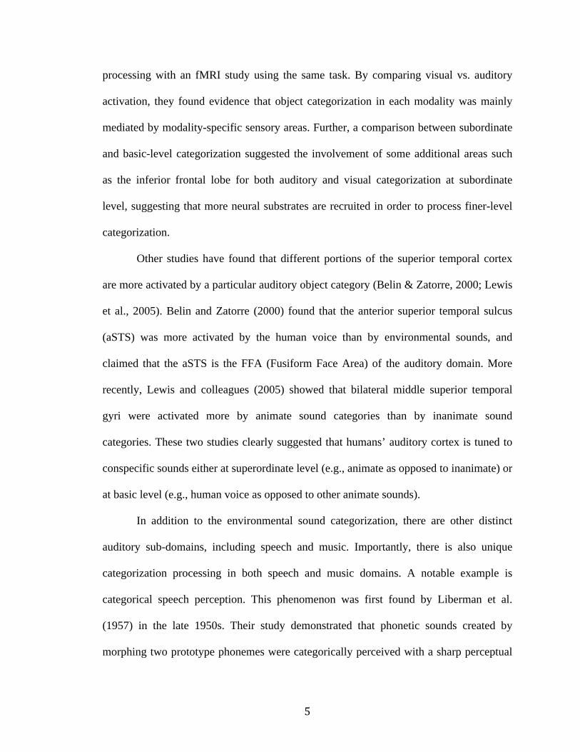
1 illustrates the paradigm of a typical univariate GLM anylsis. Suppose a hypothetical
case in which a particular auditory area responds to both ‘cat’ and ‘dog’ sounds and we
want to know whether the area responds differentially to those sounds. In univariate
GLM, the amplitude of BOLD activity in one condition (cat sounds) is compared to the
activity in another condition (dog sounds) on a voxel-by-voxel basis.
Figure 1. Conventional paradigm in univariate General Linear Modeling (GLM)
analysis The BOLD activity driven by each sound is predicted by estimating the
regression coefficient (B value) per every voxel. The estimated B value is directly
compared between two conditions (cat vs. dog) and tested if they are significantly
different from each other at a particular voxel.
If the amplitude of BOLD activity in a given voxel is reliably different from one
condition to another, we might conclude that that the response of that voxel distinguishes
between categories. Further, if a group of voxels in a particular area is preferentially
activated by a particular category (e.g., dog sounds) more than any other category, we
might conclude that this area is dedicated to the perception of that category. This
technique has proved helpful in a number of experiments, including neuroimaging studies

!"
that have found several functional “modules” such as the fusiform face area (Kanwisher
et al., 1998) or parahippocampal place area (Epstein & Kanwisher, 1997).
However, although we can behaviorally distinguish thousands of different objects,
only a few areas have been suggested to be preferentially activated by specific categories.
The brain may not just use the strategy of quantitative modulation of neuronal activity per
every single object. A study by Haxby and colleagues (2001) suggested another feasible
neural mechanism of object categorization. The experimenters presented eight different
categories of visual images during fMRI scans. They then calculated the correlation
coefficient of multi-voxel patterns of activity within a region of interest in the temporal
lobes. The correlation coefficient was high for the same category of images across runs,
suggesting that overlapping and distributed neural patterns at the multi-voxel level
distinguish between different categories of objects (figure 2). Recently, the neuroimaging
field has begun to use machine-learning based classification to perform multivariate
analysis of fMRI data. Figure 3 illustrates this concept. Suppose we measure the activity
of multiple voxels while we view the two famous characters ‘Elmo’ and ‘Cookie
Monster’. As opposed to measuring the BOLD activity per every single voxel and model
using canonical HRF, we compute the ‘dot product’1 in multi-dimensional space whereby
the number of dimensions is determined by the total number of voxels using acquired
BOLD intensity from all the voxels. A particular machine learning classifier (e.g.,
support vector machine; Cortes & Vapnik, 1995) is trained on the computed patterns
across the conditions in multi-dimensional space to optimize the categorical boundary.
""""""""""""""""""""""""""""""""""""""""""""""""""""""""#"Suppose a & b are the intensities from two voxels. The ‘dot’ product of those voxels in
two dimensional space is a.b=|a|.|b|.cos!

!"
Figure 2. Adapted images from Haxby et al. (2001) It can be seen that the correlation
coefficient value is higher on the multi-voxel patterns within the ventral temporal lobe
when comparing with the same category of images (face vs. face) than when comparing
with different category of images (face vs. house)

!"#
Figure 3. Schematic illustration of multivariate fMRI paradigm Each time the BOLD
activities of all the voxels are acquired after the onset of visual stimulus presentation, the
‘dot’ product is constructed in the multidimensional space. The machine learning
classifier is trained on the data and determines the optimal boundary (pink link between
Elmo and Cookie Monster dot products), which is later tested on the new data set to
predict which category the unseen ‘dot product’ belongs to. The resulting accuracy of the
classifier reflects the capability to classify different categories in a given area.
Once the classifier learns the optimal categorical boundary between the two
conditions, it is then applied to predict the correct category of a different data set. If
classification accuracy is reliably above chance level (in this case, 50%), we may
conclude that the activity patterns representing the two categories are differential and
therefore that the region consisting of these voxels can distinguish the different object
categories.
Multivariate pattern analysis of fMRI data has been used to address questions that
are difficult or impossible to answer using GLM analysis, and the method has produced
several intriguing findings. For instance, it has been used to predict the orientation and
position of visual stimuli (Kamitani & Tong, 2005; Haynes et al., 2005; Thirion et al.,

!!"
2005). More recently, Kay et al. (2008) predicted the identity of novel visual images (that
were not included during the classification training phase) by using multiple voxels’
activity in early visual area (V1).
These successes in the application of MVPA to visual research stand in stark
contrast to the paucity of auditory MVPA studies. Only recently have a few studies
investigated the differential neural responses to auditory stimuli at the multiple-voxel
level. For instance, Staeren et al. (2009) showed that different sound categories were
distinguished by a large expanse of auditory cortex through overlapping and differential
neural response, as was the case for visual object categorization (Haxby et al., 2001). In
their study, they presented subjects with three different real-world sound categories (e.g.,
human voice, cat, and guitar) as well as a control synthetic sound that were all carefully
matched for their low level acoustic characteristics such as harmonic-to-noise ratio
during fMRI. They selected a bilateral temporal lobe region of interest reliably activated
by the sounds, and then they performed three different pair-wise multivariate
classification tests (e.g., human vs. cat, human vs. guitar, guitar vs. cat) within that ROI.
The results revealed that a large expanse of bilateral auditory areas were able to
distinguish between stimulus categories in each pair-wise comparison (figure 4).
In the speech domain, Formisano et al. (2008) showed that different sets of vowel
sounds were represented via distributed neural responses within the superior temporal
lobes. Another multivariate fMRI study by Raizada et al. (2009) revealed that neural
patterns were differential for the speech phonemes “ra” and “la” in the primary auditory
cortex of native speakers who can perceptually distinguish between the phonemes but not
for those who cannot (Japanese speakers).

!"#
Figure 4. Images adapted from Staeren et al. (2009) The images show the close-up of
auditory cortices that were used as an ROI for the MVPA. The top images depict the
voxels that can reliably distinguish between singer and guitar sounds. The middle images
depict the voxels that can reliably distinguish between singer and cat sounds. The bottom
images depict the voxels that can reliably distinguish between guitar and cat sounds.
Together, these studies have revealed new findings by examining differential but
comparable neural responses at the multiple voxel level, which univariate GLM was
unable to address properly. There are still many open questions in the auditory domain,
and MVPA may be able to provide answers. This thesis tests the hypothesis that the brain
uses a unified strategy to distinguish different categories of sounds. According to our
hypothesis, different categories of sounds are represented through comparable but

!"#
different neural patterns in each auditory sub-domain (e.g., animate vs. inanimate
auditory objects, ascending vs. descending melodies, /ba/ vs. /da/ speech phonemes). This
thesis mainly employs a multivariate searchlight analysis (Kriegeskorte at al., 2006) (for
more details, see method section and original paper) to identify brain regions where
different categories are distinguished as opposed to using univariate GLM analysis,
which could be blind to the pattern-level differences in BOLD response. Using MVPA,
we find evidence that the brain indeed utilizes a unifying strategy of producing
differential neural patterns across different types of sounds. Further, we show that
auditory categorization is occurring throughout the brain areas that develop differential
neural patterns to distinguish different categories, as well as early auditory cortex.

!"#
Chapter 2.
Neural bases of environmental sounds

!"#
Experiment 1.
Level-specific auditory categorization
!"#
Introduction
Brain responses to visual stimuli have been well studied (Grill-Spector et al.,
2004) but corresponding investigations of auditory response networks are rarer (Griffiths
and Warren, 2004). Previous studies, in both auditory and visual domains, have offered
often-conflicting conclusions on a central question of the neural bases underlying object
categorization: whether a particular object category is processed by small cortical loci
(Belin et al., 2000; Adams and Janata, 2002; Lewis et al., 2005; Doehrmann et al., 2008;
Engel et al., 2009) or by more distributed and overlapping cortical loci (Haxby et al.,
2001; Kriegeskorte et al., 2008; Staeren et al., 2009). As visual neuroimaging studies
have identified areas in the ventral temporal lobe that are preferentially activated by a
particular categories (e.g., face fusiform area or parahippocampal place area) (Kanwisher
et al., 1997; Epstein and Kanwisher, 1998), so have previous auditory neuroimaging
studies identified category-specific loci within the superior temporal lobe. For instance,
Belin et al. (2000) showed that several restricted regions of superior temporal cortex are
more activated by the human voice than by other sounds. The findings of Lewis et al.
(2005), in turn, indicate that a region of the middle superior temporal gyrus (mSTG) is
preferentially activated by animate rather than inanimate sounds, supporting the existence
of category-specific cortical loci.
The notion of category-specific “modules” for auditory stimuli was challenged by
an MVPA fMRI study demonstrating that neural patterns representing different
categories of auditory stimuli are distributed throughout the temporal lobes (Staeren et
al., 2009). They interpreted such findings to assert that no category-specific modules

!"#
exist within the temporal lobes. However, they used an extremely limited range of sounds
(three), and their tests included some superordinate (animate vs. inanimate) and some
basic-level distinctions (within-animate). This could result in a mixture of areas
participating in different categorization levels.
We conjecture that it is still feasible that different portions of the auditory regions
are specialized for categorizing auditory objects at different levels. There is one study
that directly compares auditory categorization by level using a univariate approach
(Adams & Janata, 2002). In this study, non-temporal regions (e.g., left inferior frontal
cortex) were more activated by subordinate than by basic-level categorization. However,
this study was unable to identify any areas that were more activated by basic-level
categorization than by subordinate categorization. While it is conceivable that whole
areas responsive to basic-level categorization might be also engaged in during the
subordinate level categorization, it remains to be determined brain regions exist that
participate exclusively in basic-level categorization. In this study, we test the hypothesis
that the categorization “modules”, if exist, might show average responses that are similar
across different categories, yet the patterns of voxel activation within the region might be
reliably different from each other. As such, we tested voxels for their differential neural
patterns to superordinate categorization (animate vs. inanimate sounds), and to basic-
level categorization (distinct animate sounds: e.g., human voice vs. dog bark) & distinct
inanimate sounds: e.g., car engine vs. phone ring). (Figure 3 for the stimulus set).
Additionally, we presented inverted sounds that were created from each intact
exemplar as control in a separate session. The rationale for using inverted sounds was to
tease apart high-level from low-level coding areas. We expected that patterns of response

!"#
in early auditory areas might be distinguishable even with the inverted sounds regardless
of the recognizability of the sound (e.g., even for inverted sounds) while patterns of
response in some higher order areas that presumably participate in conceptual processing
only differ in the intact sound conditions. Together, we have found level-specific auditory
categorization areas that distinguished different categories by eliciting differential neural
patterns (Figure 8 & 9). Notably, these categorization “modules” were not confined
within the auditory cortex. Rather, the findings revealed that downstream areas also
participated in auditory categorization for both superordinate and basic level.
Materials and methods
Subjects
Nine healthy, right-handed volunteers (average age: 27.6, 6 females) participated
in this study. None of the subjects had hearing difficulties or neurological disorders.
Consent forms were received from all subjects as approved by the Human Subjects
Institutional Review Board of Dartmouth College.
Stimuli
Intact sounds: Twenty-four different environmental sounds (12 animate & 12
inanimate sounds) were obtained from a commercial sound effect library (Hollywood
Edge, The Hollywood Edge, U.S.A.). For the animate sound category, human voices, bird
chirping, dog barking, and horse whinnying sounds were included, with three different
exemplars per object type (e.g., horse 1, horse 2, horse 3; see Figure 5). For exemplars of
the inanimate sound category, car, phone, gun, and helicopter sounds were included, with
!"#
three different exemplars per object type (e.g., car 1, car 2, car 3; see Figure 5). All the
stimuli were matched in duration (~ 2sec), sampling rate (44.1 kHz, 16-bit, Stereo) and
root mean squared power, and an envelope of 20 ms, was applied to avoid a sudden
clicking sound at onset and offset using a sound editing software (Sound Forge 9.0, Sony,
Japan).

!"#
Figure 5. Schematic dendrogram of stimuli set (Top) In each animate and inanimate
category, there are four basic-level categories consisting of three different exemplar
sounds. Experimental design (Bottom) There are 6 task sessions of auditory memory
task in a run. In each task session, 9 different stimuli were randomly chosen and
presented every 8 seconds (every 4 TRs). The fixation cross bar was concurrently
presented in the middle of the screen during the sound presentation. When the 9th
sound
was presented, the fixation cross was changed to the task instruction and subjects were
required to indicate whether the target sound was previously presented or not during the
task session. After a short resting period, a new task session began.
Stimuli were delivered binaurally using a high-fidelity MR-compatible headphone
(OPTIME 1, MR confon, Germany, http://www.mrconfon.de/) in the scanner and a noise-
canceling headphone (Quiet Comfort acoustic noise canceling headphone, Bose, U.S.A)

!"#
outside of the scanner (see the sound identification section of the experimental procedure
below).
Control sounds: Control sounds were generated by using the 'spectral inversion'
technique (Figure 6). This method was originally developed by Blesser et al. (1972) and
has been widely applied to auditory behavioral studies. Unrecognizable sounds were
generated by inverting the frequency axis of the original sound spectrogram. The
inversion 'pivot' frequency was carefully chosen for each sound using a trial and error
approach until it was perceptually unrecognizable. Pilot testing ensured that the inverted
sounds were all unrecognizable.
Figure 6. Spectrograms of intact and inverted cat sounds In the spectrogram of an
inverted gun sound, the spectral energy band frequency is flipped at each time point.
Thus, both intact and inverted sounds have identical acoustic features at a given moment
in the temporal domain (x-axis), but differ in the frequency domain, becoming
unrecognizable.
fMRI scanning
fMRI scanning was conducted on a Philips Intera 3T whole body scanner (Philips
Medical System, Best, The Netherlands) at the Dartmouth College Brain Imaging Center.

!!"
Parameters of the standard echo-planar imaging are follows: TR= 2000 ms, TE= 35 ms,
FOV= 240 x 240 mm, 30 slices, voxel size =3 x 3 x 3 mm, inter-slice interval =0.5 mm,
and sequential axial acquisition. Each subject completed 6 functional EPI runs for intact
sounds (240 TRs per each run) and 4 functional EPI runs (200 TRs per each run) for
inverted sounds. A high-resolution MPRAGE structural scan (voxel size= 1 x 1 x 1 mm)
was acquired at the end of the scan.
Experimental procedures
During each run, subjects performed 6 iterations of an auditory memory task (see
Figure 5 bottom). In each session of the task, subjects heard a series of 8 auditory stimuli
randomly selected from among the 24 different exemplar sounds while maintaining
central visual fixation (see Figure 5 top). A sound was presented every 8 seconds. On the
9th auditory stimulus, the visual fixation cross was changed to the instruction “Was this
sound previously presented during the task session?” while a 9th auditory stimulus was
concurrently presented. Half of the time, the last stimulus was identical to one of the 8
presented stimuli, and half of the time it was a new sound that did not belong to a
category of interest (e.g., camera, duck, etc.). Subjects indicated whether or not they
heard the final stimulus previously by pressing a button. The next iteration of the task
began after an 8-second resting period.
Additionally, subjects underwent four more runs of the auditory memory task for
which stimuli were replaced with inverted sounds (Figure 6). Run order was
counterbalanced across subjects so that half of the subjects began with intact sound
conditions and half with inverted.

!"#
Sound identification task
Outside the scanner, subjects were asked to identify all the sounds that were
presented during the scans. No other instruction was administered but the following
question “Press the space bar to hear the next sound and type the name of the sound.
Please try to take a guess as best as you can.”
fMRI data analysis methods
fMRI data was preprocessed using the SPM5 software package (Institute of
Neurology, London, UK) and MATLAB 2008a (Mathworks Inc, Natick, MA, USA). For
multivariate fMRI analysis, all images were realigned to the first EPI to correct
movement artifacts and spatially normalized into Montreal Neurological Institute (MNI)
standard stereotactic space (e.g., ICBM152 EPI template) with preserved original voxel
size (3 mm x 3mm x 3mm). For univariate fMRI analysis, a separate copy of the same
data was spatially smoothed (8-mm full width half maximum Gaussian).
Univariate fMRI analysis: After image preprocessing including the smoothing
step was completed, each run was submitted to the general linear modeling to estimate
the regression coefficient of all the conditions in which the onset of each sound and
button press was convolved with canonical hemodynamic response function. 6 motion
parameters were integrated to be later regressed out as nuisance variables. In order to
create contrast maps between animate and inanimate categories, each condition was
assigned to ‘1’ or ‘-1’ depending on the direction of subtraction analysis (e.g., for
animate – inanimate subtraction, ‘dog’ condition was assigned with ‘1’ and ‘car’

!"#
condition was assigned with ‘-1’ and vice versa). The resulting contrast image of each
subject’s data was in turn, passed onto the 2nd
level random effect analysis to generate a
map of effects across-subjects.
Multivariate fMRI analysis: We used the “searchlight” technique developed by
Kriegeskorte et al. (2006). The key characteristic of the searchlight technique is to move
a searchlight sphere through entire brain and perform a classification test using a
machine-learning classifier at each location (For more details, see Kriegeskorte et al.,
2006). We used a searchlight consisting of a discrete sphere with a radius spanning two
voxels distant from a center voxel.
Classification between animate and inanimate categories: fMRI time-courses of
all voxels were extracted from unsmoothed images. Subsequently, these raw signals were
high-pass filtered with a 300s cut-off in order to remove scanner-caused slow drifts and
standardized across entire runs to normalize intensity differences across the runs. Signals
that correspond to the time-points of each condition (i.e., images acquired at 3
consecutive TRs 4 seconds after the onset of stimulus) were acquired from voxels
belonging to each searching sphere. Based on canonical hemodynamic function
modeling, the signals acquired from those three time points were not mixed with those
driven by the sound presented 8 seconds later. Then, the signals driven by humans, birds,
dogs, and horses were collapsed into the “animate sound” class. Likewise, the signals
driven by cars, phones, guns, and helicopters were collapsed into the “inanimate sound”
class. These were converted to a vectorized format in order to be submitted to a classifier.

!"#
For the binary classifier, we used the Lagrangian Support Vector Machine algorithm
(Mangasarian & Musicant, 2001). The classifier was initially trained on a strict subset of
data sets (training set) and applied to the remaining data sets (testing set). For the purpose
of validating results on the runs of intact sound conditions, 5 scanning runs were served
as a training set and 1 run as a testing set in turn, resulting in 6-fold cross validation.
Likewise, for validating results of the inverted sound condition, 3 scanning runs served as
a training set and 1 run as a testing set in turn, resulting in 4-fold cross validation. (See
the general introduction for more information about the general concept and procedure of
n-fold cross-validation. Also, see the tutorial review of MVPA by Pereira et al. (2009)).
The percent correct result per each searchlight sphere was averaged across 6 folds (for
intact sound runs) or 4 folds (for inverted sound runs) and stored in every voxel of an
output image for each subject. These output images of all subjects were passed into the
second-level random effect analysis (Raizada et al., 2009; Walther et al., 2009; Stokes et
al., 2009) using SPM5 to generate a group map where each voxel was assigned a
corresponding t-value indicating the degree of separability between animate and
inanimate sound categories in that location. For visualizing the group results, the t-maps
generated from the second level analysis were projected onto the PALS_B12 Multi-
Fiducial map of SPM5 atlas space using Caret software (Van Essen, 2005).
Classification within animate or inanimate categories: The within-category
classification analysis procedure was identical to the between-category analysis
procedure except that separate data vectors were created for each exemplar rather than
each category.

!"#
Results
Basic-level (behavioral)
Figure 7 shows the result of the behavioral sound-identification task at the basic
level. A paired t-test between intact and inverted sounds revealed that subjects were
worse at identifying inverted sounds (t(8)=14.45, p<0.05).
Basic-level (fMRI-MVPA)
Tables 1 and 2 list brain regions that participated in basic-level categorization for
within animate categories and within inanimate categories. Although the searchlight
revealed several brain regions participating in basic-level categorization on the intact
sound condition (p<0.05 (FDR), extent cluster size=2 for ‘within animate categorization’,
p<0.005 (uncorrected), extent cluster size=10 for ‘within inanimate categorization’),
corresponding analysis on the inverted sound condition did not yield any voxel even at a
liberal threshold (e.g., p<0.01 (uncorrected); see Figure 8). Also, Figure 9 shows a close-
up view of animate- and inanimate-specific voxels, and overlapping voxels. In the
temporal lobes, there was a medial-to-lateral separation such that voxels discriminative
for animate stimuli emerged along the lateral portion of STG whereas voxels
discriminative for inanimate stimuli emerged along the medial STG. Several other
regions outside of the temporal lobes were also found to participate in basic-level
categorization (see Table 1 and 2 for the full list of other brain regions).

!"#
Figure 7. Sound object identification results at the basic-level for intact and inverted
sounds Accuracy between intact and inverted sound recognition was significantly
different (t(8)=14.45, p<0.05).
Figure 8. Brain regions that participate in basic animate (top left) and basic
inanimate (bottom left) categorization on the intact sounds No voxels were found for
the corresponding comparison on the inverted sound condition at liberal threshold (top
and bottom right) (p<0.01 (uncorrected)). The contrast between intact and inverted
sounds in the fMRI result parallels the behavioral sound identification results. Strikingly,
even early auditory areas were not found to discriminate inverted sounds at the basic-
level.

!"#
Figure 9. Temporal-lobe close-up of animate (green) and inanimate (blue) specific
regions in the left (top row) and right (bottom row) hemisphere at the basic-level It
can be seen that animate discriminative regions tend to occur laterally whereas inanimate
discriminative regions tend to occur medially in both hemispheres, suggesting an
organizational correspondence between auditory and visual object processing areas
responsive to animate and inanimate categories.

!"#
Table 1. List of brain regions for basic-level (animate) categorization

!"#
Table 2. List of brain regions for basic-level (inanimate) categorization

!"#
Superordinate level (behavioral)
A paired t-test revealed that subjects were worse at identifying inverted stimuli
than intact stimuli (t(8)=11.1, p<0.05). Nonetheless, subjects’ identification performance
on inverted sounds was significantly above chance level (50%) (t(8) = 4.74, p<0.05)
indicating that subjects were reliably able to access the correct superordinate category
(see Figure 10).
Superordinate level (fMRI-MVPA)
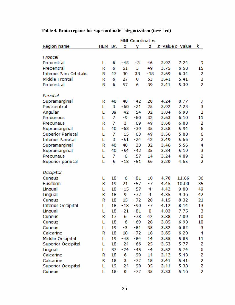
Table 3 (intact sounds) and Table 4 (inverted sounds) list brain regions that
participated in superordinate categorization. Figure 11 shows the group result of
searchlight analysis between animate and inanimate sound categories for intact (top) and
inverted (bottom) sounds. On the temporal lobes, the searchlight revealed far more voxels
for intact sound categorization (total number of voxel clusters: 1064) than for inverted
sound categorization (total number of voxel clusters: 562). The intact animate vs.
inanimate sound categorization yielded a large cluster of voxels that extend along the
superior temporal sulcus (STS) and gyrus (STG) whereas inverted animate vs. inanimate
sound categorization yielded several small clusters in the superior temporal lobes.
Additionally, extensive extra-temporal regions were found to participate in superordinate
categorization for both conditions (Tables 3 & 4). More voxels were found in the
occipital visual cortex for inverted sound categorization (total number of occipital voxels:
253) than for intact sound categorization (total number of occipital voxels: 26). In the
frontal lobe, superior frontal and precentral regions elicited different neural patterns
between animate and inanimate sound categories for both conditions. In the parietal lobe,

!"#
the superior and inferior parietal lobule, supramarginal gyrus, precuneus, and postcentral
gyrus generated categorical neural patterns between animate and inanimate sounds for
both conditions.
Figure 10. Sound object identification results at the superordinate level for intact
and inverted sounds While subjects were significantly worse at recognizing inverted
sounds than intact sounds, mean accuracy (65%) of inverted sound category identification
was significantly above the chance level (50%), indicating that subjects were reliably
able to recognize those inverted sounds at the superordinate level.

!!"
Figure 11. Brain regions participating in superordinate categorization for both
intact and inverted sounds For the intact sounds, a large number of voxel clusters were
found to distinguish between animate and inanimate sound categories. For the inverted
sounds, several smaller voxel clusters were found to distinguish between animate and
inanimate sound categories throughout the superior and middle temporal areas. More
voxels appear near the occipito-temporal junction and occipital lobes for the inverted
sound conditions. It is conceivable that subjects may have engaged visual processing to
make sense of those inverted sounds.

!"#
Table 3. Brain regions for superordinate level categorization (intact sounds)
!"#
Table 4. Brain regions for superordinate categorization (inverted)

!"#
fMRI (GLM)
All sounds vs. baseline: Both intact and inverted sounds yielded activation in the
similar brain regions regardless of the degree of recognizability (see Figure 12 top and
bottom). For instance, all the animate and inanimate sounds activated a large expanse of
auditory cortices bilaterally. Additionally, the sounds activated frontal regions as well as
bilateral precentral gyrus (p<0.05 (FDR), extent cluster size=2).
Animate vs. Inanimate (intact sound): Animate-inanimate subtraction yielded
activation mostly in the bilateral auditory cortices. By contrast, inanimate-animate
subtraction yielded few voxels in two white matter regions (p< 0.005 (uncorrected),

!"#
extent cluster size=10) (see Figure 13).
Animate vs. Inanimate (inverted sound): Similarly, animate categories of inverted
sound also activated mostly the bilateral auditory cortices but inanimate categories
yielded few white matter voxels (p< 0.005 (uncorrected), extent cluster size=10) (see
Figure 14).
#
!"#$%&' ()*' +,&' #%-$.' %&/$01/' -2' 345' /,-6"7#' 1,&' 8%&8/' 1,81' 6&%&' 9-%&'
8:1";81&<'=>'800'1,&'/-$7</'?87"981&'@'"787"981&A'1,87'=>'=8/&0"7&*#$%&#'()*+'#
,-./0,.&+#,#1,23&#&45,*'&#(6#7/1,.&2,1#,)+/.(28#-(2./-&'9#52&-&*.2,1#382/9#,*+#/*6&2/(2#
62(*.,1#,2&,':##
#

!"#
#
!"#$%&' ()*' +,&' #%-$.' %&/$01/' -2' 345' 6-7.8%"9#' 89"781&' 89:' "989"781&'
681&#-%"&/'-2'"91861'/-$9:/#$%&'()*#+#,%(%&'()*#-./)0(1)&2%#3&*45*5#(#4(06*#14.-)*0#
27#829*4-#2%# ):*#/&4()*0(4# -.;*0&20# )*';20(4# 0*6&2%-#<:*0*(-# ,%(%&'()*# +#$%&'()*#
-./)0(1)&2%#3&*45*5#(#7*<#-'(44#829*4#14.-)*0-#&%#<:&)*#'())*0=##
#
#

!"#
!
"#$%&'! ()*! +,'! $&-%.! &'/%01/! -2! 345! 6-7.8	$! 89#781'! 89:! #989#781'!
681'$-&#'/! -2! #9;'&1':! /-%9:/# $%&'()*# +# ,%(%&'()*# -./)0(1)&2%# 3&*45*5# (# 4(06*#
14.-)*0# 27# 829*4-# 2%# ):*# /&4()*0(4# -.;*0&20# )*';20(4# 0*6&2%-# <:*0*(-# ,%(%&'()*# +#
$%&'()*#-./)0(1)&2%#3&*45*5#(#7*<#-'(44#829*4#14.-)*0-#&%#<:&)*#'())*0=##
#
#
<#/6%///#-9!#
#
!"#$%&"'($)%*&+$*,$%(-$*.&+$//'"'%,&*)-%+&0#,'()"$'*&#,&#&*1'0$/$0&2'3'2&&
In this study, we sought to examine the neural basis underlying environmental
sound categorization. In particular, the present study hypothesized that there exist level-
specific auditory categorization areas that produce differential neural responses to
distinguish different categories in their own categorization levels. To address this
question, we performed a searchlight analysis at the following three levels:
i) Between animate and inanimate categories (superordinate level categorization)
ii) Among different animate categories (basic level categorization)
iii) Among different inanimate categories (basic level categorization)

!"#
Our findings revealed that a large expanse of bilateral auditory cortices
distinguish between animate and inanimate sound categories with differential neural
responses. In the superior temporal region, the anterior superior temporal sulcus robustly
produced differential neural patterns between animate and inanimate sound categories.
Importantly, this area has been implicated as an environmental sound processing region
(Zatorre et al., 2004). The converging neurophysiological and anatomical evidence
suggests that the antero-lateral superior temporal stream may be involved in auditory
object processing- the auditory “what” pathway (Hackett et al., 1999; Rao et al., 1997;
Rauschecker, 1998; Romanski et al., 1999)
The searchlight at the basic-level (within animate & within inanimate) also
revealed many voxels in classical auditory areas. This stands in stark contrast with the
previous finding by Lewis et al. (2005) demonstrating that a small locus on the middle
superior temporal gyrus was more activated by animate sounds than by inanimate sounds.
They, however, did not find any superior temporal regions that were more activated by
inanimate sounds. Similarly, our complementary GLM analysis (animate - inanimate)
yielded activation in a large cluster of bilateral superior temporal regions (see Figure 13
& 14) for both intact and inverted sound conditions. However, the reverse subtraction of
(inanimate - animate) for both condtions yielded only a small number of white matter
voxels. These traditional GLM analyses appear to suggest that auditory cortex is
inherently sensitive to the acoustic characteristic of animate sounds, but not inanimate
ones.
However, our MVPA results suggest a different story. There clearly exist
different subsets of voxels that are discriminative of either animate sounds or inanimate

!"#
sounds (Figure 9). Notably, the voxels that emerged for within animate and inanimate
categories were separated along a medial-lateral line resembling the animate vs.
inanimate spatial segregation within the ventral visual cortex (Chao et al., 1999; Grill-
Spector, 2003; Downing et al., 2006; also see Martin, 2006 for review). This is the first
observation in the auditory domain that reveals a lateral-to-medial organization between
auditory and visual regions for animate and inanimate categorization.
In all three analyses, several regions were also found that distinguished between
auditory categories in addition to the auditory cortex. While the average voxel cluster
sizes of those areas is smaller than those of dedicated auditory temporal regions, t-values
indicating separability of those voxels were high. One possibility is that those areas might
be able to distinguish animate vs. inanimate categories independent of modality. This led
to the follow-up audio-visual experiment described below.
The role of inverted sound
Initially, the inverted sound condition was designed to serve as a control condition
in order to tease apart high level from low level areas. Animate and inanimate categories
of sounds are different not only at the conceptual level, but also at the low level (e.g.,
acoustic structure). Therefore, a control was needed that equated for feature properties in
order to ensure any identified areas were specific to the conceptual differences not low
level acoustic features. By comparing intact and inverted sound results, we expected to
better identify the role of regions that would be found.
However, the inverted sound turned out to be still recognizable at the superordinate
level (Figure 10). This could be due to the temporal pattern of the acoustic properties. For

!"#
instance, animate sounds tend to be temporally irregular (e.g., horse whinny) whereas
inanimate sounds tend to be temporally regular (helicopter rotors). This was an
unexpected outcome; nevertheless the inverted sounds brought up some intriguing
findings due to their unique aspect of level-specific recognizability. Behavioral testing
showed that unlike the intact sounds, which were all recognizable both at superordinate
and basic-level, inverted sounds were only recognizable at the superordinate level. The
difference between superordinate and basic-level performance can be directly related to
the fMRI results at both superordinate and basic levels. The searchlight analysis revealed
many voxels throughout the brain including in classical auditory cortex for the
superordinate comparison (animate vs. inanimate). Intriguingly, far more voxels were
found in visual cortex for the inverted sound condition than for the intact sound
condition. It is plausible that subjects may have engaged in visual mental imagery to
make sense of those inverted sounds. Overall, both intact and inverted sounds at the
superordinate level yielded a large number of voxels.
By contrast, the searchlight did not yield any voxels at the basic-level (Figure 8) for
the inverted sounds. This result corresponds with the poor behavioral results seen for
basic-level categorization of inverted sounds. This supports the hypothesis that
categorization at a specific level can be achieved by eliciting differential neural patterns.
It is reasonable to conclude that the failure of identifying inverted sounds comes from
indistinguishable differential neural patterns on those sounds within the areas that were
identified in the intact condition.
!"#
Experiment 2
Multi-modal brain regions for object categorization

!!"
Introduction
Findings in the first study implicated a number of brain regions far downstream
from early auditory cortex in sound categorization. This naturally raises the following
question: “Are those non-temporal areas involved in categorization processing
independent of modality?” If that is the case, we should be able to identify the same
regions using visual stimuli as well. The second study explores that possibility.
Materials and methods
Subjects
Eleven healthy volunteers (average age: 27.1, 5 females) participated in this
study. None of the volunteers had hearing difficulties or neurological disorders. Consent
forms were received from all subjects as approved by the Human Subjects Institutional
Review Board of Dartmouth College.
Stimuli
Auditory stimuli: Twelve different environmental sounds (6 animate & 6
inanimate sounds) were obtained from a commercial sound effect library (Hollywood
Edge, The Hollywood Edge, USA). Animate sounds included exemplars of: human
coughing, cat mewing, dog barking, horse whinnying, cow mooing, and pig oinking
sounds. The inanimate sound category included exemplars of: car engine, phone ring,
alarm clock, helicopter rotor, airplane engine, and camera shutter sounds. All the stimuli

!"#
were matched in duration (~ 2sec), sampling rate (44.1 kHz, 16-bit, stereo) and root mean
squared power, and an envelope of 20 ms was applied to avoid a sudden clicking sound at
onset and offset using a sound editing software (Sound Forge 9.0, Sony, Japan). Stimuli
were delivered binaurally using a high-fidelity MR-compatible headphone (OPTIME 1,
MR confon, Germany) in the scanner.
Visual stimuli: Forty-eight different high quality photographic pictures (24
animate & 24 inanimate images) were obtained from Google image search engine
services ($%%&'(()*+,-./,00,1-/20*). Six animate (human, cat, dog, horse, cow, and
pig) and 6 inanimate image categories (car, phone, clock, airplane, camera, and
helicopter) were used. Four exemplars were included in each category (e.g., human 1,
human 2, human 3, and human 4). Objects in the images were carefully cut out from
their backgrounds using a Photoshop plugin ($%%&'((333/4),)%+15)1*%001./#
20*(-6*+.7() and placed onto identical gray backgrounds. The RGB intensity was
normalized across all the images. The exemplars were then converted to 2-seccond video
file format (.avi) using Adobe Premiere Pro CS3 (333/8409-/20*(:;-*)-;-# :;0()
and Xvid Codec compression (333/<=)4/0;,().
fMRI scanning
fMRI scanning was conducted on a Philips Intera 3T whole body scanner. (Philips
Medical System, Best, The Netherlands) at the Dartmouth College Brain Imaging Center.
Parameters of the standard echo-planar imaging were: TR= 2000 ms, TE= 35 ms, FOV=
240 x 240 mm, 30 slices, voxel size =3 x 3 x 4 mm, inter-slice interval =0.5 mm,

!"#
sequential axial acquisition. Subjects completed 4 functional runs (244 TRs) for each
auditory and visual condition, which were acquired on different days. Either one HIRES
MPRAGE scan or one DTI scan was additionally acquired at the end of each scan
session.
Experimental procedures
i) Auditory condition
During functional imaging, subjects performed 6 iterations of an auditory memory
task while maintaining visual fixation. In each iteration of the task, subjects heard a series
of 8 auditory stimuli, separated by an 8 second delay. These stimuli were randomly
selected from among the 6 animate and 6 inanimate sound categories. Exemplars were
not repeated within a task iteration. After the 8th stimulus, the fixation cross was changed
to the following instruction: “Was this sound previously presented during the task
session?” while a 9th stimulus was concurrently played. Half of the time, the last stimulus
was identical to one of the 8 presented stimuli; half of the time it came from an
uninterested category (e.g., duck, elephant, etc). Subjects indicated whether or not the
probe stimulus matched a presented stimulus by pressing a button, ending the task
iteration. There was an 8 second rest period before the next iteration of the task began.
ii) Visual condition
During each run, subjects viewed a series of 4 images from one category (e.g.,
human 1, human 2, human 3, human 4), each presented for 500 ms (total 2 sec. ). A new
series appeared every 8 sec. The order of the 4 images within a series was randomized.

!"#
On some trials, an oddball stimulus would appear: one of the images in the series would
be from a different category. Subjects indicated the detection of an oddball by pressing a
button. Ten percent of the total number of stimuli presented were oddballs.
fMRI data analysis methods
fMRI data was preprocessed using the SPM5 software package (Institute of
Neurology, London, UK) and MATLAB 2008a (Mathworks Inc, Natick, MA, USA). For
multivariate fMRI analysis, all images were realigned to the first EPI to correct
movement artifacts, and spatially normalized into Montreal Neurological Institute (MNI)
standard stereotactic space (e.g., ICBM152 EPI template) with preserved original voxel
size (3 mm x 3 mm x 4 mm). For univariate fMRI analysis, a separate copy of the same
data was spatially smoothed (8-mm full width half maximum Gaussian).
Univariate fMRI analysis: After image preprocessing was completed, each run
was submitted to the general linear modeling to estimate the regression coefficient of all
the conditions. For the modeling, the onset of each condition (e.g., all the sounds &
button presses) was convolved with the canonical hemodynamic response function. 6
motion parameters were later regressed out as nuisance variables. In order to create the
contrast map between animate and inanimate categories, each condition was assigned to
‘1’ or ‘-1’ depending on the direction of subtraction analysis (e.g., for animate -
inanimate subtraction, ‘dog’ condition was assigned with ‘1’ and ‘car’ condition was
assigned with ‘-1’ and vice versa). The resulting contrast image of each subject’s data

!"#
was in turn passed on to the 2nd
level random effect analysis to generate a t-map of
across-subject effects.
Multivariate fMRI analysis: We used the “searchlight” technique developed by
Kriegeskorte et al. (2006). The key characteristic of the searchlight technique is the
movement of a searchlight sphere through entire brain, performing a classification test
using a machine learning classifier at each location (for more details, see Kriegeskorte et
al., 2006). We used a searchlight consisting of a discrete sphere with a radius spanning
two voxels distant from a center voxel.
Classification between animate and inanimate categories: fMRI time-courses of
all voxels were extracted from unsmoothed images. These raw signals were then high-
pass filtered with a 300s cut-off to remove scanner-caused slow signal drifts in signal and
standardized across entire runs to normalize intensity differences between the runs.
Signals corresponding to the time-points of each condition (i.e., images acquired at 3
consecutive TRs; 4 second after the onset of stimulus) were acquired from voxels
belonging to each searching unit. Based on the canonical hemodynamic function
modeling, the signals acquired from those three time points were not mixed with those
driven by other category of sound. Next, responses to the 6 animate and 6 inanimate
categories of images or sounds were collapsed to form an “animate” class and an
“inanimate” class. These data were converted to a vectorized format to be fed into a
classifier. We used a Lagrangian Support Vector Machine (Mangasarian & Musicant,
2001). The classifier was initially trained on one strict subset of the data (a training set)

!"#
then tested on the remaining data (a test set). For the purpose of validating results, signals
of 3 scanning runs served as a training set and 1 run served as a testing set in turn,
resulting in 4-fold cross validation in each auditory and visual condition (see the
introduction for the general concept and procedure; see also the tutorial review on MVPA
by Pereira et al. (2009)). The percent correct result per each searchlight sphere was
averaged across 4 folds and stored in every voxel of an output image for each subject.
The output images of all subjects were passed into a second-level random effect analysis
(Raizada et al., 2009; Walther et al., 2009; Stokes et al., 2009) using SPM5 to generate a
group map where each voxel was assigned a corresponding t-value that indicates the
degree of separability between animate and inanimate visual or auditory category in the
location.
Audio-visual area identification: After performing the searchlight analysis for
auditory and visual condition separately, all the significant voxels (the center voxels of
searchlight spheres) were listed in tables. To identify the brain regions that contain both
auditory and visual responses, we referred to the AAL (Automated Anatomical Labeling)
map that is built-in in MRIcron software (http://www.cabiatl.com/mricro/mricron/). The
inter-cluster distance was calculated on all the pair-wise combinations (e.g., if two
auditory clusters and two visual clusters were found within the same anatomical areas,
total number of pair-wise distance would be 4.)

!"#
Results
Tables 5, 6, and 7 list brain regions that were found to distinguish between
animate and inanimate categories in the visual, auditory, and audio-visual domain
respectively.
fMRI(MVPA)
Auditory categorization areas: The whole-brain searchlight revealed a sizable
cluster of voxels in the bilateral temporal lobes as well as several extra-temporal regions
that generated differential neural response pattern between animate and inanimate sounds
(p< 0.05 (FDR) 2)(see Figure 15, & Table 5). These non-temporal regions include middle
frontal gyrus, inferior frontal gyrus, supplementary motor area, precentral gyrus on the
frontal lobe; superior and inferior parietal lobule, angular gyrus, supramarginal gyrus,
post central gyrus, and precuneus on the parietal lobe; superior and middle occipital
gyrus, and calcarine sulcus on the occipital lobe. These findings are consistent with the
findings of experiment 1 using different sets of animate and inanimate sound categories,
therefore they confirm our previous findings (see Table 3 & 4).
Visual categorization areas: The whole-brain searchlight revealed that a large
expanse of occipital and inferior temporal lobes distinguished between animate and
inanimate categories (p< 0.05 (FDR)) (Figure 15). Additionally, several regions beyond
the visual cortex that were able to distinguish between animate and inanimate images

!"#
were found, including frontal, parietal, temporal, cerebellar, and subcortical areas such as
the hippocampus, and the thalamus (Table 6).
Audio-Visual categorization areas: Table 7 lists brain regions and intercluster
distances between auditory and visual loci within the same anatomical regions. Figure 16
shows representative audio-visual categorization areas with small intercluster distances.
These audio-visual areas include superior medial frontal gyrus, inferior frontal gyrus,
precentral gyrus, and supplementary motor area in the frontal lobe; superior parietal
lobule and precuneus in the parietal lobule; middle and superior occipital regions; the
posterior portion of superior and middle temporal regions; and the fusiform and insula on
the temporal lobe. The intercluster distance varies between regions. Based on the radius
of the searchlight sphere (7.5 mm), we set an arbitrary criterion was set for “overlapping”
regions at 15 mm (the maximum distance spanned by two abutting searchlight spheres).
Several regions meet the criterion: supplementary motor area (0 mm; 11.53 mm) and
precentral gyrus (4 mm), superior parietal lobule (11.22 mm), superior occipital gyrus
(9.49 mm), and fusiform gyrus (13.42 mm). Interestingly, in the supplementary motor
area, the same coordinate corresponds to both auditory and visual clusters (MNI: 3, 9,
63).

!"#
Figure 15. The lateral view of brain areas that distinguish between animate and
inanimate categories in each modality While most voxels for visual and auditory
categorization are in classically unimodal early sensory areas, voxels in other regions also
appear for both modalities. This suggests that these areas may be able to distinguish
between animate and inanimate categories in a supramodal manner.

!"#
Figure 16. Representative brain regions containing auditory and visual responses
The blue cross-hair pin-points the center voxel of the searchlight sphere. It can be seen
that auditory and visual cluster are centered on the exactly same coordinate on the SMA.
Both pSTS and fusiform that are known as a classical “animacy” detecting regions also
appear in this analysis.

!"#
Table 5. Brain regions distinguishing animate vs. inanimate categories (visual)

!!"
Table 6. Brain regions distinguishing animate vs. inanimate categories (auditory)

!"#
Table 7. Brain regions that were found in both auditory and visual categorization
fMRI (GLM)
Auditory vs. Visual comparison: The subtraction of auditory- visual maps yielded
activation mostly within auditory cortices bilaterally. Likewise, the subtraction of [visual
- auditory] yielded activation mostly within visual cortex (p<0.05 (FDR), extent cluster
size=2) (Figure 17).

!"#
Animate vs. Inanimate (visual): Overall, the brain areas seen in this comparison
were more activated by animate categories than inanimate categories of images (p<0.005
(uncorrected), extent cluster size=10). Notably, the lateral portion of the ventral temporal
lobe was more activated by animate categories whereas the medial portion of the ventral
temporal lobe was more activated by inanimate categories (Figure 18). This result is
consistent with previous findings (Chao et al., 1999; Grill-Spector, 2003; Downing et al.,
2006; also see Martin, 2006 for review)..
Animate vs. Inanimate (auditory): The bilateral auditory cortices were more
activated by animate sounds than by inanimate sounds. No voxel was found to be more
activated by inanimate sounds at the threshold used (p<0.005 (uncorrected), extent cluster
size=10) (Figure 19).

!"#
Figure 17. Group map of GLM results showing the areas that were more activated
by auditory stimuli than by visual stimuli and vice versa. Each sound and image
activated its classical early sensory areas (e.g., temporal region for sound and occipital
and ventral temporal areas for images).

!"#
Figure 18. Group map of GLM results comparing animate vs. inanimate categories
of images Overall, animate images activated more brain areas than inanimate categories.
It can be seen that the lateral ventral temporal lobe is more activated by animate
categories of images whereas the medial ventral temporal lobe is more activated by
inanimate categories of images. This result is consistent with previous reports.

!"#
Figure 19. Group map of GLM results comparing animate vs. inanimate categories
of sounds It can be seen that activation mostly occurred in the bilateral auditory cortices
by animate sounds. By contrast, no voxels were found to be more activated by inanimate
sounds than by animate sounds (p<0.005 (uncorrected), extent cluster size=10).
Discussion
This audio-visual experiment sought to address the following two questions:
- Are brain regions far downstream from the early sensory cortex able to distinguish
between animate and inanimate categories in a supramodal manner?
- If so, does the same set of voxels within a region respond to both auditory and visual
sensory input, or is a distinct subset of voxels exclusively dedicated to either the auditory
or visual modality?
!"#
Using a searchlight analysis, we identified several areas that produced differential
neural patterns for animate and inanimate categories of images as well as sounds (Figure
16 & Table 7) beyond the early sensory stations of auditory and visual modality.
The distance was then measured between the center voxel of auditory and visual
cluster within the same region (Figure 16). The distance varies across different regions
(0-38.5 mm): in some areas, auditory and visual clusters are located within a putatively
overlapping region (within 15 mm) (e.g., in the right supplementary motor area, the
distance between auditory and one of the visual clusters is 0). Given the distance, it is
quite feasible that this region may be involved in animate vs. inanimate distinction
independent of modality. Further research attempts with methods such as non-human
primate electrophysiology should be made to evaluate this conjecture.
Early vs. late sensory areas for modality specific and independent processing
Our results revealed both early and late sensory areas in each modality. As can be
seen in Figure 15, most voxels were found within classical early sensory areas for both
auditory and visual processing. Within those early areas, no voxels were found to co-
occur for animate vs. inanimate categorization of both modalities. However, auditory and
visual responses were found in several brain regions beyond the early auditory and visual
cortex. Some of those areas have been implicated in studies looking at high level
conceptual processing such as “animacy” or “tool-use” detection (Wheatley et al., 2007;
Frey et al., 2005). Thus, we speculate that the identified areas in this study may serve to
readily recognize whether or not the received sensory cue is from a living or artificial

!"#
source, regardless of sensory modalities. Further research should better identify the role
of each of those areas and their multimodal characteristics.
Together, the findings of this study suggest that incoming sensory signals may be
processed in two steps: 1) in a modality-specific manner within the early sensory cortex
(e.g., individual feature extraction of visual and auditory frequencies) 2) in a modality-
independent manner within the late sensory areas (e.g., understanding the concept of the
object).
Modality dependent task design
In this study, we employed different strategies for the auditory and visual
conditions to elicit subject’s attention: in the auditory condition, a memory task was
given to subjects, but an oddball task was given in the visual condition. As described in
the method section, four images from the same category were presented in each trial
during the visual condition but not the auditory condition. We implemented the four-
image sequence after failing to acquire a good fMRI signal from the visual condition
when we presented only one image per each trial and employed the same memory task as
in the auditory condition. The visual cortex appeared to be quickly adapted by a long
exposure to one image and the memory task appeared to be accordingly ineffective.
During the second data collection period, we instead presented multiple images briefly
(500 ms per each image, totaling 2 seconds per trial) and employed the oddball task in
order to ensure that subjects attended to the each of the clustered pictures.
Although the tasks were different between conditions, we conjecture that this did
not affect the measured fMRI activity to reflect each category of object. The quality data

!"#
acquired using the new experimental design for visual stimuli substantially improved,
such that we did not observe any habituation effect in the visual cortex.
#
!"#
Chapter 3.
Neural bases of melodic contour categorization
#
#
#
#
#
#

!"#
Introduction
#
#When listening to music, we effortlessly follow a series of ups and downs
between notes in a melody. While this ability appears to be hard-wired (Trehub et al.,
1987; Plantinga & Trainor, 2005; Volkova et al., 2006), about 4% of the population is
born with deficits in melodic processing, a disorder called “amusia” (Ayotte et al., 2002;
Peretz & Hyde, 2003), This impairment can also be also acquired by brain damage; for
example, Johnsrude et al. (2000) showed that patients with a lesion in the right superior
temporal lobe were not able to judge the direction of pitch change (e.g., rise/fall) of a
two-note melody, despite reliably discriminating whether the notes were the same or
different. This partial impairment clearly suggests that pitch discrimination and pitch
contour recognition are independently processed. Warrier et al. (2008) also showed that
patients with a right temporal lobe lesion did not benefit as much as control subjects –
patients with a left temporal lobe lesion – from melodic context when performing a pitch
constancy task2. Further evidence supporting the notion of the right superior temporal
region as the hub of a melodic processing center has been provided by several
neuroimaging studies (Zatorre et al., 1994; Johnsrude et al., 2000; Warrier et al., 2004;
Hyde et al., 2008; Stewart et al., 2008). In an early PET imaging study, Zatorre et al.
(1994) showed that the right superior temporal sulcus was more activated when listening
to a melody than during a noise burst. More recently, Hyde et al. (2008) showed that the
right superior temporal region was parametrically modulated by the degree of pitch
########################################################2 Pitch constancy task: judge whether the fundamental frequency is the same or different
for tones with different spectral range (e.g., A4 (F0=440 Hz) of piano and guitar)

!!"
distance in melodic sequences whereas the left superior temporal region was not
responsive until the pitch distance was increased to 200 cent between adjacent notes.
Together, these studies suggest that the right superior temporal region is specialized for
melodic processing.
The present study seeks to identify the neural basis of melodic processing; in
particular, the study tests the hypothesis that melodic contour may be categorically
represented. More specifically, we hypothesize that the categorical representation of
melodic contour is achieved through differential neural patterns. While the right superior
temporal region is a strong candidate to show categorical neural response related to
melodic contour, we also sought to identify other areas that can distinguish between
ascending and descending melodies using such a strategy.
Could melodic contour be one of the most critical components to understanding
melodies? Several behavioral studies have shown that melodic contour provides an
essential basis for characterizing a particular melody (Dowling & Fujitani, 1971;
Dowling, 1978; Barlett & Dowling, 1980; Dowling et al., 1987; for review, see Dowling,
1994). For instance, Dowling & Fujitani (1971) showed that contour influenced the
recognition of transposed melodies such that melodies with subtle differences in their
consisting notes but that were preserved with the same contour tended to be perceived as
identical when transposed. In another study, Dowling et al. (1987) showed that subjects
were worse at detecting a subtle change of pitch sequence between melodies with the
same contour than for melody pairs with different contours.
This study is the first to examine the neural basis of such melodic contour
processing. We identified three brain regions that robustly distinguished between

!"#
ascending and descending melodies through comparable though differential neural
patterns: right superior temporal sulcus (STS), left inferior parietal lobule (IPL), and
anterior cingulate cortex (ACC). Our further control analysis on the major vs. minor
distinction showed that those areas may distinguish different melodies based on their
structure, but not on their emotional content. Furthermore, the multidimensional scaling
analysis on the similarity distance among all the melodies revealed that subjects
perceptually found melodies with the same contour more similar than melodies with a
different contour, supporting the notion of categorical representation of ascending and
descending melodies.
Materials and methods
Subjects
Subjects were 12 healthy right-handed volunteers (7 male; average age = 20.4;
average musical training = 5.7 years), none of whom majored in music nor had
participated in professional or semi-professional music activities (e.g., playing in an
orchestra or a rock band). No subjects had absolute pitch. Consent forms were obtained
from all subjects as approved by the Committee for the Protection of Human Subjects at
Dartmouth College.
Stimuli
Twenty short melodic sequences consisting of five piano tones in the middle
octave range were generated using the MIDI sequence tool in Apple’s GarageBand

!"#
software and exported to .wav format (Figure 20). All stimuli were matched in duration
(2.5 sec) and sampling rate (44.1 kHz, 16-bit, Stereo) using SoundForge 9.0 (Sony,
Japan). Root mean square (RMS) power was adjusted across all the stimuli using an in-
house Matlab script. A 2x2 design was employed with Mode (major, minor) in one
dimension and Melodic Contour (ascending, descending) in another dimension, creating
four categories of stimuli, each of which contained five different types of scales (Figure
20). In addition to these 20 stimuli, four oddball melodies consisting of both ups and
downs of pitch changes were created (see figure 40 in the appendix).
Figure 20. Staff view of the 20 melodies generated using MIDI software
a. Diatonic scale, b. 7th
scale, c. Arpeggio scale, d. 5th
scale, e. Wide arpeggio scale
All the melodies were chosen on the C key in the middle octave range.
The tempo of each melodic sequence was 120 bpm (duration of each melody is 2.5
sec).
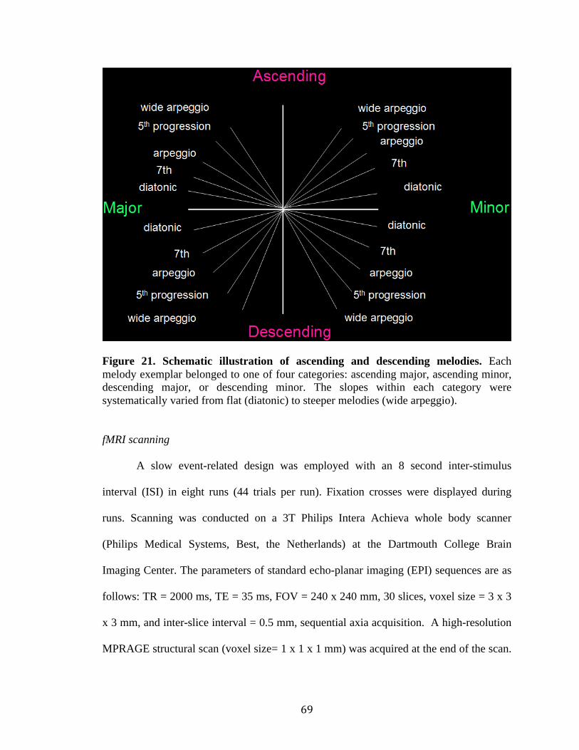
!"#
Figure 21. Schematic illustration of ascending and descending melodies. Each
melody exemplar belonged to one of four categories: ascending major, ascending minor,
descending major, or descending minor. The slopes within each category were
systematically varied from flat (diatonic) to steeper melodies (wide arpeggio).
fMRI scanning
A slow event-related design was employed with an 8 second inter-stimulus
interval (ISI) in eight runs (44 trials per run). Fixation crosses were displayed during
runs. Scanning was conducted on a 3T Philips Intera Achieva whole body scanner
(Philips Medical Systems, Best, the Netherlands) at the Dartmouth College Brain
Imaging Center. The parameters of standard echo-planar imaging (EPI) sequences are as
follows: TR = 2000 ms, TE = 35 ms, FOV = 240 x 240 mm, 30 slices, voxel size = 3 x 3
x 3 mm, and inter-slice interval = 0.5 mm, sequential axia acquisition. A high-resolution
MPRAGE structural scan (voxel size= 1 x 1 x 1 mm) was acquired at the end of the scan.

!"#
Stimuli were delivered binaurally using high-fidelity MR-compatible headphones
(OPTIME 1, MR confon, Germany).
Experimental Procedures
i) fMRI experiment
During the scan, subjects heard a series of ascending and descending contours (Figure
20). For the task, subjects were asked to press a button to indicate melodies that consisted
of both ups and downs of pitch contour (see figure 40 in the appendix).
ii) Happiness rating
Subjects were later brought to the laboratory. In a quiet behavioral testing room,
stimuli were presented with noise-canceling headphones (Quiet Comfort acoustic noise-
canceling headphones, Bose, U.S.A.) and participants reported their response to each
sequence using a Likert-type scale from 1 (very sad) to 7 (very happy).
iii) Similarity distance measurement
Also in the laboratory, subjects were presented with consecutive pairs of
sequences consisting of the stimuli from the fMRI study and asked to indicate how
similar each pair of melodies (400 pairs, 20x20) sounded using a Likert-type scale from 1
(not at all similar) to 7 (exactly alike). Subjects were encouraged to use the full scale and
to try to make the average rating equal to 4. The full list comprised the set of all possible
pairings, presented over the course of two half-hour sessions. Equipment used was the
same as in the other behavioral experiment.

!"#
MRI data analysis methods
fMRI data was preprocessed using the SPM5 software package (Institute of
Neurology, London, UK) and MATLAB 2009b (Mathworks Inc, Natick, MA, USA). For
multivariate fMRI analysis, all images were realigned to the first EPI to correct
movement artifacts, and then spatially normalized into Montreal Neurological Institute
(MNI) standard stereotactic space (e.g., ICBM152 EPI template) with its preserved
original voxel size (3 mm x 3 mm x 3 mm). For univariate analysis, a separate copy of
the same data was spatially smoothed (8-mm full width at half-maximum Gaussian) after
the normalization.
Univariate fMRI analysis: After image preprocessing including the smoothing
step was completed, each run was submitted to the general linear modeling to estimate
the regression coefficient of all the conditions. For the modeling, the onset of each
condition (e.g., all the sounds & button presses) was convolved with the canonical
hemodynamic response function and six motion parameters were integrated to be later
regressed out as nuisance variables. In order to create the contrast map between
ascending and descending melody categories, each ascending and descending melody
was assigned with ‘1’ or ‘-1’ depending on the direction of subtraction analysis. The
resulting contrast image of each subject’s data was, in turn, submitted to the 2nd
level
random effect analysis to generate the group resulting map (p(uncorrected) < 0.005,
extent voxel cluster size=10) .

!"#
Multivariate fMRI analysis: We used the searchlight technique developed by
Kriegeskorte et al. (2006). The key concept of the searchlight technique is to move a
spherical searchlight sphere through the brain and perform a classification test using a
machine-learning classifier at each location (for more details, see Kriegeskorte et al.,
2006). We chose a radius size consisting of two neighboring voxels from the center
voxel.
Classification between ascending and descending melodies: fMRI time-courses
of all voxels were extracted from unsmoothed images. Subsequently, these raw signals
were high-pass filtered with a 300s cutoff to remove slow drifts caused by the scanner,
and standardized across entire runs to normalize intensity differences among runs. In
order to avoid confounding signal from different stimulus onsets, signal solely generated
by each stimulus (i.e., corresponding to time points 4, 6, and 8 seconds after the onset of
the stimulus) was acquired from voxels belonging to each searching unit. The stimuli
belonging to each category were converted to the proper format to be used as activation
vectors for each condition, which were then passed into a classifier. For the binary
classifier, we used the Lagrangian Support Vector Machine algorithm (Mangasarian &
Musicant, 2001). The classifier was initially trained by a strict subset of datasets (training
set) and applied to the remaining datasets (testing set). For the purpose of validating
results, signals from six scanning runs served as a training set and two runs served as a
testing set, resulting in 4-fold cross-validation. The percent correct result for each
searchlight sphere was averaged across the four training/testing combinations and stored
in each voxel of an output image for each subject. These output images of all subjects

!"#
were submitted to a second-level random effect analysis (Raizada et al., 2009; Walther et
al., 2009; Stokes et al., 2009) using SPM such that the average accuracy of classification
test for each voxel was compared to chance (50%) and the group t-map containing the
corresponding t-value for each voxel was generated.
!
Results
Behavioral results (happiness rating)
A one-way repeated ANOVA was performed on the average happiness ratings
across the four melodic categories. The results revealed that there was a significant
difference among the four categories, F[3,33] = 19.99, p < 0.05 (Figure 22). Also, there
was a main effect of contour such that ascending melodies sounded happier than
descending melodies irrespective of mode, t(11) = 5.58, p < 0.05 (Figure 23). Likewise,
there was a main effect of mode such that major melodies sounded happier than minor
melodies irrespective of contour, t(11)= 4.90, p < 0.05 (Figure 24). For the post-hoc t-test
on each pairwise comparison, see the appendix table 10.

!"#
Figure 22. Happiness ratings for the four melody categories. The x-axis depicts 4
different melodic categories and the y-axis is for the Likert scale between 1 and 7. There
was significant difference among the four melodies for its emotional content.
Figure 23. Happiness ratings for ascending and descending melodies. The x-axis
depicts ascending and descending melodies and the y-axis shows mean happiness ratings.
The bar graph indicates that ascending melodies sound happier than descending melodies.

!"#
Figure 24. Happiness ratings for major and minor melodies. The x-axis depicts major
and minor melodies and the y-axis depicts mean happiness ratings. The bar graph
indicates that major melodies sound happier than minor melodies.
Behavioral results (similarity distance matrix)
Similarity data were acquired from 7 out of 12 subjects who had participated in
the fMRI experiment, compiled in a square symmetrical matrix format, and analyzed with
SPSS v. 17.0 (Chicago, IL), generating 2-dimensional Euclidean-distance plots both
within and across subjects with S-stress convergence of .001. The multi-dimensional
scaling (MDS) structure indicated that the primary dimensions of clustering among the
sequences were binary by contour (ascending vs. descending) and continuous by slope
(steep to flat) (Figure 25). These results suggest that the contour is categorically
perceived by the human subjects such that melodies within the same contour tend to be

!"#
rated as more similar than melodies across different contours, regardless of the distance
between the slopes of melodies (e.g., ascending diatonic is rated as more similar to
ascending arpeggio than descending diatonic).
#
Figure 25. Multi-dimensional scaling structure on the similarity distance among all
pair-wise melody comparisons (total 2800 data points acquired from 7 subjects; 400
trials per each subject). The vertical axis captures the variance of the slopes and the
vertical axis captures the variance of the contour among the melodies. Because ascending
and descending is perceived categorically, contour may be one of the most crucial aspects
in melody perception.
fMRI (MVPA)
Ascending vs. Descending category: The searchlight analysis revealed three
distinct brain regions, namely right STS, left IPL, and ACC, that reliably categorized
between ascending and descending melodies (p(uncorrected) < 0.005, extent threshold =
10) (Figure 26). Among the areas, right STS (MNI x,y,z: 51,-18,-7) elicited the most
robust separability between the categories, t (11) = 7.71, confirming that melodic

!!"
processing is mainly mediated by the right superior temporal region (Zatorre, 1985;
Zatorre et al., 1994; Johnsrude et al., 2000; Warrier et al., 2004; Hyde et al., 2008).
Following rSTS, IPL (MNI x,y,z: -48, -36, 39) on the contralateral left hemisphere
showed categorical responses between the melodies. Within this region, the voxel with
local maxima of separability, t (11) = 5.59 lies on the intraparietal sulcus (Figure 26). On
the frontal lobe, local maxima of separability, t (11) = 4.66 was found in the ACC (MNI
x,y,z: 3, 21, 28). The voxel cluster size was anti-correlated with separability t-value such
that the biggest voxel clusters were found in the ACC and the smallest voxel clusters
were found in the rSTS (Table 8).
Major vs. Minor melodies category: Additionally, we also performed the whole
brain searchlight for the binary classification between major and minor melodic
categories. However, the searchlight of binary classification between major and minor
did not find significant areas that distinguished between major and minor melodies
(p(uncorrected) < 0.01, extent threshold =15). Thus, it is reasonable to conclude that
identified areas from the ascending vs. descending classification may be involved in
melodic contour categorization based on their different sequence structure, not emotional
content.

!"#
Figure 26. Brain regions that distinguish between ascending and descending melodic
sequences (p(uncorrected) < 0.005, extent cluster size=10) rSTS (top) generated the
most robust separable neural patterns between ascending and descending melodic
sequences (t (11) =7.71). Findings in rSTS are consistent with the current notion that this
region plays a central role in melodic processing. LIPL (middle) was the second best
categorizer between ascending and descending melodies (t (11) =5.59). The area has
recently received attention in the music fMRI field (Foster & Zatorre, 2010). ACC
(bottom) was also found to distinguish between ascending and descending melodies. The
area appears to monitor the dynamics in the melodic structure. See Figure 28 for the
GLM that compares melodies to baseline for further evidence.

!"#
Figure 27. The result of whole brain searchlight analysis between major and minor
melodies (p < 0.01, extent cluster size=15). No voxels were found that distinguished
between major vs. minor melodies, suggesting that the areas that we identified did not
show activation due to ascending melodies sounding happier than descending melodies.
Those three areas may categorically represent ascending and descending melodies based
upon the structure.
Table 8. Brain regions identified from MVPA and GLM analyses.

!"#
fMRI (Univariate GLM)
Melody vs. baseline: The subtraction of [all melodies – baseline] yielded a large
expanse of bilateral auditory cortices, premotor regions, and ACC (p(FDR) < 0.05, extent
cluster size=2) (Figure 28).
Ascending vs. Descending melodies: The subtraction of [ascending –
descending] did not yield any significant voxels in the gray matter (p(uncorrected) <
0.005, extent cluster size=10). However, the subtraction of [descending – ascending]
yielded sizable voxel clusters in the left superior frontal region (MNI x,y,z: 24, 45, 42)
(Figure 29; Table 8) .
Major vs. Minor melodies: The subtraction of [major - minor] yielded several
voxel clusters throughout the brain (p(uncorrected) < 0.005, extent cluster size=10).
These areas include superior and middle frontal gyrus in the frontal lobe; middle occipital
gyrus, precuneus, and posterior cingulate in the posterior lobe; and the anterior portion of
middle temporal sulcus in the temporal lobe (Figure 30; Table 8).

!"#
Figure 28. Group results of GLM showing areas more activated during melody
conditions than during rest (p(FDR) < 0.05, extent cluster size=2). Premotor areas as
well as ACC were more activated in addition to the large expanse of bilateral auditory
cortices, suggesting that these areas may be sensitive to the dynamics in the melody
structure.
Figure 29. Group result of GLM comparing ascending to descending melodies
(p(uncorrected) < 0.005, extent cluster size=10). The voxels that were more activated by
ascending melodies were situated on the white matter whereas the right frontal region
was found to be more activated by descending melodies.

!"#
Figure 30. Group result of GLM showing areas that were more activated by major
than minor melodies Whereas no voxels were found that were more activated by minor
melodies than by major melodies, several areas were found to be more activated by major
melodies than by minor melodies throughout the brain (p(uncorrected) < 0.005, extent
cluster size=10).
Discussion
This study sought to test the hypothesis that ascending and descending contours of
melodies are categorically represented by the brain through differential neural patterns.
Using a whole brain searchlight, we identified three distinct areas: rSTS, lIPL, and ACC
(Figure 26). The subsequent searchlight analysis on the mode (major vs. minor)
confirmed that these three areas likely distinguish melodies based upon the structure, not
based upon the emotional content of melodies (Figure 27). The similarity distance matrix

!"#
also revealed that the subjects tended to categorically perceive ascending and descending
melodies (Figure 25).
The role of rSTS
Consistent with the previous findings, rSTS was the best categorizer for ascending
vs. descending melodies among the areas that were identified (separability t (11) = 7.71) .
The center voxel of rSTS in our findings is approximately 15 mm from the area that was
previously found to be more activated by melodies than by noise in an early PET imaging
study (Zatorre at al.,1994). Given the large voxel resolution and smoothing in the early
PET study (5mm x 5mm x 6mm), it is quite plausible that these areas may be the same
neuronal population involved in melodic processing. With advanced neuroimaging
techniques in combination with a smaller voxel size (3mm x 3mm x 3mm), the current
MVPA study reveals that melodies are processed via differential neural patterns within
the rSTS.
It has been argued that the superior temporal region in each hemisphere is
specialized for processing different aspects of sounds such that the right superior
temporal region is involved in spatial processing (e.g., pitch distance) whereas the left
superior temporal region is involved in temporal processing (Griffiths et al., 2004; Hyde
et al., 2008; Peretz & Zatorre, 2005). This view was first proposed by lesion studies that
revealed a double dissociation between melodic and temporal processing (Milner, 1962;
Zatorre, 1985; Johnsrude et al., 2000). For example, Johnsrude et al. (2000) revealed that
patients with right temporal damage cannot discern the direction of two tones, even
though they can still discriminate between them. In another study, Di Pietro et al. (2004)

!"#
showed that a professional musician was not able to reproduce rhythmic patterns after
suffering left temporal lobe damage.
The advent of neuroimaging techniques has allowed the exploration of this
functional asymmetry between left and right auditory cortex with normal subjects (Hyde
et al., 2008; see review by Zatorre & Gandour, 2008). Hyde et al. (2008) revealed that the
right superior temporal region was modulated by the parametrical change of pitch
distance while the left superior temporal region was not responsive to subtle pitch
distance changes. Bengtsson & Ullen, (2006) reported that the left superior temporal lobe
was more activated by complex rhythmic structures than simple rhythmic structures.
Further, a number of studies have shown that the left superior temporal region plays a key
role for speech processing that requires temporal processing (Hickock & Poeppel, 2007).
Our finding is consistent with the prevailing notion of functional asymmetry
between left and right temporal lobes. In our study, there was no temporal difference
between ascending and descending melodies since they were matched for duration and
tempo. Thus, it is reasonable to attribute the findings in rSTS to the hemispheric
specialization in the processing of sounds. Further studies should examine the neural
basis of temporal processing mediated by the left superior temporal region.
The role of left IPL
It is well known that the parietal lobe is one of the key regions for the dorsal
visual ‘where’ pathway (Mishkin et al., 1983). While numerous studies have shown that
this area is activated by visual spatial tasks, the posterior parietal lobule is also known to
be involved in multi-modal processing (Schroeder & Foxe, 2002). A number of

!"#
neurophysiological studies have revealed that this area receives sensory inputs from
visual, auditory, and tactile sensory areas (see the review by Cohen, 2009). The parietal
lobe also appears to be involved in symbolic mapping, such as for phonemes (Temple,
2002; Shawitz & Shawitz, 2005), numbers (Kadosh & Walsh, 2009), and musical notes
(Schon et al., 2002). In a music fMRI study, Foster and Zatorre (2010) revealed that
bilateral IPS was more activated during a relative pitch judgment task compared to a
passive melody listening task. They argued that the spatial transformation on the relative
size of pitch distance may be mediated by this region. Taken together, we speculate that
IPL may be associated with the cross-modal link between auditory and visual spatial
processing. Two future works are suggested. One study could attempt to examine the
neural patterns within IPL of amusic patients during a melody task. It is plausible that
neural patterns within the region may be disrupted, causing perceptual impairments in the
melodic processing. Another study is necessary to examine whether the same IPL region
that is identified in the current study is also able to categorize between ascending and
descending visual line drawing contours.
The role of ACC
In general, it is well known that ACC plays a key role in attention and behavioral
monitoring (Crottaz-Herbette & Menon, 2006). However, this area has been implicated in
the music literature as well (Knosche et al., 2005; Mitterschiffthaler et al., 2007). For
instance, Mitterschiffthaler et al. (2007) showed greater ACC activation while listening to
happy music than sad music. In a combined EEG and MEG study, Knoshe et al. (2005)
found that signals within ACC were correlated with the boundary of music phrase and
!"#
suggested that this area may be involved in understanding musical sequence structures.
Janata and Grafton (2003) argued in their review that this area may play a crucial role in
sequence processing given that this area is parametrically modulated by sequence
complexity.
All the possibilities were considered and ruled out as follows:
1) Sequence complexity could not account for our results because ascending and
descending melodies in our study were exactly matched in their duration and
tempo.
2) While we cannot fully discount the role of ACC in emotional processing, we did
not identify this area with the searchlight analysis between major and minor
melodies by collapsing all the melodies based upon the mode (although the GLM
analysis of [major- minor] yielded activation in the posterior cingulate; Table 8).
If ACC discriminated between ascending and descending melodies in the
emotional domain, it should be able to distinguish between major and minor
melodies whose difference in happiness ratings was comparable to that of
ascending vs. descending melodies.
3) If the above stated alternative explanations are ruled out, it is then reasonable to
conjecture that ACC may have been monitoring the dynamics in the melodic
structure (e.g., constant pitch change over time) and producing the categorical
neural pattern between them. The univariate GLM analysis supports the evidence
by yielding a complex of premotor and cingulate area that was more activated by
all the melodies than by baseline (Figure 28).

!"#
The limit of current findings and future work
First, despite a fairly robust separability pattern between ascending and
descending melodies (Table 8), those three regions did not survive under FDR (False
Discovery Rate) correction (Genovese et al., 2002). Although the uncorrected p < 0.005
in combination with extent cluster size of 10 was chosen, the p-values corresponding to
the separability t at the center voxel of each region were 0.0000047 (rSTS), 0.000082
(lIPL), and 0.00035 (ACC).
Nonetheless, one may argue that the uncorrected p-value criterion may still yield
spurious results. Further analysis to validate these results would include statistical non-
parametric mapping (SnPM) (Nichols and Holmes, 2002) and Monte Carlo random
shuffling test (Metropolis & Ulman, 1949). These non-parametrical methods test the
significance of a result by repeatedly simulating the case, providing another way of
ensuring the validity of the current findings.
Secondly, while the searchlight revealed three key regions (rSTS, lIPL, and ACC)
for melodic contour processing, it is still unknown the joint contribution of those areas
from the current findings. Future work should examine if these areas are independently
involved in melody processing or if they are linked together. A useful approach would be
the Recursive Feature Elimination (RFE) technique to consider such problem (Hanson &
Halchenko, 2008). The RFE takes into account voxels in the entire brain and keeps
discarding voxels that do not contribute to the accuracy of the classification test until
overall accuracy reaches the maximum. (For more discussion about the limit of

!!"
searchlight analysis, see the general discussion). Additionally, functional connectivity on
those three regions would be worthwhile to examine.
Lastly, given that MDS on perceptual similarity revealed that slope is another key
dimension of melody (Figure 25), this should be considered for further analysis. That is,
we may be also able to find evidence that neural patterns systematically vary across
different slopes of melodies. This can be answered by correlating the behavioral
similarity distance with neural similarity distance in each of those areas (alternatively
using the combined voxels of the three regions). The answer from this analysis would
provide further insights into how different slopes of melodies are represented by these
areas.
"
"
"
"

!"#
Chapter 4.
Neural bases of speech phoneme categorization

!"#
Introduction
The human brain is astonishingly good at perceiving speech, far better than any
computational system yet devised. Although commercial voice-recognition systems can
be quite successful in restricted circumstances, such as when decoding a single speaker in
a noise-free room, they fail drastically in situations where the human brain succeeds, such
as when understanding individuals’ speech during a conversation in a noisy room
(Cherry, 1953; Deng & Huang, 2004).
Understanding speech begins with parsing out each phoneme from a speaker’s
utterances, yet some people are born with deficits in this type of phonological processing
(Temple et al., 2003). While the biological origin of this disorder is hotly debated, one
theory suggests that the disorder is due to an ill-formed phoneme representation in the
phonological processing brain region (Ruff et al., 2003; Dufor et al., 2007; Dufor et al.,
2009).
While speech processing has been extensively studied using EEG and fMRI
(Hicock & Poeppel, 2007), the neural basis underlying categorical phoneme
representation in the brain is still poorly understood (for more details about categorical
phoneme perception, please see the general introduction) As such, this study was
designed to explore categorical phoneme representation in the brain using both MVPA
and GLM analyses.

!"#
One plausible mechanism of neural encoding may be that each category of
phonetic sounds is topologically mapped onto spatially segregated neuronal populations
that are tuned to specific ranges of formant frequencies – the spectral peaks that
determine the characteristics of a particular phoneme- just as each sound frequency range
is mapped onto a different portion of the primary auditory cortex (e.g., the medial portion
of A1 is tuned to higher frequency ranges whereas the lateral portion is tuned to lower
frequency ranges ) (Talavage et al., 2004). Figure 31 illustrates the spectrogram of /ba/
and /da/ sounds wherein three different formats – the thick black bands- are clearly seen.
The formant frequencies are different between /ba/ and /da/ which could project into
spatially distinct neural substrates (for more details of the formant frequencies, see the
caption of Figure 31).
In another conceivable scenario, our propensity for categorical perception may
come from categorically discrete neural patterns developed within the same brain region
in response to a continuum between phonemes. That is, a whole population of neurons
within the same speech processing area is categorically encoding a particular phonetic
sound regardless of its linear variation of formant frequencies. A few recent auditory
fMRI studies have provided evidence supporting such a case. For instance, Formisano et
al. (2008) found that several speech phonemes were distinguished by distributed auditory
cortical regions via differential neural patterns. More recently, Raizada et al. (2009)
revealed that a right-side primary auditory area elicited differential neural patterns for the
/ra/ versus /la/ phonemes in native English speakers, but not in Japanese speakers who
behaviorally could not distinguish the phonemes as well as native English speakers could.

!"#
To test the first hypothesis, we employed GLM analysis in the hope that it would
effectively delineate the brain regions that were activated while mapping one category
over the other along the phonetic continuum between /ba/ and /da/. To test the second
hypothesis, we employed the searchlight technique (Kriegeskorte et al., 2006) that has
been used throughout the studies in other chapters. In addition to addressing the question
of segregated vs. overlapping representations, we also compared the role of early vs. late
speech processing areas for phonological processing with both GLM and MVPA
approaches. Previous neuroimaging studies in dyslexic patients suggested that deficits in
phonological processing may be associated with impairment in posterior brain regions
(e.g., posterior parietal lobule, temporo-parietal, temporo-occipital region; for a review,
see Shaywitz & Shaywitz, 2003; Gabrieli, 2009). This evidence indirectly suggests that
simple auditory processing such as acoustic feature detection (e.g., recognizing distinct
sound objects such as ‘bird’ or ‘dog’) may be relatively intact in the early auditory cortex
of dyslexic patients. In this study, we attempted to examine the functional specialization
of the processing of simple phonetic sounds between early and late auditory regions by
separately comparing:
1) the full range of /ba/ and /da/ along the continuum (e.g., token 1-5 vs. token 6-10)
2) the end points of /ba/ and /da/ (e.g., token 1-2 vs. token 9-10)
3) the midpoints near the categorical boundary of each subject (e.g., token 4-5 vs.
token 6-7, although this can vary depending on the individual’s categorical
boundary).
Using functional magnetic resonance imaging (fMRI), we measured brain activity
while 11 subjects pseudo-passively listened to each of the 10 phonetic sounds. Unlike

!"#
previous fMRI speech studies, the present study did not engage in any categorization task
during the scan that could involve other cognitive processing such as decision making
and working memory. Likewise, in our daily life, we do not explicitly make a decision
about which phoneme we hear for every utterance during the conversation; phoneme
identification is achieved rather spontaneously and so it can be thought of as purely
perceptual processing. As such, subjects were told only to indicate whether the volume of
a sound was quieter than the others while we measured the brain activity for each
phonetic sound.
Furthermore, it is important to note that the present study compares the neural
response between different categories of phonemes along the phonetic continuum. Many
previous fMRI speech studies compared listening to speech phonemes with non-speech
sounds (e.g., frequency sweep) (Binder et al., 2005; Hutchison et al., 2008; Liebenthal et
al., 2005; Obleser et al., 2006; Scott et al., 2000; Uppenkamp et al., 2006). While the
subtraction paradigm is valid and can effectively delineate brain regions more engaged in
speech processing, the current study attempted to directly compare brain activity driven
by different categories of phonetic sound. Subjects' categorical boundary along the
phonetic continuum was later measured outside of the scanner to label the neural data
accordingly.
Our study revealed several left lateralized brain regions that produce categorical
responses to the phonemes along the phonetic continuum, supporting the second
hypothesis. Further, our findings showed that there is a dichotomy between early and late
speech areas for their roles of simple acoustic feature detection and complex categorical
speech processing to provide the perception of phonetic sound.

!"#
Materials and methods
Subjects
14 participants (9 males, age 19-34 years.) were recruited from the Dartmouth
College community. All were right-handed and native English speakers and none of the
subjects had hearing difficulties or neurological disorders. Consent forms were received
from all subjects as approved by the Committee for the Protection of Human Subjects at
Dartmouth College. Three subjects were discarded from data analysis due to poor
behavioral performance in the scanner.
Stimuli
Ten synthesized phonemes (duration of each phoneme: 300 ms) along the /ba/-
/da/ continuum were created by varying the second and third formant using SenSyn Klatt
Synthesizer (Sensimetrics, Inc.) (Figure 31).

!"#
Figure 31. The spectrogram of token 1 (/ba/) and token 10 (/da/) The formant
transitions lasted 150 ms and had the following start frequencies. /ba/: F2=1400 Hz,
F3=2204 Hz; /da/: F2=2027 Hz, F3=2900 Hz; End: F2=1660 Hz, F3=2490 Hz. In
between the phonemes, eight more phonetic sounds were created by linearly morphing
them such that the fundamental frequency, F0, decreased linearly over time, from 144 to
108 Hz, and the F1 formant went from 300-600 Hz in 0-50 ms, then to 690 Hz by 150
ms.
fMRI scanning
Stimuli were presented using a block design in conjunction with the cluster
volume acquisition technique via high fidelity MR compatible headphones (MR confon,
Germany). In each block, one of the 10 phonemes was repeatedly presented five times
during the silence gap (3 sec) in between the EPI acquisition periods. There were five
runs (185 trials per run) and half of the subjects were administered the reverse order of
those five runs (e.g., run5 - run4 - run3 - run2 - run1). A high-resolution MPRAGE
structural scan (voxel size= 1 x 1 x 1 mm) was acquired at the end of the scan.
fMRI data analysis methods
MRI data was acquired using a Philips Intera Achieva 3.0 Tesla whole body
scanner. For five functional runs, 32 slices of EPI images were acquired every three
!"#
seconds with the following parameters: TR: 3000 ms, TE: 30 ms, FOV: 240 mm, slice
gap: 0.5 mm, slice thickness: 4 mm, sequential axial acquisition. fMRI data were
preprocessed using the SPM5 software package (Institute of Neurology, London, UK)
and MATLAB 2008a (Mathworks Inc, Natick, MA, USA). All images were realigned to
the first EPI to correct movement artifacts, spatially normalized into Montreal
Neurological Institute (MNI) standard stereotactic space (e.g., ICBM152 EPI template)
with preserved original voxel size (3 x 3 x 4 mm), and only for standard fMRI analysis,
smoothed using a Gaussian Kernel with 8 mm FWHM.
Univariate fMRI analysis: After image preprocessing, including the smoothing
step, was completed, each run was passed onto the general linear modeling to estimate
the regression coefficient of all the conditions. For the modeling, 11 blocks (i.e., 10
phonetic sound blocks and one catch trial block) were convolved with the canonical
hemodynamic response function. Button press onset was integrated to be later regressed
out as nuisance variables. In order to create the contrast map between /ba/ and /da/
categories for each subject’s data based upon their individual categorical boundary, all
phonemes heard as /ba/ were assigned with ‘1’ or ‘-1’ depending on the direction of
subtraction analysis. The resulting contrast image of each subject’s data was in turn
passed onto the 2nd
level random effect analysis to generate the group resulting map
(p(uncorrected) < 0.005, extent voxel cluster size=40, p(uncorrected) < 0.01, extent
voxel cluster size=50) .

!"#
Multivariate fMRI analysis: We employed the whole brain search light technique
that was recently developed by Kriegeskorte et al. (2006). We first created the searchlight
sphere that consisted of a voxel and neighboring voxels within a radius of three voxels in
each location of the brain. Then we performed the binary classification test between /ba/
and /da/ phonemes in every location of the subject’s brain. For the binary classification,
the time-points corresponding to /ba/ and /da/ were fed into the linear support vector
machine (Mangasarian & Musicant, 2001). There were three different sets of choosing
/ba/ vs. /da/ phonetic sounds: 1) all the phonemes that were heard as /ba/ or /da/ along the
10-step phonetic continuum, 2) two end points (token 1-2 vs. token 9-10), 3) /ba/ and /da/
phonemes near the categorical boundary (the last two tokens before the categorical
boundary vs. the first two tokens after the categorical boundary per each subject). These
sets were then trained on four runs of datasets and tested on the remaining data resulting
in five fold cross-validation.
Experimental Procedures
i) fMRI experiment
During the scanning, subjects performed a pseudo-passive listening task in which
they indicated a quieter stimulus that was presented in the catch trial block (i.e., one of
the phonetic sounds was quieter than the other sounds)
ii) Behavioral experiment

!"#
After the fMRI experiment, subjects were brought to the laboratory behavioral
testing room to measure the identification of 10-step phonetic sounds along the
continuum between the prototype /ba/ and /da/. Each phonetic sound was presented eight
times, and subjects were required to indicate if they perceived /ba/ or /da/ by pressing
corresponding mouse buttons.
Results
Behavioral
Figure 32 shows the psychometric function of perceiving the 10-step phonetic
continuum. The graph clearly indicates that subjects perceived the phonetic continuum
categorically such that the perception of /ba/ to /da/ abruptly shifted at token 5. The
individual profile of each psychometric function can be seen in the appendix figure 40.
The categorical boundary of neural data was determined in a subject-specific manner
based on the behavioral result.
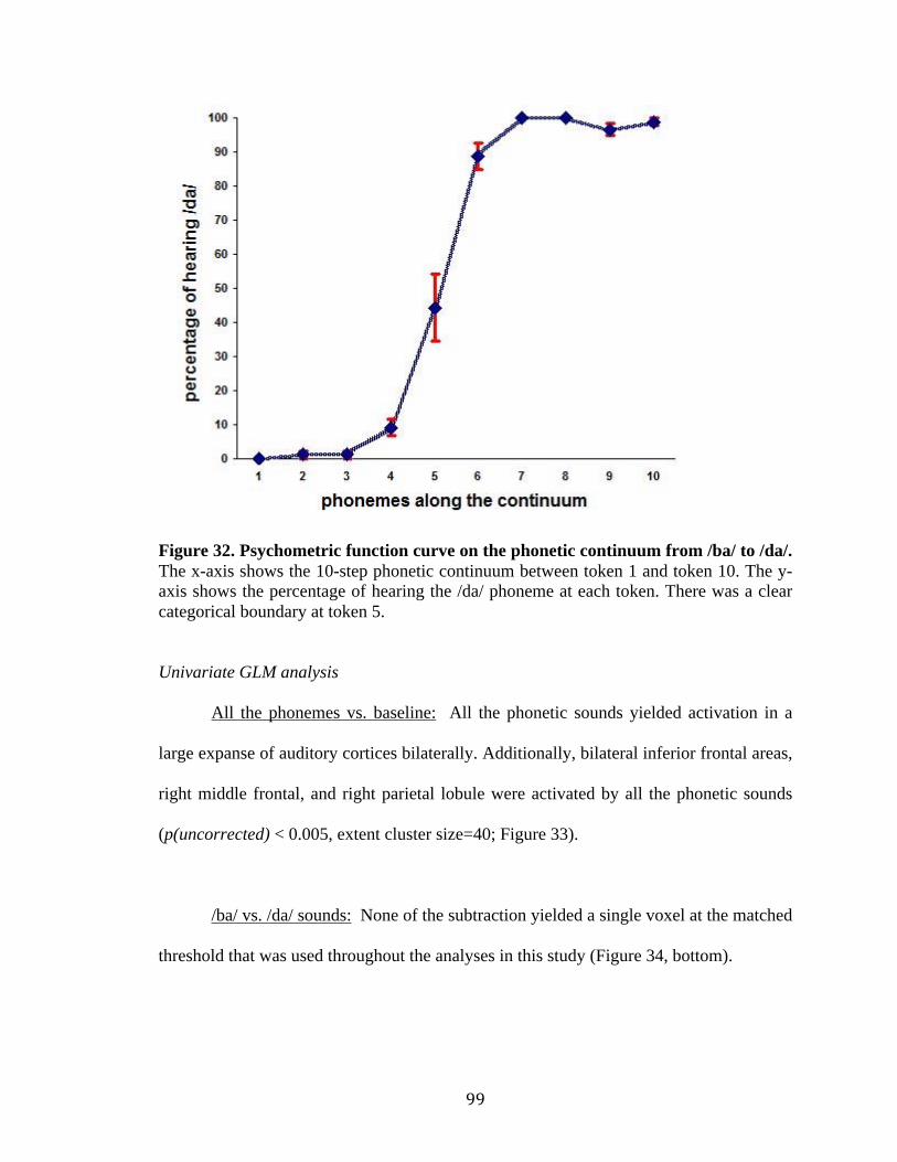
!!"
Figure 32. Psychometric function curve on the phonetic continuum from /ba/ to /da/.
The x-axis shows the 10-step phonetic continuum between token 1 and token 10. The y-
axis shows the percentage of hearing the /da/ phoneme at each token. There was a clear
categorical boundary at token 5.
Univariate GLM analysis
All the phonemes vs. baseline: All the phonetic sounds yielded activation in a
large expanse of auditory cortices bilaterally. Additionally, bilateral inferior frontal areas,
right middle frontal, and right parietal lobule were activated by all the phonetic sounds
(p(uncorrected) < 0.005, extent cluster size=40; Figure 33).
/ba/ vs. /da/ sounds: None of the subtraction yielded a single voxel at the matched
threshold that was used throughout the analyses in this study (Figure 34, bottom).

!""#
Figure 33. Group results of GLM showing areas more activated during the phoneme
listening conditions than at rest (p(uncorrected) < 0.005, extent cluster size=40) All
phonetic sounds yielded activation in the large expanse of bilateral auditory cortices.
Additional areas include bilateral inferior frontal gyrus, right middle frontal gyrus, and
right parietal lobe.
Multivariate analysis
All of /ba/ vs. /da/ sounds along the continuum: The searchlight analysis revealed
several brain regions that were scattered predominantly on the left hemisphere (Figure
34, top). The identified cortical regions were middle frontal gyrus, superior and inferior
parietal lobule, occipito-temporal junction, and posterior cingulate, as well as the lateral
occipital complex on the left hemisphere, anterior/posterior cingulate, and the calcarine
sulcus on the right hemisphere.

!"!#
Figure 34. Group results of MVPA (top) and GLM (bottom) showing areas that
distinguish between /ba/ and /da/ (p(uncorrected) <0.005, extent cluster size=40).
Whereas MVPA revealed several brain regions that produced categorical neural patterns
on the phonetic continuum, GLM did not yield any voxels at the matched threshold.
While this supports the second hypothesis (see the introduction), the weak result of GLM
may be due to the small number of subjects (n = 11).
Prototype /ba/ vs. /da/ sound comparison: The searchlight revealed that left
anterior and middle superior temporal gyri were the only areas for the prototype /ba/ and
/da/ comparison (Figure 35, bottom).

!"#$
Table 9. Brain regions identified by MVPA
No voxels were found by GLM at the chosen threshold (p(uncorrected) < 0.005, extent
cluster size=40)
Figure 35. Group results of MVPA (p(uncorrected) <0 .005, extent cluster size=40)
a (top row): Brain regions generating categorical neural patterns between all the phonetic
sounds that were perceived as /ba/ and all the phonemes that were perceived as /da/.
Several left-lateralized brain regions including middle frontal gyrus, superior and inferior
parietal lobule, occipito-temporal junction, inferior occipital gyrus, and anterior/posterior
cingulate were found. b (bottom row): Brain regions generating categorically distinct
neural patterns between two end points (token 1 & 2 vs. token 9 & 10). Anterior and
middle superior temporal gyri were found to distinguish between the phonemes at each
end. The results suggest their functional role in speech sound processing in the late (top)
and early (bottom) speech processing regions.

!"#$
Discussion
Neural basis of categorical phoneme perception
In this study, we examined the possible neural basis underlying categorical
phoneme perception with side-by-side use of GLM and MVPA. One plausible
mechanism would be that categorical perception may arise from the activation of
spatially segregated brain regions that are tuned to the acoustic characteristic of /ba/ and
/da/. It is well known that primary auditory cortex near Heschl’s gyrus has a tonotopic
arrangement for different ranges of sound frequencies (Talavage et al., 2004). We
hypothesized that a higher-level speech processing region downstream from A1 may be
organized in the same manner, which may be referred to as phonotopy. Although we
examined this hypothesis using the /ba/-/da/ continuum, the same rule could be applied to
categorical perception between /ba/ and /da/ and so on.
We tested this hypothesis with univariate GLM, but we did not find any spatially
distinct brain regions for /ba/ or /da/ representation. One parsimonious explanation of
such a result would be that the spatial scale of the /ba/ and /da/ mapping region is smaller
than the voxel scale that we employed (3x3x4mm). While future study may further
examine this possibility with a smaller scale of voxel size and a relatively reasonable
signal-to-noise ratio, we did not find any evidence of phonotopy.
Another explanation might be due to the small number of subjects resulting in
insufficient power for the 2nd
level random effect analysis using GLM. We initially
recruited 14 subjects, three of whom performed poorly during scanning (i.e., they failed
to press the button for the quieter sound more than half of the times [< 50%] whereas all

!"#$
the other subjects almost always detected the catch sound [98.1%]). As such, we had to
discard these three subjects' data from the analysis, resulting in only 11 subjects. It is
quite plausible that the GLM results would benefit from an increase in sample size and,
thus power.
The second plausible scenario would be that our categorical perception may come
from differential neural patterns that are generated by putative categorical phonetic
mapping regions. Two recent auditory fMRI studies support such a hypothesis.
Formisano et al. (2008) have shown that auditory cortices are able to distinguish a set of
vowel sounds (e.g., /a/, /i/, and /u/) in Dutch by eliciting differential neural patterns. More
recently, Raizada et al. (2009) were able to identify differential neural patterns between
/ra/ and /la/ in the right primary auditory cortex of the native English speaker while
neural responses of /ra/ and /la/ in this region were indistinguishable in the brains of
Japanese speakers in accordance with their inability of distinguishing /ba/ vs. /da/. Using
searchlight analysis (Kriegeskorte et al., 2006), we searched for brain regions that
generate a categorical response on the perceived phonetic continuum between /ba/ and
/da/. The searchlight revealed several cortical loci including middle frontal region,
superior and inferior parietal lobule, occipito-temporal junction, posterior cingulate, and
occipito lateral complex elicit categorical responses for the perceived /ba/ and /da/
phonetic sounds. While some areas were bilateral (e.g., cingulate and lateral occipital
complex), most brain regions were found in the left hemisphere, supporting the functional
specialization of left hemisphere for speech processing (Hickok & Poeppel, 2007).
Together, the results suggest that categorical perception may be achieved via overlapping
but differential neural responses within relevant brain areas. Future work is necessary to

!"#$
examine the joint contribution of each area that was identified by the current study.
Additionally, future fMRI studies may examine the functional connectivity of those areas
and EEG studies may examine the sequential organization of those areas for the
categorical phoneme processing.
The functional role of early vs. later speech processing area
The dichotomy between the results of using the whole phonetic continuum versus
each endpoint (the prototype /ba/ and /da/) is particularly interesting (Figure 35). The
current study demonstrated the functional role of early and late speech processing area by
comparing the entire phonetic continuums between the categorical boundary and two
tokens at each end that are always perceived as the prototype /ba/ and /da/. The former
case can be viewed as complex categorical processing to disambiguate subtle acoustic
differences along the continuum whereas the latter case can be viewed as rather
straightforward acoustic feature detection. Each comparison clearly yielded late and early
speech processing areas.
Among the regions found by comparing the entire phonetic continuum (Figure 34),
superior and inferior parietal lobules have been implicated in numerous reading and
speech studies, and this area is known to be involved in phonological mapping processing
(e.g., grapheme to phoneme; Booth et al., 1999, 2001, 2004, 2007; Bitan et al., 2007;
Dufor et al., 2007). For instance, Bitan et al. (2007) showed that conflict between
orthographic and phonological information resulted in a greater activation in the
superior/inferior parietal regions. Furthermore, a recent fMRI study comparing dyslexics
with normal subjects revealed that these parietal regions were not activated in dyslexia as

!"#$
much as in normal subjects during a phonetic discrimination task (Dufor et al., 2007).
Previous neuroimaging studies of phonological processing in adult dyslexics have
consistently reported a reduction or absence of activity in the left temporoparietal region
while performing an auditory phonological processing task (Rumsey et al., 1992; Temple
et al., 2003; Shaywitz & Shaywitz, 2003). Ruff et al. (2003) showed that right posterior
cingulate was not activated in adult dyslexic groups compared to normal groups when
two phonemes across the categorical boundary (i.e., /pa/-/ta/) were presented. Temple et
al. (2003) reported increased activation on the right anterior and posterior cingulate gyrus
after dyslexic children went through a remediation program involving phonological
awareness.
Additionally, it was observed that areas of visual cortex, such as inferior occipital
gyrus, generated categorical response to the phonetic sounds. While puzzling, the inferior
occipital area has been implicated as a visual word form area (VWFA) by numerous
reading studies (Allison et al., 1994; Nobre et al., 1994; Polk & Farah, 1998; Reinke et
al., 2008). In particular, the left inferior occipital region is preferentially activated by
words among many visual categories. It is possible that subjects may have implicitly
formed visual mental imagery of the corresponding phoneme while they heard /ba/ and
/da/ sounds during the scan.
The rationale of experimental design
It is important to emphasize that the paradigm in the present study differs from
many previous studies that typically involved an explicit speech phoneme task compared
with a control non-speech task (Hutchison et al., 2008; Oblesser et al., 2006; Uppenkamp
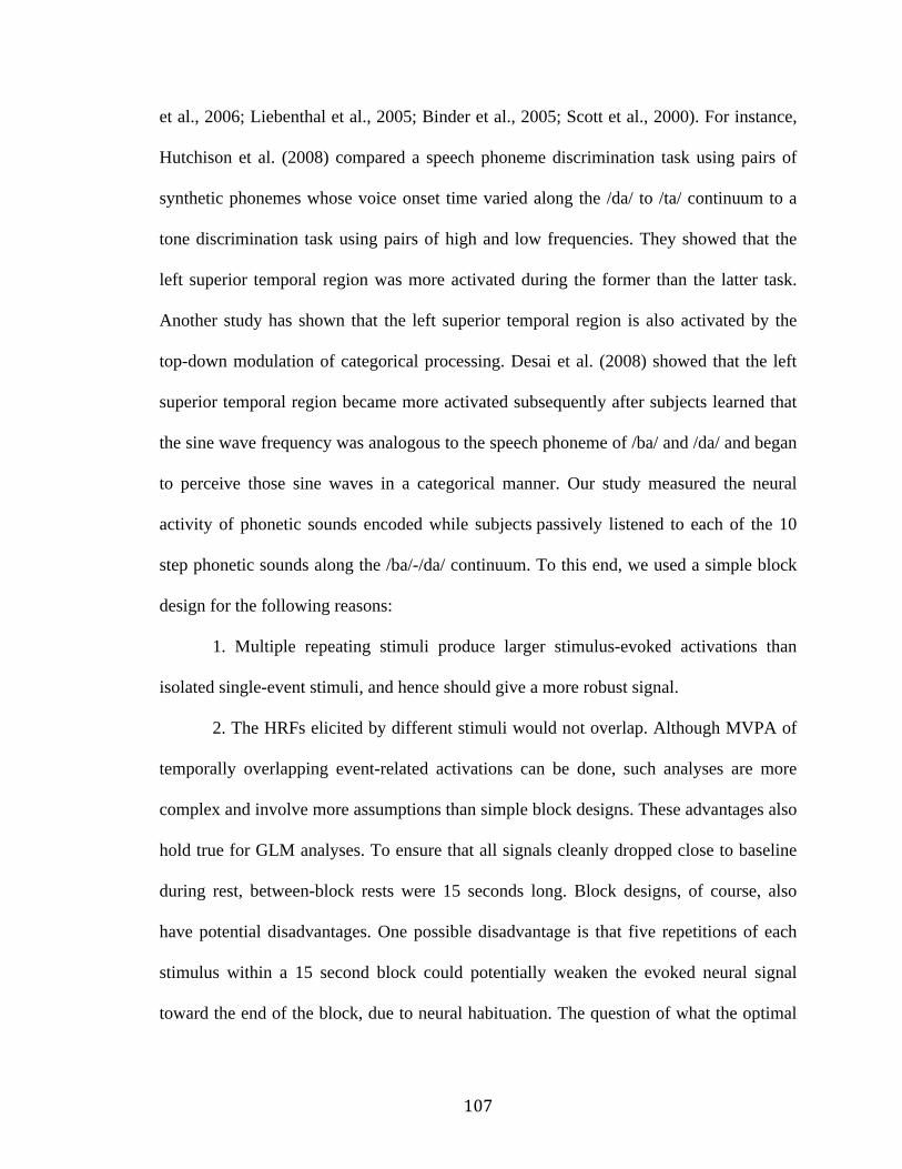
!"#$
et al., 2006; Liebenthal et al., 2005; Binder et al., 2005; Scott et al., 2000). For instance,
Hutchison et al. (2008) compared a speech phoneme discrimination task using pairs of
synthetic phonemes whose voice onset time varied along the /da/ to /ta/ continuum to a
tone discrimination task using pairs of high and low frequencies. They showed that the
left superior temporal region was more activated during the former than the latter task.
Another study has shown that the left superior temporal region is also activated by the
top-down modulation of categorical processing. Desai et al. (2008) showed that the left
superior temporal region became more activated subsequently after subjects learned that
the sine wave frequency was analogous to the speech phoneme of /ba/ and /da/ and began
to perceive those sine waves in a categorical manner. Our study measured the neural
activity of phonetic sounds encoded while subjects passively listened to each of the 10
step phonetic sounds along the /ba/-/da/ continuum. To this end, we used a simple block
design for the following reasons:
1. Multiple repeating stimuli produce larger stimulus-evoked activations than
isolated single-event stimuli, and hence should give a more robust signal.
2. The HRFs elicited by different stimuli would not overlap. Although MVPA of
temporally overlapping event-related activations can be done, such analyses are more
complex and involve more assumptions than simple block designs. These advantages also
hold true for GLM analyses. To ensure that all signals cleanly dropped close to baseline
during rest, between-block rests were 15 seconds long. Block designs, of course, also
have potential disadvantages. One possible disadvantage is that five repetitions of each
stimulus within a 15 second block could potentially weaken the evoked neural signal
toward the end of the block, due to neural habituation. The question of what the optimal

!"#$
block length for phonetic studies should be is an interesting area for future study, but is
beyond the scope of the present study. All in all, our results employing this experimental
design may be difficult to directly compare to previous studies involving explicit
categorization tasks and multiple phoneme presentations while measuring BOLD activity
most of which yielded activation in the left superior temporal region.
The limit of current studies
In this study, we attempted to perform a number of analyses with a given dataset
using both GLM and MVPA. As stated above, our lack of significant findings using
GLM could be due to the small sample size. An additional problem could be that these
data points may not be numerous enough for two additional MVPA: endpoints
comparison and near boundary phoneme comparison (Figure 35). The input data for these
two analyses were only 40% of the entire acquired dataset, which could also result in
different results. In particular, we were not able to find any voxels for the near-boundary
comparison at the matched threshold. Future studies could compare these with equal
amounts of data by properly re-designing the experiment. For example, using a between-
groups design (e.g., group 1 is assigned the full range of the phonetic continuum, group 2
is assigned the endpoints, and group 3 is assigned near the boundary), we could acquire
equal amounts of data that would provide enough power for MVPA.
Secondly, this study could not report the results using multiple correction
thresholds such as FDR (Genovese et al., 2002). While the identified regions have fairly
high separability t-values, it is necessary to validate their significance using some
alternative approaches such as non-parametric statistical mapping (Nichols & Holmes,

!"#$
2002) or the Monte Carlo random shuffling method (Metropolis & Ulman, 1949). For
more discussion of this issue, see the discussion in chapter 3 and also the general
discussion.
Lastly, the current study was not able to find a clear similarity structure among
the phonemes within the same category when we compared each pair of phonemes within
the identified areas. Future work is necessary to demonstrate the neural structure of each
phonetic sound within and across different categories.
$

!!"#
Chapter 5
General Discussion

!!!"
Implication of the findings in the thesis
The realm of auditory processing can be divided into three different sub-domains:
Processing of environmental sounds, human speech, and music. For the last several
decades, neuroscience has been focused on each auditory sub-domain separately; there
has been almost no attempt to consider these three aspects of auditory processing together
and to derive the integrated neural mechanisms underlying auditory processing. Within
each auditory sub-domain, the brain performs unique categorization processing.
Behavioral evidence of categorical perception has already been shown for each sub-
domain (Gygi et al., 2007; Johnsrude et al., 2000; Liberman et al., 1957). In one study
examining environmental sound categorization (Gygi et al., 2007), subjects were asked to
rate the similarity of two sounds in pair-wise combinations of 50 environmental sounds.
Multi-dimensional scaling (MDS) analysis was performed using the similarity ratings.
The results revealed a clear distinction between the animate and inanimate categories of
sounds. In the music domain, Johnsrude et al. (2000) showed that patients with lesions in
the right temporal lobe were not able to distinguish between ascending and descending
contours of melodic sequences, although they were able to discriminate whether the tones
were the same or different. The MDS analysis in our studies also revealed that melodies
within the same ascending or descending category tend to be judged similarly to melodies
across different categories (Figure 25). Lastly, in the speech domain, many studies have
demonstrated that speech phonemes are categorically perceived both by humans and non-
human primates (Liberman et al., 1957; Eimas et al., 1971; Kuhl & Padden, 1983).
!!"#
This thesis sought to find the neural basis for the behavioral manifestation of such
auditory categorization processing in each domain. As such, each chapter of the thesis
attempted to examine the following auditory categorization processes respectively:
- environmental sound categorization
$ musical sound categorization
$ speech phoneme categorization
The findings led us to a few concrete conclusions. First, regardless of type of sound,
the brain appears to utilize a unifying strategy for auditory categorization. That is,
different sound categories are represented through comparable but differential neural
patterns in their own distinct neural circuitries. For example, in the environmental sound
domain, our findings revealed that animate and inanimate sounds are categorized in the
large expanse of auditory cortices as well as several other non-temporal areas. In the
music domain, we revealed that ascending and descending melodies are categorically
represented by the right superior temporal sulcus, left inferior parietal lobule, and anterior
cingulate. Lastly, in the speech domain, our findings suggest that categorical perception
is achieved by differential neural patterns along a phonetic continuum within several left-
lateralized speech-processing areas.
The areas identified throughout the experiments correspond well to the findings
from previous GLM studies. For example, the anterior portion of the right superior
temporal sulcus was found to be involved in environmental sound processing by Zatorre
et al. (2004). In this study, they showed that this region was parametrically modulated by
the systematic variation of similarity across different environmental sounds. In the

!!"#
current study, we also found that the right aSTS elicited a robust separability pattern
between the animate and inanimate sound categories. (see Figure 36).
Figure 36. Left: adapted from Zatorre et al. (2004). In this PET imaging study, it was
found that the upper bank of right anterior STS was parametrically modulated by the
perceptual similarity ratings on the sounds that were systematically created by combining
45 different environmental sounds. Right: the group result (n=9) of whole brain
searchlight analysis showing the brain regions that distinguish between animate and
inanimate sound categories in the current study (P(FDR) < 0.05, extent cluster size=2).
The brighter yellow indicates stronger separability between animate and inanimate sound
categories, which is clearly seen in the anterior portion of the right STS. Both findings
confirm the notion suggested by anatomical and neurophysiological studies that the
anterior stream of the superior temporal lobe plays an important role for auditory object
processing.

!!"#
Our findings about the right superior temporal sulcus for melodic contour
processing also fit with several previous neuroimaging as well as lesion studies
(Johnsrude et al., 2000; Griffiths et al., 2004; Hyde et al., 2008; Perez & Zatorre, 2005).
For example, Zatorre et al. (1994) showed that the rSTS was more activated during a
melody listening condition than during a noise burst listening condition. Our findings
demonstrate that the rSTS is processing melodies by producing differential neural
responses (See figure 37).
The posterior parietal lobes and cingulate that we identified in chapter 4 have
been implicated in several previous dyslexia studies and visual reading studies. In
particular, the superior and inferior parietal areas are known to be involved in
phonological mapping processing (Booth et al., 1999, 2001, 2004, 2007; Bitan et al.,
2007; Dufor et al., 2007). Posterior cingulate is also known to play a crucial role in
phonological processing. For example, Temple et al. (2003) have shown that this area
was more activated after dyslexic children underwent an intensive intervention program.
Together, the findings throughout these chapters demonstrate that the brain regions that
are known to be involved in auditory processing in each sub-domain carry out categorical
processing through comparable but differential neural patterns.

!!"#
Figure 37. Left: adapted from Zatorre et al. (1994). In this PET imaging study, it was
found that CBF in rSTS was more increased during the melody listening condition than
during the noise burst listening condition. Right: the group result (n=12) of whole brain
searchlight analysis (P(uncorr.) <0.005, extent cluster size=10). Our results revealed that
rSTS (MNI: 51, -18, 17) was the best categorizer between ascending and descending
melodies among the areas that were found (see figure 26 in chapter 3). The current
MVPA study demonstrates that different melodies are distinguished via differential
neural patterns in the rSTS.
Secondly, throughout the experiments, our findings suggest a crossmodal link
between auditory and visual processing. The study on environmental sound
categorization revealed that several brain regions that have often been identified in vision
studies exhibit differential patterns for different auditory object categories. It is
conceivable that these areas may be triggered to readily identify if the sensory input is
from a “living organism” or “artifacts” independent of modality. Further, several visual
areas along the ventral visual cortex were found to distinguish between different auditory
object categories. The follow-up audio-visual categorization study found several

!!"#
downstream areas that distinguish between animate and inanimate categories for both
auditory and visual stimuli.
The study of musical melody categorization revealed that the inferior parietal
lobule, which is one of the key regions for the dorsal visual “where” pathway, is able to
categorize between ascending and descending melodies. A recent fMRI study by Foster
& Zatorre (2010) has shown that the inferior parietal sulcus was more activated during a
relative pitch judgment condition than during a passive melody listening task. They
argued that comparing the relative pitch distance of melodies that are on different keys
requires spatial processing in the left IPS. Together, the direction or relative size of pitch
distance may be processed by such a putative “universal spatial processing module” in
the brain. Follow-up study is necessary to better test the notion by using both auditory
and visual stimuli that share the same spatial properties.
The inferior occipital areas implicated in the speech categorization study (Chapter
4) also argue for cross-modal processing. The identified areas appear to be the “visual
word form area (VWFA)” that has been found by numerous visual reading studies
(Allison et al., 1994; Nobre et al., 1994; Polk & Farah, 1998; Reinke et al., 2008).
In sum, the thesis examined three specific cases – environmental sounds, musical
sounds, and speech sounds – of auditory categorization processing and discovered that
different categories are represented with differential neural patterns within each
categorization brain “module”. These auditory categorization areas are not confined to
the auditory cortex; other brain regions typically associated with visual processing also
participate in auditory processing. This suggests that object categorization may be

!!"#
achieved by crosstalk among areas at a supramodal level as sensory input is passed
toward the downstream regions, after it is extracted by its dedicated early sensory cortex.
GLM vs. MVPA (Testing different fundamental mechanisms of the brain)
As is described in the introduction, GLM and MVPA differ in their fundamental
approach. Depending on what hypothesis would be tested, either approach can be
effectively used. Throughout the experiments in the thesis, MVPA was mainly used to
test a particular hypothesis that different categories are represented through comparable
but differential neural patterns at the multi-voxel level. As a result, the searchlight
analysis revealed several distinct brain regions that produce differential neural patterns
across different categories. Nevertheless, all the data were also analyzed separately using
GLM analysis not only for the side-by-side comparison with MVPA results but also for
sanity checks to ensure data quality (e.g., empirically, subtracting [all the sound
conditions – baseline] should be able to yield activations in the bilateral superior and
middle temporal lobes.). In the case of more subtle analyses, e.g. animate – inanimate
(Chapter 2), ascending vs. descending (Chapter 3), and /ba/ vs. /da/ (Chapter 4), the GLM
results were, for the most part, weak and difficult to interpret except for the [animate-
inanimate] comparison which yielded activation in a large expanse of bilateral superior
and middle temporal lobe (see figure 13 in Chapter 2), In these cases, MVPA seemed to
offer a more complete picture of auditory object processing than traditional GLM
analyses.

!!"#
First, we conjecture that this can be largely attributed to the fundamental
mechanism of how the brain executes the categorization. Given the results of our study
and several previous studies (Lewis et al., 2005; Lewis et al., 2009), human auditory
cortices appear to be more sensitive to animate sound categories than inanimate sound
categories. It is quite conceivable that auditory cortices became attuned to animate
sounds throughout evolution, since those convey more critical information (e.g., prey and
predator, conspecific human voice, etc.). There is a human-voice-specific region within
the superior temporal lobes, just as we have a face-specific region within the ventral
temporal lobes (Belin & Zatorre, 2000; Kanwisher et al., 1997). Thus, it is obvious that
some neural substrates are reserved for the processing of stimuli that are crucial to our
survival. GLM has been proven to be a useful approach in successfully identifying those
areas.
Nonetheless, the brain does not seem to use only one strategy – preferential
activation by a specific category – for object categorization. Neuroimaging studies have
been exploring the possibilities by testing many other object categories using GLM. For
instance, Kanwisher stated that her group has been trying to identify brain regions for
more than 20 other different object categories (e.g., insect, tree, etc.) in addition to human
face, body, and house. They were not, however, able to find other category-specific brain
regions (at the Concept, Action, and Object workshop, Roverto, Italy 2010) (See
Downing et al., 1996 for more details). She also acknowledged the limits of using a
GLM that explicitly models brain activity using a canonical hemodynamic response. As a
consequence, GLM may have failed to identify areas that do not meet the assumed
model.

!!"#
The recently developed MVPA techniques suggested another neural mechanism
of object categorization by revealing that different categories are represented through
differential neural patterns within the same brain region (Haxby et al., 2001). These
regions can be also viewed as “categorization modules” which use different strategies to
encode objects from what face- or house-specific modules use. The advantage of
producing “differential” as opposed to “greater” neural response is that processing of
multiple different objects in one region may be detected. The brain may be evolved to
cope with myriad different objects in the world in such an efficient manner.
Together, both GLM and MVPA can be applied to reveal fundamentally different
neural mechanisms utilized by the brain. The present thesis was primarily focused on the
questions that MVPA may appropriately address. Throughout the experiments, we
demonstrated that MVPA can identify the brain regions that are invisible to GLM due to
their subtle BOLD activity differences across different categories.
However, the weak results of GLM analyses could also be attributed to the small
sample size in all the studies. The experiments in Chapter 2 had 9 and 11 subjects
respectively. The third study in Chapter 3 had 12 subjects, and the fourth study had 11
subjects. The rationale of choosing number of subjects around 9 - 12 was based upon the
previous MVPA literature and our experience from several pilot testing experiments.
Subject numbers around 10 provided enough power to yield a good result with MVPA
techniques. Nevertheless, this number of subjects may not be sufficient to provide enough
statistical power for GLM, which attempts to detect 1-5% of the BOLD signal difference
across different conditions. It is conceivable that GLM could have received some benefit
by increasing the subject numbers. Specifically, we acknowledge that GLM was limited

!"#$
in its ability to test the hypothesis that different phonetic categories may be represented
by different cortical loci in the speech categorization study, due to the small sample size.
Thus, future studies must employ a greater sample size (n> 15) if they aim to explore a
brain mechanism using both GLM and MVPA.
Distributed vs. localized brain mechanism (limit of the searchlight analysis)
While the chosen searchlight technique (Kriegeskorte et al., 2006) effectively
identified the brain areas that were involved in auditory categorization processing
throughout the studies, it must be acknowledged that it also has several limitations.
First, it cannot consider the joint contribution of non-adjacent regions, whereas
other methods can (e.g., recursive feature elimination); an excellent discussion of the
attendant dangers of potential overfitting can be found in Pereira et al. (2009). In
particular, RFE exhibits good generalization, by removing redundant (though
informative) voxels (Hanke et al., 2009), but the result will not show the full complement
of voxels that statistically distinguish between the stimuli of interest, which is what we
wished to show in the present thesis.
Second, as is the case for univariate GLM, the multiple correction must be
considered in the result of searchlight analysis since the analysis performs the
classification test at every single location of the brain on a voxel-by-voxel basis. While
FDR correction can be also applied in the searchlight result (Genovese et al., 2002), it is
still feasible to make the Type I error of losing significant voxels' areas under the
conservative threshold generated by multiple correction. In some of our studies, we were

!"!#
not able to report significant results using a multiple corrections threshold. For example,
in Chapter 3, the rSTS did not survive under FDR correction despite the fact that its
separability t-value after the 2nd
level random effect analysis was 7.71 (corresponding
uncorrected p-value is 0.000082 ). This is indeed more robust than several other areas
that survived under FDR correction in other studies in this thesis (see Table 3 in Chapter
2).
Lastly, the searchlight may inflate the result by repeatedly including the same set
of significant voxels. This is due to the fact that the searchlight is being moved on a
voxel-by-voxel basis to perform the classification test at every single location. Thus, if
one particular center voxel within the searchlight sphere yields high accuracy, it is likely
that the neighboring voxel will yield high accuracy as well since they share most of the
voxels surrounding them. An advanced searchlight method is necessary to avoid inflation
in the future.
The rationale of choosing threshold
In the thesis, different combinations of searchlight radius size, threshold p-value,
and size of extent cluster values were consistently applied throughout the studies to report
the results. Each threshold was chosen under the following steps. If any result did not
survive on the first criterion, it was considered in the next-most conservative criterion.

!""#
Step A
Exploring the data using size 0 through 3 searchlight radii (e.g., radius 1 refers to
one neighboring voxel from the center voxel) and determine the size of radius.
Radius 2 was chosen for the analysis of
audio-visual categorization (the second study in chapter 2)
ascending-descending (major-minor) melody categorization (chapter 3).
Radius 3 was chosen for the analysis of
auditory categorization at superordinate and each basic-level (the first
study in chapter 2)
ba/ vs. /da/ categorization (chapter 4).
Step B
Once the optimal searchlight radius was chosen, different p-values and
cluster sizes were considered.
i) Applying multiple correction (FDR 0.05) & large extent cluster size
: N/A
ii) Applying multiple correction & small extent cluster size
: - Animate vs. inanimate sound category classification (FDR 0.05, extent
cluster size=2)
- Within animate category classification (FDR 0.05, extent
cluster size=2)
ii) Applying multiple correction with no extent cluster size

!"#$
: - Animate vs. inanimate sound (image) categorization for audio-visual study
(P(FDR) <0.05)
iii) Applying uncorrected p-value with large extent cluster size
: - /ba/ vs. /da/ category classifcation test using whole continuum (P <0.005 &
extent cluster size =40)
- /ba/ vs. /da/ category classification using the end points. (P <0.005 & extent
cluster size =40)
iv) Applying uncorrected p-value with small extent cluster size
: - ascending vs. descending melody category classification (P <0.005 & extent
cluster size =10)
v) Applying less conservative uncorrected p-value with large extent cluster size.
: N/A
As was pointed out above with reference to the limits of the searchlight analysis,
surviving under the FDR correction does not necessarily imply that a particular brain
region is more robustly able to categorize than another brain region that does not survive
under the correction. In order to further validate the significance of a particular area,
other analyses such as non-parametric statistical mapping (SnPM) (Nichols and Holmes,
2002) or Monte Carlo shuffling (Metropolis & Ulman, 1949) should be considered. Both
SnPM and Monte Carlo ask if the observed accuracy can occur by chance after thousands
of multiple random shuffles. However, those approaches also have the downside that they
take an enormous amount of time even using today's most powerful computers. It is

!"#$
expected that the time necessary to analyze data using those alternative approaches will
be reduced as the technology advances.
$

!"#$
Chapter 6.
Conclusions

!"#$
Cognitive neuroscience has explored auditory categorization far less extensively
than it has explored visual categorization. This work attempts to remedy a relative
paucity of research on sound categorization. In particular, this thesis has sought to
understand how sound is categorically represented by the brain.
In Chapter 2, categorization of environmental sounds was examined. The first
study has found that there are level-specific categorization “modules” that can distinguish
different categories with differentiable neural patterns. The second study has shown that
several downstream brain areas can distinguish between animate and inanimate objects in
the auditory and visual domain.
In Chapter 3, categorization of musical sounds was examined. The study revealed
that ascending and descending melodies are categorized by rSTS, lSPL, and ACC via
differential neural patterns. These areas may distinguish the melodies based on the
melodies' structures, not their emotional content.
In Chapter 4, categorization of speech sounds was examined. The study found that
several left-lateralized downstream areas produced a categorical neural pattern on the
phonetic continuum. Further, the study has demonstrated the functional specialization of
early and late speech processing areas for simple acoustic feature detection and for
complex categorical processing respectively.
In sum, different categories of sound are represented via different neural patterns
in distinct neural circuitries in each auditory sub-domain. Strikingly, auditory
categorization "modules" were found in areas typically associated with visual processing,
not just within the temporal lobes. This suggests that object categorization and
recognition are mediated by crosstalk among areas in a supramodal manner. Thus,

!"#$
neuroscience would benefit from more interaction between experts in the visual and
auditory domains, because their areas of respective expertise do not, in fact, process
information independently.
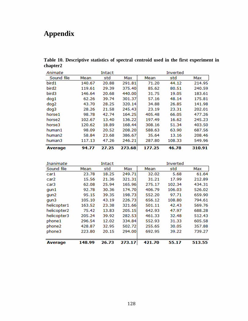
!"#$
Appendix
Table 10. Descriptive statistics of spectral centroid used in the first experiment in
chapter2

!"#$
Figure 38. Mean spectral centroid comparison between animate and inanimate
sounds in intact and inverted sound condition Mean spectral centroid is significantly
different between animate and inanimate sounds only in the inverted condition (t(22)=
2.9, p<0.05), not intact condition (t(22)=1.5, p>0.05). This is due to the fact that the
pivot frequency was chosen mostly in the higher frequency range that better makes the
inanimate sound unrecognizable.
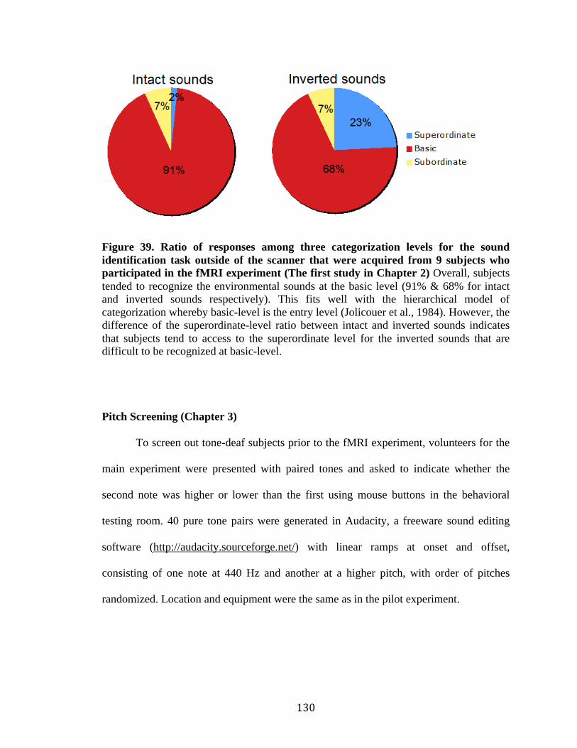
!"#$
Figure 39. Ratio of responses among three categorization levels for the sound
identification task outside of the scanner that were acquired from 9 subjects who
participated in the fMRI experiment (The first study in Chapter 2) Overall, subjects
tended to recognize the environmental sounds at the basic level (91% & 68% for intact
and inverted sounds respectively). This fits well with the hierarchical model of
categorization whereby basic-level is the entry level (Jolicouer et al., 1984). However, the
difference of the superordinate-level ratio between intact and inverted sounds indicates
that subjects tend to access to the superordinate level for the inverted sounds that are
difficult to be recognized at basic-level.
Pitch Screening (Chapter 3)
To screen out tone-deaf subjects prior to the fMRI experiment, volunteers for the
main experiment were presented with paired tones and asked to indicate whether the
second note was higher or lower than the first using mouse buttons in the behavioral
testing room. 40 pure tone pairs were generated in Audacity, a freeware sound editing
software (http://audacity.sourceforge.net/) with linear ramps at onset and offset,
consisting of one note at 440 Hz and another at a higher pitch, with order of pitches
randomized. Location and equipment were the same as in the pilot experiment.

!"!#
Procedures
Subjects were presented with paired tones and asked to indicate whether the
second note was higher or lower than the first using mouse buttons. Table 9 lists all the
tone pairs.
Results
All subjects fell into the normal range, thereby assuring that none of them were
tone-deaf.
Table 11. 20 stimulus pairs for the pitch-screening task (Chapter 3) Each pair was
played twice in the complete set.

!"#$
Figure 40. 4 odd-ball melodies that were required to be indicated by subjects during
the fMRI experiment in Chapter 4. The contour in the melodies is changed from
ascending to descending (a & b) or from descending to ascending direction (c & d).
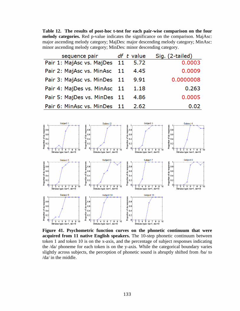
!""#
Table 12. The results of post-hoc t-test for each pair-wise comparison on the four
melody categories. Red p-value indicates the significance on the comparison. MajAsc:
major ascending melody category; MajDes: major descending melody category; MinAsc:
minor ascending melody category; MinDes: minor descending category.
Figure 41. Psychometric function curves on the phonetic continuum that were
acquired from 11 native English speakers. The 10-step phonetic continuum between
token 1 and token 10 is on the x-axis, and the percentage of subject responses indicating
the /da/ phoneme for each token is on the y-axis. While the categorical boundary varies
slightly across subjects, the perception of phonetic sound is abruptly shifted from /ba/ to
/da/ in the middle.
#
#
#
#

!"#$
References
$
Adams, R. B., & Janata, P. (2002). A comparison of neural circuits underlying auditory
and visual object categorization. NeuroImage, 16, 361-377.
Allison, T., McCarthy, G., Nobre, A., Puce, A., & Belger, A. (1994). Human extrastriate
visual cortex and the perception of faces, words, numbers, and colors. Cerebral
Cortex, 4(5), 544-554.
Ayotte, J., Peretz, I., & Hyde, K. (2002). Congenital amusia. A group study of adults
afflicted with a music-specific disorder. Brain, 125, 238-251.
Bartlett, J. C., & Dowling, W. J. (1980). Recognition of transposed melodies: a key-
distance effect in developmental perspective. Journal of Experimental Psychology
: Human Perception and Performance, 6, 501-515.
Belin, P., Zatorre, R. J., Hoge, R., Evans, A. C., & Pike, B. (1999). Event-related fMRI
of the auditory cortex. NeuroImage, 10, 417-429.
Belin, P., Zatorre, R. J., Lafille, P., Ahad, P., & Pike, B. (2000). Voice-selective areas
in human auditory cortex. Nature, 403, 309-312.

!"#$
Bengtsson, S. L., & Ullen, F. (2006). Dissociation between melodic and rhythmic
processing during piano performance from musical scores. Neuroimage, 30(1),
272-284.
Binder, J. R., Frost, J. A., Hammeke, T. A., Bellgowan, P. S., Springer, J. A., Kaufman, J.
N., & Possing, E. T. (2000). Human temporal lobe activation by speech and
nonspeech sounds. Cerebral Cortex, 10(5), 512-528.
Bitan, T., Burman, D. D., Chou, T. L., Lu, D., Cone, N. E., Cao, F., Bigio, J. D., &
Booth, J. R. (2007). The interaction between orthographic and phonological
information in children: an fmri study. Human Brain Mapping, 28(9), 880-891.
Blesser, B. (1972). Speech perception under conditions of spectral transformation. I.
Phonetic characteristics. Journal of Speech and Hearing Research, 15, 5-41.
Booth, J. R., Burman, D. D., Meyer, J. R., Gitelman, D. R., Parrish, T. B., & Mesulam,
M. M. (2004). Development of brain mechanisms for processing orthographic and
phonologic representations. Journal of Cognitive Neuroscience, 16(7), 1234-1249.
Booth, J. R., Burman, D. D., Van Santen, F. W., Harasaki, Y., Gitelman, D. R., Parrish,
T. B., & Marsel Mesulam, M. M. (2001). The development of specialized brain
systems in reading and oral-language. Child Neuropsychology, 7(3), 119-141.

!"#$
Booth, J. R., Cho, S., Burman, D. D., & Bitan, T. (2007). Neural correlates of mapping
from phonology to orthography in children performing an auditory spelling task.
Developmental Science, 10(4), 441-451.
Booth, J. R., Perfetti, C. A., & MacWhinney, B. (1999). Quick, automatic, and general
activation of orthographic and phonological representations in young readers.
Developmental Psychology, 35(1), 3-19.
Chao, L. L., Haxby, J. V., & Martin, A. (1999). Attribute-based neural substrates in
temporal cortex for perceiving and knowing about objects. Nature Neuroscience,
2(10), 913-919.
Cherry, E. C. (1953) Some experiments on the recognition of speech, with one and with
two ears. Journal of Acoustical Society of America, 25(5), 975-979
Cohen, Y. E. (2009). Multimodal activity in the parietal cortex. Hearing Research, 258,
100-105.
Cortes, C., & Vapnik, V.(1995). "Support-Vector Networks". Machine Learning, 20.
Crottaz-Herbette, S., & Menon, V. (2006). Where and when the anterior cingulate
modulates attentional response: Combined fMRI and ERP response. Journal of
cognitive neuroscience, 18, 766-780.

!"#$
Deng. L., & Huang, X. (2004). Challenges in adopting speech recognition.
Communication of the ACM, 47, 69-75.
Desai, R., Liebenthal, Waldron, E., & Binder, J. R. (2008). Left posterior temporal
regions are sensitive to auditory categorization. Journal of Cognitive
Neuroscience, 20, 1174-1188.
Di Pietro, M., Laganaro, M., Leemann, B., & Shnider, A. (2004). Receptive amusia:
temporal auditory processing deficit in a professional musician following a
left temporo-parietal lesion. Neuropsychologia, 42(7), 868-877.
Doehrmann, O., Naumer, M. J., Volz, S., Kaiser, J., and Altman, C. F. (2008). Probing
category selectivity for environmental sounds in the human auditory brain.
Neuropsychologia, 46, 2776-2786.
Dowling, W. J., & Fujitani, D. S. (1971). Contour, interval, and pitch recognition in
memory for melodies. Journal of Acoustic Society of America, 49, 524-531
Dowling, W. J., Lung, K. M., & Herrbold, S. (1987). Aiming attention in pitch and time
in the perception of interleaved melodies. Perception & psychophysics,
41, 642-656.

!"#$
Dowling, W. J. (1994). Melodic contour in hearing and remembering melodies. In
R. Aiello (Ed.), Musical perceptions, 173-190.
Dowling, W. J. (1978). Scale and contour: two components of a theory of memory for
music. Psychological Review, 85, 341-354.
Downing, P. E., Chan, A. W., Peelen, M. V., Dodds, C. M., & Kanwisher, N. (2006).
Domain specificity in visual cortex. Cereb Cortex, 16(10), 1453-1461.
Dufor, O., Serniclaes, W., Sprenger-Charolles, L., & Démonet, J. F. (2007). Top-down
processes during auditory phoneme categorization in dyslexia: a pet study.
NeuroImage, 34(4), 1692-1707.
Dufor, O., Serniclaes, W., Sprenger-Charolles, L., & Démonet, J. F. (2009). Left
premotor cortex and allophonic speech perception in dyslexia: a PET study.
NeuroImage, 46(1), 241-248.
Eimas, P. D., Siqueland, E. R., Jusczyk, P., & Vigorito, J. (1971). Speech perception in
infants. Science, 171(968), 303-306.
Engel, L. R., Frum, C., Puce, A., Walker, N. A., & Lewis, J. W. (2009). Different
categories of living and non-living sound-sources activate distinct cortical
networks. NeuroImage, 47, 1778-1791.

!"#$
Epstein, R., & Kanwisher, N. (1998). A cortical representation of the local visual
environment. Nature, 392, 598-601
Formisano, E., Martino, F. D., Bonte, M., & Goebel, R. (2008). “Who” is saying
“What”? Brain-based decoding of human voice and speech. Science, 322(5903),
970-973.
Foster, N. E. V., & Zatorre, R. J. (2010). A role for the intraparietal sulcus in
transforming musical pitch information. Cerebral Cortex, 20(6), 1350-1359.
Frey, S. H., Newman-Norlund, R. N., & Grafton, S. T. (2005). A distributed network in
the left cerebral hemisphere for planning everyday tool use skills. Cerebral
Cortex, 15, 681-695.
Gabrieli, J. D. (2009). Dyslexia: a new synergy between education and cognitive
neuroscience. Science, 325(5938), 280-283.
Gauthier, I., Skudlarski, P., Gore, J. C., & Anderson, A. W. (2000). Expertise for cars
and birds recruits brain areas involved in face recognition. Nature Neuroscience,
3, 191-197.

!"#$
Genovese, C. R., Lazar, N. A., & Nichols, T. (2002). Thresholding of statistical maps
in functional neuroimaging using the false discovery rate. NeuroImage, 15, 870-
878.
Griffiths, T., & Warren, D. (2004). What is an auditory object? Nature Reviews
Neuroscience, 5, 887-892.
Grill-Spector, K., Knouf, N., & Kanwisher, N. (2004). The fusiform face area subserves
face perception, not generic within-category identification. !"#$%&'!&$%()*+&,*&,
7 (5), 555-562.
Grill-Spector, K. (2003). The neural basis of object perception. Current Opinion in
Neurobiology, 13(2), 159-166.
Gygi, B., Kidd, G. R., & Watson, C. S. (2007). Similarity and categorization of
environmental sounds. Perception & Psychophysics, 69(6), 839-855.
Hackett, T. A., Stepniewsh, I., & Kaas, J. H. (1999). Prefrontal connections of the
parabelt auditory cortex in macaque monkeys. Brain Research, 817, 45-58.
Hanson, S. J., & Halchenko, Y. O. (2008). Brain reading using full brain support vector
machines for object recognition: There is no “face” identification area. Neural
Computation, 20, 486-503.

!"!#
Haxby, J. V., Gobbini, M. I., Furey, M. L., Ishai, A., Schouten, J. L., & Pietrini, P.
(2001). Distributed and overlapping representations of faces and objects in ventral
temporal cortex. Science. 293, 2425-2430.
Haynes, J. D., & Rees, G. (2005). Predicting the stream of consciousness from activity in
human visual cortex. Current Biology, 15, 1301-1307.
Hickok, G., & Poeppel, D. (2007). The cortical organization of speech processing. Nature
Neuroscience Review, 8, 393-402.
Hutchison, E. R., Blumstein, S. E., & Myers, E. B. (2008). An event-related fMRI
investigation of voice-onset time discrimination. NeuroImage, 40(1), 342-352.
Hyde, K. L., Peretz, I., & Zatorre, R. J. (2008). Evidence for the role of the right auditory
cortex in fine pitch resolution. Neuropsychologia, 46(2), 632-639.
Janata, P., & Grafton, S. (2003). Swinging in the brain: Shared neural substrates for
behaviors related to sequencing and music. Nature Neuroscience Review, 6, 682-
687.
Johnsrude, I., Penhune, V. B., & Zatorre, R. J. (2000). Functional specificity in the right
human auditory cortex for perceiving pitch direction. Brain, 123, 155-163.

!"#$
Jolicoeur, P., Gluck, M. A., & Kossyln, S. M. (1984). Pictures and names: making the
connection. Cognitive Psychology, 16(2), 243-275.
Kadosh, R. C., & Walsh, V. (2009). Numerical representation in the parietal lobes:
abstract or not-abstract? Behavoral & Brain Science, 32, 313-373.
Kamitani, Y., & Tong, F. (2005). Decoding the visual and subjective contests of the
human brain. Nature Neuroscience, 8, 679-685.
Kanwisher, N., McDermott, J., & Chun, M. M. (1997). "The fusiform face area: a module
in human extrastriate cortex specialized for face perception". Journal of
Neuroscience, 17, 4302-4311.
Kay, K. N., Naselaris, T., Prenger, R. J., & Gallant, J. L. (2008). Identifying natural
images from human brain activity. Nature, 452, 352-355.
Knosch, T., Neuhaus, C., & Haueisen, J. (2005). Perception of phrase structure in music.
Human Brain Mapping, 24, 259-273.
Kriegeskorte, N., & Bandettini, P. (2007). Analyzing for information, not activation, to
exploit high-resolution fMRI. NeuroImage, 38, 649-662.

!"#$
Kriegeskorte, N., Mur, M., Ruff, D., Kiani, R., Bodurka, J., Esteky, H., Tanaka, K., &
Bandettini, P. A. (2008). Matching categorical object representations in inferior
temporal cortex of man and monkey. Neuron, 60, 1126-1141.
Kuhl, P. K., & Padden, D. M. (1983). Enhanced discriminability at the phonetic
boundaries for the place feature in macaques. Journal of Acoustic Society of
America, 73, 1003-1007.
Lewis, J. W., Brefczynksi, J. A., Phinney, R. E., Janik, J., & DeYoe, E. (2005). Journal
of Neuroscience, 25(21), 5148-5158.
Lewis, J. W., Talkington, W. J., Walker, N. A., Spirou, G. A., Jajosky, A., Frum, C., &
Brefczynski-Lewis, J. A. (2009). Human cortical organization for processing
vocalizations indicates representation of harmonic structure as a signal attribute.
Journal of Neuroscience, 29(7), 2283-2296.
Liberman, A. M., Harris, K. S., Hoffman, H. S., & Griffith, B. C. (1957). The
discrimination of speech sounds within and across phoneme boundaries.
Journal of Experimental Psychology, 54(5), 358-368.
Liebenthal, E., Binder, J. R., Spitzer, S. M., Possing, E. T., & Medler, D. A. (2005).
Neural substrates of phonemic perception. Cerebral Cortex, 15, 1621-1631.

!""#
Liu, J., Harris, A., & Kanwisher, N. (2002). Stages of processing in face perception: an
MEG study. Nature Neuroscience, 5(9), 910-916.
Mangasarian, O. L., & Musicant, D. (2001). Lagrangian support vector machines.
Journal of Machine Learning Research, 1, 161–177.
Martin, A. (2007). The representation of object concepts in the brain. Annual Review
of Psychology, 58, 25-45.
Metropolis, N., & Ulam, S. (1949). The Monte Carlo method. Journal of American
Statistical Association, 44 (247), 335-341.
Milner, B. (1962). Laterality effects in audition. In Interhemispheric Relations and
Cerebrale Dominance, ed. VB Mountcastle, 177-195. Baltimore, MD:
Johns Hopkins Press.
Mishkin, M., Ungerleider, L. G., & Macko, K. A. (1983). Object vision and spatial
vision: Two cortical pathways. Trends in Neurosciences, 6, 414-417.
Mittershiffthaler, M., Fu, C., Dalton, J., Andrew C. M., & Williams, S. C. R. (2007). A
functional MRI study of happy and sad affective states induced by classical
music. Human Brain Mapping, 28, 1150-1162.

!"#$
Nichols, T. E., & Holmes, A. P. (2002). Nonparametric permutation tests for functional
neuroimaging: a primer with examples. Human Brain Mapping, 15, 1-25.
Nobre, A. C., Allison, T., & McCarthy, G. (1994). Word recognition in the human
inferior temporal lobe. Nature, 372(6503), 260-263.
Obleser, J., Boecker, H., Drzezga, A., Haslinger, B., Hennenlotter, A., Roettinger, M.,
Eulitz, C., & Rauschecker, J. P. (2006). Vowel sound extraction in anterior
superior temporal cortex. Human Brain Mapping, 27(7), 562-571.
Pereira, F., Mitchell, T., & Botvinick, M. (2009). Machine learning classifiers and fMRI:
A tutorial overview. Neuroimage, 45, 199-209.
Peretz, I., & Hyde, K. (2003). What is specific to music processing? Insights from
congenital amusia. Trends in Cognitive Science, 7(8), 362-367.
Plantinga, J., & Trainor, L. J. (2005). Memory for melody: infants use a relative pitch
code. Cognition, 98, 1-11.
Polk, T. A., & Farah, M. J. (1998). The neural development and organization of letter
recognition: evidence from functional neuroimaging, computational modeling,
and behavioral studies. Proceedings of Nattional Academy of Science U S A,
95(3), 847-852.

!"#$
Peretz, I., & Zatorre, R. J. (2005). Brain organization for music processing. Annual
Review of Psychology, 56, 89-114.
Raizada, R. D. S., Tsao, F. M., Liu, H. M., & Kuhl, P. K. (2009). Quantifying the
adequacy of neural representations for a cross-language phonetic discrimination
task: prediction of individual differences. Cerebral Cortex, 20(1), 1-12.
Rao, S. C., Rainer, G., & Miller, E. K., (1997). Integration of what and where in the
primate prefrontal cortex. Science, 276, 821-824.
Rauschecker, J. P. (1998). Parallel processing in the auditory cortex of primates.
Audiology & Neuro-otolgy, 3, 86-103.
Reinke, K., Fernandes, M., Schwindt, G., O'Craven, K., & Grady, C. L. (2008).
Functional specificity of the visual word form area: general activation for words
and symbols but specific network activation for words. Brain Language, 104(2),
180-189.
Romanski, L. M., Bates, J. F., & Goldman-Rakic, P. S. (1999). Auditory belt and
parabelt projections to the prefrontal cortex in the rhesus monkeys. Journal of
Comparative Neurology, 403, 141-157.

!"#$
Ruff, S., Marie, N., Celsis, P., Cardebat, D., & Démonet, J. F. (2003). Neural substrates
of impaired categorical perception of phonemes in adult dyslexics: an fMRI study.
Brain Cognition, 53(2), 331-334.
Rumsey, J. M., Andreason, P., Zametkin, A. J., Aquino, T., King, A. C., Hamburger,
S. D., Pikus, A., Rapoport, J. L., & Cohen, R. M. (1992). Failure to activate the
left temporoparietal cortex in dyslexia. An oxygen 15 positron emission
tomographic study. Archives of Neurology, 49(5), 527-534.
Schon, D., Anton, J. L., Roth, M., & Besson, M.(2002). An fMRI study of music sight-
reading. Neuroreport, 13, 2285-2289.
Schoroeder, C. E., & Foxe, J. J. (2002). The timing and laminar profile of converging
inputs to multisensory areas of the macaque neocortex. Cognitive Brain
Research, 14, 187-198.
Scott, L. S., Tanaka, J. W., Sheinberg, D. L., & Curran, T. (2006). A reevaluation of the
electrophysiological correlates of expert object processing. Journal of Cognitive
Neuroscience, 18(9), 1453-1465.
Scott, S. K., Blank, C. C., Rosen, S., & Wise, R. J. (2000). Identification of a pathway
for intelligible speech in the left temporal lobe. Brain, 123(12), 2400-2406.

!"#$
Staeren, N., Renvall, H., De Martino, F., Goebel, R., & Formisano, E. (2009). Sound
categories are represented as distributed patterns in the human auditory cortex.
Current Biology, 24, 498-502.
Shaywitz, S. E., & Shaywitz, B. A. (2003). Dyslexia (specific reading disability).
Biological Psychiatry, 24(5), 147-153.
Stewart, L., Overath, T., Warren, J. D., Foxton, J. M., & Griffiths, T. D. (2008). fMRI
evidence for a cortical hierarchy of pitch pattern processing. Public Library of
Science One, 1, 1-6.
Stokes, M., Thompson, R., Nobre, A. C., & Duncan, J. (2009). Shape-specific
preparatory activity mediates attention to targets in human visual cortex.
Proceedings of National Academy of Science, 106, 19569-19674.
Sugase, Y., Yamane, S., Ueno, S., & Kawano, K. (1999). Global and fine information
coded by single neurons in the temporal visual cortex. Nature, 400, 869-873.
Talavage, T. M., Sereno, M. I., Melcher, J. R., Ledden, P. J., Rosen, B. R., & Dale, A. M.
(2004). Tonotopic organization in human auditory cortex revealed by
progressions of frequency sensitivity. Journal of Neurophysiology, 91(3), 1282-
1296.

!"#$
Tanaka, J. W., & Taylor, M. (1991). Object categories and expertise: Is the basic level in
the eye of the beholder? Cognitive Psychology, 23, 457-482.
Temple, E. (2002). Brain mechanisms in normal and dyslexic readers. Current Opinion
Neurobiology, 12(2), 178-183.
.
Temple, E., Deutsch, G. K., Poldrack, R. A., Miller, S. L., Tallal, P., Merzenich, M.
M., & Gabrieli, J. D. E. (2003). Neural deficits in children with dyslexia
ameliorated by behavioral remediation: evidence from functional MRI.
Proceedings of National Academy of Science U S A, 100(5), 2860-2865.
Thirion, B., Duchesnay, E., Hubbard, E., Dubois, J., Poline, J. B., Lebihan, D., &
Dehaene, S. (2006). Inverse retinotopy: Inferring the visual content of
images from brain activation patterns. NeuroImage, 33(4), 1104-1116.
Trehub, S. E., Thorpe, L. A., & Morrongiello, B. A. (1987). Organizational processes
in infants’ perception of auditory patterns. Child Development, 58,741-749.
Uppenkamp, S., Johnsrude, I. S., Norris, D., Marslen-Wilson, W., & Patterson, R. D.
(2006). Locating the initial stages of speech-sound processing in human
temporal cortex. NeuroImage, 31(3), 1284-1296.

!"#$
Van Essen, D. (2005). A population-Average, Landmark- and Surface-based (PALS)
atlas of human cerebral cortex. NeuroImage, 28, 635-632.
Volkova, A., Trehub, S. E., & Schellengerg, E. G. (2006). Infants’ memory for musical
performances. Developmental Science, 9, 584-590.
Walther, D. B., Caddigan, E., Fei-Fei, L., & Beck, D. M. (2009). Natural Scene
Categories Revealed in Distributed Patterns of Activity in the Human Brain.
Journal of Neuroscience, 29, 10573-10581.
Warrier, C. M., & Zatorre, R. J. (2004). Right temporal cortex is critical for utilization of
melodies contextual cues in a pitch constancy task. Brain, 127, 1616-1625.
Wheatley, T., Milleville S. C., & Martin, A. (2007). Understanding animate agents:
Distinct role for the social network and mirror system. Psychological Science,
18, 469-474.
Zatorre, R. J., Bouffard, M., & Belin, P. (2004). Sensitivity to auditory object features in
human temporal neocortex. Journal of Neuroscience, 24(14), 3637-3642.
Zatorre, R. J. (1985). Discrimination and recognition of tonal melodies after unilateral
cerebral excisions. Neuropsychologia, 23, 31-41.

!"!#
Zatorre, R. J., Evans, A. C., & Meyer, E. (1994). Neural mechanism underlying melodic
perception and memory for pitch. Journal of Neuroscience, 14, 1908-1919.
Zatorre, R. J., & Gandour, J. T. (2008). Neural specializations for speech and pitch:
moving beyond the dichotomies. Philosophical !"#$%#&'()$%*)+*',-*.)/#0***
1)&(-'/*2, 363(1493), 1087-1104.
. #
#
#