neural and evolutionary computing - lecture 7 1 evolutionary programming the origins: l. fogel...

Neural and Evolutionary Computing - Lecture 7

1

Evolutionary ProgrammingThe origins:

L. Fogel (1960) – development of methods which generate automatically systems with some intelligent behavior; this methods are inspired by the natural evolution;

D. Fogel (1990) – in the last years the evolutionary programming became more oriented toward solving problems (optimization and design)

Particularities• Various encoding variants (e.g. real vectors, neural networks

structures)• Based only on mutation, no recombination• Current variants: self-adaptive


2

Evolutionary ProgrammingFirst (traditional) direction :- Evolve systems (e.g. finite state machine) with prediction

abilities- The fitness of such a structure is measured by analyzing the

behavior of the system = prediction abilities- Fitness-ul este o masura asociata comportamentului sistemului

Finite State Machines (FSM):

FSM = (S, I, O, T,s0)

S – set of states

I – input alphabet

O – output alphabet

T:SxI->SxO - transition rules

s0 – initial state


3

Evolutionary ProgrammingA simple test problem: design a FSM to check if a binary string has an even or an odd

numbers of elements equal to 1 (parity problem)

- S={even,odd}- I={0,1}- O={0,1}

FSM output: final state = 0 (the sequence has an even number of 1)

final state = 1 (the sequence has an odd number of 1)


4

Evolutionary ProgrammingState diagram = labeled directed graph

par impar

1/1

1/00/0

0/1

EP Design:- choose: S, I, O

Population initialization: generate random FSMs

- Generate labels for nodes- Generate arcs- Generate labels

Mutation:- Mutation of the output symbol- Redirect an arc (mutate the target

node)- Add/eliminate nodes- Change the initial state


5

Evolutionary ProgrammingMutation example: change the target node of an arc

par impar

1/1

1/00/0

0/1

par impar

1/1

1/0

0/0

0/1


6

Evolutionary Programming2. Prediction: design an FSM which receives a sequence of n

symbols (e.g. bits) and generates the following symbol in the sequence.

1/0A

B

C

1/1

0/10/1

1/1

0/0 Input sequence:

0 1 1 1 0 1

CBC A AB States

1 1 0 1 1 1 Ouputs


7

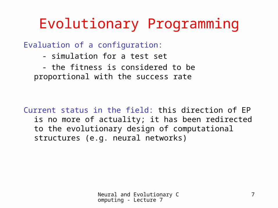
Evolutionary ProgrammingEvaluation of a configuration:

- simulation for a test set

- the fitness is considered to be proportional with the success rate

Current status in the field: this direction of EP is no more of actuality; it has been redirected to the evolutionary design of computational structures (e.g. neural networks)


8

Evolutionary ProgrammingSecond (current) direction: it is related to optimization methods

similar to evolution strategies

- there is only a mutation operator (no recombination)- the mutation is based on random perturbation of the current configuration (x’=x+N(0,s))

- s is inversely correlated with the fitness value (high fitness leads to small s, low fitness leads to large values for s)

- starting from a population with m elements, by mutation are constructed m children and the survivors are selected from the 2m elementst by tournament or simply truncation.

- There are self-adaptive variants, called MetaEP; these variants are similar to self-adaptive Evolution Strategies


9

Evolutionary ProgrammingMetaEP

)1.0(''

2.0 )),1.0(1('

)',...,',',...,'(),...,,,...,( 1111

Nsxx

Nss

ssxxssxx

iii

ii

nnnn

Remark: currently the normal mutation used to self-adapt the control parameters has been replaced with a log-normal distribution (as in the case of SE)


10

Genetic ProgrammingPrincipal contributor: J. Koza (1990)

Official web site: www.genetic-programming.org

• GP is an automated method for creating a working computer program from a high-level problem statement of a problem.

• GP starts from a high-level statement of “what needs to be done” and automatically creates a computer program to solve the problem.

http://www.genetic-programming.org/


11

Genetic Programming


12

Genetic ProgrammingNumeric regression

Input data: - pairs of values: (arg, val) - model which depends on

some parameters(e.g.: linear model, quadratic model etc)

Output: values of the model parameters valori ale parametrilor specifici modelului

Symbolic regression

Input data:

- pairs of values : (arg, val)

- terminals alphabet (variables, constants) and nonterminals (operators, functions)

Output: expression which describes the dependence between output variable (predicted value) and the input variable (predictor)


13

Genetic ProgrammingNumerical regression

Input data:

(1,3),(2,5),(3,7),(4,9)

Model: f(x)=ax+b

Result: a=2 b=1

Search in the parameter

space

Symbolic regression

Input data:

(1,3),(2,5),(3,7),(4,9)

Alphabet: +,*,-,/,constants,x

Result: 2*x+1

Search in the space of expressions

http://alphard.ethz.ch/gerber/approx/default.html


14

Genetic ProgrammingEncoding: the individuals are usually tree-like structures

Example 1: arithmetical expression

a*b+sin(c)

Components:

Nonterminals: operators and functions

Terminals: variables, constants (fixed or randomly generated), 0-arity functions

+

*

a b c

sin

Prefixed form: +*a b sin c (preorder )

Postfixed form: a b * c sin + (postorder)


15

Genetic ProgrammingEncoding: the individuals are usually tree-like structures

Example 2: C code

s=0;

i=0;

while (i<n)

{ i=i+1;

s=s+i;

}

;

;

= =

s 0 i 0

while

<

i n

;

=

i i+1

s=s+i

Problem: the tree representation can be complex even for simple programs


16

Genetic Programming

Summary: the terminals and nonterminals sets are chosen depending on the problem to be solved


17

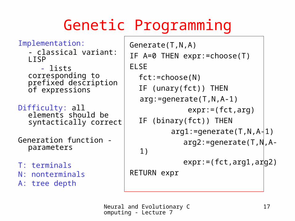
Genetic ProgrammingImplementation:

- classical variant: LISP - lists corresponding to

prefixed description of expressions

Difficulty: all elements should be syntactically correct

Generation function - parameters

T: terminalsN: nonterminalsA: tree depth

Generate(T,N,A)

IF A=0 THEN expr:=choose(T)

ELSE

fct:=choose(N)

IF (unary(fct)) THEN

arg:=generate(T,N,A-1)

expr:=(fct,arg)

IF (binary(fct)) THEN

arg1:=generate(T,N,A-1)

arg2:=generate(T,N,A-1)

expr:=(fct,arg1,arg2)

RETURN expr


18

Genetic ProgrammingOther variants:

• Decision trees

• If-then rules

• Neural networks

• Logical expressions

• Binary decision diagrams

• Grammars


19

Genetic ProgrammingOther encoding variants:

• Linear Genetic Programming

• Gene Expression Programming

• Multi-expression Programming

• Grammar Evolution


20

Genetic ProgrammingLinear Genetic Programming [Brameier, Banzhaf, 2003]

Particularities:

- Used to generate programs as sequences of lines (e.g. like in assembling languages)

- The operations involves registers

- Instructions: if and goto

- The commented lines correspond to processing steps which do not influence the final result (similar to noncoding portions of DNA – the so-called introns)

- Crossover: uses a variant of single point crossover adapted for chromosomes with different lengths (the program is a chromosome, each line is a gene)


21

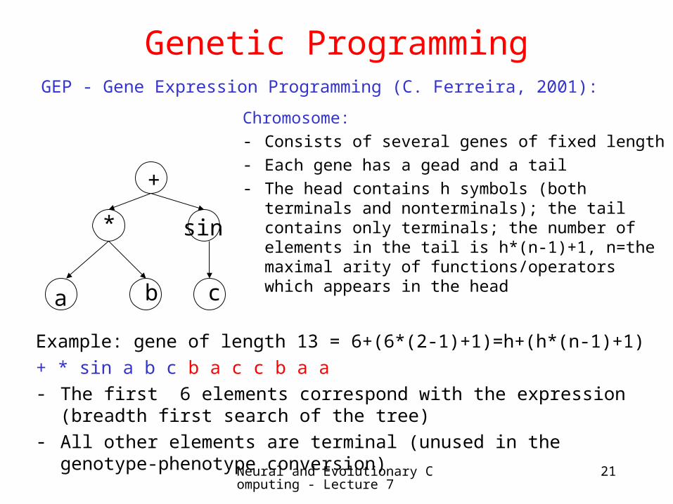
Genetic ProgrammingGEP - Gene Expression Programming (C. Ferreira, 2001):

+

*

a b c

sin

Chromosome:- Consists of several genes of fixed length - Each gene has a gead and a tail - The head contains h symbols (both terminals

and nonterminals); the tail contains only terminals; the number of elements in the tail is h*(n-1)+1, n=the maximal arity of functions/operators which appears in the head

Example: gene of length 13 = 6+(6*(2-1)+1)=h+(h*(n-1)+1)

+ * sin a b c b a c c b a a - The first 6 elements correspond with the expression (breadth first

search of the tree) - All other elements are terminal (unused in the genotype-phenotype

conversion)


22

Genetic ProgrammingGEP: allow to generate syntactically correct expressions by

extending the head over the symbols in the tail

+

*

a b c

sin

+

*

a b c

+

b

+ * sin a b c b a c c b a a + * + a b c b a c c b a a


23

Genetic ProgrammingGEP: chromosome consisting of two genes:+ * sin a b c b a c c b a a * * / a b c b a c c b a a

The phenotype corresponding to the chromosome is obtained by combining the genes corresponding to the two genes

+

*

a b c

sin

*

*

a b c

/

b

*


24

Genetic Programming

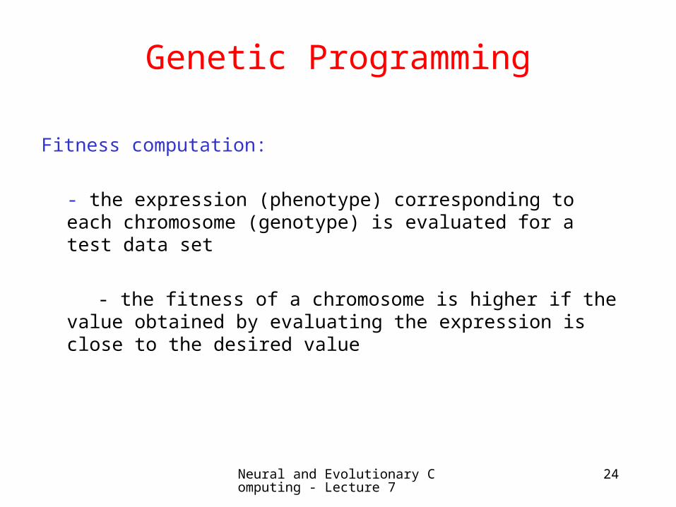
Fitness computation:

- the expression (phenotype) corresponding to each chromosome (genotype) is evaluated for a test data set

- the fitness of a chromosome is higher if the value obtained by evaluating the expression is close to the desired value


25

Genetic ProgrammingEvaluation:


26

Genetic ProgrammingCrossover: two parents (trees) generate two offspring (also trees) by swapping some subtrees

+

*

a b c

sin

*

-

a b 2

*

exp

c

a*b+sin(c) (a-b)*2*exp(c)


27

Genetic ProgrammingCrossover: two parents (trees) generate two offspring (also trees) by

swapping some subtrees

+

exp

c

sin

*

-

a b 2

*

*

a

exp(c)+sin(c) (a-b)*(2*(a*b))

c

b


28

Genetic Programming

Crossover:

Prefixed forms of parents and children

+ * a b sin c * - a b * 2 exp c

+ exp c sin c * - a b * 2 * a b

Remark. It is similar to the crossover used at GAs but the size for exchanged portions are usually different.


29

Genetic ProgrammingMutation: consists of randomly changing some elements

• Change the symbol of a leaf node with another terminal symbol (in the case of constants this mutation could be as in the case of evolution strategies)

• Replace a leaf node with a tree (growing mutation)

• Replace the symbol corresponding to an internal node with another nonterminal from the same class (function with the same arity)

• Replace a subtree with a terminal node (pruning mutation)

Remark: the mutation can be implemented by a crossover with a randomly generated element


30

Genetic Programming

Mutation: consists of randomly changing some elements

+

*

a b c

sin

+

*

2 b c

sin

+

*

a b -

sin

c 1


31

Genetic Programming

Bloat problem: the complex structures become dominant in the population

Solutions: • Use a threshold for the structure complexity (e.g. tree depth) and

reject all structures larger (deeper) than the threshold

• Use a penalty term depending on the structure complexity in the fitness computation; this term will penalize the complex structures


32

Genetic Programming

Applications:

• Extracting models from data (e.g. predictive models)

• Extracting rules from data

• Electrical circuits design

• Robust systems synthesis

• Evolvable hardware


33

Genetic Programming

• parallel applications design

• cellular automata design

• signal/image processing filters design

• generation of multi-agent strategies

• generation of game strategies

• generation of quantum algorithms

neural and evolutionary computing - lecture 7 1 evolutionary programming the origins: l. fogel...

Documents

neural networks structures

final state

small s

labels mutation

ouputs slide

fsm output

mutation operator

prediction abilities