networks computer analysis of performance

Matthew N.O. Sadiku · Sarhan M. Musa

Performance Analysis of Computer Networks

Performance Analysis of Computer Networks

Matthew N.O. Sadiku • Sarhan M. Musa

Performance Analysisof Computer Networks

Matthew N.O. SadikuRoy. G. Perry College of EngineeringPrairie View A&M UniversityPrairie View, TX, USA

Sarhan M. MusaRoy. G. Perry College of EngineeringPrairie View A&M UniversityPrairie View, TX, USA

ISBN 978-3-319-01645-0 ISBN 978-3-319-01646-7 (eBook)DOI 10.1007/978-3-319-01646-7Springer Cham Heidelberg New York Dordrecht London

Library of Congress Control Number: 2013947166

© Springer International Publishing Switzerland 2013This work is subject to copyright. All rights are reserved by the Publisher, whether the whole or partof the material is concerned, specifically the rights of translation, reprinting, reuse of illustrations,recitation, broadcasting, reproduction on microfilms or in any other physical way, and transmission orinformation storage and retrieval, electronic adaptation, computer software, or by similar or dissimilarmethodology now known or hereafter developed. Exempted from this legal reservation are brief excerptsin connection with reviews or scholarly analysis or material supplied specifically for the purpose of beingentered and executed on a computer system, for exclusive use by the purchaser of the work. Duplicationof this publication or parts thereof is permitted only under the provisions of the Copyright Law of thePublisher’s location, in its current version, and permission for use must always be obtained fromSpringer. Permissions for use may be obtained through RightsLink at the Copyright Clearance Center.Violations are liable to prosecution under the respective Copyright Law.The use of general descriptive names, registered names, trademarks, service marks, etc. in thispublication does not imply, even in the absence of a specific statement, that such names are exemptfrom the relevant protective laws and regulations and therefore free for general use.While the advice and information in this book are believed to be true and accurate at the date ofpublication, neither the authors nor the editors nor the publisher can accept any legal responsibility forany errors or omissions that may be made. The publisher makes no warranty, express or implied, withrespect to the material contained herein.

Printed on acid-free paper

Springer is part of Springer Science+Business Media (www.springer.com)

To my late dad, Solomon, late mom, Ayisat,and my wife, Kikelomo.

To my late father, Mahmoud,mother, Fatmeh, and my wife, Lama.

Preface

Modeling and performance analysis play an important role in the design of

computer communication systems. Models are tools for designers to study a system

before it is actually implemented. Performance evaluation of models of computer

networks during the architecture design, development, and implementation stages

provides means to assess critical issues and components. It gives the designer the

freedom and flexibility to adjust various parameters of the network in the planning

rather than in the operational phase.

The major goal of the book is to present a concise introduction to the perfor-

mance evaluation of computer communication networks. The book begins by

providing the necessary background in probability theory, random variables, and

stochastic processes. It introduces queueing theory and simulation as the major

tools analysts have at their disposal. It presents performance analysis on local,

metropolitan, and wide area networks as well as on wireless networks. It concludes

with a brief introduction to self-similarity.

The book is designed for a one-semester course for senior-year undergraduate and

graduate engineering students. The prerequisite for taking the course is a background

knowledge of probability theory and data communication in general. The book can be

used in giving short seminars on performance evaluation. It may also serve as a fingertip

reference for engineers developing communication networks, managers involved in

systems planning, and researchers and instructors of computer communication networks.

We owe a debt of appreciation to Prairie View A&M University for providing

the environment to develop our ideas. We would like to acknowledge the support of

the departmental head, Dr. John O. Attia, and college dean, Dr. Kendall Harris.

Special thanks are due to Dr. Sadiku’s graduate student, Nana Ampah, for carefully

going through the entire manuscript. (Nana has graduated now with his doctoral

degree.) Dr. Sadiku would like to thank his daughter, Ann, for helping in many

ways especially with the figures. Without the constant support and prayers of our

families, this project would not have been possible.

Prairie View, TX, USA Matthew N.O. Sadiku

Prairie View, TX, USA Sarhan M. Musa

vii

Contents

1 Performance Measures . . . . . . . . . . . . . . . . . . . . . . . . . . . . . . . . . . 1

1.1 Computer Communication Networks . . . . . . . . . . . . . . . . . . . . . 1

1.2 Techniques for Performance Analysis . . . . . . . . . . . . . . . . . . . . 2

1.3 Performance Measures . . . . . . . . . . . . . . . . . . . . . . . . . . . . . . . 3

References . . . . . . . . . . . . . . . . . . . . . . . . . . . . . . . . . . . . . . . . . . . . 4

2 Probability and Random Variables . . . . . . . . . . . . . . . . . . . . . . . . . 5

2.1 Probability Fundamentals . . . . . . . . . . . . . . . . . . . . . . . . . . . . . 5

2.1.1 Simple Probability . . . . . . . . . . . . . . . . . . . . . . . . . . . . . 6

2.1.2 Joint Probability . . . . . . . . . . . . . . . . . . . . . . . . . . . . . . 8

2.1.3 Conditional Probability . . . . . . . . . . . . . . . . . . . . . . . . . 8

2.1.4 Statistical Independence . . . . . . . . . . . . . . . . . . . . . . . . . 9

2.2 Random Variables . . . . . . . . . . . . . . . . . . . . . . . . . . . . . . . . . . 11

2.2.1 Cumulative Distribution Function . . . . . . . . . . . . . . . . . . 12

2.2.2 Probability Density Function . . . . . . . . . . . . . . . . . . . . . 13

2.2.3 Joint Distribution . . . . . . . . . . . . . . . . . . . . . . . . . . . . . . 14

2.3 Operations on Random Variables . . . . . . . . . . . . . . . . . . . . . . . 20

2.3.1 Expectations and Moments . . . . . . . . . . . . . . . . . . . . . . . 20

2.3.2 Variance . . . . . . . . . . . . . . . . . . . . . . . . . . . . . . . . . . . . 22

2.3.3 Multivariate Expectations . . . . . . . . . . . . . . . . . . . . . . . . 22

2.3.4 Covariance and Correlation . . . . . . . . . . . . . . . . . . . . . . 23

2.4 Discrete Probability Models . . . . . . . . . . . . . . . . . . . . . . . . . . . 28

2.4.1 Bernoulli Distribution . . . . . . . . . . . . . . . . . . . . . . . . . . 28

2.4.2 Binomial Distribution . . . . . . . . . . . . . . . . . . . . . . . . . . 29

2.4.3 Geometric Distribution . . . . . . . . . . . . . . . . . . . . . . . . . 30

2.4.4 Poisson Distribution . . . . . . . . . . . . . . . . . . . . . . . . . . . . 31

2.5 Continuous Probability Models . . . . . . . . . . . . . . . . . . . . . . . . . 33

2.5.1 Uniform Distribution . . . . . . . . . . . . . . . . . . . . . . . . . . . 33

2.5.2 Exponential Distribution . . . . . . . . . . . . . . . . . . . . . . . . 34

2.5.3 Erlang Distribution . . . . . . . . . . . . . . . . . . . . . . . . . . . . 34

ix

2.5.4 Hyperexponential Distribution . . . . . . . . . . . . . . . . . . . 35

2.5.5 Gaussian Distribution . . . . . . . . . . . . . . . . . . . . . . . . . . 35

2.6 Transformation of a Random Variable . . . . . . . . . . . . . . . . . . . 40

2.7 Generating Functions . . . . . . . . . . . . . . . . . . . . . . . . . . . . . . . 42

2.8 Central Limit Theorem . . . . . . . . . . . . . . . . . . . . . . . . . . . . . . 44

2.9 Computation Using MATLAB . . . . . . . . . . . . . . . . . . . . . . . . 46

2.9.1 Performing a Random Experiment . . . . . . . . . . . . . . . . 46

2.9.2 Plotting PDF . . . . . . . . . . . . . . . . . . . . . . . . . . . . . . . . 47

2.9.3 Gaussian Function . . . . . . . . . . . . . . . . . . . . . . . . . . . . 48

2.10 Summary . . . . . . . . . . . . . . . . . . . . . . . . . . . . . . . . . . . . . . . . 51

Problems . . . . . . . . . . . . . . . . . . . . . . . . . . . . . . . . . . . . . . . . . . . . . 52

References . . . . . . . . . . . . . . . . . . . . . . . . . . . . . . . . . . . . . . . . . . . . 58

3 Stochastic Processes . . . . . . . . . . . . . . . . . . . . . . . . . . . . . . . . . . . . 61

3.1 Classification of Random Processes . . . . . . . . . . . . . . . . . . . . . 62

3.1.1 Continuous Versus Discrete Random Process . . . . . . . . 63

3.1.2 Deterministic Versus Nondeterministic

Random Process . . . . . . . . . . . . . . . . . . . . . . . . . . . . . 63

3.1.3 Stationary Versus Nonstationary Random Process . . . . . 63

3.1.4 Ergodic Versus Nonergodic Random Process . . . . . . . . 64

3.2 Statistics of Random Processes and Stationarity . . . . . . . . . . . . 65

3.3 Time Averages of Random Processes and Ergodicity . . . . . . . . 71

3.4 Multiple Random Processes . . . . . . . . . . . . . . . . . . . . . . . . . . 72

3.5 Sample Random Processes . . . . . . . . . . . . . . . . . . . . . . . . . . . 75

3.5.1 Random Walks . . . . . . . . . . . . . . . . . . . . . . . . . . . . . . 75

3.5.2 Markov Processes . . . . . . . . . . . . . . . . . . . . . . . . . . . . 76

3.5.3 Birth-and-Death Processes . . . . . . . . . . . . . . . . . . . . . . 77

3.5.4 Poisson Processes . . . . . . . . . . . . . . . . . . . . . . . . . . . . 78

3.6 Renewal Processes . . . . . . . . . . . . . . . . . . . . . . . . . . . . . . . . . 80

3.7 Computation Using MATLAB . . . . . . . . . . . . . . . . . . . . . . . . 80

3.8 Summary . . . . . . . . . . . . . . . . . . . . . . . . . . . . . . . . . . . . . . . . 83

Problems . . . . . . . . . . . . . . . . . . . . . . . . . . . . . . . . . . . . . . . . . . . . . 83

References . . . . . . . . . . . . . . . . . . . . . . . . . . . . . . . . . . . . . . . . . . . . 86

4 Queueing Theory . . . . . . . . . . . . . . . . . . . . . . . . . . . . . . . . . . . . . . 87

4.1 Kendall’s Notation . . . . . . . . . . . . . . . . . . . . . . . . . . . . . . . . . 88

4.2 Little’s Theorem . . . . . . . . . . . . . . . . . . . . . . . . . . . . . . . . . . . 89

4.3 M/M/1 Queue . . . . . . . . . . . . . . . . . . . . . . . . . . . . . . . . . . . . . 91

4.4 M/M/1 Queue with Bulk Arrivals/Service . . . . . . . . . . . . . . . . 96

4.4.1 Mx/M/1 (Bulk Arrivals) System . . . . . . . . . . . . . . . . . . 97

4.4.2 M/MY/1 (Bulk Service) System . . . . . . . . . . . . . . . . . . 98

4.5 M/M/1/k Queueing System . . . . . . . . . . . . . . . . . . . . . . . . . . . 99

4.6 M/M/k Queueing System . . . . . . . . . . . . . . . . . . . . . . . . . . . . 100

4.7 M/M/1 Queueing System . . . . . . . . . . . . . . . . . . . . . . . . . . . . 102

x Contents

4.8 M/G/1 Queueing System . . . . . . . . . . . . . . . . . . . . . . . . . . . . . 103

4.9 M/Ek/1 Queueing System . . . . . . . . . . . . . . . . . . . . . . . . . . . . 106

4.10 Networks of Queues . . . . . . . . . . . . . . . . . . . . . . . . . . . . . . . . 107

4.10.1 Tandem Queues . . . . . . . . . . . . . . . . . . . . . . . . . . . . . 107

4.10.2 Queueing System with Feedback . . . . . . . . . . . . . . . . 109

4.11 Jackson Networks . . . . . . . . . . . . . . . . . . . . . . . . . . . . . . . . . . 109

4.12 Summary . . . . . . . . . . . . . . . . . . . . . . . . . . . . . . . . . . . . . . . . 110

Problems . . . . . . . . . . . . . . . . . . . . . . . . . . . . . . . . . . . . . . . . . . . . . 111

References . . . . . . . . . . . . . . . . . . . . . . . . . . . . . . . . . . . . . . . . . . . . 113

5 Simulation . . . . . . . . . . . . . . . . . . . . . . . . . . . . . . . . . . . . . . . . . . . . 115

5.1 Why Simulation? . . . . . . . . . . . . . . . . . . . . . . . . . . . . . . . . . . 116

5.2 Characteristics of Simulation Models . . . . . . . . . . . . . . . . . . . . 117

5.2.1 Continuous/Discrete Models . . . . . . . . . . . . . . . . . . . . . 117

5.2.2 Deterministic/Stochastic Models . . . . . . . . . . . . . . . . . . 117

5.2.3 Time/Event Based Models . . . . . . . . . . . . . . . . . . . . . . 117

5.2.4 Hardware/Software Models . . . . . . . . . . . . . . . . . . . . . 119

5.3 Stages of Model Development . . . . . . . . . . . . . . . . . . . . . . . . . 120

5.4 Generation of Random Numbers . . . . . . . . . . . . . . . . . . . . . . . 122

5.5 Generation of Random Variables . . . . . . . . . . . . . . . . . . . . . . . 125

5.6 Simulation of Queueing Systems . . . . . . . . . . . . . . . . . . . . . . . 127

5.6.1 Simulation of M/M/1 Queue . . . . . . . . . . . . . . . . . . . . . 127

5.6.2 Simulation of M/M/n Queue . . . . . . . . . . . . . . . . . . . . . 131

5.7 Estimation of Errors . . . . . . . . . . . . . . . . . . . . . . . . . . . . . . . . 139

5.8 Simulation Languages . . . . . . . . . . . . . . . . . . . . . . . . . . . . . . . 143

5.9 OPNET . . . . . . . . . . . . . . . . . . . . . . . . . . . . . . . . . . . . . . . . . 144

5.9.1 Create a New Project . . . . . . . . . . . . . . . . . . . . . . . . . . 145

5.9.2 Create and Configure the Network . . . . . . . . . . . . . . . . 146

5.9.3 Select the Statistics . . . . . . . . . . . . . . . . . . . . . . . . . . . 148

5.9.4 Configure the Simulation . . . . . . . . . . . . . . . . . . . . . . . 149

5.9.5 Duplicate the Scenario . . . . . . . . . . . . . . . . . . . . . . . . . 150

5.9.6 Run the Simulation . . . . . . . . . . . . . . . . . . . . . . . . . . . 152

5.9.7 View the Results . . . . . . . . . . . . . . . . . . . . . . . . . . . . . 153

5.10 NS2 . . . . . . . . . . . . . . . . . . . . . . . . . . . . . . . . . . . . . . . . . . . . 156

5.11 Criteria for Language Selection . . . . . . . . . . . . . . . . . . . . . . . . 160

5.12 Summary . . . . . . . . . . . . . . . . . . . . . . . . . . . . . . . . . . . . . . . . 162

Problems . . . . . . . . . . . . . . . . . . . . . . . . . . . . . . . . . . . . . . . . . . . . . 163

References . . . . . . . . . . . . . . . . . . . . . . . . . . . . . . . . . . . . . . . . . . . . 164

6 Local Area Networks . . . . . . . . . . . . . . . . . . . . . . . . . . . . . . . . . . . 167

6.1 OSI Reference and IEEE Models . . . . . . . . . . . . . . . . . . . . . . . 167

6.2 LAN Characteristics . . . . . . . . . . . . . . . . . . . . . . . . . . . . . . . . 169

6.3 Token-Passing Ring . . . . . . . . . . . . . . . . . . . . . . . . . . . . . . . . 171

6.3.1 Basic Operation . . . . . . . . . . . . . . . . . . . . . . . . . . . . . . 171

6.4 Token-Passing Bus . . . . . . . . . . . . . . . . . . . . . . . . . . . . . . . . . 180

6.4.1 Basic Operation . . . . . . . . . . . . . . . . . . . . . . . . . . . . . . 180

6.4.2 Delay Analysis . . . . . . . . . . . . . . . . . . . . . . . . . . . . . . 181

Contents xi

6.5 CSMA/CD Bus . . . . . . . . . . . . . . . . . . . . . . . . . . . . . . . . . . . . 183

6.5.1 Basic Operation . . . . . . . . . . . . . . . . . . . . . . . . . . . . . . . 184

6.5.2 Delay Analysis . . . . . . . . . . . . . . . . . . . . . . . . . . . . . . . 185

6.6 STAR . . . . . . . . . . . . . . . . . . . . . . . . . . . . . . . . . . . . . . . . . . . 188

6.6.1 Basic Operation . . . . . . . . . . . . . . . . . . . . . . . . . . . . . . . 188

6.6.2 Delay Analysis . . . . . . . . . . . . . . . . . . . . . . . . . . . . . . . 189

6.7 Performance Comparisons . . . . . . . . . . . . . . . . . . . . . . . . . . . . . 190

6.8 Throughput Analysis . . . . . . . . . . . . . . . . . . . . . . . . . . . . . . . . 192

6.9 Summary . . . . . . . . . . . . . . . . . . . . . . . . . . . . . . . . . . . . . . . . . 193

Problems . . . . . . . . . . . . . . . . . . . . . . . . . . . . . . . . . . . . . . . . . . . . . 193

References . . . . . . . . . . . . . . . . . . . . . . . . . . . . . . . . . . . . . . . . . . . . 194

7 Metropolitan Area Networks . . . . . . . . . . . . . . . . . . . . . . . . . . . . . 197

7.1 Characteristics of MANs . . . . . . . . . . . . . . . . . . . . . . . . . . . . . . 197

7.2 Internetworking Devices . . . . . . . . . . . . . . . . . . . . . . . . . . . . . . 198

7.2.1 Repeaters . . . . . . . . . . . . . . . . . . . . . . . . . . . . . . . . . . . 199

7.2.2 Bridges . . . . . . . . . . . . . . . . . . . . . . . . . . . . . . . . . . . . . 200

7.2.3 Routers . . . . . . . . . . . . . . . . . . . . . . . . . . . . . . . . . . . . . 202

7.2.4 Gateways . . . . . . . . . . . . . . . . . . . . . . . . . . . . . . . . . . . 203

7.3 Performance Analysis of Interconnected Token Rings . . . . . . . . 205

7.3.1 Notation . . . . . . . . . . . . . . . . . . . . . . . . . . . . . . . . . . . . 206

7.3.2 Distribution of Arrivals . . . . . . . . . . . . . . . . . . . . . . . . . 207

7.3.3 Calculation of Delays . . . . . . . . . . . . . . . . . . . . . . . . . . 207

7.4 Summary . . . . . . . . . . . . . . . . . . . . . . . . . . . . . . . . . . . . . . . . . 215

Problems . . . . . . . . . . . . . . . . . . . . . . . . . . . . . . . . . . . . . . . . . . . . . 215

References . . . . . . . . . . . . . . . . . . . . . . . . . . . . . . . . . . . . . . . . . . . . 217

8 Wide Area Networks . . . . . . . . . . . . . . . . . . . . . . . . . . . . . . . . . . . . 219

8.1 Internet . . . . . . . . . . . . . . . . . . . . . . . . . . . . . . . . . . . . . . . . . . 219

8.1.1 Internet Protocol Architecture . . . . . . . . . . . . . . . . . . . . 220

8.1.2 TCP Level . . . . . . . . . . . . . . . . . . . . . . . . . . . . . . . . . . 222

8.1.3 IP level . . . . . . . . . . . . . . . . . . . . . . . . . . . . . . . . . . . . . 223

8.1.4 Performance Analysis . . . . . . . . . . . . . . . . . . . . . . . . . . 226

8.2 Broadband ISDN . . . . . . . . . . . . . . . . . . . . . . . . . . . . . . . . . . . 227

8.3 Summary . . . . . . . . . . . . . . . . . . . . . . . . . . . . . . . . . . . . . . . . . 227

Problems . . . . . . . . . . . . . . . . . . . . . . . . . . . . . . . . . . . . . . . . . . . . . 228

References . . . . . . . . . . . . . . . . . . . . . . . . . . . . . . . . . . . . . . . . . . . . 228

9 Wireless Networks . . . . . . . . . . . . . . . . . . . . . . . . . . . . . . . . . . . . . 229

9.1 ALOHA Networks . . . . . . . . . . . . . . . . . . . . . . . . . . . . . . . . . . 230

9.2 Wireless LAN . . . . . . . . . . . . . . . . . . . . . . . . . . . . . . . . . . . . . 232

9.2.1 Physical Layer and Topology . . . . . . . . . . . . . . . . . . . . . 233

9.2.2 Technologies . . . . . . . . . . . . . . . . . . . . . . . . . . . . . . . . . 233

9.2.3 Standards . . . . . . . . . . . . . . . . . . . . . . . . . . . . . . . . . . . 235


xii Contents

9.3 Multiple Access Techniques . . . . . . . . . . . . . . . . . . . . . . . . . . . 239

9.3.1 FDMA, TDMA, and CDMA . . . . . . . . . . . . . . . . . . . . . 240


9.4 Cellular Communications . . . . . . . . . . . . . . . . . . . . . . . . . . . . . 243

9.4.1 The Cellular Concept . . . . . . . . . . . . . . . . . . . . . . . . . . . 244

9.4.2 Fundamental Features . . . . . . . . . . . . . . . . . . . . . . . . . . 245


9.5 Summary . . . . . . . . . . . . . . . . . . . . . . . . . . . . . . . . . . . . . . . . . 248

Problems . . . . . . . . . . . . . . . . . . . . . . . . . . . . . . . . . . . . . . . . . . . . . 249

References . . . . . . . . . . . . . . . . . . . . . . . . . . . . . . . . . . . . . . . . . . . . 249

10 Self-Similarity of Network Traffic . . . . . . . . . . . . . . . . . . . . . . . . . . 251

10.1 Self-Similar Processes . . . . . . . . . . . . . . . . . . . . . . . . . . . . . . . 253

10.2 Pareto Distribution . . . . . . . . . . . . . . . . . . . . . . . . . . . . . . . . . 255

10.3 Generating and Testing Self-Similar Traffic . . . . . . . . . . . . . . . 257

10.3.1 Random Midpoint Displacement Algorithm . . . . . . . . . 258

10.3.2 On-Off Model . . . . . . . . . . . . . . . . . . . . . . . . . . . . . . 258

10.4 Single Queue . . . . . . . . . . . . . . . . . . . . . . . . . . . . . . . . . . . . . 260

10.5 Wireless Networks . . . . . . . . . . . . . . . . . . . . . . . . . . . . . . . . . 262

10.6 Summary . . . . . . . . . . . . . . . . . . . . . . . . . . . . . . . . . . . . . . . . 263

Problems . . . . . . . . . . . . . . . . . . . . . . . . . . . . . . . . . . . . . . . . . . . . . 263

References . . . . . . . . . . . . . . . . . . . . . . . . . . . . . . . . . . . . . . . . . . . . 264

Appendix A: Derivation of M/G/1 Queue . . . . . . . . . . . . . . . . . . . . . . . . 267

Appendix B: Useful Formulas . . . . . . . . . . . . . . . . . . . . . . . . . . . . . . . . 271

Bibliography . . . . . . . . . . . . . . . . . . . . . . . . . . . . . . . . . . . . . . . . . . . . . 273

Index . . . . . . . . . . . . . . . . . . . . . . . . . . . . . . . . . . . . . . . . . . . . . . . . . . . 275

Contents xiii

Chapter 1

Performance Measures

Education is a companion which no misfortune can depress,no crime can destroy, no enemy can alienate, no despotismcan enslave. . .

—Joseph Addison

Modeling and performance analysis of computer networks play an important role in

the design of computer communication networks. Models are tools for designers to

study a system before it is actually implemented. Performance evaluation of models

of computer networks gives the designer the freedom and flexibility to adjust

various parameters of the network in the planning rather than the operational phase.

This book provides the basic performance analysis background necessary to

analyze complex scenarios commonly encountered in today’s computer network

design. It covers the mathematical techniques and computer simulation—the two

methods for investigating network traffic performance.

Two most often asked questions when assessing network performance are [1]:

1. What is the delay (or latency) for a packet to traverse the network?

2. What is the end-to-end throughput expected when transmitting a large data file

across the network?

Network design engineers ought to be able to answer these questions.

In this chapter, we present a brief introduction into computer networks and the

common measures used in evaluating their performance.

1.1 Computer Communication Networks

It is becoming apparent that the world is matching towards a digital revolution

where communication networks mediate every aspect of life. Communication

networks are becoming commonplace and are helping to change the face of

M.N.O. Sadiku and S.M. Musa, Performance Analysis of Computer Networks,DOI 10.1007/978-3-319-01646-7_1, © Springer International Publishing Switzerland 2013

1

education, research, development, production, and business. Their advantages

include: (1) the ease of communication between users, (2) being able to share

expensive resources, (3) the convenient use of data that are located remotely, and

(4) the increase in reliability that results from not being dependent on any single

piece of computing hardware. The major objective of a communication network is

to provide services to users connected to the network. The services may include

information transport, signaling, and billing.

One may characterize computer communication networks according to their size

as local area networks (LANs), metropolitan area networks (MANs), and wide area

networks (WANs).

The local area networks (LANs) are often used to connect devices owned and

operated by the same organization over relatively short distances, say 1 km.

Examples include the Ethernet, token ring, and star networks.

The metropolitan area networks (MANs) are extensions of LANs over a city or

metro area, within a radius of 1–50 km. A MAN is a high-speed network used to

interconnect a number of LANs. Examples include fiber distributed data interface

(FDDI), IEEE 803.6 or switched multisegment data service (SMDS), and Gigabit

Ethernet.

The wide area networks (WANs) provide long-haul communication services to

various points within a large geographical area e.g. North America, a continent.

Examples of such networks include the Internet, frame relay, and broadband

integrated services digital network (BISDN), and ATM.

The interconnection of these networks is shown in Fig. 1.1. These networks

differ in geographic scope, type of organization using them, types of services

provided, and transmission techniques. For example, the size of the network has

implications for the underlying technology. Our goal in this book is to cover those

techniques that are mainly used for analyzing these networks.

1.2 Techniques for Performance Analysis

Scientists or engineers only have three basic techniques at their disposal for

performance evaluation of a network [2]: (1) measurement, (2) analytic modeling,

and (3) simulation.

LAN

LAN

LAN

LAN

LAN

LAN

MAN

(Houston, TX) WAN

MAN

(Oslo, Norway)

Fig. 1.1 Interconnection of LANs, MANs, and WANs

2 1 Performance Measures

Measurement is the most fundamental approach. This may be done in hardware,

software or in a hybrid manner. However, a measurement experiment could be

rather involved, expensive and time-consuming.

Analytic modeling involves developing a mathematical model of the network at

the desired level of detail and then solving it. As we will see later in this book,

analytic modeling requires a high degree of ingenuity, skill, and effort and only a

narrow range of practical problems can be investigated.

Simulation involves designing a model that resembles a real system in certain

important aspects. It has the advantage of being general and flexible. Almost

any behavior can be easily simulated. It is a cost-effective way of solving engineer-

ing problems.

Of the three methods, we focus on analytic modeling and simulation in this book.

1.3 Performance Measures

We will be examining the long run performance of systems. Therefore, we will

regard the system to be in statistical equilibrium or steady state. This implies that

the system has settled down and the probability of the system being in a particular

state is not changing with time.

The performance measures of interest usually depend on the system under

consideration. They are used to indicate the predicted performance under certain

conditions. Here are some common performance measures [3]:

1. Capacity: This is a measure of the quantity of traffic with which the system can

cope. Capacity is typically measured in Erlangs, bits/s or packets/s.

2. Throughput: This is a measure of how much traffic is successfully received at the

intended destination. Hence, the maximum throughput is equivalent to the

system capacity, assuming that the channel is error free. For LAN, for example,

both channel capacity and throughput are measured in Mbps. In most cases,

throughput is normalized.

3. Delay: This consists of the time required to transmit the traffic. Delay D is the

sum of the service time S , the time W spent waiting to transmit all messages

queued ahead of it, and the actual propagation delay T, i.e.

D ¼ W þ Sþ T (1.1)

4. Loss Probability: This is a measure of the chance that traffic is lost. A packet

may be lost because the buffer is full, due to collision, etc. The value of the loss

probability obtained depends on the traffic intensity and its distribution. For

example, cell loss probability is used to assess an ATM network.

5. Queue length: This is a parameter used in some cases because there are waiting

facilities in a communication network queue. This measure may be used to

estimate the required length of a buffer.

1.3 Performance Measures 3

6. Jitter: This is the measure of variation in packet delivery timing. In fact, it is the

change in latency from packet to packet. Jitter reduces call quality in Internet

telephony systems. Note that, when the jitter is low the network performance

becomes better. There are three common methods of measuring jitter [4]:

1. inter-arrival time method,

2. capture and post-process method,

3. and the true real-time jitter measurement method.

Jitter can be defined as the absolute value of the difference between the

forwarding delay of two consecutive received packets belonging to the same stream

as in Fig. 1.2.

References

1. R. G. Cole and R. Ramaswamy, Wide-Area Data Network Performance Engineering. Boston,MA: Artech House, 2000, pp. 55–56.

2. K. Kant, Introduction to Computer System Performance Evaluation. New York: McGraw-Hill,

199, pp. 6–9.

3. G. N. Higginbottom, Performance Evaluation of Communication Networks. Boston, MA:

Artech House, 1998, pp. 2–6.

4. http://www.spirent.com/

Packet 2

Transmit time of the second

packet (packet 2) in the pair

Tx2 =

Packet 1

Transmit time of the first

packet (packet 1) in the pair

Tx1 =

Router

Traffic

Packet 2Packet 1

Time

Time

Receive time of the second

packet in the pair

Rx2 =Receive time of the first

packet in the pair

Rx1 =

L1 L2

(Rx1 - Tx1) (Rx2 - Tx2)

Latency of packet 1 (seconds) −Latency of packet 2(seconds)

Jitter

Jitter L1−L2

= −

==

Fig. 1.2 Jitter calculations of two successive packets 1 and 2

4 1 Performance Measures

http://www.spirent.com/

Chapter 2

Probability and Random Variables

Philosophy is a game with objectives and no rules.Mathematics is a game with rules and no objectives.

—Anonymous

Most signals we deal with in practice are random (unpredictable or erratic) and

not deterministic. Random signals are encountered in one form or another in

every practical communication system. They occur in communication both as

information-conveying signal and as unwanted noise signal.

A random quantity is one having values which are regulated in some probabilistic way.

Thus, our work with random quantities must begin with the theory of probability,

which is the mathematical discipline that deals with the statistical characterization

of random signals and random processes. Although the reader is expected to have

had at least one course on probability theory and random variables, this chapter

provides a cursory review of the basic concepts needed throughout this book. The

concepts include probabilities, random variables, statistical averages or mean

values, and probability models. A reader already versed in these concepts may

skip this chapter.

2.1 Probability Fundamentals

A fundamental concept in the probability theory is the idea of an experiment. Anexperiment (or trial) is the performance of an operation that leads to results called

outcomes. In other words, an outcome is a result of performing the experiment once.

An event is one or more outcomes of an experiment. The relationship between

outcomes and events is shown in the Venn diagram of Fig. 2.1.


5

Thus,

An experiment consists of making a measurement or observation.

An outcome is a possible result of the experiment.

An event is a collection of outcomes.

An experiment is said to be random if its outcome cannot be predicted. Thus a

random experiment is one that can be repeated a number of times but yields

unpredictable outcome at each trial. Examples of random experiments are tossing

a coin, rolling a die, observing the number of cars arriving at a toll booth, and

keeping track of the number of telephone calls at your home. If we consider the

experiment of rolling a die and regard event A as the appearance of the number

4. That event may or may not occur for every experiment.

2.1.1 Simple Probability

We now define the probability of an event. The probability of event A is the number

of ways event A can occur divided by the total number of possible outcomes.

Suppose we perform n trials of an experiment and we observe that outcomes

satisfying event A occur nA times. We define the probability P(A) of event A

occurring as

P Að Þ ¼ lim

n!1nAn

(2.1)

This is known as the relative frequency of event A. Two key points should be

noted from Eq. (2.1). First, we note that the probability P of an event is always a

positive number and that

0 � P � 1 (2.2)

where P ¼ 0 when an event is not possible (never occurs) and P ¼ 1 when the

event is sure (always occurs). Second, observe that for the probability to have

meaning, the number of trials n must be large.

• • outcome

• • Event A • •

• Event B

• •

•

• • • •

••

• ••

Fig. 2.1 Sample space

illustrating the relationship

between outcomes (points)and events (circles)

6 2 Probability and Random Variables

If events A and B are disjoint or mutually exclusive, it follows that the two

events cannot occur simultaneously or that the two events have no outcomes in

common, as shown in Fig. 2.2.

In this case, the probability that either event A or B occurs is equal to the sum of

their probabilities, i.e.

P A or Bð Þ ¼ P Að Þ þ P Bð Þ (2.3)

To prove this, suppose in an experiments with n trials, event A occurs nA times,

while event B occurs nB times. Then event A or event B occurs nA + nB times and

P A or Bð Þ ¼ nA þ nBn

¼ nAnþ nB

n¼ P Að Þ þ P Bð Þ (2.4)

This result can be extended to the case when all possible events in an experiment

are A, B, C, . . ., Z. If the experiment is performed n times and event A occurs nAtimes, event B occurs nB times, etc. Since some event must occur at each trial,

nA þ nB þ nC þ � � � þ nZ ¼ n

Dividing by n and assuming n is very large, we obtain

P Að Þ þ P Bð Þ þ P Cð Þ þ � � � þ P Zð Þ ¼ 1 (2.5)

which indicates that the probabilities of mutually exclusive events must add up

to unity. A special case of this is when two events are complimentary, i.e. if event

A occurs, B must not occur and vice versa. In this case,

P Að Þ þ P Bð Þ ¼ 1 (2.6)

or

P Að Þ ¼ 1� P Bð Þ (2.7)

For example, in tossing a coin, the event of a head appearing is complementary

to that of tail appearing. Since the probability of either event is ½, their probabilities

add up to 1.

Event A Event BFig. 2.2 Mutually

exclusive or disjoint events

2.1 Probability Fundamentals 7

2.1.2 Joint Probability

Next, we consider when events A and B are not mutually exclusive. Two events are

non-mutually exclusive if they have one or more outcomes in common, as

illustrated in Fig. 2.3.

The probability of the union event A or B (or A + B) is

P Aþ Bð Þ ¼ P Að Þ þ P Bð Þ � P ABð Þ (2.8)

where P(AB) is called the joint probability of events A and B, i.e. the probability of

the intersection or joint event AB.

2.1.3 Conditional Probability

Sometimes we are confronted with a situation in which the outcome of one event

depends on another event. The dependence of event B on event A is measured by

the conditional probability P(BjA) given by

P B��A� � ¼ P ABð Þ

P Að Þ (2.9)

where P(AB) is the joint probability of events A and B. The notation BjA stands “B

given A.” In case events A and B are mutually exclusive, the joint probability

P(AB) ¼ 0 so that the conditional probability P(BjA) ¼ 0. Similarly, the condi-

tional probability of A given B is

P A��B� � ¼ P ABð Þ

P Bð Þ (2.10)

From Eqs. (2.9) and (2.10), we obtain

P ABð Þ ¼ P B��A� �

P Að Þ ¼ P A��B� �

P Bð Þ (2.11)

Event BEvent AFig. 2.3 Non-mutually

exclusive events


Eliminating P(AB) gives

P B��A� � ¼ P Bð ÞP A

��B� �P Að Þ (2.12)

which is a form of Bayes’ theorem.

2.1.4 Statistical Independence

Lastly, suppose events A and B do not depend on each other. In this case, events

A and B are said to be statistically independent. Since B has no influence of A

or vice versa,

P A��B� � ¼ P Að Þ, P B

��A� � ¼ P Bð Þ (2.13)

From Eqs. (2.11) and (2.13), we obtain

P ABð Þ ¼ P Að ÞP Bð Þ (2.14)

indicating that the joint probability of statistically independent events is the product

of the individual event probabilities. This can be extended to three or more statisti-

cally independent events

P ABC . . .ð Þ ¼ P Að ÞP Bð ÞP Cð Þ . . . (2.15)

Example 2.1 Three coins are tossed simultaneously. Find: (a) the probability of

getting exactly two heads, (b) the probability of getting at least one tail.

Solution

If we denote HTH as a head on the first coin, a tail on the second coin, and a head on

the third coin, the 23 ¼ 8 possible outcomes of tossing three coins simultaneously

are the following:

HHH,HTH,HHT,HTT, THH, TTH, THT, TTT

The problem can be solved in several ways

Method 1: (Intuitive approach)

(a) Let event A correspond to having exactly two heads, then

Event A ¼ HHT;HTH;THHf gSince we have eight outcomes in total and three of them are in event A, then

P Að Þ ¼ 3=8 ¼ 0:375

2.1 Probability Fundamentals 9

(b) Let B denote having at least one tail,

Event B ¼ HTH;HHT;HTT;THH;TTH;THT;TTTf gHence,

P Bð Þ ¼ 7=8 ¼ 0:875

Method 2: (Analytic approach) Since the outcome of each separate coin is statisti-

cally independent, with head and tail equally likely,

P Hð Þ ¼ P Tð Þ ¼ 1=2

(a) Event consists of mutually exclusive outcomes. Hence,

P Að Þ ¼ P HHT;HTH;THHð Þ ¼ 1

2

� �1

2

� �1

2

� �þ 1

2

� �1

2

� �1

2

� �þ 1

2

� �1

2

� �1

2

� �

¼ 3

8¼ 0:375

(b) Similarly,

P Bð Þ ¼ HTH;HHT;HTT;THH;TTH;THT;TTTð Þ

¼ 1

2

� �1

2

� �1

2

� �þ in seven places ¼ 7

8¼ 0:875

Example 2.2 In a lab, there are 100 capacitors of three values and three voltage

ratings as shown in Table 2.1. Let event A be drawing 12 pF capacitor and event B

be drawing a 50 V capacitor. Determine: (a) P(A) and P(B), (b) P(AB), (c) P(AjB),(d) P(BjA).Solution

(a) From Table 2.1,

P Að Þ ¼ P 12 pFð Þ ¼ 36=100 ¼ 0:36

and

P Bð Þ ¼ P 50 Vð Þ ¼ 41=100 ¼ 0:41

Table 2.1 For Example 2.2;

number of capacitors with

given values and voltage

ratings

Capacitance

Voltage rating

Total10 V 50 V 100 V

4 pF 9 11 13 33

12 pF 12 16 8 36

20 pF 10 14 7 31

Total 31 41 28 100


(b) From the table,

P ABð Þ ¼ P 12 pF, 50 Vð Þ ¼ 16=100 ¼ 0:16

(c) From the table

P A Bj Þ ¼ P 12 pF 50 Vj Þ ¼ 16=41 ¼ 0:3902ððCheck: From Eq. (2.10),

P A��B� � ¼ P ABð Þ

P Bð Þ ¼16=100

41=100¼ 0:3902

(d) From the table,

P B Aj Þ ¼ P 50 V 12 pFj Þ ¼ 16=36 ¼ 0:4444ððCheck: From Eq. (2.9),

P B��A� � ¼ P ABð Þ

P Að Þ ¼16=100

36=100¼ 0:4444

2.2 Random Variables

Random variables are used in probability theory for at least two reasons [1, 2]. First,

the way we have defined probabilities earlier in terms of events is awkward. We

cannot use that approach in describing sets of objects such as cars, apples, and

houses. It is preferable to have numerical values for all outcomes. Second,

mathematicians and communication engineers in particular deal with random

processes that generate numerical outcomes. Such processes are handled using

random variables.

The term “random variable” is a misnomer; a random variable is neither random

nor a variable. Rather, it is a function or rule that produces numbers from the

outcome of a random experiment. In other words, for every possible outcome of

an experiment, a real number is assigned to the outcome. This outcome becomes the

value of the random variable. We usually represent a random variable by an

uppercase letters such as X, Y, and Z, while the value of a random variable (which

is fixed) is represented by a lowercase letter such as x, y, and z. Thus, X is a function

that maps elements of the sample space S to the real line � 1 � x � 1,

as illustrated in Fig. 2.4.

A random variable X is a single-valued real function that assigns a real value X(x) to

every point x in the sample space.

Random variable X may be either discrete or continuous. X is said to be discrete

random variable if it can take only discrete values. It is said to be continuous if it

2.2 Random Variables 11

takes continuous values. An example of a discrete random variable is the outcome

of rolling a die. An example of continuous random variable is one that is Gaussian

distributed, to be discussed later.

2.2.1 Cumulative Distribution Function

Whether X is discrete or continuous, we need a probabilistic description of it in

order to work with it. All random variables (discrete and continuous) have a

cumulative distribution function (CDF).

The cumulative distribution function (CDF) is a function given by the probability that the

random variable X is less than or equal to x, for every value x.

Let us denote the probability of the event X � x, where x is given, as P(X � x).

The cumulative distribution function (CDF) of X is given by

FX xð Þ ¼ P X � xð Þ, �1 � x � 1 (2.16)

for a continuous random variable X. Note that FX(x) does not depend on the random

variable X, but on the assigned value of X. FX(x) has the following five properties:

1. FX �1ð Þ ¼ 0 (2.17a)

2. FX 1ð Þ ¼ 1 (2.17b)

3. 0 � FX xð Þ � 1 (2.17c)

4. FX x1ð Þ � FX x2ð Þ, if x1 < x2 (2.17d)

5. P�x1 < X � x2

� ¼ FX x2ð Þ � FX x1ð Þ (2.17e)

The first and second properties show that the FX(�1) includes no possible

events and FX(1) includes all possible events. The third property follows from the

fact that FX(x) is a probability. The fourth property indicates that FX(x) is a

nondecreasing function. And the last property is easy to prove since

X

•

•

outcome

Sample space

x2x1

Fig. 2.4 Random variable

X maps elements of the

sample space to the real line


P X � x2ð Þ ¼ P X � x1�þ P

�x1 < X � x2

� �

or

Pðx1 < X � x2Þ ¼ P X � x2ð Þ � P X � x1ð Þ ¼ FX x2ð Þ � FX x1ð Þ (2.18)

If X is discrete, then

FX xð Þ ¼XNi¼0

P xið Þ (2.19)

where P(xi) ¼ P(X ¼ xi) is the probability of obtaining event xi, and N is the

largest integer such that x N � x and N � M, and M is the total number of points

in the discrete distribution. It is assumed that x1 < x2 < x3 < � � � < xM.

2.2.2 Probability Density Function

It is sometimes convenient to use the derivative of FX(x), which is given by

f X xð Þ ¼ dFx xð Þdx

(2.20a)

or

FX xð Þ ¼ðx�1

f X xð Þdx (2.20b)

where fX(x) is known as the probability density function (PDF). Note that

fX(x) has the following properties:

1. fX xð Þ � 0 (2.21a)

2.

ð1�1

f X xð Þdx ¼ 1 (2.21b)

3. P x1 � x � x2ð Þ ¼ðx2x1

f X xð Þdx (2.21c)

Properties 1 and 2 follows from the fact that FX (�1) ¼ 0 and FX (1) ¼ 1


respectively. As mentioned earlier, since FX(x) must be nondecreasing, its deriva-

tive fX(x) must always be nonnegative, as stated by Property 1. Property 3 is easy to

prove. From Eq. (2.18),

P�x1 < X � x2

� ¼ FX x2ð Þ � FX x1ð Þ

¼ðx2�1

f X xð Þdx�ðx1�1

f X xð Þdx ¼ðx2x1

f X xð Þdx (2.22)

which is typically illustrated in Fig. 2.5 for a continuous random variable.

For discrete X,

f X xð Þ ¼XMi¼1

P xið Þδ x� xið Þ (2.23)

where M is the total number of discrete events, P(xi) ¼ P(x ¼ xi), and δ(x) is theimpulse function. Thus,

The probability density function (PDF) of a continuous (or discrete) random variable is a

function which can be integrated (or summed) to obtain the probability that the random

variable takes a value in a given interval.

2.2.3 Joint Distribution

We have focused on cases when a single random variable is involved. Sometimes

several random variables are required to describe the outcome of an experiment.

Here we consider situations involving two random variables X and Y; this may be

extended to any number of random variables. The joint cumulative distributionfunction (joint cdf) of X and Y is the function

FXY x; yð Þ ¼ P X � x,Y � yð Þ (2.24)

fX(x)

P(x1 < X < x2)

x2 xx10

Fig. 2.5 A typical PDF


where �1 < x <1, �1 < y <1 . If FXY(x,y) is continuous, the joint proba-bility density function (joint PDF) of X and Y is given by

f XY x; yð Þ ¼ ∂2FXY x; yð Þ∂x∂y

(2.25)

where fXY(x,y) � 0. Just as we did for a single variable, the probability of event

x1 < X � x2 and y1 < Y � y2 is

P x1 < X � x2, y1 < Y � y2ð Þ ¼ FXY x; yð Þ ¼ðx2x1

ðy2y1

f XY x; yð Þdxdy (2.26)

From this, we obtain the case where the entire sample space is included as

FXY 1;1ð Þ ¼ð1�1

ð1�1

f XY x; yð Þdxdy ¼ 1 (2.27)

since the total probability must be unity.

Given the joint CDF of X and Y, we can obtain the individual CDFs of the

random variables X and Y. For X,

FX xð Þ ¼ P X � x, �1 < Y <1ð Þ ¼ FXY x;1ð Þ ¼ðx�1

ð1�1


and for Y,

FY yð Þ ¼ P �1 < x <1, y � Yð Þ ¼ FXY 1; yð Þ

¼ð1�1

ðy�1


FX(x) and FY(y) are known as the marginal cumulative distribution functions(marginal CDFs).

Similarly, the individual PDFs of the random variables X and Y can be obtained

from their joint PDF. For X,

f X xð Þ ¼ dFX xð Þdx

¼ð1�1

f XY x; yð Þdy (2.30)

and for Y,

f Y yð Þ ¼ dFY yð Þdy

¼ð1�1

f XY x; yð Þdx (2.31)


fX(x) and fY(y) are known as the marginal probability density functions(marginal PDFs).

As mentioned earlier, two random variables are independent if the values taken

by one do not affect the other. As a result,

P X � x,Y � yð Þ ¼ P X � xð ÞP Y � yð Þ (2.32)

or

FXY x; yð Þ ¼ FX xð ÞFY yð Þ (2.33)

This condition is equivalent to

f XY x; yð Þ ¼ f X xð Þf Y yð Þ (2.34)

Thus, two random variables are independent when their joint distribution

(or density) is the product of their individual marginal distributions (or densities).

Finally, we may extend the concept of conditional probabilities to the case of

continuous random variables. The conditional probability density function (condi-

tional PDF) of X given the event Y ¼ y is

f X x��Y ¼ y

� � ¼ f XY x; yð Þf Y yð Þ (2.35)

where fY(y) is the marginal PDF of Y. Note that fX(xjY ¼ y) is a function of x with

y fixed. Similarly, the conditional PFD of Y given X ¼ x is

f Y y��X ¼ x

� � ¼ f XY x; yð Þf X xð Þ (2.36)

where fX(x) is the marginal PDF of X. By combining Eqs. (2.34) and (2.36), we get

f Y y��X ¼ x

� � ¼ f X x��Y ¼ y

� �f Y yð Þ

f X xð Þ (2.37)

which is Bayes’ theorem for continuous random variables. If X and Y are indepen-

dent, combining Eqs. (2.34)–(2.36) gives

f X x��Y ¼ y

� � ¼ f X xð Þ (2.38a)

f Y y��X ¼ x

� � ¼ f Y yð Þ (2.38b)

indicating that one random variable has no effect on the other.

Example 2.3 An analog-to-digital converter is an eight-level quantizer with the

output of 0, 1, 2, 3, 4, 5, 6, 7. Each level has the probability given by


P X ¼ xð Þ ¼ 1=8, x ¼ 0, 1, 2, . . . 7

(a) Sketch FX(x) and fX(x). (b) Find P(X � 1), P(X > 3), (c) Determine

P(2 � X � 5).

Solution

(a) The random variable is discrete. Since the values of x are limited to 0 � x � 7,

FX �1ð Þ ¼ P X < �1ð Þ ¼ 0

FX 0ð Þ ¼ P X � 0ð Þ ¼ 1=8

FX 1ð Þ ¼ P X � 1ð Þ ¼ P X ¼ 0ð Þ þ P X ¼ 1ð Þ ¼ 2=8

FX 2ð Þ ¼ P X � 2ð Þ ¼ P X ¼ 0ð Þ þ P X ¼ 1ð Þ þ P X ¼ 2ð Þ ¼ 3=8

Thus, in general

FX ið Þ ¼ iþ 1ð Þ=8, 2 � i � 7

1, i > 7

�(2.3.1)

The distribution function is sketched in Fig. 2.6a. Its derivative produces the

PDF, which is given by

f X xð Þ ¼X7i¼0

δ x� ið Þ=8 (2.3.2)

and sketched in Fig. 2.6b.

(b) We already found P(X � 1) as

P X � 1ð Þ ¼ P X ¼ 0ð Þ þ P X ¼ 1ð Þ ¼ 1=4

P X > 3ð Þ ¼ 1� P X � 3ð Þ ¼ 1� FX 3ð ÞBut

FX 3ð Þ ¼ P X � 3ð Þ ¼ P X ¼ 0ð Þ þ P X ¼ 1ð Þ þ P X ¼ 2ð Þ þ P X ¼ 3ð Þ ¼ 4=8

We can also obtain this from Eq. (2.3.1). Hence,

P X > 3ð Þ ¼ 1� 4=8 ¼ 1

2:

(c) For P(2 � X � 5), using Eq. (2.3.1)

P 2 � X � 5ð Þ ¼ FX 5ð Þ � FX 2ð Þ ¼ 5=8� 2=8 ¼ 3=8:


Example 2.4 The CDF of a random variable is given by

FX xð Þ ¼0, x < 1

x� 1

8, 1 � x < 9

1, x � 9

8>><>>:

(a) Sketch FX(x) and fX(x). (b) Find P(X � 4) and P(2 < X � 7).

Solution

(a) In this case, X is a continuous random variable. FX(x) is sketched in Fig. 2.7a.

We obtain the PDF of X by taking the derivative of FX(x), i.e.

f X xð Þ ¼0, x < 1

1

8, 1 � x < 9

0, x � 9

8>><>>:

which is sketched in Fig. 2.7b. Notice that fX(x) satisfies the requirement of a

probability because the area under the curve in Fig. 2.7b is unity. A random

number having a PDF such as shown in Fig. 2.7b is said to be uniformlydistributed because fX(x) is constant within 1 and 9.

1/2

1/8

0 1 2 3 4 5 6 7

0 1 2 3 4 5 6 7 x

Fx(x)

1

1/8 1/81/81/81/81/81/81/8

x

fx(x)

a

b

Fig. 2.6 For Example 2.3:

(a) distribution function

of X, (b) probability density

function of X


(b) P X � 4ð Þ ¼ FX 4ð Þ ¼ 3=8

P 2 < x � 7ð Þ ¼ FX 7ð Þ � FX 2ð Þ ¼ 6=8� 1=8 ¼ 5=8

Example 2.5 Given that two random variables have the joint PDF

f XY x; yð Þ ¼ ke� xþ2yð Þ, 0 � x � 1, 0 � y � 10, otherwise

�

(a) Evaluate k such that the PDF is a valid one. (b) Determine FXY(x,y).

(c) Are X and Y independent random variables? (d) Find the probabilities that

X � 1 and Y � 2. (e) Find the probability that X � 2 and Y > 1.

Solution

(a) In order for the given PDF to be valid, Eq. (2.27) must be satisfied, i.e.

ð1�1

ð1�1

f XY x; yð Þdxdy¼ 1

so that

1 ¼ð10

ð10

ke� xþ2yð Þdxdy ¼ k

ð10

e�xdxð10

e�2ydy ¼ k 1ð Þ 1

2

� �

FX(x)

1

0 95 x

fX(x)

1/8

0 1

1

5 9 x

a

b

Fig. 2.7 For Example 2.4:

(a) CDF, (b) PDF


Hence, k ¼ 2.

(b) FXY x; yð Þ ¼ðx0

ðy0

2e� xþ2yð Þdxdy ¼ 2

ðx0

e�xdxðy0

e�2ydy ¼ e�x � 1ð Þ e�2y � 1� �

¼ FX xð ÞFY yð Þ(c) Since the joint CDF factors into individual CDFs, we conclude that the random

variables are independent.

(d) P X � 1,Y � 2ð Þ ¼ð1

x¼0

ð2y¼0

f XY x; yð Þdxdy

¼ 2

ð10

e�xdxð20

e�2ydy ¼ 1� e�1� �

1� e�4� � ¼ 0:6205

(e) P X � 2, Y > 1ð Þ ¼ð2

x¼0

ð1y¼1

f XY x; yð Þdxdy

¼ 2

ð20

e�xdxð11

e� 2ydy ¼ e�2 � 1� �

e�2� � ¼ 0:117

2.3 Operations on Random Variables

There are several operations that can be performed on random variables. These

include the expected value, moments, variance, covariance, correlation, and trans-

formation of the random variables. The operations are very important in our study

of computer communications systems. We will consider some of them in this

section, while others will be covered in later sections. We begin with the mean or

average values of a random variable.

2.3.1 Expectations and Moments

Let X be a discrete random variable which takes on M values x1, x2, x.3, � � �, xMthat respectively occur n1, n2, n.3, � � �, nM in n trials, where n is very large. The

statistical average (mean or expectation) of X is given by


X ¼ n1x1 þ n2x2 þ n3x3 þ � � � þ nMxMn

¼XMi¼1

xinin

(2.39)

But by the relative-frequency definition of probability in Eq. (2.1), ni/n ¼ P(xi).

Hence, the mean or expected value of the discrete random variable X is

X ¼ E X½ � ¼X1i¼0

xiP xið Þ (2.40)

where E stands for the expectation operator.

If X is a continuous random variable, we apply a similar argument. Rather than

doing that, we can replace the summation in Eq. (2.40) with integration and obtain

X ¼ E X½ � ¼ð1�1

xf X xð Þdx (2.41)

where fX(x) is the PDF of X.

In addition to the expected value of X, we are also interested in the expected

value of functions of X. In general, the expected value of a function g(X) of the

random variable X is given by

g Xð Þ ¼ E g Xð Þ½ � ¼ð1�1

g xð Þf X xð Þdx (2.42)

for continuous random variable X. If X is discrete, we replace the integration with

summation and obtain

g Xð Þ ¼ E g Xð Þ½ � ¼XMi¼1

g xið ÞP xið Þ (2.43)

Consider the special case when g(x) ¼ Xn. Equation (2.42) becomes

Xn ¼ E Xn½ � ¼ð1�1

xnf X xð Þdx (2.44)

E(Xn) is known as the nth moment of the random variable X. When n ¼ 1,

we have the first moment X as in Eq. (2.42). When n ¼ 2, we have the second

moment X2 and so on.

2.3 Operations on Random Variables 21

2.3.2 Variance

The moments defined in Eq. (2.44) may be regarded as moments about the origin,

We may also define central moments, which are moments about the mean value

mX ¼ E(X) of X. If X is a continuous random variable,

E X � mXð Þn½ g ¼ð1�1

x� mXð Þnf X xð Þdx (2.45)

It is evident that the central moment is zero when n ¼ 1. When n ¼ 2, the

second central moment is known as the variance σX2 of X, i.e.

Var Xð Þ ¼ σ2X ¼ E X � mXð Þ2h o

¼ð1�1

x� mXð Þ2f X xð Þdx (2.46)

If X is discrete,

Var Xð Þ ¼ σ2X ¼ E X � mxð Þ2h i

¼X1i¼0

xi � mXð Þ2P xið Þ (2.47)

The square root of the variance (i.e. σX) is called the standard deviation of

X. By expansion,

σ2X ¼ E X � mXð Þ2h i

¼ E X2 � 2mXX þ m2X

� ¼ E X2� � 2mXE X½ � þ m2

X

¼ E X2� � m2

X

(2.48)

or

σ2X ¼ E X2� � m2

X (2.49)

Note that from Eq. (2.48) that if the mean mX ¼ 0, the variance is equal to the

second moment E[X2].

2.3.3 Multivariate Expectations

We can extend what we have discussed so far for one random variable to two or

more random variables. If g(X,Y) is a function of random variables X and Y, its

expected value is

g X; Yð Þ ¼ E g X; Yð Þ½ � ¼ð1�1

ð1�1

g x; yð Þf XY x; yð Þdx dy (2.50)


Consider a special case in which g(X,Y) ¼ X + Y, where X and Y need not be

independent, then

X þ Y ¼ X þ Y ¼ mX þ mY (2.51)

indicating the mean of the sum of two random variables is equal to the sum of their

individual means. This may be extended to any number of random variables.

Next, consider the case in which g(X,Y) ¼ XY, then

XY ¼ E XY½ � ¼ð1�1

ð1�1

xyf XY xð Þdx dy (2.52)

If X and Y are independent,

XY ¼ð1�1

ð1�1

xyf X xð Þf Y yð Þdx dy ¼ð1�1

xf X xð Þdxð1�1

yf Y yð Þdy ¼ mXmY (2.53)

implying that the mean of the product of two independent random variables is equal

to the product of their individual means.

2.3.4 Covariance and Correlation

If we let g(X,Y ) ¼ XnYk, the generalized moments are defined as

E XnYk� ¼ ð1

�1

ð1�1

xnykf XY xð Þdx dy (2.54)

We notice that Eq. (2.50) is a special case of Eq. (2.54). The joint moments in

Eqs. (2.52) and (2.54) are about the origin. The generalized central moments are

defined by

E X � mXð Þn Y � mYð Þkh i

¼ð1�1

ð1�1

x� mXð Þn y� mYð Þkf XY xð Þdx dy (2.55)

The sum of n and k is the order of the moment. Of particular importance is the

second central moment (when n ¼ k ¼ 1) and it is called covariance of X andY, i.e.

Cov X;Yð Þ ¼ E X � mXð Þ Y � mYð Þ½ � ¼ð1�1

ð1�1

x� mXð Þ y� mYð Þf XY xð Þdx dy

or


Cov X; Yð Þ ¼ E XYð Þ � mXmY (2.56)

Their correlation coefficient ρXY is given by

ρXY ¼Cov X; Yð Þ

σXσY(2.57)

where � 1 � ρXY � 1. Both covariance and correlation coefficient serve as

measures of the interdependence of X and Y. ρXY ¼ 1 when Y ¼ X and ρXY ¼ �1when Y ¼ �X. Two random variables X and Y are said to be uncorrelated if

Cov X;Yð Þ ¼ 0! E XY½ � ¼ E X½ �E Y½ � (2.58)

and they are orthogonal if

E XY½ � ¼ 0 (2.59)

If X and Y are independent, we can readily show that Cov(X,Y) ¼ 0 ¼ ρXY.This indicates that when two random variables are independent, they are also

uncorrelated.

Example 2.6 A complex communication system is checked on regular basis. The

number of failures of the system in a month of operation has the probability

distribution given in Table 2.2. (a) Find the average number and variance of failures

in a month. (b) If X denotes the number of failures, determine mean and variance of

Y ¼ X + 1.

Solution

(a) Using Eq. (2.40)

X ¼ mX ¼XMi¼1

xiP xið Þ¼ 0 0:2ð Þ þ 1

�0:33

�þ 2�0:25

�þ 3�0:15

�þ 4�0:05

�þ 5�0:02

�¼ 1:58

To get the variance, we need the second moment.

X2 ¼ E X2� � ¼XM

i¼1x2i P�xi�

¼ 02 0:2ð Þ þ 12�0:33

�þ 22�0:25

�þ 32�0:15

�þ 42�0:05

�þ 52�0:02

�¼ 3:98

Var Xð Þ ¼ σ2X ¼ E X2� � m2

X ¼ 3:98� 1:582 ¼ 1:4836

Table 2.2 For Example 2.6 No. of failures 0 1 2 3 4 5

Probability 0.2 0.33 0.25 0.15 0.05 0.02


(b) If Y ¼ X + 1, then

Y ¼ mY ¼XMi¼1

xi þ 1ð ÞP xið Þ¼ 1 0:2ð Þ þ 2

�0:33

�þ 3�0:25

�þ 4�0:15

�þ 5�0:05

�þ 6�0:02

�¼ 2:58

Similarly,

Y2 ¼ E Y2� � ¼XM

i¼1xi þ 1ð Þ2P�xi�

¼ 12 0:2ð Þ þ 22�0:33

�þ 32�0:25

�þ 42�0:15

�þ 52�0:05

�þ 62�0:02

�¼ 8:14

Var Yð Þ ¼ σ2y ¼ E Y2� � m2

Y ¼ 8:14� 2:582 ¼ 1:4836

which is the same as Var(X). This should be expected because adding

a constant value of 1 to X does not change its randomness.

Example 2.7 Given a continuous random variable X with PDF

f X xð Þ ¼ 2e�2xu xð Þ(a) Determine E(X) and E(X2). (b) Assuming that Y ¼ 3X + 1, calculate

E(Y) and Var(Y).

Solution

(a) Using Eq. (2.41),

E Xð Þ ¼ð1�1

xf X xð Þdx ¼ð10

x 2e�2x� �

dx

¼ 2e�2x

4�2x� 1ð Þ

24

351

0

¼ 1

2

E X2� � ¼ ð1

�1x2f X xð Þdx ¼

ð10

x2 2e�2x� �

dx

¼ 2e�2x

�8 4x2 þ 4xþ 2� �2

4351

0

¼ 1

2

Var Xð Þ ¼ E X2� �� E Xð Þ½ �2 ¼ 1

2� 1

4¼ 1

4


(b) Rather than carrying out a similar complex integration, we can use common

sense or intuitive argument to obtain E(Y) and E(Y2). Since Y is linearly

dependent on X and the mean value of 1 is 1,

E Yð Þ ¼ E 3Xþ 1ð Þ ¼ 3E Xð Þ þ E 1ð Þ ¼ 3=2þ 1 ¼ 5=2:

Since the 1 in Y ¼ 3X + 1 is constant, it does not affect the Var(Y). And

because a square factor is involved in the calculation of variance,

Var Yð Þ ¼ 32Var Xð Þ ¼ 9=4:

We would have got the same thing if we have carried the integration in

Eq. (2.45). To be sure this is the case,

E Y2� � ¼ ð1

�13xþ 1ð Þ2f X xð Þdx ¼

ð1�1

9x2 þ 6xþ 1� �

f X xð Þdx

¼ 9E X2� �þ 6E

�X�þ E

�1� ¼ 9

2þ 6

2þ 1 ¼ 17

2

Var Yð Þ ¼ E Y2� �� E2 Yð Þ ¼ 17

2� 25

4¼ 9

4

confirming our intuitive approach.

Example 2.8 X and Y are two random variables with joint PDF given by

f XY x; yð Þ ¼ xþ y, 0 � x � 1, 0 � y � 1

0, elsewhere

�

(a) Find E(X + Y) and E(XY). (b) Compute Cov(X,Y) and ρXY. (c) Determine

whether X and Y are uncorrelated and/or orthogonal.

Solution

(a)

XþY ¼ E XþY½ �¼ð1�1

ð1�1

xþyð Þf XY xð Þdxdy¼ð10

ð10

xþyð Þ xþyð Þdxdy

¼ð10

ð10

x2þ2xyþy2� �

dxdy¼ð10

x3

3þx2yþxy2

24

35x¼1

x¼0

dy¼ð10

1

3þyþy2

0@

1Ady

¼ 1

3yþy2

2þy3

3

24

351

0

¼7

6


An indirect way of obtaining this result is using Eq. (2.51) but that will

require that we first find the marginal PDFs fX(x) and fY(y).

Similarly,

XY ¼ E XY½ � ¼ð1�1

ð1�1

xyf XY xð Þdxdy ¼ð10

ð10

xy xþ yð Þdxdy

¼ð10

ð10

x2yþ xy2� �

dxdy ¼ð10

x3

3yþ x2

2y2

24

35x¼1

x¼0

dy ¼ð10

1

3yþ 1

2y2

0@

1Ady

¼ y2

6þ y3

6

24

351

0

¼ 1

3

(b) To find Cov(X,Y), we need the marginal PDFs.

f X xð Þ ¼ð1�1

f XY x; yð Þdy ¼ð10

xþ yð Þdy ¼ xyþ y2

2

24

351

0

¼ xþ 1

2

0, otherwise

8>><>>:

mX ¼ð10

xf X xð Þdx ¼ð10

x xþ 1

2

� �dx ¼ x3

3þ x2

4

�10

¼ 7

12

Due to the symmetry of the joint PDF, mY ¼ 7/12.

E X2� ¼ ð

1

0

x2 xþ 1

2

� �dx ¼ x4

4þ x6

6

�10

¼ 5

12

σ2X ¼ E X2� � m2

X ¼5

12� 49

144¼ 11

144

Cov X; Yð Þ ¼ E XYð Þ � mXmY ¼ 1

3� 49

144¼ � 1

144

Similarly, σ2Y ¼ 11144

. Thus,

ρXY ¼Cov X; Yð Þ

σXσY¼�114411144

¼ � 1

11

(c) Since E XY½ � ¼ 136¼ mXmY , X and Y are correlated. Also, since E[XY] 6¼ 0,

they are not orthogonal.


2.4 Discrete Probability Models

Based on experience and usage, several probability distributions have been devel-

oped by engineers and scientists as models of physical phenomena. These

distributions often arise in communication problems and deserve special attention.

It is needless to say that each of these distributions satisfies the axioms of probabil-

ity covered in Sect. 2.1. In this section, we discuss four discrete probability

distributions; continuous probability distributions will be covered in the next

section. In fact, some of these distributions have already been considered earlier

in the chapter. In this and the next section, we will briefly consider their CDF, PDF,

and their parameters such as mean and variance [3–5].

2.4.1 Bernoulli Distribution

A Bernoulli trial is an experiment that has two possible outcomes. Examples are

tossing a coin with the two outcomes (heads and tails) and the output of half-wave

rectifier which is 0 or 1. Let us denote the outcome of ith trial as 0 (failure) or

1 (success) and let X be a Bernoulli random variable with P(X ¼ 1) ¼ p and

P(X ¼ 0) ¼ 1 � p. Then the probability mass function (PMF) of X is given by

P xð Þ ¼p, x ¼ 1

1� p, x ¼ 0

0, otherwise

8<: (2.60)

which is illustrated in Fig. 2.8.

The parameters of the Bernoulli distribution are easily obtained as

E X½ � ¼ p (2.61a)

E X2� ¼ p (2.61b)

Var Xð Þ ¼ p 1� pð Þ (2.61c)

P(x)

1-p

p

0 1 x

Fig. 2.8 Probability mass

function of the Bernoulli

distribution


2.4.2 Binomial Distribution

This is an extension of Bernoulli distribution. A random variable follows a Bino-

mial distribution when: (1) n Bernoulli trials are involved, (2) the n trials are

independent of each other, and (3) the probabilities of the outcome remain constant

as p for success and q ¼ 1 � p for failure. The random variable X for Binomial

distribution represents the number of successes in n Bernoulli trials.

In order to find the probability of k successes in n trials, we first define different

ways of combining k out of n things, which is

nCk ¼nk

� �¼ n!

k! n� kð Þ! (2.62)

Note thatnk

� �¼ n

n� k

� �. Hence, the probability of having k successes in n

trials is

P kð Þ ¼ nk

� �pk 1� pð Þn�k (2.63)

since there are k successes each with probability p and n � k failures each with

probability q ¼ 1 � p and all the trials are independent of each other. If we let

x ¼ k, where k ¼ 0, 1, 2, . . ., n, the PDF of the Binomial random variable X is

f X xð Þ ¼Xnk¼0

P kð Þδ x� kð Þ (2.64)

which is illustrated in Fig. 2.9 for n ¼ 5 and p ¼ 0.6.

From fX(x), we can obtain the mean and variance for X as

E Xð Þ ¼ np (2.65a)

Var Xð Þ ¼ npq ¼ np 1� pð Þ (2.65b)

fX (x)

0.346

0.23 0.26

0.077 0.0780.01

0 1 2 3 4 5 x

Fig. 2.9 PDF for binomial

distribution with n ¼ 5 and

p ¼ 0.6

2.4 Discrete Probability Models 29

2.4.3 Geometric Distribution

The geometric distribution is related to Bernoulli trials. A geometric random

variable represents the number of Bernoulli trials required to achieve the first

success. Thus, a random variable X has a geometric distribution if it takes the

values of 1, 2, 3, . . . with probability

P kð Þ ¼ pqk�1, k ¼ 1, 2, 3, . . . (2.66)

where p ¼ probability of success (0 < p < 1) and q ¼ 1 � p ¼ probability of

failure. This forms a geometric sequence so that

X1k¼1

pqk�1 ¼ p

1� q¼ 1 (2.67)

Figure 2.10 shows the PDF of the geometric random variable for p ¼ 0.5 and

x ¼ k ¼ 1, 2, . . . 5.The mean and variance of the geometric distribution are

E Xð Þ ¼ 1

p(2.68a)

Var Xð Þ ¼ q

p2(2.68b)

The geometric distribution is somehow related to binomial distribution. They are

both based on independent Bernoulli trials with equal probability of success

p. However, a geometric random variable is the number of trials required to achieve

the first success, whereas a binomial random variable is the number of successes

in n trials.

fX (x)

0.5

0.25

0.125

0.0625 0.03

x2 431 5

Fig. 2.10 PDF of a

geometric distribution with

p ¼ 0.5 and n ¼ 5


2.4.4 Poisson Distribution

The Poisson distribution is perhaps the most important discrete probability distri-

bution in engineering. It can be obtained as a special case of Binomial distribution

when n is very large and p is very small. Poisson distribution is commonly used in

engineering to model problems such as queueing (birth-and-death process or

waiting on line), radioactive experiments, the telephone calls received at an office,

the emission of electrons from a cathode, and natural hazards (earthquakes,

hurricanes, or tornados). A random variable X has a Poisson distribution with

parameter λ if it takes the values 0, 1, 2, . . . with

P kð Þ ¼ λk

k!e�λ, k ¼ 0, 1, 2, � � � (2.69)

The corresponding PDF is

f X xð Þ ¼X1k¼0

P kð Þδ x� kð Þ (2.70)

which is shown in Fig. 2.11 for λ ¼ 2.

The mean and variance of X are

E X½ � ¼ λ (2.71a)

Var Xð Þ ¼ λ (2.71b)

Note from Eq. (2.71a) that the parameter λ represents the average rate of

occurrence of X. A summary of the properties of the four discrete probability

distributions is provided in Table 2.3.

fX (x)

0 1 2 3 4 5 6 x

0.271 0.271

0.135

0.18

0.09

0.036 0.012

Fig. 2.11 PDF for Poisson

distribution with λ ¼ 2

2.4 Discrete Probability Models 31

Example 2.9 Verify Eq. (2.71).

Solution

First, we notice that

X1k¼0

P kð Þ ¼X1k¼0

λk

k!e�λ ¼e�λ

X1k¼0

λk

k!¼ e�λ eλ

� � ¼ 1

We obtain the mean value of X as

E X½ � ¼X1k¼0

kP kð Þ ¼X1k¼0

kλk

k!e�λ ¼ 0þ

X1k¼1

λk�1

k � 1ð Þ! λe�λ

If we let n ¼ k � 1, we get

E X½ � ¼ λe�λX1n¼0

λn

n!¼ λe�λ eλ

� � ¼ λ

The second moment is handled the same way.

E X2� ¼X1

k¼0k2P kð Þ ¼

X1k¼0

k2λk

k!e�λ ¼ 0þ

X1k¼1

kλk�1

k � 1ð Þ! λe�λ

Since, k ¼ k � 1 + 1

E X2� ¼X1

k¼1k � 1þ 1ð Þ λk�1

k � 1ð Þ! λe�λ ¼λ2e�λ

X1k¼1

λk�2

k � 2ð Þ!þλe�λX1

k¼1

λk�1

k � 1ð Þ! ¼ λ2 þ λ

Hence

Var Xð Þ ¼ E X2� � E2 X½ � ¼ λ2 þ λ� λ2 ¼ λ

as expected.

Table 2.3 Properties of discrete probability distributions

Name P(k) PDF Mean Variance

Bernoulli

P xð Þ ¼p, x ¼ 1

1� p, x ¼ 0

0, otherwise

8<: f X xð Þ ¼

X1k¼0

P kð Þδ x� kð Þp p(1 � p)

BinomialP kð Þ ¼ n

k

� �pk 1� pð Þn�k f X xð Þ ¼

Xnk¼0

P kð Þδ x� kð Þ np np(1 � p)

Geometric P(k) ¼ pqk � 1

f X xð Þ ¼Xnk¼0

P kð Þδ x� kð Þ 1/p q/p2

PoissonP kð Þ ¼ λk

k!e�λ f X xð Þ ¼

X1k¼0

P kð Þδ x� kð Þ λ λ


2.5 Continuous Probability Models

In this section, we consider five continuous probability distributions: uniform,

exponential, Erlang, hyperexponential, and Gaussian distributions [3–5].

2.5.1 Uniform Distribution

This distribution, also known as rectangular distribution, is very important for

performing pseudo random number generation used in simulation. It is also useful

for describing quantizing noise that is generated in pulse-code modulation. It is a

distribution in which the density is constant. It models random events in which

every value between a minimum and maximum value is equally likely. A random

variable X has a uniform distribution if its PDF is given by

f X xð Þ ¼1

b� a, a � x � b

0, otherwise

8<: (2.72)

which is shown in Fig. 2.12.

The mean and variance are given by

E Xð Þ ¼ bþ a

2(2.73a)

Var Xð Þ ¼ b� að Þ212

(2.73b)

A special uniform distribution for which a ¼ 0, b ¼ 1, called the standard

uniform distribution, is very useful in generating random samples from any proba-

bility distribution function. Also, if Y ¼ Asin X, where X is a uniformly distributed

random variable, the distribution of Y is said to be sinusoidal distribution.

fX (x)

b − a1

0 a b xFig. 2.12 PDF for a

uniform random variable

2.5 Continuous Probability Models 33

2.5.2 Exponential Distribution

This distribution, also known as negative exponential distribution, is important

because of its relationship to the Poisson distribution. It is frequently used in

simulation of queueing systems to describe the interarrival or interdeparture times

of customers at a server. Its frequent use is due to the lack of conditioning of

remaining time on past time expended. This peculiar characteristic is known

variably as Markov, forgetfulness or lack of memory property. For a given Poisson

process, the time interval X between occurrence of events has an exponential

distribution with the following PDF

f X xð Þ ¼ λe�λxu xð Þ (2.74)

which is portrayed in Fig. 2.13.

The mean and the variance of X are

E Xð Þ ¼ 1

λ(2.75a)

Var Xð Þ ¼ 1

λ2(2.75b)

2.5.3 Erlang Distribution

This is an extension of the exponential distribution. It is commonly used in

queueing theory to model an activity that occurs in phases, with each phase being

exponentially distributed. Let X1, X2, � � �, Xn be independent, identically

distributed random variables having exponential distribution with mean 1/λ. Thentheir sum X ¼ X1 + X2 + � � � Xn has n-stage Erlang distribution. The PDF of X is

fX (x)

λ

0 x

Fig. 2.13 PDF for an

exponential random

variable


f X xð Þ ¼ λkxk�1

n� 1ð Þ! e�λx (2.76)

with mean

E Xð Þ ¼ n

λ(2.77a)

and variance

Var Xð Þ ¼ n

λ2(2.77b)

2.5.4 Hyperexponential Distribution

This is another extension of the exponential distribution. Suppose X1 and X2 are

two exponentially distributed random variables with means 1/λ1 and 1/λ2 respec-tively. If the random variable X assumes the value X1 with probability p, and the

value of X2 with probability q ¼ 1 � p, then the PFD of X is

f X xð Þ ¼ pλ1e�λ1x þ qλ2e

�λ2x (2.78)

This is known as a two-stage hyperexponential distribution. Its mean and

variance are given by

E Xð Þ ¼ p

λ1þ q

λ2(2.79)

Var Xð Þ ¼ p 2� pð Þλ21

þ 1� p2

λ22� 2p 1� pð Þ

λ1λ2(2.80)

2.5.5 Gaussian Distribution

This distribution, also known as normal distribution, is the most important proba-

bility distribution in engineering. It is used to describe phenomena with symmetric

variations above and below the mean μ. A random variable X with Gaussian

distribution has its PDF of the form

f X xð Þ ¼ 1

σffiffiffiffiffi2πp exp � 1

2

x� μ

σ

�2 �, �1 < x <1 (2.81)

where the mean


E Xð Þ ¼ μ (2.82a)

and the variance

Var Xð Þ ¼ σ2 (2.82b)

are themselves incorporated in the PDF. Figure 2.14 shows the Gaussian PDF.

It is a common practice to use the notation X � N(μ,σ2) to denote a normal

random variable X with mean μ and variance σ2. When μ ¼ 0 and σ ¼ 1, we have

X ¼ N(0,1), and the normalized or standard normal distribution function with

f X xð Þ ¼ 1ffiffiffiffiffi2πp e�x

2=2 (2.83)

which is widely tabulated.

It is important that we note the following points about the normal distribution

which make the distribution the most prominent in probability and statistics and

also in communication.

1. The binomial probability function with parameters n and p is approximated by a

Gaussian PDF with μ ¼ np and σ2 ¼ np(1 � p) for large n and finite p.

2. The Poisson probability function with parameter λ can be approximated by a

normal distribution with μ ¼ σ2 ¼ λ for large λ.3. The normal distribution is useful in characterizing the uncertainty associated

with the estimated values. In other words, it is used in performing statistical

analysis on simulation output.

4. The justification for the use of normal distribution comes from the central limittheorem.

The central limit theorem states that the distribution of the sum of n independent random

variables from any distribution approaches a normal distribution as n becomes large.

(We will elaborate on the theorem a little later.) Thus the normal distribution is

used to model the cumulative effect of many small disturbances each of which

contributes to the stochastic variable X. It has the advantage of being

fX (x)

σ 2p1

μ x

Fig. 2.14 PDF for an

Gaussian random variable


mathematically tractable. Consequently, many statistical analysis such as those of

regression and variance have been derived assuming a normal density function. In

several communication applications, we assume that noise is Gaussian distributed

in view of the central limit theorem because noise is due to the sum of several

random parameters. A summary of the properties of the five continuous probability

distributions is provided in Table 2.4.

Example 2.10 Let X be a Gaussian random variable. (a) Find E[X], E[X2], and

Var(X). (b) Calculate P(a < X < b).

Solution

(a) By definition,

E X½ � ¼ð1�1

xf X xð Þdx ¼ð1�1

x1

σffiffiffiffiffi2πp e� x�μð Þ2=2σ2dx (2.10.1)

Let y ¼ (x � μ)/σ so that

E X½ � ¼ 1ffiffiffiffiffi2πp

ð1�1

σyþ μð Þe�y2=2dy ¼ σffiffiffiffiffi2πp

ð1�1

ye�y2=2dyþ μffiffiffiffiffi

2πp

ð1�1

e�y2=2dy

¼ 0þ μ

(2.10.2)

Notice the first integral on the right-hand side is zero since the integrand is an

odd function and the second integral gives μ since it represents the PDF of a

Gaussian random variable N(0,1). Hence,

E X½ � ¼ μ (2.10.3)

Similarly,

E X2� ¼ ð1

�1x2

1

σffiffiffiffiffi2πp e� x�μð Þ2=2σ2dx

Again, we let y ¼ (x � μ)/σ so that

E X2� ¼ 1ffiffiffiffiffi

2πp

ð1�1

σyþμð Þ2e�y2=2dy¼ 1ffiffiffiffiffi2πp

ð1�1

σ2y2e�y2=2dyþ 1ffiffiffiffiffi

2πp

ð1�1

2σμye�y2=2dy

þ 1ffiffiffiffiffi2πp

ð1�1

μ2e�y2=2dy

(2.10.4)

We can evaluate the first integral on the right-hand side by parts. The second

integral is zero because the integrand is an odd function of y. The third integral

yields μ2 since it represents the PDF of a Gaussian random variable N(0,1). Thus,


Table

2.4

Properties

ofcontinuousprobabilitydistributions

Nam

ePDF

CDF

Mean

Variance

Uniform

f XxðÞ¼

1

b�a

FXxðÞ¼

x�a

b�a

bþa

2b�a

ðÞ2

12

Exponential

f X(x)¼

λe�

λxu(x)

FX(x)¼

1�

e�λx

1 λ

1 λ2

Erlang

f XxðÞ¼

λkxk�1

n�1

ðÞ!e�λ

xFXxðÞ¼

1�e�

λxXn�1 k¼

0

λxðÞk

k!

n λ

n λ2

Hyperexponential

f XxðÞ¼

pλ1e�

λ 1xþqλ 2e�

λ 2x

p λ 1þ

q λ 2FXxðÞ¼

p1�e�

λ 1t

�� þ

q1�e�

λ 2t

�� p

2�p

ðÞ

λ2 1

þ1�p2

λ2 2

�2p1�p

ðÞ

λ 1λ 2

Gaussian

f XxðÞ¼

1

σffiffiffiffiffi 2π

pexp�1 2

x�μ

σ � 2

� F

XxðÞ¼

1 21þerf

x�μ

σffiffiffi 2p��

� μ

σ2

Whereerf(.)istheerrorfunctionto

bediscussed

inExam

ple

2.10


E X2� ¼ σ2ffiffiffiffiffi

2πp ye�y

2=2 1�1 þ

ð1�1

e�y2=2dy

��35þ 2σμ 0ð Þ þ μ2 ¼ σ2 þ μ2

24 (2.10.5)

and

Var Xð Þ ¼ E X2� � E2 X½ � ¼ σ2 þ μ2 � μ2 ¼ σ2

We have established that for any real and finite number a and b, the following

three integrals hold.

ð1�1

1

bffiffiffiffiffi2πp exp � x� að Þ2

2b2

" #dx ¼ 1 (2.10.6a)

ð1�1

x


2b2

" #dx ¼ a (2.10.6b)

ð1�1

x2


2b2

" #dx ¼ a2 þ b2 (2.10.6c)

(b) To determine the Gaussian probability, we need the CDF of the Gaussian

random variable X.

FX xð Þ ¼ðx�1

f X xð Þdx ¼ðx�1

1


¼ð1�1

1

σffiffiffiffiffi2πp e� x�μð Þ2=2σ2dx�

ð1x

1


The value of the first integral is 1 since we are integrating the Gaussian PDF

over its entire domain. For the second integral, we substitute

z ¼ x� μð Þσffiffiffi2p , dz ¼ dx

σffiffiffi2p

and obtain

FX xð Þ ¼ 1�ð1x

1ffiffiffiπp e�z

2

dz (2.10.7)

We define error function as


erf xð Þ ¼ 2ffiffiffiπpðx0

e�t2

dt (2.10.8)

and the complimentary error function as

erfc xð Þ ¼ 1� erf xð Þ ¼ 2ffiffiffiπp

ð1x

e�z2

dz (2.10.9)

Hence, from Eqs. (2.10.7)–(2.10.9),

FX xð Þ ¼ 1

21þ erf

x� μ

σffiffiffi2p

� � �(2.10.10)

and

P a < x < bð Þ ¼ FX bð Þ � FX að Þ ¼ 1

2erf

b� μ

σffiffiffi2p

� �� 1

2erf

a� μ

σffiffiffi2p

� �(2.10.11)

Note that the definition of erf(x) varies from one book to another. Based on

its definition in Eq. (2.10.8), some tabulated values are presented in Table 2.5.

For example, given a Gaussian distribution with mean 0 and variance 2, we use

the table to obtain

P 1 < x < 2ð Þ ¼ 1

2erf 1ð Þ � 1

2erf 0:5ð Þ ¼ 0:1611

2.6 Transformation of a Random Variable

It is sometimes required in system analysis that we obtain the PDF fY(y) of the

output random variable Y given that the PDF fX(x) for the input random variable X

is known and the input-output transformation function

Y ¼ g Xð Þ (2.84)

is provided. If we assume that g(X) is continuous or piecewise continuous, then Ywill

be a random variable. Our goal is to get fY(y). We begin with the distribution of Y.

FY yð Þ ¼ P Y � y½ � ¼ P g Xð Þ � y½ � ¼ P X � g�1 yð Þ� ¼ FX g�1 yð Þ� �Hence


f Y yð Þ ¼ d

dyFX g�1 yð Þ� � ¼ d

dxFX g�1 yð Þ� � dx

dy

or

f Y yð Þ ¼ f X xð Þdy

dx

��

(2.85)

where x ¼ g�1(y). In case Y ¼ g(X) has a finite number of roots X1, X2,. . .,Xn

such that

Y ¼ g X1ð Þ ¼ g X2ð Þ ¼ � � � ¼ g Xnð Þthen the PDF of y becomes

f X yð Þ ¼ f X x1ð Þdy

dx1

��þ f X x2ð Þ

dy

dx2

��þ � � � þ f X xnð Þ

dy

dxn

��

(2.86)

Once the PDF of Y is determined, we can find its mean and variance using the

regular approach.

Table 2.5 Error function x erf(x) x erf(x)

0.00 0.00000 1.10 0.88021

0.05 0.05637 1.15 0.89612

0.10 0.11246 1.20 0.91031

0.15 0.16800 1.25 0.92290

0.20 0.22270 1.30 0.93401

0.25 0.27633 1.35 0.94376

0.30 0.32863 1.40 0.95229

0.35 0.37938 1.45 0.95970

0.40 0.42839 1.50 0.96611

0.45 0.47548 1.55 0.97162

0.50 0.52050 1.60 0.97635

0.55 0.56332 1.65 0.98038

0.60 0.60386 1.70 0.98379

0.65 0.64203 1.75 0.98667

0.70 0.67780 1.80 0.98909

0.75 0.71116 1.85 0.99111

0.80 0.74210 1.90 0.99279

0.85 0.77067 1.95 0.99418

0.90 0.79691 2.00 0.99532

0.95 0.82089 2.50 0.99959

1.00 0.84270 3.00 0.99998

1.05 0.86244 3.30 1.0

2.6 Transformation of a Random Variable 41

Example 2.11 Suppose that X is a Gaussian random variable with mean 3 and

variance 4 and Y ¼ 3X � 1. Find the PDF of Y and its mean and variance.

Solution

With μ ¼ 3 and σ2 ¼ 4, the PDF of X is obtained using Eq. (2.81) as

f X xð Þ ¼ 1

2ffiffiffiffiffi2πp exp � 1

2

x� 3

2

� �2" #

Since Y ¼ g(X) ¼ 3X � 1, X ¼ (Y + 1)/3 and

dy

dx¼ 3

Hence,

f Y yð Þ ¼ f X xð Þ3¼ 1

3f X

yþ 1

3

� �¼ 1


2

yþ13� 3

2

!224

35

or

f Y yð Þ ¼ 1


2

y� 8

6

� �2" #

Comparing this with Eq. (2.81) indicates that Y has a Gaussian distribution with

mean 8 and variance 62 ¼ 36. We can easily check this.

E Y½ � ¼ E 3X� 1½ � ¼ 3E X½ � � 1 ¼ 3� 3� 1 ¼ 8

Var Yð Þ ¼ 32Var Xð Þ ¼ 9� 4 ¼ 36:

2.7 Generating Functions

It is sometimes more convenient to work with generating functions. A probability

generating function, often called the z-transform, is a tool for manipulating infinite

series. Generating functions are important for at least two reasons. First, they may

have a closed form. Second, they may be used to generate probability distribution

and the moments of the distributions.

If p0, p1, p2, � � � form a probability distribution, the probability generating

function is


G zð Þ ¼ E zi� ¼X1

i¼0zipi (2.87)

Notice that G(1) ¼ 1 since the probabilities must sum up to 1. The generating

function G(z) contains all the information that the individual probabilities have.

We can find the individual probabilities from G(z) by repeated differentiation as

pn ¼1

n!

dnG zð Þdzn

��z¼0

(2.88)

The moments of the random variable can be obtained from G(z). For example,

for the first moment,

E X½ � ¼X1i¼0

ipi ¼X1i¼0

ipizi�1��z¼1¼ d

dz

X1i¼0

pizi

��z¼1¼ G

01ð Þ (2.89)

For the second moment,

E X2� ¼X1

i¼0i2pi ¼

X1i¼0

i i� 1ð Þpi þX1i¼0

ipi

¼X1i¼0

i i� 1ð Þpizi�2��z¼1þX1i¼0

ipizi�1��z¼1

¼ G001ð Þ þ G

0�1�

(2.90)

Example 2.12 Find the generating function for geometric distribution.

Solution

For geometric distribution, q ¼ 1 � p and pi ¼ pqi � 1. Hence,

G zð Þ ¼X1i¼1

pqi�1zi ¼ pzX1i¼1

qzð Þi�1 ¼ pz

1� qz

For n � 1,

dnG zð Þdzn

¼ n!pqn�1

1� qzð Þnþ1

2.7 Generating Functions 43

Thus,

E X½ � ¼ G01ð Þ ¼ p

1� qð Þ2 ¼1

p

and

E X2� ¼ G

01ð Þ þ G

001ð Þ ¼ 1

pþ 2q

p2¼ 1þ q

p2

so that variance is

Var Xð Þ ¼ E X2� � E2 X½ � ¼ q

p2

2.8 Central Limit Theorem

This is a fundamental result in probability theory. The theorem explains why many

random variables encountered in nature have distributions close to the Gaussian

distribution. To derive the theorem, consider the binomial function

B Mð Þ ¼ N!

M! N �Mð Þ! pMqN�M (2.91)

which is the probability of M successes in N independent trials. If M and N � M

are large, we may use Stirling’s formula

n! ffi nne�nffiffiffiffiffiffiffiffi2nπp

(2.92)

Hence,

B Mð Þ ¼ f xð Þ ¼ 1

σffiffiffiffiffi2πp exp � x� μð Þ2

2σ2

" #(2.93)

which is a normal distribution, μ ¼ Np and σ ¼ ffiffiffiffiffiffiffiffiffiNpqp

. Thus, as N ! 1, the sum

of a large number of random variables tends to be normally distributed. This is

known as the central limit theorem.

The central limit theorem states that the PDF of the sum of a large number of individual

random variables approaches a Gaussian (normal) distribution regardless of whether or not

the distribution of the individual variables are normal.

Although the derivation above is based on binomial distribution, the central limit

theorem is true for all distributions. A simple consequence of the theorem is that

any random variable which is the sum of n independent identical random variables

approximates a normal random variable as n becomes large.


Example 2.13 This example illustrates the central limit theorem. If X1, X2, X3,. . .Xn

are n dependent random variables and c1, c2, c3, . . .,cn are constants, then

X ¼ c1X1 þ c2X2 þ c3X3 þ . . .þ cnXn

is a Gaussian random variable as n becomes large.

Solution

To make things simple, let use assume that X1, X2, X3,. . . Xn are identical uniform

variable with one of them as shown in Fig. 2.15a. For the sumY ¼ X1 +X2, the PDF

of y is a convolution of the PDF in Fig. 2.15a with itself, i.e.

-a 0 a

fY (y)

2a1

Y = X1 + X2

-2a 0 2a

fZ (z)

Z = X1 + X2 + X3

-3a 0 3a

2a1

fX (x)

z

y

x

3/8a

a

b

c

Fig. 2.15 (a) PDF of

uniform random variable X,

(b) PDF of Y ¼ X1 + X2,

(c) PDF of

Z ¼ X1 + X2 + X3

2.8 Central Limit Theorem 45

f Y yð Þ ¼ð1�1

f X xð Þf X y� xð Þdx

By performing the convolution, we obtain the joint PDF in Fig. 2.15b. In the

same way, for the sum Z ¼ X1 + X2 + X3, the PDF of Z is the convolution of

the PDF in Fig. 2.15a with that in Fig. 2.15b, i.e.

f Z zð Þ ¼ð1�1

f X λð Þf Y λ� zð Þdλ

which results in Fig. 2.15c. With only three terms, the PDF of the sum is already

approaching Gaussian PDF. According to the central limit theorem, as more terms

are added, the PDF becomes Gaussian.

2.9 Computation Using MATLAB

MATLAB is a useful tool for handling and demonstrating some of the concepts

covered in this chapter. For example, the MATLAB commandsmean, std, cov, and

corrcoef can be used to find the average/mean value, standard deviation, covari-

ance, and correlation coefficient respectively. We will illustrate with examples how

MATLAB can be used.

2.9.1 Performing a Random Experiment

Suppose we want to carry out the random experiment of tossing a die, we can use

the MATLAB command unidrnd to generate as many trials as possible, with each

trial yield randomly 1, 2, . . .6.We use this command to generate a 12 � 12 matrix with numbers that are

uniformly distributed between 1 and 6 as follows.

> > x ¼ unidrnd(6,12,12)x ¼

5 3 5 4 6 3 5 6 4 3 1 53 4 1 2 5 3 4 5 1 3 4 11 2 6 6 5 6 5 3 2 2 5 34 4 6 3 5 4 1 4 4 3 2 43 1 4 5 5 2 3 6 2 2 2 51 4 2 1 2 3 3 4 4 3 5 44 5 6 3 2 4 1 2 2 4 5 3


5 6 4 3 4 1 5 3 4 5 6 35 5 5 3 4 5 6 2 4 2 3 16 5 3 4 1 6 3 3 3 1 6 36 3 6 4 1 4 6 3 4 3 3 31 4 1 1 2 1 1 3 6 3 5 2

> > x1 ¼ mean(x)x1 ¼Columns 1 through 103.6667 3.8333 4.0833 3.2500 3.5000 3.5000 3.5833

3.6667 3.3333 2.8333Columns 11 through 123.9167 3.0833

> > x2 ¼ mean(x1)x2 ¼

3.5208> > y1 ¼ std(x)y1 ¼Columns 1 through 101.8749 1.4035 1.9287 1.4848 1.7838 1.6787 1.8809

1.3707 1.3707 1.0299Columns 11 through 121.6765 1.3114

> > y2 ¼ std(y1)y2 ¼

0.2796

From 144 outcomes above, we tabulate the results as shown in Table 2.6.

We expect P(xi) ¼ 1/6 ¼ 0.1667 for all i ¼ 1, 2, . . .6 but it is not quite so because

the number of trials is not large enough. We have chosen 144 to make the result

manageable. If higher number of trials is selected, the results would be more

accurate. We also find the mean value to be 3.5208 instead of 3.5 and the standard

deviation to be 0.2796.

2.9.2 Plotting PDF

MATLAB can also be used in plotting the cumulative distribution functions (CDF)

or probability density function (PDF) of a random variable. The MATLAB

commands for the CDF and PDF for various types of random variables we consid-

ered in Sects. 2.4 and 2.5 are provided in Table 2.7. One may use the help command

to get assistance on how to use any of these commands.

For example, we will use MATLAB code to plot PDF or P(x) for Binomial

distribution for cases (1) p ¼ 0.6, n ¼ 20, (2) p ¼ 0.6, n ¼ 100 by using the

command binopdf. The MATLAB commands are:

2.9 Computation Using MATLAB 47

> > n ¼ 20; % later change n to 100> > p ¼ 0.6;> > x ¼ 1:n;> > y ¼ binopdf(x,n,p);> > stem(x,y); %plots the discrete distribution

The two cases are shown in Fig. 2.16. Notice that as n increases, the distribution

approaches Gaussian distribution, as expected.

MATLAB can also be used to plot the CDF or PDF when there is no MATLAB

command. For example, suppose we are given a joint PDF for random variables

X and Y as

f XY x; yð Þ ¼ 1

2πexp � x2 þ y2

� �=2

� , �1 < x <1, �1 < y <1 (2.94)

Since the computer cannot possibly cover the entire domain of the PDF, we may

restrict x and y to [�4,4]. The following MATLAB code can be used to plot the

PDF in Eq. (2.94) as shown in Fig. 2.17.

[x,y] ¼ meshgrid(-4:0.2:4,-4:0.2:4); % defines gridf ¼ exp(-(x.^2 + y.^2)/2)/(2*pi); % pdf to be plottedsurf(x,y,f) % creates 3-D plotxlabel(’x’); ylabel(’y’); zlabel(’pdf’);

2.9.3 Gaussian Function

As mentioned earlier, the Gaussian distribution is the most important PDF in

communications. We can use MATLAB commands normpdf and normcdf to

Table 2.6 Outcomes of the experiment of tossing a die

Number (i) 1 2 3 4 5 6

No. of occurrence 20 18 34 29 25 18

P(xi) 0.1389 0.1250 0.2361 0.2014 0.1736 0.1250

Table 2.7 MATLAB

commands for commom

CDFs and PDFs

Name CDF PDF

Binomial binocdf binopdf

Poisson poisscdf poisspdf

Geometric geocdf geopdf

Uniform (discrete) unidcdf unidpdf

Uniform (continuous) unifcdf unifpdf

Exponential expcdf exppdf

Gaussian (Normal) normcdf normpdf

Rayleigh raylcdf raylpdf


plot the PDF and CDF of the Gaussian distribution. In Sect. 2.5, we defined CDF of

the Gaussian random variable X as

FX xð Þ ¼ 1

2þ 1

2erf

x� μ

σffiffiffi2p

� �(2.95)

Fig. 2.16 Plot PDF for Binomial distribution for cases (a) p ¼ 0.6, n ¼ 20, (b) p ¼ 0.6, n ¼ 100


where erf(.) is the error function defined as

erf xð Þ ¼ 2ffiffiffiπpðx0

e�t2

dt (2.96)

The MATLAB command erf for the error function evaluates the integral in

Eq. (2.96). Hence

P a < x < bð Þ ¼ FX bð Þ � FX að Þ ¼ 1

2erf

b� μ

σffiffiffi2p

� �� 1

2erf

a� μ

σffiffiffi2p

� �

For example, given a Gaussian distribution with mean 0 and variance 2

P 1 < x < 2ð Þ ¼ 1

2erf 1ð Þ � 1

2erf 0:5ð Þ

Rather than using Table 2.5 to figure this out, we can use MATLAB.

> > P ¼ 0.5*(erf(1) - erf(0.5))P ¼0.1611

i.e. P(1 < x < 2) ¼ 0.1611, in agreement with what we got in Example 2.10.

MATLAB becomes indispensable when the value of erf(x) is not tabulated.

Fig. 2.17 The plot of the joint PDF in Eq. (2.10.5)


2.10 Summary

1. The probability of an event is the measure of how likely the event will occur as

a result of a random experiment. A random experiment is one in which all the

outcomes solely depend on chance, i.e., each outcome is equally likely to

happen.

2. The relative-frequency definition of the probability of an event A assumes that

if an experiment is repeated for a large number of times n and event A occurs

nA times,

P Að Þ ¼ nAn

3. A random variable is a real-value function defined over a sample space.

A discrete random variable is one which may take on only a countable number

of distinct values such as 0, 1, 2, 3, . . .A continuous random variable is one which takes an infinite number

of possible values.

4. The cumulative distribution function (CDF) FX(x) of a random variable X

is defined as the probability P(X � x) and FX(x) lies between 0 and 1.

5. The probability density function (PDF) fX(x) of a random variable X is the

derivative of the CDF FX(x), i.e.

f X xð Þ ¼ dFX xð Þdx

! FX xð Þ ¼ðx�1

f X xð Þdx

Note that fX(x)dx is the probability of a random variable X lying within

dx of x.

6. The joint CDF FXY(x,y) of two random variables X and Y is the probability

P(X � x, Y � y), while the joint PDF fXY(x,y) is the second partial derivative

of the joint CDF with respect to x and y. The PDF of X alone (the marginal

PDF) is obtained by integrating the joint PDF fXY(x,y) over all y. The joint

CDF or PDF of two independent random variables are factors.

7. The mean value of a random variable X is

E Xð Þ ¼ð1�1

xf X xð Þdx if X is continuous

or

E Xð Þ ¼XMi¼1

xiP xið Þ if X is discrete

8. The variance of random variable X is

2.10 Summary 51

Var xð Þ ¼ σ2X ¼ E X2� � E2 Xð Þ

where σX is the standard deviation of the random variable; σX is a measure of

the width of its PDF.

9. Table 2.3 summarizes the P(k), PDF, mean, and variance of common discrete

probability distributions: Bernoulli, binomial, geometric, and Poisson.

10. Table 2.4 summarizes the CDF, PDF, mean, and variance of common continu-

ous probability distributions: uniform, exponential, Erlang, hyperexponential,

and Gaussian.

11. The central limit theorem is the usual justification for using the Gaussian

distribution for modeling. It states that the sum of independent samples from

any distribution approaches the Gaussian distribution as the sample size

becomes large.

12. MATLAB can be used to plot or generate CDF and PDF, perform random

experiments, and determine mean and standard deviation of a given random

variable.

For more information on the material covered in this chapter, see [6, 7].

Problems

2.1 An experiment consists of throwing two dice simultaneously. (a) Calculate the

probability of having a 2 and a 5 appearing together. (b) What is the probability

of the sum being 8.

2.2 A circle is split into ten equal sectors which are numbered 1–10. When the

circle is rotated about its center, a pointer indicates where it stops (like a wheel

of fortune). Determine the probability: (a) of stopping at number 8, (b) of

stopping at an odd number, (c) of stopping at numbers 1, 4, or 6, (d) of stopping

at a number greater than 4.

2.3 A jar initially contains four white marbles, three green marbles, and two red

marbles. Two marbles are drawn randomly one after the other without replace-

ment. (a) Find the probability that the two marbles are red. (b) Calculate the

probability that the two marbles have marching colors.

2.4 The telephone numbers are selected randomly from a telephone directory and

the first digit (k) is observed. The result of the observation for 100 telephone

numbers is shown below.

k 0 1 2 3 4 5 6 7 8 9

Nk 0 2 18 11 20 13 19 15 1 1

What is the probability that a phone number: (a) starts with 6? (b) begins

with an odd number?


2.5 A class has 50 students. Suppose 20 of them are Chinese and 4 of the Chinese

students are female. Let event A denote “student is Chinese” and event B

denote “student is female.” Find: (a) P(A), (b) P(AB), (c) P(BjA).2.6 In a particular city, voters registration follows the tabulated statistics below.

What is the probability that a person selected at random will be a male given

that the person is also a Republican?

Male (%) Female (%)

Democrat 26 28

Republican 20 13

Independent 12 12

2.7 For three events A, B, and C, show that

P Aþ Bþ Cð Þ ¼ P Að Þ þ P Bð Þ þ P Cð Þ � P ABð Þ � P ACð Þ � P BCð Þ þ P ABCð Þ2.8 A continuous random variable X has the following PDF

f X xð Þ ¼ kx, 1 < x < 4

0, otherwise

�

(a) Find the value of constant k.

(b) Obtain FX(x).

(c) Evaluate P(X � 2.5) .

2.9 A random variable has a PDF given by

f X xð Þ ¼1

2ffiffiffixp , 0 < x < 1

0, otherwise

8<:

Find the corresponding FX(x) and P(0.5 < x < 0.75).

2.10 A Cauchy random variable X has PDF

f X xð Þ ¼ 1

π 1þ x2ð Þ , �1 < x <1

Find the corresponding CDF.

2.11 A joint PDF is given by

f XY x; yð Þ ¼ ke� 2xþ3yð Þ=6u xð Þu yð Þ(a) Determine the value of the constant k such that the PDF is valid.

(b) Obtain the corresponding CDF FXY(x,y).

(c) Calculate the marginal PDFs fX(x) and fY(y).

(d) Find P(X � 3, Y > 2) and P(0 < X < 1, 1 < Y < 3).

Problems 53

2.12 X and Y are random variables which assume values 0 and 1 according to the

probabilities in the table below. Find Cov(X,Y).

X

0 1 Total

Y 0 0.3 0.4 0.7

1 0.1 0.2 0.3

Total 0.4 0.6 1.0

2.13 The random variables X and Y have joint PDF as

f XY x; yð Þ ¼1

4, 0 < x < 2, 0 < y < 2

0, otherwise

8<:

Find: (a) E[X + Y], (b) E[XY].

2.14 Given that a is a constant, show that

(a) Var aXð Þ ¼ a2Vax Xð Þ(b) Var Xþ að Þ ¼ Var Xð Þ

2.15 If X and Y are two independent random variables with mean μX and μYand variances σ2X and σ2y respectively, show that

Var XY½ � ¼ σ2Xσ2y þ σ2Xμ

2y þ μ2Xσ

2y

2.16 Let f xð Þ ¼ e�αx βxþ γð Þ, x > 0

0, otherwise

�Find the conditions for α, β, and γ so that f(x) is a probability density

function.

2.17 Given the joint PDF of random variables X and Y as

f XY x; yð Þ ¼1

2xþ 3yð Þ, 0 < x < 1, 0 < y < 1

0, otherwise

8<:

(a) Find E[X + Y] and E[XY].

(b) Calculate Cov(X,Y) and ρXY.(c) Are X and Y uncorrelated? Are they orthogonal?


2.18 The joint PDF of two random variables X and Y is

f XY x; yð Þ ¼ ye�y xþ1ð Þu xð Þu yð Þ

(a) Find the marginal PDFs fX(x) and fY(y).

(b) Are X and Y independent?

(c) Calculate the mean and variance of X.

(d) Determine P(X < Y).

2.19 Given the joint PDF

f XY x; yð Þ ¼ k xþ xyð Þ, 0 < x < 2, 0 < y < 2

0, otherwise

�

(a) Evaluate k.

(b) Determine P(X < 1, y > 1).

(c) Find FXY(0.5,1.5).

(d) Obtain FY(yjX ¼ x).

(e) Calculate Cov(X,Y).

2.20 The skew is defined as the third moment taken about the mean, i.e.

skew Xð Þ ¼ E X � mxð Þ3h i

¼ð1�1

x� mxð Þ3 f X xð Þdx

Given that a random variable X has a PDF

f X xð Þ ¼1

68� xð Þ, 4 < x < 10

0, otherwise

8<:

find skew(X).

2.21 Refer to the previous problem for the definition of skewness. Calculate

skew(X), where X is a random variable with the following distributions:

(a) Binomial with parameters n and p

(b) Poisson with parameter λ.(c) Uniform on the interval (a,b).

(d) Exponential with parameter α.

2.22 There are four resistors in a circuit and the circuit will fail if two or more

resistors are defective. If the probability of a resistor being defective is 0.005,

calculate the probability that the circuit does not fail.

Problems 55

2.23 Let X be a binomial random variable with p ¼ 0.5 and n ¼ 20. Find

P(4 � X � 7).

Hint: P(4 � X � 7) ¼ P(X ¼ 4) + P(4 < X � 7).

2.24 The occurrence of earthquakes can be modeled by a Poisson process. If the

annual rate of occurrence of earthquakes in a particular area is 0.02, calculate

the probability of having exactly one earthquake in 2 years.

2.25 The number of cars arriving at a toll booth during any time interval T

(in minutes) follows Poisson distribution with parameter T/2. Calculate the

probability that it takes more than 2 min for the first car to arrive at the booth.

2.26 A uniform random variable X has E[X] ¼ 1 and Var(X) ¼ 1/2. Find its PDF

and determine P(X > 1).

2.27 Two independent random variables are uniformly distributed, each having the

PDF shown in Fig. 2.18. (a) Calculate the mean and variance of each.

(b) Determine the PDF of the sum of the two random variables.

2.28 A continuous random variable X may take any value with equal probability

within the interval range 0 to α. Find E[X], E[X2], and Var(X).

2.29 A random variable X with mean 3 follows an exponential distribution.

(a) Calculate P(X < 1) and P(X > 1.5). (b) Determine λ such that

P(X < λ) ¼ 0.2.

2.30 A zero-mean Gaussian random variable has a variance of 9. Find a such that

P(jXj > a) < 0.01.

2.31 A random variable T represents the lifetime of an electronic component.

Its PDF is given by

f T tð Þ ¼ t

α2exp � t2

α2

�u tð Þ

where α ¼ 103. Find E[T] and Var(T).

fX (x)

1/3

0 1 2 3 4 x

Fig. 2.18 For Prob. 2.27


2.32 A measurement of a noise voltage produces a Gaussian random signal with

zero mean and variance 2 � 10�11 V2. Find the probability that a sample

measurement exceeds 4 μV.2.33 A random variable has triangular PDF as shown Fig. 2.19. Find E[X] and

Var(X).

2.34 A transformation between X and Y is defined by Y ¼ e� 3X. Obtain the PDF

of Y if:

(a) X is uniformly distributed between �1 and 1, (b) fX(x) ¼ e� xu(x).2.35 If f X xð Þ ¼ αe�αx, , 0 < x <1 and Y ¼ 1/X, find fY(y).

2.36 Let X be a Gaussian random variable with mean μ and variance σ2. (a) Findthe PDF of Y ¼ eX. (b) Determine the PDF of Y ¼ X2.

2.37 If X and Y are two independent Gaussian random variables each with zero

mean and the same variance σ, show that random variable R ¼ffiffiffiffiffiffiffiffiffiffiffiffiffiffiffiffiX2 þ Y2

phas

a Rayleigh distribution as shown Fig. 2.20. Hint: The joint PDF is fXY(x,y)

¼ fX(x)fY(y) and f R rð Þ ¼ r

σ2e�r

2=2σ2u rð Þ.2.38 Obtain the generating function for Poisson distribution.

fX (x)

c − a1

a b cx

Fig. 2.19 For Prob. 2.33

fX (x)

eσ1

0 σ x

Fig. 2.20 PDF of a

Rayleigh random variable

for Prob. 2.37

Problems 57

2.39 A queueing systemhas the following probability of being in state n (n ¼ number

of customers in the system)

pn ¼ 1� ρð Þρn, n ¼ 0, 1, 2, � � �(a) Find the generating function G(z). (b) Use G(z) to find the mean number of

customers in the system.

2.40 Use MATLAB to plot the joint PDF of random variables X and Y given by

f XY x; yð Þ ¼ xye� x2þy2ð Þ, 0 < x <1, 0 < y <1Limit x and y to (0,4).

2.41 Use MATLAB to plot the binomial probabilities

P kð Þ ¼ kn

� �2�k

as a function of n for: (a) k ¼ 5, (b) k ¼ 10.

2.42 Error in data transmission occurs due to white Gaussian noise. The probability

of an error is given by

P ¼ 1

21� erf xð Þ½ �

where x is a measure of the signal-to-noise ratio. Use MATLAB to plot P over

0 < x <1.

2.43 Plot the PDF of Gaussian distribution with mean 2 and variance 4 using

MATLAB.

2.44 Using the MATLAB command rand, one can generate random numbers

uniformly distributed on the interval (0,1). Generate 10,000 such numbers

and compute the mean and variance. Compare your result with that obtained

using E[X] ¼ (a + b)/2 and Var(X) ¼ (b � a)2/12.

References

1. G. R. Grimmett and D.R. Stirzaker, Probability and Random Processes. Oxford: Oxford

University Press, 2001, pp. 26–45.

2. X. R. Li, Probability, Random Signals, and Statistics. Boca Raton, FL: CRC Press, 1999,

pp. 65–143.

3. R. Jain, The Art of Computer Systems Performance Analysis. New York: John Wiley & Sons,

1991, pp. 483–501.

4. R. Nelson, Probability, Stochastic Processes, and Queueing Theory. New York: Springer-

Verlag, 1995, pp. 101–165.


5. P. G. Harrison and N. M. Patel, Performance Modelling of Communication Networks andComputer Architecture. Wokingham, UK: Addison-Wesley, 1992, pp. 19–48.

6. R. Goodman, Introduction to Stochastic Models. Mineola, NY: Dover Publications, 2nd

ed., 2006.

7. O. C. Ibe, Markov Processes for Stochastic Modeling. Burlington, MA: Elsevier Academic

Press, 2009.

References 59

Chapter 3

Stochastic Processes

For me problem-solving is the most interesting thing in life.To be handed something that’s a complete mess andstraighten it out. To organize where there is no organization.To give form to a medium that has no form.

—Sylvester Weaver

This chapter is an extension of the previous chapter. In the previous chapter, we

focused essentially on random variables. In this chapter, we introduce the concept

of random (or stochastic) process as a generalization of a random variable to

include another dimension—time. While a random variable depends on the out-

come of a random experiment, a random process depends on both the outcome of a

random experiment and time. In other words, if a random variable X is time-

dependent, X(t) is known as a random process. Thus, a random process may be

regarded as any process that changes with time and controlled by some probabilistic

law. For example, the number of customers N in a queueing system varies with

time; hence N(t) is a random process

Figure 3.1 portrays typical realizations or sample functions of a random process.

From this figure, we notice that a random process is a mapping from the sample

space into an ensemble (family, set, collection) of time functions known as sample

functions. Here X(t,sk) denotes the sample function or a realization of the random

process for the sk experimental outcome. It is customary to drop the s variable and

use X(t) to denote a random process. For a fixed time t1, X(t1) ¼ X1 is a random

variable. Thus,

A random (or stochastic) process is a family of random variables X(t), indexed by the

parameter t and defined on a common probability space.

It should be note that the parameter t does not have to always represent time; it

can represent any other variable such as space.


61

In this chapter, we discuss random processes, their properties, and the basic tools

used for their mathematical analysis. Specifically, we will discuss random walks,

Markov processes, birth-death processes, Poisson processes, and renewal pro-

cesses. We will also consider how the concepts developed can be demonstrated

using MATLAB.

3.1 Classification of Random Processes

It is expedient to begin our discussion of random processes by developing the

terminology for describing random processes [1–3]. An appropriate way of achiev-

ing this is to consider the various types of random processes. Random processes

may be classified as:

• Continuous or discrete

• Deterministic or nondeterministic

• Stationary or nonstationary

• Ergodic or nonergodic

X1 X2Sample space X(t,s1)

t1 t2 t

X(t,s2)

t

•••

X(t,sn)

outcomet

••s1

•

••

•s2•

•

••

••sn •

Fig. 3.1 Realizations of a random process

62 3 Stochastic Processes

3.1.1 Continuous Versus Discrete Random Process

A continuous-time random process is one that has both a continuous random

variable and continuous time. Noise in transistors and wind velocity are examples

of continuous random processes. So are Wiener process and Brownian motion.

A discrete-time random process is one in which the random variables are discrete,

i.e. it is a sequence of random variables. For example, a voltage that assumes a

value of either 0 or 12 V because of switching operation is a sample function from

a discrete random process. The binomial counting and random walk processes are

discrete processes. It is also possible to have a mixed or hybrid random process

which is partly continuous and partly discrete.

3.1.2 Deterministic Versus NondeterministicRandom Process

A deterministic random process is one for which the future value of any sample

function can be predicted from a knowledge of the past values. For example,

consider a random process described by

X tð Þ ¼ A cos ωtþ Φð Þ (3.1)

where A and ω are constants and Φ is a random variable with a known probability

distribution. Although X(t) is a random process, one can predict its future values

and hence X(t) is deterministic. For a nondeterministic random process, eachsample function is a random function of time and its future values cannot be

predicted from the past values.

3.1.3 Stationary Versus Nonstationary Random Process

A stationary random process is one in which the probability density function of therandom variable does not change with time. In other words, a random process is

stationary when its statistical characteristics are time-invariant, i.e. not affected by a

shift in time origin. Thus, the random process is stationary if all marginal and joint

density functions of the process are not affected by the choice of time origin.

A nonstationary random process is one in which the probability density function

of the random variable is a function of time.

3.1 Classification of Random Processes 63

3.1.4 Ergodic Versus Nonergodic Random Process

An ergodic random process is one in which every member of the ensemble

possesses the same statistical behavior as the entire ensemble. Thus, for ergodic

processes, it is possible to determine the statistical characteristic by examining only

one typical sample function, i.e. the average value and moments can be determined

by time averages as well as by ensemble averages. For example, the nth moment is

given by

Xn ¼ð1�1

xnf X xð Þdx ¼ lim

T !11

2T

ðT�T

Xn tð Þdt (3.2)

This condition will only be satisfied if the process is stationary. This implies that

ergodic processes are stationary as well. A nonergodic process does not satisfy the

condition in Eq. (3.2). All non-stationary processes are nonergodic but a stationary

process could also be nonergodic. Figure 3.2 shows the relationship between

stationary and ergodic processes. These terms will become clearer as we move

along in the chapter.

Example 3.1 Consider the random process

X tð Þ ¼ cos 2πtþ Θð Þwhere Θ is a random variable uniformly distributed on the interval [0,2π].

Solution

We are given an analytic expression for the random process and it is evident that it

is a continuous-time and deterministic random process. Figure 3.3 displays some

sample functions or realizations of the process.

Ergodic

Stationary

Random Processes

Fig. 3.2 Relationship

between stationary and

ergodic random processes


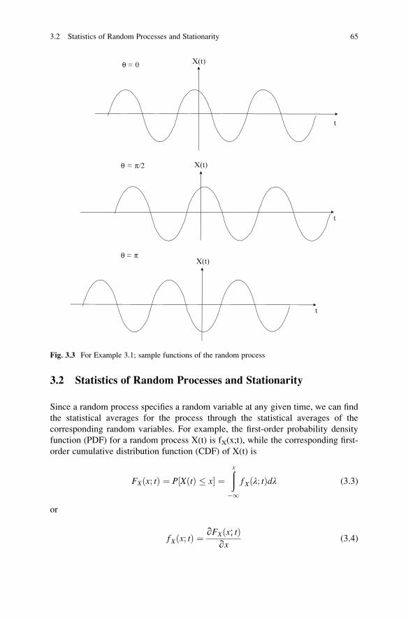
3.2 Statistics of Random Processes and Stationarity

Since a random process specifies a random variable at any given time, we can find

the statistical averages for the process through the statistical averages of the

corresponding random variables. For example, the first-order probability density

function (PDF) for a random process X(t) is fX(x;t), while the corresponding first-

order cumulative distribution function (CDF) of X(t) is

FX x; tð Þ ¼ P X tð Þ � x½ � ¼ðx�1

f X λ; tð Þdλ (3.3)

or

f X x; tð Þ ¼ ∂FX x; tð Þ∂x

(3.4)

θ = 0 X(t)

θ = π/2 X(t)

θ = π

t

t

t

X(t)

Fig. 3.3 For Example 3.1; sample functions of the random process

3.2 Statistics of Random Processes and Stationarity 65

Similarly, if X(t1) ¼ X1 and X(t2) ¼ X2 represent two random variables of a

random process X(t), then their joint distributions are known as second-order PDF

and CDF, which are related as

FX x1; x2; t1; t2ð Þ ¼ P X t1ð Þ � x1,X t2ð Þ � x2½ �

¼ðx2�1

ðx1�1

f X�λ1, λ2; t1, t2

�dλ1dλ2 (3.5)

or

f X x1; x2; t1; t2ð Þ ¼ ∂FX x1; x2; t1; t2ð Þ∂x1∂x2

(3.6)

In general, the joint distributions of n random variables X(t1) ¼ X1, X(t2) ¼ X2,

. . ., X(tn) ¼ Xn provide the nth-order PDF and CDF of a random process X(t) and

are related as

FX x1; x2; . . . ; xn; t1; t2; . . . ; tnð Þ ¼ P X�t1� � x1,X

�t2� � x2, . . . ,X

�tn� � xn

� �¼

ðxn�1

. . .

ðx2�1

ðx1�1

f X�λ1, λ2, . . . , λn; t1, t2, . . . , tn

�dλ1dλ2 . . . dλn

(3.7)

or

f X x1; x2; . . . ; xn; t1; t2; . . . ; tnð Þ ¼ ∂FX x1; x2; . . . ; xn; t1; t2; . . . ; tnð Þ∂x1∂x2 . . .∂xn

(3.8)

A random process X(t) is said to be strictly stationary of order n if its nth-order

PDF and CDF are time-invariant, i.e.

FX x1, x2, . . . , x; t1 þ τ, t2 þ τ, . . . , tn þ τ� �¼ FX x1, x2, . . . , x; t1, t2, . . . , tn

� �(3.9)

i.e. the CDF depends only on the relative location of t1, t2,. . .,tn and not on their

direct values.

We say that {Xk}, k ¼ 0, 1, 2, � � �, n is an independent process if and only if

FX x0; x1; � � �; xn; t0; t1; � � �; tnð Þ ¼ FX0x0; t0ð ÞFX1

x1; t1ð Þ� � �FXnxn; tnð Þ

In addition, if all random variables are drawn from the same distribution, the

process is characterized by a single CDF, FXkxk; tkð Þ, k ¼ 0, 1, 2, � � �, n . In this

case, we call {Xk} a sequence of independent and identically distributed (IID)

random variables.


Having defined the CDF and PDF for a random process X(t), we are now

prepared to define the statistical (or ensemble) averages—the mean, variance,

autocorrelation, and autocovariance of X(t). As in the case of random variables,

these statistics play an important role in practical applications.

The mean or expected value of the random process X(t) is

mX tð Þ ¼ X tð Þ ¼ E X tð Þ½ � ¼ð�1�1

xf X x; tð Þdx (3.10)

where E[•] denotes ensemble average, fX(x;t) is the PDF of X(t) and X(t) is regarded

as a random variable for a fixed value of t. In general, the mean mX(t) is a functionof time.

The variance of a random process X(t) is given by

Var Xð Þ ¼ σ2X ¼ E X tð Þ � mX tð Þð Þ2h i

¼ E X2� �� m2

X (3.11)

The autocorrelation of a random process X(t) is the joint moment of X(t1)

and X(t2), i.e.

RX t1; t2ð Þ ¼ E X t1ð ÞX t2ð Þ½ � ¼ð1�1

ð1�1

x1x2 f X x1; x2; t1; t2ð Þdx1dx2 (3.12)

where fX(x1,x2;t1,t2) is the second-order PDF of X(t). In general, RX(t1,t2) is a

deterministic function of two variables t1 and t2. The autocorrection function is

important because it describes the power-spectral density of a random process.

The covariance or autocovariance of a random process X(t) is the covariance of

X(t1) and X(t2), i.e.

Cov X t1ð Þ,X t2ð Þ½ � ¼ CX t1; t2ð Þ ¼ E X t1ð Þ � mX t1ð Þf g X t2ð Þ � mX t2ð Þf g½ � (3.13a)

Or

Cov X t1ð Þ,X t2ð Þ½ � ¼ RX t1; t2ð Þ � mX t1ð ÞmX t2ð Þ (3.13b)

indicating that the autocovariance can be expressed in terms of the autocorrelation

and the means. Note that the variance of X(t) can be expressed in terms of its

autocovariance, i.e.

Var X tð Þð Þ ¼ CX t; tð Þ (3.14)

The correlation coefficient of a random process X(t) is the correlation coefficient

of X(t1) and X(t2), i.e.


ρX t1; t2ð Þ ¼ CX t1; t2ð ÞffiffiffiffiffiffiffiffiffiffiffiffiffiffiffiffiffiffiffiffiffiffiffiffiffiffiffiffiffiffiffiffiffiffiffiffiCX t1; t1ð ÞCX t2; t2ð Þp (3.15)

where��ρX t1; t2ð Þj � 1.

Finally, we define the nth joint moment of X(t) as

E X t1ð ÞX t2ð Þ . . .X tnð Þ½ �

¼ð1�1

. . .

ð1�1

ð1�1

x1x2 . . . xnf X x1; x2; . . . ; xn; t1; t2; . . . ; tnð Þdx1dx2 . . . dxn(3.16)

We should keep in mind that the mean, variance, autocorrelation,

autocovariance, and nth joint moment are good indicators of the behavior of a

random process but only partial characterizations of the process.

In terms of these statistics, a random process may be classified as follows.

1. A random process is wide-sense stationary (WSS) or weakly stationary if its

mean is constant, i.e.

E X tð Þ½ � ¼ E X t1ð Þ½ � ¼ E X t2ð Þ½ � ¼ mx ¼ constant (3.17)

and its autocorrelation depends only on the absolute time difference

τ ¼ jt1 � t2j, i.e.E X tð ÞX tþ τð Þ½ � ¼ RX τð Þ (3.18)

Note that the autocovariance of a WSS process depends only on the time

difference τ

CX τð Þ ¼ RX τð Þ � m2x (3.19)

and that by setting τ ¼ 0 in Eq. (3.18), we get

E X2 tð Þ� � ¼ RX 0ð Þ (3.20)

indicating that the mean power of a WSS process X(t) does not depend on t. The

autocorrelation function has its maximum value when τ ¼ 0 so that we can write

�RX 0ð Þ � RX τð Þ � RX 0ð Þ (3.21)

2. A random process is said to be strict-sense stationary (SSS) if its statistics are

invariant to shift in the time axis. Hence,

FX x1, x2, . . . , xn; t1 þ τ, t2 þ τ, . . . , tn þ τð Þ¼ FX x1; x2; . . . ; xn; t1; t2; . . . ; tnð Þ (3.22)


An SSS random process is also WSS but the converse is not generally true.

In general terms, a random process is stationary if all its statistical properties do not vary

with time.

Example 3.2 A random process is given by

X tð Þ ¼ A cos ωtþ Θð Þwhere A and ω are constants and Θ is uniformly distributed over (0,2π). (a) Find E

[X(t)] , E[X2(t)] and E[X(t)X(t+τ)]. (b) Is X(t) WSS?

Solution

(a) Since Θ has a uniform distribution, its PDF is given by

f Θ θð Þ ¼1

2π, 0 � θ � 2π

0, otherwise

8<:

Hence,

E X tð Þ½ � ¼ð1�1

xfΘ θð Þdθ ¼ A

ð2π0

cos ωtþ θð Þ 12π

dθ ¼ 0

E X2 tð Þ� � ¼ ð1�1

x2fΘ θð Þdθ ¼ A2

ð2π0

cos 2 ωtþ θð Þ 12π

dθ

¼ A2

ð2π0

1

21þ cos 2 ωtþ θð Þ½ � 1

2πdθ ¼ A2

2

where the trigonometric identity cos 2α ¼ 121þ cos 2α½ � and the fact that

ω ¼ 2π/T have been applied.

E X tð ÞX tþ τð Þ½ ¼ð2π0

A cos ωtþ θð ÞA cos ω tþ τð Þ þ θ½ � 12π

dθ

¼ A2

2π

ð2π0

1

2cos ωτ þ 2ωtþ 2θð Þ þ cosωτ½ �dθ ¼ A2

2cosωτ

where we have used the trigonometric identity cosA cosB ¼12cos Aþ Bð Þ þ cos A� Bð Þ½ �:

(b) Since the mean of X(t) is constant and its autocorrelation is a function of τ only,X(t) is a WSS random process.


Example 3.3 Let X(t) ¼ A sin (πt/2), where A is a Gaussian or normal random

variable with mean μ and variance σ2, i.e. A ¼ N(μ,σ). (a) Determine the mean,

autocorrelation, and autocovariance of X(t). (b) Find the density functions for

X(1) and X(3). (c) Is X(t) stationary in any sense?

Solution

Given that E[A] ¼ μ and Var(A) ¼ σ2, we can obtain

E A2� � ¼ Vax Að Þ þ E2 A½ � ¼ σ2 þ μ2

(a) The mean of X(t) is

mX tð Þ ¼ E A sin πt=2½ � ¼ E A½ � sin πt=2 ¼ μ sin πt=2

The autocorrelation of X(t1) and X(t2) is

RX t1; t2ð Þ ¼ E A sin�πt1=2

�A sin

�πt2=2

�� ¼ E A2� �

sin�πt1=2

�sin

�πt2=2

�¼ σ2 þ μ2ð Þ sin �πt1=2� sin �πt2=2�

The autocovariance is

CX t1; t2ð Þ ¼ RX t1; t2ð Þ � mX t1ð ÞmX t2ð Þ ¼ σ2 sin πt1=2ð Þ sin πt2=2ð Þ(b) X(1) ¼ A sin π(1)/2 ¼ A

FX x1; t1ð Þ ¼ P X 1ð Þ � x1½ � ¼ P A � x1½ � ¼ FA að Þwhere a ¼ x1

f X x1ð Þ ¼ ∂F x1; t1ð Þ∂x1

¼ dFA að Þda

da

dx1¼ f A að Þ

Since A ¼ N(μ,σ),

f A að Þ ¼ 1

σffiffiffiffiffi2πp e� a�μð Þ2= 2σ2ð Þ

f X x1ð Þ ¼ 1

σffiffiffiffiffi2πp e� x1�μð Þ2= 2σ2ð Þ

Similarly, X(3) ¼ A sin π3/2 ¼ �A

FX x3; t1ð Þ ¼ P X 3ð Þ � x3½ � ¼ P �A � x3½ � ¼ P A � �x3½ � ¼ 1� P A � �x3½ �¼ 1� FA að Þ

where a ¼ �x3.


f X x3ð Þ ¼ ∂F x3; t1ð Þ∂x3

¼ dFA að Þda

da

dx3¼ f A að Þ

Hence

f X x3ð Þ ¼ 1

σffiffiffiffiffi2πp e� x3þμð Þ2= 2σ2ð Þ

(c) Since the mean of X(t) is a function of time, the process is not stationary

in any sense.

3.3 Time Averages of Random Processes and Ergodicity

For a random process X(t), we can define two types of averages: ensemble and time

averages. The ensemble averages (or statistical averages) of a random process X

(t) may be regarded as “averages across the process” because they involve all

sample functions of the process observed at a particular instant of time. The time

averages of a random process X(t) may be regarded as “averages along the process”

because they involve long-term sample averaging of the process.

To define the time averages, consider the sample function x(t) of random process

X(t), which is observed within the time interval � T � t � T. The time average(or time mean) of the sample function is

x ¼ < x tð Þ >¼ lim

T !11

2T

ðT�T

x tð Þdt (3.23)

where <•> denotes time-averaging operation. Similarly, the time autocorrelationof the sample function x(t) is given by

R X τð Þ ¼ < x tð Þx tþ τð Þ >¼ lim

T !11

2T

ðT�T

x tð Þx tþ τð Þdt (3.24)

Note that both x and R X τð Þ are random variables since their values depend on

the observation interval and on the sample function x(t) used.

If all time averages are equal to their corresponding ensemble averages, then the

stationary process is ergodic, i.e.

x ¼ < x tð Þ > ¼ E X tð Þ½ � ¼ mX (3.25)

R X τð Þ ¼ < x tð Þx tþ τð Þ > ¼ E X tð ÞX tþ τð Þ½ � ¼ RX τð Þ (3.26)

An ergodic process is one for which time and ensemble averages are interchangeable.

The concept of ergodicity is a very powerful tool and it is always assumed in

many engineering applications. This is due to the fact that it is impractical to have a

3.3 Time Averages of Random Processes and Ergodicity 71

large number of sample functions to work with. Ergodicity suggests that if a random

process is ergodic, only one sample function is necessary to determine the ensemble

averages. This seems reasonable because over infinite time each sample function of

a random process would take on, at one time or another, all the possible values of

the process. We will assume throughout this text that the random processes we will

encounter are ergodic and WSS.

Basic quantities such as dc value, rms value, and average power can be defined

in terms of time averages of an ergodic random process as follows:

1. x ¼ mX is the dc value of x(t).

2. x½ �2 ¼ m2X is the normalized dc power.

3. R X 0ð Þ ¼ x2 is the total average normalized power

4. σ 2X ¼ x2 � x½ �2 is the average normalized power in the ac or time-varying

component of the signal.

5. Xrms ¼ffiffiffiffiffix2

p¼

ffiffiffiffiffiffiffiffiffiffiffiffiffiffiffiffiffiffiffiffiσ 2X þ x½ �2

qis the rms value of x(t).

Example 3.4 Consider the random process in Example 3.2. Show that the process is

stationary and ergodic.

Solution

We already showed that the process is stationary because the statistical or ensemble

averages do not depend on time. To show that the process is ergodic, we compute

the first and second moments. Since ω ¼ 2π/T,

x ¼ lim

T !11

2T

ðT�T

A cos ωtþ θð Þdt ¼ 0

x2 ¼ lim

T !11

2T

ðT�T

A2 cos 2 ωtþ θð Þdt ¼ lim

T !1A2

2T

ðT�T

1

21þ cos 2 ωtþ θð Þ½ �dt ¼ A2

2

indicating that the time averages are equal to the ensemble averages we obtained in

Example 3.2. Hence the process is ergodic.

3.4 Multiple Random Processes

The joint behavior of two or more random processes is dictated by their joint

distributions. For example, two random processes X(t) and Y(t) are said to be

independent if for all t1 and t2, the random variables X(t1) and Y(t2) are indepen-

dent. That means that their nth order joint PDF factors, i.e.

FXY x1; y1; x2; y2; . . . ; xn; yn; t1; t2; . . . ; tnð Þ¼ FX x1; x2; . . . ; xn; t1; t2; . . . ; tnð ÞFY y1; y2; . . . ; yn; t1; t2; . . . ; tnð Þ (3.27)


The crosscorreleration between two random processes X(t) and Y(t) is

defined as

RXY t1; t2ð Þ ¼ E X t1ð ÞY t2ð Þ½ � (3.28)

Note that

RXY t1; t2ð Þ ¼ RYX t2; t1ð Þ (3.29)

The processes X(t) and Y(t) are said to be orthogonal if

RXY t1; t2ð Þ ¼ 0 for all t1 and t2 (3.30)

If X(t) and Y(t) are jointly stationary, then their crosscorrelation function

becomes

RXY t1; t2ð Þ ¼ RXY τð Þwhere τ ¼ t2 � t1. Other properties of the crosscorrelation of jointly stationary

processes are:

1. RXY(�τ) ¼ RXY(τ), i.e. it is symmetric.

2.��RXY τð Þj � ffiffiffiffiffiffiffiffiffiffiffiffiffiffiffiffiffiffiffiffiffiffiffi

RX 0ð ÞRY 0ð Þp, i.e. it is bounded.

3. RXY τð Þ�� 12RX 0ð Þ þ RY 0ð Þ½ �� , i.e. it is bounded.

The crosscovariance of X(t) and Y(t) is given by

CXY t1; t2ð Þ ¼ E X t1ð Þ � mX t1ð Þf g Y t2ð Þ � mY t2ð Þf g½ � ¼ RXY t1; t2ð Þ � mX t1ð ÞmY t2ð Þ(3.31)

Just like with random variables, two random processes X(t) and Y(t) are uncor-related if

CXY t1; t2ð Þ ¼ 0 for all t1 and t2 (3.32)

which implies that

RXY t1; t2ð Þ ¼ mX t1ð ÞmY t2ð Þ for all t1 and t2 (3.33)

Finally, for jointly ergodic random processes X(t) and Y(t),

R XY τð Þ ¼ lim

T !11

2T

ðT�Tx tð Þx tþ τð Þdt ¼ RXY τð Þ (3.34)

Thus, two random processes X(t) and Y(t) are:

(a) Independent if their joint PDF factors.

(b) Orthogonal if RXY(t1,t2) ¼ 0 for all t1 and t2(c) Uncorrelated if RXY(t1,t2) ¼ mX(t1)mY(t2) for all t1 and t2.

3.4 Multiple Random Processes 73

Example 3.5 Two random processes are given by

X tð Þ ¼ sin ωtþ Θð Þ, Y tð Þ ¼ sin ωtþ Θþ π=4ð Þwhere Θ is random variable that is uniformly distributed over (0,2π). Find the crosscorrelation function RXY(t,t + τ)

Solution

RXY t, tþ τð Þ ¼ RXY

�τ� ¼ E X

�t�Y�tþ τ

�� ¼ ð2π0

x tð Þy tþ τð ÞfΘ θð Þdθ

¼ð2π0

sin ωtþ θð Þ sin ω tþ τð Þ þ θ þ π=4½ � 12π

dθ

¼ð2π0

1

2cos ωτ þ π=4ð Þ � cos

�2ωtþ ωτ þ 2θ þ π=4

� � 1

2πdθ

¼ 1

2cos ωτ þ π=4ð Þ

where we have applied the trigonometric identity sinA sinB ¼12cos A� Bð Þ � cos Aþ Bð Þ½ �.

Example 3.6 A received signal X(t) consists of two components: desired signal

S(t) and noise N(t), i.e.

X(t) ¼ S(t) + N(t)

If the autocorrelation of the random signal is

RS τð Þ ¼ e�2jτj

while that of the random noise is

RN τð Þ ¼ 3e�jτj

Assume that they are independent and they both have zero mean.

(a) Find the autocorrelation of X(t). (b) Determine the cross correlation between

X(t) and S(t).

Solution

(a) RX t1; t2ð Þ ¼ E X�t1�X�t2�� ¼ E S t1ð Þ þ N t1ð Þf g S t2ð Þ þ N t2ð Þf g½ �

¼ E S t1ð ÞS�t2�� þ E N

�t1�S�t2�� þ E S

�t1�N�t2�� þ E N

�t1�N�t2��

Since S(t) and N(t) are independent and have zero mean,


E N t1ð ÞS t2ð Þ½ � ¼ E N t1ð Þ½ �E S t2ð Þ½ � ¼ 0

E S t1ð ÞN t2ð Þ½ � ¼ E S t1ð Þ½ �E N t2ð Þ½ � ¼ 0

Hence,

RX τð Þ ¼ RS τð Þ þ RN τð Þ ¼ e�2jτj þ 3e�jτj

where τ ¼ t1 � t2.

(b) Similarly,

RXS t1; t2ð Þ ¼ E X�t1�S�t2�� ¼ E S t1ð Þ þ N t1ð Þf g S t2ð Þf g½ �

¼ E S t1ð ÞS�t2�� þ E N

�t1�S�t2��

¼ RS t1; t2ð Þ þ 0

Thus,

RXS τð Þ ¼ RS τð Þ ¼ e�2jτj

3.5 Sample Random Processes

We have been discussing random processes in general. Specific random processes

include Poisson counting process, Wiener process or Brownian motion, random

walking process, Bernoulli process, birth-and-death process, and Markov process

[4, 5]. In this section, we consider some of these specific random processes.

3.5.1 Random Walks

A random walk (or drunkard’s walk) is a stochastic process in which the states are

integers Xn representing the position of a particle at time n. Each state change

according to

Xn ¼ Xn�1 þ Zn (3.35)

where Zn is a random variable which takes values of 1 or �1. If X0 ¼ 0, then

Xn ¼Xni¼1

Zi (3.36)

A random walk on X corresponds to a sequence of states, one for each step of the

walk. At each step, the walk switches from its current state to a new state or remains

at the current state. Thus,

3.5 Sample Random Processes 75

Random walks constitute a random process consisting of a sequence of discrete steps of

fixed length.

Random walks are usually Markovian, which means that the transition at each

step is independent of the previous steps and depends only on the current state.

Although random walks are not limited to one-dimensional problems, the

one-dimensional random walk is one of the simplest stochastic processes and can

be used to model many gambling games. Random walks also find applications in

potential theory. A typical one-dimensional random walk is illustrated in Fig. 3.4.

Example 3.7 Consider the following standard Markovian random walk on the

integers over the range {0, . . ., N} that models a simple gambling game, where a

player bets the same amount on each hand (i.e., step). We assume that if the player

ever reaches 0, he has lost all his money and stops, but if he reaches N, he has won acertain amount of money and stops. Otherwise, at each step, one moves from state

i (where i 6¼ 0, N) to i + 1 with probability p (the probability of winning the game),

to i � 1 with probability q (the probability of losing the game), and stays at the

same state with probability 1 � p � q (the probability of a draw).

3.5.2 Markov Processes

If the future state of a process depends only on the present (and independent of the

past), the process is called a Markov process. A Markov process is made possible

only if the state time has a memoryless (exponential) distribution. This requirement

often limits the applicability of Markov processes.

Formally, a stochastic process X(t) is a Markov process if

Prob X tð Þ ¼ x��X tnð Þ ¼ xn,X tn�1ð Þ ¼ xn�1� � �,X toð Þ ¼ xo

� �¼ Prob X tð Þ ¼ x

��X tnð Þ ¼ xn� �

for to < t1 < � � � < tn < t (3.37)

A discrete-state Markov process is called a Markov chain [4]. We use the state

transition diagram to represent the evolution of a Markov chain. An example of

three-state Markov chain is shown in Fig. 3.5.

p pp

qq q

n-1 n n+1

Fig. 3.4 A typical

random walk


The conditional probability

Prob Xnþ1 ¼ i��Xn ¼ j

� � ¼ pn i; jð Þis called the transition probability from state i to state j. Since a Markov chain must

go somewhere with a probability of 1, the sum of pn(i,j)’s over all j’s is equal to 1. If

pn(i,j) is independent of n, the Markov chain is said to be time-homogeneous and in

this case, the transition probability becomes p(i,j). When we arrange p(i,j) into an

square array, the resulting matrix is called the transition matrix.For a simple example, consider four possible states as 0, 1, 2, and 3. The

transition matrix is

P ¼p 0; 0ð Þ p 0; 1ð Þ p 0; 2ð Þ p 0; 3ð Þp 1; 0ð Þ p 1; 1ð Þ p 1; 2ð Þ p 1; 3ð Þp 2; 0ð Þ p 2; 1ð Þ p 2; 2ð Þ p 2; 3ð Þp 3; 0ð Þ p 3; 1ð Þ p 3; 2ð Þ p 3; 3ð Þ

2664

3775 (3.38)

3.5.3 Birth-and-Death Processes

Birth-death processes describe the stochastic evolution in time of a random variable

whose value increases or decreases by one in a single event. These are discrete-

space Markov processes in which the transitions are restricted to neighboring states

only. A typical example is shown in Fig. 3.6.

For example, the number of jobs in a queue with a single server and the

individual arrivals can be represented as a birth-death process. An arrival to the

queue (a birth) causes the state to change by +1, while a departure (a death) causes

the state to change by �1. Although the birth-death processes are used in modeling

population, they are useful in the analysis of communication networks. They are

also used in physics, biology, sociology, and economics.

1 20

p00

p02

p20

p10 p21

p22

p11

p12p01

Fig. 3.5 State transition

diagram for a three-state

Markov chain


3.5.4 Poisson Processes

From application point of view, Poisson processes are very useful. They can be used

to model a large class of stochastic phenomena. Poisson process is one in which the

number of events which occur in any time interval t is distributed according to a

Poisson random variable, with mean λt. In this process, the interarrival time is

distributed exponentially.

A process is called a Poisson process when the time intervals between successive events

are exponentially distributed.

Given a sequence of discrete events occurring at times t0, t1, t2, t3,. . ., the intervalsbetween successive events areΔt1 ¼ (t1 � t0),Δt2 ¼ (t2 � t1),Δt3 ¼ (t3 � t2), . . .,and so on. For a Poisson process, these intervals are treated as independent random

variables drawn from an exponentially distributed population, i.e., a population with

the density function f(x) ¼ λe�λ x for some fixed constant λ. The interoccurrence

times between successive events of a Poisson process with parameter λ are indepen-dent identical distributed (IID) exponential random variable with mean 1/λ.

The Poisson process is a counting process for the number of randomly occurring

point-events observed in a given time interval. For example, suppose the arrival

process has a Poisson type distribution. If N(t) denotes the number of arrivals in

time interval (0,t], the probability mass function for N(t) is

pn tð Þ ¼ P N tð Þ ¼ n½ � ¼ λtð Þnn!

e�λt (3.39)

Thus, the number of events N(t) in the interval (0,t] has a Poisson distribution

with parameter λt and the parameter λ is called the arrival rate of the Poisson

process.

Two properties of the Poisson process are the superposition property and

decomposition property [6, 7].

The superposition (additive) property states that the superposition of Poisson

processes is also a Poisson process, as illustrated in Fig. 3.7.

Thus, the sum of n independent Poisson processes with parameters λk, k ¼ 1, 2,

� � �, n is a Poisson process with parameter λ ¼ λ1 þ λ2 þ � � � þ λn.The decomposition (splitting) property is just the reverse of the superposition

property. If a Poisson stream is split into k substreams, each substream is also

Poisson, as illustrated in Fig. 3.8.

λ λ λ λ

μ μ μ μ

1. . .

n-10 n n+1

Fig. 3.6 The state transition diagram for a birth-and-death process


The Poisson process is related to the exponential distribution. If the interarrival

times are exponentially distributed, the number of arrival-points in a time interval is

given by the Poisson distribution and the process is a Poisson arrival process. The

converse is also true—if the number of arrival-points in any interval is a Poisson

process, the interarrival times are exponentially distributed.

The relationship among various types of stochastic processes is shown in Fig. 3.9.

λ

λ1

λ2

λ3

λN

⋅⋅

Fig. 3.7 Superposition of

Poisson streams

p1lp1

p2 p2lλ

p3 p3l

pN

pNl

⋅

⋅

Fig. 3.8 Decomposition of

a Poisson stream

Poisson Processes

Birth-death Processes

Markov Processes


between various types of

stochastic processes


3.6 Renewal Processes

A renewal process generalizes the notion of a Markov process. In a Markov process,

the times between state transitions are exponentially distributed. Let X1, X2, X3, � � �be times of successive occurrences of some phenomenon and let Zi ¼ Xi � Xi � 1

be the times between (i � 1th) and ith occurrences, then if {Zi} are independent andidentically distributed (IID), the process {Xi} is called a renewal process. The studyof renewal processes is called renewal theory.

One common example of a renewal process is the arrival process to a queueing

system. The times between successive arrivals are IID. In a special case that the

interarrival times are exponential, the nenewal process is a Poisson process. Poisson

process, binomial process, and random walk process are special cases of renewal

processes.

3.7 Computation Using MATLAB

The MATLAB software can be used to reinforce the concepts learned in this

chapter. It can be used to generate a random process X(t) and calculate its statistics.

It can also be used to plot X(t) and its autocorrelation function.

MATLAB provides command rand for generating uniformly distributed ran-

dom numbers between 0 and 1. The uniform random number generator can then be

used to generate a random process or the PDF of an arbitrary random variable. For

example, to generate a random variable X uniformly distributed over (a,b), we use

X ¼ aþ a� bð ÞU (3.40)

where U is generated by rand. A similar command randn generates a Gaussian

(or normal) distribution with mean zero and variance one.

Suppose we are interested in generating a random process

X tð Þ ¼ 10 cos 2πtþ Θð Þ (3.41)

where Θ is a random variable uniformly distributed over (0,2π). We generate and

plot X(t) using the following MATLAB commands.

» t¼0:0.01:2; % select 201 time points between 0 and 2.» n¼length(t);» theta¼2*pi*rand(1,n); % generates n¼201 uniformly

distributed theta» x¼10*cos(2*pi*t +theta);» plot(t,x)

The plot of the random process is shown in Fig. 3.10.


Wemay find the mean and standard deviation using MATLAB commandsmean

and std respectively. For example, the standard deviation is found using

» std(x)ans ¼

7.1174

where the result is a bit off from the exact value of 7.0711 obtained from Example

3.2. The reason for this discrepancy is that we selected only 201 points. If more

points, say 10,000, are selected the two results should be very close.

We will now use MATLAB to generate a Bernoulli random process, which is

used in data communication. The process consists of random variables which

assume only two states or values: +1 and �1 (or +1 and 0). In this particular

case, the process may also be regarded as random binary process. The probabilityof X(t) being +1 is p and �1 is q ¼ 1 � p. Therefore, to generate a Bernoulli

random variable X, we first use MATLAB rand to generate a random variable U

that uniformly distributed over (0,1). Then, we obtain

X ¼ 1, if U � p�1, if U > p

�(3.42)

i.e. we have partitioned the interval (0,1) into two segments of length p and 1 � p.

The following MATLAB program is used to generate a sample function for the

random process. The sample function is shown in Fig. 3.11.

0 0.2 0.4 0.6 0.8 1 1.2 1.4 1.6 1.8 2-10

-8

-6

-4

-2

0

2

4

6

8

10

Fig. 3.10 MATLAB generation of the random process X(t) ¼ 10 cos(2πt + Θ)


% Generation of a Bernoulli process% Ref: D. G. Childers, "Probability of Random Processes,"

Irwin, 1997, p.164p¼0.6; % probability of having +1q¼1-p; % probability of having -1n¼30; % length of the discrete sequencet¼rand(1,n); % generate random numbers uniformly

distributed over (0,1)x¼zeros(length(t)); % set initial value of x equal to zerofor k¼1:n

if( t(k) <¼ p )x(k)¼1;

elsex(k)¼ -1;

endendstairs(x);xlabel(’t’)ylabel(’x(t)’)a¼axis;axis([a(1) a(2) -2 2]);grid on

Fig. 3.11 A typical sample function of a Bernoulli random process


3.8 Summary

1. A random process (also known as stochastic process) is a mapping from the

sample space into an ensemble of time functions known as sample functions.

At any instant of time, the value of a random process is a random variable.

2. A continuous-time random process X(t) is a family of sample functions of

continuous random variables that are a function of time t, where t is a continuum

of values. A random process is deterministic if future values of any sample

function can be predicted from past values.

3. A random process is stationary if all its statistical properties does not change

with time, i.e mX(t) is constant and RX(t1,t2) depends only on τ ¼ jt2 � t1j.4. For an ergodic process, the statistical and time averages are the same and only

one sample function is needed to compute ensemble averages.

5. For two stationary random processes X(t) and Y(t), the cross-correlation func-

tion is defined as

RXY τð Þ ¼ E X tð ÞY tþ τð Þ½ �Widely used random processes in communication include random walk,

birth-and-death process, Poisson process, Markov process, and renewal process.

6. Some of the concepts covered in the chapter are demonstrated using MATLAB.

For more information on the material covered in this chapter, one should

see [8–10].

Problems

3.1 If X(t) ¼ A sin4t, where A is random variable uniformly distributed between

0 and 2, find E[X(t)] and E[X2(t)].

3.2 Given a random process X(t) ¼ At + 2, where A is a random variable uni-

formly distributed over the range (0,1),

(a) sketch three sample functions of X(t),

(b) find X tð Þ and X2 tð Þ ,(c) determine RX(t1,t2),(d) Is X(t) WSS?

3.3 If a random process is given by

X tð Þ ¼ A cosωt� B sinωt,

where ω is a constant and A and B are independent Gaussian random variables

with zero mean and variance σ2, determine: (a) E[X], E[X2] and Var(X),

(b) the autocorrelation function RX(t1,t2).

Problems 83

3.4 Let Y(t) ¼ X(t � 1) + cos3t, where X(t) is a stationary random process.

Determine the autocorrelation function of Y(t) in terms of RX(τ).3.5 If Y(t) ¼ X(t) � X(t � α), where α is a constant and X(t) is a random

process. Show that

RY t1; t2ð Þ ¼ Rx t1; t2ð Þ � Rx t1, t2 � αð Þ � Rx t1 � α, t2ð Þ þ Rx t1 � α, t2 � αð Þ3.6 A random stationary process X(t) has mean 4 and autocorrelation functon

RX τð Þ ¼ 5e�2jτj

(a) If Y(t) ¼ X(t � 1), find the mean and autocorrelation function of Y(t).

(b) Repeat part (a) if Y(t) ¼ tX(t).

3.7 Let Z(t) ¼ X(t) + Y(t), where X(t) and Y(t) are two independent stationary

random processes. Find RZ(τ) in terms of RX(τ) and RY(τ).3.8 Repeat the previous problem if Z(t) ¼ 3X(t) + 4Y(t).

3.9 If X(t) ¼ Acosωt, where ω is a constant and A random variables with mean μand variance σ2, (a) find < x(t) > and mX(t). (b) Is X(t) ergodic?

3.10 A random process is defined by

X tð Þ ¼ A cosωt� B sinωt,

where ω is a constant and A and B are independent random variable with zero

mean. Show that X(t) is stationary and also ergodic.

3.11 N(t) is a stationary noise process with zero mean and autocorrelation function

RN τð Þ ¼ No

2δ τð Þ

where No is a constant. Is N(t) ergodic?

3.12 X(t) is a stationary Gaussian process with zero mean and autocorrelation

function

RX τð Þ ¼ σ2e�αjτj cosωτ

where σ, ω, and α are constants. Show that X(t) is ergodic.

3.13 If X(t) and Y(t) are two random processes that are jointly stationary so that

RXY(t1,t2) ¼ RXY(τ), prove that

RXY τð Þ ¼ RYX �τð Þwhere τ ¼ jt2 � t1j.

3.14 For two stationary processes X(t) and Y(t), show that


(a)��RXY τð Þj � 1

2RX 0ð Þ þ RY 0ð Þ½ �

(b)��RXY τð Þj �

ffiffiffiffiffiffiffiffiffiffiffiffiffiffiffiffiffiffiffiffiffiffiffiRX 0ð ÞRY 0ð Þ

p3.15 Let X(t) and Y(t) be two random processes given by

X(t) ¼ cos (ωtþΘ)Y(t) ¼ sin (ωtþΘ)

where ω is a constant and Θ is a random variable uniformly distributed over

(0,2π). Find

RXY t, tþ τð Þ and RYX t, tþ τð Þ:3.16 X(t) and Y(t) are two random processes described as

X(t) ¼ A cos ωt + B sin ωtY(t) ¼ B cos ωt � A sin ωt

where ω is a constant and A ¼ N(0,σ2) and B ¼ N(0,σ2). Find RXY(τ).3.17 Let X(t) be a stationary random process and Y(t) ¼ X(t) � X(t � a), where a

is a constant. Find RXY(τ).3.18 Let N tð Þ, t � 0f g be a Poisson process with rate λ. Find E N tð Þ:N tþ sð Þ½ �.3.19 For a Poisson process, show that if s < t,

Prob N sð Þ ¼ k��N tð Þ ¼ n

� � ¼ nk

s

t

� �k1� s

t

� �n�k, k ¼ 0, 1, � � �, n

3.20 Let N(t) be a renewal process where renewal epochs are Erlang with

parameters (m,λ). Show that

Prob N tð Þ ¼ n½ � ¼Xnmþm�1

k¼nm

λtð Þkk!

e�λt

3.21 Use MATLAB to generate a random process X(t) ¼ A cos(2πt), where A is a

Gaussian random variable with mean zero and variance one. Take

0 < t < 4 s.

3.22 Repeat the previous problem if A is random variable uniformly distributed

over (�2, 2).3.23 Given that the autocorrelation function RX τð Þ ¼ 2þ 3e�τ

2

, use MATLAB to

plot the function for �2 < τ < 2.

3.24 Use MATLAB to generate a random process

Problems 85

X tð Þ ¼ 2 cos 2πtþ B n½ � π4

� �where B[n] is a Bernoulli random sequence taking the values of +1 and �1.Take 0 < t < 3 s.

References

1. X. R. Li, Probability, Random Signals, and Statistics. Boca Raton, FL: CRC Press, 1999,

pp. 259-313.

2. G. R. Grimmett and D. R. Stirzaker, Probability and Random Processes. New York: Oxford

University Press, 3rd ed., 2001, pp. 360-374.


Verlag, 1995, pp. 235-282.

4. D. Claiborne, Mathematical Preliminaries for Computer Networking. New York: John Wiley

& Sons, 1990, pp. 35-42.

5. S. M. Ross, Stochastic Processes. New York: John Wiley & Sons, 1983.

6. R. Jain, The Art of Computer Systems Performance Analysis. New York: John Wiley, 1991,

pp. 516-517.

7. J. Medhi, Stochastic Models in Queueing Theory. Boston, MA: Academic Press, 1991, p. 31.

8. R. Goodman, Introduction to Stochastic Models. Mineola, NY: Dover Publications, 2nd ed.,

2006.

9. O. C. Ibe, Fundamentals of Applied Probability and Random Processes. Burlington, MA:

Elsevier Academic Press, 2005.

10. J. C. Falmagne, Lectures in Elementary Probability Theory and Stochastic Processes. NewYork: McGraw-Hill, 2003.


Chapter 4

Queueing Theory

The priest persuades humble people to endure their hard lot,a politician urges them to rebel against it, and a scientistthinks of a method that does away with the hard lotaltogether.

—Max Percy

Queueing is simply waiting in lines such as stopping at the toll booth, waiting in line

for a bank cashier, stopping at a traffic light, waiting to buy stamps at the post office,

and so on.

A queue consists of a line of people or things waiting to be served and a service center with

one or more servers.

For example, there would be no need of queueing in a bank if there are infinite

number of people serving the customers. But that would be very expensive and

impractical.

Queueing theory is applied in several disciplines such as computer systems,

traffic management, operations, production, and manufacturing. It plays a signifi-

cant role in modeling computer communication networks. Since the mid-1960s

performance evaluation of computer communication systems are usually made

using queueing models.

Reduced to its most basic form, a computer network consists of communica-

tion channels and processors (or nodes). As messages flow from node to node,

queues begin to form different nodes. For high traffic intensity, the waiting or

queueing time can be dominant so that the performance of the network is dictated

by the behavior of the queues at the nodes. Analytical derivation of the waiting

time requires a knowledge of queueing theory. Providing the basic fundamentals

of queueing theory needed for the rest of the book will be our objective in

this chapter.


87

4.1 Kendall’s Notation

In view of the complexity of a data network, we first examine the properties of a

single queue. The results from a single queue model can be extended to model a

network of queues. A single queue is comprised of one or more servers and

customers waiting for service. As shown in Fig. 4.1, the queue is characterized by

three quantities:

• the input process,

• the service mechanism, and

• the queue discipline.

The input process is expressed in terms of the probability distribution of the

interarrival times of arriving customers. The service mechanism describes the

statistical properties of the service process. The queue discipline is the rule used

to determine how the customers waiting get served. To avoid ambiguity in

specifying these characteristics, a queue is usually described in terms of a well-

known shorthand notation devised by D. G. Kendall [1]. In Kendall’s notation,

a queue is characterized by six parameters as follows:

A=B=C=K=m=z (4.1)

where the letters denote:

A: Arrival process, i.e. the interarrival time distribution

B: Service process, i.e. the service time distribution

C: Number of servers

K: Maximum capacity of the queue (default ¼ 1)

m: Population of customers (default ¼ 1)

z: Service discipline (default ¼ FIFO)

The letters A and B represent the arrival and service processes and assume the

following specific letters depending on which probability distribution law is

adopted:

D: Constant (deterministic) law, i.e. interarrival/service times are fixed

M: Markov or exponential law, i.e. interarrival/service times are exponentially

distributed

G: General law, i.e. nothing is known about the interarrival/service time distribution

Arrival rate Departure rate

Queue Server

Fig. 4.1 A typical queueing system

88 4 Queueing Theory

GI: General independent law, i.e. all interarrival/service times are independent

Ek: Erlang’s law of order k

Hk: Hyperexponential law of order k

The most commonly used service disciplines are:

FIFO: first-in first-out

FCFS: first-come first-serve

LIFO: last-in first-out

FIRO: first-in random-out.

It is common in practice to represent a queue by specifying only the first three

symbols of Kendall’s notation. In this case, it is assumed that K ¼ 1, m ¼ 1, and

z ¼ FIFO. Thus, for example, the notation M/M/1 represents a queue in which

arrival times are exponentially distributed, service times are exponentially

distributed, there is one server, the queue length is infinite, the customer population

is infinite, and the service discipline is FIFO. In the same way, an M/G/n queue is

one with Poisson arrivals, general service distribution, and n servers.

Example 4.1 A single-queue system is denoted by M/G/4/10/200/FCFS. Explain

what the operation of the system is.

Solution

The system can be described as follows:

1. The interval arrival times is exponentially distributed.

2. The services times follow a general probability distribution.

3. There are four servers.

4. The buffer size of the queue is 10.

5. The population of customers to be served is 200, i.e. only 200 customers can

occupy this queue.

6. The service discipline is first come, first served.

4.2 Little’s Theorem

To obtain the waiting or queueing time, we apply a useful result, known as Little’stheorem after the author of the first formal proof in 1961. The theorem relates the

mean number of customers in a queue to the mean arrival rate and the mean waiting

time. It states that a queueing system, with average arrival rate λ and mean waiting

time per customer E(W), has a mean number of customers in the queue (or average

queue length) E(Nq) given by

E Nq

� � ¼ λE Wð Þ (4.2)

The theorem is very general and applies to all kinds of queueing systems. It

assumes that the system is in statistical equilibrium or steady state, meaning that the

4.2 Little’s Theorem 89

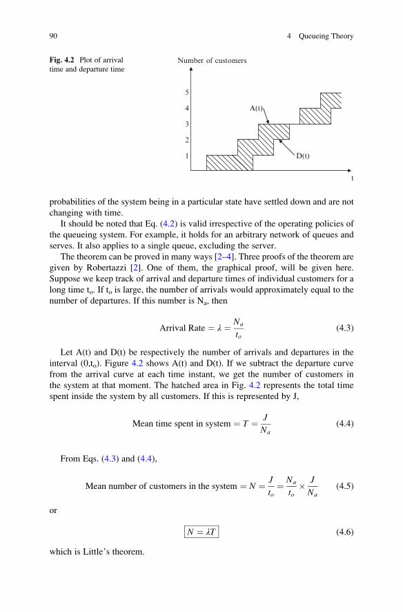
probabilities of the system being in a particular state have settled down and are not

changing with time.

It should be noted that Eq. (4.2) is valid irrespective of the operating policies of

the queueing system. For example, it holds for an arbitrary network of queues and

serves. It also applies to a single queue, excluding the server.

The theorem can be proved in many ways [2–4]. Three proofs of the theorem are

given by Robertazzi [2]. One of them, the graphical proof, will be given here.

Suppose we keep track of arrival and departure times of individual customers for a

long time to. If to is large, the number of arrivals would approximately equal to the

number of departures. If this number is Na, then

Arrival Rate ¼ λ ¼ Na

to(4.3)

Let A(t) and D(t) be respectively the number of arrivals and departures in the

interval (0,to). Figure 4.2 shows A(t) and D(t). If we subtract the departure curve

from the arrival curve at each time instant, we get the number of customers in

the system at that moment. The hatched area in Fig. 4.2 represents the total time

spent inside the system by all customers. If this is represented by J,

Mean time spent in system ¼ T ¼ J

Na(4.4)

From Eqs. (4.3) and (4.4),

Mean number of customers in the system ¼ N ¼ J

to¼ Na

to� J

Na(4.5)

or

N ¼ λT (4.6)

which is Little’s theorem.

Number of customers

5

4 A(t)

3

2

1 D(t)

t

Fig. 4.2 Plot of arrival

time and departure time


4.3 M/M/1 Queue

Consider the M/M/1 queue shown in Fig. 4.3.

This is a single-server system with infinite queue size, Poisson arrival process

with arrival rate λ, and exponentially distributed service times with service rate μ.The queue discipline is FCFS.

The probability of k arrivals in a time interval t is given by the Poisson

distribution:

p kð Þ ¼ λtð Þkk!

e�λt, k ¼ 0, 1, 2, � � � (4.7)

(Note that the Poisson arrival process has exponential arrival times.) It is readily

shown that the mean or expected value and variance are given by

E kð Þ ¼X1k¼0

kp kð Þ ¼ λt (4.8a)

Var kð Þ ¼ E k � E kð Þð Þ2h i

¼ λt (4.8b)

One way of analyzing such a queue is to consider its state diagram [5–8] in

Fig. 4.4.

Infinite buffer

Poisson arrivals, λ

Fig. 4.3 M/M/1 queue

. ..

μ

0 12

n-1

μ μ

n+1

μ

λ λ λ λ

n. . .

Fig. 4.4 State diagram for M/M/1 queue

4.3 M/M/1 Queue 91

We say that the system is in state n where there are n customers in the system

(in the queue and the server). Notice from Fig. 4.4 that λ is the rate of moving from

state n to n+1 due to an arrival in the system, whereas μ is the rate of moving

from state n to n � 1 due to departure when service is completed. If N(t) is

the number of customers in the system (in the queue and the server) at time t,

the probability of the queue being in state n at steady state is given by

pn ¼ limt!1 Prob N tð Þ ¼ n½ �, n ¼ 0, 1, 2, � � � (4.9)

Our goal is to find pn and use it to find some performance measures of interest.

Consider when the system is in state 0. Due to an arrival, the rate at which the

process leaves state 0 for state 1 is λpo. Due to a departure, the rate at which

the process leaves state 1 for state 0 is μp1. In order for stationary probability to

exist, the rate of leaving state 0 must equal the rate of entering it. Thus

λpo ¼ μp1 (4.10)

When the system is in state 1. Since p1 is the proportion of time the system is in

state 1, the total rate at which arrival or departure occurs is λp1 + μp1, which is the

rate at which the process leaves state 1. Similarly, the total rate at which the process

enters state 1 is λp0 + μp2. Applying the rate-equality principle gives

λp1 þ μp1 ¼ λp0 þ μp2 (4.11)

We proceed in this manner for the general case of the system being in state n and

obtain

λþ μð Þpn ¼ λpn�1 þ μpnþ1, n � 1 (4.12)

The right-hand side of this equation denotes the rate of entering state n, while the

left-hand side represents the rate of leaving state n. Equations (4.10–4.12) are called

balance equations.We can solve Eq. (4.12) in several ways. An easy way is to write Eq. (4.12) as

λpn � μpnþ1 ¼ λpn�1 � μpn¼ λpn�2 � μpn�1¼ λpn�3 � μpn�2⋮ ⋮¼ λp0 � μp1 ¼ 0

(4.13)

Thus

λpn ¼ μpnþ1 (4.14)

or

pnþ1 ¼ ρpn, ρ ¼ λ=μ (4.15)


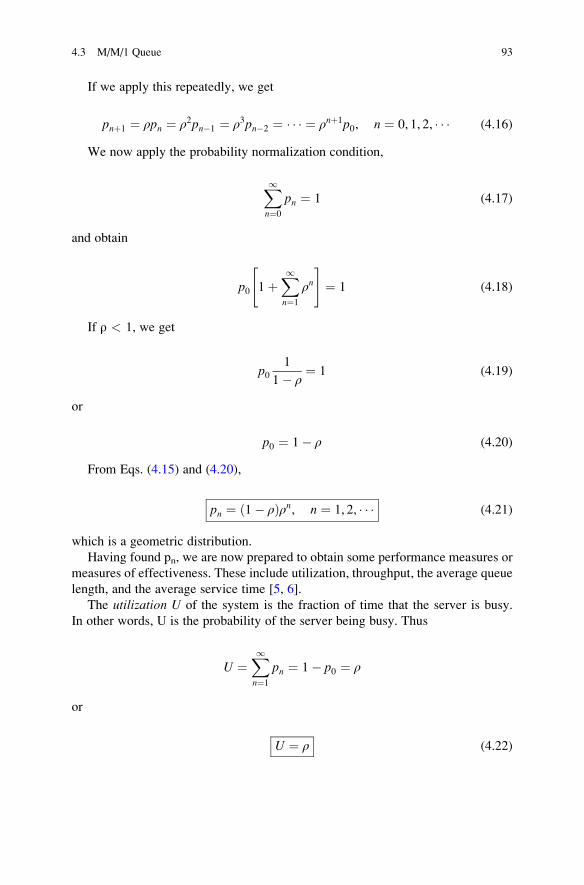
If we apply this repeatedly, we get

pnþ1 ¼ ρpn ¼ ρ2pn�1 ¼ ρ3pn�2 ¼ � � � ¼ ρnþ1p0, n ¼ 0, 1, 2, � � � (4.16)

We now apply the probability normalization condition,

X1n¼0

pn ¼ 1 (4.17)

and obtain

p0 1þX1n¼1

ρn" #

¼ 1 (4.18)

If ρ < 1, we get

p01

1� ρ¼ 1 (4.19)

or

p0 ¼ 1� ρ (4.20)

From Eqs. (4.15) and (4.20),

pn ¼ 1� ρð Þρn, n ¼ 1, 2, � � � (4.21)

which is a geometric distribution.

Having found pn, we are now prepared to obtain some performance measures or

measures of effectiveness. These include utilization, throughput, the average queue

length, and the average service time [5, 6].

The utilization U of the system is the fraction of time that the server is busy.

In other words, U is the probability of the server being busy. Thus

U ¼X1n¼1

pn ¼ 1� p0 ¼ ρ

or

U ¼ ρ (4.22)

4.3 M/M/1 Queue 93

The throughput R of the system is the rate at which customers leave the queue

after service, i.e. the departure rate of the server. Thus

R ¼ μ 1� p0ð Þ ¼ μρ ¼ λ (4.23)

This should be expected because the arrival and departure rates are equal at

steady state for the system to be stable.

The average number of customers in the system is

E Nð Þ ¼X1n¼0

npn ¼X1n¼0

n 1� ρð Þρn ¼ 1� ρð ÞX1n¼0

nρn

¼ 1� ρð Þ ρ

1� ρð Þ2

or

E Nð Þ ¼ ρ

1� ρ(4.24)

Applying Little’s formula, we obtain the average response time or averagedelay as

E Tð Þ ¼ E Nð Þλ¼ 1

λ

ρ

1� ρ(4.25)

or

E Tð Þ ¼ 1

μ 1� ρð Þ (4.26)

This is the mean value of the total time spent in the system (i.e. queue and the

server).

As shown in Fig. 4.5, the average delay E(T) is the sum of the average waiting

time E(W) and the average service time E(S), i.e.

E Tð Þ ¼ E Wð Þ þ E Sð Þ (4.27)

Equivalently, the average number of customers E(N) in the system equals the

sum of the average of customers waiting E(Nq) in the queue and the average number

of customers E(Ns) being served, i.e.

E Nð Þ ¼ E Nq

� �þ E Nsð Þ (4.28)


But the mean service E Sð Þ ¼ 1μ. Thus

E Wð Þ ¼ E Tð Þ � 1

μ(4.29)

or

E Wð Þ ¼ ρ

μ 1� ρð Þ (4.30)

We now apply Little’s theorem to find the average queue length or the average

number of customers waiting in the queue, i.e.

E Nq

� � ¼ λE Wð Þ ¼ ρ2

1� ρ(4.31)

Finally, since E(N ) ¼ λE(T), it is evident from Eqs. (4.27) and (4.28) that

E Nsð Þ ¼ λE Sð Þ ¼ λ1

μ¼ ρ (4.32)

Notice from Eqs. (4.25), (4.31), (4.32) that the Little’s theorem is applied three

times. This is also shown in Fig. 4.5.

Example 4.2 Service at a bank may be modeled as an M/M/1 queue at which

customers arrive according to Poisson process. Assume that the mean arrival rate is

1 customer/min and that the service times are exponentially distributed with mean

40 s/customer. (a) Find the average queue length. (b) How long does a customer

have to wait in line? (c) Determine the average queue size and the waiting time in

the queue if the service time is increased to 50 s/customer.

λ E(Nq) =λE(W)

μ

E(N) = λE(T)

E(Ns)=λE(S)

Fig. 4.5 Little’s formula

applied to M/M/1 queue

thrice

4.3 M/M/1 Queue 95

Solution

As an M/M/1 queue, we obtain mean arrival rate as

λ ¼ 1 customer/min

and the mean service rate as

E Sð Þ ¼ 1

μ¼ 40s=customer ¼ 40

60min=customer

Hence, the traffic intensity is

ρ ¼ λ

μ¼ 1ð Þ 40=60ð Þ ¼ 2

3

(a) The mean queue size is

E Nq

� � ¼ ρ2

1� ρ¼ 2=3ð Þ2

1� 2=3¼ 1:333 customers

(b) The mean waiting time is

E W½ � ¼ ρ

μ 1� ρð Þ ¼2=3 4=6ð Þ1� 2=3ð Þ ¼ 1:333min

(c) If the mean service time E(S) ¼ 50 s/customer ¼ 50/60 min/customer, then

ρ ¼ λ

μ¼ 1ð Þ 50=60ð Þ ¼ 5

6

E Nq

� � ¼ ρ2

1� ρ¼ 5=6ð Þ2

1� 5=6¼ 4:1667 customers

E W½ � ¼ ρ

μ 1� ρð Þ ¼5=6 5=6ð Þ1� 5=6ð Þ ¼ 4:1667min

We expect the queue size and waiting time to increase if it takes longer time for

customers to be served.

4.4 M/M/1 Queue with Bulk Arrivals/Service

In the previous section, it was assumed that customers arrive individually (or one at

a time) and are provided service individually. In this section, we consider the

possibility of customers arriving in bulk (or in groups or batch) or being served in

bulk. Bulk arrivals/service occur in practice because it is often more economical to

collect a number of items (jobs, orders, etc.) before servicing them.


4.4.1 Mx/M/1 (Bulk Arrivals) System

Here we consider the situation where arrivals occur in batches of more than one

customer, i.e. in bulk. Although the process is not birth-and-death process, the

arrival instants still occur as a Poisson process with constant rate λ. Each of the

arriving customers is served in standard fashion (first-come, first served, one at a

time) by a server with exponentially distributed service times with parameter μ.Suppose the size of the batch is fixed atm � 1 customers. Then only two transitions

can occur as

n! nþ m arrivalð Þor

nþ 1! n departureð ÞThe state transition diagram is shown in Fig. 4.6 for m ¼ 2.

The balance equation for n ¼ 0 is

λp0 ¼ mμp1 (4.33)

and for n � 1 is

λþ μmð Þpn ¼ μmpnþ1 þ λpn�m (4.34)

We now apply the method of z-transforms to solve for pn. We define the

generating function

G zð Þ ¼X1i¼0

pnzn (4.35)

Multiplying the balance equation for state n by zn and summing, we obtain

X1n¼1

λþ μmð Þpnzn ¼X1n¼1

μmpnþ1zn þ

X1n¼1

λpn�mzn (4.36)

λ λ

μ μ

n

μ μ

λ λ

4μ1

Fig. 4.6 Transition diagram of MX/M/1 queue with m ¼ 2

4.4 M/M/1 Queue with Bulk Arrivals/Service 97

Simplifying yields

G zð Þ ¼ μm 1� zð Þp0μmþ λzmþ1 � z λþ μmð Þ (4.37)

The value of p0 is obtained using the condition G(1) ¼ 1.

p0 ¼ 1� λm

μ¼ 1� ρ, ρ ¼ λm

μ(4.38)

4.4.2 M/MY/1 (Bulk Service) System

This kind of model is used to analyze systems that wait until a certain message size

is reached before releasing the data for transmission. We will assume that

customers are served in bulk of size m, i.e. customers are served m at a time. At

equilibrium, the balance equations are [8, 9]:

λþ μð Þpn ¼ λpn�1 þ μpnþm, n � 1 (4.39a)

λp0 ¼ μpm þ μpm�1 þ � � � þ μp1 (4.39b)

Equation (4.39a) can be written in terms of an operator D so

μDmþ1 � λþ μð ÞDþ λ� �

pn ¼ 0, n � 0 (4.40)

If the roots of the characteristic equation are r1, r2, � � �, rmþ1, then

pn ¼Xmþ1I¼1

Cirni , n � 0 (4.41)

Using the fact thatX1n¼0

pn ¼ 1, we obtain

pn ¼ 1� r0ð Þrn0, n � 0, 0 < r0 < 1 (4.42)

where ro is the one and only one root of Eq. (4.40) that is less than one. Comparing

this with Eq. (4.21) shows the similarity between this solution and that of M/M/1.

Hence,

E N½ � ¼ r01� r0

(4.43)

E T½ � ¼ r0λ 1� r0ð Þ (4.44)


4.5 M/M/1/k Queueing System

In this case, we have situations similar to M/M/1 but the number of customers that

can be queued is limited to k. In other words, this is a system with limited waiting

space. If an arriving customer finds the queue full, it is lost or blocked, as shown in

Fig. 4.7.

Hence,

λn ¼ λ, if 0 � n < k0, n � k

�(4.45)

μn ¼ μ, 0 � n � k (4.46)

The state transition diagram is given in Fig. 4.8.

The balance equations are

λp0 ¼ μp1

λpn þ μpn ¼ λpn�1 þ μpnþ1, 1 � n � k � 1 (4.47)

λpk�1 ¼ μpk

We solve these equations recursively and apply the normalization condition. If

we define ρ ¼ λ/μ, the state probabilities at steady state are given by

pn ¼1� ρð Þρn1� ρkþ1

, 0 � n � k

0, n > k

8<: (4.48)

(1− pk )λ

Arrival rate λ

pkλ (k slots) μ

Lost customers

Fig. 4.7 M/M/1/k queueing system

0 1 2 . . .1 k-2 k-1 k

λ λ λ λ

μ μμμ

Fig. 4.8 State transition diagram for the M/M/1/k queue

4.5 M/M/1/k Queueing System 99

The utilization of the server is given by

U ¼ 1� p0 ¼ρ 1� ρk� �1� ρkþ1

(4.49)

The average queue length is

E Nq

� � ¼Xkn¼0

npn ¼ρ

1� ρkþ11� ρk

1� ρ� kρk

� �(4.50)

Since there can be blocking in this system, the blocking probability is

PB ¼ pk ¼1� ρð Þρ1� ρkþ1

k

(4.51)

This is the probability that arriving customer is blocked, i.e. it is lost because it

finds the queue full.

Example 4.3 A system consists of a packet buffer and a communication server and

can hold not more than three packets. Arrivals are Poisson with rate 15 packets/ms

and the server follows exponential distribution with mean 30 packets/ms. Deter-

mine the blocking probability of the system.

Solution

This is an M/M/1/k system with k ¼ 3.

ρ ¼ λ1

μ¼ 15

30¼ 0:5

The probability is

PB ¼ 1� ρð Þρ1� ρkþ1

k

¼ 1� 0:5ð Þ0:531� 0:54

¼ 0:0667

which is about 7 %.

4.6 M/M/k Queueing System

This is the case where we have k servers, as shown in Fig. 4.9.

Upon arrival, a customer is served by any available server. The arriving cus-

tomer is queued when all servers are found busy, i.e. no customer is queued until the

number of arrivals exceeds k. The state transition diagram is shown in Fig. 4.10.


The system can be modeled as a birth-and-death process with

λn ¼ λ (4.52)

μm ¼ nμ, 0 � n � kkμ, n � k

�

At steady state,

λpn�1 ¼ nμpn, n � k (4.53a)

λpn�1 ¼ kμpn, n > k (4.53b)

From these, we obtain the state probabilities as

pn ¼p0

kρð Þnn!

, n � k

p0ρnkk

k!, n � k

8>>>><>>>>:

(4.54)

where ρ ¼ λkμ < 1: Solving for p0, we get

p0 ¼Xk�1n¼0

kρð Þnn!þ kkρk

k!

1

1� ρ

" #�1(4.55)

λ 1

k

•••

Fig. 4.9 The M/M/k queue

. . .

λ λ

μ 2μ

0 1 2

3μ

k+1k-2 k-1 k . . .(k - 1)μ kμ kμ

λ λ λ

kμ

λ

Fig. 4.10 State transition diagram for M/M/k system

4.6 M/M/k Queueing System 101

Measures of effectiveness for this model can be obtained in the usual manner.

The probability that an arriving customer joins the queue is

Prob queueing½ � ¼ PQ ¼X1n¼k

pn ¼X1n¼k

p0kkρn

k!¼ p0 kρð Þk

k!

Xn¼k

ρn�k ¼ kkρk

k!

p01� ρ

or

PQ ¼ kkρk

k!

p01� ρ

(4.56)

This formula is known as Erlang’s C formula. It is widely used in telephony; it

gives the probability that no trunk (or server) is available for an arriving call.

The average queue length is

E N½ � ¼X1n¼0

npn ¼ kρþ ρ

1� ρð ÞPQ (4.57)

Using Little’s theorem, the average time spent E[T] in the system can be

obtained as

E T½ � ¼ E N½ �λ¼ 1

μþ 1

μk

PQ

1� ρð Þ (4.58)

4.7 M/M/1 Queueing System

This is the case in which we have infinite number of servers so that an arriving

customer can always find a server and need not queue This model can be used to

study the effect of delay in large systems. The state transition diagram for the M/M/

1 system is shown in Fig. 4.11.

Like we did before, we assume a Poisson arrivals at rate λ and exponentially

distributed service times with mean 1/μ. We adopt a birth-and-death process with

parameters

λn ¼ λ, n ¼ 0, 1, 2, � � � (4.59)

. . .

λ λ λλ

μ 2μnμ

(n + 1)μ

0 1 2 n n+1

Fig. 4.11 State transition diagram for M/M/1 queueing system


μn ¼ nμ, n ¼ 1, 2, � � � (4.60)

The balance equation is

λpn ¼ nþ 1ð Þμpnþ1 (4.61)

which can be solved to give

pn ¼ρn

n!p0 (4.62)

where ρ ¼ λ/μ. Applying the normalization conditionX1n¼0

pn ¼ 1 gives

p0 ¼ e�ρ (4.63)

The utilization of the server is

U ¼ 1� p0 ¼ 1� e�ρ (4.64)

The average number of customers in the system is

E N½ � ¼X1n¼0

npn ¼ ρ (4.65)

We apply Little’s theorem in finding the average time spent in the system.

E T½ � ¼ E N½ �λ¼ 1

μ(4.66)

Also,

E Nq

� � ¼ 0 ¼ E Wq

� �(4.67)

i.e. the average waiting time and the average number of customers waiting in the

queue are both zero.

4.8 M/G/1 Queueing System

The M/G/1 queueing system is the simplest non-Markovian system. We analyze it

assuming that it is in the steady state. An M/G/1 system assumes a FIFO service

discipline, an infinite queue size, a Poisson input process (with arrival rate λ), ageneral service times (with arbitrary but known distribution function H, mean

4.8 M/G/1 Queueing System 103

τ ¼ 1/μ, and variance σ2), and one server. To derive the average waiting time of the

M/G/1 model requires some effort beyond the scope of this book. The derivation

involves applying themethod of z-transform or generating functions and is provided

in the Appendix A for the curious student. The result is [10–12]:

E Wð Þ ¼ ρτ

2 1� ρð Þ 1þ σ2

τ2

(4.68)

where ρ ¼ λ/μ ¼ λτ. This is known as Pollaczek-Khintchine formula after two

Russian mathematicians Pollaczek and Khintchine who derived the formula inde-

pendently in 1930 and 1932 respectively. The average number of customers E(Nq)

in the queue is

E Nq

� � ¼ λE Wð Þ ¼ ρ2

2 1� ρð Þ 1þ σ2

τ2

(4.69)

The average response time is

E Tð Þ ¼ E Wð Þ þ τ ¼ ρτ

2 1� ρð Þ 1þ σ2

τ2

þ τ (4.70)

and the mean number of customers in the system is

E Nð Þ ¼ λE Tð Þ ¼ E Nq

� �þ ρ (4.71)

or

E Nð Þ ¼ ρ2

2 1� ρð Þ 1þ σ2

τ2

þ ρ (4.72)

We may now obtain the mean waiting time for the M/M/1 and M/D/1 queue

models as special cases of the M/G/1 model.

For the M/M/1 queue model, a special case of the M/G/1 model, the service

times follow an exponential distribution with mean τ ¼ 1/μ and variance σ2. Thatmeans,

H tð Þ ¼ Prob X � t½ � ¼ 1� e�μt (4.73)

Hence,

σ2 ¼ τ2 (4.74)

Substituting this in Pollaczek-Khintchine formula in Eq. (4.68) gives the mean

waiting time as

E Wð Þ ¼ ρτ

1� ρð Þ (4.75)


The M/D/1 queue is another special case of the M/G/1 model. For this model, the

service times are constant with the mean value τ ¼ 1/μ and variance σ ¼ 0. Thus

Pollaczek-Khintchine formula in Eq. (4.68) gives the mean waiting time as

E Wð Þ ¼ ρτ

2 1� ρð Þ (4.76)

It should be noted from Eqs. (4.75) and (4.76) that the waiting time for the M/D/

1 model is one-half that for the M/M/1 model, i.e.

E Wð ÞM=D=1 ¼ρτ

2 1� ρð Þ ¼1

2E Wð ÞM=M=1 (4.77)

Example 4.4 In the M/G/1 system, prove that:

(a) Prob (the system is empty) ¼ 1 � ρ(b) Average length of time between busy periods ¼ 1/λ(c) Average no. of customers served in a busy period ¼ 1

1�ρwhere ρ ¼ λX and X is the mean service time.

Solution

(a) Let pb ¼ Prob. that the system is busy. Then pb is the fraction of time that the

server is busy. At steady state, arrival rate ¼ departure rate

λ ¼ pbμ

or

pb ¼λ

μ¼ ρ

The Prob. that the system is empty is

pe ¼ 1� pb ¼ 1� ρ

(b) The server is busy only when there are arrivals. Hence the average length of

time between busy periods ¼ average interarrival rate ¼ 1/λ.Alternatively, we recall that if t is the interarrival time,

f tð Þ ¼ λe�λt

Hence E(t) ¼ 1/λ.(c) Let E(B) ¼ average busy period, E(I) ¼ average idle period. From part (a),

pb ¼ ρ ¼ E Bð ÞE Bð Þ þ E Ið Þ

4.8 M/G/1 Queueing System 105

From part (b),

E(I) ¼ average length of time between busy periods ¼ 1/λHence

ρ ¼ E Bð ÞE Bð Þ þ 1

λ

Solving for E(B) yields

E Bð Þ ¼ ρ

λ 1� ρð Þ ¼X

1� ρ

as required.

The average no. of customers served in a busy period is

Nb ¼ Average length of busy period

Average service time

Hence

Nb ¼ E Bð Þ=X ¼ 1

1� ρ

4.9 M/Ek/1 Queueing System

In this case, the service time distribution is Erlang distribution with parameters μand k, i.e.

f X xð Þ ¼ μ μxð Þk�1k � 1ð Þ! e

�μx, x � 0 (4.78)

with mean and variance

E X½ � ¼ k

μ, Var X½ � ¼ k

μ2(4.79)

This should be regarded as another special case of M/G/1 system so that

Pollaczek-Khintchine formula in Eq. (4.68) applies. Thus,

E Wq

� � ¼ 1þ k

2k

λ

μ μ� λð Þ ¼1þ k

2k

ρ

μ 1� ρð Þ (4.80)

E Nq

� � ¼ λE Wq

� � ¼ 1þ k

2k

λ2

μ μ� λð Þ ¼1þ k

2k

ρ2

1� ρ(4.81)


E T½ � ¼ E Wq

� �þ 1

μ(4.82)

E N½ � ¼ λE T½ � (4.83)

where ρ ¼ λ/μ.

4.10 Networks of Queues

The queues we have considered so far are isolated. In real life, we have a network of

queues interconnected such as shown in Fig. 4.12. Such networks of queues are

usually complicated and are best analyzed using simulation. However, we consider

two simple ones here [13–15].

4.10.1 Tandem Queues

Consider twoM/M/1 queues in tandem, as shown in Fig. 4.13. This is an example of

open queueing network.

The state diagram is shown in Fig. 4.14. From the sate diagram, we can obtain

the balance equations.

2

1

3

4

Fig. 4.12 A typical network of queues

λ

μ2 μ1

Fig. 4.13 Two M/M/1 queues in tandem

4.10 Networks of Queues 107

Let

pi, j ¼ Prob i jobs at server 1 and j jobs at server 2½ �

For state (0,0),

λp0, 0 ¼ μ2p0, 1 (4.84)

For state (i,0), i > 0,

λpi�1, 0 þ μ2pi, 1 � λþ μ1ð Þpi, 0 ¼ 0 (4.85)

For state (0,j), j > 0,

μ1p1, j�1 þ μ2p0, jþ1 � λþ μ2ð Þp0, j ¼ 0 (4.86)

For state (i,j),

λpi�1, j þ μ1piþ1, j�1 þ μ2pi, jþ1 � λþ μ1 þ μ2ð Þpi, j ¼ 0 (4.87)

Since queue 1 is unaffected by what happens at queue 2, the marginal probability

of i jobs at queue 1 is

pi ¼ 1� ρ1ð Þρi1, ρ1 ¼λ

μ1(4.88)

Similarly, for queue 2

pj ¼ 1� ρ2ð Þρj2, ρ2 ¼λ

μ2(4.89)

λ λ

λ

λ0, 0 1, 0 2, 0 i, 0

0, 1 1, 1

. . .

0, 2

μ1 μ1

μ1

μ2

μ2

μ2

Fig. 4.14 The state diagram for two M/M/1 queues in tandem


A simple product form solution for this two-node network is

pi, j ¼ 1� ρ1ð Þ 1� ρ2ð Þρi1ρj2, ρ1 ¼λ

μ1(4.90)

The analysis of even this simplest case is extremely complicated.

4.10.2 Queueing System with Feedback

Queuing systems with feedback are applicable to a fairly limited set of

circumstances. A typical example is shown in Fig. 4.15. The problem here is that

the combination of the external Poisson process and the feedback process is not

Poisson because the processes being superposed are not independent due to the

feedback. However, consideration of the steady state diagram shows us that, as far

as queue length is concerned, the system behaves like an M/M/1 queue with arrival

rate λ and service rate pμ. Also, the traffic equation for this network is

λ1 ¼ λþ λ1p! λ1 ¼ λ

1� p(4.91)

4.11 Jackson Networks

A Jackson network has a steady state solution in product form. Such product-form

queueing networks can be open or closed. The nature of such networks allows us to

decouple the queues, analyze them separately as individual systems, and then

combine the results. For example, consider a series of k single-server queues with

exponential service time and Poisson arrivals, as shown in Fig. 4.16.

Customers entering the system join queue at each stage. It can be shown that

each queue can be analyzed independently of other queues. Each queue has an

arrival and a departure rate of λ. If the ith server has a service rate of μi, theutilization of the ith server is

ρi ¼λ

μi(4.92)

p

μλ λ1

1 - p

Fig. 4.15 A queueing system with a (Bernoulli) feedback

4.11 Jackson Networks 109

and

Prob ni customers in the ith queue½ � ¼ P nið Þ ¼ 1� ρið Þρnii (4.93)

The joint probability of queue lengths of k queues is the product of individual

probabilities.

P n1; n2; � � �; nkð Þ ¼ �1� ρ1

�ρn11

�1� ρ2

�ρn22 � � �

�1� ρk

�ρnkk

¼ P1 n1ð ÞP2

�n2�� Pk

�nk� (4.94)

This is known as Jackson theorem, after J.R. Jackson who first proved the

property. The queueing network is therefore a product-form network. A network

to which Jackson’s theorem is applicable is known as Jackson network. In general,

for a product-form network

P n1; n2; � � �; nkð Þ ¼ 1

G

Yki¼1

ρnii (4.95)

where G is a normalization constant and is a function of the total number of jobs in

the system. The product-form networks are easier to solve than nonproduct-form

networks.

4.12 Summary

1. A simple introduction to queueing theory was presented.

2. Beginning with the M/M/1 queue, we derived the closed form expressions

for some performance measures.

3. We also considered the case of an M/M/1 queue with bulk arrivals or service. We

considered M/M/1/k, M/M/k, and M/M/1 queueing systems.

4. Using the more general queueing model M/G/1, we derived the Pollaczek-

Khintchine formula for the mean waiting time. The corresponding mean waiting

times for the M/M/1, M/D/1, M/Ek/1 queue models were derived as special cases

of the M/G/1 model.

A more in depth introduction to queueing theory can be found in [11, 12,

16–22]. We will apply the ideas in this chapter to model computer networks in

the following chapters.

μ1 μ2 μk

λ...

Fig. 4.16 k M/M/1 queues in series


Problems

4.1 For the M/M/1 system, find: (a) E(N2) , (b) E(N(N � 1)), (c) Var(N).

4.2 In an M/M/1 queue, show that the probability that the number of messages

waiting in the queue is greater than a certain number m is

P n > mð Þ ¼ ρmþ1

4.3 For an M/M/1 model, what effect will doubling λ and μ have on E[N], E[Nq],

and E[W]?

4.4 Customers arrive at a post office according to a Poisson process with

20 customers/h. There is only one clerk on duty. Customers have exponential

distribution of service times with mean of 2 min. (a) What is the average

number of customers in the post office? (b) What is the probability that an

arriving customer finds the clerk idle?

4.5 From the balance equation for the M/M/1 queue, obtain the probability

generating function.

4.6 An air-line check-in counter at Philadelphia airport can be modeled as an

M/M/1 queue. Passengers arrive at the rate of 7.5 customers per hour and the

service takes 6 min on the average. (a) Find the probability that there are fewer

than four passengers in the system. (b) On the average, how long does each

passenger stay in the system? (c) On the average, how many passengers need

to wait?

4.7 An observation is made of a group of telephone subscribers. During the 2-h

observation, 40 calls are made with a total conversation time of 90 min.

Calculate the traffic intensity and call arrival rate assuming M/M/1 system.

4.8 Customers arrive at a bank at the rate of 1/3 customer per minute. If X denotes

the number of customers to arrive in the next 9 min, calculate the probability

that: (a) there will be no customers within that period, (b) exactly three

customers will arrive in this period, and (c) at least four customers will arrive.

Assume this is a Poisson process.

4.9 At a telephone booth, the mean duration of phone conversation is 4 min. If no

more than 2-min mean waiting time for the phone can be tolerated, what is the

mean rate of the incoming traffic that the phone can support?

4.10 For an M/M/1 queue operating at fixed ρ ¼ 0.75, answer the following

questions: (a) Calculate the probability that an arriving customer finds the

queue empty. (b) What is the average number of messages stored? (c) What is

the average number of messages in service? (d) Is there a single time at which

this average number is in service?

4.11 At a certain hotel, a lady serves at a counter and she is the only one on duty.

Arrivals to the counter seem to follow the Poisson distribution with mean of

10 customers/h. Each customer is served one at a time and the service time

follows an exponential distribution with a mean of 4 min.

Problems 111

(a) What is the probability of having a queue?

(b) What is the average queue length?

(c) What is the average time a customer spends in the system?

(d) What is the probability of a customer spending more than 5 min in the

queue before being attended to?

Note that the waiting time distribution for an M/M/1 queue is

Prob W > tð Þ ¼ W tð Þ ¼ 1� ρe�μ 1�ρð Þt, t � 0

4.12 (a) The probability pn that an infinite M/M/2 queue is in state n is given by

pn ¼

1� ρð Þ1þ ρð Þ , n ¼ 0

2 1� ρð Þ1þ ρð Þ ρ

2, n � 0

8>>><>>>:

where ρ ¼ λ2μ. Find the average occupancy E(N) and the average time delay in

the queue E(T).

4.13 ConsiderM/M/kmodel. Show that the probability of any server is busy isλ

kμ= .

4.14 For the M/M/1/k system, let qn be the probability that an arriving customer

finds n customers in the system. Prove that

qn ¼pn

1� pk

4.15 Derive Eq.(4.62) from Eq. (4.61).

4.16 Find the mean and variance of the number of customers in the system for the

M/M/1 queue.

4.17 At a toll booth, there is only one “bucket” where each driver drops 25 cents.

Assuming that cars arrive according to a Poisson probability distribution at

rate 2 cars per minute and that each car takes a fixed time 15 s to service, find:

(a) the long-run fraction of time that the system is busy, (b) the average

waiting time for each car, (c) the average number of waiting cars, (d) how

much money is collected in 2 h.

4.18 An M/Ek/1 queue has an arrival rate of 8 customers/s and a service rate of

12 customers/s. Assuming that k ¼ 2, find the mean waiting time.

4.19 Consider two identical M/M/1 queueing systems in operation side by side in a

facility with the same rates λ and μ (ρ ¼ λ/μ). Show that the distribution of the

total number N of customers in the two systems combined is

Prob N ¼ nð Þ ¼ nþ 1ð Þ 1� ρð Þ2ρn, n > 0


References

1. D. G. Kendall, “Some problems in the theory of queues,” J. Roy. Statis. Soc. Series B, vol.13, 1951, pp. 151–185.

2. T. G. Robertazzi, Computer Networks and Systems: Queueing Theory and PerformanceEvaluation. New York: Springer-Verlag, 1990, pp. 43-47.

3. S. Eilon, “A Simpler Proof of L ¼ λW,” Operation Research, vol. 17, 1969, pp. 915–916.4. R. Jain, The Art of Computer Systems Performance Analysis. New York: John Wiley, 1991,

pp. 513-514.

5. J. Medhi, Stochastic Models in Queueing Theory. San Diego, CA: Academic Press, 1991,

pp. 71–75.

6. G. C. Cassandras, Discrete Event Systems. Boston, MA: Irwin, 1993, pp.349-354, 404-413.

7. M. Schartz, Telecommunication Networks. Reading, MA: Addison-Wesley, 1987, pp. 21-69.

8. D. Gross and C. M. Harris, Fundamentals of Queueing Theory. New York: John Wiley, 1998,

3rd ed., pp. 116-164.

9. E. Gelenbe and G. Pujolle, Introduction to Queueing Networks. Chichester, UK: John Wiley &

Sons, 1987, pp. 94-95.


Verlag, 1995, pp. 295–309.

11. R. B. Cooper, Introduction to Queueing Theory. New York: North-Holland, 2nd ed., 1981,

pp. 208-222.

12. R. B. Cooper, “Queueing Theory,” in D. P. Heyman (ed.), Handbooks in Operations Researchand Management Science. New York: North-Holland, 1990, chap. 10, pp. 469-518.

13. P. J.B. King, Computer and Communication System Performancd Modelling. New York:

Prentice Hall,1989.pp.124-130

14. P. G. Harrison and N. M. Patel, Performance Modelling of Communication Networks andComputer Architecture. Wokingham, UK: Addison-Wesley, 1993, pp. 258-297.

15. M. K. Molloy, Fundamentals of Performance Modeling. New York: MacMillan, 1989,

pp. 193-248.

16. L. Kleinrock, Queueing Systems. New York: John Wiley, 1975, vol. I.

17. J. D. Claiborne, Mathematical Preliminaries for Computer Networking. New York: John

Wiley, 1990.


Press, 2009, pp. 105-152.

19. —, Fundamentals of Stochastic Networks. New York: John Wiley & Sons, 2011.

20. J. F. Hayes and T. V. J. G. Babu, Modeling and Analysis of Telecommunications Networks.New York: Wiley-Interscience, 2004, pp. 67-112.

21. A. M. Haghighi and D. P. Mishev, Queueing Models in Industry and Business. New York:

Nova Science Publishers, 2008.

22. G. R. Dattatreya, Performance Analysis of Queuing and Computer Networks. Boca Raton, FL:CRC Press, 2008.

References 113

Chapter 5

Simulation

Science without religion is lame, religion withoutscience is blind.

—Albert Einstein

The previous chapter dealt with one of the tools for performance analysis—queueing

theory. This chapter concentrates on another tool—simulation. In this chapter, we

provide an overview of simulation: its historical background, importance,

characteristics, and stages of development.

There is a lot of confusion among students as to what simulation is really about.

Some confuse simulation with emulation or numerical modeling. While emulation

is building a prototype (either hardware or software or combination of both) to

mimic the real system, simulation is “the process of designing a mathematical or

logical model of a real system and then conducting computer-based experiments

with the model to describe, explain, and predict the behavior of the real system”

[1]. In other words, simulation is modeling the real system, while emulation is an

imitation of the system.

Simulation is designing a model that resembles a real system in certain important aspects.

It can be viewed as the act of performing experiments on a model of a given

system. It is a cost-effective method of solving engineering problems. With

computers, simulations have been used with great success in solving diverse

scientific and engineering problems.

Simulation emerged as a numerical problem-solving approach during World

War II when the so-called Monte Carlo methods were successfully used by John

Von Neumann and Stanislaw Ulam of Los Alamos laboratory. The Monte Carlo

methods were applied to problems related to atomic bomb. Simulation was

introduced into university curricula in the 1960s during which books and

periodicals on simulation began to appear. The system that is being modeled is

deterministic in Monte Carlo simulation, and stochastic in case of simulation [2].


115

Computer systems can be modeled at several levels of detail [3]: circuit-level,

gate-level, and system-level. At the circuit-level, we employ simulation to analyze

the switching behavior of various components of the circuit such as resistors,

capacitors, and transistors. In the gate-level simulation, the circuit components

are aggregated into a single element so that the element is analyzed from a

functional standpoint. At the system-level, the system is represented as a whole

rather than as in segments as in gate-level simulation. System-level simulation

involves analyzing the entire system from a performance standpoint. It is this kind

of simulation that we shall be concerned with in this chapter.

5.1 Why Simulation?

A large number of factors influence the decision to use any particular scientific

technique to solve a given problem. The appropriateness of the technique is one

consideration, and economy is another. In this section, we consider the various

advantages of using simulation as a modeling technique.

A system can be simplified to an extent that it can be solved analytically. Such an

analytical solution is desirable because it leads to a closed form solution (such as in

Chap. 4) where the relationship between the variables is explicit. However, such a

simplified form of the system is obtained by many several assumptions so as to

make the solution mathematically tractable. Most real-life systems are so complex

that some simplifying assumptions are not justifiable, and we must resort to

simulation. Simulation imitates the behavior of the system over time and provides

data as if the real system were being observed.

Simulation as a modeling technique is attractive for the following reasons [4, 5]:

(1) It is the next best thing to observing a real system in operation.

(2) It enables the analysis of very complicated systems. A system can be so

complex that its description by a mathematical model is beyond the capabilities

of the analyst. “When all else fails” is a common slogan for many such

simulations.

(3) It is straightforward and easy to understand and apply. It does not rely heavily

on mathematical abstractions which require an expert to understand and apply.

It can be employed by many more individuals.

(4) It is useful in experimenting with new or proposed design prior to implementa-

tion. Once constructed, it may be used to analyze the system under different

conditions. Simulation can also be used in assessing and improving an existing

system.

(5) It is useful in verifying or reinforcing analytic solutions.

A major disadvantage of simulation is that it may be costly because it requires

large expenditure of time in construction, running, and validation.

116 5 Simulation

http://dx.doi.org/10.1007/978-3-319-01646-7_4

5.2 Characteristics of Simulation Models

As mentioned earlier, a model is a representation of a system. It can be a replica,

a prototype, or a smaller-scale system [6]. For most analysis, it is not necessary to

account for all different aspects of the system. A model simplifies the system to

sufficiently detailed level to permit valid conclusions to be drawn about the system.

A given system can be represented by several models depending on the objectives

being pursued by the analyst. A wide variety of simulation models have been

developed over the years for system analysis. To clarify the nature of these models,

it is necessary to understand a number of characteristics.

5.2.1 Continuous/Discrete Models

This characteristic has to do with the model variables. A continuousmodel is one in

which the state variables change continuously with time. The model is

characterized by smooth changes in the system state. A discrete model is one in

which state variables assume a discrete set of values. The model is characterized by

discontinuous changes in the system state. The arrival process of messages in the

queue of a LAN is discrete since the state variable (i.e. the number of waiting

messages) changes only at the arrival or departure of a message.

5.2.2 Deterministic/Stochastic Models

This characteristic deals with the system response. A system is deterministic if itsresponse is completely determined by its initial state and input. It is stochastic(or non-deterministic) if the system response may assume a range of values for

given initial state and input. Thus only the statistical averages of the output

measures of a stochastic model are true characteristics of the real system.

The simulation of a LAN usually involves random interarrival times and random

service times.

5.2.3 Time/Event Based Models

Since simulation is the dynamic portray of the states of a system over time, a

simulation model must be driven by an automatic internal clock. In time-basedsimulation, the simulation clock advances one “tick” of Δt. Figure 5.1 shows the

flowchart of a typical time-based simulation model.

5.2 Characteristics of Simulation Models 117

Although time-based simulation is simple, it is inefficient because some action

must take place at each clock “tick.” An event signifies a change in state of a

system. In event-based simulation model, updating only takes place at the occur-

rence of events and the simulation clock is advanced by the amount of time since

the last event. Thus no two events can be processed at any pass. The need of

determining which event is next in event-based simulation makes its programming

complex. One disadvantage of this type of simulation is that the speed at which the

simulation proceeds is not directly related to real time; correspondence to real time

operation is lost. Figure 5.2 is the flow chart of a typical event-based simulation.

The concepts of event, process, and activity are important in building a system

model. As mentioned earlier, an event is an instantaneous occurrence that may

change the state of the system. It may occur at an isolated point in time at which

decisions are made to start or end an activity.

A process is a time-ordered sequence of events. An activity represents a duration

of time. The relationship of the three concepts is depicted in Fig. 5.3 for a process

that comprises of five events and two activities. The concepts lead to three types of

discrete simulation modeling [7]: event scheduling, activity scanning, and processinteraction approaches.

No

Yes

Initialize variables

T =T + ΔT

Generate events

Event 1 Event 2 Event 3

STOP

T ≥ Tmax

Fig. 5.1 Typical time-

based simulation model

118 5 Simulation

5.2.4 Hardware/Software Models

Digital modeling may involve either hardware or software simulation. Hardware

simulation involves using a special purpose equipment, and detailed programming

is reduced to a minimum. This equipment is sometimes called a simulator.In software simulation, the operation of the system is modeled using a computer

program. The program describes certain aspects of the system that are of interest.

In this chapter, we are mainly concerned with software models that are discrete,

stochastic, and event-based.

No

Yes

Initializevariables

T =Tnextevent

Event 1 Event 2 Event 3

STOP

Determinenext event

Generatenext event

Updatestatistics

T ≥Tmax

Fig. 5.2 Typical event-based simulation model

5.2 Characteristics of Simulation Models 119

5.3 Stages of Model Development

Once it has been decided that software simulation is the appropriate methodology to

solve a particular problem, there are certain steps a model builder must take. These

steps parallel six stages involved in model development. (Note that the model is the

computer program.) In programming terminology, these stages are [5, 9, 10]:

(1) Model building, (2) program synthesis, (3) model verification, (4) model vali-

dation, (5) model analysis, and (6) documentation. The relationship of the stages is

portrayed in Fig. 5.4, where the numbers refer to the stages.

1. Model Building: This initial stage usually involves a thorough, detailed study of

the system to decompose it into manageable levels of detail. The modeler often

simplifies components or even omit some if their effects do not warrant their

inclusion. The task of the modeler is to produce a simplified yet valid abstraction

of the system. This involves a careful study of the system of interest. The study

should reveal interactions, dependence, and rules governing the components of

the system. It should also reveal the estimation of the system variables and

parameters. The modeler may use flowcharts to define or identify subsystems

and their interactions. Since flowcharting is a helpful tool in describing a

problem and planning a program, commonly used symbols are shown in

Fig. 5.5. These symbols are part of the flowcharting symbols formalized by the

American National Standards Institute (ANSI). The modeler should feel free to

adapt the symbols to his own style.

2. Program Synthesis: After a clear understanding of the simplified system and the

interaction between components is gained, all the pieces are synthesized into a

coherent description, which results in a computer program. The modeler must

decide whether to implement the model in a general-purpose language such as

FORTRAN or C++ or use a special-purpose simulation language such GASP,

Event 1 Event 2 Event 3 Event 4 Event 5 timeArrival Begin End End

Task 1 Task 2 Task 1 Task 2

Activity 1

Process

Activity 2

Begin

Fig. 5.3 Relationship of events, activities, and processes

120 5 Simulation

GPSS, SLAM, SIMULA, SIMSCRIPT, NS2 or OPNET. A special-purpose

simulation language usually require lesser amount of development time, but

executes slower than a general-purpose language. However, general-purpose

languages so speed up programming and verification stages that they are becom-

ing more and more popular in model development [5]. The selection of the type

of computer and language to be used depends on resources available to the

programmer.

3. Model Verification: This involves a logical proof of the correction of the programas a model. It entails debugging the simulation program and ensuring that the

input parameters and logical structure of the model are correctly represented in

the code. Although the programmer may know precisely what the program is

intended to accomplish, the program may be doing something else.

1

2

3

Yes

4

Yes

5

6

Problemformulation

Modelbuilding

Programsynthesis

Verified?

Validated?

Analysis

Documentation

Implementation

No

No

Fig. 5.4 Stages in model

development

5.3 Stages of Model Development 121

4. Model Validation: This stage is the most crucial. Since models are simplified

abstractions, the validity is important. A model is validated by proving that the

model is a correct representation of the real system. A verified program can

represent an invalid model. This stage ensures that the computer model matches

the real system by comparing the two. This is easy when the real system exists.

It becomes difficult when the real system does not exist. In this case, a simulator

can be used to predict the behavior of the real system. Validationmay entail using

a statistical proof of correctness of the model. Whichever validation approach is

used, validation must be performed before the model can be used. Validation may

uncover further bugs and even necessitate reformulation of the model.

5. Model Analysis: Once the model has been validated, it can be applied to solve

the problem at hand. This stage is the reason for constructing the model in the

first place. It involves applying alternate input parameters to the program and

observing their effects of the output parameters. The analysis provides estimate

measures of performance of the system.

6. Documentation: The results of the analysis must be clearly and concisely

documented for future references by the modeler or others. An inadequately

documented program is usually useless to everyone including the modeler

himself. Thus the importance of this step cannot be overemphasized.

5.4 Generation of Random Numbers

Fundamental to simulations is the need of having available sequences of numbers

which appear to be drawn at random from a particular probability law. The method

by which random numbers are generated is often called the random number

Symbol

Processing: a group of operations; computation

Decision: a branching operation

Terminal: marks the beginning or end of the program

Connector: an entry from, or point to, some otherSection of the flowchart

Meaning

Fig. 5.5 Common flowchart symbols

122 5 Simulation

generator [8, 10–12]. A simple way of generating random numbers is by casting a

dice with six faces numbered 1 to 6. Another simple way is to use the roulette wheel

(similar to the “wheel of fortune”). These simple ways, however, will not generate

enough numbers to make them truly random.

The almost universally used method of generating random numbers is to select a

function G(Z) that maps integers into random numbers. Select some guessed value

Z0, and generate the next random number as Zn + 1 ¼ G(Zn). The commonest

function G(Z) takes the form

G Zð Þ ¼ aZþ cð Þ mod m (5.1)where

Z0 ¼ a starting value or a seed Z0 � 0ð Þ (5.2)

a ¼ multiplier(a � 0),

c ¼ increment (c � 0),

m ¼ the modulus

The modulus m is usually 2t for t-digit binary integers. For a 31-bit computer

machine, for example, m may be 231 � 1. Here Z0, a, and c are integers in the same

range as m > a, m > c, m > Z0.

The desired sequence of random numbers Zn is obtained from

Znþ1 ¼ aZn þ cð Þ mod m (5.3)

This is called a linear congruential sequence. For example, if Z0 ¼ a ¼ c ¼ 7

and m ¼ 10, the sequence is

7, 6, 9, 0, 7, 6, 9, 0, . . . (5.4)

In practice, we are usually interested in generating random numbers U from

the uniform distribution in the interval (0,1).

U ¼ Znþ1m

(5.5)

U can only assume values from the set {0, 1/m, 2/m, . . ., (m � 1)/m}. A set of

uniformly distributed random numbers can be generated using the following

procedure:

(a) Select an odd number as a seed value Z0.

(b) Select the multiplier a ¼ 8r � 3, where r is any positive integer and a is close

to 2t/2. If t ¼ 31, a ¼ 215 + 3 is a good choice.

(c) Compute Zn + 1 using either the multiplicative generator

Znþ1 ¼ aZn mod m (5.6)

5.4 Generation of Random Numbers 123

or the mixed generator

Znþ1 ¼ aZn þ cð Þ mod m (5.7)

(d) Compute U ¼ Zn + 1/m.

U is uniformly distributed in the interval (0,1). For generating random

numbers X uniformly distributed over the interval (A,B), we use

X ¼ Aþ B� Að ÞU (5.8)

Random numbers based on the above mathematical relations and computer-

produced are not truly random. In fact, given the seed of the sequence, all numbers

U of the sequence are completely predictable or deterministic. Some authors empha-

size this point by calling such computer-generated sequences pseudorandomnumbers.

Example 5.1 (a) Using linear congruential scheme, generate ten pseudorandom

numbers with a ¼ 573, c ¼ 19, m ¼ 103, and seed value Z0 ¼ 89. Use these

numbers to generate uniformly distributed random numbers 0 < U < 1.

(b) Repeat the generation with c ¼ 0.

Solution

(a) This is a multiplicative generator. Substituting a ¼ 573, c ¼ 19, m ¼ 1,000,

and Z0 ¼ 89 in Eq. (5.3) leads to

Z1 ¼ 573 � 89 + 19 (mod 1,000) ¼ 16

Z2 ¼ 573 � 16 + 19 (mod 1,000) ¼ 187

Z3 ¼ 573 � 187 + 19 (mod 1,000) ¼ 170

Z4 ¼ 573 � 170 + 19 (mod 1,000) ¼ 429

Z5 ¼ 573 � 429 + 19 (mod 1,000) ¼ 836

Z6 ¼ 573 � 836 + 19 (mod 1,000) ¼ 47

Z7 ¼ 573 � 47 + 19 (mod 1,000) ¼ 950

Z8 ¼ 573 � 950 + 19 (mod 1,000) ¼ 369

Z9 ¼ 573 � 369 + 19 (mod 1,000) ¼ 456

Z10 ¼ 573 � 456 + 19 (mod 1,000) ¼ 307

Dividing each number by m ¼ 1,000 gives U as

0.016, 0.187, 0.170, . . .,0.307

(b) For c ¼ 0, we have the mixed generator. Thus, we obtain

Z1 ¼ 573 � 89 (mod 1,000) ¼ 997

Z2 ¼ 573 � 997 (mod 1,000) ¼ 281

Z3 ¼ 573 � 281 (mod 1,000) ¼ 13

Z4 ¼ 573 � 13 (mod 1,000) ¼ 449

Z5 ¼ 573 � 449 (mod 1,000) ¼ 277

Z6 ¼ 573 � 277 (mod 1,000) ¼ 721

Z7 ¼ 573 � 721 (mod 1,000) ¼ 133

Z8 ¼ 573 � 133 (mod 1,000) ¼ 209

124 5 Simulation

Z9 ¼ 573 � 209 (mod 1,000) ¼ 757

Z10 ¼ 573 � 757 (mod 1,000) ¼ 761

with the corresponding U as

0.997, 0.281, 0.013,. . .,0.761

5.5 Generation of Random Variables

It is often required in a simulation to generate random variable X from a given

probability distribution F(x). The most commonly used techniques are the inverse

transformation method and the rejection method [10, 13].

The inverse transformation method basically entails inverting the cumulative

probability function F(x) ¼ P[X � x] associated with the random variable X. To

generate a random variable X with cumulative probability distribution F(x), we set

U ¼ F(x) and obtain

X ¼ F�1 Uð Þ (5.9)

where X has the distribution function F(x).

If, for example, X is a random variable that is exponentially distributed with

mean μ, then

F xð Þ ¼ 1� e�x=μ, 0 < x <1 (5.10)

Solving for X in U ¼ F(X) gives

X ¼ �μln 1� Uð Þ (5.11)

Since (1 � U) is itself a random number in the interval (0,1), we can write

X ¼ �μlnU (5.12)

A number of distributions which can be generated using the inverse method are

listed in Table 5.1.

The rejection method can be applied to the probability distribution of any

bounded variable. To apply the method, we let the probability density function

of the random variable f(x) ¼ 0 for a > x > b, and let f(x) be bounded by M

(i.e. f(x) � M) as shown in Fig. 5.6.

We generate random variate by taking the following steps:

(1) Generate two random numbers (U1, U2) in the interval (0,1).

(2) Compute two random numbers with uniform distributions in (a,b) and (0,M)

respectively, i.e.

X ¼ a + (b � a) U1 (scale the variable on the x-axis)

Y ¼ U2 M (scale the variable on the y-axis).

5.5 Generation of Random Variables 125

(3) If Y � f(X), accept X as the next random variate, otherwise reject X and return

to Step 1.

Thus in the rejection technique all points falling above f(x) are rejected while those

points falling on or below f(x) are utilized to generate X through X ¼ a + (b � a)U1.

The C codes for generating uniform and exponential variates using Eqs. (5.8)

and (5.12) are shown in Fig. 5.7. RAND_MAX is defined in stdlb.h and defines the

maximum random number generated by the rand() function. Also, EX represents

the mean value of the exponential variates.

Other random variables are generated as follows [14]:

• Bernoulli variates: Generate U. If U � p, return 0. Otherwise, return 1.

• Erlang variates: Generate U in m places and then

Erlang a;mð Þ � �alnYmk¼1

Uk

!

• Geometric variates: Generate U and compute

G pð Þ ¼ lnU

ln 1� pð Þ� �

where [.] denotes rounding up to the next larger integer.• Gaussian (or normal) variates: Generate twelve U, obtain Z ¼

X12k¼1

Uk � 6 and

set X ¼ σZ + μ

Table 5.1 Applications

of the inverse-transform

method [14]

Distribution F(x) Inverse

Exponential 1 � e� x/μ � μ ln U

Geometric 1 � (1 � p)x lnUln 1�pð Þ

Logistic 1� 11þe x�μð Þ=b μ� bln 1

U � 1� �

Pareto 1 � x� μ 1U1=μ

Weibull 1� e x=að Þb a(ln U )1/b

f(x)

M

a b x

Fig. 5.6 The rejection

method of generating a

random variate from f(x)

126 5 Simulation

5.6 Simulation of Queueing Systems

For illustration purposes, we now apply the ideas in the previous sections specifi-

cally to M/M/1 and M/M/n queueing systems. Since this section is the heart of this

chapter, we provide a lot of details to make the section as interesting, self-

explanatory, and self-contained as possible.

5.6.1 Simulation of M/M/1 Queue

As shown in Fig. 5.8, the M/M/1 queue consists of a server which provides service

for the customers who arrive at the system, receive service, and depart. It is a single-

server queueing system with exponential interarrival times and exponential service

times and first-in-first-out queue discipline. If a customer arrives when the server is

busy, it joins the queue (the waiting line).

There are two types of events: customer arrivals (A) and departure events (D).

The following quantities are needed in representing the model [15, 16]:

AT ¼ arrival time

DT ¼ departure time

BS ¼ Busy server (a Boolean variable)

QL ¼ queue length

RHO ¼ traffic intensity

ART ¼ mean arrival time

SERT ¼ mean service time

CLK ¼ simulation global clock

CITs ¼ customer interarrival times (random)

CSTs ¼ customer service times (random)

TWT ¼ total waiting time

NMS ¼ total no. of messages (or customers) served

The global clock CLK always has the simulated current time. It is advanced by

AT, which is updated randomly. The total waiting time TWT is the accumulation of

the times spent by all customers in the queue.

The simulator works as shown in the flowchart in Fig. 5.9a and explained as

follows. As the first step, we initialize all variables.

X=rand()/RAND_MAX;

X=A+(B-A)*X;

X=rand()/RAND_MAX;

X=-EX*log(X);

Fig. 5.7 Subroutines

for generating random:

(a) uniform, (b) exponential

variates

5.6 Simulation of Queueing Systems 127

PoissonArrivals

Queue Server Departure

Fig. 5.8 M/M/1 queue

Start

Initializevariables

AT<DT

ArrivalEvent

DepartureEvent

StopSimulation?

Compute meanvalues of

output variables

Stop

Yes No

C

D

A

B

No

Yes

a

Fig. 5.9 (a) Flowchart for the simulation of M/M/1 queue, (b) flowchart of the arrival event, (c)

flowchart for the departure event

128 5 Simulation

A

Yes No

B

TWT=TWT+QL*(AT-CLK) CLK=AT X=RANDOM NO. 0<X<1 CIT = ART*LOG(X) AT=CLK+CIT

BS=FALSE

BS=TRUE X = RANDOM NO. 0<X<1 CST= -SERT*LOG(X) DT=CST+CLK

QL=QL+1

b

C

Yes No

D

TWT=TWT+QL*(DT-CLK) CLK=DT BS = FALSE NMS=NMS + 1

QL>0 ?

BS=TRUE QL = QL –1 X=RANDOM NO. 0<X<1CST =SERT*LOG(X) DT=CST+CLK

DT=BIGTIME

c

Fig. 5.9 (continued)


CLK ¼ 0 (simulation clock)

QL ¼ 0

TWT ¼ 0

NMS ¼ 0

AT ¼ 0

BS ¼ false

DT ¼ bigtime, say 1025

other variables ¼ 0 or specify

The “bigtime” is selected such that it is greater than any value of CLK in the

simulation.

As the second step, we determine the next event by checking whether AT > DT.

By default the first event to occur is arrival of the first customer, as illustrated in

Fig. 5.10. Whether the second or subsequent event is arrival or departure depends

on whether AT < DT because AT and DT are generally random.

As the third step, update statistics depending on whether the event is arrival or

departure. The occurrence of either will affect QL or BS. Since this step is crucial,

the step is illustrated in Fig. 5.9b, c for arrival and department events respectively.

For an arrival event, update statistics by updating the total waiting time and

scheduling the next arrival event. If server is busy, increment queue size. If server

is idle, make server busy and schedule departure/service event. For departure event,

update the total waiting time, system clock, and increment the number of customers

served. If queue is empty, disable departure event. As shown in Fig. 5.9c, the

departure event is disabled by setting DT ¼ bigtime. This will ensure that a

customer does not exit the system before being served. If queue is not empty,

make server busy, decrement queue size, and schedule next departure event.

As the fourth step, determine whether simulation should be stopped by checking

when CLK � TMAX (or when a large number of customers have been served,

i.e. NMS � NMAX). And as the last step, compute the mean/average values, i.e.

Simulation time

First departure

Scheduled departure time

0 t0 t1

Interarrival time

Firstarrival

Nextarrival

Fig. 5.10 The first few events in simulation

130 5 Simulation

Average queue length ¼ TWT

CLK(5.13)

Average waiting time ¼ TWT

NMS(5.14)

5.6.2 Simulation of M/M/n Queue

Figure 5.11 shows a M/M/n queue, in which n servers are attached to a single queue.

Customers arrive following a Poisson counting process (i.e., exponential

interarrival times). Each server serves the customers with exponentially distributed

service times. Here, we assume that the mean service time is the same for all of the

servers. If all the servers are busy, a new customer joins the queue. Otherwise, it

will be served by one of the free servers. After serving a customer, the server can

serve the customer waiting ahead of queue, if any.

With a careful observation of the way that the customers are served, we can

extend the C program for M/M/1 queue to take care of the more general, M/M/n

queue. The following quantities should be defined as arrays instead of scalar

quantities:

DT[j]—departure time from the jth server, j ¼ 1,2,. . ., nBS[j]—busy server jth, j ¼ 1,2,. . ., n

We also define a variable named SERVER which is associated with the current

event. The other quantities remain unchanged from the M/M/1 model. Figure 5.12a

illustrates the flowchart of simulator for M/M/n queue.

As the first step, we initialize all variables at the start of the program just like

for the M/M/1 queue (Fig. 5.9). The only difference here is with the two arrays for

BS and DT.

Poissonarrival

Servers Departures

1

2

.

.

.

n

Queue

Fig. 5.11 M/M/n queue


DT[j] ¼ bigtime, j ¼ 1,2, . . ., nBS[j] ¼ false, j ¼ 1,2,. . ., n

As the second step, we determine the next event by checking whether AT < DT

[j] for all j ¼ 1,2,. . .,n. If so, the program proceeds with the arrival event in the third

step. Otherwise it finds the SERVER associated with the closest departure event.

Yes No

A

C

B

D

No

Yes

Start

a

Initialize variables

Is this anarrivalevent?

ArrivalEvent

DepartureEvent

StopSimulation?

Compute meanvalues of

output variables

Stop

Scan the event list, AT, DT(j) (j=1,2,…n)and choose the closest event in time

Identify the “server”associated with this event

Fig. 5.12 (a) Flowchart for the simulation of M/M/n queue, (b) flowchart of the arrival event,

(c) flowchart for the departure event

132 5 Simulation

A b

No Yes

B

TWT=TWT+QL*(AT-CLK) CLK=AT X=RANDOM NO. 0<X<1 CIT = ART*LOG(X) AT=CLK+CIT

All serversBusy?

BS[SERVER]=TRUE X = RANDOM NO. 0<X<1 CST= -SERT*LOG(X) DT[SERVER]=CST+CLK

QL=QL+1SERVER = THE FIRSTAVAILABLE SERVER

C

c

Yes No

D

TWT=TWT+QL*(DT[SERVER]-CLK)CLK=DT[SERVER] BS[SERVER] = FALSE NMS=NMS + 1

QL>0 ?

BS[SERVER]=TRUE QL = QL –1 X=RANDOM NO. 0<X<1CST =SERT*LOG(X) DT[SERVER]=CST+CLK

DT=BIGTIME

Fig. 5.12 (continued)


As the third step, the program performs either the arrival or departure routine

(Fig. 5.12b, c), and updates the statistics accordingly. For an arrival event, the

program updates TWT and CLK and then checks to see if a server is free. If all the

servers are busy, the queue is incremented by one. If some servers are free, the first

available one is made busy and scheduled for a departure event. For departure

event, only the server engaged in this event becomes free. If there is no customer in

queue, this server remains idle and its departure event is assigned “bigtime.” When

the queue is not empty, the server will be busy again and the next departure event

will be scheduled.

Example 5.2 (a) Write a computer program to simulate an M/M/1 queue assuming

that the arrival rate has a mean value of 1,000 bps and that the traffic intensity

ρ ¼ 0.1, 0.2,. . ., 0.9. Calculate and plot the average queue length and the average

waiting time in the queue for various values of ρ. Compare your results with the

exact analytical formulas. (b) Repeat part (a) for an M/D/1 queue.

Solution

(a) Based on the flowchart given in Fig. 5.9 and the variables introduced above, we

develop a program in C to implement the simulator for M/M/1 queue. In this

example each single bit represents a customer, and the customers arrive 1,000

per second on average. The simulator runs according to the flowchart for each

value of ρ ¼ 0.1, 0.2, . . .,0.9. For each ρ, the simulator computes the output

variables after enough number of customers (say 10,000) are served. The arrival

rate is λ ¼ 1,000 bps, and the mean interarrival time (1/λ) is 1 ms. For each ρ,the mean departure rate is μ ¼ λ/ρ and the corresponding mean service time is

1/μ. In Fig. 5.13, the average waiting time and the average queue length for

M/M/1 queue are shown. The results are given for both the simulation and

analytical solution. The analytical formulas for M/M/1 queue are found in

Chap. 4:

E Wð Þ ¼ ρ

μ 1� ρð Þ (5.15)

E Nq

� � ¼ ρ2

1� ρ(5.16)

where E(W) and E(Nq) are the average waiting time and queue length

respectively.

(b) For M/D/1 queue, the service times are deterministic or constant. The only

change in the flowchart of Fig. 5.9 is replacing the statement

CST ¼ �SERT*LOG(X)

134 5 Simulation

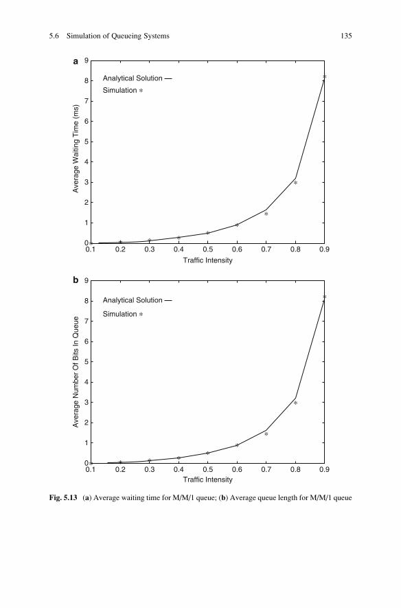
http://dx.doi.org/10.1007/978-3-319-01646-7_4

9a

b

8

7

6

5

Ave

rage

Wai

ting

Tim

e (m

s)

4

3

2

1

00.1 0.2 0.3

Analytical Solution

Simulation

0.4 0.5

Traffic Intensity

0.6 0.7 0.8 0.9

9

8

7

6

5

Ave

rage

Num

ber

Of B

its In

Que

ue

4

3

2

1

00.1 0.2 0.3

Analytical Solution

Simulation

0.4 0.5Traffic Intensity

0.6 0.7 0.8 0.9

Fig. 5.13 (a) Average waiting time for M/M/1 queue; (b) Average queue length for M/M/1 queue


with CST ¼ SERT. The analytical formulas for an M/D/1 queue are found in

Chap. 4, namely:

E Wð Þ ¼ ρ

2μ 1� ρð Þ (5.17)

E Nq

� � ¼ ρ2

2 1� ρð Þ (5.18)

Figure 5.14 show the results for M/D/1 queue. We notice that both the

average waiting time and queue length are half of their respective values for

M/M/1 queue which is confirmed by simulation.

Example 5.3 Develop a computer program to simulate an M/M/n queue assuming

that the arrival rate has a mean value of 1,000 bps and that traffic intensity ρ ¼ 0.1,

0.2, . . .. Calculate and plot the average waiting time and the average queue length in

the queue for n ¼ 2 and n ¼ 5 servers. Compare the results with those of M/M/1

queue.

Solution

We use the flowcharts in Fig. 5.12 to modify the program of the last example.

Since n servers are serving the customers, the value of ρ can be up to n, without

the queue being congested by high number of customer waiting. The analytical

formulas for the average waiting time E(W) and queue length E(Nq) respectively

are given by:

E Wð Þ ¼ ρn ρ=nð Þn! 1� ρ=nð Þ2 p0 (5.19)

E Nq

� � ¼ λE Wð Þ (5.20)

where n is the number of servers and

p0 ¼Xn�1k¼0

ρk

k!þ ρn

n!

1

1� ρ=nð Þ

" #�1(5.21)

The average waiting time and the queue length are given in Fig. 5.15a, b.

We observe good agreement between analytical and simulation results. We can

also see that for a particular value of ρ, both the waiting time and queue length are

smaller for the larger number of servers.

136 5 Simulation

http://dx.doi.org/10.1007/978-3-319-01646-7_4

4.5a

4

3.5

3

2.5

Ave

rage

Wai

ting

Tim

e (m

s)

2

1.5

1

0.5

00.1 0.2 0.3

Analytical Solution

Simulation

0.4 0.5Traffic Intensity

0.6 0.7 0.8 0.9

4.5b

4

3.5

3

2.5

Ave

rage

Num

ber

Of B

its In

Que

ue

2

1.5

1

0.5

00.1 0.2 0.3

Analytical Solution

Simulation

0.4 0.5

Traffic Intensity

0.6 0.7 0.8 0.9

Fig. 5.14 (a) Average waiting time for M/D/1 queue; (b) Average queue length for M/D/1 queue


Fig. 5.15 (a) Average waiting time for M/M/n queue, n ¼ 1, 2, 5. (b) Average queue length for

M/M/n queue, n ¼ 1, 2, 5

138 5 Simulation

5.7 Estimation of Errors

Simulation procedures give solutions which are averages over a number of tests.

For this reason, it is important to realize that the sample statistics obtained from

simulation experiments will vary from one experiment to another. In fact, the

sample statistics themselves are random variables and, as such, have associated

probability distributions, means, variances, and standard deviation. Thus the

simulation results contain fluctuations about a mean value and it is impossible

to ascribe a 100 % confidence in the results. To evaluate the statistical uncer-

tainty or error in a simulation experiment, we must resort to various statistical

techniques associated with random variables and utilize the central limit

theorem.

Suppose that X is a random variable. You recall that we define the expected or

mean value of X as

μ ¼ð1�1

xf xð Þdx (5.22)

where f(x) is the probability density distribution of X. If we draw random and

independent samples, x1, x2, � � �, xN from f(x), our estimate of x would take the

form of the mean of N samples, namely,

eμ ¼ 1

N

XNn¼1

xn (5.23)

Whereas μ is the true mean value of X, eμ is the unbiased estimator of μ—an

unbiased estimator being one with the correct expectation value. Although expected

value eμ is close to μ but eμ 6¼ μ. The standard deviation, defined as

σ xð Þ ¼ E X2� �� μ2

� �1=2(5.24)

provides a measure of the spread in the values of eμ about μ; it yields the order of

magnitude of the error. The confidencewe place in the estimate of themean is given by

the variance of eμ . The relationship between the variance of eμ and the variance of x is

σ eμð Þ ¼ σ xð ÞffiffiffiffiNp (5.25)

This shows that if we use eμ constructed from N values of xn according to

Eq. (5.23) to estimate μ, then the spread in our results ofeμ about μ is proportional toσ(x) and falls off as the number of N of samples increases.

In order to estimate the spread in eμ we define the sample variance

5.7 Estimation of Errors 139

S2 ¼ 1

N � 1

XNn¼1

xn � exð Þ2 (5.26)

Again, it can be shown that the expected value of S2 is equal to σ2(x). Thereforethe sample variance is an unbiased estimator of σ2(x). Multiplying out the square

term in Eq. (5.26), it is readily shown that the sample standard deviation is

S ¼ N

N � 1

1=21

N

XNn¼1

x2n � ex 2

" #1=2(5.27)

For large N, the factor N/(N � 1) is set equal to one.

According to the central limit theorem, the sum of a large number of random

variables tends to be normally distributed, i.e.

f eμð Þ ¼ffiffiffiffiffiN

2π

r1

σ xð Þ exp �N eμ � μð Þ22σ2 xð Þ

" #(5.28)

The normal (or Gaussian) distribution is very useful in various problems in

engineering, physics, and statistics. The remarkable versatility of the Gaussian

model stems from the central limit theorem. For this reason, the Gaussian model

often applies to situations in which the quantity of interest results from the summa-

tion of many irregular and fluctuating components.

Since the number of samples N is finite, absolute certainty in simulation is

unattainable. We try to estimate some limit or interval around μ such that we can

predict with some confidence that eμ falls within that limit. Suppose we want the

probability that eμ lies between μ � ε and μ + ε. By definition,

Prob μ� ε < eμ < μþ ε½ ¼ðμþε

μ�εf eμð Þdeμ (5.29)

By letting λ ¼ eμ�μð Þffiffiffiffiffiffi2=Np

σ xð Þ, we get

Prob μ� ε < eμ < μþ ε½ ¼ 2ffiffiffiπp

ðffiffiffiffiffiffiN=2p� �

ε=σð Þ

0

e�λ2

dλ ¼ erfffiffiffiffiffiffiffiffiffiN=2

p ε

σ xð Þ

(5.30)

or

Prob μ� zα=2σffiffiffiffiNp < eμ < μþ zα=2

σffiffiffiffiNp

� �¼ 1� α (5.31)

where erf(x) is the error function and zα/2 is the upper α/2 � 100 percentile of the

standard normal deviation. The random intervalex � ε is called a confidence interval

140 5 Simulation

and erfffiffiffiffiffiffiffiffiffiN=2

pε=σ xð Þ

� �is the confidence level. Most simulation experiments use

error ε ¼ σ xð Þ= ffiffiffiffiNp

which implies that eμ is within one standard deviation of μ, thetrue mean. From Eq. (5.31), the probability that the sample mean eμ lies within the

interval eμ � σ xð Þ= ffiffiffiffiNp

is 0.6826 or 68.3 %. If higher confidence levels are desired,

two or three standard deviations may be used. For example,

Prob μ�MσffiffiffiffiNp < eμ < μþM

σffiffiffiffiNp

� �¼

0:6826, M ¼ 1

0:954, M ¼ 2

0:997 M ¼ 3

8<: (5.32)

where M is the number of standard deviations. In Eqs. (5.31) and (5.32), it is

assumed that the population standard deviation σ is known. Since this is rarely the

case, σ must be estimated by the sample standard S calculated from Eq. (5.27) so

that the normal distribution is replaced by Student’s t-distribution. It is well known

that the t-distribution approaches the normal distribution as N becomes large, say

N > 30. Thus Eq. (5.31) is equivalent to

Prob μ� Stα=2;N�1ffiffiffiffiNp < eμ < μþ zα=2

Stα=2;N�1ffiffiffiffiNp

� �¼ 1� α (5.33)

where tα/2;N � 1 is the upper 100 � α/2 percentage point of Student’s t-distribution

with (N � 1) degrees of freedom. Its values are listed in any standard statistics text.

The confidence interval ex � ε < x < ex þ ε contains the “true” value of the

parameter x being estimated with a prespecified probability 1 � α. Therefore, whenwe make an estimate, we must decide in advance that we would like to be, say,

90 or 95 % confident of the estimate. The confidence of interval helps us to know

the degree of confidence we have in the estimate. The upper and lower limits of the

confidence interval (known as confidence limits) are given by

upper limit ¼ μþ ε (5.34a)

lower limit ¼ μ� ε (5.34b)

where

ε ¼ Stα=2;N�1ffiffiffiffiNp (5.35)

Thus, if a simulation is performed N times by using different seed values, then in

(1 � α) cases, the estimate eμ lies within the confidence interval and in α cases the

estimate lies outside the interval, as illustrated in Fig. 5.16. Equation (5.35) provides

the error estimate for a given number N of simulation experiments or observations.

If, on the other hand, an accuracy criterion ε is prescribed and we want to

estimate μ by eμ within tolerance of ε with at least probability 1 � α, we must

ensure that the sample size N satisfies

5.7 Estimation of Errors 141

Prob eμ � μ� < ε � 1� α (5.36)

To satisfy this requirement, N must be selected as the small integer satisfying

N � Stα=2;N�1ffiffiffiεp

2

(5.37)

For further discussion on error estimates in simulation, one should consult [17, 18].

Example 5.4 In a simulation experiment, an analyst obtained the mean values of a

certain parameter as 7.60, 6.60, 7.50, and 7.43 for five simulations runs using

different seed values. Calculate the error estimate using a 95 % confidence interval.

Solution

We first get the sample mean

μ ¼ 7:60þ 6:60þ 6:97þ 7:50þ 7:43

5¼ 7:22

From Eq. (5.26), the sample variance is obtained as

S2 ¼ 7:60� 7:22ð Þ2 þ � � � þ 7:43� 7:22ð Þ24

¼ 0:23793

or S ¼ 0.48778. Using a 95 % confidence interval, 1 � α ¼ 95 % (i.e., α ¼ 0.05).

For five runs (N ¼ 5), the t-distribution table gives tα/2;N � 1 ¼ 2.776. Using

Eq. (5.35), the error is estimated as

ε ¼ 0:48778x2:776ffiffiffi5p ¼ 0:6056

Thus, the 95 % confidence interval for the parameter is

μ� ε < eμ < μþ ε ¼ 6:6144 < eμ < 7:78265

μ ε+

μ

μ ε−

•

•

•

•

•

•

•

•

•

•

••

•• •

••

Fig. 5.16 Confidence

of interval

142 5 Simulation

5.8 Simulation Languages

The purpose of this section is to present the characteristics of common simulation

languages and provide the analyst with the criteria for choosing a suitable language.

Once the analyst has acquired a throughout understanding of the system to be

simulated and is able to describe precisely how the model would operate, the next

step is to decide on the language to use in the simulation. This step should not be

taken lightly since the choice of a language would have several implications, some

of which will be discussed later. After deciding on the language to apply, the analyst

needs to consult the language reference manual for all the details.

There are basically two types of languages used in simulation: multipurpose

languages and special-purpose languages. The former are compiler languageswhile the latter are interpretive languages [19]. A compiler language comprises

of macrostatements and requires compilation and assembly before execution can

occur. An interpretive language consists of symbols which denote commands to

carry out operations directly without the need for compilation and assembly. Thus

the major difference between the two types of languages is the distinction between a

source program and an object program. An analyst usually submits a source

program to a computer. If the source program is in a compiler language, an object

program is needed for execution. If the source program is in interpretive language,

execution is done directly without any object program.

Some analysts tend to select multipurpose or general-purpose languages such as

FORTRAN, BASIC, PASCAL, and C for the simulation of computer networks.

Although these languages are far from ideal for discrete simulation, they are widely

been used. Why? There are at least three reasons. First, there is conservatism on the

part of the analysts and organizations that support them. Many organizations are

committed to multipurpose languages and do not want to be vulnerable to a

situation where a code written in a language only familiar to an analyst may have

to be rewritten when the analyst leaves the organization. Second, the widespread

availability of multipurpose languages and the libraries of routines that have been

developed over the years makes them more desirable. It is easy to gain technical

support since experts of multipurpose languages are everywhere. Third, high speed

in the simulation is possible if a general-purpose language is used. Analysts who

prefer fast-running simulations use a general-purpose language. In view of the

problem of learning another set of syntactic rules, a decision in favor of a

general-purpose language is often considered wise by analysts.

The development of special-purpose simulation languages began in the late

1950s. The need came from the fact that many simulation projects required similar

functions across various applications. The purpose of simulation languages is to

provide the analyst with a relatively simple means of modeling systems. Unlike

using the general-purpose language such as C++ where the analyst is responsible

for all the details in the model, special-purpose languages are meant to eliminate the

major portion of the programming effort by providing a simulation-oriented frame-

work about which a model is constructed in a simple fashion. Although many such

languages have been developed, only few have gained wide acceptance.

5.8 Simulation Languages 143

Before deciding which type of language to use in a simulation, the analyst

must carefully weigh the advantages of the multipurpose languages against the almost

guaranteed longer program development and debugging time required in special-

purpose languages. Irrespective of the language used in the simulation of

a computer network, the languagemust be capable of performing functions including:

• generating random numbers,

• executing events,

• managing queues,

• collecting and analyzing data, and

Commonly used special-purpose, discrete simulation languages include GPSS,

SIMSCRIPT, GASP, SLAM, RESQ, NS2, and OPNET. No attempt will be made to

include the many instructions available in these languages. Interested readers must

consult the manuals and references for more details on the languages [20–28].

Only OPNET and NS2 will be covered.

The development of new simulation languages has slowed considerably in the

last few years, and the well established languages have not changed dramatically

for the past few years. This notwithstanding, it is expected that new languages

will be developed and old ones will be improved. At present, there is a growing

interest in combined discrete-continuous simulations. Also, the use of ADA and C

as simulation languages is receiving active attention [32].

5.9 OPNET

Optimized Network Engineering Tools (OPNET) is a window-based comprehen-

sive engineering system that allows you to simulate large communication networks

with detailed protocol modeling. It allows you to design and study communication

networks, devices, protocols, and applications with great flexibility. OPNET key

features include graphical specification of models, a dynamic, event-scheduled

simulation kernel, integrated data analysis tools, and hierarchical, object-based

modeling. Modeler’s object-oriented modeling approach and graphical editors

mirror the structure of actual networks and network components. Modeler supports

all network types and technologies [29].

Here, we focus on the modeling using OPNET IT Guru which is user-friendly

interface with drag-and-drop features that enable users to effectively model, man-

age, and troubleshoot real-world network infrastructures. For example, we illustrate

here how OPNET is used to examine the Medium Access Control (MAC) sublayer

of the IEEE 802.11 standard for wireless local area network (WLAN). The perfor-

mance of different options is analyzed under different scenarios [30].

The model’s concept is overviewed as following: The IEEE 802.11 standard

provides wireless connectivity to computerized stations that require rapid deployment

such as portable computers. The Medium Access Control (MAC) sublayer in the

standard includes two fundamental access methods: distributed coordination function

144 5 Simulation

(DCF) and the point coordination function (PCF). DCF utilizes the carrier sense

multiple access with collision avoidance (CSMA/CA) approach; it is implemented

in all stations in the wireless local area network (WLAN). PCF is based on polling to

determine the station that can transmit next. Stations in an infrastructure network

optionally implement the PCF access method. In addition to the physical CSMA/CD,

DCF and PCF utilize virtual carrier-sense mechanism to determine the state of the

medium. This virtual mechanism is implemented by means of the network allocation

vector (NAV). TheNAVprovides each stationwith a prediction of future traffic on the

medium. Each station uses NAV as an indicator of time periods during which

transmission will not be installed even if the station senses that the wireless medium

is not busy. NAV gets the information about future traffic from management frames

and the header of regular frames being exchanged in the network.

With DCF, every station senses the medium before transmitting. The transmit-

ting station defers as long as the medium is busy. After deferral and while the

medium is idle, the transmitting station has to wait for a random backoff interval.

After the backoff interval and if the medium is still idle, the station initiates data

transmission or optionally exchanges RTS (request to send) and CTS (clear to send)

frames with the receiving station. With PCF, the access point (AP) in the network

acts as a point coordinator (PC). The PC uses polling to determine which station can

initiate data transmission. It is optional for the stations in the network to participate

in PCF and hence respond to poll received from the PC. Such stations are called

CF-pollable stations. The PCF requires control to be gained of the medium by the

PC. To gain such control, the PC utilizes the Beacon management frames to set the

network allocation vector (NAV) in the network stations. As the mechanism used to

set NAV is based on the DCF, all stations comply with the PC request to set their

NAV whether or not they are CF-pollable. This way the PC can control frame

transmissions in the network by generating contention free periods (CFP). The PC

and the CF_pollable stations do not use RTSCTS in the CFP.

The standard allows for fragmentation of the MAC data units into smaller

frames. Fragmentation is favorable in case the wireless channel is not reliable

enough to transmit longer frames. Only frames with a length greater than a

fragmentation and will be separately acknowledged. During a contention period,

all fragments of a single frame will be sent as burst with a single invocation of the

DCF medium access procedure. In case of PCF and during a contention free period,

fragments are sent individually following the rules of the point coordinator (PC),

which will based on the following steps:

5.9.1 Create a New Project

To create a new project for the Ethernet network:

1. Start OPNET IT Guru Academic Edition ! Choose New from the File menu.

2. Select Project ! Click ok ! Name the project < your initials >_WirelessLAN and the scenario DCF ! Click ok

5.9 OPNET 145

3. In the Startup Wizard Initial Topology dialog box, make sure that Create EmptyScenario is selected ! click next ! choose Office from the Network Scale listand check Use Metric Units ! Click next twice ! click ok.

5.9.2 Create and Configure the Network

To create the wireless network:

1. The Object Palette dialog box should be now on the top of your project

workspace.

2. Add to project workspace the following objects from the palette: 9wlan_station_adv (fix).

To add an object from a palette, click its icon in the object palette ! move the

mouse to the workspace ! left-click to place the object. Right-click when

finished.

3. Close the Object Palette dialog box ! Arrange the stations in the workspace as

shown in Fig. 5.17! Save your project.

Fig. 5.17 Workspace to

create and configure the

network

146 5 Simulation

5.9.2.1 Configure the Wireless Nodes

Repeat the following for each of the nine nodes in Fig. 5.17:

1. Right-click on the node ! Edit Attributes ! Assign to theWireless LAN MACAddress attribute a value equal to the node number. Assign to the DestinationAddress attribute the corresponding value shown in Table 5.2! Click ok.

Figure 5.18 shows the values assigned to the Destination Address and WirelessLAN MAC Address attributes for node_1.

5.9.2.2 Traffic Generation Parameters

1. Select all the nodes in the network simultaneously except node_0 ! Right-click

on any of the selected nodes (i.e. node_1 to node_8) ! Edit Attributes !Check the Apply Changes to Selected Objects check box.

Table 5.2 Assignment

of destination address

to the node name

Node name Destination address

Node_1 5

Node_2 8

Node_3 6

Node_4 7

Node_5 1

Node_6 3

Node_7 4

Node_8 2

Fig. 5.18 Values assigned

to the Destination Address

and Wireless LAN MAC

Address attributes for node1

5.9 OPNET 147

2. Expand the hierarchies of the Traffic Generation Parameters and the PacketGeneration Arguments attributes ! Edit the attributes to match the values

shown in Fig. 5.19! Click ok.

3. Select all the nodes in the network simultaneously including node_0 ! Right-

click on any of the selected nodes ! Edit Attributes ! Check the ApplyChanged to Selected Objects check box.

4. Expand the hierarchy of the Wireless LAN Parameters attribute ! Assign the

value 4608000 to the Buffer Size (bits) attribute, as shown in Fig. 5.20! Click

ok.

5. Right-click on node_0 ! Edit Attributes ! Expand the Wireless LANParameters hierarchy and set the Access Point Functionality to Enabled, asshown in Fig. 5.21! Click ok.

5.9.3 Select the Statistics

To test the performance of the network in our DCF scenario, we collect some of the

available statistics as follows:

1. Right-click anywhere in the project workspace and select Choose IndividualStatistics from the pop-up menu.

2. In the Choose Results dialog box, expand the Global Statistics and NodeStatistics hierarchies ! choose the five statistics, as shown in Fig. 5.22.

3. Click ok and then save your project.

Fig. 5.19 Traffic

generation parameters

for node 1

148 5 Simulation

5.9.4 Configure the Simulation

Here we will configure the simulation parameters:

1. Click on the Configure Simulation button.

2. Set the duration to be 10.0 min.

3. Click ok and then save your project.

Fig. 5.20 Editing

buffer size

Fig. 5.21 Enabled the

access point functionality

for node 0

5.9 OPNET 149

5.9.5 Duplicate the Scenario

In the network we just created, we did not utilize many of the features explained in

the overview. However, by default the distributed coordination function (DCF)

method is used for the medium access control (MAC) sublayer. We will create three

more scenarios to utilize the features available from the IEEE 802.11 standard. In

the DCF_Frag scenario we will allow fragmentation of the MAC data units into

smaller frames and test its effect on the network performance. The DCF_PCF

scenario utilizes the point coordination function (PCF) method for the medium

access control (MAC) sublayer along with the DCF method. Finally, in the

DCF_PCF_Frag scenario we will allow fragmentation of the MAC data and

check its effect along with PCF.

5.9.5.1 The DCF_Frag Scenario

1. Select Duplicate Scenario from the Scenarios menu and give it the name

DCF_Frag ! click ok.

Fig. 5.22 The Chosen statistics results we want to show up

150 5 Simulation

2. Select all the nodes in the DCF_Frag scenario simultaneously ! Right-click

on anyone of them ! Edit Attributes ! Check the Apply Changes to SelectedObjects check box.

3. Expand the hierarchy of the Wireless LAN Parameters attribute ! Assign the

value 256 to the Fragmentation Threshold (bytes) attribute, as shown in

Fig. 5.23! Click ok.

4. Right-click on node_0 ! Edit Attributes ! Expand the Wireless LANParameters hierarchy and set the Access Point Functionality to Enabled as

shown in Fig. 5.24! Click ok.

Fig. 5.23 DCF_Frag Scenario for node 8

Fig. 5.24 Enabled the access point functionality for node 0

5.9 OPNET 151

5.9.5.2 The DCF_PCF Scenario

1. Switch to the DCF scenario, select Duplicate Scenario from the Scenariosmenu

and give it the name DCF_PCF ! Click ok ! Save your project.

2. Select node_0, node_1, node_3, node_5 and node_7 in the DCF_PCF scenario

simultaneously ! Right-click on anyone of the selected nodes ! EditAttributes.

3. Check Apply Changes to Selected Objects ! Expand the hierarchy of the

Wireless LAN Parameters attribute ! Expand the hierarchy of the PCFParameters attribute ! Enable the PCF Functionality attribute, as shown in

Fig. 5.25! Click ok.

4. Right-click on node_0 ! Edit Attributes ! Expand the Wireless LANParameters hierarchy and set the Access Point Functionality to Enabled, asshown in Fig. 5.26.

5. Click ok and save your project.

5.9.6 Run the Simulation

To run the simulation for the four scenarios simultaneously.

1. Go to the Scenarios menu ! Select Manage Scenarios.

Fig. 5.25 Enabling PCF

Parameters for node 0

152 5 Simulation

2. Click on the row of each scenario and click the Collect Results button. This

should change the values under the Results column to < collect > shown in

Fig. 5.27.

3. Click ok to run the four simulations.

4. After the simulation of the four scenarios complete, click Close and then save

your project.

5.9.7 View the Results

To view and analyze the results:

1. Select Compare Results from the Results menu.

Fig. 5.27 Managing the Scenarios

Fig. 5.26 Enabled the access point functionality for node 0

5.9 OPNET 153

2. Change the drop-down menu in the lower right part of the Compare Resultsdialog box from As Is to time-average ! Select the Delay (sec) statistic from

the Wireless LAN hierarchy as shown in Fig. 5.28.

3. Click Show to show the result in a new panel. The resulting graph should

resemble that shown in Fig. 5.29.

Fig. 5.28 Comparing results

Fig. 5.29 Time average in WLAN delay (s)

154 5 Simulation

4. Go to the Compare Results dialog ! Follow the same procedure to show the

graphs of the following statistics from theWireless LAN hierarchy: Load (bits/s)and Throughput (bits/s). The resulting graphs should resemble Figs. 5.30

and 5.31.

Fig. 5.30 Time average

in WLAN load (bits/s)

Fig. 5.31 Time average in

WLAN throughput (bits/s)

5.9 OPNET 155

5. Go to the Compare Results dialog box ! Expand the Object Statistics hierarchy! Expand the Office Network hierarchy ! Expand the hierarchy of two nodes.

One node should have PCF enabled in the DCF_PCF scenario (e.g., node_3) and

the other node should have PCF disabled (e.g., node_2) ! Show the result of

the Delay (sec) statistic for the chosen nodes. The resulting graphs should

resemble Figs. 5.32 and 5.33.

6. Repeat step 5 above but for the Retransmission Attempts (packets) statistic. Theresulting graphs should resemble Figs. 5.34 and 5.35.

7. Close all graphs and the Compare Results dialog box ! Save your project.

More information about Opnet can be found in [31].

5.10 NS2

The Network Simulator version 2 (NS2) is targeted at networking. It is

object-oriented, discrete event driven network simulator. It was developed at UC

Berkeley written in C++ language and it uses Object-oriented extension of Tool

command language (OTcl). These two different languages are used for different

purposes in NS2 as shown in Table 5.3 and more information about NS2 can be

found in [32, 33].


WLAN delay (s) for node 3

156 5 Simulation

Figure 5.36 shows the process of network simulation in NS2. The simulation

using NS2 can carry two levels: first level is based on configuration and con-

struction of OTcl, and second level, is based on OTcl and C++. It is essential for

NS2 to be upgraded or modified to add the required elements when the module

resources needed do not exist. Therefore, the split object model of NS2 is used to


WLAN delay (s) for node 2


WLAN retransmission line

attempts (packets) for

node 3

5.10 NS2 157

add a new C++ class and an OTcl class, and then program the OTcl scripts to

implement the simulation [34]. The class hierarchies of C++ and OTcl languages

can be either stand alone or linked together using an OTcl/C++ interface called

TclCL [32].

There are three components for whole network simulation using NS2 [35]. First,

modifying the source code. This step is used only when there is a need to modify the

source codes which requires programming and debugging from the users. Indeed,

the OTcl codes need to be modified as the source codes due to that NS2 supports the

OTcl and C++. Second, writing the Tcl/OTcl scripts of network simulations. In fact,


WLAN retransmission line

attempts (packets) for

node 2

Table 5.3 Use of OTcl and C++

OTcl C++

Acts as the front end (i.e., user interference,

a command and configuration)

Acts as the back end running the actual

simulation

NS2 uses it to create and configure a network NS2 uses it to run simulation

OTcl is an interpreter All C++ codes need to be complied and linked

to create an executable file

Use OTcl for configuration, setup, and one

time simulation

Use C++ for dealing with a packet

Use OTcl for run simulation with existing

NS2 models

Use C++ for the need to modify existing

NS2 modules

OTcl is slow to run, but fast to change,

therefore, it is suitable to run a small

simulation configuration over several

repetitions.

C++ is fast to run and slow to change, therefore,

it is suitable for the detailed protocol

implementation procedures and large

simulation

158 5 Simulation

in this step, it requires the user writing Tcl codes for describing the network

topology types, defining nodes and network component attributes, controlling the

network simulation process. Third, analyzing the network simulation results.

This step requires the user to understand the structure of the NS2 Trace file and

to be able to use some tools to check the outcome data and draw figures, etc.

Figure 5.37 shows the flow chart for simulation in NS2. Although, the general

architecture of the view of the NS2 for the general users can be presented in

Fig. 5.38.

NS2 is primarily useful for simulating LAN and WAN. It has the capability of

supporting the simulations of unicast node and multicast node. It is complemented

by Network Animator (NAM) for packet visualization purposes such as Fig. 5.39

for simulation topology of wireless network [37]. Indeed, NS2 is widely used

network simulator that has been commonly used in education and research.

NS2 has the following limitations [36]:

1. Large multi format outcome files, which require post processing.

2. Huge memory space consumption due to a very large output file.

3. Relatively slow.

4. Lack of built-in-QoS monitoring modules.

5. Lack of user friendly visual output representation.

6. Requires the users to develop tools by themselves.

Fig. 5.36 The simulation process of NS2 [34]

5.10 NS2 159

5.11 Criteria for Language Selection

There are two types of factors that influence the selection of the special-purpose

language an analyst uses in his simulation. One set of factors is concerned with the

operational characteristics of the language, while the other set is related to its

problem-oriented characteristics [38, 39].

In view of the operational characteristics of a language, an analyst must consider

factors such as the following:

Fig. 5.37 The simulation flow chart of NS2 [35]

160 5 Simulation

1. the analyst’s familiarity with the language;

2. the ease with which the language can be learned and used if the analyst is not

familiar with it;

3. the languages supported at the installation where the simulation is to be done;

4. the complexity of the model;

5. the need for a comprehensive analysis and display of simulation results;

6. the language’s provision of good error diagnostics;

Fig. 5.38 The architectural view of NS2 [36]

Fig. 5.39 Network animator interface (NAM) showing the simulation topology of wireless

network [37]

5.11 Criteria for Language Selection 161

7. the compiling and running time efficiency of the language;

8. the availability of well written user’s manual;

9. the availability of support by a major interest group; and

10. the cost of installation, maintenance, and updating of the language.

In the view of the characteristics of the language and those of the problems the

analyst will most likely encounter, the following factors should be considered:

1. time advance methods;

2. random number and random variate generation capabilities;

3. the way a language permits the analyst to control the sequence of subroutines

that represent the state changes;

4. capability for inserting use-written subroutines; and

5. forms of statistical analyses that can be performed on the data collected during

simulation.

No language is without some strong points as well as weak points. It is difficult

to compare these languages because many important software features are quite

subjective in nature. Everyone seems to have his own opinion concerning the

desirable features of a simulation language, e.g. ease of model development,

availability of technical assistance, and system compatibility. In spite of this

difficulty, various attempts have been made to compare simulation languages

based on objective criteria [22]. In general, GPSS and SLAM (which are

FORTRAN-based) are easiest to learn.

SIMSCRIPT has the most general process approach and thus can be used to

model any system without using the event-scheduling approach. This, however,

may result in more lines of code than GPSS or SLAM. RESQ has features specially

oriented toward computer and communication systems, but the terminology is

strictly in terms of queueing networks.

5.12 Summary

1. This chapter has presented the basic concepts and definitions of simulation

modeling of a system.

2. The emphasis of the chapter has been on discrete, stochastic, digital, software

simulation modeling. It is discrete because it proceeds a step at a time. It is

stochastic or nondeterministic because element of randomness is introduced by

using random numbers. It is digital because the computers employed are digital.

It is software because the simulation model is a computer program.

3. Because simulation is a system approach to solving a problem, we have consid-

ered the major stages involved in developing a model of a given system.

These stages are model building.

4. Since simulation output is subject to random error, the simulator would

like to know how close is the point estimate to the mean value μ it is supposed

to estimate. The statistical accuracy of the point estimates is measured in

162 5 Simulation

terms of the confidence interval. The simulator generates some number of

observations, say N, and employs standard statistical method to obtain the

error estimate.

5. There are basically two types of languages used in simulation: multipurpose

languages and special-purpose languages. The multipurpose or general-purpose

languages include FORTRAN, BASIC, ADA, PASCAL, and C++. Special-

purpose languages are meant to eliminate the major portion of the programming

effort by providing a simulation-oriented framework about which a model is

constructed in a simple fashion.

6. A brief introduction to two commonly used special-purpose, discrete simulation

packages (NS2 and OPNET) is presented.

More information about simulation can be found in the references,

including [40].

Problems

5.1 Define simulation and list five attractive reasons for it?

5.2 Generate 10,000 random numbers uniformly distributed between 0 and

1. Find the percentage of numbers between 0 and 0.1, between 0.1 and 0.2,

etc., and compare your results with the expected distribution of 10 % in each

interval.

5.3 (a) Using the linear congruential scheme, generate ten pseudorandom num-

bers with a ¼ 1573, c ¼ 19, m ¼ 1000, and seed value X0 ¼ 89.

(b) Repeat the generation with c ¼ 0.

5.4 Uniformly distributed random integers between 11 and 30, inclusive, are to

be generated from the random numbers U shown below. How many of the

integers are odd numbers?

0.2311 0.7919

0.2312 0.9218

0.6068 0.7382

0.4860 0.1763

0.8913 0.4057

0.7621 0.9355

0.4565 0.9169

0.0185 0.4103

0.8214 0.8936

0.4447 0.0579

5.5 Generate 500 random numbers, exponentially distributed with mean 4,

using uniformly distributed random numbers U. Estimate the mean and the

variance of the variate.

Problems 163

5.6 Using the rejection method, generate a random variable from

f xð Þ ¼ 5x2, 0 � x � 1

5.7 (a) Using the idea presented in this chapter, generate 100 Gaussian variates

with mean 3 and variance 2.

(b) Repeat part (a) using MATLAB command randn.

(c) By estimating the mean and variance, which procedure is more accurate?

5.8 The probability density function of Erlang distribution is

f xð Þ ¼ αkxk�1

Γ kð Þ e�αx, x > 0, α > 0

where Γ(k) ¼ (k � 1)! and k is an integer. Take k ¼ 2 and α ¼ 1. Use the

rejection method to describe a procedure for generating random variates from

Erlang distribution.

5.9 Write a computer program to produce variates that follow hyperexponential

distribution, i.e.

f xð Þ ¼ pλe�λx þ 1� pð Þμe�μx

Take p ¼ 0.6, λ ¼ 10, μ ¼ 5.

5.10 Write a program to simulate the M/Ek/1 queueing system. Take k ¼ 2.

Compare the results of the simulation with those predicted by queueing

theory.

5.11 A random sample of 50 variables taken from a normal population has a mean

of 20 and standard deviation of 8. Calculate the error with 95 % confidence

limits.

5.12 In a simulation model of a queueing system, an analyst obtained the mean

waiting time for four simulation runs as 42.80, 41.60, 42.48, and 41.80 μs.Calculate the 98 % confidence interval for the waiting time.

5.13 Discuss the OPNET simulation results of Fig. 5.29 results?

5.14 Discuss the OPNET simulation comparison results of Figs. 5.30 and 5.31?

5.15 Discuss the OPNET simulation comparison results Figs. 5.32 through 5.35?

5.16 What are different purposes for C++ and OTcl languages in NS2?

5.17 What are the limitations of NS2?

References

1. S. V. Hoover and R. F. Perry, A Problem Solving Approach. New York: Addison-Wesley,

1989.

2. F. Neelamkavil, Computer Simulation and Modelling. Chichester: John Wiley & Sons, 1987,

pp. 1-4.

164 5 Simulation

3. M. H. MacDougall, Simulating Computer Systems: Techniques and Tools. Cambridge, MA:

MIT Press, 1987, p. 1.

4. J. W. Schmidt and R. E. Taylor, Simulation and Analysis of Industrial Systems. Homewood,

IL: R. D. Irwin, 1970, p. 5.

5. J. Banks and J. S. Carson, Discrete-event System Simulation. Englewood Cliffs, NJ: Prentice-

Hall, 1984, pp. 3-16.

6. W. Delaney and E. Vaccari, Dynamic Models and Discrete Event Simulation. New York,

Marcel Dekker, 1989, pp. 1,13.

7. G. S. Fishman, Concepts and Methods in Discrete Event Digital Simulation. New York: John

Wiley & Sons, 1973, pp. 24-25.

8. W. J. Graybeal and U. W. Pooch, Simulation: Principles and Methods. Cambridge, MA:

Winthrop Publishers, 1980, pp. 5-10.

9. T. G. Lewis and B. J. Smith, Computer Principles of Modeling and Simulation. Boston, MA:

Houghton Mifflin, 1979, pp. 172-174.

10. M. N. O. Sadiku and M. Ilyas, Simulation of Local Area Networks. Boca Raton: CRC Press,

1995, pp. 44,45, 67-77.

11. A. M. Law and W. D. Kelton, Simulation of Modeling and Analysis. New York: McGraw-Hill,

2nd ed., 1991, pp. 420-457.

12. R. McHaney, Computer Simulation: a Practical Perspective. New York: Academic Press,

1991, pp. 91-95, 155-172.

13. H. Kobayashi, Modeling and Analysis: An Introduction to System Performance EvaluationMethodology. Reading, MA: Addison-Wesley, 1978

14. R. Jain, The Art of Computer Systems Performance Analysis. New York: John Wiley & Sons,

1991, pp. 474-501.

15. M.N.O. Sadiku and M. R. Tofighi, “A Tutorial on Simulation of Queueing Models,” Interna-tional Journal of Electrical Engineering Education, vol. 36, 1999, pp. 102-120.

16. M. D. Fraser, “Simulation,” IEEE Potential, Feb. 1992, pp. 15-18.17. M. H. Merel and F. J. Mullin, “Analytic Monte Carlo error analysis,” J. Spacecraft, vol. 5, no.

11, Nov. 1968, pp. 1304 -1308.

18. A. J. Chorin, “Hermite expansions in Monte-Carlo computation,” J. Comp. Phys., vol. 8, 1971,

pp. 472 -482.

19. G. S. Fishman, Concepts and Methods in Discrete Event Digital Simulation. New York: John

Wiley & Sons, 1973, pp. 92-96.

20. G. Gordon, “A General Purpose Systems Simulation Program,” Proc. EJCC, Washington

D.C. New York: Macmillan, 1961.

21. J. Banks, J. S. Carson, and J. N. Sy, Getting Started with GPSS/H. Annandale, VA: Wolverine

Software, 1989.

22. Minuteman Software: GPSS/PC Manual. Stow: MA, 1988.

23. B. Schmidt, The Simulator GPSS-FORTRAN Version 3. New York: Springer Verlag, 1987.

24. H. M. Markowitz, B. Hausner, and H. W. Karr, SIMSCRIPT: A Simulation ProgrammingLanguage. Englewood Cliffs, NJ: Prentice-Hall, 1963.

25. P. J. Kiviat, R. Villaneuva, and H. M. Markowitz, The SIMSCRIPT II Programming Language.Englewood Cliffs, NJ: Prentice-Hall, 1968.

26. A. A. B. Pritsker, The GASP IV Simulation Language. New York: John Wiley & Sons, 1974.

27. A. A. B. Pritsker, Introduction to Simulation and SLAM II. New York: JohnWiley & Sons, 2nd

ed., 1984.

28. J. F. Kurose et al., “A graphics-oriented modeler’s workstation environment for the RESearch

Queueing Package (RESQ),” Proc. ACM/IEEE Fall Joint Computer Conf., 1986.29. I. Katzela, Modeling and Simulation Communication Networks. Upper Saddle River, NJ:

Prentice Hall, 1999.

30. E. Aboelela, Network Simulation Experiments Manual. London, UK: Morgan Kaufmann,

2008, pp. 173–184.

31. http://www.opnet.com/

References 165

http://www.opnet.com/

32. T. Issarikakul and E. Hossain, “Introduction to Network Simulator NS2. Springer, 2009.

33. http://www.isi.edu/nsnam/ns/

34. L. Fan and L. Taoshen, “Implementation and performance analyses of anycast QoS routing

algorithm based on genetic algorithm in NS2,” Proceedings of Second International Confer-ence on Information and Computing Science, 2009, pp. 368 – 371.

35. S. Xu and Y. Yang, “Protocols simulation and performance analysis in wireless network based

on NS2,” Proceedings of International conference on Multimedia Technology (ICMT), 2011,

pp. 638 – 641.

36. M. J. Rahimi et al., “Development of the smart QoS monitors to enhance the performance of

the NS2 network simulator,” Proceedings of 13th International Conference on computer andInformation Technology, 2010, pp. 137-141.

37. R. Huang et al., “Simulation and analysis of mflood protocol in wireless network,”

Proceedings of International Symposium on Computer Science and Computational Technol-ogy, 2008, pp. 658-662.

38. W. J. Graybeal and U. W. Pooch, Simulation: Principles and Methods. Cambridge, MA:

Winthrop Publishers, 1980, p. 153.

39. J. R. Emshoff and R. L. Sisson, Design and Use of Computer Simulation Models. London:Macmillan, 1970, pp. 119-150.

40. D. Maki and M. Thompson,Mathematical modeling and Computer Simulation. Belmont, CA:

Thomson Brooks/Cole, 2006, pp. 153-211.

166 5 Simulation

http://www.isi.edu/nsnam/ns/

Chapter 6

Local Area Networks

Success doesn’t discriminate. It’s an equal opportunityemployer—available to everyone willing to pay the price.

—Anonymous

When designing a local area network (LAN), establishing performance

characteristics of the network before putting it into use is of paramount importance;

it gives the designer the freedom and flexibility to adjust various parameters of the

network in the planning rather than the operational phase. However, it is hard to

predict the performance of the LAN unless a detailed analysis of a similar network

is available. Information on a similar network is generally hard to come by so that

performance modeling of the LAN must be carried out.

In this chapter we focus on the analytic models of four LAN important protocols:

the token-passing access methods for the ring and bus topologies, the CSMA/CD

for bus, and the star. The analytic models provide an insight into the nature of the

networks. It should be emphasized that for each network, we do not provide all the

details; that can be found in the references. We provide enough detail to understand

the performance analysis, which is our focus.

Before we present the analytic model for each network, it is expedient that we

consider the OSI reference model, which applies to LANs, MANs, and WANs.

6.1 OSI Reference and IEEE Models

An effective solution to communication between diverse equipment by numerous

manufacturers is to have vendors abide by a common set of rules or data-exchange

protocols. In 1973, the International Standards Organization (ISO) issued a recom-

mendation for a standard network architecture. This is known as the Open System


167

Interconnection (OSI) reference model. “Open” refers to the ability to communicate

with any other system obeying the same standards.

The OSI reference model is a structured model. It is divided into seven layers as

shown in Fig. 6.1 and explained as follows.

The application layer, layer 7, is the one the user sees. It provides services

directly comprehensible to application programs; login, password checks, network

transparency for distribution of resources, file and document transfer, industry

specific protocols.

The presentation layer, layer 6, is concerned with the interpretation of the data.

It restructures data to/from standardized format used within network; text compres-

sion, code conversion, file format conversion, and encryption.

The session layer, layer 5, manages address translation and access security. It

negotiates to establish a connection with another node on the network and then to

manage the dialogue. This means controlling the start, stopping, and

synchronisation of the conversion.

The transport layer, layer 4, performs error control, sequence checking,

handling of duplicate packets, flow control, and multiplexing. Here it is determined

whether the channel is to be point-to-point (virtual) with ordered messages, isolated

messages with no order, or broadcast messages. It is the last of the layers which are

concerned with communications between peer entities in the systems. The transport

layer and above are referred to as the upper layers of the model, and they are

independent of the underlying network. The lower layers are concerned with data

transfer across the network.

The network layer, layer 3, provides a connection path between systems, includ-

ing the case where intermediate nodes are involved. It deals with message

packetization, message routing for data transfer between non-adjacent nodes or

stations, congestion control, and accounting.

The data-link layer, layer 2, establishes the transmission protocol, the way in

which information will be transmitted, acknowledgment of message, token posses-

sion, error detection, and sequencing. It prepares the packets passed down from the

network layer for transmission on the network. It takes a raw transmission and

transforms it into a line free from error. Here headers and framing information are

OSI Model IEEE LAN Layers

7

6

5

4

3

2

1

Application

Presentation

Session

Transport

Network

Data Link

Physical

Higher-levelprotocols

Physical

Medium accessLogical Link


between the OSI model

and IEEE LAN layers

168 6 Local Area Networks

added or removed. With these go the timing signals, check-sum, and station

addresses, as well as the control system for access.

The physical layer, layer 1, is that part that actually touches themedia or cable; the

line is the point within the node or device where the data is received and transmitted.

It sees to it that ones arrive as ones and zeros as zeros. It encodes and physically

transfers messages (raw bits stream) between adjacent stations. It handles voltages,

frequencies, direction, pin numbers, modulation techniques, signaling schemes,

ground loop prevention, and collision detection in CSMA/CD access method.

A good way to remember the layers is this. Starting from the layer 1, one should

remember the saying, “Please Do Not Throw Sausage Pizza Away.”

The IEEE has formulated standards for the physical and logical link layers for

three types of LANs, namely, token buses, token rings, and CSMA/CD protocols.

Figure 6.1 illustrates the correspondence between the three layers of the OSI and the

IEEE 802 reference models. The physical layer specifies means for transmitting and

receiving bits across various types of media. The media access control layer

performs the functions needed to control access to the physical medium. The logical

link control layer is the common interface to the higher software layers.

6.2 LAN Characteristics

A local area network (LAN) is distinguished from other types of computer networks

in that communication is usually confined to a moderate geographical area such as a

building or a campus. It has the following characteristics:

• Short distance (up to 1 km)

• High speed (1–100 Mbps)

• Low error rate (10�8 to 10�4)• Ease of access

A LAN is usually owned by a single organization and it is designed for the

purpose of sharing resources.

The topology of a network is the way in which the nodes (or stations) are

interconnected. The basic forms of LAN topologies are shown in Fig. 6.2.

The type of technology used to implement LANs are diverse as the LAN

vendors. Both vendors and users are forced to make a choice. This choice is usually

based on several criteria such as:

– network topology and architecture

– access control

– transmission medium

– transmission techniques (baseband/broadband signaling)

– adherence to standards

– performance in terms of channel utilization, delay, and power

The primary performance criterion is the delay-throughput characteristics

of the system.

6.2 LAN Characteristics 169

Themean transfer delay of a message is the time interval between the instant the message

is available at the sending station and the end of its successful reception at the receiving

station.

It is convenient to regard the transfer delay as comprising of three components.

The first component, W, is called the waiting time or access time. It is the time

elapsed from the availability of a message in the source station transmit buffer until

the beginning of its transmission on the channel. The second component, Tp, called

the propagation time, is the time elapsed from the beginning of the transmission of

the message until the arrival of the first bit of the message at the destination. The

third component is the transmission or service time, S, which is the time elapsed

between the arrival of the first bit of the message at the destination and the last bit.

As soon as the last bit arrives at the destination, the transfer is complete. This

implies that the transfer delay D includes the waiting time W (or queueing delay) at

the sending station, the service (or transmission) time S of the message, and the

propagation delay Tp, i.e.

D ¼Wþ Sþ Tp (6.1a)

In terms of their expected values

E Dð Þ ¼ E Wð Þ þ E Sð Þ þ E�Tp

�(6.1b)

(bus)

(ring)

(star)

(tree)

Fig. 6.2 Typical LAN

topologies


6.3 Token-Passing Ring

The token-passing ring, developed by workers at the Zurich Research Laboratories

of IBM in 1972 and standardized as an access method in the IEEE Standard 802.5,

is the best-known of all the ring systems. Here we are interested in its basic

operation and delay analysis [3–4].

6.3.1 Basic Operation

In a token ring, the stations are connected as in all ring networks as illustrated in

Fig. 6.3.

Access to the transmission channel is controlled by means of a special eight-bit

pattern called a token, which is passed around the ring. When the system is

initialized, a designated station generates a free token, such as 11111111. If no

station is ready to transmit, the free token circulates around the ring. When a station

wishes to transmit, it captures the free token and changes it to a busy token, such as

11111110, thereby disallowing other stations from transmitting. The packet to be

transmitted is appended to the busy token. The receiving station copies the infor-

mation. When the information reaches the sending station, the station takes it off the

ring and generates a new free token to be used by another station who may need the

transmission channel.

This operation can be described by a single-server queueing model, as illustrated

in Fig. 6.4.

The server serves as many queues as stations attached to the ring. The server

attends the queues in a cyclic order as shown by the rotating switch which

Ring interface unit

Fig. 6.3 A typical ring

topology

6.3 Token-Passing Ring 171

represents the free token. Once a station captures the token, it is served according to

one of the following service disciplines:

• Exhaustive service: the server serves a queue until there are no customers left in

that queue.

• Gated service: the server serves only those customers in a queue that were

waiting when it arrived at that queue, i.e. when the server arrives at a queue, a

gate is closed behind the waiting customers and only those customers in front of

the gate are served.

• Limited service: the server serves a limited number of customers, say K (con-

stant) or less, that were waiting when it arrived at the queue.

6.3.1.1 Delay Analysis

Consider a single server serving N queues in a cyclic manner as shown in Fig. 6.4.

Let ri denote a constant switchover time from queue i to queue i+1 and Ro be the

sum of all switchover times, i.e.

r1 r2

r3

H1

r4

λ1 λ2 λ3 λ4Fig. 6.4 Cyclic-service

queueing model


Ro ¼XNi¼1

ri (6.2)

We examine the M/G/1 model, that is, messages arrive at queues according to

independent Poisson processes with mean rates λ1, λ2, � � �, λN and the service times

Hi of the messages from queue i are generally distributed with mean E(Si) and

second moment E(Si2). We denote the utilization of queue i by

ρi ¼ λiE Sið Þ (6.3)

and assume that the normalization condition:

ρ ¼XNi¼1

ρi < 1 (6.4)

Let Vi denote the intervisit time of queue i, also known as the server-vacation

time, the time interval from the server’s departure from the queue until its return to

the same queue. The moment generating function for the statistical-equilibrium

waiting time distribution is given by [5–7]:

Exhaustive service:

GeW zð Þ ¼ E e�zWi

� � ¼ 1� ρiE Við Þ

1� Gv zð Þz� λi þ λiGs zð Þ (6.5)

Gated service:

GgW zð Þ ¼ Gc zð Þλi 1� Gs zð Þ½ � � Gc zð Þ

E Við Þ z� λi þ λiGs zð Þ½ � (6.6)

Limited service:

GlW zð Þ ¼ 1� ρi þ λiE Við Þ

E Við Þ1� Gv zð Þ

z� λi þ λiGs zð ÞGv zð Þ (6.7)

where Gv zð Þ ¼ E e�zVið Þ is the generating function for the intervisit time;

Gs zð Þ ¼ E e�zSið Þ is the generating function for the service time,

Gc zð Þ ¼ E e�zCi� �

is the generating function for the cycle time.

From Eqs. (6.5)–(6.7), the mean waiting time of messages in queue i is deter-

mined by differentiating GW(z) and setting z ¼ 0. The result is:

Exhaustive service:

Ee Wið Þ ¼ E Við Þ2þ Var Við Þ

2E Við Þ þλiE S2i

� �2 1� ρið Þ (6.8)


Gated service:

Eg Wið Þ ¼ E Cið Þ2þ Var Cið Þ

2E Cið Þ þρiE S2i

� �2 1� ρið ÞE Sið Þ (6.9)

Limited service:

El Wið Þ ¼λiE Vi þ Sið Þ2

h i2 1� ρi þ λiE

�Vi

�ih i (6.10)

Hence the mean waiting time can be found provided the first two moments of the

intervisit times Vi are known.

To find the first moment of Vi, let Ci be the total cycle time (i.e. the time between

subsequent visits of the server to queue i) and Ti be the time spent by the server at

queue i, then

E Við Þ ¼ E Cið Þ � E Tið Þ (6.11)

It is readily shown that [8]

E Cið Þ ¼ Ro

1� ρ(6.12)

Since the traffic flow must be conserved, the average number of messages

serviced during one visit of queue i is equal to the average number of arriving

messages at that queue in one cycle time, i.e.

E Tið ÞE Sið Þ ¼ λiE Cið Þ

or

E Tið Þ ¼ λiE Cið ÞE Sið Þ ¼ ρiE Cið Þ (6.13)

Substituting Eqs. (6.12) and (6.13) into Eq. (6.11) gives the mean intervisit time

of queue i as

E Við Þ ¼ 1� ρi1� ρ

Ro (6.14)

Introducing Eqs. (6.12) and (6.14) in Eq. (6.8) leads to

Ee Wið Þ ¼ Var Við Þ2E Við Þ þ

1� ρi2 1� ρð ÞRo þ ρi

2 1� ρið ÞE S2i� �E Sið Þ (6.15)


for exhaustive service. Taking similar procedure for gated service discipline

results in

Eg Wið Þ ¼ Var Við Þ2E Við Þ þ

1þ ρi2 1� ρð ÞRo þ ρi

2 1� ρið ÞE S2i� �E Sið Þ (6.16)

For limited service, we have an explicit solution for E(Wi) only in the special

case of statistically symmetric conditions and K ¼ 1 for all stations [5, 7]. However,

an upper bound for E(Wi) for any K is presented in [9].

For symmetric traffic conditions (i.e. in the case of identical stations),

λ1 ¼ λ2 ¼ � � � ¼ λN ¼ λ

N(6.17)

r1 ¼ r2 ¼ � � � ¼ rN ¼ Ro

N¼ r (6.18)

and the mean waiting time for all the queues becomes:

Exhaustive service:

Ee Wið Þ ¼ δ2

2rþ Nr 1� ρ=Nð Þ

2 1� ρð Þ þ ρE S2� �

2 1� ρð ÞE Sð Þ (6.19)

Gated service:

Eg Wið Þ ¼ δ2

2rþ Nr 1þ ρ=Nð Þ

2 1� ρð Þ þ ρE S2� �

2 1� ρð ÞE Sð Þ (6.20)

Limited service:

Ee Wið Þ ¼ δ2

2rþ Nr 1þ ρ=Nð Þ þ Nλδ2

2 1� ρ� Nλrð Þ þ ρE S2� �

2 1� ρ� Nλrð ÞE Sð Þ (6.21)

where δ2 is the variance of the switchover time. An alternative, less rigorous means

of deriving Eqs. (6.19–6.21) is the decomposition theorem [8]. Note that the only

difference between Eqs. (6.19) and (6.20) is the � signs in the terms (1 � ρ) whichimplies that Ee(W ) � Eg(W ). Thus, from Eqs. (6.19)–(6.21), we conclude that:

Ee Wð Þ � Eg Wð Þ � El Wð Þ (6.22)

The above derivations are for continuous-time systems. The corresponding

derivations for discrete-time systems can be found in [5, 9–11].

The formulas in Eqs. (6.19)–(6.21) for the waiting time are valid for token ring

and token bus. However, the mean value r of the switchover time and its variance

δ2 differ for each protocol. Here we evaluate these parameters for the token ring.


The token passing interval or switchover time T is given by

T ¼ Tt þ Tpt þ Tb (6.23)

where Tt is the token transmission time, Tpt is the token propagation delay, and Tb is

the bit delay per station. Hence, the expected value r ¼ E(T) is given by

r ¼ E Ttð Þ þ E Tpt

� �þ E Tbð Þ (6.24)

and, since the random variables are independent, the variance Var (T) ¼ δ2 is

given by

δ2 ¼ Var Tið Þ þ Var Tpt

� �þ Var Tbð Þ (6.25)

Assuming a constant token packet length Lt (including preamble bits), for a

network data rate R,

Tt ¼ LtR

Its expected value is constant. Hence

E Ttð Þ ¼ Tt ¼ LtR, Var Ttð Þ ¼ 0 (6.26)

Assuming that the stations are equally spaced on the ring, the distance between

any adjacent stations is identical to l=N, where l is the physical length of the ring. IfP is the signal propagation delay in seconds per unit length (the reciprocal of the

signal propagation delay velocity u, i.e. P ¼ 1/u), the token propagation delay is

Tpt ¼ Pl

N

Hence

E Tpt

� � ¼ Tpt ¼ Pl

N, Var Tpt

� � ¼ 0 (6.27)

If Lb is the bit delay caused by each station,

Tb ¼ LbR

and

E Tbð Þ ¼ LbR, Var Tbð Þ ¼ 0 (6.28)


We conclude from Eqs. (6.24)–(6.28) that

r ¼ Pl

Nþ Lb þ Lt

R, δ2 ¼ 0 (6.29)

The average propagation delay suffered from one station is the propagation

delay halfway around the ring, i.e.

E Tp

� � ¼ τ=2 (6.30)

where τ is the round-trip propagation delay. Note that the sum of the switchover

times (assumed to be constant) corresponds to the round-trip propagation delay and

the sum of the bit-holding times at each station, i.e

Nr ¼ Pl þ N Lb þ Ltð Þ=R ¼ τ (6.31)

Thus, for large N and symmetric traffic conditions, the mean transfer delay is

obtained by substituting Eqs. (6.19)–(6.21), (6.29), and (6.30) in Eq. (6.1).We obtain:

Exhaustive service:

Ee Dð Þ ¼ τ 1� ρ=Nð Þ2 1� ρð Þ þ

ρE S2� �

2 1� ρð ÞE Sð Þ þ E Sð Þ þ τ=2 (6.32)

Gated service:

Eg Dð Þ ¼ τ 1þ ρ=Nð Þ2 1� ρð Þ þ

ρE S2� �

2 1� ρð ÞE Sð Þ þ E Sð Þ þ τ=2 (6.33)

Limited service:

El Dð Þ ¼ τ 1þ ρ=Nð Þ2 1� ρ� λτð Þ þ

ρE S2� �

2 1� ρ� λτð ÞE Sð Þ þ E Sð Þ þ τ=2 (6.34)

Finally, the mean service time E(S) is given by

E Sð Þ ¼ Lp þ LhR

¼ ρ=λ (6.35a)

where Lp and Lh are the mean packet length and header length respectively. For

fixed messages (requiring constant service times),

E S2� � ¼ E2 Sð Þ (6.35b)

and for exponential service times,

E S2� � ¼ 2E2 Sð Þ (6.35c)


Example 6.1 Messages arrive at a switching node at the rate of 2 bits/min, as shown

in Fig. 6.5. If the messages is exponentially distributed with an average length of

20 bytes and the node serves 10 bits/s, calculate the traffic intensity.

Solution

The arrival rate is the number of messages/second or packets/second.

λ ¼ 2bits=minute ¼ 2

60bps

The service time is the time taken to service 1 packet.

E Sð Þ ¼ LpR¼ 20� 8

10¼ 16s

The traffic intensity is given by

ρ ¼ λE Sð Þ ¼ 2

60� 16 ¼ 0:5333

Example 6.2 A token-ring LAN has a total propagation delay of 20 μs, a channelcapacity of 106 bps and 50 stations, each of which generates Poisson traffic and has

a latency of 1 bit. For a traffic intensity of 0.6, calculate:

(a) the switchover time,

(b) the mean service time,

(c) the message arrival rate per station,

(d) the average delay for exhaustive, gated, and limited service disciplines.

Assume 10 bits for overhead and 500 bits average packet length, exponentially

distributed.

Solution

(a) If the end-to-end propagation time is τ ¼ 20 μs, then the switchover time τ is

given by

r ¼ τ

N¼ 20

50¼ 0:4μs

Poisson arrivals Queue Server Departures

Fig. 6.5 A switching node; for Example 6.1


(b) The mean service time is

E Sð Þ ¼ Lp þ LhR

¼ 500þ 10

106¼ 510μs

(c) Since ρ ¼ λE(S), the total arrival rate is

λ ¼ ρE Sð Þ=

Hence, the arrival rate per station is

λi ¼ ρ

NE Sð Þ ¼0:6

50� 510� 10�6¼ 23:53bps

(d) For exponentially distributed packet lengths,

E S2� � ¼ 2E2 Sð Þ ¼ 52:02� 10�8s2

Using Eqs. (6.32)–(6.34), we obtain

Ee Dð Þ ¼ 20� 10�6 1� 0:6=50ð Þ2 1� 0:6ð Þ þ 0:6� 52:02� 10�8

2 1� 0:6ð Þ � 510� 10�6

þ 510� 10�6 þ 10� 10�6

¼ 24:7þ 765þ 520ð Þμs ¼ 1:3097ms

for exhaustive service.

For gated service,

Eg Dð Þ ¼ 20� 10�6 1þ 0:6=50ð Þ2 1� 0:6ð Þ þ 765þ 520ð Þμs ¼ 1:3103ms

For limited service,

El Dð Þ ¼ 20� 10�6 1þ 0:6=50ð Þ2 1� 0:6� 0:02353ð Þ þ

0:6� 52:02� 10�8

2 1� 0:6� 0:02353ð Þ � 510� 10�6

þ 510� 10�6 þ 10� 10�6

¼ 26:881þ 812:81þ 520ð Þμs ¼ 1:3597ms

Notice that

Ee Dð Þ < Eg Dð Þ < El Dð Þas stated in Eq. (6.22).


6.4 Token-Passing Bus

The token-passing bus was inspired by the token ring and standardized in the IEEE

Standard 802.4. The basic operation of the token bus LAN is fully discussed in

[3, 12] while its delay analysis in [13].


The operation of the token bus is similar in many respects to that of the token ring.

Although the token bus uses bus topology while the token ring uses ring, the

stations on a token bus are logically ordered to form a logical ring, which is not

necessarily the same as the physical ordering of the stations. Figure 6.6 shows a

typical ordering of stations on bus with the sequence AEFHCA. Each station on the

ring knows the identity of the stations preceding and following it. The right of

access to the bus is controlled by the cyclic passing of a token among the stations in

the logical ring. Unlike in a token ring where the token is passed implicitly, an

explicit token with node addressing information is used. The token is passed in

order of address. When a station receives the token, it may transmit its messages

according to a service discipline (exhaustive, gated, or limited) and pass the token

to the next station in the logical ring.

A token bus differs in some respects from token ring. Since token bus is a

broadcast protocol, stations not in the logical ring can receive messages. Stations on

a token bus are passive and thus create no station latency or delay unlike in token

ring where the signal is regenerated at each station. Propagation delay on a token

bus are generally longer because the token may have to travel longer distances to

satisfy the logical ordering of the stations.

A B C D

E F G H

Fig. 6.6 A typical logical ordering on a physical bus


6.4.2 Delay Analysis

As mentioned earlier, the expressions for waiting time (or queueing delay) in

Eqs. (6.19)–(6.21) are valid for both token ring and token bus protocols except

that the mean value of r of the switchover time and its variance δ2 are different forthe two protocols. We now evaluate these parameters as they apply to the token bus.

Unlike token ring, the token bus requires that the complete token packet be

transmitted, received, and identified before a data packet can be generated and

transmitted. Therefore, the token passing transmission time Tt is a significant delay

in token bus protocol. According to Eq. (6.26),

E Ttð Þ ¼ Tt ¼ LtR, Var Ttð Þ ¼ 0 (6.36)

Assuming bus length l , uniform distribution of N stations, and an equal

probability of communication between any two stations, the distance between

station i and its logical successor j is given by

dij ¼ jd ¼ jl

N � 1, 1 � j � N � 1 (6.37)

The probability of station i having the token and passing it to station j is given by

Pij ¼ 1

N2

� � ¼ 2

N N � 1ð Þ (6.38)

If X is the token propagation distance, the expected token propagation delay is

E Xð Þ ¼X

dijPij ¼XNi¼1

Xi�1j¼1

2lj

N N � 1ð Þ2 ¼N þ 1ð Þl3 N � 1ð Þ (6.39)

where the identities

Xni¼1

i ¼ n

2nþ 1ð Þ

and

Xni¼1

i2 ¼ n

6nþ 1ð Þ 2nþ 1ð Þ

have been applied. Corresponding to the bus length l , we have an end-to-end

propagation delay τ. Therefore, the expected token propagation delay is

6.4 Token-Passing Bus 181

E Tpt

� � ¼ N þ 1ð Þτ3 N � 1ð Þ (6.40)

The variance of X is given by

Var Xð Þ ¼ E�X2

�� E Xð Þ½ �2 ¼X

d2ijPij� E Xð Þ½ �2

¼ N þ 1ð Þl23 N � 1ð Þ3 �

N þ 1ð Þ2l29 N � 1ð Þ2

(6.41)

where the identity

Xni¼1

i3 ¼ n2

4nþ 1ð Þ2

has been incorporated. Thus the variance of the token passing propagation delay is

Var Tpt

� � ¼ N þ 1ð Þ N � 2ð Þτ218 N � 1ð Þ2 (6.42)

The bit delay per station adds to the token passing time a delay corresponding to

token handling and address recognition. In IEEE 802.4, for example, a buffer of

four or five bits may be required depending on the size of the address field. If Lb is

the bit delay caused by each station,

Tb ¼ LbR

and

E Tbð Þ ¼ LbR, Var Tbð Þ ¼ 0 (6.43)

Substitution of Eqs. (6.36), (6.40), (6.42), and (6.43) into Eqs. (6.24) and (6.25)

yields

r ¼ N þ 1ð Þτ3 N � 1ð Þ þ c, δ2 ¼ N þ 1ð Þ N � 2ð Þτ2

18 N � 1ð Þ2 (6.44)

with limiting values (N ! 1) of

r ¼ τ

3þ c, δ2 ¼ τ2

18(6.45)

where

c ¼ Tt þ Tb ¼ Lt þ LbR


The packet propagation delay is the same as the token propagation delay so that

for large N,

E Tp

� � ¼ τ=3 (6.46)

If we assume large N and symmetric traffic conditions, the mean transfer time is

obtained by substituting Eqs. (6.19)–(6.21), (6.45), and (6.46) into Eq. (6.1).

Exhaustive service:

Ee Dð Þ ¼ τ2

36 τ=3þ cð Þ þ N τ=3þ cð Þ 1� ρ=Nð Þ2 1� ρð Þ þ

ρE S2� �

2 1� ρð ÞE Sð Þ þ E Sð Þ þ τ=3

(6.47)

Gated service:

Eg Dð Þ ¼ τ2

36 τ=3þ cð Þ þ N τ=3þ cð Þ 1þ ρ=Nð Þ2 1� ρð Þ þ

ρE S2� �

2 1� ρð ÞE Sð Þ þ E Sð Þ þ τ=3

(6.48)

Limited service:

El Dð Þ ¼ τ2

36 τ=3þ cð Þ þN τ=3þ cð Þ 1þ ρ=Nð Þ2 1� ρ� Nλ τ=3þ cð Þ½ �

þ ρE S2� �

2 1� ρ� Nλ τ=3þ cð Þ½ �E Sð Þ þ E Sð Þ þ τ=3

(6.49)

where the mean service time E(S) is given by Eq. (6.35) and the end-to-end

propagation delay by

τ ¼ Pl (6.50)

6.5 CSMA/CD Bus

Multiple access local area network (LAN) protocols divide broadly into two classes

[14]: random (or contention ) access protocols and controlled access protocols. Inrandom access protocols, transmission rights are simultaneously offered to a group

of stations in the hope that exactly one of the stations has a packet to send. However,

if two or more stations send packets simultaneously on the channel, these messages

interfere with each other and none of them are correctly received by the destination

stations. In such cases, a collision has occurred and stations retransmit packets until

they are successfully received by the destination stations.

6.5 CSMA/CD Bus 183

Controlled-based access mechanism is one in which a token is first secured by a

node in order to transmit its messages through the medium. Controlled access

protocols, such as token ring and token bus considered in Sections 6.3 and 6.4

respectively, avoid collisions by coordinating access of the stations to the channel

by imposing either a predetermined or dynamically determined order of access.

Access coordination is done by use of the channel itself. Each station indicates with

a short message on the channel whether or not it wants access. This polling

mechanism consumes some channel capacity regardless of whether stations require

access or not. While such protocols are efficient when traffic is heavy, under light

traffic conditions they result in unnecessary packet delays as stations that want to

transmit wait their turn.

In contrast, random access protocols exhibit small packet delays under light

traffic conditions: stations transmit as soon as they want access to the channel, and

the probability of a collision is low when traffic is light. Another attractive aspect of

random access protocols is their simplicity, making them easy to implement at the

stations [15].

The ALOHA family of protocols is popular due its seniority because it was

the first random access mechanism to be introduced. In this type of protocols, the

success of a transmission is not guaranteed in advance. When two or more packets

overlap in time, even by a bit, all are lost andmust be retransmitted. The carrier sense

multiple access (CSMA) reduces the level of interference caused by overlapping

packets by allowing users to sense the carrier due to other users’ transmissions and

aborting transmission when the channel is sensed busy. In CSMA, all nodes listen

constantly to the bus and only transmit if there is no transmission already on the bus.

This is the carrier sense aspect of the name. If there is no transmission on the bus,

any node with available data can transmit immediately, hence the term multipleaccess. Beside the ability to sense carrier, some LANs have an additional feature of

being able to detect interference among several transmissions while transmitting

and abort transmission when there is collision. This additional feature produces a

variation of CSMA that is known as CSMA-CD (Carrier SenseMultiple Access with

Collision Detection). Because of its simplicity, CSMA-CD is perhaps the most

popular contention-based protocol. It operates on a bus-type network and is some-

times referred to as the ’Ethernet’ protocol.


In a LAN employing CSMA-CD protocol, each node listens during, as well as

before, transmitting its packet. Variations within the CSMA-CD protocols center

about the operation mode of the station when the medium is sensed busy or idle.

The most popular operation modes are [15, 16]:

• nonpersistent,

• 1-persistent, and

• p-persistent protocols


In the nonpersistent CSMA-CD scheme, a node with a packet ready for trans-

mission senses the channel and acts as follows.

1. If the channel is sensed idle, the node initiates transmission of the packet.

2. If the channel is sensed busy, the node schedules the retransmission of its packet

to some later time. It waits for a random amount of time and resenses the

channel.

3. If a collision is detected during transmission, the node aborts its transmission,

and schedules the retransmission of the packet later.

In the 1-persistent CSMA-CD protocol (which is a special case of the

p-persistent), a node which finds the channel busy persists on transmitting as soon

as the channel becomes free. If it finds the channel idle, it transmits the packet

immediately with probability one. In other words, a ready node senses the channel

and proceeds as in nonpersistent CSMA-CD, except that, when the channel is

sensed busy, it monitors the channel until it is senses idle and then with probability

one initiates transmission of its packet.

In the p-persistent protocol, a ready node senses the channel and proceeds as in

non-persistent protocol except that when the channel is sensed busy, the node

persists until the channel is idle, and

(i) With probability p it initiates transmission of the packet

(ii) With probability 1-p it delays transmission by τ seconds (the end-to-end

propagation delay).

If at this instant, the channel is sensed idle, then the node repeats steps (i) and

(ii); otherwise it schedules retransmission of its packet later.

Note that in all CSMA-CD protocols, given that a transmission is initiated on an

empty channel, it takes at most one τ seconds for the packet transmission to reach

all nodes. Beyond this time the channel will surely be sensed busy for as long as

data transmission is in process. A collision can only occur if another transmission is

initiated before the current one is sensed, and it will take at most additional τseconds before interference reaches all devices. Moreover, Ethernet has a collision

consensus reinforcement mechanism by which a device, experiencing interference,

jams the channel to ensure that all other interfering nodes detect the collision.

In addition to the variations in the protocols, the transmission medium may be

slotted or unslotted.


A widely used analytic model of CSMA-CD networks was developed by Lam

[17, 18]. The analysis of the M/G/1 queue using embedded Markov chain led to a

closed-form expression for the mean delay E(D). The underlying assumptions are

close to the standardized CSMA-CD protocol, and the results are simple to evaluate

numerically.

6.5 CSMA/CD Bus 185

The underlying assumptions in Lam’s model are as follows. The network

consists of an infinite number of stations connected to a slotted channel in which

stations can begin transmissions only at the start of a time slot. The traffic offered to

the network is a Poisson process with a constant arrival rate λ. Each state is allowedto hold at most one message at a time. Message transmission times are generally

distributed. The system operates under the p-persistent protocol. Following a

successful transmission, all ready stations transmit within the next slot. Following

a collision, stations use an adaptive retransmission algorithm such that the proba-

bility of a successful transmission within any of the slots subsequent to a collision is

constant and equal to 1/e (¼0.368).Under these assumptions, the mean delay was found by Lam and later modified

by Bux [4, 19] for non-slotted channel as:

E Dð Þ ¼ λ E S2� �þ 4eþ 1ð ÞτE Sð Þ þ 5τ2 þ 4e 2e� 1ð Þτ2� �

2 1� λ E Sð Þ þ τ þ 2eτ½ �ð Þ

� 1� e�2λτ� �

eþ λτ � 3λτeð Þλe F λð Þe� 1þλτð Þ þ e�2λτ � 1½ � þ 2τeþ E Sð Þ þ τ=3

(6.51)

where τ is the end-to-end propagation delay as in Eq. (6.50), E(S) and E(S2) are

respectively the first and second moments of the message transmission (or service)

time as given by Eq. (6.35). The term τ/3 is the mean source-destination propaga-

tion time E(Tp). It is heuristically taken as τ/2 in other works, but we have used τ/3to be consistent with the derivation in Eq. (6.46). The function F(λ) is the Laplacetransform of the message transmission time distribution, i.e.

F λð Þ ¼ð10

f tð Þe�λtdt (6.52)

For constant message lengths,

F λð Þ ¼ e�ρ, E S2� � ¼ E2

�S�

(6.53)

where ρ ¼ λE(S). For exponentially distributed message lengths,

F λð Þ ¼ 1

1þ ρ, E S2

� � ¼ 2E2 Sð Þ (6.54)

It is important to note the two limiting cases of operation of CSMA/CD from

Eq. (6.51). The mean delay becomes unbounded as the traffic intensity ρ approachesthe maximum value of

ρmax ¼1

1þ 2eþ 1ð Þa ¼1

1þ 6:44a(6.55)


where a ¼ τ/E(S). Also as the traffic intensity ρ approaches zero, the mean delay

approaches the minimum value of

E Dð Þmin ¼ E Sð Þ þ τ=3 (6.56)

Example 6.3 A CSMA/CD network with a channel bit rate of 1 Mbps connects

40 stations on a 2-km cable. For fixed packet length of 1,000 bits, calculate the

mean transfer delay. Assume propagation delay of 5 μs/km and an average arrival

rate/station of 0.015 packets/s.

Solution

The mean service time is

E Sð Þ ¼ LRR¼ 1, 000

106¼ 10�3s

The mean arrival rate for each station is

λi ¼ 0.015 � 1,000 bits/s ¼ 15 bps

Hence, the total arrival rate is

λ ¼ Nλi ¼ 40 � 15 ¼ 600 bps

The traffic intensity is

ρ ¼ λE(S) ¼ 10�3 � 600 ¼ 0.6

The end-to-end propagation delay is

τ ¼ l

u¼ lP ¼ 2 km� 5μs=km ¼ 10μs

For constant packet lengths,

F λð Þ ¼ e�ρ, E S2� � ¼ E2 Sð Þ ¼ 10�6

Applying Eq. (6.51), we obtain the delay as

E Dð Þ ¼ 600 10�6 þ 4eþ 2ð Þ � 10�5 � 10�3� �þ 5� 10�10 þ 4e 2e� 1ð Þ � 10�10

� �� 2 1� 600

�10�3 þ 10�5 þ 2e� 10�5

� ��

�1� e�2x6x10

�3 �

eþ 6� 10�3 � �3e� 6� 10�3

� �600e e�0:6e� 1þ6x10�3ð Þ þ e�12x10�3 � 1

h i þ 2e� 10�5 þ 10�3 þ 10�5

3

¼ 761:35� 103:87þ 1005:77ð Þμs¼ 1:663 ms

6.5 CSMA/CD Bus 187

6.6 STAR

Due to their simplicity, the star networks evolved as the first controlled-topology

networks. They are regarded as the oldest communication medium topologies

because of their use in centralized telephone exchanges. As we shall see, the star

topology has some disadvantages which led to its apparent unpopularity in local

area networks. While the control of traffic is distributed in both the bus and the ring

topologies, it is concentrated in the star.


A star topology usually consists of a primary node (hub) and secondary nodes (the

nodes on the periphery). The primary node is the central node which acts like a

switch or traffic director. Communication between any two nodes is via circuit

switching. When a peripheral node has data to transmit, it must first send a request

to the central node which establishes a dedicated path between the node and the

destination node. All links must therefore be full duplex to allow two-way commu-

nication between the primary and secondary nodes as shown in Fig. 6.7.

The use of a central node to perform all routing provides a fairly good mapping

of technology, but at the expense of creating a complex routing station. The central

node is a complex one from a hardware standpoint. It is also a limiting element in

the star growth because it requires the hub to have a spare port to plug a new link.

The delay caused by the hub affects the performance of the network. Because of the

problems associated with the central switch, the star network exhibits growth

User access node

Central node

Fig. 6.7 A typical star

network


limitations, low reliability, poor expandability, and a complex central node. In spite

of the bottleneck caused by the central node, however, the star is one of the common

topologies commonly in use. Although the star may not be as effective as the bus or

ring in terms of routing, the star is effectively used for other reasons.

The star networks offer positive features that many other networks lack. For

example, the interconnection in star networks is point to point which makes them

suitable for optical fiber-based implementation. That is, in fiber-optic systems, star-

shaped topologies are usually preferred because they allow the interconnection of

more nodes, are less prone to catastrophic failure, and are relatively flexible and

expandable. In fact the first optical fiber networks were built in the star configura-

tion [20]. Also, the throughput of star networks is usually very high and can easily

approach unity, which means that the bandwidth is effectively utilized. Very high

data rates can be sustained on star networks. Star systems allow simple modular

expansion, and their performance is in general better than the performance of other

networks [21].


Delay analyses of star networks have been carried out by Kamal [21] and Mehmet-

Ali, Hayes and Elhakeem [22]. Here we adopt the approximate analysis in [22].

The underlying assumptions of the analysis are as follows. Messages are

assumed to arrive at each source node according to Poisson process with an average

arrival rate of λi and have an arbitrary length distribution. Messages arrive to the

system at one of the N nodes and are switched to one of the other (N � 1) nodes. It

is assumed that the source-destination line pair must be free before a message can

be transmitted and that the probability that a message will have its destination as its

source is zero. It is also assumed that messages are transmitted from the source

queues strictly in their order of arrival. Finally, it is assumed that the traffic is

symmetric. With each source modeled as an M/G/1 queue, the waiting time or

queueing delay is obtained as [22]:

E Wð Þ ¼ y þ λy 2

2 1� ρð Þ (6.57)

where

y ¼ 1þ N � 2ð ÞρG½ �E Sð Þ (6.58a)

y 2 ¼ 2 1þ 2 N � 2ð ÞρGþ N � 2ð Þ N � 3ð Þρ2G2� �

E S2� �

(6.58b)

ρ ¼ λE Sð Þ1� N � 2ð ÞGλE Sð Þ (6.58c)

6.6 STAR 189

λ ¼ λi, and G ¼ 1/(N � 1) is the probability that a message from source i will have

node j as its destination. From Eq. (6.57), the stability requirement ρ � 1 implies

that λE(S) � (N � 1)(2N � 3). For large N, this implies λE(S) � 1/2.

The source-destination propagation time E(Tp) is given by

E Tp

� � ¼ τ (6.59)

where τ is the round-trip or two-way propagation delay between any node and the

central hub.

By substituting Eqs. (6.57) and (6.59) into Eq. (6.1), we obtain

E Dð Þ ¼ y þ λy 2

2 1� ρð Þ þ E Sð Þ þ τ (6.60)

E(S) and E(S2), the first and second moments of the message service time, are

given by Eq. (6.35).

6.7 Performance Comparisons

Having examined each LAN protocol separately, it is instructive that we compare

the protocols in terms of their performance under similar traffic conditions. We

compare Eqs. (6.32), (6.47), (6.51), and (6.60) and present typical performance

results for the four protocols. As expected, the components of the mean delay that

depend on the propagation delay make a negligible contribution towards total

delay. The queueing delay, on the other hand, contribute heavily to the total delay.

Figures 6.8 and 6.9 compare the delay characteristic of the four protocols.

In both figures, the ordinate represents the mean delay normalized to the mean

service time, E(D)/E(S), while the abscissa denotes the traffic intensity or offered

load, ρ ¼ λE(S). In both figures, we consider:

N (no. of stations) ¼ 50

l (cable length) ¼ 2 km

Packet length distribution: exponential

E(Lp) (mean packet length) ¼ 1,000 bits

Lh (header length) ¼ 24 bits

Lb (bit delay) ¼ 1 bit

Lt (token packet length) ¼ 0

P (propagation delay) ¼ 5 μs/km

Figure 6.8 shows the curves plotted for the four protocols when the transmission

rate, R, is 1 Mb/s. It is apparent from Fig. 6.8 that the star has the worse perfor-

mance; the token ring performs less well than the token bus over the entire

throughput range; and the token bus and CSMA-CD protocols track one another

closely over most of the throughput range.

Increasing the transmission rate to 10 Mb/s while keeping other parameters the

same, we obtain the curves in Fig. 6.9. It is evident from this figure that the


performance of the star is still worst, the performance of both token-passing

protocols is only slightly affected by the increased network rate, thus showing little

sensitivity to this parameter. However, the CSMA-CD scheme is highly sensitive to

the transmission rate. This should be expected because with increase in the trans-

mission rate, relatively more collisions take place and more transmission attempts

result in collisions.

From performance grounds, CSMA-CD is better at light loading. For heavy

loading, token ring seems to be more desirable than token bus, and certainly more

Fig. 6.8 Normalized delay versus traffic intensity at R ¼ 1 Mbps

Fig. 6.9 Normalized delay versus traffic intensity at R ¼ 10 Mbps

6.7 Performance Comparisons 191

desirable than CSMA-CD networks. Performance, however, may not be the only

consideration in selecting a LAN technology. From a reliability viewpoint, for

example, token ring presents problems: whenever a station attached to the ring fails,

the whole network fails since the message must be retransmitted at each station. Also

considering the ease of maintenance, availability, extendibility, and complexity of a

physical layer design, a bus architecture has some advantages over ring.

6.8 Throughput Analysis

Our major concern in the previous sections has been on using delay as the major

performance criterion of the LANs. In this section, we will use throughput as the

major performance measure. The throughput of a LAN is a measure in bits per

second of the successful (or error-free) traffic being transmitted between stations.

The throughput is the fraction of time that is used to transmit information.

Since the information can be corrupted as it travels from one station to another, it

is conventional to count only the error-free bits when measuring throughput.

To find the channel throughput S, we let E(U) be the average time that the

channel is used without collisions, E(B) be the average busy period, and E(I) be the

average idle period. The throughput is given by

S ¼ E Uð ÞE Bð Þ þ E Ið Þ (6.61)

This is based on the assumption that the stations are statistically identical and

that the network has reached steady state. The throughput is usually expressed in

terms of the offered traffic rate G and the parameter a

a ¼ propagation delay

packet transmission delay¼ τ

Tp(6.62)

The parameter a corresponds to the vulnerable period during which a transmitted

packet can experience a collision. It is usually a small quantity, say 0.01.

For unslotted nonpersistent CSMA/CD, the throughput is given by [15]

S ¼ Ge�aG

Ge�aG þ bG 1� e�aGð Þ þ 2aG 1� Ge�aGð Þ þ 2 2� e�aGð Þ (6.63)

where b is the jamming time or the length of the jamming signal. For slotted

nonpersistent CSMA/CD,

S ¼ aGe�aG

aGe�aG þ bG 1� e�aG � aGe�aGð Þ þ a 2� e�aG � aGe�aGð Þ (6.64)


6.9 Summary

1. In this chapter, we examined the delay-throughput characteristics of four local

area networks: token ring, token bus, CSMA-CD bus, and star.

2. In order to make a valid comparisons between the schemes, we presented

analytical models based on similar sets of assumptions. Assuming an M/G/1

queueing model for each station in the network, we obtained closed form

approximate formula(s) for the mean delay for each protocol. The protocols

were then compared under the same traffic conditions.

3. Throughput analysis of CSMA/CD was also considered.

The performance analysis of LANs is presented in [23].

Problems

6.1 Describe briefly the seven layers of the OSI model.

6.2 Compare and contrast controlled access and random access protocols.

6.3 Explain how token ring works.

6.4 In a Cambridge ring with a data rate of 5 Mbps, each slot has 37 bits. If

50 stations are connected to the ring and the average internodal distance is

20 m, how many slots can the ring carry? Assume a propagation speed of

2.5 � 108 m/s and that there is a 1-bit delay at each station.

6.5 For a token-passing ring, assume the following parameters:

No. of stations ¼ 50

Transmission rate ¼ 1 Mbps

Mean packet length ¼ 1,000 bits (exponentially distributed)

Length of the ring ¼ 2 km

Token length ¼ 24 bits

Header length ¼ 0 bit

Bit delay ¼ 1 bit

Propagation delay ¼ 5 μs/km

Calculate the mean delay of a message for exhaustive service discipline for

ρ ¼ 0.1, 0.2, . . ., 0.9.6.6 For both constant exponential packet distributions, calculate the mean delay

for a token bus LAN with the following parameters:



Mean packet length ¼ 1,000 bits

Bus length ¼ 1 km



(continued)

Problems 193

Bit latency ¼ 1 bit

Propagation delay ¼ 5 μs/km

Try cases for ρ ¼ 0.1, 0.2, . . ., 0.9 and assume exhaustive service discipline.

6.7 Explain how CSMA/CD protocol works.

6.8 Repeat problem 6.6 for the CSMA/CD protocol.

6.9 (a) Assuming an exhaustive service discipline, calculate the average transfer

delay of a token bus with the following parameters.



Mean packet length ¼ 500 bits (exponentially distributed)

Cable length ¼ 4 km



Bit delay ¼ 1 bit

Propagation delay ¼ 2 μs/kmTraffic intensity ¼ 0.4

(b) Repeat part (a) for a CSMA/CD bus LAN.

6.10 Rework Problem 6.6 for the case of a constant packet length of 1,000 bits.

6.11 Verify Eqs. (6.55) and (6.56).

6.12 For the unslotted nonpersistent CSMA/CD, plot the throughput S versus

offered local G. Take a ¼ 0.01 and b ¼ 5a.

6.13 Repeat 6.12 for slotted nonpersistent CSMA/CD.

References

1. J. R. Freer, Computer Communications and Networks. New York: Plenum Press, 1988,

pp. 284, 285.

2. P. J. Fortier, Handbook of LAN Technology. New York: McGraw-Hill, 1989, chap. 16,

pp. 305-312.

3. J. L. Hammond and P. J. P. O’Reilly, Performance Analysis of Local Computer Networks.Reading, MA: Addison-Wesley, 1986, pp. 225-237.

4. W. Bux, “Local-area subnetworks: a performance comparison,” IEEE Trans. Comm., vol.COM-29, no. 10, Oct. 1981, pp. 1465-1473.

5. H. Tagaki, Analysis of Polling Systems. Cambridge: MIT Press, 1986.

6. M. J. Ferguson and Y. J. Aminetzah, “Exact results for nonsymmetric token ring systems,”

IEEE Trans. Comm., vol. COM-33, no. 3, March 1985, pp. 223-231.

7. K. S. Watson, “Performance evaluation of cyclic service strategies – a survey,” in E. Gelenbe

(ed.), Performance ‘84. Amsterdam: North-Holland, 1984, pp. 521-533.

8. S. W. Fuhrmann and R. B. Cooper, “Application of decomposition principle in M/G/1 vacation

model to two continuum cyclic queueing models – especially token-ring LANs,” AT & TTechnical Journal, vol. 64, no. 5, May-June 1985, pp. 1091-1099.

9. I. Rubin and L. F. M. de Moraes, “Message delay analysis for polling and token multiple-

access schemes for local communication networks,” IEEE Jour. Sel. Area Comm., vol. SAC-1,no. 5, Nov. 1983, pp. 935-947.


10. A. G. Konheim and M. Reiser, “A queueing model with finite waiting room and blocking,”

J. ACM, vol. 23, no. 2, April 1976, pp. 328-341.11. G. B. Swartz, “Polling in a loop system,” J. ACM, vol. 27, no. 1, Jan. 1980, pp. 42-59.

12. F. -J. Kauffels, Practical LANs Analysed. Chichester: Ellis Horwood, 1989.13. S. R. Sachs et al., “Performance analysis of a token-bus protocol and comparison with other

LAN protocols,” Proc. 10th Conf. on Local Computer Networks, Oct. 1985, pp. 46-51.14. R. Rom and M. Sidi, Multiple Access Protocols: Performance and Analysis. New York:

Springer-Verlag, 1990.

15. G. E. Keiser, Local Area Networks. New York: McGraw-Hill, 1989.

16. F. A. Tobagi and V. B. Hunt, Performance analysis of carrier sense multiple access with

collision detection, Computer Networks, vol. 4, 1980, pp. 245-259.17. S. S. Lam, “A carrier sense multiple access protocol for local networks,” Computer Networks,

vol. 4, no. 1, Jan. 1980, pp. 21-32.

18. J. F. Hayes, Modeling and Analysis of Computer Communications Networks. New York:

Plenum Press, 1984, pp. 226–230.

19. W. Bux, “Performance issues in local-area networks,” IBM Syst. Jour., vol. 23, no. 4, 1984,pp. 351-374.

20. E. S. Lee and P. I. P. Boulton, “The principles and performance of Hebnet: A 40 Mbits/s glass

fiber local area network,” IEEE J. Select. Areas Comm., vol. SAC-1, Nov. 1983, pp. 711-720.21. A. E. Kamal, “Star local area networks: a performance study,” IEEE Trans. Comp., vol. C-36,

no. 4, April 1987, pp. 484-499.

22. M. K. Mehmet-Ali et al., “Traffic analysis of a local area network with a star topology,” IEEETrans. Comm., vol. COM-36, no. 6, June 1988, pp. 703-712.

23. C. Androne and T. Palade, “Radio coverage and performance analysis for local area

networks,” Proc. of 9th International Symposium on Electronics and Telecommunications,2010, pp. 213-216

References 195

Chapter 7

Metropolitan Area Networks

Experience is the worst teacher; it gives the test beforepresenting the lesson.

—Vernon Law

With some of the characteristics of LANs and some reflecting WANs, the metro-

politan area network (MAN) technology embraces the best features of both. The

motivations for MAN technology include the need for: (1) interconnection of

LANs, (2) high-speed services, and (3) integrated services. The proliferation of

LANs and the need for connecting them has brought MANs to the fore. The

increasing customer demand for high-speed services has spawned the search

for new technologies with wideband transport capabilities. For example, it is

important that a travel agent gets prompt responses from the host computer when

making airline reservations. The salary of the agent depends on high speed data

communication.

We begin this chapter by first looking at some characteristics of MAN. We then

consider various types of internetworking devices and how they are used in

constructing non-standard MANs. The performance analysis of interconnected

token rings is given as an example of a LAN-based MAN.

7.1 Characteristics of MANs

When a number of computer stations is distributed over a city, it is efficient to

connect them in networks and then connect these networks by a high-speed

network. (A high-speed system is one which operates at data rates exceeding

100 Mbps.) A metropolitan area network (MAN) is meant to accomplish the latter

task. Typically, a MAN spans an entire office park, an entire campus, or an entire

city and its suburbs.


197

Although the concept of a MAN is modeled after LAN principles, there are some

major differences between the two types of networks. These differences can be

summarized as follows [1–3]:

• Distance: Whereas a LAN operates within a few kilometers, a MAN spans a city

and its suburbs. IEEE Project 802 set a distance optimization of 50 km diameter

in order to match the dimensions of typical large metropolitan areas.

• Backbone: A backbone for interconnecting LANs is needed in a MAN to ease

administration. The switching function is free; no large up-front expenditure for

a switch is necessary in a shared-medium network.

• Service: It is desirable that MAN is optimized for carrying voice and video as

well as computer data thus having a more demanding access requirement. Voice

has stringent requirements—a guaranteed bandwidth (64 kbps per voice chan-

nel) and bounded delay (2 s at worst for round trip). These requirements for so-

called isochronous channels cannot be met by conventional LANs.

• Central Management: MAN requires a central management for installation,

operation, maintenance, and billing of users.

• Public Operation: MAN is shared between many user organizations rather than

being privately owned. This raises privacy and security issues in addition to

requiring centralized operation and a need to gain right-of-way.

In a MAN, the speed of the backbone network is anticipated to be ten to a

hundred times greater than that of a LAN. This speed disparity between the high

speed backbone and the lower speed LANs that are connected to it creates a

bottleneck situation at the gateways.

There are two kinds of MAN:

(1) Standard MANs are fiber distributed data interface (FDDI) and distributed

queue dual bus (DQDB). FDDI is ANSI standard. DQDB is IEEE 802.6

standard which has been implemented as switched multisegment data service

(SMDA). It is no longer popular and will not discussed further in this chapter.

(2) Non-standard MANs involving LANs that are interconnected by bridges,

routers or gateways.

7.2 Internetworking Devices

Since many organizations already have more than one LAN, the most common

approach to building a MAN is the interconnection of LANs; it is more economical

to interconnect them than to build a network that will serve the same purpose. This

approach was taken on ad hoc basis before standard MANs were developed.

Internetworking devices are the building blocks for constructing computer

networks. The primary purpose of internetworking is to enable a network user to

establish communication link with a user of another network and vice versa.

To achieve the connectivity and facilitate communications between computer

systems, network designers have implemented a number of interconnection

198 7 Metropolitan Area Networks

devices: repeaters, routers, bridges, gateways, and most recently hybrid devices

called brouters, trouters, and routing bridges [4–9]. The devices can be viewed in

reference to the ISO model. Interconnecting devices may operate at any of the

seven layers of the OSI reference model. When connectivity between two systems

is through an intermediary, the term “relay” is chosen to denote the intermediary in

the ISO reference model. In the ISO terminology, a relay is known as a “layer n

relay” if it shares a common layer n protocol with other systems but does not

participate in a layer n + 1 protocol in the relaying process. Thus,

• a repeater is a physical layer relay,

• a bridge is a data link layer relay,

• a router is a network layer relay, and

• a gateway is any higher layer than network layer relay.

The relationships of these interconnecting devices and the OSI model is shown

in Fig. 7.1. It should be noted that these terms are used loosely in the market-place.

A vendor may call its product a “bridge” when it is capable of providing routing and

protocol conversion.

7.2.1 Repeaters

The most basic and simplest interconnecting device is the repeater. The term

“repeater” denotes a device that regenerate a signal received from the input and

correct it to its original shape, as shown in Fig. 7.2. A repeater is a physical layer

device which receives, amplifies, and retransmits all incoming signals, including

collisions. It simply forwards every packet from one network to the other.

Router

Bridge

7

6

5

4

3

2

1 Repeater

Application

Presentation

Session

Transport

Network

Data Link

Physical

Gateway

Fig. 7.1 How

internetworking devices

are related to the

OSI model

RepeaterFig. 7.2 Signal

regeneration by a repeater

7.2 Internetworking Devices 199

A repeater connects similar LANs at the physical layer, as shown in Fig. 7.3.

Repeaters help overcome the electrical limits of a LAN—the limited length and the

limited number of stations.

7.2.2 Bridges

A bridge (also known as a data link relay) is a store-and-forward device that

operates at the Medium Access Control (MAC) layer, as shown in Fig. 7.4.

LAN 1 LAN 2

Application

Presentation

Session

Transport

Network

Data Link

Physical

Application

Presentation

Session

Transport

Network

Data Link

Physical Physical Physical

Fig. 7.3 Two LANs interconnected at the physical layer by a repeater

LAN 1 LAN 2

Host Host

Bridge

Network

LLC

MAC 1

Physical 1

Network

LLC

MAC 2

Physical 2

RelayingMAC1 MAC2

Physical 1 Physical 2

Fig. 7.4 Two LANs interconnected by a bridge


As a result, it can extend LANs far beyond the distance that repeaters can. It

performs the function of a repeater in that it amplifies the signal. In the majority of

cases, bridges interconnect homogeneous or similar LANs (i.e. LANs with the same

MAC Protocols). For example, a token bus bridge will interconnect two token bus

LANs. The main attribute of bridges is transparency—a feature in a distributed

system where users can access any local or remote resources just as if they were

local. Bridges automatically initialize, configure themselves, and run with no

intervention from network management.

A bridge is an intelligent device because it is capable of making decisions. It

does this by referring to a table of addresses created for each LAN connected to the

bridge. A bridge examines each packet as it passes, checking the source

and destination addresses. If a packet coming from Station 2 on LAN A is destined

for Station 5 on LAN A, the bridge allows the packet to move on, a process called

filtering. If the packet is destined for Station 1 on LAN B, the bridges copies the

packet onto LAN B, a process known as forwarding. Thus, local traffic is kept onthe LAN from which it originated, while non-local traffic is forwarded to

the appropriate destination. The decision to filter or forward a frame is made after

the bridge considers the fields of the MAC frame, as shown typically in Fig. 7.5.

The information concerning which frame to filter or forward is learned by the

bridge and stored in the forwarding table. The forwarding table consists of known

data link layer or MAC addresses and the associated network segment connected to

the bridge. The table is built by the bridge monitoring both incoming and outgoing

ports and listening to all transmissions, a process known as learning.

Example 7.1 A bridge connects two CSMA/CD networks, each transmitting at the

rate of 10 Mbps. Determine how many frames per second the bridge must be

capable of forwarding. What would happen if the bridge cannot handle so many

frames per second?

Solution

The bridge is receiving data at 20 Mbps. If each frame is 512 bits long plus 64 bits

of preamble and 96 bits of interframe gap, the total number of frames that the bridge

must handle is

No:of frames=s ¼ bits=s

bits=frame¼ 20� 106 bits=s

512þ 64þ 96ð Þ bits=frameffi 29, 762

Data Link Layer

DestinationAddress

Layers 3-7HeadersPreamble Data

SourceAddress LLC CRC

Fig. 7.5 A typical frame format that the bridge sees


7.2.3 Routers

A router is a device that connects dissimilar networks and operates at the network

layer in the OSI model, as shown in Fig. 7.6 (The need for connecting dissimilar

networks may be due to a corporate merger or acquisition).

All routers possess a number of common characteristics:

• Link networks using different network identities

• Transmit only the data needed by the final destination across the LAN

• Examine and rebuild packets without passing errors on the next LAN

• Store and forward data packets, each with its header containing a destination and

source networks from one LAN or WAN to another.

Routers form the core of an internetwork, ranging from LAN to WAN.

A router is protocol-dependent in that it connects logically separate networks

operating under identical protocols. In other words, it distinguishes among different

Application

Presentation

Session

Transport

Application

Presentation

Session

Transport

Network Network

Data Link

Physical

Data Link

PhysicalPhysical

Data Link

Network

Source Host: Destination Host:

Router:

Fig. 7.6 Two hosts interconnected at the network layer by a router


protocols and applies the appropriate routing technique to each. It can connect to and

speak the protocols of any communication media such as Ethernet and SONET. Its

operation depends on internet protocol (IP), a protocol at OSI layer 3. Consequently,it does not matter whether underlying networks are ethernet, token ring, or FDDI

(fiber distributed data interface). This implies that routers accommodate a number

of differences among networks. Such differences include different addressing

schemes, routing techniques, maximum packet size, access control, and error

recovery. For example, a router can be used to connect token ring and ethernet.

All router designs follow the same functional architecture, typically shown in

Fig. 7.7. It consists of line cards, a routing processor (or CPU), and a backplane. For

high-speed router, the backplane is replaced by a switch fabric. A switch fabric is

used for interconnection because it offers a much higher aggregate capacity than

that available from the more conventional backplane bus. While a bus typically

offers hundreds of megabits of bandwidth to be shared by all line cards, a switching

fabric provides a high-speed dedicated path from the input port to the output port.

7.2.4 Gateways

When a device performs protocol conversions that enable information exchange

among different types of networks, it is called a gateway. A gateway, usually a

computer, PC, or server with special gateway hardware and software, connects

networks with completely different architectures such as an IBM SNA (System

Network Architecture) system and a Macintosh LAN. A TCP/IP-to-SNA gateway,

for example, gives users on a multivendor TCP/IP LAN access to IBM hosts

through the SNA protocols. Gateways are used to connect LANs to other types of

networks, particularly WANs. They act as translators between two inhomogeneous

protocols. A gateway between networks receives messages from one network,

translates them to a form that can be understood in the other network, and routes

them to the appropriate destination. It also translates names and addresses as

necessary when messages are sent from one network to another. Thus, in addition

to routing and flow control (as the bridge does), the gateway implements protocol

conversion all the way up to OSI layer 7, as shown in Fig. 7.8; it reformats the

Input line cards Backplane

CPU

Output line cards

Fig. 7.7 A typical

architecture of a router


packets that go from one type of network to another. The amount and type of

protocol conversion done by the gateway vary with the protocols and physical

media of the networks involved. In addition to being protocol converters, gateways

act as buffers between networks with different transmission rates.

Unlike bridges and routers, a gateway is not used to build a network but to link

two or more unrelated networks. A gateway converts a packet from one protocol to

another, while a router chooses the best route for the packet but changes only its

addressing. Like a router, a gateway performs routing at the network layer. As

illustrated in Fig. 7.8, gateways implement the entire protocol suite for each

network. Depending on the level of incompatibility, gateways function at the

transport through application layers of the OSI model. It is evident that gateways

cause more delay than bridges and routers.

A typical example of direct interconnection of three bus and two ring LANs is

shown in Fig. 7.9.

Application

Presentation

Session

Transport

Network

Data Link

Physical

Gateway Application

Presentation

Session

Transport

Network

Data Link

Physical

Fig. 7.8 Two LANs interconnected at the equivalent of layer 7

Gateway

Gateway

Bridge

Bridge

Fig. 7.9 Direct interconnection of LANs using bridges and gateways


7.3 Performance Analysis of Interconnected Token Rings

The purpose of this section is to obtain the performance analysis of interconnected

token rings via a backbone ring. A major performance criterion that is used is the

mean transfer delay of a message, which is defined as the time from the instant a

message becomes available for transmission at a station until the end of its

successful reception at the destination. Delay results are useful for designing of

communication systems.

A fundamental problem one faces in analyzing interconnected systems is that of

characterizing the departure process of the successfully transmitted messages.

Description of the process is a difficult task. Therefore, the complexity of the

interconnected systems defy exact mathematically tractable solutions. Notwith-

standing this, several attempts [9–19] have been made to analyze the performance

of interconnected LANs because of the importance of such networks. Such

attempts, based on special assumptions, have been carried out through simulation,

measurement, approximate analytical solutions, or a combination of these. Only the

approximate analysis of interconnected token rings by Ibe and Cheng [10, 11] will

be presented here because of its simplicity.

In the interconnected token ring network system, the individual LANs are

connected to a backbone ring via a bridge. The backbone ring is a high speed

fiber distributed data interface (FDDI), as portrayed in Fig. 7.10.

Each bridge performs a routing and flow control function and is modeled as two

independent stations, as shown in Fig. 7.11; one station receives a packet from the

backbone ring and transmits it into the local ring, while the other station receives

Backbone Ring

Token Ring 1

Token Ring 2 Token Ring K

Token Ring 3

Fig. 7.10 Interconnected token rings

7.3 Performance Analysis of Interconnected Token Rings 205

from the local ring and transmits into the backbone ring. The packets are buffered in

the bridge until they are successfully transmitted into the appropriate ring.

There are two kinds of messages (internetwork and intranetwork messages) and

two modes of operation (priority and non-priority) in an interconnected token ring

network system. In the non-priority mode, the bridge and all other stations can

transmit at most one message each time they receive the token. In the priority mode,

on the other hand, the bridge transmits exhaustively while other stations can

transmit at most one message upon receiving the token. It is assumed that the

network operates in the priority mode in this section.

We consider a system with K token rings network labeled 1, . . ., K, connected toa FDDI backbone ring as shown in Fig. 7.10. In each token ring there are Nk � 1

identical stations and a bridge.

7.3.1 Notation

It is appropriate to define the following terms to be used in the analysis.

Bjk ¼ time required to transmit a frame at station j of ring k (i.e. the service times);

bjk and bjk(2) are its first and second moments

Ck ¼ the mean cycle time in ring k

Lk ¼ length of each message and assumed to have general distribution for ring k

qkl ¼ probability that a message generated in ring k is destined for ring l

Rjk ¼ switchover time from station j � 1 to station j in ring k; rjk and rjk(2) are its

first and second moments

sk ¼ the total mean walk time in ring k; i.e. sk ¼XNk

j¼1rjk

wjk ¼ the mean waiting time at node j of ring k;

kη

Λk

To other ringsin the network

From otherrings in thenetwork

Fig. 7.11 A model of a bridge


ηk ¼ rate at which messages arrive from individual stations in ring k at bridge k for

transmission in the backbone ring

λk ¼ arrival rate of messages which form a Poisson process for ring k

Λk ¼ rate at which messages arrive from other rings at bridge k for transmission

in ring k

Note that the switchover time is variably known as the walk time, the polling

time, or the token-passing time.

7.3.2 Distribution of Arrivals

A stream of messages arrive at each station on ring k at the same average rate of λk,which is an independent Poisson process. The number of stations sending messages

to bridge k from its own ring has a binomial distribution with parameters Nk � 1

and q ¼ 1 � qkk. Therefore the probability of n stations sending messages to the

bridge is [9]

P nð Þ ¼ Nk � 1

n

� �qn 1� qð ÞNk�1�n (7.1)

Since the stations that communicate with each other are mostly likely on the

same ring, the probability q of a station sending messages to stations on other rings

is usually small. Also, the number of stations Nk � 1 is often large (more than 20).

For small q and large Nk, this binomial distribution approximates Poisson distribu-

tion. Thus the arrival process to the bridge can be approximated to be Poisson with

parameter (Nk � 1)(1 � qkk). In an average cycle time Ck, an average of (Nk � 1)

(1 � qkk) messages arrive at bridge k and hence the arrival rate at the bridge is

ηk ¼ Nk � 1ð Þλk 1� qkkð Þ, k ¼ 1, . . . ,K (7.2)

Having shown that the arrival of messages to the bridge is Poisson and because

the sum of independent Poisson processes is also Poisson, the arrival process of

messages from other rings is Poisson distributed with rate

Λk ¼XK

l¼1, l 6¼kNl � 1ð Þλlqlk, k ¼ 1, . . . ,K (7.3)

7.3.3 Calculation of Delays

Our measure of performance is delay. The delay (or transfer time) includes the

queuing time (or waiting delay) at the source station, the source bridge delay and

destination bridge delay. The mean transfer delay of a message is therefore the sum

of the following terms:


Dssk ¼ the mean message delay at the source station

τsk ¼ the propagation delay from the source station to the source bridge

Dsbk ¼ the mean delay at the source bridge

τsdkl ¼ the propagation delay between the source bridge and the destination bridge

Ddbl ¼ the mean delay at the destination bridge

τdl ¼ the propagation delay between the destination bridge and the destination

station

Thus, the total mean delay is defined by

Dklremote ¼ Dk

ss þ Dksb þ Dl

db þ τks þ τklsd þ τld (7.4)

In general the propagation delays are negligibly small compared to other delays

and can be ignored. Therefore, the total mean delay in Eq. (7.4) becomes

Dklremote ¼ Dk

ss þ Dksb þ Dl

db (7.5)

For the local message, the mean message delivery time for the message in

ring k is

Dklocal ¼ Dk

ss (7.6)

For an arbitrary message generated in ring k, the mean message delivery time is

given by

Dkarb ¼ qkkD

kss þ

Xl 6¼k

qklDklremote (7.7)

Arbitrary delay denotes the delay of a message which is generated in a ring but

has an arbitrary destination, which could be the ring itself or any other ring.

Substituting Eq. (7.5) into Eq. (7.7) gives

Dkarb ¼ qkkD

kss þ

Xl6¼k

qkl Dkss þ Dk

sb þ Dldb

� �

where qkk þXl 6¼k

qkl ¼ 1. Thus,

Dkarb ¼ Dk

ss þXl 6¼k

qkl Dksb þ Dl

db

� �(7.8)

Following Ibe and Cheng’s mathematical model [10], it is assumed that all the

stations in each ring are labeled 2,. . .,Nk, whereas a bridge is labeled as node 1.

Since it is assumed that all the stations are identical in each ring, the local delay and

the delay at the destination bridge are given by

Dkss ¼ w2k þ b2k (7.9)


Dkdb ¼ w1k þ b1k (7.10)

where node 2 represents any non-bridge station; w1k and w2k are the waiting delays

at the destination bridge and source station, respectively; and b1k and b2k are their

respective service times. The traffic intensities at the bridge and each station in ring

k are respectively given by

ρ1k ¼ Λkb1k ¼XK

l¼1, l 6¼kNl � 1ð Þλlqlkb1k (7.11)

and

ρ2k ¼ λkb2k (7.12)

The total traffic intensity of the ring k is the sum of the two traffic intensities and

given by

ρk ¼ ρ1k þ Nk � 1ð Þρ2k (7.13)

The mean cycle time is defined as the mean time between two successive visits

of the server to a particular node and it is given by

Ck ¼ sk1� ρk

(7.14)

where

sk ¼XNk

j¼1rjk (7.15)

In terms of these variables, the mean waiting time at the destination bridge is

given by [10, 11]:

w1k ¼ Λkb2ð Þ1k

2 1� ρ1kð Þ þNk � 1ð Þλkb 2ð Þ

2k

2 1� ρk þ ρ2kð Þ þ1� ρkð Þr 2ð Þ

1k þ Nk � 1ð Þ 1� ρ1k þ ρ2kð Þr 2ð Þ2k

2sk 1� ρ1kð Þ

þ Nk � 1ð Þρ2ksk2 1� ρ1kð Þ þ

Nk � 1ð Þ Nk � 2ð Þρ22ksk2 1� ρ1kð Þ 1� ρk þ ρ2kð Þ þ

Nk � 1ð Þ 1� ρkð Þr1kr2ksk 1� ρ1kð Þ

þ Nk � 1ð Þ Nk � 2ð Þ 1� ρkð Þ � Nkρ2k½ �r22k2sk 1� ρ1kð Þ

(7.16)

The mean waiting time at any non-bridge node in ring k is [19]

w2k ¼ A� 2 1� ρkð Þρ1kw1k

2 Nk � 1ð Þρ2k 1� ρk � λkskð Þ (7.17)


where

A ¼ ρk Λkb2ð Þ1k þ Nk � 1ð Þλkb 2ð Þ

2k

h iþ ρk 1� ρkð Þ s

2ð Þk

sk

þ sk ρ 2ð Þk � ρ21k þ Nk � 1ð Þρ22k

h i(7.18)

To compute the mean delay Dsbk at the source bridge, let Xk denote the mean

transmission time of a message at bridge k in the backbone ring, where xk and xk2

are the first and second moments of Xk, respectively. Let

γk ¼ ηkxk (7.19)

denote the offered load at bridge k, where ηk is the arrival rate at each bridge in the

backbone ring. The total traffic intensity γ of the backbone ring is given by

γ ¼XKk¼1

γk (7.20)

The approximate mean waiting time at bridge k of the backbone ring is given

in [20] as

wksb ¼

1� γk2 1� γð Þ sb þ

γ 1� γð ÞΔ2b þ sb

XKl¼1

ηlx2ð Þl

!

sbXKl¼1

γl 1� γlð Þ

266664

377775 (7.21)

where sb and Δb2 are respectively the mean and variance of the total walk time of

the backbone ring.

The delay at the source bridge is given by

Dksb ¼ wk

sb þ xk (7.22)

where xk is the service time of the backbone ring.

Now the three mean message delivery times given in Eqs. (7.5), (7.6), and (7.7)

can be written as

Dklocal ¼ w2k þ b2k (7.23)

Dklremote ¼ Dk

local þ wksb þ xk þ w1l þ b1l (7.24)

Dkarb ¼ Dk

local þXl 6¼k

qkl wksb þ xk þ w1l þ b1l

� �(7.25)

where w1l and b1l are the waiting delay and service time at the destination bridge,

respectively.


Example 7.2 Consider an interconnected token ring network for which Nk ¼ 21

(i.e., 20 stations and 1 bridge), K ¼ 4 rings with λ2 ¼ 2λ1, λ3 ¼ 3λ1, and

λ4 ¼ 3λ1; i.e. asymmetric traffic conditions. The transmission rates for a local

ring and the backbone ring are assumed to be 10 Mbps and 100 Mbps, respectively.

It is assumed that the packet length is 6,400 bits and token length is 24 bits. This

implies that b ¼ bk ¼ 6.4 � 10�4 s (¼sb/R) and xk ¼ 6.4 � 10�5 s for all k. Thewalk time is rjk ¼ 0.005 � bk for local ring and 0.0005 � bk for backbone ring.

Throughout the analysis, constant packet length is assumed and all delays are

normalized with respect to service time bk.

The assumed routing probabilities qkl are given in Table 7.1. The arrival rates

ηk and Λk presented in Table 7.2 are calculated using Eqs. (7.2) and (7.3). The

traffic intensities ρk and γk shown in Table 7.3 are calculated using Eqs.

(7.11)–(7.13) and (7.19).

We use both the analytical model discussed in this section and the simulation

model in [21] for the interconnected token ring. For the simulation results, the

confidence interval is calculated from

X ¼ Y � SYtα=2;N � 1ffiffiffiffiNp (7.26)

where tα/2; N � 1 is the percentage point of the Student-t distribution with N � 1

degrees of freedom, Y is the mean sample value, N (¼5 for our case) is the number

of simulation runs, SY is the sample standard deviation.

Table 7.1 Routing

probabilities qklSource

Destination

1 2 3 4

1 0.9 0.1 0.0 0.0

2 0.2 0.6 0.1 0.1

3 0.3 0.2 0.4 0.1

4 0.3 0.1 0.1 0.5

Table 7.2 Arrival rates

ηk and Λk

Arrival from local

ring to backbone ring

Arrival from backbone

ring to local ring

η1 ¼ 2λ1 Λ1 ¼ 44λ1η2 ¼ 16λ1 Λ2 ¼ 20λ1η3 ¼ 36λ1 Λ3 ¼ 10λ1η4 ¼ 30λ1 Λ4 ¼ 10λ1

Table 7.3 Traffic intensities

ρk and γkTraffic intensity

for local ring

Traffic intensity for

backbone ring

ρ1 ¼ 64λ1b1 γ1 ¼ (0.5/64)ρ1ρ2 ¼ (60/64)ρ1 γ2 ¼ (1.6/64)ρ1ρ3 ¼ (70/64)ρ1 γ3 ¼ (3.6/64)ρ1ρ4 ¼ (70/64)ρ1 γ4 ¼ (3.0/64)ρ1


The results are presented in terms of delay versus traffic intensity of ring 1

(i.e., ρ1). Tables 7.4, 7.5, and 7.6 show comparison (for ring 2, i.e. k ¼ 2, l ¼ 1)

between analytical and simulation results for local, remote (or end-to-end), and

arbitrary delays. The percent error in each result is also included in the tables, where

the percent error is defined as

%Error ¼ 100Exact analyticalð Þ Result� Simulation Result

Exact Result

Table 7.4 Normalized

arbitrary delay Darb

for ring 2

Traffic

intensity ρ1 Analytical Simulation % Error

0.1 1.6 1.65 � 0.01 �3.120.2 1.7 1.73 � 0.011 �2.330.3 1.83 1.85 � 0.023 �1.050.4 2.01 1.99 � 0.027 0.84

0.5 2.24 2.21 � 0.021 1.18

0.6 2.59 2.52 � 0.053 2.70

0.7 3.15 3.008 � 0.085 4.51

0.8 4.2 4.026 � 0.15 4.14

0.9 7.15 6.576 � 0.43 8.03

Table 7.5 Normalized

remote delay Dremote

for ring 2

Traffic


0.1 2.32 2.38 � 0.011 �2.930.2 2.46 2.52 � 0.03 �2.760.3 2.64 2.68 � 0.015 �1.740.4 2.86 2.88 � 0.055 �0.980.5 3.16 3.17 � 0.031 �0.320.6 3.59 3.59 � 0.092 �0.060.7 4.23 4.17 � 0.11 1.42

0.8 5.36 5.44 � 0.1 �1.530.9 7.93 7.93 � 0.43 0.00

Table 7.6 Normalized local

delay Dlocal for ring 2Traffic


0.1 1.11 1.15 � 0.007 �3.960.2 1.19 1.2 � 0.015 �1.340.3 1.28 1.28 � 0.016 �0.080.4 1.41 1.37 � 0.02 2.84

0.5 1.58 1.51 � 0.1 4.43

0.6 1.84 1.69 � 0.069 7.72

0.7 2.24 2.07 � 0.1 7.32

0.8 2.97 2.72 � 0.11 8.43

0.9 4.64 4.25 � 0.46 8.62


It is evident from these tables that analytical results agree fairly well with the

simulation results.

Figure 7.12 shows the variation of the normalized mean total delay (Dtotal/b)

with traffic intensity for constant packet length. It is evident from the figure that in

general the mean delay increases with traffic intensity. This should be expected

because as the traffic intensity increases many messages are serviced, thereby

compelling the arriving message to wait longer.

Figure 7.13 shows local delay, bridge delay, and backbone delay for ring 3. It is

clear from this figure that the backbone delay is very small compared to the bridge

and local delays. The reasons for this include: (1) the backbone ring operates at a

very high speed, (2) it has very few stations, and (3) it employs an exhaustive

service discipline which always has less delays. Figure 7.13 also shows that the

bridge and the local delay are almost the same at low traffic intensity. The priority

given to the bridge has no effect on the local and bridge delays from low to

moderate traffic intensities. However, at high traffic intensities it is observed that

Fig. 7.12 Normalized total

delay Dtotal versus traffic

intensity ρ1 for ring 2


the priority for the messages at the bridge makes the bridge delay much lower than

the local delay.

Figure 7.14 shows the arbitrary delay for the four rings.

These figures show the effect of asymmetric traffic conditions (i.e., different

arrival rates in each ring) and routing probabilities given in Table 7.1. The arrival

rate of ring 1, 2, 3, and 4 are λ1, 2λ1, 3λ1, and 3λ1 respectively. The arbitrary delay

for ring 1 is the lowest because it has the lowest routing probability (i.e., qkl ¼ 0.1)

for the inter-messages. The routing probability for inter-messages of ring 2, 3, and 4

are 0.6, 0.4, and 0.5, respectively. Since the routing probabilities are so close for

ring 2, 3, and 4, the arrival rates have the dominating effect on the arbitrary delay.

It can be seen from this figure that the higher the arrival rate of the ring the higher

the delay.

Fig. 7.13 Normalized local

delay, bridge delay, and

backbone delay versus

traffic intensity ρ1 for ring 3


7.4 Summary

1. In this chapter, we have discussed MAN as a composite LAN, i.e., a direct

interconnection of LANs via repeaters, routers, bridges, switches, and gateways.

2. The performance evaluation of interconnected token rings is represented as an

example. The performance analysis of interconnected token bus or CSMA/CD

networks is very difficult, but some attempts have been made in analyzing such

networks.

Other attempts on performance analysis of MANs can be found in [22–25].

Problems

7.1 Give two reasons for building MANs using internetworking devices.

7.2 (a) Describe a repeater as an interconnecting device? It is a hardware or

software device?

(b) How is a repeater different from a bridge?

Fig. 7.14 Normalized

arbitrary delay versus traffic

intensity ρ1 for the fourrings

Problems 215

7.3 Explain the three basic functions of a bridge: forwarding, filtering, and

learning.

7.4 Two token rings operating at 16 Mbps are connected by a bridge. If each

frame transmitted is 176 bits, calculate the number of frames/second the

bridge can handle. Repeat the calculation if the transmission rate is 4 Mbps.

7.5 Compare bridges and routers. When should they each be used?

7.6 Describe three internetworking devices and specify the limitations of each.

7.7 In a home, a coaxial cable interconnects audiovisual devices, while a twisted

pair is used for controlling general purpose devices such as cooking machine,

heater, and washing machine. What kind of interconnecting device can be

used to connect the twisted pair and coaxial cable media to provide a low cost

solution?

7.8 Write a computer program to find the normalized delays in a system

of interconnected token rings based on the data provided in Example 7.2.

(a) Reproduce the result in Table 7.4 and plot normalized Darb versus ρ1for ring 2.

(b) Reproduce the result in Table 7.6 and plot normalized Dlocal versus

ρ1 ¼ 0.1, 0.2, . . ., 0.9.

7.9 (a) Write a computer program to reproduce the result in Table 7.5 and plot

normalized Dremote versus ρ1 for ring 2.

(b) For ring 4, calculate normalized Dremote versus ρ1 ¼ 0.1, 0.2, . . ., 0.9 and

plot the data.

7.10 For ring 3, calculate normalized Dremote versus ρ1 ¼ 0.1, 0.2, . . ., 0.9 and plotthe data.

7.11 Show that when no station receives service (Nk ¼ 1), w1k in Eq. (7.16)

becomes

w1k ¼ Λkb2ð Þ1k

2 1� ρ1kð Þ þr2ð Þ1k

2r1k

which is the exact solution for the symmetric polling system with exhaustive

service.

7.12 For a symmetric single-service polling system, ρ1k ¼ 0 ¼ r1k. Obtain the

corresponding expression for w2k.

7.13 Reproduce the entries in Table 7.2 using Eqs. (7.2) and (7.3).

7.14 Reproduce the entries in Table 7.3 using Eqs. (7.11)–(7.13) and (7.19).

Table 7.7 Routing

probabilities qklfor Prob. 7.15 Source

Destination

1 2 3

1 0.6 0.3 0.1

2 0.1 0.8 0.1

3 0.3 0.2 0.5


7.15 Consider an interconnected token ring network with three rings each having 10

stations and 1 bridge. Let λ1 ¼ λ2 ¼ λ3 ¼ λ. Assuming routing probabilities

shown in Table 7.7, obtain ηk and Λk, k ¼ 1, 2, 3 in terms of λ.

References

1. M. N. O. Sadiku, Metropolitan Area Networks. Boca Raton, FL: CRC Press, 1995, p. 3.

2. M. N. O. Sadiku and S. M. Musa, Computer Communication for Metropolitan and Wide AreaNetworks. New York: Nova Science Publishers, 2010, p. 4.

3. J. F. Mollenauer, “Standards for Metropolitan Area Networks,” IEEE Communications Maga-zine, vol. 26, no. 4, 1988, pp. 15-19.

4. C. Smythe, Internetworking: Designing the Right Architectures. Wokingham, U.K.: Addison-

Wesley, 1995, pp. 171-318.

5. E. Taylor, McGraw-Hill Internetworking. New York: McGraw-Hill, 2nd ed., 1998, pp. 569-

628, 647-673.

6. R. C. Dixon and D. A. Pitt, “Addressing, Bridging, and Source Routing,” IEEE Network,vol. 2, no. 1, Jan. 1988, pp. 25-32.

7. W. M. Seifert, “Bridges and Routers,” IEEE Network, vol. 2, no. 1, Jan. 1988, pp. 57-64.8. M. Gerla and L. Kleinrock, “Congestion Control in Interconnected LANs,” IEEE Network,

vol. 2, no. 1, Jan. 1988, pp. 72-76.

9. R. Kuruppillai and N. Bengtson, “Performance Analysis in Local Area Networks of

Interconnected Token Rings,” Computer Communications, vol. 11, no. 2, April 1988,

pp. 59-64.

10. O. C. Ibe and X. Cheng, “Analysis of Interconnected Systems of Token Ring Networks,”

Computer Communications, vol. 13, no. 3, 1990, pp. 136-142.11. O. C. Ibe and X. Cheng, “Approximate Analysis of Asymmetric Single-Service

Token-Passing Systems,” IEEE Transactions on Communications, vol. 37, no. 6, June 1989,

pp. 572-577.

12. W. Bux and D. Gillo, “Flow Control in Local Area Networks of Interconnected Token Rings,”

IEEE Transactions on Communications, vol. 33, no. 10, October 1985, pp. 1058-1066.13. I. Rubin and J. K. Lee, “Performance Analysis of Interconnected Metropolitan Area Circuit-

Switched Telecommunications Networks,” IEEE Transactions on Communications, vol. 36,no. 2, Feb. 1988, pp. 171-185.

14. I. Stavrakakis and D. Kazakos, “Performance Analysis of a Star Topology of Interconnected

Networks Under 2nd-Order Markov Network Output Processes,” IEEE Transactions onCommunications, vol. 38, no. 10, Oct. 1990, pp. 1724-1731.

15. B. Berg and R. H. Deng, “End-to-end Performance of Interconnected LANs,” ComputerCommunications, vol. 14, no. 2, March 1991, pp. 105-112.

16. G. S. Poo, “Performance Measurement of Interconnected CSMA/CD LANs,” ComputerCommunications, vol. 12, no. 1, Feb. 1989, pp. 3-9.

17. T. Kaneko, S. Hosokawa, and K. Yamashita, “An Interconnection Method for Two

CSMA/CD LANs,” Memoirs of the Faculty of Engineering, Osaka City University, vol. 29,1988, pp. 81-89.

18. G. M. Exley and L. F. Merakos, “Throughput-Delay Performance of Interconnected CSMA

Local Area Networks,” IEEE Journal on Selected Areas in Communications, vol. 5, no. 9,Dec. 1987, pp. 1380-1390.

19. M. Murata and H. Takagi, “Performance of Token Ring Networks with a Finite Capacity

Bridge,” Computer Networks and ISDN Systems, vol. 24, 1992, pp. 45-64.20. D. Everitt, “Simple Approximation for token rings,” IEEE Transactions on Communications,

vol. 34, no. 7, July 1986, pp. 719-721.

References 217

21. S. Murad, “Performance Analysis of Interconnected LANs,” M.S. Thesis, Department of

Electrical Engr., Temple University, Philadelphia, PA, May 1993.

22. P. A. Baziana and I. E. Pountourakis, “An efficient metropolitan WDR ring architecture for a

slotted transmission technique,” Journal of Lightwave Technology, vol. 26, no. 10, Oct. 2008,pp. 3307-3317.

23. Y. Chi, L. Zhengbin, and X. Anshi, “Dual-fiber-link for metropolitan area networks: modeling,

analysis and performance evaluation,” Proc. of IEEE GLOBECOM, 2008.

24. H. Lee et al., “Performance analysis of random access in IEEE 802.16m system,” Proc. ofICTC, 2010, pp. 185-190.

25. T. Atmaca and T. D. Nguyen, “Delay analysis and queue-length distribution of a slotted metro

network using embedded DTMC,” Proc. of IEEE GLOBECOM, 2010.


Chapter 8

Wide Area Networks

A neurotic is the man who builds a castle in the air.A psychotic is the man who lives in it. A psychiatrist isthe man who collects the rent.

—Lord Webb-Johnson

A wide area network (WAN) provides long-haul communication services to various

points within a large geographical area. A WAN often uses communication

facilities provided by common carrier such as telephone companies. The most

popular WAN is the global public switched telephone network (PSTN), which is

not suitable for data transport because it was originally designed for voice. But it is

rare that data networks (such the global X.25) do not interface with the PSTN.

Today’s WANs are expected to integrate data, voice and video traffic.

The performance analysis of networks covering a large geographical area are

discussed in this chapter. Such networks include Internet and broadband integrated

services digital network (BISDN).

8.1 Internet

The Internet is a global network of computer systems (or wide area network) that

exchange information via telephone, cable television, wireless networks, and satellite

communication technologies. It is being used by an increasing number of people

worldwide. As a result, the Internet has been growing exponentially with the number

of machines connected to the network and the amount of network traffic roughly

doubling each year. The Internet today is fundamentally changing our social, political,

and economic structures, and in many ways obviating geographic boundaries.

The Internet is a combination of networks, including the Arpanet, NSFnet,

regional networks such as NYsernet, local networks at a number of universities


219

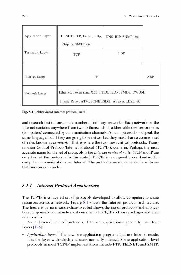
and research institutions, and a number of military networks. Each network on the

Internet contains anywhere from two to thousands of addressable devices or nodes

(computers) connected by communication channels. All computers do not speak the

same language, but if they are going to be networked they must share a common set

of rules known as protocols. That is where the two most critical protocols, Trans-

mission Control Protocol/Internet Protocol (TCP/IP), come in. Perhaps the most

accurate name for the set of protocols is the Internet protocol suite. (TCP and IP are

only two of the protocols in this suite.) TCP/IP is an agreed upon standard for

computer communication over Internet. The protocols are implemented in software

that runs on each node.

8.1.1 Internet Protocol Architecture

The TCP/IP is a layered set of protocols developed to allow computers to share

resources across a network. Figure 8.1 shows the Internet protocol architecture.

The figure is by no means exhaustive, but shows the major protocols and applica-

tion components common to most commercial TCP/IP software packages and their

relationship.

As a layered set of protocols, Internet applications generally use four

layers [1–5]:

• Application layer: This is where application programs that use Internet reside.

It is the layer with which end users normally interact. Some application-level

protocols in most TCP/IP implementations include FTP, TELNET, and SMTP.

Application Layer

Gopher, SMTP, etc.

Transport LayerTCP

Internet Layer ARP

Network Layer Ethernet, Token ring, X.25, FDDI, ISDN, SMDS, DWDM,

Frame Relay, ATM, SONET/SDH, Wireless, xDSL, etc

IP

UDP

TELNET, FTP, Finger, Http, DNS, RIP, SNMP, etc.

Fig. 8.1 Abbreviated Internet protocol suite

220 8 Wide Area Networks

For example, FTP (file transfer protocol) allows a user to transfer files to and

from computers that are connected to the Internet. Security is handled by

requiring the user to specify a user name and password for the other computer.

TELNET (network terminal protocol for remote login) allows a user to log on to

and use other computers that are connected to the Internet regardless of their

location. SMTP (simple mail transfer service; for computer mail) allows a user

to send messages to users on other computers. Originally, people tended to use

only one or two specific computers. They would maintain “mail files” on those

machines. The computer mail system is simply a way for you to add a message to

another user’s mail file.

• Transport layer: This layer controls the movement of data between nodes. The

layer provides communication services directly to the application processes

running on different hosts. The communication services may include the

multiplexing/demultiplexing function. In the Internet, there are two transport

protocols: TCP and UDP. TCP (Transmission Control Protocol) is connection-

oriented service that provides services needed by many applications. TCP also

provides segmentation of long messages and a congestion control mechanism.

UDP (User Datagram Protocol) provides connectionless services.

• Internet Layer: This handles addressing and routing of the data. It is also

responsible for breaking up large messages and reassembling them at the

destination. IP (Internet Protocol) provides the basic service of getting

datagrams to their destination. ARP (Address resolution protocol) figures out

the unique address of devices on the network from their IP addresses. The

Internet Protocol (IP) can be described as the common thread that holds the

entire Internet together. It is responsible for moving datagrams from one host to

another, using various techniques (or “routing” algorithms). Prior to transmitting

data, the network layer might subdivide or fragment it into smaller packets for

ease of transmission. When all the pieces finally reach the destination, they are

reassembled by the network layer into the original datagram.

• Network layer: This layer is responsible for routing datagrams from one host to

another. It contains the IP protocol as well as several routing protocols that

determine the routes of the datagrams. The network layer involves every host

and router in the network. It also supervises addressing and congestion control.

Protocols at this layer are needed to manage a specific physical medium, such as

Ethernet or a point-to-point line.

IP provides a connectionless, unreliable, best-effort packet delivery service.

Information is transferred as a sequence of datagrams. Those datagrams are treated

by the network as completely separate. For example, suppose we want to transfer a

15000 octet file. Most networks cannot handle a 15000 octet datagram. So the

protocols will break this up into something like 30 500-octet datagrams. Each of

these datagrams will be sent to the other end. At that point, they will be put back

together into the 15000-octet file. However, while those datagrams are in transit, the

network does not know that there is any connection between them. It is perfectly

possible that datagram 27 will actually arrive before datagram 19. It is also possible

8.1 Internet 221

that somewhere in the network, an error will occur, and some datagram would not

get through at all. In that case, that datagram has to be sent again.

As shown in Fig. 8.2, each layer of the protocol stack adds a header containing

layer-specific information to the data packet. A header for the network layer might

include information such as source and destination addresses. The process of

appending data with headers is called encapsulation. Figure 8.2 shows how data

is encapsulated by various headers. The reverse occurs during decapsulation: thelayers of the receiving stack extract layer-specific information and process the

encapsulated data accordingly. It is interesting to note that the process of encapsu-

lation increases the overhead involved in transmitting data. Although each of these

layers provides unique and valuable services, the Internet Protocol is perhaps the

most important to the overall operation of the Internet in general because it is

responsible for getting data from one host to another.

8.1.2 TCP Level

TCP puts a header at the front of each datagram. This header actually contains at

least 20 octets, but the most important ones are a source and destination “port

number” and a “sequence number.” The port numbers are used to keep track of

different conversations. Each datagram has a sequence number which is used so

that the other end can make sure that it gets the datagrams in the right order, and that

no datagrams are missing. Finally, the checksum is a number that is computed by

adding up all the octets in the datagram. The result is put in the header. TCP at the

other end computes the checksum again. If they disagree, then something bad

happened to the datagram in transmission, and it is thrown away. Figure 8.3

shows the datagram format.

Fig. 8.2 How data travels through the TCP/IP stack


Other items in the header are generally involved with managing the connection.

In order to make sure the datagram has arrived at its destination, the recipient has to

send back an “acknowledgement.” This is a datagram whose “Acknowledgement

number” field is filled in. For example, sending a packet with an acknowledgement

of 1500 indicates that you have received all the data up to octet number 1500. If the

sender does not get an acknowledgement within a reasonable amount of time, it

sends the data again. The “window” is used to control how much data can be in

transit at any one time. Each end indicates how much new data it is currently

prepared to absorb by putting the number of octets in its “Window” field. As the

computer receives data, the amount of space left in its window decreases. When it

goes to zero, the sender has to stop. As the receiver processes the data, it increases

its window, indicating that it is ready to accept more data. Often the same datagram

can be used to acknowledge receipt of a set of data and to give permission for

additional new data (by an updated window). The “Urgent” field allows one end to

tell the other to skip ahead in its processing of a particular octet.

8.1.3 IP level

IP (Internet Protocol) is the standard that defines the manner in which the network

layers of two hosts interact. All IP packets or datagrams consist of a header part and a

text part (payload). The payload has a maximum size limit of 65,536 bytes per

packet. The IP header consists of a 20-byte fixed part plus a variable part. Its size

is optimized to maximize the packet processing rate without utilizing excessive

resources. The header begins with a 4-bit version field that keeps track of the version

of the IP protocol to which the datagram belongs. This field helps smoothen the

transition from one version of IP to another, which can take months or even years.

IP packet contains a source and a destination address. The source address

designates the originating node’s interface to the network, and the destination

address specifies the interface for an intended recipient or multiple recipients (for

multicasting). These addresses are in the form of 32-bit binary strings.

Bit 0 31

Source Port (16) Destination Port (16)

Sequence Number (32)

Acknowledgement Number (32)

Flags(6) Window (16)

Checksum (16) Urgent Pointer (16)

Options (variable) Padding (variable)

Reserved(6)Data offset(4)

Fig. 8.3 TCP header format (20 bytes)

8.1 Internet 223

The header also consists of a Time to Live (TTL) that is used to limit the life of

the packet on the network. This is to take care of a situation in which an IP packet

gets caught in the system and becomes undeliverable. The TTL field maintains a

counter that is normally initialized to 30 count and is decremented each time the

packet arrives at a routing step. If the counter reaches zero, the packet is discarded.

TCP sends datagrams to IP with the Internet address of the computer at the other

end. IP’s job is simply to find a route for the datagram and get it to the other end. In

order to allow gateways or other intermediate systems to forward the datagram, it

adds its own header, as shown in Fig. 8.4. The main things in this header are the

source and destination Internet address (32-bit addresses, like 128.6.4.194), the

protocol number, and another checksum. The source Internet address is simply the

address of your machine. The destination Internet address is the address of the other

machine. The protocol number tells IP at the other end to send the datagram to TCP

or UDP or some other protocol. Although most IP traffic use TCP, there are other

protocols that can use IP, so you have to tell the IP which protocol to send the

datagram to. Finally, the checksum allows IP at the other end to verify that the

header was not damaged in transit. Note that TCP and IP have separate checksums.

IP needs to be able to verify that the header did not get damaged in transit, or it

could send a message to the wrong place. After IP has tacked on its header, the

message looks like what is in Fig. 8.4.

Conventionally IP addresses are usually written as four integers separated by

dots; each integer corresponding to 8 bits. For example, the binary address

10000000 00001011 00000110 00011110

is written in decimal form as

128.11.6.30

Thus, IP addresses are usually written as a sequence of four numbers separated

by three dots such as NNN.NNN.HHH.HHH, where N stands for octets that identify

network and H denotes octets that specify the host. Each number can be between

0 and 255 except the last number which must be between 1 and 254. Inside your

Bit 0 31

Version(4) IHL(4) Service type(8) Total length (16)

Identification (16) Flags(3) Fragment Offset (13)

Time to live (8) Protocol (8) Header Checksum (16)

Source Address (32)

Destination Address (32)

Options (variable) Padding (variable)

Fig. 8.4 IP header format (20 bytes)


computer, an IP address is stored as a 32 bit (4 byte) integer. Dotted decimal

notation is just an easy way for humans to write an IP address without having to

know the binary numbers that computers work with.

We all know that computers like to work with numbers, and humans prefer

names. With this in mind, the designers of the internet have set up a system to give

names to computers on the internet. A DNS Server is a computer somewhere that

can change a hostname into an IP address, and vice versa. It holds a database

similar to a telephone book. It also knows the address of other DNS servers it can

query if it does not have an entry for address you are looking for. For example,

when you ask your web browser to connect to www.yahoo.com, your computer

asks a DNS server to look up the IP address of www.yahoo.com. The DNS server

will tell your computer that it is 204.71.200.68. Your computer then uses that IP

address to contact yahoo.

IP handles complex networks the same way it handles small networks: one

hop at a time. Eventually, the datagrams will get through. This is illustrated in

Fig. 8.5, which shows different network segments in between the sending and

destination systems.

Most of today’s Internet uses Internet Protocol Version 4 (IPv4), which is now

nearly 25 years old. Due to the phenomenal growth of the Internet, the rapid

increase in palmtop computers, and the profusion of smart cellular phones and

PDAs, the demand for IP addresses has outnumbered the limited supply provided

by IPv4. In response to this shortcomings of IPv4, the Internet Engineering Task

Force (IETF) approved IPv6 in 1997. IPv4 will be replaced by Internet Protocol

Version 6 (IPv6), which is sometimes called the Next Generation Internet Protocol

(or IPng). IPv6 adds many improvements and fixes a number of problems in IPv4,

such as the limited number of available IPv4 addresses.

Fig. 8.5 A typical multi-hop network path

8.1 Internet 225

http://www.yahoo.com/

http://www.yahoo.com/

8.1.4 Performance Analysis

The Internet has some characteristics that make it exceedingly hard to analyze,

model or simulate. Such characteristics include its size, complexity, heterogeneity

of the subnetworks involved, and the fact that it changes drastically with time.

These difficulties have been tackled in different ways [6–11].

One way is to calculate the end-to-end delay. The end-to-end delay analysis will

involve the following components [6]:

• Packetization delay: This is time to fill an IP packet at the source. If we assume

that the source produces a constant bit stream, the packetization delay is the

payload size divided by the source information rate.

• Queueing delay: Packets have to be queued at every router since only one packetcan be processed at a time.

• Propagation delay: This is time taken by the packets to pass through the

transmission medium (copper or fiber).

Several other factors may contribute to the end-to-end delay but are usually not

significant.

Another way is to consider the end-to-end congestion control mechanism. It is

conventional to use packet drops as an indication of congestion. A conformant TCPconnection is one where the TCP sender follows the following two traits. First, the

TCP data sender interprets any packet drop in a window of data as an indication of

congestion, and responds by reducing the congestion window at least in half.

Second, during the congestion avoidance phase in the absence of congestion, the

TCP sender increases congestion control by at most one packet per round-trip time.

We say a flow is TCP-friendly when its arrival rate does not exceed the arrival rate

of a conformant TCP connection in the same circumstances. In order to be

TCP-friendly, the source’s average sending rate must not be higher than that

achieved by a TCP connection along the same path. Estimation of the steady state

throughput of a long-live TCP connection is given by

T ¼ k�MR�

ffiffiffipp (8.1)

where k ¼ constant of value 1.22 or 1.31 depending respectively on whether

delayed or nondelayed acknowledgement type is used

M ¼ maximum segment (packet) size

R ¼ round trip time experienced by the connection

p ¼ probability of loss during the life time of a connection

This simple formula assumes that the retransmission timeout never happens and

that packet loss occurs at random. In view of the current Internet, retransmission

timeout occurs as a result of network congestion and packet loss may not occur at

random. When the throughput estimation accounts for the retransmission timeout,

we obtain [7]


T ¼ M

Rffiffiffiffiffiffi2bp2

qþ 3To

ffiffiffiffiffiffi3bp8

qp 1þ 32p2ð Þ

(8.2)

where To ¼ retransmission timeout and b ¼ 2 (if delayed ACK is used or b ¼ 1

otherwise). From Eqs. (8.1) and (8.2), we notice that the throughput is inversely

proportional to the round trip time and the square root of the loss probability.

8.2 Broadband ISDN

The integrated services digital network (ISDN) is a facility which many claim to be

the most significant advance in telecommunications since the introduction of the

telephone itself. It is a digital end-to-end telecommunication wide area network

(WAN) in which voice, video, and data services are integrated. However, the

characteristics of narrowband ISDN are inadequate for many applications of inter-

est and in meeting the perceived users’ needs for higher speed, broader bandwidth,

and more flexibility such as video distribution, HDTV, and HiFi stereo. The needs

are accommodated in broadband ISDN (BISDN). Consequently, as far as data

networks are concerned, real excitement of ISDN comes about when one considers

the capabilities of BISDN [12].

Broadband is the provision of subscriber access at bit rates in excess of 2 Mbps.

Broadband applications are those implemented through broadband access and

require data rate greater than is generally available in narrowband ISDN. The

BISDN concept developed from the fact that a large range of voice, data, and

video services can be simultaneously carried on the same optical system. Broad-

band is the provision of subscriber access at bit rates in the range of 1.5 Mbps up to

approximately 150 Mbps. The demand for broadband communication originated

from business and residential customers. Residential customers are interested in

distribution services such as TV. Business customers require services for video,

data, and graphics. The bit rates for these services are in the range of 2–130 Mbps

and require broadband communication [13].

BISDN is regarded as an all-purpose digital network in that it will provide an

integrated access that will support a wide variety of applications in a flexible and

cost-effective manner.

8.3 Summary

1. The TCP/IP has been the foundation of the Internet and virtually all multivendor

internetworks. They are the world’s most popular open-system (nonproprietary)

protocol suite because they can be used to communicate across any set of

interconnected networks and are equally suited for LAN, MAN, and WAN

communications.

8.3 Summary 227

2. BISDN started out as an extension of ISDN and has many concepts similar

to ISDN.

More about WAN can be found in [14] and its performance analysis is

presented in [15].

Problems

8.1 It is called TCP/IP. Mention three other protocols in the suite and what they

are for.

8.2 What is the difference between TCP and UDP if they both operate at

the transport layer?

8.3 What are the layers of the TCP/IP model and how are they related to the

OSI model?

References

1. J. Crowcroft, “The Internet: a tutorial,” Electronics & Communication Engineering Journal,June 1996, pp. 113-122.

2. M. R. Arick, The TCP/IP Companion: a guide for the common user. Boston, QED Publishing

Group, 1993.

3. U. Black, TCP/IP and Related protocols. New York: McGraw-Hill, 2nd ed., 1995.

4. J. Martin, TCP/IP Networking: Architecture, Administration, and Programming. EnglewoodCliffs, NJ: Prentice Hall, 1994.

5. D. M. Peterson, TCP/IP Networking: a guide to the IBM environment. New York: McGraw-

Hill, 1995.

6. S. Floyd and K. Fall, “Promoting the use of end-to-end congestion control in the Internet,”

IEEE/ACM Transactions on Networking, vol. 7, no. 4, Aug. 1999, pp. 458-472.7. S. Hassan and M. Kara, “Performance evaluation of end-to-end TCP-friendly video traffic in

the Internet,” Proceeding of 9th IEEE International Conference on Networks, 2001, pp. 56-61.8. K. Van der Wal et al., “Delay performance analysis of the new Internet services with

guaranteed QoS,” Proceedings of the IEEE, vol. 85, no. 12, Oct. 1997, pp. 1947-1957.9. S. Floyd and V. Paxson, “Difficulties in simulating the Internet,” IEEE/ACM Transactions on

Networking, vol. 9, no. 4, Aug. 2001, pp. 392-403.10. J. W. Roberts, “Traffic theory and the Internet,” IEEE Communications Magazine, Jan. 2001,

p. 94-99.

11. J. A. Schormans et al., “Buffer overflow probability for multiplexed on-off VoIP sources,”

Electronics Letters, vol 36, no. 6, March 2000, pp. 523-524.

12. L. Kleinrock, “ISDN – The Path to Broadband Networks,” Proceedings of the IEEE,vol. 79, no. 2, Feb. 1991, pp. 112-117. Also in [14], pp. 151-156.

13. R. Y. Awdeh, “Why Fast Packet Switching?” IEEE Potential, April 1993, pp. 10-12.14. M. N. O. Sadiku and S. M. Musa, Computer Communication for Metropolitan and Wide Area

Networks. New York: Nova Science Publishers, 2010.

15. S. V. Subramanian and R. Dutta, “Performance measurements and analysis of M/M/c queuing

model based SIP proxy servers in local and wide area networks,” Proc. of 2010 InternationalConference on Advances in Recent Technologies in Communication and Computing, 2010,pp. 306-310.


Chapter 9

Wireless Networks

What you do speaks so loudly that I cannot hear what you say.

—Ralph Waldo Emerson

Wireless communications is one of the fastest growing fields in engineering. The

last century has witnessed the introduction of many kinds of wireless networks,

some of which have become the cornerstone of modern life. Such networks have

provided support for nomadic and increasingly mobile users.

Wireless networks evolve around new and old technologies. Such networks

include [1]:

• Wireless local area networks (WLANs), which enable communication between

stations without cables by means of radio frequency or infrared

• Wireless local loop (WLL) or fixed radio, which provides telephone, fax, and

data services

• Wireless private branch exchanges (WPBXs), which facilitate communication

with the office environment, allowing workers to roam

• Wireless personal area network (WPAN), which refers to using a near-field electric

field to send data across various devices using the human body as a medium

• Wireless personal communications services (PCS), which describe all access

technologies used by individuals or subscribers

• Cellular communications, which allows frequency reuse by dividing regions into

small cells, each cell with a stationary radio antenna

• Satellite communications, which uses orbiting satellites to relay data between

multiple earth-based stations.

The performance analysis of wireless networks is more complicated than that for

fixed networks because we must take into account a lot of parameters such as the

cell number, buffer size, and user mobility. For this reason, most performance

analyses use simulation and very few provide close form solution. In this chapter,

we consider ALOHA network, wireless LAN, and wireless MAN.


229

9.1 ALOHA Networks

ALOHA is the simplest broadcast protocol. The original goal of ALOHA was to

investigate the use of radio communications as an alternative to the telephone

system for computer networks. At that time, the University of Hawaii was com-

posed of six campuses on different islands all within a radius of 300 km from the

main campus near Honolulu. It was envisaged that such a radio data network would

connect these campuses and allow sharing of computer resources [2]. Thus,

ALOHA networks were proposed to make short delays possible. They are random

time-division multiple access networks because stations or terminals make use of

the channel at random times. The principles of ALOHA systems are incorporated in

both LANs and WANs. For example, ALOHA-based protocols are used in CSMA/

CD and token ring, which are LANs. They are also used in VSAT networks, which

are WANs [3].

In a pure ALOHA network, all users can initiate transmission at any time, in

completely unsynchronized manner. Any station which has a packet to transmit

simply transmits the packet regardless of whether other stations are transmitting. If,

within some appropriate time-out period, an acknowledgement is received from the

destination, the transmission is regarded successful. A transmission is unsuccessful

if no acknowledgement is received after a certain time. The station will then assume

its packet is lost. Through a random process, the station will determine a certain

waiting time and retransmit the packet when that time expires.

A useful performance characteristic for ALOHA network is the relationship

between throughput S and offered load G. Assume that the start times of packets in

the channel comprise a Poisson point process with parameter λ packets/s so that

Prob k arrivals in τ seconds½ � ¼ λτð Þkk!

e�λτ (9.1)

If each packet lasts τ seconds, we define the normalized channel traffic G as

G ¼ λτ (9.2)

We may assume that only those packets which do not overlap with other packets

are correctly received. We define the normalized channel throughput S as

S ¼ GPs (9.3)

where Ps is the probability that an arbitrary offered packet is successful. The

probability that a packet will not overlap a given packet is the probability that no

packet starts τ seconds before or τ seconds after the start time of the given packet

(i.e. a vulnerable interval of 2τ). Since the start times constitute a Poisson point

process, the probability of having no packet overlap is obtained using Eq. (8.1), i.e.

Ps ¼ Prob 0 arrivals in 2τ seconds½ � ¼ e�2λτ ¼ e�2G (9.4)

230 9 Wireless Networks

http://dx.doi.org/10.1007/978-3-319-01646-7_8#Equ1

Thus,

S ¼ Ge�2G (9.5)

The pure ALOHA achieves a maximum throughput of 1/(2e) ¼ 0.184 at

G ¼ 0.5.

Subsequently, a modified scheme was proposed in which the time axis is

segmented into time slots. In this slotted ALOHA, users are still allowed to transmit

randomly but a packet needs to be of fixed length and it must fall exactly in one of

the time slots. If two packets overlap, they overlap completely rather than partially

(i.e. a vulnerable interval of only τ). Hence,

S ¼ Ge�G (9.6)

With this simple change, the maximum throughput is increased by a factor of

2 to 1/e ¼ 0.368 at G ¼ 1. This implies that on the average, 36.8 % of the slots are

successfully transmitted, 36.8 % are idle, while the rest of the slots contain

collisions. The slotted version reduces frequencies of collisions and thereby

increases the maximum throughput of the random-access channel.

An example of the slotted ALOHA is in GSM cellular networks. Another

application of slotted ALOHA is in very small aperture terminal (VSAT), which

a satellite network in which small terminals are geographically widespread.

ALOHA is also used in wireline networks [3].

A comparison of both pure and slotted ALOHA is made in Fig. 9.1. It is not

possible to have a stable point of operation for G > 0.5 for pure ALOHA or

G > 1.0 for slotted ALOHA [4].

Fig. 9.1 Throughput versus offered load for pure and slotted ALOHA

9.1 ALOHA Networks 231

Example 9.1 Suppose an ALOHA network employs a 4.8-kbps channel for sending

packets which are each 200 bits. What is the maximum throughput possible for pure

and slotted ALOHA?

Solution

The system transmits packets at the rate of

4,800 bits/s � 1 packet/200 bits ¼ 24 packets/s

For pure ALOHA, the maximum possible throughput is

24� 0:184 � 4 packets=s

For slotted ALOHA, the maximum possible throughput is

24� 0:368 � 8 packets=s

9.2 Wireless LAN

Wireless local area network (WLAN) is a new form of communication system. It is

basically a local area network, confined to a geographically small area such as a

single building, office, store or campus, that provides high data connectivity to

mobile stations. Using electromagnetic airwaves (radio frequency or infrared),

WLANs transmit and receive data over the air. A WLAN suggests less expensive,

fast, and simple network installation and reconfiguration.

The proliferation of portable computers coupled with the mobile user’s need for

communication is the major driving force behind WLAN technology. WLAN

creates a mobile environment for the PC and LAN user. It may lower LAN

maintenance and expansion costs since there are no wires that require reconfigura-

tion. Thus, WLANs offer the following advantages over the conventional wired

LANs:

• Installation flexibility: allows the network to go where wire cannot go.

• Mobility: can provide LAN users with access anywhere.

• Scalability: can be configured in a variety of topologies to meet specific needs.

However, WLAN does not perform as well as wired LAN because of the

bandwidth limitations and may be susceptible to electromagnetic interference.

While the initial investment on WLAN hardware can be higher than the cost of

wired LAN hardware, overall installation expenses and life-cycle costs can be

significantly lower.


9.2.1 Physical Layer and Topology

WLAN does not compete with wired LAN. Rather, WLANs are used to extend

wired LANs for convenience and mobility. Wireless links essentially fill in for

wired links using electromagnetic radiation at radio or light frequencies between

transceivers. A typical WLAN consists of an access point and the WLAN adapter

installed on the portable notebook. The access point is a transmitter/receiver

(transceiver) device; it is essentially the wireless equivalent of a regular LAN

hub. An access point is typically connected with the wired backbone network at a

fixed location through a standard Ethernet cable and communicates with wireless

devices by means of an antenna. WLANs operate within the prescribed 900 MHz,

2.4 GHz, and 5.8 GHz frequency bands. Most LANs use 2.4 GHz frequency bands

because it is most widely accepted.

A wireless link can provide services in several ways including the following

three [5]:

• Replace a point-to-point connection between two nodes or segments on a LAN.

A point-to-point link is a connection between two devices for transferring data.

A wireless link can be used to bridge two LAN segments. Like a point-to-point

link, the link connects two wireless bridges attached to the two LANs. Such an

arrangement is useful for linking LANs in two buildings where a highway or

river makes direct connection difficult.

• Provide a connection between a wired LAN and one or more WLAN nodes.

In this case, a device is attached to the wired LAN to act as a point of contact

(called access point) between the wired LAN and the wireless nodes as shown in

Fig. 9.2. The device can be a repeater, bridge or router.

• Act as a stand-alone WLAN for a group of wireless nodes. This can be achieved

using topologies similar to wired LAN, namely, a star topology can be formed

with central hub controlling the wireless nodes, a ring topology with each

wireless node receiving or passing information sent to it or a bus topology

with each wireless capable of hearing everything said by all the other nodes.

9.2.2 Technologies

When designing WLANs, manufacturers have to choose from two main

technologies that are used for wireless communications today: radio frequency

(RF) and infra red (IR). Each technologies has its own merits and demerits.

RF is used for applications where communications are over long distances and

are not line-of-sight. In order to operate in the license free portion of the frequency

spectrum known as the ISM band (Industrial, Scientific, and Medical), the RF system

must use a modulation technique called spread spectrum (SS). (SS was used in

IEEE 802.11b.) Spread spectrum is wideband radio frequency technology developed

by the military during World War II for use in reliable, secure, mission-critical

9.2 Wireless LAN 233

communications systems. SS system is one in which the transmitted signal is spread

over frequency much wider than the minimum bandwidth required to send the signal.

Using spread spectrum, a radio is supposed to distribute the signal across the entire

spectrum. This way, no single user can dominate the band and collectively all users

look like noise. The fact that such signals appear like noise in the band makes them

difficult to find and jam, thereby increasing security against unauthorized listeners.

There are two types of spread spectrum technology: frequency hopping and direct

sequence.

Frequency hopping spread spectrum (FHSS) offers a current maximum data rate

of 3 Mbps. It uses a narrowband carrier that changes frequency in a pattern known

to both transmitter and receiver. It is based on the use of a signal at a given

frequency that is constant for a small amount of time and then moves to a new

frequency. The sequence of different channels for the hopping pattern is determined

in pseudorandom fashion. This means that a very long sequence code is used before

it is repeated, over 65,000 hops, making it appear random. Thus it is very difficult to

predict the next frequency at which such a system will stop and transmit/receive

data as the system appears to be a noise source to an unauthorized listener. This

makes FHSS system very secure against interference and interception.

Direct sequence spread spectrum (DSSS) takes a signal at a given frequency and

spreads it across a band of frequencies where the center frequency is the original

signal. The spreading algorithm, which is the key to the relationship of the spread

range of frequencies, changes with time in a pseudorandom sequence. When the

ratio between the original signal bandwidth and the spread signal bandwidth is very

large, the system offers great immunity to interference. For example, if 10 kbps

signal is spread across 1 GHz of spectrum, the spreading ratio is 100,000 times or

Nodes on wired Ethernet

WirelessAccess Point/

Bridge

Wireless Nodes

Fig. 9.2 Connection of a wired LAN to wireless nodes


50 dB. However, in the ISM band used inWLAN, the available bandwidth critically

limits the ratio of spreading and so the advantages of DSSS scheme against

interference is greatly limited. It has been shown that for the WLAN system

using DSSS, the spreading ratio is at best ten times. DSSS is characterized by

high cost, high power consumption, and more range than FHSS and infrared

physical layers. FHSS is characterized by low cost, low power consumption, and

less range than DSSS but greater range than infrared. Most WLAN systems

use FHSS.

The second technology used in WLAN is Infra Red (IR), where the communi-

cation is carried by light in the invisible part of the spectrum. It is primarily used for

very short distance communications (less than 1 m), where there is a line-of-sight

connection. Since IR light does not penetrate solid materials (it is even attenuated

greatly by window glass), it is not really useful in comparison to RF in WLAN

system. However, IR is used in applications where the power is extremely limited

such as a pager.

9.2.3 Standards

Although a number of proprietary, non-standard wireless LANs exist, standards

have now been developed. Two international organizations have contributed to the

development of standards for WLANs: the Institute of Electronics and Electrical

Engineers (IEEE) and the European Telecommunications Standards Institute

(ETSI). Mainly it is IEEE for 902.11; ETSI is involved in cellular.

In 1997, the IEEE 802.11 committee (http://ieee802.org/11) issued a standard

for wireless LANs. The standard addresses the physical and MAC layers of the OSI

model and includes the following [5, 6]:

• A transmission rate of up to 2 Mbps

• Two different media for transmission over wireless LAN: infrared (IR) and radio

frequency (RF)

• The media access control (MAC) protocol as carrier sense multiple access with

collision avoidance (CSMA/CA), i.e. devices can interoperate with wired LANs

via a bridge

• MAC protocol provides two service types: asynchronous and synchronous

(or contention-free). The asynchronous type of service is mandatory while the

synchronous type is optional

• MAC layer protocol is tied to the IEEE 802.2 logical link control (LLC) layer

making it easier to integrate with other LANs

• Three different physical layers: an optical-based physical-layer implementation

that uses IR light to transmit, two RF based physical-layer choices: direct

sequence spread spectrum (DSSS) and frequency hopping spread spectrum

(FHSS) both operating at 2.4 GHz industrial, scientific, and medical (ISM)


http://ieee802.org/11

frequency bands. (The ISM bands 902–928 MHz, 2,400–2,483.5 MHz, and

5,725–5,850 MHz do not require a license to operate.) The IEEE 802.11

specifications for DSSS wireless LAN is shown in Fig. 9.3.

• Added features to the MAC that can maximize battery life in portable clients via

power-management schemes.

• Data security through which the wireless LANs can achieve wired equivalent

privacy.

The standard basically defines the media and configuration issues, transmission

procedures, throughput requirements, and range characteristics for WLAN technol-

ogy. It avoids rigid requirements and gives room for vendors in the following areas:

multiple physical media, common MAC layer irrespective of the physical layer,

common frame format, power limit, and multiple on-air data rates [7].

There are three major problems encountered by an RF LAN [8]. First, frequency

allocation is limited for LANs. But since LANs operate with low power, frequency

reuse is possible. Second, interference from other wireless LANs controlled

by different organization and other wireless sources is a problem. This problem

can be controlled by using spread spectrum techniques. Third, security is at stake

because RF signal can penetrate through the wall and hostile operators can intercept

RF LAN communications. Encryption can be used to lessen this problem. IR LAN

uses both laser diodes and light-emitting diodes as emitters. It is useful in high

electromagnetic interference (EMI) environments. It is also secure since IR signal

cannot penetrate the wall.

Channel 1

2.401 2.412 2.423

Channel 7

2.431 2.442 2.453

Channel 2

2.406

2.433

2.428

Channel 3

Channel 8

Channel 9

Channel 4

2.411

2.436 2.447 2.458

2.422

2.417

2.441 2.452 2.463 Channel 10

Channel 5 2.416 2.427 2.438 2.446 2.457 2.468

2.421 2.432 2.443 2.451 2.462

2.426 2.448

2.473

2.437

Channel 11

Channel 6

Fig. 9.3 Eleven 22-MHz-wide channels for DSSS wireless LANs


CSMA/CA is slightly different from carrier sense multiple access with collision

detection (CSMA/CD), which is the MAC protocol used in Ethernet wired LAN. In

CSMA/CA, when a node has something to transmit, it waits for silence on the

network. When no other nodes are heard, it transmits and waits to receive an

acknowledgement from the recipient node. If it fails to receive an acknowledge-

ment within a time period, it assumes that collision has occurred and follows a

process similar to CSMA/CD. Each node then waits for silence and only transmits

after a random amount of waiting. While CSMA/CA protocol is slower that CSMA/

CD due to the need for waiting for acknowledgement, it works well for wireless

LANs. Also, WLANs operate in strong multipath fading channel where channel

characteristics can change resulting in unreliable communication.

The ETSI devoted its attention to RF wireless LANs. The ETSI is close to

finalizing its standard, which is based on the 2.4 GHz range used for spread-

spectrum LANs in several European countries. European standard WLAN, called

HiperLAN, will allow speeds of 24 Mbps [9].

Besides IEEE and ETSI, there are organizations that are more interested in the

implementation and interoperability of WLAN products. Such organizations

include Wireless LAN Alliance (WLANA at www.wlana.com) and Wireless Ether-

net Compatibility Alliance (WECA at www.wi-fi.org or www.wirelessethernet.

com). WLANA was formed in 1996 with 12 members as a trade association for

wireless LAN vendors. WECA is a nonprofit manufacturing consortium with over

60 companies as members; it was formed in 1999 to certify interoperability of IEEE

802.11 products. Research groups are working hard to shrink radios into a chip that

can be mass produced cheaply. If they succeed, the demand for radio LANs may

follow the same trend as cellular phones in recent years.


We now present an accurate but simple analytical evaluation of the wireless

networks using gated and exhaustive polling protocols combined with the stop-

and-wait or go-back-N automatic repeat request (ARQ) techniques. In gated access

policy, upon receiving a polling message, a station is permitted to transmit all

packets stored in its buffer until that time. For the exhaustive policy, a station upon

receiving a polling message is permitted to transmit all packets in its buffer as well

as packets arriving while transmitting.

Assuming that the transmission system is completely symmetric, the average

packet waiting time for gated policy is (in slots)

Wg ¼ 1

2

Nλt2

1� Nλtþ 1þ λtð ÞNR

1� Nλtþ R2

R� R � 1

!þ t � 1 (9.7)


http://www.wlana.com/

http://www.wi-fi.org/

http://www.wirelessethernet.com/

http://www.wirelessethernet.com/

where λ is the arrival rate; N is the number of stations; t is the packet transmission

time with first moment t and second moment t2 ; R is the walk time with first

moment R and second moment R2 . For exhaustive policy, the corresponding

equation is

We ¼ 1

2

Nλt2

1� Nλt2þ 1� λtð ÞNR

1� Nλtþ R2

R� R � 1

!þ t � 1 (9.8)

The above analysis has been presented in a summarized form. For more details,

the interested reader is referred to [10, 11].

The above model is on a general WLAN. We now consider an IEEE 802.11

based WLAN, where the nodes use Distributed Coordination Function (DCF) mode

of the MAC protocol. We recall that DCF is governed by a “listen-before-talk”

protocol known as CSMA. Every station that wants to transmit first senses the

channel for at least a duration of DIFS (Distributed Inter Frame Spacing). If the

channel is idle for the entire DIFS, the station transmits the packet. Otherwise, it

avoids collision by selecting a random back-off time uniformly distributed in the

range [0, CW], where CW is the Contention Window. Under saturation conditions,

the CSMA/CA process can be modeled as a two dimensional Markov chain.

We now can express the probability τ that a station transmits in a randomly

selected slot time. Let p be the probability that its transmission will collide with at

least one other node. In [12–14], the access probability τ is related to the collision

probability of each packet p as

τ ¼ 2 1� 2pð Þ1� 2pð Þ W þ 1ð Þ þ pW 1� 2pð Þm½ � (9.9)

where W is the minimum backoff window in terms of backoff slots, and m is the

maximum backoff stage. Notice from Eq. (9.9) that when m ¼ 0, i.e. no exponen-

tial backoff is considered,

τ ¼ 2

W þ 1(9.10)

i.e. τ is independent of p. However, τ generally depends on the collision

probability p, which is yet to be found. To find p. we note that p is the probability

that, in a time slot, at least one the n � 1 remaining stations transmits

p ¼ 1� 1� τð Þn�1 (9.11)

Equations (9.9) and (9.11) together form a system of nonlinear system and need

to solved using numerical techniques (e.g. Newton’s method). Once τ is known, wecan calculate the throughput.


Let S be the normalized system throughput, defined as the fraction of time the

channel is used to successfully transmit. Let Ptr be the probability that there is at

least one transmission in the considered slot time. Since n stations contend for

transmission and each transmit with probability τ:

Ptr ¼ 1� 1� τð Þn (9.12)

The probability Ps that a transmission is successful is

Ps ¼ nτ 1� τð Þn�1Ptr

¼ nτ 1� τð Þn�11� 1� rð Þn (9.13)

We now express the throughput S as the ratio

S ¼ E payload information transmitted in one slot time½ �E length of a slot time½ � (9.14)

If E[P] is the average packet payload size, the average amount of payload

information successfully transmitted in a slot time is PtrPsE[P], since a successfultransmission occurs in a slot time with probability PtrPs. Hence, Eq. (9.14) becomes

S ¼ PsPtrE P½ �1� Ptrð Þσ þ PtrPsTs þ Ptr 1� Psð ÞTc

(9.15)

Where σ is the duration on an empty slot time, Ts is the average time the channel

is senses busy because of a successful transmission, and Tc is the average time the

channel is sensed busy by each node during a collision.

Other models on performance analysis of WLAN and WMAN can be found in

[15–17].

9.3 Multiple Access Techniques

Since spectrum is a scarce and limited resource, multiple access schemes are

designed to share the resource among a large number of wireless users. There are

three popular multiple-access techniques for sharing the available bandwidth in a

wireless communication system:

• The frequency division multiple access (FDMA) serves users with different

frequency channels. Signals are transmitted in nonoverlapping frequency

bands that can be separated using bandpass filters.

• The time division multiple access (TDMA) serves users with different time slots.

Signals are transmitted in nonoverlapping time slots in a round-robin fashion.

In each slot only one user is allowed to either transmit or receive.

9.3 Multiple Access Techniques 239

• The code division multiple access (CDMA) serves users with different code

sequences. Different users employ signals that have small cross-correlation.

The three access methods are portrayed in Fig. 9.4. In addition to FDMA,

TDMA, and CDMA, there are other two multiple access schemes—polarization

division multiple access (PDMA) which serves users with different polarization and

space division multiple access (SDMA) which controls the radiated energy for users

in space by using spot beam antenna [18].

9.3.1 FDMA, TDMA, and CDMA

FDMA requires that the total bandwidth be divided into a number of disjoint

frequency subchannels. Each subchannel is assigned on demand to individual

users who request service. As shown in Fig. 9.4, guard bands are maintained

FDMA TDMA

CDMA (FH)

User 1

a

c

b

User 2

User 3

Guard Band

Guard Band

Time

Frequency

User 1 User 2 User 3

Time

Frequency

Guard Time

User 1

User 2

User 3

User 2

User 3

User 1

User 3

User 1

User 2

Time

Frequency

Fig. 9.4 Multiple access techniques for wireless systems


between adjacent spectra to minimize cross talk between channels. The present FM

radio subdivides the spectrum into 30-kHz channels so that each channel is assigned

to one user. In FDMA, the 30-kHz channel can be split into three 10-kHz channels.

This band-splitting, however, incurs costs. For reasons of spectral efficiency, the

transmission rate on a single FDMA channel is usually close to the maximum rate

required by the user. Consequently, FDMA is suitable for users with nonbursty and

predictable traffic. Cellular networks do not use FDMA by itself anymore. That

passed with first generation networks. TDMA, at least in cellular, is used with

FDMA. TDMA and CDMA can support more users in the space spectrum region.

The GSM air interface uses a mixture of FDMA and TDMA.

TDMA is a channelization scheme that triples the capacity of the available

channels without requiring additional RF spectrum. A frame consists of a number

of time intervals called slots. As shown in Fig. 9.5, each TDMA frame consists of a

preamble, information message, and trail bits. The preamble has the address and

synchronization information that both the base station and the subscribers will use to

identify each other. Guard times are used between slots to minimize cross talk. One

downside of TDMA is that the high rate switching/multiplexing of the time-domain

transmission signals places stringent requirements on the analog components follow-

ing the modulator.

CDMA is a spread spectrum technique in which the narrowband signal from

each user is spread out in frequency using a unique spreading code. Several signals

may occupy the same frequency band and still be individually recovered by the

receiver with the knowledge of the spreading code. Each user operates indepen-

dently of other users. Each user is assigned a unique code sequence that he uses to

encode his information signal. The receiver, fully aware of the code sequence of the

user, decodes the received signal after reception and recovers the original data.


In this section, we develop some analytical models to provide insights into the

characteristics of FDMA and TDMA systems [19]. Suppose N users, each with

infinite buffer size, transmit packets of constant length L bits. The packet arriving

One TDMA frame

Preamble Information Message Trail Bits

Slot 1 Slot 2 Slot 3 * * * *

Trail Bits Sync. Bits Information Data Guard Bits

Slot N

Fig. 9.5 TDMA frame

structure

9.3 Multiple Access Techniques 241

rate is λ packets/s. For TDMA, packets are transmitted using the full channel

bandwidth of NR bps, while FDMA systems transmit at R bps.

9.3.2.1 Frequency Division Multiple Access

The queueing model is shown in Fig. 9.6.

Using the result of M/G/1 queueing model, the waiting time is

E Wð Þ ¼ λE2 Sð Þ2 1� ρð Þ ¼

λ LR=N

� �22 1� ρð Þ ¼

λN2L2

2R2 1� ρð Þ (9.16)

The overall delay is

E Dð Þ ¼ E Wð Þ þ E�S�

¼ λN2L2

2R2 1� ρð Þ þNL

R(9.17)

For the queue to be stable with finite delay,

ρ ¼ λE Sð Þ ¼ λNL

R< 1 (9.18)

9.3.2.2 Time Division Multiple Access

The delay in TDMA comprises of two components: (a) waiting time for the start of

the time slot, (b) waiting time for packets that arrived earlier in the same queue to be

transmitted. Using the result of M/G/1 queue,

λ R/N

.

.

.

λ R/N

Fig. 9.6 Queueing model

of FDMA


E Wð Þ ¼ λE2 Sð Þ2 1� ρð Þ þ

E S2� �

2E Sð Þ

¼λ

L

R=N

0@

1A2

2 1� ρð Þ þ

L

R=N

0@

1A2

2L

R=N

0@

1A

¼ λN2L2


2R

(9.19)

The second term represents the fact that on the average, an arriving packet has to

wait half the frame length (NL/R) before it is transmitted in its own time slot. The

overall delay is

E Dð Þ ¼ E Wð Þ þ L

R

¼ λN2L2


2Rþ L

R

(9.20)

Note that

E Wð ÞTDMA ¼ E Wð ÞFDMA þNL

2R> E Wð ÞFDMA (9.21)

E Dð ÞTDMA ¼ E Dð ÞFDMA þL

R� NL

2R(9.22)

i.e.

E Dð ÞFDMA > E Dð ÞTDMA !NL

2R� L

R> 0! N > 2 (9.23)

This indicates that in terms of performance TDMA is superior to FDMA because

the packet delay in FDMA is typically larger than TDMA. For three or more users,

the overall delay in FDMA is greater than TDMA.

9.4 Cellular Communications

Perhaps no single development has done more for wireless technologies than has

cellular communications. It is one of the fastest growing and most demanding

telecommunication applications. It has been predicted that cellular will be the

universal method of personal communication.

9.4 Cellular Communications 243

9.4.1 The Cellular Concept

The cellular concept is not so much a new technology as it is a new idea of

organizing old technology. It was developed in 1947 at Bell Laboratories; the

first cellular system began operation in Japan in 1979, and the first cellular system

in the U.S. began in October, 1983 in Chicago. The first generation of cellular

systems was based on analog FM radio technology. The second-generation cellular

systems are based on digital radio technology and conform to at least three

standards: GSM for Europe and international applications, AMPS for the U.S.,

and JDC for Japan. Third-generation cellular systems use TDMA, CDMA, CSMA,

and FDMA.

The conventional approach to mobile radio involved setting up a high-power

transmitter on top of the highest point in a coverage area. The mobile telephone had

to have a line-of-sight to the base station for proper coverage. Line-of-sight

transmission is limited to as much as 40–50 miles on the horizon. Also, if a mobile

travels too far from the base station, the quality of the communications link

becomes unacceptable. These and other limitations of conventional mobile tele-

phone systems are overcome by cellular technology.

Areas of coverage are divided into small hexagonal radio coverage units known

as cells. (The hexagonal shape is only for the sake of illustration; the shapes of

real cells are irregular.) A cell is the basic geographical unit of a cellular system.

A cellular communications system employs a large number of low-power wireless

transmitter, as shown in Fig. 9.7.

Cells are base stations transmitting over small geographical areas that are

represented as hexagons. Cell size varies depending on the landscape and tele-

density. Each side typically covers a maximum area of 15 miles across, depending

on the local terrain. Urban cells are smaller for reuse. The cell sites are spaced over

the area to provide a slightly overlapping blanket of coverage. Like the early mobile

Fig. 9.7 A typical wireless

seven-cell patterns; cells

overlap to provide greater

coverage


systems, the base station communicates with mobiles via a channel. The channel is

made of two frequencies: the forward link for transmitting information to the base

station and the reverse link to receive from the base station.

9.4.2 Fundamental Features

Besides the idea of cells, the essential principles of cellular systems include cell

splitting, frequency reuse, hand-off, capacity, spectral efficiency, mobility, and

roaming [1, 20].

• Cell splitting: As a service area becomes full of users, the area is split into small

ones. Consequently, urban regions with heavy traffic can be split into as many

areas as necessary to provide acceptable service, while a large cell can be used to

cover remote rural regions. Cell splitting increases the capacity of the system.

• Frequency reuse: This is the core concept that defines the cellular system. The

cellular-telephone industry is faced with a dilemma: services are growing

rapidly and users are demanding more sophisticated call-handling features, but

the amount of the electromagnetic spectrum allocation for cellular service is

fixed. This dilemma is overcome by the ability to reuse the same frequency

(channel) many times. Several frequency reuse patterns are in use. A typical

example is shown in Fig. 9.8, where all available channels are divided into

6 1,13,20

3 3,10,17

6 6,13,20

3 3,10,17

4 4,11,18

1 1,8,15

5 5,12,19

4 4,11,18

1 1,8,15

5 5,12,19

5 5,12,19

2 2,12,19

2 2,12,19

2 2,12,19

2 2,12,19

2 2,12,19

2 2,12,19

3 3,10,17

3 3,10,17

3 3,10,17

3 3,10,17

3 3,10,17

5 5,12,19

5 5,12,19

5 5,12,19

5 5,12,19

7 7,14,21

7 7,14,21

7 7,14,21

7 7,14,21

7 7,14,21

7 7,14,21

7 7,14,21

4 4,11,18

6 6,13,20

6 6,13,20

6 6,13,20

6 6,13,20

6 6,13,20

4 4,11,18

4 4,11,18

4 4,11,18

4 4,11,18

1 1,8,15

2 2,12,19

1 1,8,15

1 1,8,15

1 1,8,15

1 1,8,15

Fig. 9.8 Frequency reuse in a seven-cell pattern cellular system


21 frequency groups numbered 1–21. Each cell is assigned three frequency

groups. For example, the same frequencies are reused in the cell designated as

1 and adjacent locations do not reuse the same frequencies. A cluster is a group

of cells; frequency reused does not apply to clusters.

• Hand-off: This is another fundamental feature of the cellular technology. When a

call is in progress and the switch from one cell to another becomes necessary, a

hand-off takes place. Hand-off is important, because adjacent cells do not use the

same radio channels as a mobile user travels from one cell to another during a

call, the call must be either dropped (blocked) or transferred from one channel to

another. Dropping the call is not acceptable. Hand-off was created to solve the

problem. Handing off from cell to cell is the process of transferring the mobile

unit that has a call on a voice channel to another voice channel, all done without

interfering with the call. The need for hand-off is determined by the quality of

the signal, whether it is weak or strong. A hand-off threshold is predefined.

When the received signal level is weak and reaches the threshold, the system

provides a stronger channel from an adjacent cell. The hand-off process

continues as the mobile moves from one cell to another as long as the mobile

is in the coverage area. A number of algorithms are used to generate and process

a hand-off request and eventual hand-off order.

• Mobility and roaming: Mobility implies that a mobile user while in motion will

be able to maintain the same call without service interruption. This is made

possible by the built-in hand-off mechanism that assigns a new channel when the

mobile moves to another cell. Because several cellular operators within the same

region use different equipment, and a subscriber is registered with only one

operator, some form of agreement is necessary to provide services to

subscribers. Roaming is the process whereby a mobile moves out of its own

territory and establishes a call from another territory.

• Capacity: This is the number of subscribers that can use the cellular system. For

a circuit-switched system, the capacity is determined by the loading (number of

calls and the average time per call). Capacity expansion is required because

cellular system must serve more subscribers. It takes place through frequency

reuse, cell splitting, planning, and redesigning of the system.

• Spectral efficiency: This is a performance measure of the efficient use of the

frequency spectrum. It is the most desirable feature of a mobile communication

system. It produces a measure of how efficiently space, frequency, and time are

utilized. Expressed in channels/MHz/km2, channel efficiency is given by

η ¼ Total no: of channels available in the system

Bandwidth� Total coverage area(9.24)

η ¼Bw

Bc� Nc

N

Bw � Nc � Ac¼ 1

BcNAc(9.25)


where Bw is bandwidth of the system in MHz, Bc is the channel spacing in MHz,

Nc is the number of cells in a cluster, N is the frequency reuse factor of the

system, and Ac is the area covered by a cell in km2.


There are two common performance indices used in designing cellular systems

[21, 22]. The first index is the call blocking probability, which is the probability thata new, originating call is denied due to the unavailability of free channels. The

second index is the call dropping probability of hand-off call, which is the proba-

bility that an ongoing call is ended while a hand-off attempt is being made, again

due to the unavailability of free channels. These two metrics are used with different

traffic load to show the performance of a proposed system. A major goal is to keep

these probabilities as low as possible by effectively utilizing the bandwidth.

To determine the two metrics, let λi be the hand-off request rate for traffic

type i ∈ {0,1, � � �,n}, which follows a Poisson process and 1/μi be the mean

holding time of a channel for traffic type i within an exponential distribution.

When j channels are busy, handoff calls depart at rate jμi. When the number of

requested channels reaches the total number of available channels si, i.e. j ¼ si,

then all channels are in use and the channel exchange rate is siμi. In this case, any

new arriving hand-off call is blocked.

Let Pj be the probability that j channels exchanges are requested for traffic type i.

Then P0 is the probability that no channel exchange is requested for traffic

type i. The balance equations are [23]:

λiP0 ¼ μiPI for j ¼ 0

λiPj�1 ¼ jμiPj for 0 < j < si(9.26)

It then follows that

P1 ¼ ρ1P0

Pj ¼ ρiPj�1j¼ ρjiP0

j!(9.27)

where ρi ¼ λiμiis the offered load. Since the sum of the probabilities must be 1,

P0 ¼ 1Xsij¼0

ρjij!

(9.28)


Thus, from Eqs. (9.27) and (9.28), we obtain

Pj ¼ ρji

j!Xsij¼0

ρjij!

(9.29)

When j ¼ si, all the available channels are busy and any handoff call gets blocked.

Thus, the handoff dropping probability is given by

Psi ¼ρsii

si!Xsij¼0

ρjij!

(9.30)

It is evident from Eq. (9.30) that the dropping probability Psi is directly

proportional to the mean channel exchange time. Also, the dropping probability

decreases when the number of available channels increases. This means that the

more bandwidth is available in a cell, the less chance a handoff call is blocked.

9.5 Summary

1. The ALOHA systems are random time-division multiple access systems. They

are used as a basis of comparing various random access methods. It is found that

slotted ALOHA performs better than pure ALOHA

2. Wireless LAN allows laptop PC and LAN users to link through radio waves or

infrared links, eliminating the need for restrictive cables and opening a wider

range of possible applications.

3. The IEEE 802.16 standard addresses the “first-mile/last-mile” connection in

wireless MANs. Such wireless MANs allow thousands of users share capacity

for data, voice, and video.

4. Multiple access techniques include TDMA, FDMA, and CDMA. In TDMA

protocol, the transmission time is divided into frames and each user is assigned

a fixed part of each frame, not overlapping with parts assigned to other users. In

FDMA protocol, the channel bandwidth is divided into nonoverlapping fre-

quency bands and each user is assigned a fixed band. CDMA protocols constitute

a class of protocols in which multiple-access capability is primarily achieved by

means of coding.

5. Cellular systems operate on the principles of cell, frequency reuse, and hand-off.


Problems

9.1 Show that the maximum value of the throughput is 0.184 for pure ALOHA

and 0.368 for slotted ALOHA.

9.2 A computer network uses a pure ALOHA access method. Let the channel bit

rate be 100 kbps and packet length be 20 bytes. If each node generates

20 packets/min on the average, how many stations can the network support?

9.3 A random access network uses the ALOHA access scheme. It consists of two

stations which are 800 m apart. Assume each station generates frames at an

average rate of 600 packets/s and that the data rate is 2 Mbps. Let the packet

length be 12 bytes and the propagation velocity be 2 � 108 m/s. (a) Calculate

the probability of collision for pure ALOHA protocol. (b) Repeat for slotted

ALOHA.

9.4 Compare and contrast CSMA/CD and CSMA/CA.

9.5 Compare and contrast RF LAN and IR LAN.

9.6 Consider a system with ten stations and deterministic values of walking

times with R ¼ 0:4μs . Assume message lengths are exponentially

distributed with mean message length of 1,000 bits and gated service. Plot

the mean message delay as a function of the total traffic load ρ ¼ λt ¼ 0:1,0:2, . . . 0:8. Take the bit rate to be 1 Mbps.

9.7 Repeat the previous problem for exhaustive service.

9.8 Describe the requirements for the PHY, MAC, and DLC layers of a wireless

ATM network.

9.9 Describe FDMA and CDMA.

9.10 An FDMA system has the following parameters:

λ/station ¼ 100 bps

R ¼ 106 bps

N ¼ 50

L ¼ 1,000 bits

Plot the mean delay versus offered load ρ.

References

1. M. N. O. Sadiku, Optical and Wireless Communications. Boca Raton: CRC Press, 2002.

2. N. Abramson, “Development of the ALOHANET,” IEEE Transactions on InformationTheory, vol. 31, no. 2, March 1985, pp. 119-123.

3. A. Kumar et al., Wireless Networking. New York: Morgan Kaufman Publishers, 2008,

pp. 194, 195.

4. G. Keiser, Local Area Networks. New York: McGraw-Hill, 2nd ed., 2002, pp.108-112.

5. P. T. Davis and C. R. McGuffin, Wireless Local Area Networks. New York: McGraw-Hill,

1995, pp. 41-117.

6. N. J. Muller, Mobile Telecommunications Factbook. New York: McGraw-Hill, 1998,

pp. 219-270.

References 249

7. V. K. Garg, K. Smolik, and J. E. Wilkes, Applications of CDMA in Wireless/PersonalCommunications. Upper Saddle River, NJ: Prentice Hall, 1997, pp. 233-272.

8. F. J. Ricci, Personal Communications Systems Applications. Upper Saddle River, NJ: PrenticeHall, 1997, pp. 109-118.

9. G. Anastasi et al, “MAC Protocols for Wideband Wireless Local Access: Evolution Toward

Wireless ATM,” IEEE Personal Communications, Oct. 1998, pp. 53-64.10. S. Nannicini and T. Pecorella, “Performance evaluation of polling protocols for data transmis-

sion on wireless communication networks,” Proceedings of IEEE 1998 International Confer-ence on Universal Personal Communications, 1998, vol. 2, pp. 1241-1245.

11. R. Fantacci and L. Zoppi, “Performance Evaluation of Polling Systems for Wireless Local

Communication Networks,” IEEE Transactions on Vehicular Technology, vol. 49, no. 6, Nov.2000, pp. 2148-2157.

12. B. P. Tsankov, R. A. Pachamanov, and D. A. Pachamanova, “Modified Brady voice traffic

model for WLAN and WMAN,” Electronics Letters, vol. 43, no. 23, Nov. 2007.13. Z. Changping et al., “Performance analysis of a wireless local area networks (WLAN) in a

coal-mine tunnel environment,” Mining Science and Technology, vol. 20, 2010, pp. 0629-0634.

14. Z. Yang et al., “Performance analysis of rate-adaptive cooperative MAC based on wireless

local area networks,” The Journal of China Universities of Posts and Telecommunications, vol.16, no. 5, 2009, pp. 78-85.

15. B. P. Tsankov, R. A. Pachamanov, and D. A. Pachamanova, “Modified Brady voice traffic

model for WLAN and WMAN,” Electronics Letters, vol. 43, no. 23, Nov. 2007.16. Z. Changping et al., “Performance analysis of a wireless local area networks (WLAN) in

a coal-mine tunnel environment,” Mining Science and Technology, vol. 20, 2010,

pp. 0629-0634.

17. Z. Yang et al., “Performance analysis of rate-adaptive cooperative MAC based on wireless

local area networks,” The Journal of China Universities of Posts and Telecommunications, vol.16, no. 5, 2009, pp. 78-85.

18. T. S. Rappaport,Wireless Communications: Principles and Practice. Upper Saddle River, NJ:Prentice-Hall, 2001, pp. 324-327.

19. B. Bing, Broadband Wireless Access. Boston, MA: Kluwer Academic Publishers, 2000,

pp. 65-68.

20. C. M. Akujuobi and M. N. O. Sadiku, Introduction to Broadband Communication Systems.Boca Raton, FL: CRC Press, 2008.

21. P. V. Krishna et al., “An efficient approach for distributed dynamic channel allocation with

queues for real-time and non-real-time traffic in cellular networks,” The Journal of Systemsand Software, vol. 28, 2009, pp. 1112-1124.

22. A. Hamad, E. Morsy, and S. Adel, “Performance analysis of a handoff scheme for two-tier

cellular CDMA networks.” Egyptian Informatics Journal, vol. 12, 2011, pp. 139-149.23. S. M. Musa and N. F. Mir, “An analytical approach for mobility load balancing in wireless

networks,” Journal of Computation and Information Technology, vol. 19, no. 3, 2011,

pp. 169-176.


Chapter 10

Self-Similarity of Network Traffic

Everybody wants to live longer but nobody wants togrow old.

—Jules Rostand

In 1993, it was found out that there are modeling problems with using Markovian

statistics to describe data traffic. A series of experiments on Ethernet traffic

revealed that the traffic behavior was fractal-like in nature and exhibit self-

similarity, i.e. the statistical behavior was similar across many different time scales

(seconds, hours, etc.) [1, 3]. Also, several research studies on traffic on wireless

networks revealed that the existence of self-similar or fractal properties at a range of

time scale from seconds to weeks. This scale-invariant property of data or video

traffic means that the traditional Markovian traffic models used in most perfor-

mance studies do not capture the fratal nature of computer network traffic. This has

implications in buffer and network design. For example, the buffer requirements in

multiplexers and switches will be incorrectly predicted. Thus, self-similar models,

which can capture burstiness (see Fig. 10.1) over several time scales, may be more

appropriate.

In fact, it has been suggested that many theoretical models based on Markovian

statistics should be reevaluated under self-similar traffic before practical implemen-

tation potentially show their faults.

Self-similarity is the property of an object which “looks the same” when viewed at

different scales [4].

Self-similarity describes the phenomenon where a certain property of an object

is preserved with respect to scaling in space and/or time. That is, as one zooms in or


251

out the object has a similar (sometimes exact) appearance. For example, if an object

is self-similar or fractal, its parts, when magnified resemble the shape of the whole.

This idea is easily illustrated using the Sierpinski triangle (also known as Sierpinski

gasket named after the Polish mathematician) shown in Fig. 10.2. The triangle S

consists of three self-similar copies of itself, each with magnification of 2. We can

look further and find more copies of S. The triangle S also consists of nine self-

similar copies of itself, each with magnification of 4. Or we may cut S into 27 self-

similar pieces, each with magnification factor 8. This kind of self-similarity at all

scales is a hallmark of the images known as fractals.

Another example is the well known Koch snowflake curve shown in Fig. 10.3.

As one successively zooms in the resulting shape is exactly the same no matter how

far in the zoom is applied. A far more common type of self similarity is an

approximate one, i.e. as one looks at the object at different scales one sees structures

that are recognizably similar but not exactly so.

This chapter attempts to account for the self-similar traffic. We begin by first

introducing the mathematics of self-similar process. We then present Pareto distri-

bution as a typical example of a heavy-tailed distribution. We investigate the

behavior of single queueing system with interarrival times having a large variance.

We finally consider wireless networks with self-similar input traffic.

Silence periodBurst Burst

Fig. 10.1 An example of a burst traffic

Fig. 10.2 The Sierpinski triangle

252 10 Self-Similarity of Network Traffic

10.1 Self-Similar Processes

Self-similar processes are stochastic processes, which can be described mathemati-

cally. They can be described by their characteristic of being scale-invariant.

They are also characterized by fractal (i.e. fractional) dimensions, of which a

number have been defined. One of these dimensions is the correlation dimension.

A perfectly self-similar process on the average looks exactly the same regardless of

the time scale observed.

Self-similarity manifests itself in a variety of ways: traffic appearing fractal-like,

a spectral density obeying a power-law behavior, long-range dependence,

slowly decaying variance, etc. [5]. The degree of self-similarity of a process is

typically specified by the Hurst parameter H, where 0.5 < H < 1.0. 0.5 represents

Fig. 10.3 Koch snowflake curve

10.1 Self-Similar Processes 253

non-self-similar behavior and the closer H is to 1, the more long-range dependence

the process is.

A continuous stochastic process X(t) is self-similar if a� HX(at) has exactly the

same second-order statistics (i.e. distribution) as X(t) for any real a > 0 and Hurst

parameter H. The key idea is that a direct scaling of time yields a related scaling of

the series regardless of what scale is chosen. A stochastic process X(t) is statisti-

cally self-similar if for a > 0, the process aHX(at) has the same statistical properties

as X(t). The relationship may be expressed by the following three conditions [6, 7]:

1: E X tð Þ½ � ¼ E X atð Þ½ �aH

meanð Þ (10.1)

2: Var X tð Þ½ � ¼ Var X atð Þ½ �a2H

varianceð Þ (10.2)

3: RX t; sð Þ ¼ RX at; asð Þa2H

autocorrelationð Þ (10.3)

The Brownian motion process and fractional Brownian motion process satisfy

our definition of self-similarity. The fractional Brownian motion (FBM) is a

continuous, zero mean, Gaussian process with parameter H, 0 < H < 1. FBM

reduces to Brownian motion when H ¼ 0.5.

A discrete-time definition of self-similarity may be given as follows. Let

X ¼ (Xt : t ¼ 0, 1, 2, � � �) be a covariance stationary (also called wide-sense sta-

tionary) stochastic process—a process with a constant mean μ ¼ E[Xt], finite

variance σ2 ¼ E[(Xt � μ)2], and autocorrelation function

R kð Þ ¼ Cov Xt;Xtþkð ÞVar Xtð Þ ¼ E Xt � μð Þ Xtþk � μð Þ½ �

σ2, k ¼ 0, 1, 2, � � � (10.4)

that depends only on k. A new aggregated time series X(m) ¼ (Xk(m) : k ¼ 1, 2, 3,

. . .) for each m ¼ 1, 2, 3, . . . is obtained by averaging non-overlapping blocks of

size m from the original series X. In other words,

Xmð Þk ¼ Xkm�mþ1 þ . . .þ Xkmð Þ

m

For example,

X3ð Þk ¼

X3k�2 þ X3k�1 þ X3k

3

A process X is self-similar with parameter β (0 < β < 1) if

Var X mð Þh i

¼ Var X½ �mβ

varianceð Þ (10.5a)


RX mð Þ kð Þ ¼ RX kð Þ autocorrelationð Þ (10.5b)

We also assume that X has autocorrelation function of the form

R kð Þ � L tð Þk�β as k!1 (10.6)

where 0 < β < 1, the symbol � means “behaves asymptotically as,” and L(t) is

“slowly varying” at infinity, i.e.

limt!1

L txð ÞL tð Þ ¼ 1 (10.7)

This self-similar process has self-similarity Hurst parameter

H ¼ 1� β=2 (10.8)

There are two important characteristics of self-similar processes [6–10]. The first

feature has to do with the their long-range dependence (LRD), i.e. their autocorre-lation function decays hyperbolically (less than exponentially fast). Equation

(10.5a) implies this. In spite of the serious effects of this characteristic on queueing

behavior, it cannot be accounted for in Markovian traffic models. For short range

dependent (SRD) processes, such as the traditional traffic models, their functions

show a fast exponential decay. The two concepts of self-similarity and long-range

dependence are often used interchangeably to mean the same thing.

The second feature of self-similar process is the slowly decaying variance(SDV). The variance of the sample mean decays more slowing than the reciprocal

of the sample size:

Var X mð Þh i

� a1m�β, m!1 (10.9)

a1 is a positive constant and H ¼ 1 � β/2. This result indicates that the processhas infinite variance. However, this result differs from traditional Markovian

models where the variance is given by

Var X mð Þh i

� a1m�1 (10.10)

10.2 Pareto Distribution

Another issue related to self-similarity is that of heavy-tailed distribution. In fact, to

produce self-similar behavior, the traffic model should employ heavy-tailed distri-

bution with infinite variance. A distribution is heavy-tailed if [11]

Prob X > x½ � ¼ 1� F xð Þ � 1

xα(10.11)

10.2 Pareto Distribution 255

where 1 < α < 2. One of the distributions that are heavy-tailed is the Pareto

distribution, which is defined as

Prob X > x½ � ¼ δ

x

� �α

(10.12)

where δ is a parameter which indicates the minimum value that the distribution can

take, i.e. x � δ and α is the shape parameter (1 � α � 2), which describes the

intensity of self-similarity. α also determines the mean and variance of X. Thus, the

cumulative distribution function is

F xð Þ ¼ 1� δ

x

� �α

(10.13a)

while the probability density function is

f xð Þ ¼ α

δ

δ

x

� �αþ1(10.13b)

The mean value of the Pareto distribution is

E Xð Þ ¼ δα

1� α(10.14)

For our purposes, it is convenient to set δ ¼ 1.

It is common in simulating self-similar traffic to assume that the packet

interarrival times are independent, identically distributed according to a Pareto

distribution [12, 13]. The Pareto distribution is a distribution with memory, heavy

tail, and strong burstiness. It can have finite mean and infinite variance depending

on the value of one of its parameters. It has been shown that the ON/OFF source

model with heavy-tailed distribution reproduces the self-similar traffic [14]. The

lengths of the ON-periods are identically distributed and so are the lengths of the

OFF-periods. Traffic obtained through infinite radix multiplexing of ON/OFF

source traffic so that the ON interval or the OFF period follows a Pareto distribution

is not as Fractional Gaussian Noise (FGN).

Example 10.1 Let there be a queue with time-slotted arrival process of packets.

The load is 0.5 and there is a batch arriving according to Bernoulli process such that

Prob there is a batch in a time slot½ � ¼ 0:25

so that the mean number of arrivals in any batch is 2. Calculate the probability of

having more than x arrivals in any time slot if the batch size is: (a) exponentially

distributed, (b) Pareto-distributed.

Solution

(a) Prob batch size > x½ � ¼ e�x=2


so that

Prob > 10 arrivals in a time slot½ � ¼ Prob batch size > 10½ � Prob there is a batch in a time slot½ �¼ e�10=2 0:25 ¼ 0:001684

(b) In this case, assuming δ ¼ 1,

E X½ � ¼ 1α

α� 1¼ 2

or

α ¼ E X½ �E X½ � � 1

¼ 2

Thus,

Prob batch size > x½ � ¼ 1

x

� �2

Prob > 10 arrivals in a time slot½ � ¼ Prob batch size > 10½ � Prob there is a batch in a time slot½ �

¼ 1

10

0@

1A2

0:25 ¼ 0:0025

For the two distributions, the probability is of the same order of magnitude. This

indicates that for a batch size of greater than 10 arrivals, there is not much

difference between the two distributions. However, there would be significant

difference is we try more than 100 arrivals. For exponential case,

Prob > 100 arrivals in a time slot½ � ¼ e�100=2 0:25 ¼ 4:822 10�23

and for Pareto case

Prob > 100 arrivals in a time slot½ � ¼ 1

100

� �2 0:25 ¼ 2:5 10�5

10.3 Generating and Testing Self-Similar Traffic

A proper way of modeling network traffic is a prerequisite for an adequate design of

networks. Several approaches have been developed for modeling self-similar traf-

fic. These include the random midpoint displacement algorithm, on-off model, and

wavelet transformation [15].

10.3 Generating and Testing Self-Similar Traffic 257

10.3.1 Random Midpoint Displacement Algorithm

This algorithm is used for generating Fractional Brownian Motion (FBM) with

Hurst parameter H ∈ (0.5,1) in a given time interval. If the trajectory of FBM

Z(t) is to be computed in the interval [0,T], we start by setting Z(0) ¼ 0 and

Z(T) from a Gaussian distribution with mean 0 and variance T2H. Next Z(T/2) iscalculated as the average of Z(0) and Z(T) plus an offset δ1, i.e.

Z T=2ð Þ ¼ 1

2Z 0ð Þ þ Z Tð Þ½ � þ δ1 (10.15)

where δ1 is a Gaussian random variable with zero mean and a standard deviation

given by T2H times the initial scaling factor s1, i.e.

Δ1 ¼ T2H:s1 ¼ T2H

2H

ffiffiffiffiffiffiffiffiffiffiffiffiffiffiffiffiffiffiffiffi1� 22H�2

p(10.16)

The two intervals from 0 to T/2 and from T/2 to T are further subdivided and

we reduce the scaling factor by 12H

and so on. At the nth stage, a random Gaussian

variable δn is added to the midpoint of the stage n � 1 with a variance.

Δn ¼ T2H

2nð ÞHffiffiffiffiffiffiffiffiffiffiffiffiffiffiffiffiffiffiffiffi1� 22H�2

p(10.17)

Once a given point has been determined, its value remains unchanged in all later

stages. As H goes to 1, Δn goes to 0 and Z(t) remains a collection of smooth line

segment connecting the starting points.

10.3.2 On-Off Model

This traffic model is aggregated by multiple single ON/OFF traffic source. In other

words, traffic is generated by a large number of independent ON/OFF sources such

as workstations in a large computer network. An ON/OFF source is a burst traffic

source which alternates active (ON) with silent (OFF) periods. During an active

period (that is, a burst), data is generated at a fixed peak rate, while during silent

periods no data is generated. Every individual ON/OFF source generates an

ON/OFF process consisting of alternating ON- and OFF-periods. The lengths of

the ON-periods are identically distributed and so are the lengths of OFF-periods.

The ON/OFF source model with the “heavy-tailed” (Pareto-like) distribution

reproduces the self-similar traffic. In other words, the superposition of many

independent and identically distributed (i.i.d.) ON/OFF sources results in self-

similar aggregate traffic.


Suppose there are N traffic sources, let the ON time of the ith traffic by τ(i) andOFF time be θ(i). The random variables τ(i) and θ(i) are i.i.d.; they satisfy

P X > tð Þ � at�α, with t!1, 1 < α < 2 (10.18)

where X is the length of the ON or OFF period. Since Pareto distribution is the

simplest example of a heavy-tailed distribution, we may say that X follows Pareto

distribution with finite mean and infinite variance.

There are several statistical methods that can be used for testing the time scale of

self-similarity in traffic generation. These methods are used in the estimation of the

Hurst parameter. They include R-S (Rescaled adjusted Range statistic) analysis and

Variance-Time analysis.

Variance-Time Analysis

The method applies the following fact. The process X is said to be exactly second-order self-similar with Hurst parameter

H ¼ 1� β

20 < β < 2ð Þ (10.19)

if, for any m ¼ 1, 2, 3, . . .,

Var X mð Þ� �

/ m�β (10.20)

We take advantage of this equation. Taking the logarithm of both sides results in

log Var X mð Þ� �h i

¼ c1 � βlog mð Þ (10.21)

for some constant c1. Plotting log[Var(X(m))] versus log(m) (i.e. a log-log graph) for

many values of m of a self-similar process will result in a linear series of points with

slope � β or 2H � 2. This plot is known as a variance-time plot.

R-S Analysis

This is rescaled-adjusted range method. It obtains H based on overlapped data

windows. Define a sequence Xi(i ¼ 1, 2, 3, . . ., M ). Let X M and S(M) be the

sample mean and the sample variance of the sequence respectively. We evaluate

W0,Wm ¼Xmi¼1

Xi � mX mð Þ, m ¼ 1, 2, 3, . . . ,M (10.22)

10.3 Generating and Testing Self-Similar Traffic 259

The adjusted range is defined as

R Mð Þ ¼ Max Wmð Þ �Min Wmð Þ, 0 � m �M (10.23)

The ratio R(M)/S(M) is called the rescaled adjusted range or R/S statistic. The

log of R/S statistics (for several values of M) plotted against log(M) will have an

asymptotic slope, which is the approximation of H.

10.4 Single Queue

Classical modeling techniques of queues assume Poisson arrival rates. However,

several different types of input processes have been found to exhibit self-similar or

fractal-like behavior. In this section, we consider the performance of a single server

queue with interarrival times having a large variance [16, 17].

Let X be the random variable denoting the interarrival time of packets. X is

assumed to have a Gamma distribution, i.e. the packet interarrival times are

assumed to have a Gamma distribution.

f X tð Þ ¼ rλ rλtð Þr�1Γ rð Þ e�rλt, λ, t > 0, 0 < r < 1 (10.24)

Packet interarrival times which have a Gamma distribution with a specific range

of parameter values give large values of variances. The service time is assumed to

be exponentially distributed with parameter μ. The results of the G/M/1 queue can

be readily used. Let pn be the probability that k packets are in the queue at the

arrival moment. Then

pn ¼ 1� σð Þσk (10.25)

where σ is the unique root of

σ ¼ FX μ� μσð Þ, 0 < σ < 1 (10.26)

FX(s) is the Laplace transform of fX(t).

FX sð Þ ¼ð10

f X tð Þe�stdt ¼ rλ

sþ rλ

� �r(10.27)

If Wq is the random variable which denotes the waiting time of a packet in the

queue, the mean and variance of Wq are respectively


E Wq

� � ¼ σ

μ 1� σð Þ (10.28)

Var Wq

� � ¼ σ2Wq¼ 1� 1� σð Þ2

μ2 1� σð Þ2 (10.29)

The complimentary queue waiting time distribution is

Prob Wq > t� � ¼ σe�μ 1�σð Þt, t � 0 (10.30)

It remains to solve for σ. The value of σ is evaluated as follows. Using

Eqs. (10.26) and (10.27),

σ ¼ rρ

1� σ þ rρ

� �r

(10.31)

where ρ ¼ λ/μ. If we define

z ¼ rρ

1� σ þ rρ(10.32)

then

σ ¼ 1þ rρ� rρ

z(10.33)

From Eqs. (10.31) to (10.33), we obtain

z ¼ rρ

1þ rρð Þ þzrþ1

1þ rρð Þ (10.34)

which can be evaluated using Lagrange series. Now we let

z ¼ aþ ξϕ zð Þ, a ¼ rρ= 1þ rρð Þ, ξ ¼ 1= 1þ rρð Þ, and ϕ zð Þ ¼ zrþ1

(10.35)

in the Lagrange series expansion, we get

z ¼X1n¼0

ξnΓ nr þ nþ 1ð Þn!Γ nr þ 2ð Þ anrþ1 (10.36)

This series can be summed by letting

10.4 Single Queue 261

z ¼X1n¼0

dn (10.37)

where

dn ¼ ξn

n!

Γ nr þ nþ 1ð ÞΓ nr þ 2ð Þ anrþ1 (10.38)

The values of dn can be evaluated recursively as follows.

d0 ¼ a

d1 ¼ ξard0 (10.39)

d2 ¼ ξar r þ 1ð Þd1dn ¼ bndn�1, n � 3

where

bn ¼ ξar r þ 1ð ÞYn�2k¼1

nr þ k þ 1ð Þnr � r þ k þ 1ð Þ, n � 3 (10.40)

Only a finite number of terms in Eq. (10.37) is needed in practice. Once we

calculate z using Eq. (10.38), we use Eq. (10.33) to obtain σ.One should keep in mind that the application of self-similar traffic model does

not mean that traditional queueing analysis is now irrelevant. It only means that

under certain conditions, performance analysis critically depend on taking self-

similarity into account.

10.5 Wireless Networks

Although self-similarity was originally found for Ethernet traffic [1, 2, 18], research

has shown that the same holds for wireless networks [19]. This implies that

simulating a wireless network with Poisson distributed input traffic will give

wrong results.

A logistic function or logistic curve can be described by the following differen-

tial equation.


dP

dt¼ rP 1� P

K

� �(10.41)

where P is population size, K is capacity, and t is time. Setting x ¼ P/K in

Eq. (10.41) gives

dx

dt¼ rx 1� xð Þ (10.42)

Logistic map is a discrete representation of Eq. (10.42) and is written as

recurrence relation as follows:

xnþ1 ¼ rxn 1� xnð Þ (10.43)

This equation has been used to obtain self-similar time sequence which could be

used for traffic generation for wireless network systems [19]. Values of r in the

range 3.50 < r < 3.88 and 0 < x0 < 0.5 have been used.

10.6 Summary

1. Studies of both Ethernet traffic and variable bit rate (VBR) video have

demonstrated that these traffics exhibit self-similarity. A self-similar phenome-

non displays the same or similar statistical properties when viewed at different

times scales.

2. Pareto distribution is a heavy-tailed distribution with infinite variance and is

used in modeling self-similar traffic.

3. The most common method of generating self-similar traffic is to simulate several

sources that generate constant traffic and then multiplex then with ON/OFF

method using heavy-tailed distribution such as Pareto.

4. We analytically modeled the performance of a single server queue with almost

self-similar input traffic and exponentially distributed service times.

5. Logistic map for self-similar traffic generation is used for wireless network.

6. OPNET can be used to simulate the network traffic’s self-similarity [20].

Problems

10.1 (a) Explain the concept of self-similarity.

(b) What is a self-similar process?

10.2 Show that the Brownian motion process B(t) with parameter H ¼ 1/2 is

self-similar. Hint: Prove that B(t) satisfy conditions in Eqs. (10.1) to (10.3).

10.3 Show that the Eq. (10.14) is valid and that the variance of Pareto distribution

is infinite.

Problems 263

10.4 If X is a random variable with a Pareto distribution with parameters α and δ,then show that the random variable Y ¼ ln (X/δ) has an exponential distribu-tion with parameter α.

10.5 Evaluate and plot σ in Eq. (10.24) for 0 < ρ < 0.2 with r ¼ 0.01.

References

1. W. E. Leland et al., “On the self-similar nature of Ethernet traffic,” Computer CommunicationsReview, vol. 23, Oct. 1993, pp. 183-193.

2. –, “On the self-similar nature of Ethernet traffic (extended version),” IEEE/ACM Transactionson Networking, vol. 5, no. 6, Dec. 1997, pp. 835-846.

3. M. E. Crovella and A. Bestavros, “Self-similarity in World Wide Web traffic: Evidence and

possible causes,” IEEE/ACM Transactions on Networking, vol. 5, no. 6, Dec. 1997,

pp. 835-846.

4. C. D. Cairano-Gilfedder and R. G. Cleggg, “A decade of internet research—advances in

models and practices,” BT Technology Journal, vol. 23, no. 4, Oct. 2005, pp. 115-128.5. B. Tsybakov and N. D. Georganas, “On self-similar traffic in ATM queues: definitions,

overflow probability bound, and cell delay distribution,” IEEE/ACM Transactions onNetworking, vol. 5, no. 3, June 1997, pp. 397-409.

6. W. Stallings, High-Speed Networks and Internets: Performance and Quality of Service. UpperSaddle, NJ: Prentice Hall, 2nd ed., 2002, pp. 219-247.

7. W. Jiangto and Y. Geng, “An intelligent method for real-time detection of DDOS attack based

on fuzzy logic,” Journal of Electronics (China), vol. 25, no. 4, July 2008, pp. 511-518.

8. D. Kouvatsos (ed.), Performance Evaluation and Applications of ATM Networks. Boston, MA:

Kluwer Academic Publishers, 2000, pp. 355-386.

9. A. Ost, Performance of Communication Systems. New York: Springer Verlag, 2001,

pp. 171-177.

10. K. Park and W. Willinger (eds.), Self-similar Network Traffic and Performance Evaluation.New York: John Wiley & Sons, 2000.

11. J.M. Pitts and J. A. Schormans, Introduction to IP and ATM Design and Performance.Chichester, UK: John Wiley & Sons, 2000, pp. 287-298.

12. Z. Harpantidou and M. Paterakis, “Random multiple access of broadcast channels with Pareto

distributed packet interarrival times,” IEEE Personal Communications, vol. 5, no. 2, April1998, pp. 48-55.

13. Z. Hadzi-Velkov and L. Gavrilovska, “Performance of the IEEE 802.11 wireless LANs under

influence of hidden terminals and Pareto distributed packet traffic,” Proceedings of IEEEInternational Conference on Personal Wireless Communication, 1999, pp. 221-225.

14. W. Willinger et al., “Self-similarity through high-variability: statistical analysis of Ethernet

LAN traffic at the source level,” IEEE/ACM Transactions on Networking, vol. 5, no. 1, 1997,pp. 71-86.

15. A. R. Prasad, B. Stavrov, and F. C. Schoute, “Generation and testing of self-similar traffic in

ATM networks,” IEEE International Conference on Personal Wireless Communications,

1996, pp. 200-205.

16. N. Bhatnagar, “Model of a queue with almost self-similar or fractal-like traffic,” Proc. IEEEGLOBECOM ‘97, 1997, pp. 1424-1428.

17. E. Y. Peterson and P. M. Ulanov, “Methods for simulation of self-similar traffic in computer

networks,” Automatic Control and Computer Science, vol. 36, no. 6, 2002, pp. 62-69.18. M. S. Taqqu, “The modeling of Ethernet data and of signals that are heavy-tailed with infinite

variance.” Scandinavian Journal of Statistics, vol. 29, 2002, pp. 273-295.


19. R. Yeryomin and E. Petersons, “Generating self-similar traffic for wireless network

simulation,” Proc. of Baltic Congress of Future Internet and Communications, 2011,

pp. 218-220.

20. Y. Fei et al., “An intrusion alarming system based on self-similarity of network traffic,”WuhanUniversity Journal of Natural Sciences (WUJNS), vol. 10, no. 1, 2005, pp. 169-173.

References 265

Appendix A: Derivation for M/G/1 Queue

In this appendix, we apply the method of z-transform or generating functions to find

the waiting time of the M/G/1 model.

The probability of having k arrivals during the service time t is

pk ¼ð10

p kð ÞdH tð Þ ¼ð10

λtð Þkk!

e�λtdH tð Þ (A.1)

where H(t) is the service time distribution.

Let N be the number of customers present in the system and Q be the number of

customers in the queue. Let the probability that an arriving customer finds j other

customers present be

Πj ¼ Prob N ¼ jð Þ, j ¼ 0, 1, 2, � � � (A.2)

It can be shown using the theorem of total probability and the equilibrium

imbedded-Markov-chain that

Πj ¼ pjΠ0 þXjþ1i¼1

pj�iþ1Πi, j ¼ 0, 1, 2, � � � (A.3)

We define the probability-generating functions

g zð Þ ¼X1j¼0

Πjzj (A.4a)

h zð Þ ¼X1j¼0

pjzj (A.4b)

M.N.O. Sadiku and S.M. Musa, Performance Analysis of Computer Networks,DOI 10.1007/978-3-319-01646-7, © Springer International Publishing Switzerland 2013

267

Substituting (Eq. A.4a) into (Eq. A.3) results in

g zð Þ ¼ z� 1ð Þh zð Þz� h zð Þ Π0 (A.5)

The normalization equation

X1j¼0

Πj ¼ 1 (A.6)

implies that g(1) ¼ 1. With a single application of L’Hopital’s rule, we find

Π0 ¼ 1� ρ (A.7)

where ρ ¼ λ/μ ¼ λτ. If we define η(s) as the Laplace-Stieltjes transform of the

service-time distribution function H(t),

η sð Þ ¼ð10

e�stdH tð Þ (A.8)

Substitution of (Eq. A.1) into (Eq. A.4b) yields

h zð Þ ¼ η λ� λzð Þ (A.9)

and substitution of (Eq. A.7) and (Eq. A.9) into (Eq. A.5) leads to

g zð Þ ¼ z� 1ð Þη λ� λzð Þz� η λ� λzð Þ 1� ρð Þ (A.10)

Differentiating this and applying L’Hopital rule twice, we obtain

g01ð Þ ¼ ρ2

2 1� ρð Þ 1þ σ2

τ2

� �þ ρ (A.11)

The mean values of the number of customers in the system and queue are

respectively given by

E Nð Þ ¼X1j¼0

jΠj ¼ g01ð Þ (A.12a)

E Qð Þ ¼ E Nð Þ � ρ (A.12b)

268 Appendix A: Derivation for M/G/1 Queue

By applying Little’s theorem, the mean value of the response time is

E Tð Þ ¼ E Nð Þλ¼ ρτ

2 1� ρð Þ 1þ σ2

τ2

0@

1Aþ τ

¼ E Wð Þ þ τ

(A.13)

Thus we obtain the mean waiting time as

E Wð Þ ¼ E Qð Þλ¼ ρτ

2 1� ρð Þ 1þ σ2

τ2

� �

which is Pollaczek-Khintchine formula.

Appendix A: Derivation for M/G/1 Queue 269

Appendix B: Useful Formulas

Xni¼1

i ¼ n

2nþ 1ð Þ

Xni¼1

i2 ¼ n

6nþ 1ð Þ 2nþ 1ð Þ

Xni¼1

i3 ¼Xni¼1

i

" #2

¼ n2

4nþ 1ð Þ2

X1n¼1

xn ¼ 1

1� x, xj j < 1

X1n¼k

xn ¼ xk

1� x, xj j < 1

Xkn¼1

xn ¼ x� xkþ1

1� x, x 6¼ 1

Xkn¼0

xn ¼ 1� xkþ1

1� x, x 6¼ 1

X1n¼1

nxn ¼ x

1� xð Þ2 , xj j < 1

Xkn¼1

nxn ¼ x1� xk� �� kxk 1� xð Þ

1� xð Þ2 , x 6¼ 1


271

X1n¼1

n2xn ¼ x 1þ xð Þ1� xð Þ3 , xj j < 1

X1n¼1

n nþ 1ð Þxn ¼ 2x

1� xð Þ3 , xj j < 1

X1n¼0

nþ kð Þ!n!

xn ¼ k!

1� xð Þkþ1 , xj j < 1, k � 0

X1n¼0

xn

n!¼ ex, �1 < x <1

X1n¼0

xn

nþ 1ð Þ! ¼ex � 1

x, �1 < x <1

X1n¼1

xn

n¼ ln

1

1� x

� �, xj j < 1

X1n¼1

x 2n�1ð Þ

2n� 1ð Þ! ¼ex � e�x

2, �1 < x <1

X1n¼0

N þ n� 1

n

� �x�n ¼ x

x� 1

� �N, xj j < 1

Xnk¼1

nk

� �xk ¼ 1þ xð Þn

272 Appendix B: Useful Formulas

Bibliography

1. C. M. Akujuobi and M. N. O. Sadiku, Introduction to Broadband Communication Systems.Boca Raton, FL: CRC Press, 2008.

2. D. Bertsekas and R. Gallaher, Data Networks. Englewood Cliffs, NJ: Prentice-Hall, 1987.

3. G. C. Cassandras, Discrete Event Systems. Boston, MA: Irwin, 1993.

4. W. C. Chan, Performance Analysis of Telecommunications and Local Area Networks. Boston,MA: Kluwer Academic Publishers, 2000.

5. J. D. Claiborne, Mathematical Preliminaries for Computer Networking. New York: John

Wiley, 1990.

6. R. B. Cooper, Introduction to Queueing Theory. New York: North-Holland, 2nd ed., 1981.

7. G. R. Dattatreya, Performance Analysis of Queuing and Computer Networks. Boca Raton, FL:CRC Press, 2008.

8. E. Gelembe (ed.), Computer System Performance Modeling in Perspective. London, UK:Imperial College Press, 2006.

9. E. Gelenbe and G. Pujolle, Introduction to Queueing Networks. Chichester, UK: John Wiley &

Sons, 1987.

10. D. Gross and C. M. Harris, Fundamentals of Queueing Theory. New York: JohnWiley, 3rd ed.,

1998.

11. A. M. Haghighi and D. P. Mishev, Queueing Models in Industry and Business. New York:

Nova Science Publishers, 2008.

12. P. G. Harrison and N. M. Patel, Performance Modelling of Communication Networks andComputer Architecture. Wokingham, UK: Addison-Wesley, 1993.

13. D. P. Heyman (ed.), Handbook in Operations Research and Management Science. New York:

North-Holland, 1990.

14. G. M. Higginbottom, Performance Evaluation of Communication Networks. Boston, MA:

Artech House, 1998.

15. A. Holt, Network Performance Analysis Using the J Programming Language. London, UK:Springer-Verlag, 2008.

16. N. C. Hock, Queueing Modelling Fundamentals. Chichester, UK: John Wiley & Sons, 1996.

17. O. C. Ibe, Fundamentals of Applied Probability and Random Processes. Burlington, MA:

Elsevier Academic Press, 2005.


Press, 2009.

19. R. Jain, The Art of Computer Systems Performance Analysis. New York: John Wiley, 1991.

20. K. Kant, Introduction to Computer System Performance Evaluation. New York: McGraw-Hill,

1992.

21. P. J. B. King, Computer and Communication System Performance Modelling. New York:

Prentice Hall, 1989.


273

22. L. Kleinrock, Queueing Systems. New York: John Wiley, 1975, vol. I.

23. S. S. Lavenberg (ed.), Computer Performance Modeling Handbook. New York: Academic

Press, 1983.

24. D. Maki and M. Thompson,Mathematical modeling and Computer Simulation. Belmont, CA:

Thomson Brooks/Cole, 2006, pp. 153-211.

25. J. Medhi, Stochastic Models in Queueing Theory. San Diego, CA: Academic Press, 1991.

26. M. K. Molloy, Fundamentals of Performance Modeling. New York: MacMillan, 1989.


Verlag, 1995.

28. M. S. Obaidat and N. A. Boudriga, Fundamentals of Performance Evaluation of Computer andTelecommunication Systems. Hoboken, NJ: John Wiley & Sons, 2010.

29. T. G. Robertazzi, Computer Networks and Systems: Queueing Theory and PerformanceEvaluation. New York: Springer-Verlag, 1990.

30. S.M. Ross, Simulation. San Diego, CA: Academic Press, 3rd ed., 2002.

31. M. N. O. Sadiku and M. Ilyas, Simulation of Local Area Networks. Boca Raton, FL: CRC

Press, 1995.

32. M. Schartz, Telecommunication Networks. Reading, MA: Addison-Wesley, 1987.

274 Bibliography

Index

A

Access control, 169, 203

ALOHA, 184, 229–232, 248

Analytic modeling, 2, 3

Application layer, 168, 204, 220–221

ATM, 2–3, 220, 249

Autocorrelation, 67–71, 74, 80, 84–86, 254, 255

Autocovariance, 67, 68, 70

Average delay, 94, 178

Average queue length, 93, 95, 100, 102,

134–138

Average response time, 94, 104

B

Balance equation, 92, 97–99, 103, 107, 247

Baseband/broadband signaling, 169

Bayes’ theorem, 9, 16

Bernoulli distribution, 28–29

Binomial distribution, 29–31, 33, 45, 48, 49,

52, 56, 207

Birth-death process, 31, 62, 75, 77–79, 83, 97,

101, 102

BISDN. See Broadband integrated services

digital network (BISDN)

Blocking probability, 100, 247

Bridge, 198–211, 213–215, 233, 235

Broadband, 169, 227

Broadband integrated services digital network

(BISDN), 2, 219, 227, 228

Bulk, 96–98, 110

Bus topology, 180, 233

C

C++, 120, 143, 156, 159, 163

Call dropping probability, 247

Capacity, 3, 88, 178, 184, 203, 241, 245, 246,

248, 263

Carrier sense, 144, 184

Carrier sense multiple access (CSMA), 184,

238, 244

Carrier sense multiple access with collision

avoidance (CSMA/CA), 145, 235,

237, 238

Carrier sense multiple access with collision

detection (CSMA-CD), 184, 185,

190–193

CDF. See Cumulative distribution function

(CDF)

Cell splitting, 245, 246

Cellular communications, 229, 243–248

Central limit theorem, 37, 45–46, 52,

139, 140

Code division multiple access (CDMA),

240–241, 244, 248

Conditional probability, 8–9, 16, 77

Continuous, 11, 12, 14–16, 18, 21, 22,

25, 28, 33, 37, 42, 48, 51, 63,

117, 254

Continuous-time random process, 63, 64, 83

Controlled access protocol, 183, 184

Correlation, 20, 23–28, 74, 253

Correlation coefficient, 24, 47, 67

Covariance, 20, 23–28, 67, 254

Crosscovariance, 73

CSMA. See Carrier sense multiple access

(CSMA)

CSMA/CA. See Carrier sense multiple

access with collision avoidance

(CSMA/CA)

CSMA-CD. See Carrier sense multiple

access with collision detection

(CSMA-CD)


275

CSMA/CD protocol, 169

Cumulative distribution function (CDF),

12–13, 15–20, 28, 38, 40, 48, 50, 51,

65–67, 256

D

Data link layer, 168–169, 199, 201

Decomposition, 78, 79, 175

Delay, 1, 3, 4, 94, 102, 113, 154, 156, 157,

169–187, 189–193, 198, 204, 205,

207–215, 226, 227, 230, 242, 243

Deterministic, 5, 62–64, 67, 83, 88, 115, 117,

124, 134

Deterministic random process, 63, 64

Direct sequence spread spectrum (DSSS),

234–236

Discrete, 12–14, 17, 21, 22, 28, 31–33, 48, 51,

52, 62, 63, 76, 82, 117, 119, 156, 162,

163, 263

Discrete-time random process, 63

Disjoint events, 7

Distributed queue dual bus (DQDB), 198

Documentation, 120, 122

Drunkard’s walk, 75

E

Encapsulation, 222

Ergodic process, 63–65, 71–73, 83

Erlang distribution, 35, 38, 52, 106

Error function, 38, 40, 41, 51, 140

Ethernet, 2, 145, 184, 185, 203, 221, 233, 237,

251, 262, 263

European Telecommunications Standards

Institute (ETSI), 235, 237

Event, 5–16, 33, 34, 51, 77, 78, 118–120,

127–129, 131, 132, 134, 144, 156, 162

Exhaustive service, 172, 173, 175, 177, 179,

183, 213

Expectations, 21–23, 139

Experiment, 3, 5–7, 11, 14, 28, 31, 48, 51, 52,

61, 115, 136, 251

Exponential distribution, 34–36, 52, 57, 76, 79,

100, 104, 126, 247

F

Fiber distributed data interface (FDDI), 2, 198,

203, 205, 206

Filtering, 201

First-come first-serve (FCFS), 89, 91, 97

First-in first-out (FIFO), 88, 89, 103, 127

First-in random-out (FIRO), 89

Forgetfulness property, 34

Forwarding, 4, 201

Frequency division multiple access (FDMA),

239–244, 248

Frequency hopping spread spectrum (FHSS),

234, 235

Frequency reuse, 229, 236, 245–248

G

Gated service, 172–175, 177, 179, 183

Gateway, 198, 199, 203–204, 215, 224

Gaussian distribution, 12, 33, 36–41, 43, 45,

49–52, 59, 80, 140, 258

Geometric distribution, 30–31, 44, 52, 93, 126

H

Hand-off, 245–248

Higher-level protocols, 199

Hyperexponential distribution, 33, 36, 38, 52

I

Idle, 102, 128, 134, 145, 184, 185, 192,

231, 238

IEEE 802.2, 235

IEEE 802.6, 198

IEEE 802.11, 144, 150, 235, 236, 238

IEEE 802.11b, 233

IEEE LAN, 168

IEEE Standard 802.4, 180

IEEE Standard 802.5, 171

IID. See Independent identical distributed (IID)Independent, 9, 10, 16, 19, 20, 23, 24, 29,

31, 35, 37, 45, 52, 66, 72–74, 76–78,

80, 89, 109, 110, 139, 168, 176, 205,

238, 256, 258

Independent identical distributed (IID), 35, 66,

78, 80, 256

Infrared (IR), 229, 232, 235, 248

Input process, 88, 103, 260

Integrated services digital network (ISDN),

227, 228

International Standards Organization (ISO),

167, 199

Internet, 2, 4, 219–227

Internet protocol (IP), 203, 220–226

ISDN. See Integrated services digital network

(ISDN)

ISO. See International Standards Organization(ISO)

276 Index

J

Jackson network, 109–110

Jackson theorem, 110

Jitter, 4

Joint cumulative distribution function, 15,

20, 52

Joint distribution, 14–20, 66

Joint probability, 8, 9, 110

Joint probability density function, 15, 19, 26,

27, 46, 50, 52, 72, 73

L

Lack of memory property, 34

Last-in first-out (LIFO), 89

Latency, 1, 4, 178, 180, 195

Limited service, 172–175, 177–179, 183

Little’s theorem, 89–90, 95, 102, 103, 269

Local area networks (LANs), 2, 3, 117, 147,

158, 167–193, 197, 198, 200–203, 215,

227, 229, 232–234, 248

Logical link, 169

Logical link control (LLC), 235

Logical ring, 180

Loss probability, 3, 227

M

MAC. See Media access control (MAC);

Medium access control (MAC)

MANs. See Metropolitan area networks

(MANs)

Marginal cumulative distribution functions, 15

Marginal probability density functions, 16

Markov, 34, 62, 75–77, 80, 83, 88, 185, 238

Markovian, 76, 251, 255

Markov process, 62, 75–77, 80, 83

M/D/1 queue, 104, 105, 134, 136, 137

Mean transfer delay, 170, 177, 187, 205, 207

Measurement, 2–4, 6, 205

Media access control (MAC), 169, 235

Medium access, 145

Medium access control (MAC), 144, 145, 150,

200, 201, 235–238

M/Ek/1 queue, 110

Metropolitan area networks (MANs), 2,

197–215, 227, 229

M/G/1, 103–106, 110, 173, 193

M/G/n queue, 89

M/G/1 queue, 185, 189, 242, 267–269

M/M/1, 102, 110

M/M/k, 100–102, 110

M/M/1/k queue, 101

M/M/1 queue, 91–98, 104, 107–110, 127–129,

131, 134–136

M/MY/1, 98

Mobility, 229, 232, 233, 245, 246

and roaming, 245, 246

Model analysis, 120, 122

Model validation, 122

Model verification, 120, 121

Moments, 20–23, 25, 32, 43, 44, 64, 67, 68,

72, 90, 173, 174, 186, 190, 206, 210,

238, 260

Monte Carlo method, 115

Multiple access, 145, 183, 184, 230, 235, 237,

239–243, 248

Multivariate expectations, 22–23

Mutually exclusive, 7, 8, 10

N

Network layer, 168, 199, 202, 204, 221–223

Network simulator version 2 (NS2), 121,

144, 156–161, 163

Nondeterministic random process, 63

Nonstationary random process, 63–64

Normal distribution, 36, 37, 45, 80, 140, 141

Normalized distribution function, 36

Number generator, 80, 122–123

O

Object-oriented extension of tool command

language (OTcl), 156, 159

On-off model, 257–260

Open system interconnection (OSI), 167–169,

199, 202–204, 235

OPNET, 121, 144–156, 163, 263

Orthogonal, 24, 26, 28, 73

OTcl. See Object-oriented extension of Tool

command language (OTcl)

Outcomes, 5–12, 14, 28, 29, 48, 51, 61,

156, 160

P

Packet, 1, 3, 4, 100, 158, 159, 168, 171,

176–179, 181, 183–185, 187, 190, 192,

199, 201–206, 211, 213, 221–224, 226,

230–232, 237–239, 241–243, 256, 260

Packetization delay, 226

Pareto distribution, 252, 255–257, 259, 263

PDF. See Probability density function (PDF)

PDMA. See Polarization division multiple

access (PDMA)

Index 277

Physical layer, 169, 192, 199, 200, 233,

235, 236

Poisson distribution, 31–34, 78, 79, 91, 207

Poisson process, 62, 78–80, 83, 95, 97, 109,

173, 186, 189, 207, 247

Polarization division multiple access

(PDMA), 240

Pollaczek–Khintchine formula, 104–106,

110, 269

Presentation layer, 168

Probability, 3, 5–52, 61, 63, 65, 76–78, 81,

88–93, 99–102, 108, 110, 122, 125,

139–142, 181, 184, 185, 189, 190,

206, 207, 211, 214, 226, 227, 230,

238, 239, 247, 248, 260, 267, 256257

Probability density function (PDF), 13–19,

21, 25–40, 42, 45, 46, 48–50, 52, 63,

65–67, 69, 72, 73, 80, 125, 256

Program synthesis, 120–121

Propagation delay, 3, 170, 176–178, 180–183,

185–187, 190, 208, 226

Pseudorandom number, 33, 124

Public switched telephone network

(PSTN), 219

Q

Queue discipline, 88, 91, 127

Queueing delay, 170, 181, 189, 190, 226

Queue length (QL), 3, 89, 95, 100, 102, 109,

110, 134–138

R

Radio frequency (RF), 229, 232, 233,

235–237, 241

Random binary process, 81

Random experiment, 6, 11, 47–48, 51, 61

Random process, 5, 61–81, 83, 230

Random quantity, 5

Random variable, 5–52, 61, 63–67, 71–75, 77,

78, 80, 81, 83, 125–127, 136, 139, 176,

259, 260

Random walk, 62, 63, 75–76, 80, 83

Realizations functions, 61

Relative frequency, 6, 21, 51

Reliability, 2, 189, 192

Renewal process, 62, 80, 83

Repeater, 199–201, 215, 233

Ring topology, 171, 188, 233

Router, 198, 199, 202–204, 215, 221,

226, 233

R-S analysis, 259–260

S

Sample functions, 61, 63–65, 71, 72, 81–83

Sample space, 6, 11, 12, 15, 51, 83

Sample standard deviation, 139, 211

Satellite communications, 219, 229

Scalability, 232

SDMA. See Space division multiple access

(SDMA)

Self-similarity, 251–263

Service mechanism, 88

Session layer, 168

Sierpinski triangle, 252

Simulation, 1–3, 33, 34, 37, 107, 115–163, 205,

211–213, 229

Simulator, 119, 122, 128, 131, 134, 156, 158, 163

Single queue, 88–90, 129, 260–262

SMDA. See Switched multisegement data

service (SMDA)

SNA. See System Network Architecture (SNA)

SONET, 203

Space division multiple access (SDMA), 240

Spectral efficiency, 241, 245–247

Splitting, 78, 241, 245, 246

Spread spectrum (SS), 233, 234, 236, 237, 241

Standard deviation, 22, 47, 52, 81, 139–141,

211, 258

Standard normal distribution function, 36

Star topology, 188, 233

State transition diagram, 77, 78, 97, 99–102

Stationary, 63–64, 66, 68–73, 83, 92, 229, 254

Stationary random process, 63, 83

Statistically independent, 9

Stochastic process, 61–83, 253, 254

Strict-sense stationary (SSS), 68, 69

Superposition, 78, 79, 258

Switched multisegement data service (SMDA),

2, 198

System Network Architecture (SNA), 203

T

TCP/IP. See Transmission Control Protocol/

Internet Protocol (TCP/IP)

TDMA. See Time division multiple access

(TDMA)

Throughput, 1, 3, 93, 94, 155, 169, 189, 190,

192, 193, 226, 227, 230–232, 236,

238, 239

Time autocorrelation, 71

Time division multiple access (TDMA), 230,

239–244, 248

Token-passing bus, 180–183

Traffic generation, 147–148, 259, 263

278 Index

Transmission Control Protocol/Internet Protocol

(TCP/IP), 203, 220, 222, 224, 227

Transmission medium, 169, 185, 226

Transport layer, 168, 204, 221

Tree topology, 170

U

Uncorrelated, 24, 26, 73

Uniform distribution, 33–34, 69, 125, 181

Uniformly distributed, 34, 47, 64, 69, 74, 80,

81, 123, 124, 238

Utilization, 93, 100, 103, 110, 169, 173

V

Variance, 20, 22, 24–26, 28, 30, 31, 33–38,

41–44, 51, 52, 67, 68, 70, 80, 91,

104–106, 139, 142, 175, 176, 181, 182,

210, 252–256, 258–260, 263

Venn diagram, 5, 6

W

Wide area networks (WANs), 2, 167, 197, 203,

219–228

Wide-sense stationary (WSS), 68, 69,

72, 254

Wireless local loop (WLL), 229

Wireless network, 146, 158, 161, 219,

229–248, 252, 262–263

Wireless nodes, 147, 233, 234

Wireless personal area network

(WPAN), 229

Wireless personal communications services

(PCS), 229

Wireless private branch exchanges

(WPBXs), 229

Z

Z-transform, 43, 97, 104, 267

Index 279

networks computer analysis of performance

Documents