networks 2 - dr. mohammed omari / university of adrar

Dr. Omari Mohammed

Maître de Conférences Classe A

Université d’Adrar

Courriel : [email protected]

SUPPORT DE COURS

Matière : Réseaux 2

Niveau : 3ème

Année Licence en Informatique

Option : Réseaux et Sécurité des Réseaux

Informatiques

-1-

Computer Networks

Text Book: Data communication and Networking, 4th

Edition, Behrouz Forouzan.

Program:

The Network Layer

1st Class: Internetworking.

2nd

Class: Addressing.

3rd

Class: Addressing.

4th

Class: ARP protocol.

5th

Class: IP protocol.

6th

Class: ICMP protocol.

7th

Class: IPV6 protocol, ICMPv6.

8th

Class: Routing: static routing.

9th

Class: Routing: dynamic routing.

10th

Class: Routing: unicast routing.

11th

Class: Routing: multicast routing.

The Transport Layer

12th

Class: Process-to-Process delivery.

13th

Class: UDP protocol.

14th

Class: TCP protocol.

15th

Class: TCP protocol.

16th

Class: Congestion control.

17th

Class: Quality of service.

18th

Class: Quality of service.

The Application Layer (Presentations)

19th

Class: Client-server model.

20th

Class: Sockets.

21st Class: DNS.

22rd

Class: SMTP.

23th

Class: FTP.

24th

Class: HTTP.

25th

Class: Video and voice over IP.

26th

Class: Video and voice over IP.

-2-

Network Layer

• Responsible for carrying a packet from one computer to another.

• Responsible for host-to-host delivery.

• The network layer uses services of the data link layer and provides services to the transport layer.

• The data link layer is responsible for carrying data through physical network (clear path); while the

network layer is responsible for carrying the packet through the internet (unclear path).

I- Duties of the Network Layer:

1- Internetworking:

• The internet is made of several types of networks: LANs, MANs, WANs, ATM, … It is the duty

of the internetwork layer to glue the several networks connecting the two hosts and ensure a safe

road to the packets.

2- Addressing:

• At the network layer, we need to identify each host with a universal address to allow global

communication.

• It is analogous to the telephone system where each phone in the world has its unique number,

which is different than the physical serial number of the phone itself.

• The network address reflects the position of the computer in the internet: once a computer changes

its position, its address also changes.

3- Routing:

• The most important and complex duty of the network layer.

Duties of

network layer

Internetworking Addressing Routing Packetizing Fragmenting

-3-

• Since Internet is made of several connected networks, routing involves algorithms that help us

selecting the best route between two hosts.

4- Packetizing:

• Once data are received from the transport layer, the network layer encapsulate them into packet.

• Each type of network (IP, ATM, …) has its own packet format.

• The packet includes the sender and the receiver's addresses, network protocol, …

5- Fragmenting:

• Not all types of networks have the same packet format.

• So if a large packet is passing from one network to another one that accepts smaller packets, then

the packet need to be divided or fragmented into smaller sizes.

II- Internetworking:

• The physical layer and the data link layer operate locally. They are responsible for node-to-node

delivery in the same network.

• When two stations from different networks need to communicate, the physical and the data link

layer are not enough to establish the communication.

• In the previous figure, a station A wants to send data to another station to B. These stations belong

to an internetwork of 5 networks: 4 LANs and a WAN. These networks are connected through

routers S1, S2 and S3.

• A sends a frame through its LAN with a destination MAC address of S1. Of course, the frame

cannot include B's MAC address since B doesn't belong to A's network.

LAN

LAN

WAN

LAN

LAN

A

S1

S2

S3

B

f1

f2 f3

f1

f2

f1 f2

Data link

Physical

Link 1

Link 2 Link 3

Hop-to-hop delivery Hop-to-hop delivery Hop-to-hop delivery

A S1 S3 B

-4-

• When the frame arrives to S1, the latter can not know which way it should forward the frame:

through port f2 or port f3?

• Therefore, information in the frame are not enough for routing outside a network. That's why we

need other universal information to help the router redirect the packet through a specific port.

• In the network layer, the packet includes B's destination address. This address is logical and

universal. Once the frame that encapsulates the packet arrives to S1, the latter checks the universal

address of the destination B and runs a routing algorithm to find the best available route to B. Then

it generates another frame and forward it to S3.

LAN

LAN

MAN

LAN

LAN

A

S1

S2

S3

B

f1

f2 f3

f1

f2

f1 f2

Data link

Physical

Host-to-host delivery

A S1 S3 B

Network

A's log. add. B's log. add.

The Packet

A's MAC add. S1's MAC add.

Frame sent from A to S1


The Packet

S1's MAC add. S3's MAC add.

Frame sent from S1 to S3


The Packet

S3's MAC add. B's MAC add.

Frame sent from S3 to B

…

…

…

Data, …

Data, …

Data, …

-5-

2- Switching:

• We saw in previous chapters that there are many techniques of switching.

• Switching is the techniques and the protocols of passing through switches.

• In circuit switching, a dedicated physical path is reserved for the two communicating stations.

• In datagram packet switching, packets are routed from one router (smarter switch) to another based

on the available capacity of links between routers, and the ability to store them by receiving

routers.

• In virtual circuit switching, both philosophies of circuit switching and datagram packet switching

are combined. Instead of logical addresses, packets contains virtual circuit numbers (VCN) which

refer to a logically dedicated path to go through.

Message to be sent

Packets

Packets

arrived

in different

order

Message received

Switching

Circuit

Switching

Packet

Switching

Virtual-Circuit

Switching

Datagram

Switching

-6-

• Each router has a table associating incoming VCNs and ports with outgoing new VCNs and ports.

For instance, if a packet comes through port 1 with VCN 10, then it is forwarded directly through

output port 3 with a new VCN 13.

• Of course, these matching tables are constructed in prior, and therefore we save the time that take a

packet to be routed (no routing is needed).

10 10

10 10

13 13

13 13

-7-

Network Layer: Addressing

• Global logical addresses are logical: they are easily organized, controlled and modified as we need.

• Addressing in network layer is essential for routing.

• We need to uniquely identify devices on the Internet to allow global communication.

• It is analogous to the telephone system where each phone in the world is associated to a unique

number.

I- Addressing in Internet:

• The internet address is called the IP address.

• An IP address is a 32-bit address that uniquely and universally defines a connection of a host or a

router in the internet.

• An address can never be shared by two devices or hosts. However, a host, especially a router can

have more than one address.

1- Notation:

• The Internet address has two notations: The dotted-decimal notation and the binary notation.

• In the binary notation, a 32-bit string is displayed in 4-byte format:

01110101 10010101 00011101 11101010

• In the dotted-decimal, the address is written in decimal for better readability.

• In this format, 4 decimals between 0 and 255 are separated by a dot ".":

128.11.3.31

2- Sections:

• The IP address is divided into two sections: The Net ID and the Host ID.

• The Net ID represents the address of the network that a host belongs to.

• The Host ID represents the local address of a host inside a network.

• As an analogy, if we look at the phone number 049-96-40-51 which is in 4-decimal format, we can

consider that 049-96 is the netid of the wilaya of Adrar, where 40-51 is the host id of Salim who

lives in Adrar. We can also consider that 049-96-40 is the netid of Ouled Brahim, and 51 is still the

host id of Salim who lives in Adrar, but specifically in Ouled Brahim.

3- Classification:

• IP addresses are classified into 5 classes: A, B, C, D, and E.

• Classification is based on the value of the first byte of the address.

-8-

• The binary notation shows an easier way to distinguish classes:

• IP address classes are also distinguished by the size of the netid and the hostid they use:

• Class A organizes the internetwork into 128 networks (netid) with 224

= 16,777,216 possible hosts

inside each network. Class A was designed for large organizations with a large number of hosts or

routers. Yet, 16,777,216 hosts is larger than most organizations need.

Class A

Class B

Class C

Class D

1st Byte 2

nd Byte 3

rd Byte 4

th Byte

Netid Hostid

Netid Hostid

Netid Hostid

Netid

Class E

Netid

0…………….

10...…………

110………….

1110………...

1111………...

Class A

Class B

Class C

Class D

Class E

1st Byte 2

nd Byte 3

rd Byte 4

th Byte

0 to 127

128 to 191

192 to 223

224 to 239

240 to 255

Class A

Class B

Class C

Class D

Class E

1st Byte 2

nd Byte 3

rd Byte 4

th Byte

-9-

• Class B organizes the internetwork into 64x28 = 16384 networks (netid) with 2

16 = 65536 possible

hosts inside each network. Class B was designed for midsize organizations, but still many

addresses are wasted inside each network.

• Class C organizes the internetwork into 32x216

= 2,097,152 networks (netid) with 28 = 256

possible hosts inside each network. Class C was designed for regular organizations, that happens to

need more than 256 hosts inside each network. Yet, it is possible for an organization to get

attributed two or more blocks of networks to fit its needs.

• IP addresses in classes A, B, and C are unicast addresses, where a host is able to send data to only

a unique host.

• Classes D and E organizes the internetwork into networks only (net id). There is no specification

of a host. IP addresses in Class D are multicast addresses, where a host can use only one

destination address to broadcast a message to a group of hosts that is characterized by a class D

address. Of course, a multicast address is used only as a destination address.

• Class E addresses are reserved for future use.

4- Network Address:

• The network address is an address that is assigned to an entire network, not a host.

• A network address is an address with all hostid bytes equal to 0.

• The network address defines the network to the rest of the world. The router can route a packet

based on the network address.

… 123.50.16.90

123.65.7.34

123.90.123.4

123.0.0.0 Class A

… 141.14.22.8

141.14.45.9

141.14.67.64

141.14.0.0 Class B

… 212.45.71.20

212.45.71.64

212.45.71.126

212.45.71.0 Class C

-10-

• Here is an example of internetwork with different types of addresses:

5- The Mask:

• Although the size of the netid and the hosted is predetermined in classful addressing, we can use a

mask that extracts the network address from an IP address.

• The Mask is also a 32-bit string, which is ANDed with the IP address to get the network address.

Class Default Mask

In Binary

Default Mask

In Dotted-Decimal

Default Mask

Using Slash

A 11111111 00000000 00000000 00000000 255.0.0.0 /8

B 11111111 11111111 00000000 00000000 255.255.0.0 /16

C 11111111 11111111 11111111 00000000 255.255.255.0 /24

• In slash notation, the used number corresponds to the number of 1's in the mask.

• Example: What is the network address corresponding to 100.50.150.200?

• Answer: Since the first byte equals to 100 then this address is of class A.

• IP address 01100100 00110010 10010110 11001000 AND

Mask 11111111 00000000 00000000 00000000

Net. Address 01100100 00000000 00000000 00000000

So, the network address is 100.0.0.0

WAN

220.3.6.3

220.3.6.1

220.3.6.23

220.3.6.0

200.78.6.14

200.78.6.146

200.78.6.93

200.78.6.0 134.18.68.44

134.18.8.21

134.18.10.88

134.18.14.121

134.18.0.0

124.100.33.77

124.4.51.66 124.42.5.45

124.0.0.0

.

.

.

.

.

.

. . . . . . .

The rest of the Internet

-11-

6- Classless Addressing:

• The classification of addresses led to addresses depletion despite the large space of 232

addresses.

• The depletion is due to the wasting of addresses.

• In classless addressing, there is no need to classify addresses.

• Each organization is granted addresses quite as much as it needs.

• There are some restrictions about the granted addresses:

1- they need to be contiguous.

2- they need to be power of 2 (2, 4, 8, 16, …).

3- the first address should have a number of rightmost 0's as much as log2(the number of

addresses).

• The first address of the block is usually considered as the network address.

• The mask of a network in classless addressing is composed of 32 bits where the leftmost (32 – m)

bits are all 1's and the rest of n bits is all 0's, and m is log2(the number of addresses).

• Example: An organization is granted 16 addresses as follows:

205.16.37.32 11001101 00010000 00100101 00100000

205.16.37.33 11001101 00010000 00100101 00100001

... ...

205.16.37.47 11001101 00010000 00100101 00101111

The mask

255.255.255.240 11111111 11111111 11111111 11110000 (/28)

• We saw that in classful addressing it is easy to get block of addresses from the network address. In

classless addressing we need to use the slash notation which corresponds to the mask of the

network: 205.16.37.32/28

• The first address is gotten by ANDing the given address with the mask. The last address is gotten

by ORing the given address with the 1's complement of the mask.

• Example: the address 205.16.37.45/28 means that this address IP belongs to a network:

IP address 11001101 00010000 00100101 00100001 AND

Mask 11111111 11111111 11111111 11110000

First Address 11001101 00010000 00100101 00100000 (net. Add)

IP address 11001101 00010000 00100101 00100001 OR

Mask's Comp. 00000000 00000000 00000000 00001111

Last Address 11001101 00010000 00100101 00101111

• So, in classless addressing each host is identified by the notation x.y.z.t/n where x.y.z.t is the IP

address and /n is the slash notation of the network mask. The IP address by itself is not enough,

since routing is based on the network address which is not obvious in classless addressing.

-12-

7- Subnetting:

• When an organization is granted a large block of addresses, it can organize them into clusters of

subnets.

• The outside networks always see the organization as one network; but internally there is another

hierarchy of networks.

• Let's say for instance that an organization is granted the block 17.12.40.0/26. This block contains

64 addresses (from 17.12.40.0/26 to 17.12.40.63/26). The organizations like to create a subnet for

each of its 3 offices: 32 hosts for one office and 16 hosts for each of the other offices. Of course

the organization needs to acquire an internal router for these subnets.

• The organization mask is /26 which is known to the rest of the world. Yet, the internal subnets

should have their specific internal masks: /27, /28, and /28 for office 1, 2 and 3 respectively:

Subnet 1 (32 addresses)

First Address 17.12.40.0

Last Address 17.12.40.31

Mask 255.255.255.224 (224 = (11100000)2)




Mask 255.255.255.240 (240 = (11110000)2)




Mask 255.255.255.240 (240 = (11110000)2)

• So the internal router alters the packets going in or out of the network by changing the mask. For

instance, if host 17.12.40.31/27 issues a packet outside the network, then the router replaces

the sender's address to 17.12.40.31/26. Also, if a packet is received with the address of

17.12.40.50/26 then the router replaces the receiver's address by 17.12.40.50/28 and

routes it to the third subnet.

205.16.37.40/28

205.16.37.34/28 205.16.37.33/28

205.16.37.32/28

. . . . . . .

205.16.37.46/28

205.16.37.47/28

x.y.z.t/n


All packets of receiver address

between 205.16.37.33/28 and

205.16.37.47/28 are routed to

x.y.z.t/n

-13-

8- Address Allocation:

• The ultimate responsibility of address allocation is given to a global authority called the Internet

Corporation for Assigned Names and Addresses (ICANN).

• However, ICANN does not normally allocate addresses to individual organizations. It assigns a

large block of addresses to an Internet Service Provider (ISP). Each ISP, in turn, divides its

assigned block into smaller subblocks and grants the subblocks to its customers.

• The structure of classless addressing does not restrict the number of hierarchical levels.

• A national ISP can divide a granted large block into smaller blocks and assign each of them to a

regional ISP. A regional ISP can divide the block received from the national ISP into smaller

blocks and assign each one to a local ISP. A local ISP can divide the block received from the

regional ISP into smaller blocks and assign each one to a different organization. Finally, an

organization can divide the received block and make several subnets out of it.

• An ISP receives one large block to be distributed to its Internet users. This is called address

aggregation: many blocks of addresses are aggregated in one block and granted to one ISP.

• Example: An ISP is granted a block of addresses starting with 190.100.0.0/16 (65,536 addresses).

The ISP needs to distribute these addresses to three groups of customers as follows:

a. The first group has 64 customers; each needs 256 addresses.

b. The second group has 128 customers; each needs 128 addresses.

c. The third group has 128 customers; each needs 64 addresses.

Design the subblocks and find out how many addresses are still available after these allocations.

17.12.40.15/27

17.12.40.46/28 17.12.40.33/28

17.12.40.32/28

. . . . . . .

17.12.40.50/28

17.12.40.63/28

x.y.z.t/n


. . . . . . .

17.12.40.1/27

17.12.40.31/27

. . . . . . .

17.12.40.48/28

17.12.40.0/27

17.12.40.47/28 17.12.40.49/28

-14-

• Solution:

Group 1:

For this group, each customer needs 256 addresses, so 8 bits are reserved for hostid and 24

bits for netid. Then:

1st Customer: 190.100.0.0/24 to 190.100.0.255/24

2nd

Customer: 190.100.1.0/24 to 190.100.1.255/24

…

64th

Customer: 190.100.63.0/24 to 190.100.63.255/24

Total =64 x 256 = 16,384 addresses

Group 2:

For this group, each customer needs 128 addresses, so 7 bits are needed to define each host

and 25 bits for each net. Then:

1st Customer: 190.100.64.0/25 to 190.100.64.127/25

2nd

Customer: 190.100.64.128/25 to 190.100.64.255/25

…

128th

Customer: 190.100.127.128/25 to 190.100.127.255/25

Total =128 x 128 = 16,384 addresses

Group 3:

For this group, each customer needs 64 addresses, so 6 bits are needed for each hostid and

26 bits for each netid. So, the addresses are:

1st Customer: 190.100.128.0/26 to 190.100.128.63/26

2nd

Customer: 190.100.128.64/26 to 190.100.128.127/26

3rd

Customer: 190.100.128.128/26 to 190.100.128.191/26

4th

Customer: 190.100.128.192/26 to 190.100.128.255/26

…

128th

Customer: 190.100.159.192/26 to 190.100.159.255/26

Total =128 x 64 = 8192 addresses

- Number of granted addresses to the ISP: 65,536

- Number of allocated addresses by the ISP: 16,384 + 16,384 + 8,192 = 40,960

- Number of available addresses: 24,576

-15-

9- Network Address Translation (NAT):

• Home users and small businesses can be connected by an ADSL line or cable modem, but many

are not happy with one address; many have created small networks with several hosts and need an

IP address for each host.

• To separate the addresses used inside the home or business and the ones used for the Internet, the

Internet authorities have reserved three sets of addresses as private addresses:

Range Total

10.0.0.0 to 10.255.255.255 224

172.16.0.0 to 172.31.255.255 220

192.168.0.0 to 192.168.255.255 216

• Any organization can use an address out of this set without permission from the Internet

authorities. Everyone knows that these reserved addresses are for private networks.

• These are unique inside the organization, but they are not unique globally. No router (except NAT

router) will forward a packet that has one of these addresses as the destination address.

• The NAT router that connects the private network to the global address uses one private address

and one global address. The private network is transparent to the rest of the Internet; the rest of the

Internet sees only the NAT router with the global address.

• All the outgoing packets go through the NAT router, which replaces the source address in the

packet with the global NAT address.

• All incoming packets also pass through the NAT router, which replaces the destination address in

the packet (the NAT router global address) with the host private address.

private address

192.168.0.1/24


192.168.0.2/24

192.168.0.255/24

. . . . . . .

192.168.0.0/24

global address

200.24.5.8/24

-16-

• The replacement of source addresses at the NAT router is straight forward. However, it is not

obvious to replace destination addresses in incoming packets. There are 3 proposed solutions:

• The first solution consists of using one IP address for the entire organization. The NAT router

maintains a translation table with two columns in order to save the source address (private) and the

destination address (global) of the outgoing packet. When the receiver replies back, the NAT

router looks up at the table and replaces the destination address (NAT global address) with the one

associated to the receiver's address.

• This strategy has two major disadvantages: 1- Only one host of the organization site can connect to

a specific host outside the site. 2- Communication is initiated only by a host inside the site; an

private address

192.168.0.1/24

192.168.0.2/24

global address

200.24.5.8/24

Source address:

192.168.0.2/24

Source address:

200.24.5.8/24

Destination address:

192.168.0.2/24


200.24.5.8/24


25.8.2.10/24


25.8.2.10/24


Translation Table Source

Address

Destination

Address

192.168.0.2/24 25.8.2.10/24

192.168.0.3/24 …

… …

192.168.0.255/24 …

Source address:

25.8.2.10/24

Source address:

25.8.2.10/24

private address

192.168.0.1/24


192.168.0.2/24

global address

200.24.5.8/24

Source address:

192.168.0.2/24

Source address:

200.24.5.8/24


192.168.0.2/24


200.24.5.8/24

-17-

internal host can access a web server (http) outside the site, but the organization cannot implement

a web server on one of its hosts.

• In order to overcome the first disadvantage, a pool of global addresses is used to identify the NAT

router. In this case, multiple hosts can connect to one specific location as much as the global

addresses allocated to the NAT router.

• For instance, let's say that a NAT router is associated 4 global addresses: 200.24.5.8/24,

200.24.5.9/24, 200.24.5.10/24, and 200.24.5.11/24. In this case, 4 different hosts inside the private

network can connect to the same location (google.com):

• Example of a translation table using a pool of NAT addresses:

Source Address Destination Address Used NAT Address

192.168.0.2/24 25.8.2.10/24 200.24.5.8/24

192.168.0.3/24 25.8.2.10/24 200.24.5.9/24

192.168.0.4/24 25.8.2.10/24 200.24.5.10/24

192.168.0.5/24 25.8.2.10/24 200.24.5.11/24

… … …

• In this strategy, an internal host is allowed only one connection (at a time) outside the site (htpp,

ftp, …).

• The third solution uses port numbers to identify incoming packets. Port numbers are used in the

transport layer to distinguish different processes running on a machine. Different servers have also

different port numbers (web server port = 80, …).

• So in this strategy, an internal host is considered as process of the NAT router, and then, each

internal host is associated a separate port number.

• Example of a translation table using port numbers:

Private

Address

Private

Port #

External

Address

External

Port #

Transport

Protocol

192.168.0.2/24 1400 25.8.2.10/24 80 (http) UDP

192.168.0.2/24 1401 25.8.2.10/24 21 (ftp) TCP

192.168.0.3/24 1402 25.8.2.10/24 80 (http) UDP

… … … … …

-18-

Network Layer: Protocols - ARP

• In the Internet network model, there are five network layer protocols: ARP, RARP, IP, ICMP,

IGMP.

• The main protocol is IP, which is responsible for host-to-host delivery. But IP needs other

protocols in order to accomplish its task.

• The current version of IP is called IPv4. There is a new version called IPv6 which came to extend

the existing IPv4 in terms of addresses' space and network services.

• ARP is needed to find the physical MAC address given an IP address. RARP, or Reverse ARP

does exactly the opposite job.

• ICMP is needed to handle unusual situations like errors.

• Since IP is designed for unicast transmissions, IGMP is needed to handle multicasting

transmissions.

I- ARP (Address Resolution Protocol):

• The internet address is universal; it does not depend on the type of the physical network (Ethernet,

Token ring, Wireless, …).

• The network layer is responsible for packet delivery from host-to-host based on an IP address. Yet,

this delivery is based on multiple hop-to-hop delivery that happens at the data link layer based on a

MAC address.

• In order to be able to deliver a packet to a host or a router, we need to have a protocol that maps an

IP address to its corresponding MAC address.

• There are two types of mapping in ARP: Static mapping and dynamic mapping.

1- Static Mapping:

• In static mapping, each machine in the physical network stores a table that associates the IP

address of each machine of the network with its corresponding MAC address.

IGMP ICMP

ARP RARP

IP Network

Layer

-19-

IP Address MAC Address

141.23.56.1 A46EF45983AB

… …

• Since there is no guarantee that the machine will not change its MAC address (network card) or its

IP address, the mapping table should be maintained periodically, which affects the network

performance.

2- Dynamic Mapping:

• In dynamic mapping, the host or the router sends an ARP query packet that includes the physical

and IP addresses of the sender and the IP address of the receiver.

• Because the sender does not know the physical address of the receiver, the query is broadcasted

over the physical network.

• Every host or router on the network receives and processes the ARP query packet, but only the

intended recipient recognizes its IP address and sends back an ARP response packet that contains

the recipient's IP and physical addresses.

• The mapping is saved in a cache memory for 20 to 30 minutes. This might save the overhead of

requesting again MAC addresses, especially if the communication with the destination is needed

for more than once.

205.16.37.34 205.16.37.33

205.16.37.46

205.16.37.47

Request

IP address: 205.16.37.47

ARP request is broadcast

205.16.37.34 205.16.37.33

205.16.37.46

205.16.37.47

Response

MAC address: A46EF45983AB

ARP response is unicast

-20-

3- ARP Packet Format:

• Hardware Type: (16 bits) this field defines the type of physical network. Each LAN is assigned a

value. For example Ethernet is given type 1, token ring… ARP is not dependent on a specific type

of network.

• Protocol Type: (16 bits) this field defines the type of the protocol using ARP. For example IPv4 is

given type 080016. ARP can be used with different protocols.

• Hardware length: (8 bits) this field defines the length of the address at the physical network. For

example, Ethernet MAC address is of 6 bytes.

• Protocol length: (8 bits) this field defines the length of the network (IP) address. For example, IPv4

address is of 4 bytes.

• Operation: (16 bits) this field defines the type of the ARP packet: 1 for request, 2 for reply.

• Sender's hardware address: (variable length) this field contains the MAC address of the requesting

host. For Ethernet, this field is 6 bytes long.

• Sender's protocol address: (variable length) this field contains the network address of the

requesting host. For IPv4, this field is 4 bytes long.

• Target's hardware address: (variable length) this field contains the MAC address of the target host.

• Target's protocol address: (variable length) this field contains the network address of the target

host.

4- Packet Encapsulation:

• An ARP packet is encapsulated in a data link frame as data.

• The type field of the frame mentions the type of the encapsulated data which is ARP.

Hardware Type

16 bits

Protocol Type

16 bits

Hardware

Length 8 bits

Protocol

Length 8 bits

Operation 16 bits

Request 1, Reply 2

Sender Hardware Address

6 bytes for Ethernet

Sender Protocol Address

4 bytes for IPv4

Target Hardware Address

6 bytes for Ethernet

Target Protocol Address

4 bytes for IPv4

Not filled in a

request

-21-

5- ARP Operation (steps):

• 1. The sender knows the IP address of the target and wants to send a datagram (data) to a target.

• 2. IP asks ARP to create an ARP request message, filling in the sender physical address, the sender

IP address, and the target IP address. The target physical address field is filled with 0's.

• 3. The message is passed to the data link layer where it is encapsulated in a frame by using the

physical address of the sender as the source address and the physical broadcast address as the

destination address.

• 4. Every host or router receives the frame. Because the frame contains a broadcast destination

address, all stations remove the message and pass it to ARP. All machines except the one targeted

drop the packet. The target machine recognizes its IP address.

• 5. The target machine replies with an ARP reply message that contains its physical address. The

message is unicast.

• 6. The sender receives the reply message. It now knows the physical address of the target machine.

• 7. The IP datagram, which carries data for the target machine, is now encapsulated in a frame and

is unicast to the destination.

6- ARP Operation (cases):

• Case 1. The sender is a host and wants to send a packet to another host on the same network. In

this case, the logical address that must be mapped to a physical address is the destination IP

address in the datagram header.

Preamble and

SFD

Destination

Address

Source

Address Type

Data

(ARP Packet) CRC

Encapsulation of an ARP

packet inside an Ethernet frame

8 bytes 6 bytes 6 bytes 2 bytes (variable) 4 bytes

LAN

LAN

LAN LAN

Host-to-host Host-to-router

Router-to-router Router-to-host

-22-

• Case 2. The sender is a host and wants to send a packet to another host on another network. In this

case, the host looks at its routing table and finds the IP address of the next hop router for this

destination. If it does not have a routing table, it looks for the IP address of the default router. The

IP address of the router becomes the logical address that must be mapped to a physical address.

Notice that the sender host does not need to know the MAC address of the receiving host.

• Case 3. The sender is a router that has received a datagram destined for a host on another network.

It checks its routing table and finds the IP address of the next router. The IP address of the next

router becomes the logical address that must be mapped to a physical address.

• Case 4. The sender is a router that has received a datagram destined for a host on the same

network. The destination IP address of the datagram becomes the logical address that must be

mapped to a physical address.

7- Proxy ARP:

• A proxy ARP is an ARP that acts on behalf of a set of hosts that constitute a subnet.

• Whenever a router running a proxy ARP receives an ARP request looking for the IP address of one

of these hosts (its protégés), the router sends an ARP reply announcing its own MAC address.

After the router receives the actual IP packet, it sends the packet to the appropriate host or router.

205.16.37.34 205.16.37.33

205.16.37.46

205.16.37.47

Request

IP address: 205.16.37.47

ARP request is broadcast to all hosts

205.16.37.34 205.16.37.33

205.16.37.46

205.16.37.47

Request

Reply

MAC address of 205.16.37.47

Reply

MAC address of proxy router

Proxy Router

-23-

Network Layer: Protocols – RARP, BOOTP and

DHCP

• There are occasions in which a host knows its physical address, but needs to know its logical

address. This may happen in two cases.

• A station can find its physical address by checking its interface, but it does not know its IP address.

• An organization does not have enough IP addresses to assign to each station; it needs to assign IP

addresses on demand. The station can send its physical address and ask for a short time lease.

I- RARP (Reverse Address Resolution Protocol):

• The machine can locally get its physical address which is unique. It can then use the physical

address to get the logical address by using the RARP protocol.

• A RARP request is created (RARP client) and broadcast on the local network.

• Another machine (RARP server) on the local network that knows all the IP addresses will respond

with a RARP reply.

• There is a serious problem with RARP: Broadcasting is done at the data link layer. The physical

broadcast address, all 1's in the case of Ethernet, does not pass the boundaries of a physical

network.

• This means that if an administrator has several networks or several subnets, it needs to assign a

RARP server for each network or subnet. This is the reason that RARP is almost obsolete.

• Two protocols, BOOTP and DHCP, are replacing RARP.

II- BOOTP (Boot Strap Protocol):

• The Bootstrap Protocol (BOOTP) is a client/server protocol designed to provide physical address to

logical address mapping, especially for diskless machines.

• A diskless machine usually boots from an external ROM (like CDROM) where it cannot save a logical

address. Then there should be another machine (server) that saves the mapping of physical addresses to

logical addresses for an entire network.

• The administrator may put the client and the server on the same network or on different networks.

• Unlike RARP, BOOTP is an application layer protocol.

• BOOTP messages (Application) are encapsulated in a UDP data unit (Transport), and the UDP

data unit itself is encapsulated in an IP packet (Network).

-24-

• The BOOTP request is broadcast (frame with destination address all 1's in Ethernet) because the

client does not know the IP address of the server, but this packet cannot go out of the local

network.

• To solve the problem, one of the hosts (or a router that can be configured to operate at the

application layer) can be used as a relay. The host in this case is called a relay agent.

• The relay agent knows the unicast address of a BOOTP server. When it receives this type of

packet, it encapsulates the message in a unicast packet and sends the request to the BOOTP server.

• The BOOTP server checks the translation table for the client's logical address (given its physical

address) and sends it back to the relay agent.

• The relay agent, after receiving the reply, sends it to the BOOTP client.

III- DHCP (Dynamic Host Configuration Protocol):

• The address mapping in BOOTP is static: the client has a fixed logical address that the network

administrator has manually stored it in a BOOTP server.

• BOOTP is not suitable for networks that need to lease logical addresses for certain time. In other

words, if an organization provides a set of logical addresses that are less than the existing host

machines, then it needs to allocate on demand these addresses dynamically to its hosts.

• BOOTP is also not suitable for a host that changes networks like mobile hosts.

• The Dynamic Host Configuration Protocol (DHCP) is designed to enhance the BOOTP.

• The DHCP has been devised to provide static and dynamic address allocation that can be manual

or automatic.

• The DHCP acts in the static mode as in BOOTP: The DHCP server checks first its translation table

for an entry that has the physical address of the requester. This table is maintained manually by the

network administrator.

• In dynamic mode, the DHCP server leases automatically addresses for hosts on demand.

Internet

BOOTP Relay

200.50.10.13 BOOTP Server

150.234.12.100

BOOTP client

Unknown @IP

Broadcast Request Packet

Unicast Request Packet

Unicast Reply

Packet

.

.

.

. . .

-25-

1- Leasing:

• In dynamic mode, the addresses assigned from the pool are temporary addresses.

• The DHCP server issues a lease for a specific period of time.

• When the lease expires, the client needs to renew it or it must stop using the address.

2- Transition States:

• The DHCP client transitions from one state to another.

• DHCPDISCOVER: a message sent by the client to any server that runs DHCP in order to request

an offer for leasing an address.

• DHCPOFFER: the client might receive more than one offer from different servers.

• DHCPREQUEST: a client selects one of the offers and request leasing an address.

• DHCPACK: a message sent from the server with the allocated address.

• DHCPNACK: a message sent from the server denying the request. The server might reject the

request simply because the pool of addresses is entirely in use.

• DHCPRELEASE: once a client is finish with the address, it sends this message to release the

binding.

Initializing

Selecting

Requesting

Bound

Renewing Rebinding

Boot

DHCPDISCOVER

DHCPOFFER

DHCPREQUEST

DHCPACK

DHCPREQUEST DHCPRELEASE

DHCPACK DHCPACK

DHCPREQUEST

DHCPNACK

Lease time

50% expired

Lease time

87.5% expired

Lease time

100% expired

-26-

3- IPCONFIG command:

• Both windows and Unix operation systems provide the "ipconfig" command for dynamic

allocation of ip addresses.

• ipconfig /? displays help for the command.

-27-

• ipconfig /all displays detailed information about physical and logical addresses.

-28-

• ipconfig /release releases the binding with the logical address.

• ipconfig /release releases the binding with the logical address. The system contacts a DHCP server

for an ip address.

• ipconfig /renew rebinds the physical address with a new ip address.

The server replies with an ip address

And the binding is done.

-29-

Network Layer: Protocols – IPv4

I- IPv4 (Internet Protocol):

• The Internet Protocol version 4 (IPv4) is the delivery mechanism used by the TCP/IP protocols.

• IPv4 is an unreliable and connectionless datagram protocol that provides a best-effort delivery

service.

• The term best-effort means that IPv4 provides no error control or flow control (except for error

detection on the header).

• IPv4 assumes the unreliability of the underlying layers and does its best to get a transmission

through to its destination, but with no guarantees.

• If reliability is important, IPv4 must be paired with a reliable protocol such as TCP.

• IPv4 is also a connectionless protocol for a packet-switching network that uses the datagram

approach. This means that each datagram is handled independently, and each datagram can follow

a different route to the destination. This implies that datagrams sent by the same source to the same

destination could arrive out of order. Also, some could be lost or corrupted during transmission.

SMTP HTTP FTP DHCP …

TCP UDP SCTP

ICMP

IGMP

ARP

RARP IPv4

Underlying LAN or WAN technology

Ethernet, Token Ring, Wireless, …

Application

Transport

Network

Data Link

Physical

-30-

A- Datagram:

• Packets in the IPv4 layer are called datagrams.

• 1- Version (VER): This 4-bit field defines the version of the IP protocol. Currently the version is

4. However, version 6 (or IPv6) is totally replacing version 4.

• 2- Header length (HLEN): This 4-bit field defines the total length of the datagram header, in 4-

byte words. This field is needed because the length of the header is variable (between 20 and 60

bytes). When there are no options, the header length is 20 bytes, and the value of this field is 5 (5 x

4 = 20). When the option field is at its maximum size, the value of this field is 15 (15 x 4 = 60).

• 3- Differentiated Services (DS): The interpretation and name of this 8-bit field has been changed.

This field, previously called service type, is now called differentiated services. We show both

interpretations.

• In the service type interpretation, the first 3 bits are called precedence bits. The next 4 bits are

called type of service (TOS) bits, and the last bit is not used.

• Precedence is a 3-bit subfield ranging from 0 (000 in binary) to 7 (111 in binary). The precedence

defines the priority of the datagram in issues such as congestion. If a router is congested and needs

to discard some datagrams, those datagrams with lowest precedence are discarded first. Some

datagrams in the Internet are more important than others. For example, a datagram used for

20-60 bytes

20-65,536 bytes

Header Data

VER

4 bits

HLEN

4 bits

DS

8 bits

Total length

16 bits

Identification

16 bits

Fragmentation offset

16 bits

Flags

3 bits

Time to live

8 bits

Protocol

8 bits

Header Checksum

16 bits

Source IP address

32 bits

Destination IP address

32 bits

Option

Variable

Precedence Type of Service Unused Codepoint Unused

Service Type Differentiated Services

-31-

network management is much more urgent and important than a datagram containing optional

information for a group.

• TOS bits is a 4-bit subfield with each bit having a special meaning. Although a bit can be either 0

or 1, one and only one of the bits can have the value of 1 in each datagram. With only 1 bit set at a

time, we can have five different types of services.

TOS bits Description

0000 Normal (Default)

0001 Minimize Cost

0010 Maximize Reliability

0100 Maximize Throughput

1000 Minimize Delay

• Application programs can request a specific type of service. The defaults for some applications are

shown as follows:

Protocol TOS bits Description

ICMP 0000 Normal

BOOTP 0000 Normal

NNTP 0001 Minimize Cost

SNMP 0010 Maximize Reliability

TELNET 1000 Minimize Delay

FTP (Data) 0100 Maximize Throughput

FTP (control) 1000 Minimize Delay

SMTP (Data) 0100 Maximize Throughput

SMTP (Command) 1000 Minimize Delay

• It is clear from the table above that interactive activities, activities requiring immediate attention, and

activities requiring immediate response need minimum delay. Those activities that send bulk data

require maximum throughput. Management activities need maximum reliability. Background activities

need minimum cost.

• In the second interpretation (Differentiated Services), the first 6 bits make up the codepoint subfield,

and the last 2 bits are not used.

• The codepoint subfield can be used in two different ways.

• When the 3 rightmost bits are 0's, the 3 leftmost bits are interpreted the same as the precedence bits in

the service type interpretation. In other words, it is compatible with the old interpretation.

• When the 3 rightmost bits are not all 0's, the 6 bits define 64 services based on the priority assignment

by the Internet or local authorities according to the next table. The first category contains 32 service

types; the second and the third each contain 16.

-32-

• The first category (numbers 0, 2, 4, ... ,62) is assigned by the Internet authorities. The second category

(1, 5, 9, …,61) can be used by local authorities (organizations). The third category (3, 7, 11, 15, …,

63)is temporary and can be used for experimental purposes.

Category Codepoint Assigning Authority

1 XXXXX0 Internet Authority

2 XXXX01 Local

3 XXXX11 Temporary or Experimental

• 4- Total length: This is a 16-bit field that defines the total length (header plus data) of the IPv4

datagram in bytes. To find the length of the data coming from the upper layer, subtract the header

length from the total length. The header length can be found by multiplying the value in the HLEN

field by 4.

Length of data = Total length - Header length

• Since the field length is 16 bits, the total length of the IPv4 datagram is limited to 65,535 (216 - 1)

bytes, of which 20 to 60 bytes are the header and the rest is data from the upper layer.

• Though a size of 65,535 bytes might seem large, the size of the IPv4 datagram may increase in the

near future as the underlying technologies allow even more throughput (greater bandwidth). Yet,

when we discuss fragmentation next, we will see that some physical networks are not able to

encapsulate a datagram of 65,535 bytes in their frames. The datagram must be fragmented to be

able to pass through those networks.

• One may ask why we need the total length field. When a machine (router or host) receives a frame,

it drops the header and the trailer, leaving the datagram. There are occasions in which the datagram

is not the only thing encapsulated in a frame; it may be that padding has been added. For example,

the Ethernet protocol has a minimum and maximum restriction on the size of data that can be

encapsulated in a frame (46 to 1500 bytes).

• If the size of an IPv4 datagram is less than 46 bytes, some padding will be added to meet this

requirement. In this case, when a machine decapsulates the datagram, it needs to check the total

length field to determine how much is really data and how much is padding.

• 5- Identification: This field is used in fragmentation to link separate fragments to the original

packet.

• 6- Flags: This field is used in fragmentation to show the status fragmentation.

L2

Header

L2

Trailer

L3 Data ≤ 45 Padding

Minimum Length = 46 bytes

-33-

• 7- Fragmentation offset: This field is used in fragmentation to identify the order of the fragment

in the original packet.

• 8- Time to live: This field was originally designed to hold a timestamp, which was decremented

by each visited router. The datagram was discarded when the value became zero. However, for this

scheme, all the machines must have synchronized clocks which practically impossible.

• Today, this field stores the maximum number of hops (routers) visited by the datagram. Each

router that processes the datagram decrements this number by 1. If this value, after being

decremented, is zero, the router discards the datagram.

• This field is needed because routing tables in the Internet can become corrupted. A datagram may

travel in a loop of routers without ever getting delivered to the destination host.

• Another use of this field is to limit the journey of a datagram. For instance, if the field is set to 1,

then the datagram circulates locally; when the packet reaches the next router it will be discarded.

• 9- Protocol: This 8-bit field defines the protocol that uses the services of the IPv4 layer. It could

be a network layer protocol such as ICMP (value = 1) and IGMP (value = 2), or a transport layer

protocol like TCP (value = 6) and UDP (value = 17).

• 10- Checksum: The implementation of the checksum in the IPv4 packet follows the same

principles of the usual checksum. First, the value of the checksum field is set to zero. Then the

entire header is divided into 16-bit sections and added together. The result (sum) is complemented

and inserted into the checksum field.

• The checksum in the IPv4 packet covers only the header, not the data, because all higher-level

protocols that encapsulate data in the IPv4 datagram have a checksum field that covers the whole

packet. Also, the header of the IPv4 packet changes with each visited router, but the data do not.

• 11- Source address: This 32-bit field defines the IPv4 address of the source. This field must

remain unchanged during the time the IPv4 datagram travels from the source host to the

destination host.

• 12- Destination address: This 32-bit field defines the IPv4 address of the destination. This field

must remain unchanged during the time the IPv4 datagram travels from the source host to the

destination host.

Header Data

Network

Layer

Transport

Layer TCP UDP SCTP

ICMP IGMP OSPF

-34-

B- Fragmentation:

• A datagram can travel through different networks. Each router decapsulates the IPv4 datagram

from the frame it receives, processes it, and then encapsulates it in another frame. The format and

size of the frame depend on the protocol used by the physical network through which the frame has

just traveled and also the network that is going to travel.

• In most protocols, each data link layer protocol has its own frame format that defines the MTU

(maximum transfer unit) or the maximum size of the data field.

Network or Protocol MTU

Hyperchannel 65,535

Token Ring 17,914

Token Bus 4,464

FDDI 3,352

Ethernet 1,500

X.25 576

PPP 296

• In order to keep the IPv4 independent of the physical network, the maximum size of a datagram is

set to 65,535 bytes. On the other hand, when the datagram size is greater than the MTU of the data

link layer, then the packet needs to be fragmented into smaller packets.

• When a datagram is fragmented, most parts of the header must be copied by all fragments. The

host or router that fragments a datagram must change the values of four fields: flags, fragmentation

offset, total length, and checksum.

• Identification: This 16-bit field identifies a datagram originating from the source. The

combination of the identification and source IPv4 address must uniquely define a datagram as it

leaves the source host. The identification number helps the destination in reassembling the

datagram. It knows that all fragments having the same identification value must be assembled into

one datagram.

Id = 1000

Id = 1000 Id = 1000 Id = 1000 Id = 1000 Id = 1000 Id = 1000 Id = 1001

Id = 1000

Fragmentation Reassembly

At the source site At the destination site

-35-

• Flags: This is a 3-bit field. The first bit is reserved. The second bit is called the DoNotFragment

bit. If its value is 1, the machine must not fragment the datagram. If it cannot pass the datagram

through any available physical network, it discards the datagram and sends an ICMP error message

to the source host. If its value is 0, the datagram can be fragmented if necessary.

• The third bit is called the MoreFragment bit. If its value is 1, it means the datagram is not the last

fragment; there are more fragments after this one. If its value is 0, it means this is the last or only

fragment.

• Fragmentation offset: This 13-bit field shows the relative position of this fragment with respect

to the whole datagram. The offset is measured in units of 8 bytes.

• For instance, when a datagram with a data size of 4000 bytes is fragmented into three fragments,

the first fragment carries bytes 0 to 1399. The offset for this new datagram is 0/8 = 0. The second

fragment carries bytes 1400 to 2799; the offset value for this fragment is 1400/8 = 175. Finally, the

third fragment carries bytes 2800 to 3999. The offset value for this fragment is 2800/8 =350.

• A fragment can further be fragmented. In this case the value of the offset field is always relative to

the original datagram.

Original datagram

Fragmentation

Size = 4000

Fragmentation Offset = 0

(bytes 0 to 1399)


(bytes 1400 to 2799)


(bytes 2800 to 3999)

Original datagram

Fragmentation

DoNotFragment bit = 0

MoreFragment bit = ?

DoNotFragment bit = ?

MoreFragment bit = 1





-36-

• It is recommended that the reassembly of the fragment is done at the destination only for better

performance.

Original datagram

1st Fragmentation

Size = 4000


(bytes 0 to 1399)


(bytes 0 to 799)


(bytes 800 to 1399)

2nd

Fragmentation

-37-

Network Layer: Protocols – ICMP, IGMP

I- ICMP (Internet Control Message Protocol):

• The IP provides unreliable and connectionless datagram delivery. It was designed this way to make

efficient use of network resources.

• The IP protocol has two deficiencies: lack of error control and lack of assistance mechanisms.

• The IP protocol has no error-reporting or error-correcting mechanism, e.g., a router discards a

datagram because it cannot find a router to the final destination, or because the time-to-live field

has a zero value. Another case is when the final destination host must discard all fragments of a

datagram because it has not received all fragments within a predetermined time limit.

• The IP protocol also lacks a mechanism for host and management queries like determining if a

router or another host is alive.

• The Internet Control Message Protocol (ICMP) has been designed to compensate for the above

two deficiencies.

• There are two types of ICMP messages: Error-reporting messages and Query messages.

1- ICMP Messages:

• An ICMP message is composed of a header and a data section. The header has a type field that

defines the type of the ICMP message. The code field is used to specify reasons for some

messages. The checksum field is used to control errors of the entire ICMP message.

• An ICMP message is encapsulated as data in an IP datagram.

Data = ICMP Message Header

IP Datagram protocol = 1

IGMP ICMP

ARP RARP

IP Network

Layer

Type Code Checksum

Rest of Header…

Data

ICMP Message

8 bits 8 bits 16 bits

-38-

1- Error Reporting Messages:

• ICMP always reports error messages to the original source.

• ICMP does not correct errors: it simply reports them.

• Five types of errors are handled: destination unreachable, source quench, time exceeded, parameter

problems, and redirection.

• Most error messages contain a data section that includes the IP header of the original datagram

plus the first 8 bytes of data in that datagram.

• The original datagram header is added to give the original source, which receives the error

message, information about the datagram itself (identification, fragmentation, …).

• The first 8 bytes provide information about the port numbers (UDP and TCP) and sequence

number (TCP). This information is needed so the source can inform the protocols (TCP or UDP)

about the error.

• ICMP forms an error packet, which is then encapsulated in an IP datagram.

• A- Destination Unreachable: When a router cannot route a datagram or a host cannot deliver a

datagram, the datagram is discarded and the router or the host sends a destination-unreachable

message (type = 3) back to the source host that initiated the datagram.

• B- Source Quench: The IP protocol is a connectionless protocol: it does not have an embedded

flow control mechanism which creates a major problem in communication: congestion.

• The source host never knows if the routers or the destination host has been overwhelmed with

datagrams.

• The source host never knows if it is producing datagrams faster than can be forwarded by routers

or processed by the destination host.

Error

Reporting

Destination

Unreachable

Source

Quench

Time

Exceeded

Parameter

Problems Redirection

Type = 3 Type = 4 Type = 11 Type = 12 Type = 5

IP Header IP Data

ICMP Header ICMP Data

8 bytes

IP Header IP Data

protocol = 1

Discarded

datagram

ICMP

datagram

-39-

• The source-quench message in ICMP was designed to add a kind of flow control to the IP. When a

router or host discards a datagram due to congestion, it sends a source-quench message to the

sender of the datagram. This message informs the source that the datagram has been discarded, and

warns it (the source) that there is congestion somewhere in the path. Therefore, the source may

slow down in sending data to the destination.

• C- Time Exceeded: The time-exceeded message is generated in case of discarding a datagram by

a router when the value of the time-to-live field is equal to zero. Then, a time-exceeded message

must be sent by the router to the original source.

• Another case where a time-exceeded message is also generated is when not all fragments that

make up a message arrive at the destination host within a certain time limit.

• D- Parameter Problem: Any ambiguity in the header part of a datagram can create serious problems

as the datagram travels through the Internet.

• For instance, we know that if a noise hits the datagram packet, there is a possibility that the checksum

mechanism cannot catch it.

• If a router or the destination host discovers an ambiguous or missing value in any field of the datagram,

it discards the datagram and sends a parameter-problem message back to the source.

• E- Redirection: When a packet is destined for another network, a host must have a routing table to

find the address of the router or the next router. In dynamic routing, routers take part in the routing

update process; however, for efficiency, hosts do not take part in the routing update process because

there are many more hosts in an internet than routers. Therefore, hosts usually use static routing.

• For this reason, the host may send a datagram, which is destined for another network, to the wrong

router. In this case, the router that receives the datagram will forward the datagram to the correct

router. However, to update the routing table of the host, it sends a redirection message to the host.

LAN LAN

Host A Host B

Router 1

Router 2

Regular Datagram ICMP

Datagram

-40-

2- Query Messages:

• In addition to error reporting, ICMP can diagnose some network problems. This is accomplished

through some query messages: Echo, timestamp, address mask, router solicitation and advertisement.

• In query mode, a node sends a message that is answered in a specific format by the destination node. A

query message is encapsulated in an IP packet.

• A-Echo Request and Reply: The echo-request and echo-reply messages are designed for diagnostic

purposes.

• The echo-request and echo-reply messages can be used to determine if there is communication at the IP

level. The exchange of these messages is a proof that the intermediate routers are receiving, processing,

and forwarding IP datagrams.

• Today, most systems provide a version of the ping command that can create a series of echo-request

and echo-reply messages, providing statistical information.

$ ping thda.edu

PING thda.edu (153.18.8.1) 56 (84) bytes of data.

64 bytes from tiptoe.thda.edu (153.18.8.1): icmp_seq=O

64 bytes from tiptoe.thda.edu (153.18.8.1): icmp_seq=l

64 bytes from tiptoe.thda.edu (153.18.8.1): icmp_seq=2








64 bytes from tiptoe.thda.edu (153.18.8.1): icmp_seq=lO

Ttl=62

ttl=62

ttl=62

ttl=62

ttl=62

ttl=62

tt1=62

ttl=62

ttl=62

ttl=62

ttl=62

time=1.91 ms

time=2.04 ms

time=1.90 ms

time=1.97 ms

time=1.93 ms

time=2.00 ms

time=1.94 ms

time=1.94 ms

time=1.97 ms

time=1.89 ms

time=1.98 ms

--- thda.edu ping statistics ---

11 packets transmitted, 11 received, 0% packet loss, time 10103ms

rtt min/avg/max = 1.899/1.955/2.041 ms

• The ping program sends messages with sequence numbers starting from 0. For each probe it gives us the RTT

time (round trip time). The TTL (time to live) field in the IP datagram that encapsulates an ICMP message has

been set to 62, which means the packet cannot travel more than 62 hops.

• The traceroute program in UNIX or tracert in Windows can be used to trace the route of a packet

from the source to the destination.

ICMP Header ICMP Data

IP Header IP Data

protocol = 1

ICMP

datagram

ICMP

message

Query

Echo

request and reply

Type = 8 and 0

Timestamp

request and reply

Type = 13 and 14

Address Mask

request and reply

Type = 17 and 18

Router

solicitation and advertisement

Type = 10 and 9

-41-

• The program elegantly uses two ICMP messages, time exceeded and destination unreachable, to

find the route of a packet. This is a program at the application level that uses the services of UDP

at the transport layer.

$ traceroute xerox.com

traceroute to xerox.com (13.1.64.93), 30 hops max, 38 byte packets

1 Dcore.fbda.edu (153.18.31.254) 0.622 ms 0.891 ms 0.875 ms

2 Ddmz.fbda.edu (153.18.251.40) 2.132 ms 2.266 ms 2.094 ms

3 Cinic.fhda.edu (153.18.253.126) 2.110 ms 2.145 ms 1.763 ms

4 cenic.net (137.164.32.140) 3.069 ms 2.875 ms 2.930 ms

5 cenic.net (137.164.22.31) 4.205 ms 4.870 ms 4.197 ms

...

14 snfc21.pbi.net (151.164.191.49) 7.656 ms 7.129 ms 6.866 ms

15 sbcglobaLnet (151.164.243.58) 7.844 ms 7.545 ms 7.353 ms

16 pacbell.net (209.232.138.114) 9.857 ms 9.535 ms 9.603 ms

17 209.233.48.223 (209.233.48.223) 10.634 ms 10.771 ms 10.592 ms

18 alpha.Xerox.COM (13.1.64.93) 11.172 ms 11.048 ms 10.922 ms

• The traceroute program uses the following steps to find the address of the first router R1 and the

round-trip time between host A and router Rl.

• a. The traceroute application at host A sends a packet to destination B using UDP; the message is

encapsulated in an IP packet with a TTL value of 1. The program notes the time the packet is sent.

• b. Router R1 receives the packet and decrements the value of TTL to 0. It then discards the packet

(because TTL is 0). The router, however, sends a time-exceeded ICMP message (type: 11, code: 0)

to show that the TTL value is 0 and the packet was discarded.

• c. The traceroute program receives the ICMP messages and uses the source address of the IP

packet encapsulating ICMP to find the IP address of router Rl. The program also makes note of the

time the packet has arrived. The difference between this time and the time at step a is the round-

trip time.

• The traceroute program repeats steps a to c three times to get a better average round-trip time. The

first trip time may be much longer than the second or third because it takes time for the ARP

program to find the physical address of router R1.

• The traceroute program repeats the previous steps to find the address of the next router R2 and the

round-trip time between host A and router R2. However, in this step, the value of TTL is set to 2.

So router R1 forwards the message, while router R2 discards it and sends a time-exceeded ICMP

message. The same process is repeated for the rest of the routers but with different TTLs.

• The traceroute finds the address of host B and the round-trip time between host A and host B

using the same technique. But host B does not discard the message since it has reached its final

destination, which means that no ICMP message is generated due to time-exceeded event. The

traceroute program uses a different strategy here. The destination port of the UDP packet is set to

one that is not supported by the UDP protocol. When host B receives the packet, it cannot find an

application program to accept the delivery. It discards the packet and sends an ICMP destination-

unreachable message (type: 3, code: 3) to host A. Receiving the destination-unreachable message

-42-

with a code value 3 is an indication that the whole route has been found and there is no need to

send more packets.

• B- Timestamp Request and Reply: Two machines (hosts or routers) can use the timestamp request

and timestamp reply messages to determine the round-trip time needed for an IP datagram to travel

between them.

• It can also be used to synchronize the clocks in two machines.

• C- Address-Mask Request and Reply: A host may know its IP address, but it may not know the

corresponding mask.

• To obtain its mask, a host sends an address-mask-request message to a router on the LAN. If the

host knows the address of the router, it sends the request directly to the router. If it does not know,

it broadcasts the message.

• The router receiving the address-mask-request message responds with an address-mask-reply

message, providing the necessary mask for the host.

• D- Router Solicitation and Advertisement: A host that wants to send data to a host on another

network needs to know the address of routers connected to its own network, and must know if the

routers are alive and functioning.

• In this case, a host broadcasts (or multicasts) a router-solicitation message. The router or routers

that receive the solicitation message broadcast their routing information using the router-

advertisement message.

• A router can also periodically (dynamic routing) send router-advertisement messages even if no

host has solicited. Then, it announces not only its own presence but also the presence of all routers

on the network of which it is aware.

II- IGMP (Internet Group Management Protocol):

• The IP protocol can be involved in two types of communication: unicasting and multicasting.

• Unicasting is the communication between one sender and one receiver.

• However, some processes sometimes need to send the same message to a large number of

receivers simultaneously. This is called multicasting, which is a one-to-many communication.

• For example, multiple stockbrokers can simultaneously be informed of changes in a stock price, or

travel agents can be informed of a plane cancellation, or multiple users watching video-on-demand

movies.

• The Internet Group Management Protocol (IGMP) is one of the necessary protocols that is

involved in multicasting. IGMP is a companion to the IP protocol.

-43-

1- Group Management:

• IGMP is not a multicasting routing protocol; it is a protocol that manages group membership.

• In any network, there are one or more multicast routers that distribute multicast packets to hosts or

other routers. The IGMP protocol gives the multicast routers information about the membership

status of hosts (routers) connected to the network.

• In multicasting, a group of identified by an IP address of class D.

• A multicast router may receive thousands of multicast packets every day for different groups. If a

router has no knowledge about the membership status of the hosts, it must broadcast all these

packets which creates a lot of traffic and consumes bandwidth.

• A better solution is to keep a list of groups in the network for which there is at least one loyal

member. The main role of the IGMP is to help the multicast router create and update this list.

2- IGMP Messages

• IGMP (version 2) has three types of messages: the query (general and special), the membership report,

and the leave report.

Host A 220.15.34.2

Multicast

Router

Member in:

225.14.0.0

228.42.0.0

230.43.0.0

Host B 220.15.34.3

Host C 220.15.34.4

Host D 220.15.34.5

Host E 220.15.34.6

Member in:

225.14.0.0

238.71.0.0

Member in:

225.14.0.0

230.43.0.0

List of groups having

loyal members:

225.14.0.0

228.42.0.0

230.43.0.0

238.71.0.0

Multicast packet


230.43.0.0

Unicast packet Unicast packet


220.15.34.6


220.15.34.2

224 to 239 Class D

1st Byte 2

nd Byte 3

rd Byte 4

th Byte

IGMP ICMP

ARP RARP

IP Network

Layer

-44-

3- Message Format

• Type: This 8-bit field defines the type of message: 0x11 for query, 0x16 for membership report, 0x17

for leave report.

• Maximum response time: This 8-bit field defines the amount of time in which a query must be

answered. The value is in 100 milliseconds; for example, if the value is 100, it means 10 s.

• The value is nonzero in the query message; it is set to zero in membership report and leave report

messages.

• Checksum: This is a 16-bit field carrying the checksum. The checksum is calculated over the 8-byte

message.

• Group address: The value of this field is 0 for a general query message. The value defines the groupid

(multicast address of the group) in the special query, the membership report, and the leave report

messages.

4- Encapsulation:

• Let us recall that the IGMP is not responsible for the delivery of multicast packet. The IGMP helps the

routers to keep track of memberships of local hosts.

• Once an IGMP message is created, it is encapsulated in an IP datagram. The protocol field in the IP

header is set to 2.

IGMP Message

IP Header IP Data

protocol = 2

IGMP

datagram

IGMP

messages

General

query

Type = 0x11

Special

query

Type = 0x11

Membership

report

Type = 0x16

Leave

report

Type = 0x17

8 bits 8 bits 16 bits

Type Maximum

response time Checksum

- All 0s for general query.

- Group multicast address for special query, membership report and leave report.

-45-

• When the message is encapsulated in the IP datagram, the value of TTL must be 1. This is required

because the domain of IGMP is local. No IGMP message must travel beyond the LAN. A TTL value of

1 guarantees that the message does not leave the LAN since this value is decremented to 0 by the next

router and, consequently, the packet is discarded.

• The destination address of the IP datagram that encapsulates the IGMP message varies depending on

the type of the IGMP message:

Type Destination IP Address

Query (general and special) 224.0.0.1 (all systems {hosts + routers} on this subnet)

Membership Report Multicast address of the group

Leave Report 224.0.0.2 (all routers on this subnet)

• A query message is multicast by using the multicast address 224.0.0.1. All hosts and all routers will

receive the message.

• A membership report is multicast using a destination address equal to the multicast address being

reported (groupid). Every station (host or router) that receives the packet can immediately determine

(from the header) the group for which a report has been sent.

• This address is duplicated in a packet; it's part of the message itself and also a field in the IP header.

The duplication prevents errors.

• A leave report message is multicast using the multicast address 224.0.0.2 (all routers on this subnet) so

that routers receive this type of message. Hosts receive this message too, but disregard it.

5- IGMP Operation:

• IGMP operates locally. A multicast router connected to a network has a list of multicast addresses of

the groups with at least one loyal member in that network.

• For each group, and in the same network, there is one router only that has the duty of distributing

the multicast packets destined for that group. This means that if there are many multicast routers

connected to a network, their lists of groupids are mutually exclusive.


loyal members:

225.14.0.0

228.42.0.0


loyal members:

230.43.0.0


loyal members:

238.71.0.0

R1

R2

R3

-46-

• For example, in the above figure only router R1 distributes packets with the multicast address of

225.14.0.0.

• A router can have membership in a group. When a router has membership, it means that a network

connected to one of its other interfaces receives these multicast packets. We say that the router has

an interest in the group. In this case, the router keeps a list of groupids and relay their interest to

the distributing router.

•

• For example, in the above figure, router R1 is the distributing router. There are two other multicast

routers (R2 and R3) could be the recipients of router R1 in this network. Routers R2 and R3 may be

distributors for some of these groups in other networks, but not on this network.

• A- Joining a Group: A host or a router can join a group. A host maintains a list of processes or

applications that have membership in a group. When a process wants to join a new group, it sends

its request to the host. If this is the first entry for this particular group, the host sends a membership

report message. If this is not the first entry, there is no need to send the membership report since

the host is already a member of the group.

• The IGMP protocol requires that the membership report be sent twice, one after the other within a

few moments. In this way, if the first one is lost or damaged, the second one replaces it.

• B- Leaving a Group: When a host sees that no process is interested in a specific group, it sends a

leave report. Similarly, when a router sees that none of the networks connected to its interfaces is

interested in a specific group, it sends a leave report about that group.

• However, when a multicast router receives a leave report, it cannot immediately purge that group

from its list because the report comes from just one host or router; there may be other hosts or

routers that are still interested in that group.


loyal members:

225.14.0.0

228.42.0.0


loyal members:

230.43.0.0

List of groups having loyal

members (subnet 1):

238.71.0.0

R1

R2

R3

List of groups having loyal

members (subnet 2):

225.14.0.0

228.42.0.0

-47-

• To make sure, the router sends a special query message and inserts the groupid, or multicast

address, related to the group. The router allows a specified time for any host or router to respond.

If, during this time, no interest (membership report) is received, the router assumes that there are

no loyal members in the network and purges the group from its list.

• C- Monitoring Membership: A host or router can join a group by sending a membership report

message. It can leave a group by sending a leave report message. However, sending these two types of

reports is not enough. Consider the situation in which there is only one host interested in a group, but

the host is shut down or removed from the system. The multicast router will never receive a leave

report. To handle this situation, the multicast router is responsible for monitoring all the hosts or

routers in a LAN to see if they want to continue their membership in a group.

• The router periodically (by default, every 125 s) sends a general query message. In this message, the

group address field is set to 0.0.0.0. This means the query for membership continuation is for all groups

in which a host is involved, not just one.

• The router expects an answer for each group in its group list; even new groups may respond. The query

message has a maximum response time of 10 s. When a host or router receives the general query

message, it responds with a membership report if it is interested in a group.

• However, if there is a common interest (two hosts, for example, are interested in the same group), only

one response is sent for that group to prevent unnecessary traffic.

• This is called a delayed response.

• D- Delayed Response: To prevent unnecessary traffic, IGMP uses a delayed response strategy. When

a host or router receives a query message, it does not respond immediately; it delays the response.

• Each host or router uses a random number to create a timer, which expires between 1 and 10s. A timer

is set for each group in the list. For example, the timer for the first group may expire in 2 s, but the

timer for the third group may expire in 5 s. Each host or router waits until its timer has expired before

sending a membership report message.

• During this waiting time, if the timer of another host or router, for the same group, expires earlier, that

host or router sends a membership report.

• Because the report is broadcast, the waiting host or router receives the report and knows that there is no

need to send a duplicate report for this group; thus, the waiting station cancels its corresponding timer.

Host A 220.15.34.2

Group Timer

225.14.0.0 50

228.42.0.0 72

230.43.0.0 80

Host B 220.15.34.3

Host C 220.15.34.4

Host D 220.15.34.5

Host E 220.15.34.6

Group Timer

225.14.0.0 35

238.71.0.0 10

Group Timer

225.14.0.0 62

230.43.0.0 70

-48-

• E- Query Router: Query messages may create a lot of responses. To prevent unnecessary traffic,

IGMP designates one router as the query router for each network. Only this designated router sends the

query message, and the other routers are passive (they receive responses and update their lists).

-49-

Network Layer: Unicast Routing Protocols

• In unicast communication there is one source and one destination; the relation is one-to-one.

• In unicast routing, when a router receives a packet, it forwards the packet through one of its ports

as defined in the routing table.

1- Routing Tables:

• A routing table can be either static or dynamic.

• A static table is one with manual entries.

• A dynamic table is one that is updated automatically when there is a change somewhere in the

internet.

• Today, an internet needs dynamic routing tables. The tables need to be updated as soon as there is

a change in the internet. For instance, they need to be updated when a router is down, and they

need to be updated whenever a better route has been found.

• Sharing of routing table information allows a router in Algiers to know about the failure of a

network in Adrar.

2- Interior and Exterior Routing:

• The internet is so large that one routing protocol cannot handle the task of updating the routing

tables of all routers.

• For this reason, the internet is divided into autonomous systems.

• An autonomous system is a group of networks and routers under the authority of a single

administrator.

• Routing inside an autonomous system is referred to as interior routing.

• Routing between autonomous systems is referred to as exterior routing.

• Each autonomous system can choose an interior routing protocol to handle routing inside the

autonomous system.

LAN LAN

LAN LAN

LAN LAN

LAN

Autonomous system Autonomous system

R1 R2

-50-

• Only one exterior routing protocol is usually chosen to handle routing between autonomous

systems.

• In the figure above, the routers R1 and R2 use an interior and an exterior routing protocols.

• There are several interior and exterior protocols in use. For instance, distance vector and link state

are interior routing protocols, and path vector is and exterior routing protocols.

• In this section, we will discuss three implementations of these protocols: RIP (distance vector),

OSPF (link state), and BGP (path vector).

3- Metrics:

• A router receives a packet from a network and passes it to another network. A router is usually

attached to several networks. When it receives a packet, to which network should it pass the

packet? to the optimum pathway? What is the definition of the term optimum?

• One approach is to assign a fixed cost for passing through a network. We call this cost a metric.

However, the metric assigned to each network depends on the type of protocol.

• Some simple protocols, such as the Routing Information Protocol (RIP), treat all networks as

equals. The cost of passing through a network is the same; it is one hop count. So if a packet

passes through 10 networks to reach the destination, the total cost is 10 hop counts.

• Other protocols, such as Open Shortest Path First (OSPF), allow the administrator to assign a cost

for passing through a network based on the type of service required. For example, if maximum

throughput is the desired type of service, a satellite link has a lower metric than a fiber-optic line.

On the other hand, if minimum delay is the desired type of service, a fiber-optic line has a lower

metric than a satellite link.

• Other protocols define the metric in a totally different way. In the Border Gateway Protocol

(BGP), the criterion is the policy, which can be set by the administrator. The policy defines what

paths should be chosen.

4- Distance Vector Routing:

• In distance vector routing (DV), the least-cost route between any two nodes is the route with

minimum distance. In this protocol, each node maintains a vector (table) of minimum distances to

Routing Protocols

Interior Exterior

Distance Vector Link State Path Vector

RIP OSPF BGP

-51-

every node. The table at each node also guides the packets to the desired node by showing the next

stop in the route (next-hop routing).

• The table for node A shows how we can reach any node from this node. For example, our least

cost to reach node E is 6. The route passes through C.

4-1 Initialization:

• The tables in the figure above are stable; each node knows how to reach any other node and the

cost. At the beginning, however, this is not the case. Each node can know only the distance

between itself and its immediate neighbors, those directly connected to it.

• So for the moment, we assume that each node can send a message to the immediate neighbors and

find the distance between itself and these neighbors. The distance for any entry that is not a

neighbor is marked as infinite (unreachable).

A B

C

D E

5

2

3

4

4

3

To Cost Next

A 0 -

B 5 -

C 2 -

D 3 -

E ∞ -

To Cost Next

A 3 -

B ∞ -

C ∞ -

D 0 -

E ∞ -

To Cost Next

A 2 -

B 4 -

C 0 -

D ∞ -

E 4 -

To Cost Next

A 5 -

B 0 -

C 4 -

D ∞ -

E 3 -

To Cost Next

A ∞ -

B 3 -

C 4 -

D ∞ -

E 0 -

A B

C

D E

5

2

3

4

4

3

To Cost Next

A 0 -

B 5 -

C 2 -

D 3 -

E 6 C

To Cost Next

A 3 -

B 8 A

C 5 A

D 0 -

E 9 A

To Cost Next

A 2 -

B 4 -

C 0 -

D 5 A

E 4 -

To Cost Next

A 5 -

B 0 -

C 4 -

D 8 A

E 3 -

To Cost Next

A 6 C

B 3 -

C 4 -

D 9 C

E 0 -

-52-

4-2 Sharing:

• The whole idea of distance vector routing is the sharing of information between neighbors.

• For instance, nodes A and C, as immediate neighbors, can improve their routing tables if they help

each other.

• Each node sends its entire table to the neighbor and let the neighbor decide what part to use and

what part to discard. However, the third column of a table (next stop) is not useful for the

neighbor.

• When the neighbor receives a table, this column needs to be replaced with the sender's name. If

any of the rows can be used, the next node is the sender of the table.

4-3 Updating:

• When a node receives a two-column table from a neighbor, it needs to update its routing table.

Updating takes three steps:

• Step 1: The receiving node needs to add the cost between itself and the sending node to each value

in the second column: If node C claims that its distance to a destination is x, and the distance

between A and C is y, then the distance between A and that destination, via C, is x + y.

A B

C

D E

5

2

3

4

4

3

To Cost Next

A 0 -

B 5 -

C 2 -

D 3 -

E ∞ -

To Cost

A 0

B 5

C 2

D 3

E ∞

To Cost

A 0

B 5

C 2

D 3

E ∞

To Cost

A 0

B 5

C 2

D 3

E ∞

-53-

• Step 2: The receiving node needs to add the name of the sending node to each row as the third

column if the receiving node uses information from any row. The sending node is the next node in

the route.

• Step 3: The receiving node needs to compare each row of its old table with the corresponding row

of the modified version of the received table.

• a. If the destination (To) does not exist in the table, add the row to the routing table, even with cost

equals to infinity.

• b. If the next-node entry is different, the receiving node chooses the row with the smaller cost. If

there is a tie, the old one is kept.

• c. If the next-node entry is the same, the receiving node chooses the new row.

• Example: (routing tables are different than those of the above figures)

A B 5

To Cost Next

A 0 -

B 5 -

C 2 -

D 3 -

E ∞ -

To Cost Next

A 5 -

B 0 -

C 4 -

D ∞ -

E 3 -

B's old table

To Cost Next

A 5 A

B 10 A

C 7 A

D 8 A

E ∞ A

B's modified table

A B 5

To Cost Next

A 0 -

B 5 -

C 2 -

D 3 -

E ∞ -

To Cost

A 0

B 5

C 2

D 3

E ∞

To Cost Next

A 5 -

B 0 -

C 4 -

D ∞ -

E 3 -

B's old table

To Cost

A 5

B 10

C 7

D 8

E ∞

B's modified table

-54-

4-4 When to Share:

• The routing table is sent both periodically and when there is a change in the table.

• Periodic Update: A node sends its routing table, normally every 30 s, in a periodic update. The period

depends on the protocol that is using distance vector routing.

• Triggered Update: A node sends its two-column routing table to its neighbors anytime there is a change

in its routing table. This is called a triggered update. The change can result from the following:

• 1. A node receives a table from a neighbor, resulting in changes in its own table after updating.

• 2. A node detects some failure in the neighboring links which results in a distance change to infinity.

To Cost Next

A 5 -

B 0 -

C 6 A

E 3 D

F 5 A

B's old table

To Cost Next

A 5 A

B 10 A

C 7 A

D 8 A

E ∞ A

F ∞ A

B's modified table

To Cost Next

A 5 -

B 0 -

C 7 A

D 8 A

E 3 D

F ∞ A

B's New table

Case b

Case b

Case c Case a

Case b

Case c

-55-

4-5 Two-Node Loop Instability:

• A problem with distance vector routing is instability, which means that a network using this protocol

can become unstable. To understand the problem, let us look at the scenario depicted in the following

Figure:

• In case B sends its table first after the break down of the link between X and A, If A receives a packet

destined for X, it goes to B and then comes back to A. Similarly, if B receives a packet destined for X,

it goes to A and comes back to B. Packets bounce between A and B, creating a two-node loop problem.

X A B

To Cost Next

X 2 -

To Cost Next

X 6 A

2 4

Link between X and

A fails

X A B

To Cost Next

X 2 -

To Cost Next

X 6 A

4

A updates its table

X A B

To Cost Next

X ∞ -

To Cost Next

X 6 A

4

A sends its table first

to B (DESIRED)

B sends its table first to A

(NOT DESIRED)

X A B

To Cost Next

X ∞ -

To Cost Next

X ∞ -

4

X A B

To Cost Next

X 10 B

To Cost Next

X 6 A

4

A sends its table first to B

A B

To Cost Next

X 10 B

To Cost Next

X 14 A

4

X

.

.

.

A B

To Cost Next

X ∞ -

To Cost Next

X ∞ -

4

X

-56-

• A few solutions have been proposed for instability of this kind.

• A- Defining Infinity: The first obvious solution is to redefine infinity to a smaller number, such as 100.

For our previous scenario, the system will be stable in less than 20 updates.

• As a matter of fact, most implementations of the distance vector protocol define the distance between

each node to be 1 and define 16 as infinity. However, this means that the distance vector routing cannot

be used in large systems. The size of the network, in each direction, can not exceed 15 hops.

• Split Horizon: In this strategy, instead of flooding the table through each interface, each node sends

only part of its table through each interface. If, according to its table, node B thinks that the optimum

route to reach X is via A, it does not need to advertise this piece of information to A; the information

has come from A (A already knows). So, the system becomes stable after the first update: both node A

and B know that X is not reachable.

• Split Horizon and Poison Reverse: Using the split horizon strategy has one drawback. Normally, the

distance vector protocol uses a timer, and if there is no news about a route, the node deletes the route

from its table. When node B in the previous scenario eliminates the route to X from its advertisement

to A, node A cannot guess that this is due to the split horizon strategy (the source of information was

A) or because B has not received any news about X recently. The split horizon strategy can be

combined with the poison reverse strategy in order to solve the ambiguity. Node B can still advertise

the value for X, but if the source of information is A, it can replace the distance with infinity as a

warning: "Do not use this value; what I know about this route comes from you."

• There are other types of loops, like three-node loop, that cannot be solved by the solutions above.

4-6 RIP:

• The Routing Information Protocol (RIP) is an intra-domain routing protocol used inside an autonomous

system. It is a very simple protocol based on distance vector routing.

• RIP implements distance vector routing directly with some considerations:

• 1. In an autonomous system, we are dealing with routers and networks (links). The routers have routing

tables; networks do not.

• 2. The destination in a routing table is a network, which means the first column defines a network

address.

• 3. The metric used by RIP is very simple; the distance is defined as the number of links (networks) to

reach the destination. For this reason, the metric in RIP is called a hop count.

• 4. Infinity is defined as 16, which means that any route in an autonomous system using RIP cannot

have more than 15 hops.

• 5. The next-node column defines the address of the router to which the packet is to be sent to reach its

destination.

-57-

• Example: a routing table of a router connecting three networks: 130.11.0.0, 205.5.5.0, and 205.5.6.0:

Destination Hops Next Router

130.10.0.0 2 130.11.0.2

130.11.0.0 1 -

195.2.4.0 3 130.11.0.2

195.2.5.0 3 130.11.0.2

195.2.6.0 4 130.11.0.2

205.5.5.0 1 -

205.5.6.0 1 -

5- Link State Routing:

• Link state routing has a different philosophy from that of distance vector routing. In link state routing,

if each node in the domain has the entire topology of the domain the list of nodes and links, how they

are connected including the type, cost (metric), and condition of the links (up or down).

• The node can use Dijkstra's algorithm to build a routing table. The next Figure shows the concept.

• Link state routing is based on the assumption that, although the global knowledge about the topology is

not clear, each node has partial knowledge: it knows the state (type, condition, and cost) of its links.

5-1 Building Routing Tables:

• In link state routing, four sets of actions are required to ensure that each node has the routing table

showing the least-cost node to every other node.

• 1. Creation of the states of the links by each node, called the link state packet (LSP).

• 2. Dissemination (distribution) of LSPs to every other router, called flooding, in an efficient and

reliable way.

• 3. Formation of a shortest path tree for each node.

• 4. Calculation of a routing table based on the shortest path tree.

5-2 Creation of Link State Packet (LSP):

• A link state packet can carry the node identity, the list of links, a packet sequence number, and age.

• The first two, node identity and the list of links, are needed to make the topology. The third, sequence

number, facilitates flooding and distinguishes new LSPs from old ones.

• The fourth, age, prevents old LSPs from remaining in the domain for a long time.

5-3 Dissemination of LSPs:

• LSPs are generated on two occasions:

• 1. When there is a change in the topology of the domain. Triggering of LSP dissemination is the main

way of quickly informing any node in the domain to update its topology.

• 2. On a periodic basis. The period in this case is much longer compared to distance vector routing.

• As a matter of fact, there is no actual need for this type of LSP dissemination. It is done to ensure that

old information is removed from the domain.

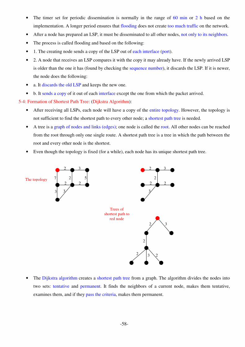
-58-

• The timer set for periodic dissemination is normally in the range of 60 min or 2 h based on the

implementation. A longer period ensures that flooding does not create too much traffic on the network.

• After a node has prepared an LSP, it must be disseminated to all other nodes, not only to its neighbors.

• The process is called flooding and based on the following:

• 1. The creating node sends a copy of the LSP out of each interface (port).

• 2. A node that receives an LSP compares it with the copy it may already have. If the newly arrived LSP

is older than the one it has (found by checking the sequence number), it discards the LSP. If it is newer,

the node does the following:

• a. It discards the old LSP and keeps the new one.

• b. It sends a copy of it out of each interface except the one from which the packet arrived.

5-4: Formation of Shortest Path Tree: (Dijkstra Algorithm):

• After receiving all LSPs, each node will have a copy of the entire topology. However, the topology is

not sufficient to find the shortest path to every other node; a shortest path tree is needed.

• A tree is a graph of nodes and links (edges); one node is called the root. All other nodes can be reached

from the root through only one single route. A shortest path tree is a tree in which the path between the

root and every other node is the shortest.

• Even though the topology is fixed (for a while), each node has its unique shortest path tree.

• The Dijkstra algorithm creates a shortest path tree from a graph. The algorithm divides the nodes into

two sets: tentative and permanent. It finds the neighbors of a current node, makes them tentative,

examines them, and if they pass the criteria, makes them permanent.

2 3

7 2 5

2 2

3 3

2 3

2

2 2

3

2 3

2

2 2 3

The topology

Trees of

shortest path to

red node

-59-

• Example:

Start

Set root to local node and move it

to tentative list.

Tentative list

empty? End

Among nodes in tentative list,

move the one with the shortest

path to permanent list.

Add each unprocessed neighbor of last moved node to tentative

list if not already there. If neighbor is in the tentative list with

larger cumulative cost, replace it with new one.

Yes

No

-60-

2 3

7 2 5

2 2

3 3

The topology

B C

D E F

G

A

A

- Permanent List {}

- Tentative List {A(0)}

Chose A and move it:

- Permanent List {A(0)}

Add A neighbors:

- Tentative List {B(2), D(7)}

2

7

B

D

A 2 3

7 2

B C

D E

A

Chose B and move it:

- Permanent List {A(0), B(2)}

Add B neighbors:

- Tentative List {D(7), C(5), E(4)}

2 3

2

2 2

3

B C

D E F

G

A

Chose E and move it:

- Permanent List {A(0), B(2), E(4)}

Add E neighbors, update their existing costs:

- Tentative List {D(6), C(5), F(6), G(7)}

2 3

2

2 2

3

B C

D E F

G

A

Chose C and move it:

- Permanent List {A(0), B(2), E(4), C(5)}

Add C neighbors:

- Tentative List {D(6), F(6), G(7)}

2 3

2

2 2

3

B C

D E F

G

A

Chose D and move it:

- Permanent List {A(0), B(2), E(4), C(5), D(6)}

Add D neighbors:

- Tentative List {F(6), G(7)}

2 3

2

2 2

3

B C

D E F

G

A

Chose F and move it:

- Permanent List {A(0), B(2), E(4), C(5), D(6),

F(6)}

Add F neighbors:

- Tentative List {G(7)} 2 3

2

2 2

3

B C

D E F

G

A

Chose G and move it:

- Permanent List {A(0), B(2), E(4), C(5), D(6),

F(6), G(7)}

Add G neighbors:

- Tentative List { }

-61-

5-5 Calculation of Routing Table from Shortest Path Tree:

• Each node uses the shortest path tree protocol to construct its routing table. The routing table shows the cost

of reaching each node from the root. The next table shows the routing table for node A:

Node Cost Next Router

A 0 -

B 2 -

C 5 B

D 6 B

E 4 B

F 6 B

G 7 B

• Both distance vector routing and link state routing end up with the same routing table for node A.

5-6 OSPF:

• The Open Shortest Path First or OSPF protocol is an intradomain routing protocol based on link state

routing. Its domain is also an autonomous system.

5-6-1 Areas:

• To handle routing efficiently and in a timely manner, OSPF divides an autonomous system into areas.

• An area is a collection of networks, hosts, and routers all contained within an autonomous system.

• An autonomous system can be divided into many different areas. All networks inside an area must be

connected.

• Routers inside an area flood the area with routing information. At the border of an area, special routers

called area border routers summarize the information about the area and send it to other areas.

• Among the areas inside an autonomous system is a special area called the backbone area; all the areas

inside an autonomous system must be connected to the backbone. In other words, the backbone serves as a

primary area and the other areas as secondary areas.

• If, because of some problem, the connectivity between a backbone and an area is broken, a virtual link

between routers must be created by an administrator to allow continuity of the functions of the backbone as

the primary area.

• Each area has an area identification. The area identification of the backbone is zero.

-62-

5-6-2 Metric:

• The OSPF protocol allows the administrator to assign a cost, called the metric, to each route. The

metric can be based on a type of service (minimum delay, maximum throughput, and so on).

• As a matter of fact, a router can have multiple routing tables, each based on a different type of

service.

5-6-2 Types of links:

• In OSPF terminology, a connection is called a link. Four types of links have been defined: point-

to-point, transient, stub, and virtual.

• A point-to-point link connects two routers without any other host or router in between. In other

words, the purpose of the link (network) is just to connect the two routers. Graphically, the routers

are represented by nodes, and the link is represented by a bidirectional edge connecting the nodes.

• A transient link is a network with several routers attached to it. The data can enter through any of

the routers and leave through any router. In this case, each router has many neighbors.

Graphical representation

Net Net Net

Net

Net Net

Net

Net Net Net

Area 0: Backbone

Area 1

Area 2

Autonomous System

Area border router Area border router

Backbone

router Backbone

router

AS boundary

router

-63-

• In order to apply the Dijkstra algorithm, we may represent each router with a node, and associate

an edge between each pair of routers.

• This is neither efficient nor realistic. It is not efficient because each router needs to advertise the

neighborhood to four other routers, for a total of 20 advertisements. It is not realistic because there

is no single network (link) between each pair of routers; there is only one network that serves as a

crossroad between all five routers.

• To show that each router is connected to every other router through one single network, the

network itself is represented by a node. However, because a network is not a machine, it cannot

function as a router. One of the routers in the network takes this responsibility. It is assigned a dual

purpose; it is a true router and a designated router.

• Now each router has only one neighbor, the designated router (network). On the other hand, the

designated router (the network) has five neighbors. We see that the number of neighbor

announcements is reduced from 20 to 10.

• The link is represented as a bidirectional edge between the nodes. However, while there is a metric

from each node to the designated router, there is no metric from the designated router to any other

node. When a packet enters a network, we assign a cost; when a packet leaves the network to go to

the router, there is no charge.

• A stub link is a network that is connected to only one router. The data packets enter the network

through this single router and leave the network through this same router. This is a special case of

the transient network.

• We can show this situation using the router as a node and using the designated router for the

network. However, the link is only one-directional, from the router to the network.

Ethernet Link

Unrealistic graphical representation

Net

Realistic graphical representation

-64-

• When the link between two routers is broken, the administration may create a virtual link between

them, using a longer path that probably goes through several routers.

• Example:

5-7 Comparison between DV and LS:

Ethernet Link Net


Net1

Net2 Net3

Net4

Net5

T1 line

T3 line

Autonomous system

R1

R2

R3

R4

R5

R6

R1 Net1 Net2

R2

R3

R4

R5

Net3 R6 Net4

Net5

2 3

5

7

8

4

2

5

2 3

2


-65-

DV: LS:

- Works fine with in small networks (AS) - Works fine in large networks (AS)

- Easy configuration. - Harder configuration.

- Less scalable. - More scalable.

- Less stable. - Stable.

- Slow convergence. - Faster convergence.

- Poor metrics (hops). - Richer metrics (bandwidth, delay).

N1

N2

N3

N4

512 kbps

10 Mbps

10 Mbps

10 Mbps

N1

N2

N3

N4

512 kbps

10 Mbps

10 Mbps

10 Mbps

DV: (1 hop) LS: (better bandwidth)

-66-

6- Path Vector Routing

• DV and LS routing are both intradomain routing protocols. They can be used inside an

autonomous system, but not between autonomous systems.

• These two protocols are not suitable for interdomain routing mostly because of scalability. Both of

these routing protocols become intractable when the domain of operation becomes large.

• DV routing is subject to instability if there are more than a few loops in the domain of operation.

• LS routing needs a huge amount of resources to calculate routing tables. It also creates heavy

traffic because of flooding.

• Path vector (PV) routing proved to be useful for interdomain routing.

• In path vector routing, we assume that there is one node (the speaker node) in each autonomous

system that acts on behalf of the entire autonomous system.

• The speaker node in an AS creates a routing table and advertises it to speaker nodes in the

neighboring ASs.

• The idea is the same as for DV routing except that only speaker nodes in each AS can

communicate with each other. However, what is advertised is different.

• A speaker node advertises the path, not the metric of the nodes, in its autonomous system or other

autonomous systems.

6-1 Initialization:

• At the beginning, each speaker node can know only the reachability of nodes inside its

autonomous system.

LAN LAN

LAN LAN

LAN LAN

LAN

Autonomous system Autonomous system

R1 R2

Speaker nodes Speaker nodes

-67-

• The above figure shows the initial tables for each speaker node in a system made of four ASs.

• Node Al is the speaker node for ASl, Bl for AS2, Cl for AS3, and D1 for AS4.

• Each speaker node creates an initial table that shows its corresponding local nodes that are located

in the same AS and can be reached through it.

6-2 Sharing:

• Just as in DV routing, in path vector routing, a speaker in an autonomous system shares its table

with immediate neighbors. In the above figure, node Al shares its table with nodes Bl and Cl. Node

Cl shares its table with nodes Bl, and Al. Node Bl shares its table with Cl, D1, and Al. Node Dl

shares its table with Bl only.

6-3 Updating:

• When a speaker node receives a two-column table from a neighbor, it updates its own table by

adding the nodes that are not in its routing table and add its own autonomous system to their

corresponding path. After a while each speaker has a table and knows how to reach each node in

other ASs.

A1 A2

A5 A4

A3

C1

C2 C3

B1 B3

B2 B4

D1

D3 D2

D4

AS1 AS3

AS2 AS4

A1 table Dest Path

A1 AS1

A2 AS1

A3 AS1

A4 AS1

A5 AS1

B1 table Dest Path

B1 AS2

B2 AS2

B3 AS2

B4 AS2

C1 table Dest Path

C1 AS3

C2 AS3

C3 AS3

D1 table Dest Path

D1 AS4

D2 AS4

D3 AS4

D4 AS4

-68-

• According to the figure above , if router Al receives a packet for nodes A3, it knows that the path is

in AS1 (the packet is at home); but if it receives a packet for Dl, it knows that the packet should go

from ASl, to AS2, and then to AS3. The routing table shows the path completely.

6-4 Loop prevention:

• The instability of DV routing and the creation of loops can be avoided in path vector routing.

When a router receives a message, it checks to see if its autonomous system is in the path list to the

destination. If it is, looping is involved and the message is ignored.

6-5 Policy routing:

• Policy routing can be easily implemented through path vector routing. When a router receives a

message, it can check the path. If one of the autonomous systems listed in the path is against its

policy, it can ignore that path and that destination.

• It does not update its routing table with this path, and it does not send this message to its

neighbors.

A1 A2

A5 A4

A3

C1

C2 C3

B1 B3

B2 B4

D1

D3 D2

D4

AS1 AS3

AS2 AS4

A1 table Dest Path

A1 AS1

A2 AS1

A3 AS1

A4 AS1

A5 AS1

B1 AS1, AS2

B2 AS1, AS2

B3 AS1, AS2

C1 AS1, AS2, AS3

C2 AS1, AS2, AS3

C3 AS1, AS2, AS3

C1 AS1, AS3

C2 AS1, AS3

C3 AS1, AS3

D1 AS1, AS2, AS4

D2 AS1, AS2, AS4

D3 AS1, AS2, AS4

D4 AS1, AS2, AS4

-69-

6-6 Optimum path:

• What is the optimum path in PV routing? We are looking for a path to a destination that is the best

for the organization that runs the autonomous system.

• We definitely cannot include metrics in this routing because each autonomous system that is

included in the path may use a different criterion for the metric. One system may use, internally,

RIP, which defines hop count as the metric; another may use OSPF with minimum delay defined

as the metric.

• The optimum path is the path that fits the organization. In our previous figure, each autonomous

system may have more than one path to a destination. For example, a path from AS4 to AS1 can be

AS4-AS2-AS3-AS1, or it can be AS4-AS2-AS1.

• For the tables, we chose the one that had the smaller number of autonomous systems, but this is

not always the case. Other criteria, such as security, safety, and reliability, can also be applied.

6-7 BGP:

• Border Gateway Protocol (BGP) is an interdomain routing protocol using PV routing.

• As we said before, the Internet is divided into hierarchical domains called autonomous systems.

We can divide autonomous systems into three categories: stub, multihomed, and transit.

6-7-1 Stub AS:

• A stub AS has only one connection to another AS. The interdomain data traffic in a stub AS can be

either created or terminated in the AS. The hosts in the AS can send data traffic to other ASs. The

hosts in the AS can receive data coming from hosts in other ASs. Data traffic, however, cannot

pass through a stub AS. A stub AS is either a source or a sink.

• A good example of a stub AS is a small corporation or a small local ISP.

6-7-2 Multihomed AS:

• A multihomed AS has more than one connection to other ASs, but it is still only a source or sink

for data traffic. It can receive data traffic from more than one AS. It can send data traffic to more

than one AS, but there is no transient traffic. It does not allow data coming from one AS and going

to another AS to pass through.

• A good example of a multihomed AS is a large corporation that is connected to more than one

regional or national AS that does not allow transient traffic.

6-7-3 Transit AS:

• A transit AS is a multihomed AS that also allows transient traffic.

• Good examples of transit ASs are national and international ISPs (Internet backbones).

-70-

Transport Layer: UDP

I- Introduction:

• The data link layer is responsible for delivery of frames between two neighboring nodes over a

link. This is called node-to-node delivery.

• The network layer is responsible for delivery of datagrams between two hosts. This is called host-

to-host delivery.

• Communication on the Internet is not defined as the exchange of data between two nodes or

between two hosts. Real communication takes place between two processes (application

programs). We need process-to-process delivery.

• We need a mechanism to deliver data from one of the processes running on the source host to the

corresponding process running on the destination host.

• The transport layer is responsible for process-to-process delivery. Two processes communicate in a

client/server relationship.

1- Client/Server Paradigm:

• The most common way to achieve process-to-process delivery is the client/server paradigm. A

process on the local host, called a client, needs services from a process usually on the remote host,

called a server.

• Both processes (client and server) have the same name. For example, to get a web page from a

remote machine, we need an HTTP client process running on the local host and an HTTP server

process running on a remote machine.

• Operating systems today support both multiuser and multiprogramming environments.

• A remote computer can run several server programs at the same time, just as local computers can

run one or more client programs at the same time.

Processes Processes

Node-to-node Node-to-node Node-to-node Node-to-node Node-to-node

Host-to-host

Process-to-process

-71-

2- Addressing:

• Whenever we need to deliver something to one specific destination among many, we need an

address.

• At the data link layer, we need a MAC address to choose one node among several nodes if the

connection is not point-to-point.

• At the network layer, we need an IP address to choose one host among millions.

• At the transport layer, we need a transport layer address, called a port number, to choose among

multiple processes running on the destination host.

• In the Internet model, the port numbers are 16-bit integers between 0 and 65,535.

• The client program defines itself with a port number, chosen randomly by the transport layer

software running on the client host. This is the ephemeral port number.

• The server process must also define itself with a port number. This port number, however, cannot

be chosen randomly.

• The Internet has decided to use universal port numbers for servers; these are called well-known

port numbers.

• There are some exceptions to this rule; for example, there are clients that are assigned well-known

port numbers. Every client process knows the well-known port number of the corresponding server

process. For example, while the HTTP client process, discussed above, can use an ephemeral

(temporary) port number 52,000 to identify itself, the HTTP server process must use the well-

known (permanent) port number 80.

3- IANA Ranges:

• The IANA (Internet Assigned Number Authority) has divided the port numbers into three ranges:

well known, registered, and dynamic (or private).

• 1- Well-known ports: The ports ranging from 0 to 1023 are assigned and controlled by IANA.

Processes

HTTP

client

Processes

HTTP

server

Data 52,000 80

Data 52,000 80

Source

Port

Destin.

Port

-72-

• 2- Registered ports: The ports ranging from 1024 to 49,151 are not assigned or controlled by

IANA. They can only be registered (on demand) with IANA to prevent duplication.

• 3- Dynamic ports: The ports ranging from 49,152 to 65,535 are neither controlled nor registered.

They can be used by any process. These are the ephemeral ports.

4- Connectionless Versus Connection-Oriented Service

• A transport layer protocol can either be connectionless or connection-oriented.

• In a connectionless service, the packets are sent from one party to another with no need for

connection establishment or connection release. The packets may be delayed or lost or may arrive

out of sequence. There is no acknowledgment either.

• UDP, is connectionless.

• In a connection-oriented service, a connection is first established between the sender and the

receiver. Data are transferred in order. At the end, the connection is released.

• TCP and SCTP are connection-oriented protocols.

5- Reliable Versus Unreliable:

• The transport layer service can be reliable or unreliable.

• If the application layer program needs reliability, we use a reliable transport layer protocol by

implementing flow and error control at the transport layer. This means a slower and more complex

service.

• On the other hand, if the application program does not need reliability because it uses its own flow

and error control mechanism or it needs fast service or the nature of the service does not demand

flow and error control (real-time applications), then an unreliable protocol can be used.

• In the Internet, there are three common different transport layer protocols: UDP is connectionless

and unreliable; TCP and SCTP are connection oriented and reliable.

• Why do we need error and flow control in the transport layer if the data link layer is reliable and

has flow and error control? The answer is because the network layer in the Internet is unreliable

(best-effort delivery).

-73-

6- Three Protocols:

• The original TCP/IP protocol suite specifies two protocols for the transport layer: UDP and TCP. A

new transport layer protocol, SCTP, has been designed.

II- USER DATAGRAM PROTOCOL (UDP):

• The User Datagram Protocol (UDP) is called a connectionless, unreliable transport protocol. It

performs very limited error checking.

• UDP is a very simple protocol using a minimum of overhead. If a process wants to send a small

message and does not care much about reliability, it can use UDP. Sending a small message by using

UDP takes much less interaction between the sender and receiver than using TCP or SCTP.

IGMP ICMP

ARP RARP

IP Network

Layer

Data Link

Layer

Physical

Layer

Ethernet (802.3), Token Ring (802.5),

Token Bus (802.4), Wireless (802.11), …

UDP TCP SCTP Transport

Layer

Application

Layer BootP Echo HTTP SMTP …….

Transport

Network

Data Link

Physical

Error checked by data link layer

Error not checked by data link layer

-74-

1- Well-Known Ports for UDP:

• The next table shows some well-known port numbers used by UDP. Some port numbers can be used

by both UDP and TCP.

Port Protocol Description

7 Echo Echoes a received datagram back to the sender

11 Users Active users

13 Daytime Returns the date and the time

53 Nameserver Domain Name Service

67 Bootps Server port to download bootstrap information

68 Bootpc Client port to download bootstrap information

69 TFTP Trivial File Transfer Protocol

123 NTP Network time protocol

• In LUNIX operating systems, the well-known ports are stored in a file called /etc/services. Each line in

this file gives the name of the server and the well-known port number. We can use the grep utility to

extract the line corresponding to the desired application. The following shows the port for FTP and

HTTP. Note that FTP (or HTTP) can use port 21 (or 80) with either UDP, TCP or SCTP.

$grep ftp /etc/services

ftp 21/tcp

ftp 21/udp

ftp 21/sctp

…

$grep http /etc/services

http 80/tcp

http 80/udp

…

$grep sctp /etc/services

ftp 21/sctp

ssh 22/sctp

…

-75-

2- User Datagram

• UDP packets, called user datagrams, have a fixed-size header of 8 bytes.

• Source port number: This is the port number used by the process running on the source host. It is 16

bits long, which means that the port number can range from 0 to 65,535. If the source host is the client

(a client sending a request), the port number, in most cases, is an ephemeral port number requested by

the process and chosen by the UDP software running on the source host. If the source host is the server

(a server sending a response), the port number, in most cases, is a well-known port number.

• Destination port number: This is the port number used by the process running on the destination host. It

is also 16 bits long. If the destination host is the server (a client sending a request), the port number, in

most cases, is a well-known port number. If the destination host is the client (a server sending a

response), the port number, in most cases, is an ephemeral port number. In this case, the server copies

the ephemeral port number it has received in the request packet.

• Length: This is a 16-bit field that defines the total length of the user datagram, header plus data. The 16

bits can define a total length of 0 to 65,535 bytes. However, the total length needs to be much less

because a UDP user datagram is encapsulated in an IP datagram with a total length of 65,535 bytes.

• The length field in a UDP user datagram is actually not necessary because there is a field in the IP

datagram that defines the total length and another field in the IP datagram that defines the length of the

header (of IP datagram). So if we subtract the header length from the total length, we can deduce the

length of a UDP datagram that is encapsulated in an IP datagram.

• However, the designers of the UDP protocol felt that it was more efficient for the destination UDP to

calculate the length of the data from the information provided in the UDP user datagram rather than ask

the IP software to supply this information.

• Checksum: This field is used to detect errors over the entire user datagram (header plus data).

3- UDP Operation:

1- Connectionless Services:

• UDP provides a connectionless service. This means that each user datagram sent by UDP is an

independent datagram. There is no relationship between the different user datagrams even if they

are coming from the same source process and going to the same destination program.

Header Data (from application layer)

Source port number

16 bits

8 bytes

Destination port number

16 bits

Total length

16 bits

Checksum

16 bits

-76-

• The user datagrams are not numbered.

• Also, there is no connection establishment and no connection termination, as is the case for TCP.

This means that each user datagram can travel on a different path.

• One of the ramifications (disadvantages) of being connectionless is that the process that uses UDP

cannot send a stream of data to UDP and expect UDP to chop them into different related user

datagrams. Instead each request must be small enough to fit into one user datagram. Only those

processes sending short messages should use UDP.

2- Flow and Error Control:

• UDP is a very simple, unreliable transport protocol. There is no flow control and hence no window

mechanism. The receiver may overflow with incoming messages.

• There is no error control mechanism in UDP except for the checksum. This means that the sender

does not know if a message has been lost or duplicated. When the receiver detects an error through

the checksum, the user datagram is silently discarded.

• The lack of flow control and error control means that the process using UDP should provide these

mechanisms.

3- Encapsulation and Decapsulation

• To send a message from one process to another, the UDP protocol encapsulates and decapsulates

messages in an IP datagram.

4- Use of UDP:

• UDP is suitable for a process that requires simple request-response communication with little

concern for flow and error control. It is not usually used for a process such as ftp that needs to send

bulk data.

• UDP is suitable for a process with internal flow and error control mechanisms. For example, the

Trivial File Transfer Protocol (TFTP) process includes flow and error control. It can easily use

UDP.

• UDP is a suitable transport protocol for multicasting. Multicasting capability is embedded in the

UDP software but not in the TCP software.

• UDP is used for management processes such as SNMP.

• UDP is used for some route updating protocols such as Routing Information Protocol (RIP).

Header Data

Header Data

UDP datagram

IP datagram

-77-

Transport Layer: TCP

I- Introduction:

• The second transport layer is called Transmission Control Protocol (TCP).

• TCP, like UDP, is a process-to-process (program-to-program) protocol. TCP, therefore, like UDP,

uses port numbers.

• Unlike UDP, TCP is a connection oriented protocol; it creates a virtual connection between two

TCPs to send data.

• In addition, TCP is reliable; it uses flow and error control mechanisms at the transport level.

II- TCP Services:

1- Process-to-Process Communication:

• Like UDP, TCP provides process-to-process communication using port numbers. The next table

lists some well-known port numbers used by TCP:

Port Protocol Description

7 Echo Echoes a received datagram back to the sender

11 Users Active users

13 Daytime Returns the date and the time

20 FTP (data) File Transfer Protocol (data connection)

21 FTP (control) File Transfer Protocol (control connection)

53 DNS Domain Name Service

67 Bootp port to download bootstrap information

80 HTTP Hypertext Transfer Protocol

2- Stream Delivery Service:

• TCP, unlike UDP, is a stream-oriented protocol. In UDP, each message is called a user datagram

and becomes, eventually, one IP datagram. Neither IP nor UDP recognizes any relationship

between the datagrams.

• TCP, on the other hand, allows the sending process to deliver data as a stream of bytes (not

segments) and allows the receiving process to obtain data as a stream of bytes. TCP creates an

environment in which the two processes seem to be connected by an imaginary "tube" that carries

their data across the Internet.

-78-

2-1 Buffering:

• Because the sending and the receiving processes may not write or read data at the same speed, TCP

needs buffers for storage. There are two buffers, the sending buffer and the receiving buffer, one for

each direction. These buffers are also necessary for flow and error control mechanisms used by TCP.

2-2 Segments:

• The IP layer, as a service provider for TCP, needs to send data in packets, not as a stream of bytes. At

the transport layer, TCP groups a number of bytes together into a packet called a segment.

• TCP adds a header to each segment (for control purposes) and delivers the segment to the IP layer for

transmission. The segments are encapsulated in IP datagrams and transmitted.

• This entire operation is transparent (not aware) to the receiving process. The segments may be received

out of order, lost, or corrupted and resent. All these are handled by TCP with the receiving process

unaware of any activities.

3- Full-Duplex Communication:

• TCP offers full-duplex service, in which data can flow in both directions at the same time. Each TCP

connection then has a sending and receiving buffer, and segments move in both directions.

4- Connection-Oriented Service:

• TCP, unlike UDP, is a connection-oriented protocol. When a process at site A wants to send and

receive data from another process at site B, the following occurs:

1. The two TCPs establish a connection between them.

2. Data are exchanged in both directions.

3. The connection is terminated.

• Note that this is a virtual connection, not a physical connection. The TCP segment is encapsulated in an

IP datagram and can be sent out of order, or lost, or corrupted, and then resent. Each may use a

different path to reach the destination.

• TCP creates a stream-oriented environment in which it accepts the responsibility of delivering the

bytes in order to the other site.

5- Reliable Service:

• TCP is a reliable transport protocol. It uses an acknowledgment mechanism to check the safe and

sound arrival of data.

TCP

Sending Process

TCP

Receiving Process

Virtual Connection

Stream of bytes

-79-

III- TCP Features:

• To provide the services mentioned in the previous section, TCP has several features that are discussed

next.

1- Numbering System:

• Although the TCP software keeps track of the segments being transmitted or received, there is no field

for a segment number value in the segment header. Instead, there are two fields called the sequence

number and the acknowledgment number.

1-1 Byte Number:

• TCP numbers all data bytes that are transmitted in a connection. Numbering is independent in each

direction.

• The numbering does not necessarily start from 0. Instead, TCP generates a random number between 0

and 232 - 1 for the number of the first byte. For example, if the random number happens to be 1057 and

the total data to be sent are 6000 bytes, the bytes are numbered from 1057 to 7056. The byte numbering

is used for flow and error control.

1-2 Sequence Number:

• After the bytes have been numbered, TCP assigns a sequence number to each segment that is being

sent. The sequence number for each segment is the number of the first byte carried in that segment.

• Example: Suppose a TCP connection is transferring a file of 5000 bytes. The first byte is numbered

10,00l. What are the sequence numbers for each segment if data are sent in five segments, each

carrying 1000 bytes?

Segment 1 Sequence Number: 10,001 (range: 10,001 to 11,000)





2-3 Acknowledgment Number:

• Each party (sender or receiver) uses an acknowledgment number to confirm the bytes it has received.

• The acknowledgment number defines the number of the next byte that the party expects to receive.

• The acknowledgment number is cumulative, which means that the party takes the number of the last

byte that it has received, safe and sound, adds 1 to it, and announces this sum as the acknowledgment

number.

• Example: if a party uses 5643 as an acknowledgment number, it has received all bytes from the

beginning up to 5642. Note that this does not mean that the party has received 5642 bytes because the

first byte number does not have to start from 0.

-80-

2- Flow Control:

• TCP, unlike UDP, provides flow control. The receiver of the data controls the amount of data that

are to be sent by the sender. This is done to prevent the receiver from being overwhelmed with

data. The numbering system allows TCP to use a byte-oriented (not segment-oriented) flow

control.

3- Error Control:

• To provide reliable service, TCP implements an error control mechanism. Although error control

considers a segment as the unit of data for error detection (loss or corrupted segments), error

control is byte-oriented.

4- Congestion Control:

• TCP, unlike UDP, takes into account congestion in the network. The amount of data sent by a

sender is not only controlled by the receiver (flow control), but is also determined by the level of

congestion in the network.

IV- Segment:

• The segment consists of a 20- to 60-byte header, followed by data from the application program.

The header is 20 bytes if there are no options and up to 60 bytes if it contains options.

1- Format:

• The format of a segment is shown as follows:

• Source port address: This is a 16-bit field that defines the port number of the application program

in the host that is sending the segment. This serves the same purpose as the source port address in

the UDP header.

Header Data

Source Port Address

16 bits

Destination Port Address

16 bits

Sequence Number

32 bits

Acknowledgement Number

32 bits

Window Size

16 bits

HLEN

4 bits

Reserved

6 bits

Control

6 bits

Checksum

16 bits

Urgent Pointer

16 bits

Option and Padding

32 bits

-81-

• Destination port address: This is a 16-bit field that defines the port number of the application

program in the host that is receiving the segment. This serves the same purpose as the destination

port address in the UDP header.

• Sequence number: This 32-bit field defines the number assigned to the first byte of data contained

in this segment.

• Acknowledgment number: This 32-bit field defines the byte number that the receiver of the

segment is expecting to receive from the other party. If the receiver of the segment has

successfully received byte number x from the other party, it defines x + 1 as the acknowledgment

number. Acknowledgment and data can be piggybacked together.

• Header length: This 4-bit field indicates the number of 4-byte words in the TCP header. The length

of the header can be between 20 and 60 bytes. Therefore, the value of this field can be between 5

(5 x 4 =20) and 15 (15 x 4 =60).

• Reserved: This is a 6-bit field reserved for future use.

• Control: This field defines 6 different control bits or flags. These bits enable flow control,

connection establishment and termination, connection abortion, and the mode of data transfer in

TCP.

Flag Description

URG (bit # 1) The value of the urgent pointer field is valid

ACK (bit # 2) The value of the acknowledgement field is valid

PSH (bit # 3) Push the data

RST (bit # 4) Reset the connection

SYN (bit # 5) Synchronize sequence numbers during connection

FIN (bit # 6) Terminate the connection

• Window size: This field defines the size of the window, in bytes, that the other party must

maintain. Note that the length of this field is 16 bits, which means that the maximum size of the

window is 65,535 bytes. This value is normally referred to as the receiving window (rwnd) and is

determined by the receiver. The sender must obey the dictation of the receiver in this case.

• Checksum: This 16-bit field contains the checksum. The calculation of the checksum for TCP

follows the same procedure as the one described for UDP (header + data). However, the inclusion

of the checksum in the UDP datagram is optional, whereas the inclusion of the checksum for TCP

is mandatory. In addition, the only action taken in UDP in case of an error is discarding the

datagram while in TCP an error control mechanism is launched.

-82-

• Urgent pointer: This l6-bit field, which is valid only if the urgent flag is set, is used when the

segment contains urgent data. It defines the number that must be added to the sequence number to

obtain the number of the last urgent byte in the data section of the segment.

• Options: There can be up to 40 bytes of optional information in the TCP header.

V- A TCP Connection:

• TCP is connection-oriented. A connection-oriented transport protocol establishes a virtual path

between the source and destination. All the segments belonging to a message are then sent over

this virtual path. Using a single virtual pathway for the entire message facilitates the

acknowledgment process as well as retransmission of damaged or lost frames.

• How TCP, which uses the services of IP, a connectionless protocol, can be connection-oriented.

The point is that a TCP connection is virtual, not physical. TCP operates at a higher level. TCP

uses the services of IP to deliver individual segments to the receiver, but it controls the connection

itself. If a segment is lost or corrupted, it is retransmitted.

• Unlike TCP, IP is unaware of this retransmission. If a segment arrives out of order, TCP holds it

until the missing segments arrive; IP is unaware of this reordering.

• In TCP, connection-oriented transmission requires three phases: connection establishment, data

transfer, and connection termination.

1- Connection Establishment:

• TCP transmits data in full-duplex mode. When two TCPs in two machines are connected, they are

able to send segments to each other simultaneously. This implies that each party must initialize

communication and get approval from the other party before any data are transferred.

• The connection establishment in TCP is called three way handshaking. In our example, an

application program, called the client, wants to make a connection with another application

program, called the server, using TCP as the transport layer protocol.

• The process starts with the server. The server program tells its TCP that it is ready to accept a

connection. This is called a request for a passive open. Although the server TCP is ready to accept

any connection from any machine in the world, it cannot make the connection itself.

• The client program issues a request for an active open. A client that wishes to connect to an open

server tells its TCP that it needs to be connected to that particular server. TCP can now start the

three-way handshaking process as shown next.

-83-

• Step 1: The client sends the first segment, a SYN segment, in which only the SYN flag is set. This

segment is for synchronization of sequence numbers. It consumes one sequence number. When the

data transfer starts, the sequence number is incremented by 1. We can say that the SYN segment

carries no real data, but we can think of it as containing 1 imaginary byte.

• Step 2: The server sends the second segment, a SYN +ACK segment, with 2 flag bits set: SYN and

ACK. This segment has a dual purpose. It is a SYN segment for communication in the other

direction and serves as the acknowledgment for the received SYN segment. It consumes one

sequence number.

• Step 3: The client sends the third segment. This is just an ACK segment. It acknowledges the

receipt of the second segment with the ACK flag and acknowledgment number field. Note that the

sequence number in this segment is the same as the one in the SYN segment; the ACK segment

does not consume any sequence numbers.

• SYN Flooding Attack: The connection establishment procedure in TCP is susceptible to a serious

security problem called the SYN flooding attack. This happens when a malicious attacker sends a

large number of SYN segments to a server, pretending that each of them is corning from a

different client by faking the source IP addresses in the datagrams.

• The server, assuming that the clients are issuing an active open, allocates the necessary resources,

such as creating communication tables and setting timers. The TCP server then sends the SYN

+ACK segments to the fake clients, which are lost. During this time, however, a lot of resources

are occupied without being used. If, during this short time, the number of SYN segments is large,

the server eventually runs out of resources and may crash. This SYN flooding attack belongs to a

type of security attack known as a denial-of-service attack, in which an attacker monopolizes a

system with so many service requests that the system collapses and denies service to every request.

Client Server

Seq. num: 8000

Ack. num: ?

ACK flag: 0

SYN flag: 1

Seq. num: 15000

Ack. num: 8001

ACK flag: 1

SYN flag: 1

Seq. num: 8000

Ack. num: 15001

ACK flag: 1

SYN flag: 0

SYN

segment

SYN + ACK

segment

ACK

segment

Active open Passive open

-84-

2- Data Transfer

• After connection is established, bidirectional data transfer can take place. The client and server can

both send data and acknowledgments. We will study the rules of

• The acknowledgment is piggybacked with the data.

• In the example above, after connection is established (not shown in the figure), the client sends

2000 bytes of data in two segments. The server then sends 2000 bytes in one segment.

• The client sends one more segment. The first three segments carry both data and acknowledgment,

but the last segment carries only an acknowledgment because there are no more data to be sent.

Note the values of the sequence and acknowledgment numbers. The data segments sent by the

client have the PSH (push) flag set so that the server TCP knows to deliver data to the server

process as soon as they are received.

• The segment from the server, on the other hand, does not set the push flag. Most TCP

implementations have the option to set or not set this flag.

• Pushing Data: We saw that the sending TCP uses a buffer to store the stream of data coming from

the sending application program. The sending TCP can select the segment size. The receiving TCP

also buffers the data when they arrive and delivers them to the application program when the

Client Server

Seq. num: 8001

Ack. num: 15001

ACK flag: 1

PSH flag: 1 Data

segment

Data: 8001 - 9000

Seq. num: 9001

Ack. num: 15001

ACK flag: 1

PSH flag: 1 Data

segment

Data: 9001 - 10000

Seq. num: 15001

Ack. num: 10001

ACK flag: 1

PSH flag: 0 Data

segment

Data: 15001 - 17000

Seq. num: 10000

Ack. num: 17001

ACK flag: 1

PSH flag: 0

Window size: 10000

ACK

segment

-85-

application program is ready or when it is convenient for the receiving TCP. This type of

flexibility increases the efficiency of TCP.

• However, on occasion the application program has no need for this flexibility. For example,

consider an application program that communicates interactively with another application program

on the other end. The application program on one site wants to send a keystroke to the application

at the other site and receive an immediate response. Delayed transmission and delayed delivery of

data may not be acceptable by the application program.

• TCP can handle such a situation. The application program at the sending site can request a push

operation. This means that the sending TCP must not wait for the window to be filled. It must

create a segment and send it immediately. The sending TCP must also set the push bit (PSH) to let

the receiving TCP know that the segment includes data that must be delivered to the receiving

application program as soon as possible and not to wait for more data to come.

• Urgent Data: On occasion an application program needs to send urgent bytes. This means that the

sending application program wants a piece of data to be read out of order by the receiving

application program. As an example, suppose that the sending application program is sending data

to be processed by the receiving application program. When the result of processing comes back,

the sending application program finds that everything is wrong. It wants to abort the process, but it

has already sent a huge amount of data. If it issues an abort command (control +C), these two

characters will be stored at the end of the receiving TCP buffer. It will be delivered to the receiving

application program after all the data have been processed.

• The solution is to send a segment with the URG bit set. The sending application program tells the

sending TCP that the piece of data is urgent. The sending TCP creates a segment and inserts the

urgent data at the beginning of the segment. The rest of the segment can contain normal data from

the buffer. The urgent pointer field in the header defines the end of the urgent data and the start of

normal data.

• When the receiving TCP receives a segment with the URG bit set, it extracts the urgent data from

the segment, using the value of the urgent pointer, and delivers them, out of order, to the receiving

application program.

3- Connection Termination:

• Any of the two parties involved in exchanging data (client or server) can close the connection,

although it is usually initiated by the client.

• Most implementations today allow two options for connection termination: three-way handshaking

and four-way handshaking with a half-close option.

-86-

3-1 Three-Way Handshaking:

• Step 1: In a normal situation, the client TCP, after receiving a close command from the client

process, sends the first segment, a FIN segment in which the FIN flag is set.

• Note that a FIN segment can include the last chunk of data sent by the client, or it can be just a

control segment. If it is only a control segment, it consumes only one sequence number.

• Step 2: The server TCP, after receiving the FIN segment, informs its process of the situation and

sends the second segment, a FIN +ACK segment, to confirm the receipt of the FIN segment from

the client and at the same time to announce the closing of the connection in the other direction.

This segment can also contain the last chunk of data from the server. If it does not carry data, it

consumes only one sequence number.

• Step 3: The client TCP sends the last segment, an ACK segment, to confirm the receipt of the FIN

segment from the TCP server. This segment contains the acknowledgment number, which is 1 plus

the sequence number received in the FIN segment from the server. This segment cannot carry data

and consumes no sequence numbers.

3-2 Half-Close :

• In TCP, one end can stop sending data while still receiving data. This is called a half-close.

Although either end can issue a half-close, it is normally initiated by the client. It can occur when

the server needs all the data before processing can begin.

• A good example is sorting. When the client sends data to the server to be sorted, the server needs

to receive all the data before sorting can start. This means the client, after sending all the data, can

close the connection in the outbound direction. However, the inbound direction must remain open

to receive the sorted data.

• The server, after receiving the data, still needs time for sorting; its outbound direction must remain

open.

Client Server

Seq. num: x

Ack. num: y

ACK flag: 0

FIN flag: 1

Seq. num: y

Ack. num: x + 1

ACK flag: 1

FIN flag: 1

Seq. num: x

Ack. num: y + 1

ACK flag: 1

SYN flag: 0

FIN

segment

FIN + ACK

segment

ACK

segment

Active close Passive close

-87-

• Step 1: The client half-closes the connection by sending a FIN segment.

• Step2: The server accepts the half-close by sending the ACK segment.

• Step 3: The data transfer from the client to the server stops. The server, however, can still send

data. When the server has sent all the processed data, it sends a FIN segment, which is

acknowledged (Step 4) by an ACK from the client.

• After half-closing of the connection, data can travel from the server to the client and

acknowledgments can travel from the client to the server. The client cannot send any more data to

the server.

• Note the sequence numbers we have used. The second segment (ACK) consumes no sequence

number. Although the client has received sequence number y - 1 and is expecting y, the server

sequence number is still y - 1.

• When the connection finally closes, the sequence number of the last ACK segment is still x,

because no sequence numbers are consumed during transmission in that direction.

Client Server

Seq. num: x

Ack. num: y

ACK flag: 0

FIN flag: 1

Seq. num: y - 1

Ack. num: x + 1

ACK flag: 1

FIN flag: 0

Seq. num: x

Ack. num: z + 1

ACK flag: 1

SYN flag: 0

FIN

segment

ACK segment

ACK

segment

Active close

Passive close

Data segments

from server to client

Acknowledged segments

from client to server

Seq. num: x

Seq. num: z

Ack. num: x + 1

ACK flag: 1

FIN flag: 1 FIN + ACK

segment

-88-

3- Flow Control

• TCP uses a sliding window to handle flow control.

• The sliding window protocol used by TCP, however, is something between the Go-Back-N and

Selective Repeat sliding window.

• The sliding window protocol in TCP looks like the Go-Back-N protocol because it does not use

NAKs.

• It looks like Selective Repeat because the receiver holds the out-of-order segments until the

missing ones arrive.

• There are two big differences between this sliding window and the one we used at the data link

layer. First, the sliding window of TCP is byte-oriented; the one we discussed in the data link layer

is frame-oriented. Second, the TCP's sliding window is of variable size; the one we discussed in

the data link layer was of fixed size.

• The sender window is always less than or equal to the receiver window.

• The window spans a portion of the buffer containing bytes received from the process. The bytes

inside the window are the bytes that can be in transit; they can be sent without worrying about

acknowledgment.

211 210 209 208 207 206 205 204 203

At the sender:

Next byte to be sent

Size = receiver window

211 210 209 208 207 206 205 204 203

Bytes not

sent yet

Bytes ready to

be immediately

sent

Bytes already

sent but not

acknowledged

Bytes sent and

acknowledged

At the sender:

-89-

3-1 Deciding the receiver window:

• The receiver window is variable. It depends on two factors: the size of the buffer and the processed

bytes:

• Receiver window size = buffer size – unprocessed data.

• Example: What is the value of the receiver window (rwnd) for host A if the receiver, host B, has a

buffer size of 5000 bytes and 1000 bytes of received and unprocessed data?

• Solution: The value of rwnd =5000 - 1000 = 4000. Host B can receive only 4000 bytes of data

before overflowing its buffer. Host B advertises this value in its next segment to A.

3-2 Deciding the sender window:

• We know that the sender's window is always lesser than the receiver window. Yet, another factor

must be taken in consideration: congestion. The sender can get information about congestion in the

network and decide its window size.

• Sender window size = minimum (receiver window size, congestion window size).

3-3 Sliding the sender window:

• Once the receiver verifies the integrity of the received bytes, it sends an acknowledgement (could

be piggybacked) to the sender with the number of the expected byte.

3-4 Expanding the sender window:

• If the receiver process consumes data faster than it receives, the size of the receiver window

expands.

• In this case, the receiver updates the window size field in the TCP header with the new size and

sends it to the sender in the next TCP segment.

211 210 209 208 207 206 205

At the sender:


212

211 210 209 208 207 206 205

At the sender:


After receiving ACK expecting byte 205

-90-

3-5 Shrinking the sender window:

• If the receiver process consumes data slower than it receives, the size of the receiver window

shrinks.

• In this case, the receiver updates the window size field in the TCP header with the new size and

sends it to the sender in the next TCP segment.

• Shrinking is not recommended since some bytes can be revoked from being acknowledged:

3-2 Closing the sender window:

• If the buffer of the receiver is full, it sets the window size to be zero and informs the sender. In this

case the sender recess sending bytes until receiving a non-zero window size.

4- Error Control:

• TCP is reliable: it handles error control using timers, acknowledgements and retransmissions.

• TCP has no negative acknowledgement.

• There are three cases

4-1 Lost or corrupted segment and lost acknowledgment:

• Once the receiver checks the integrity of a segment and finds it corrupted, it simply discards it.

• The sender sets a timer for each segment. If an acknowledgement is received for this segment or

for any of its successors than the timer is destroyed and the segment is considered safe.

• If the timer goes off before receiving an acknowledgement, the sender consider that the segment

was lost or corrupted. In this case, it retransmits the segment and sets its timer.

• On the other hand, if an acknowledgement is lost, then the sender's timer goes off and the

corresponding segment is retransmitted.

4-2 Duplicate segment and acknowledgement:

• If an acknowledgement for a segment is delayed and arrived after retransmitting the segment, the

sender consider it as the real acknowledgment, and ignore any other duplicates.

• In this case, the receiver also might receive a duplicate segment of bytes. Then, by checking the

sequence number of the segment, it knows that it has been already acknowledged, so it simply

discards it.

211 210 209 208 207 206 205

At the sender:


212

This byte is revoked

-91-

4-3 Out-of-order segments:

• TCP used an unreliable IP service that guarantees no order of the transmitted datagrams.

• TCP handles this problem by delaying the acknowledgement of a segment until receiving its

predecessors.

-92-

Transport Layer: Congestion Control

I - DATA TRAFFIC:

• The main focus of congestion control and quality of service is data traffic.

• In congestion control we try to avoid traffic congestion.

• In quality of service, we try to create an appropriate environment for the traffic.

1- Traffic Descriptor:

• Traffic descriptors are qualitative values that represent a data flow.

1-1 Average Data Rate:

• The average data rate is the number of bits sent during a period of time, divided by the number of

seconds in that period. Average data rate = Amount of data / Time

• The average data rate is a very useful characteristic of traffic because it indicates the average

bandwidth needed by the traffic.

1-2 Peak Data Rate:

• The peak data rate defines the maximum data rate of the traffic.

• The peak data rate is a very important measurement because it indicates the peak bandwidth that

the network needs for traffic to pass through.

1-3 Maximum Burst Size:

• Although the peak data rate is a critical value for the network, it can usually be ignored if the

duration of the peak value is very short.

• Example: if data are flowing steadily at the rate of 1 Mbps with a sudden peak data rate of 2 Mbps

for just 1 ms, the network probably can handle the situation. However, if the peak data rate lasts 60

ms, there may be a problem for the network.

• The maximum burst size normally refers to the maximum length of time the traffic is generated at

the peak rate.

Time

Data rate

Average data rate Maximum data rate

Maximum

Burst size

-93-

1-4 Effective Bandwidth:

• The effective bandwidth is the bandwidth that the network needs to allocate for the flow of traffic.

The effective bandwidth is a function of three values:

• Effective bandwidth = F(average data rate, peak data rate, maximum burst size).

• The calculation of this value is very complex. Yet, in case of very small maximum burst size, this

value depends only on average data rate. Thus, the calculation is based on Shannon and Nyquist

theories.

2- Traffic Profiles:

• A data flow can have one of the following traffic profiles (types): constant bit rate, variable bit

rate, or bursty.

2-1 Constant Bit Rate:

• A constant-bit-rate (CBR) traffic model has a data rate that does not change (not realistic).

• In this type of flow, the average data rate and the peak data rate are the same.

• The maximum burst size is not applicable (infinite). This type of traffic is very easy for a network

to handle since it is predictable. The network knows in advance how much bandwidth to allocate

for this type of flow.

• An analogy to constant traffic is the water flow on a fleet (SAGUIA).

2-2 Variable Bit Rate:

• In the variable-bit-rate (VBR) category, the rate of the data flow changes in time, with the changes

smooth instead of sudden and sharp.

• In this type of flow, the average data rate and the peak data rate are different. The maximum burst

size is usually a small value.

• This type of traffic is more difficult to handle than constant-bit-rate traffic, but it normally does not

need to be reshaped (we will see it in quality of service).

• An analogy to variable traffic is the car traffic during regular hours.

Time

Data rate

-94-

2-3 Bursty:

• In the bursty data category, the data rate changes suddenly in a very short time. It may jump from

zero, for example, to 1 Mbps in a few microseconds and vice versa. It may also remain at this

value for a while.

• The average bit rate and the peak bit rate are very different values in this type of flow. The

maximum burst size is significant. This is the most difficult type of traffic for a network to handle

because the profile is very unpredictable. To handle this type of traffic, the network normally

needs to reshape it, using reshaping techniques.

• Bursty traffic is one of the main causes of congestion in a network.

• An analogy to bursty traffic is the car traffic during rush hours.

II- CONGESTION:

• An important issue in a packet-switched network is congestion.

• Congestion in a network may occur if the load on the network (the number of packets sent to the

network) is greater than the capacity of the network (the number of packets a network can handle).

• Congestion control refers to the mechanisms and techniques to control the congestion and keep the

load below the capacity.

• Congestion in a network or internetwork occurs because routers and switches have queues or

buffers that hold the packets before and after processing.

• A router has an input queue and an output queue for each interface. When a packet arrives at the

incoming interface, it undergoes three steps before departing:

1. The packet is put at the end of the input queue while waiting to be checked.

Time

Data rate

Time

Data rate

-95-

2. The processing module of the router removes the packet from the input queue once it reaches

the front of the queue and uses its routing table and the destination address to find the route.

3. The packet is put in the appropriate output queue and waits its turn to be sent.

• Practically, there will be no congestion if each packet is processed faster than it waits in the input

queue, and if it is sent faster than it waits in the output queue.

1 - Network Performance:

• Congestion control involves two factors that measure the performance of a network: delay and

throughput.

1-1 Delay Versus Load:

• When the load is much less than the capacity of the network, the delay is at a minimum. This

minimum delay is composed of propagation delay (in wires) and processing delay (in switches or

routers), both of which are negligible.

• However, when the load reaches the network capacity, the delay increases sharply because we now

need to add the waiting time in the queues (for all routers in the path) to the total delay.

• Note that the delay becomes infinite when the load is greater than the capacity. Consider the size

of the queues when almost no packet reaches the destination, or reaches the destination with

infinite delay; the queues become longer and longer. When a packet is delayed, the source, not

receiving the acknowledgment, retransmits the packet, which makes the delay, and the congestion,

worse.

1-2 Throughput Versus Load:

• The throughput is the number of bits passing through a point in a second. We can define

throughput in a network as the number of packets passing through the network in a unit of time.

Load (packets)

Delay (sec)

Network's

Capacity

Congestion

Area

No Congestion

Area

Interface 1

Interface 2

Interface 3 Input

Output

Input

Output

Output

Input

Queues

Queues

Queues

-96-

• Notice that when the load is below the capacity of the network, the throughput increases

proportionally with the load.

• We expect the throughput to remain constant after the load reaches the capacity, but instead the

throughput declines sharply. The reason is the discarding of packets by the routers.

• When the load exceeds the capacity, the queues become full and the routers have to discard some

packets. Discarding packets does not reduce the number of packets in the network because the

sources retransmit the packets, using time-out mechanisms, when the packets do not reach the

destinations.

III- CONGESTION CONTROL:

• Congestion control refers to techniques and mechanisms that can either prevent congestion,

• before it happens, or remove congestion, after it has happened.

• In general, we can divide congestion control mechanisms into two broad categories: open-loop

congestion control (prevention) and closed-loop congestion control (removal).

1- Open-Loop Congestion Control:

• In open-loop congestion control, policies are applied to prevent congestion before it happens. In

these mechanisms, congestion control is handled by either the source or the destination.

1-1 Retransmission Policy:

Load (packets)

Throughput (packets/sec)

Network's

Capacity

Congestion

Area

No Congestion

Area

Congestion Control

Open Loop Closed Loop

- Retransmission policy

- Window policy

- Acknowledgement policy

- Discarding policy

- Admission policy

- Back pressure

- Choke packet

- Implicit signaling

- Explicit signaling

-97-

• If the sender feels that a sent packet is lost or corrupted, the packet needs to be retransmitted.

Retransmission in general may increase congestion in the network. However, a good

retransmission policy can prevent congestion.

• The retransmission policy and the retransmission timers must be designed to optimize efficiency

and at the same time prevent congestion.

1-2 Window Policy:

• The type of window at the sender may also affect congestion. The Selective Repeat window is

better than the Go-Back-N window for congestion control. In the Go-Back-N window, when the

timer for a packet times out, several packets may be resent, although some may have arrived safe

and sound at the receiver. This duplication may make the congestion worse. The Selective Repeat

window, on the other hand, tries to send the specific packets that have been lost or corrupted.

1-3 Acknowledgment Policy:

• The acknowledgment policy imposed by the receiver may also affect congestion. If the receiver

does not acknowledge every packet it receives, it may slow down the sender and help prevent

congestion. Several approaches are used in this case. A receiver may send an acknowledgment

only if it has a packet to be sent or a special timer expires.

• A receiver may decide to acknowledge only N packets at a time. We need to know that the

acknowledgments are also part of the load in a network. Sending fewer acknowledgments means

imposing less load on the network.

1-4 Discarding Policy:

• A good discarding policy by the routers may prevent congestion and at the same time may not

harm the integrity of the transmission. For example, in audio transmission, if the policy is to

discard less sensitive packets when congestion is likely to happen, the quality of sound is still

preserved and congestion is prevented or alleviated.

1-5 Admission Policy:

• An admission policy, which is a quality-of-service mechanism, can also prevent congestion in

virtual-circuit networks. Switches in a flow first check the resource requirement of a flow before

admitting it to the network. A router can deny establishing a virtual circuit connection if there is

congestion in the network or if there is a possibility of future congestion (does not apply for

datagram switching).

-98-

2- Closed-Loop Congestion Control:

• Closed-loop congestion control mechanisms try to alleviate congestion after it happens.

2-1 Backpressure:

• The technique of backpressure refers to a congestion control mechanism in which a congested

node stops receiving data from the immediate upstream node or nodes. This may cause the

upstream node or nodes to become congested, and they, in turn, reject data from their upstream

nodes or nodes, and so on.

• Backpressure is a node-to-node congestion control that starts with a node and propagates, in the

opposite direction of data flow, to the source.

• The backpressure technique can be applied only to virtual circuit networks, in which each node

knows the upstream node from which a flow of data is corning.

• The technique cannot be implemented in a datagram network because in this type of network, a

node (router) does not have the slightest knowledge of the upstream router.

2-2 Choke Packet:

• A choke packet is a packet sent by a node to the source to inform it of congestion.

• Note the difference between the backpressure and choke packet methods. In backpressure, the

warning is from one node to its upstream node, although the warning may eventually reach the

source station. In the choke packet method, the warning is from the router, which has encountered

congestion, to the source station directly. The intermediate nodes through which the packet has

traveled are not warned.

• We have seen an example of this type of control in ICMP. When a router in the Internet is

overwhelmed with IP datagrams, it may discard some of them; but it informs the source host, using

a source quench ICMP message. The warning message goes directly to the source station; the

intermediate routers, and does not take any action.

2-3 Implicit Signaling:

• In implicit signaling, there is no communication between the congested node or nodes and the

source. The source guesses that there is a congestion somewhere in the network from other

symptoms.

• For example, when a source sends several packets and there is no acknowledgment for a while,

one assumption is that the network is congested. The delay in receiving an acknowledgment is

interpreted as congestion in the network; the source should slow down.

2-4 Explicit Signaling:

• The node that experiences congestion can explicitly send a signal to the source or destination.

-99-

• The explicit signaling method, however, is different from the choke packet method. In the choke

packet method, a separate packet is used for this purpose; in the explicit signaling method, the

signal is included in the packets that carry data (piggybacking).

• Explicit signaling (used in Frame Relay congestion control (ATM networks)) can occur in either

the forward or the backward direction.

• Backward Signaling: A bit can be set in a packet moving in the direction opposite to the

congestion. This bit can warn the source that there is congestion and that it needs to slow down to

avoid the discarding of packets.

• Forward Signaling: A bit can be set in a packet moving in the direction of the congestion. This bit

can warn the destination that there is congestion. The receiver in this case can use policies, such as

slowing down the acknowledgments, to alleviate the congestion.

3- Congestion Control in TCP

• TCP uses congestion control to avoid congestion or alleviate congestion in the network.

3-1 Congestion Window:

• We talked about flow control in TCP and tried to discuss solutions when the receiver is

overwhelmed with data. We said that the sender window size is determined by the available buffer

space in the receiver (rwnd).

• In addition to the receiver, the network is a second entity that determines the size of the sender's

window.

• The sender's window size is determined not only by the receiver but also by congestion in the

network; congestion window (cwnd).

• Actual window size = minimum (rwnd, cwnd)

3-2 Congestion Policy:

• TCP's general policy for handling congestion is based on three phases: slow start, congestion

avoidance, and congestion detection.

• In the slow-start phase, the sender starts with a very slow rate of transmission, but increases the

rate rapidly to reach a threshold.

• When the threshold is reached, the data rate is reduced to avoid congestion.

• Finally if congestion is detected, the sender goes back to the slow-start or congestion avoidance

phase based on how the congestion is detected.

• Slow Start with Exponential Increase: One of the algorithms used in TCP congestion control is

called slow start. This algorithm is based on the idea that the size of the congestion window (cwnd)

starts with one maximum segment size (MSS). The MSS is determined during connection

establishment by using an option of the same name. The size of the window increases one MSS

-100-

each time an acknowledgment is received. As the name implies, the window starts slowly, but

grows exponentially. To show the idea, let us

• Example: The sender starts with cwnd = 1 MSS. This means that the sender can send only one

segment. After receipt of the acknowledgment for segment 1, the size of the congestion window is

increased by 1, which means that cwnd is now 2. Now two more segments can be sent. When each

acknowledgment is received, the size of the window is increased by 2 MSS, and so on:

Start cwnd = l

After round 1 cwnd = 21 = 2




• Slow start cannot continue indefinitely. There must be a threshold to stop this phase. The sender

keeps track of a variable named ssthresh (slow-start threshold).

• When the size of window in bytes reaches this threshold, slow start stops and the next phase starts.

In most implementations the value of ssthresh is 65,535 bytes.

• Congestion Avoidance with Additive Increase: If we start with the slow-start algorithm, the size of

the congestion window increases exponentially. To avoid congestion before it happens, one must

slow down this exponential growth.

• TCP defines another algorithm called congestion avoidance, which undergoes an additive increase

instead of an exponential one. When the size of the congestion window reaches the slow-start

threshold, the slow-start phase stops and the additive phase begins.

• In this algorithm, each time the whole window of segments is acknowledged (one round), the size

of the congestion window is increased by 1 segment.

Congestion window size

26 24 22 20 18 16 14 12 10 08 06 04 02

1 2 3 4 5 6 7 8 9 10 11 12 13 14 15 16 Rounds

Threshold = 16

Slow

Start

-101-

Start cwnd = 16

After round 1 cwnd = 16 + 1 = 17




• Congestion Detection with Multiplicative Decrease: If congestion occurs, the congestion window

size must be decreased.

• The only way the sender can guess that congestion has occurred is by the need to retransmit a

segment if an acknowledgment is not received. In this case, the size of the threshold is dropped to

one-half, a multiplicative decrease.

• Most TCP implementations have two reaction: Time-out and Three-ACKs.

• If a time-out occurs, there is a stronger possibility of congestion; a segment has probably been

dropped in the network, and there is no news about the sent segments. In this case TCP reacts

strongly:

a. It sets the value of the threshold to one-half of the current window size.

b. It sets cwnd to the size of one segment.

c. It starts the slow-start phase again.


26 24 22 20 18 16 14 12 10 08 06 04 02

1 2 3 4 5 6 7 8 9 10 11 12 13 14 15 16 Rounds

Threshold = 16

Slow

Start

Congestion

Avoidance

-102-

• If three ACKs are received (among many that are not), there is a weaker possibility of congestion;

a segment may have been dropped, but some segments after that may have arrived safely since

three ACKs are received. This is called fast transmission and fast recovery. In this case, TCP has a

weaker reaction:

a. It sets the value of the threshold to one-half of the current window size.

b. It sets cwnd to the value of the threshold.

c. It starts the congestion avoidance phase.

• An implementations reacts to congestion detection in one of the following ways:

- If detection is by time-out, a new slow-start phase starts.

- If detection is by three ACKs, a new congestion avoidance phase starts.

Multiplicative

decrease


26 24 22 20 18 16 14 12 10 08 06 04 02

1 2 3 4 5 6 7 8 9 10 11 12 13 14 15 16 Rounds

Threshold = 16

3 ACKs

Threshold = 10

Congestion

Avoidance

Congestion

Avoidance

Slow

Start

Multiplicative

decrease


26 24 22 20 18 16 14 12 10 08 06 04 02

1 2 3 4 5 6 7 8 9 10 11 12 13 14 15 16 Rounds

Threshold = 16

Time-out

Threshold = 10

Slow

Start

Slow

Start

Congestion

Avoidance

-103-

Transport Layer: Quality of Service (QoS)

• Quality of service (QoS) is an internetworking issue that has been discussed more than defined.

We can informally define quality of service as something a flow seeks to attain.

I- Flow Characteristics:

• Traditionally, four types of characteristics are attributed to a flow: reliability, delay, jitter, and

bandwidth.

1- Reliability:

• Lack of reliability means losing a packet or acknowledgment.

• The sensitivity of application programs to reliability is not the same. For example, it is more

important that email, file transfer, and Internet access have reliable transmissions than telephony or

audio conferencing.

• Reliability is guaranteed by special protocols such as TCP.

2- Delay:

• Source-to-destination delay is another flow characteristic.

• Applications can tolerate delay in different degrees. In this case, telephony, audio conferencing,

video conferencing, and remote login need minimum delay, while delay in file transfer or e-mail is

less important.

3- Jitter:

• Jitter is the variation in delay for packets belonging to the same flow. For example, if four packets

depart at times 0, 1, 2, 3 and arrive at 20, 21, 22, 23, all have the same delay, 20 units of time. On

the other hand, if the above four packets arrive at 21, 23, 21, and 28, they will have different

delays: 21,22, 19, and 24.

• For applications such as audio and video, it does not matter if the packets arrive with a short or

long delay as long as the delay is the same for all packets. For this application, the second case is

not acceptable.

• High jitter means the difference between delays is large; low jitter means the variation is small. If

the jitter is high in multimedia applications, some action is needed in order to use the received

data.

4- Bandwidth:

• Different applications need different bandwidths. In video conferencing we need to send millions

of bits per second to refresh a color screen while the total number of bits in an e-mail may not

reach even a million.

-104-

II - TECHNIQUES TO IMPROVE QoS:

• We briefly discuss four common methods: scheduling, traffic shaping, admission control, and

resource reservation.

1- Scheduling:

• Packets from different flows arrive at a switch or router for processing. A good scheduling

technique treats the different flows in a fair and appropriate manner. Several scheduling techniques

are designed to improve the quality of service. We discuss three of them here: FIFO queuing,

priority queuing, and weighted fair queuing.

• Scheduling is used to guarantee services that require less delay.

1-1 FIFO Queuing:

• In first-in, first-out (FIFO) queuing, packets wait in a buffer (queue) until the node (router or

switch) is ready to process them.

• If the average arrival rate is higher than the average processing rate, the queue will fill up and new

packets will be discarded.

• A FIFO queue is familiar to those who have had to wait for a bus at a bus stop.

1-2- Priority Queuing:

• In priority queuing, packets are first assigned to a priority class. Each priority class has its own

queue. The packets in the highest-priority queue are processed first. Packets in the lowest-priority

queue are processed last. Note that the system does not stop serving a queue until it is empty.

Techniques to

improve QoS

Scheduling Traffic

Shaping

Admission

Control

Resource

Reservation

Queue

is full? Processor Departure Arrival

Discard

Yes

No

Queue

-105-

• A priority queue can provide better QoS than the FIFO queue because higher priority traffic, such

as multimedia, can reach the destination with less delay. However, if there is a continuous flow in

a high-priority queue, the packets in the lower-priority queues will never have a chance to be

processed. This is a condition called starvation.

1-3 Weighted Fair Queuing:

• A better scheduling method is weighted fair queuing.

• In this technique, the packets are still assigned to different classes and admitted to different queues.

The queues, however, are weighted based on the priority of the queues; higher priority means a

higher weight.

• The system processes packets in each queue in a round-robin fashion with the number of packets

selected from each queue based on the corresponding weight.

• Example: If the weights are 3, 2, and 1, three packets are processed from the first queue, two from

the second queue, and one from the third queue.

Queue is

full?

Departure Arrival

Discard

Yes

No

High Priority Queue

Queue is

full?

Discard

Yes

No

Switch

Cl

as

sif

ie

r

Class 3

Class 1 Low Priority Queue

The switch selects 3

packets from queue 3, 2

packets from queue 2 and

1 packet from queue 1 in

a round robin fashion.

Queue is

full?

Discard

Yes

No Class 2

Middle Priority Queue

Processor

Weight = 3

Weight = 2

Weight = 1

Queue is

full?

Processor Departure Arrival Discard

Yes

No

High Priority Queue

Queue is

full?

Discard

Yes

No

Switch

Cl

as

sif

ie

r

Class 2

Class 1 Low Priority Queue

Switching is performed

only when current queue

is empty.

-106-

2- Traffic Shaping:

• Traffic shaping is a mechanism to control the amount and the rate of the traffic sent to the network.

• Traffic shaping is used to provide services for application that requires low jitter.

• Two techniques can shape traffic: leaky bucket and token bucket.

2-1 Leaky Bucket:

• If a bucket has a small hole at the bottom, the water leaks from the bucket at a constant rate as long

as there is water in the bucket.

• The rate at which the water leaks does not depend on the rate at which the water is input to the

bucket unless the bucket is empty.

• The input rate can vary, but the output rate remains constant.

• The leaky bucket technique can smooth out bursty traffic. Bursty chunks are stored in the bucket

and sent out at an average rate.

• If we assume that the network has committed a bandwidth of 3 Mbps for a host. The use of the

leaky bucket shapes the input traffic to make it conform to this commitment.

• In the Figure above, the host sends a burst of data at a rate of 12 Mbps for 2 s, for a total of 24

Mbits of data. The host is silent for 5 s and then sends data at a rate of 2 Mbps for 3 s, for a total of

6 Mbits of data. In all, the host has sent 30 Mbits of data in 10s. The leaky bucket smooths the

traffic by sending out data at a rate of 3 Mbps during the same 10 s.

• Without the leaky bucket, the beginning burst may have hurt the network by consuming more

bandwidth than is set aside for this host.

• We can also see that the leaky bucket may prevent congestion.

• As an analogy, consider the freeway during rush hour (bursty traffic). If, instead, commuters could

stagger their working hours, congestion on our freeways could be avoided.

Bursty flow

Fixed flow

Time

Data

Rate Bursty Traffic

Time

Data

Rate Fixed-rate Traffic

12 Mbps

2 Mbps

3 Mbps

-107-

Implementation

• A leaky bucket could be implemented using a FIFO queue that holds the packets.

• If the traffic consists of fixed-size packets (e.g., cells in ATM networks), the process removes a

fixed number of packets from the queue at each tick of the clock.

• If the traffic consists of variable-length packets (e.g., IP datagrams), the fixed output rate must be

based on the number of bytes or bits.

• The following is an algorithm for variable-length packets:

1. Initialize a counter to n at the tick of the clock.

2. If n is greater than the size of the packet, send the current packet and decrement the

counter by the current packet size.

3. Repeat this step with the next packets until n is smaller than the next packet size.

4. Reset the counter and go to step 1.

• Example: Suppose that we have 5 packets of different sizes: 1000 bytes, 2000 bytes, 3000 bytes,

2000 bytes, 2000 bytes. Let's say that we initialize n at 3000 bytes. Then, the traffic is shaped as

follows:

At tick 1: Packets 1 and 2 are sent (3000 bytes).

At tick 2: Packet 3 is sent (3000 bytes).



2-2 Token Bucket:

• The leaky bucket is very restrictive. It does not credit an idle host. The time when the host was idle

is not taken into account.

• The token bucket algorithm allows idle hosts to accumulate credit for the future in the form of

tokens. For each tick of the clock, the system sends n tokens to the bucket. The system removes

one token for every cell (or byte) of data sent. For example, if n is 100 and the host is idle for 100

ticks, the bucket collects 10,000 tokens. Now the host can consume all these tokens in one tick

with 10,000 cells, or the host takes 1000 ticks with 10 cells per tick.

Queue

is full? Processor Departure

Discard

Yes

No

Queue

Remove at fixed rate

Arrival at

bursty rate

-108-

• In other words, the host can send bursty data as long as the bucket is not empty.

Implementation:

• The token bucket can easily be implemented with a counter. The token is initialized to zero. Each

time a token is added, the counter is incremented by 1. Each time a unit of data is sent, the counter

is decremented by 1. When the counter is zero, the host cannot send data.

2-3 Combining Token Bucket and Leaky Bucket:

• The two techniques can be combined to credit an idle host and at the same time regulate the traffic.

The leaky bucket is applied after the token bucket.

• The rate of the leaky bucket needs to be higher than the rate of tokens dropped in the bucket.

3- Resource Reservation:

• A flow of data needs resources such as a buffer, bandwidth, CPU time, and so on. The quality of

service is improved if these resources are reserved previously. We will discuss later one QoS

model called Integrated Services, which depends heavily on resource reservation to improve the

quality of service.

4- Admission Control:

• Admission control refers to the mechanism used by a router, or a switch, to accept or reject a flow

based on predefined parameters called flow specifications.

• Before a router accepts a flow for processing, it checks the flow specifications to see if its capacity

(in terms of bandwidth, buffer size, CPU speed, etc.) and its previous commitments to other flows

can handle the new flow.

Queue

is full? Processor Departure

Discard

Yes

No

Queue

Arrival at

bursty rate

Remove if there

is a token in the

bucket.

-109-

5- Integrated Services:

• Two models have been designed to provide quality of service in the Internet: Integrated Services

and Differentiated Services.

• Both models emphasize the use of quality of service at the network layer (IP), although the model

can also be used in other layers such as the data link.

• IP was originally designed for best-effort delivery. This means that every user receives the same

level of services. This type of delivery does not guarantee the minimum of a service, such as

bandwidth, to applications such as real-time audio and video. If such an application accidentally

gets extra bandwidth, it may be detrimental to other applications, resulting in congestion.

• Integrated Services (IntServ) is a flow-based QoS model, which means that a user needs to create a

flow, a kind of virtual circuit, from the source to the destination and inform all routers of the

resource requirement.

5-1 Signaling:

• Since the IP is a connectionless, datagram, packet-switching protocol, how can we implement a

flow-based model over a connectionless protocol? The solution is a signaling protocol to run over

IP that provides the signaling mechanism for making a reservation. This protocol is called

Resource Reservation Protocol (RSVP).

5-2 Flow Specification:

• When a source makes a reservation, it needs to define a flow specification.

• A flow specification has two parts: Rspec (resource specification) and Tspec (traffic specification).

• Rspec defines the resource that the flow needs to reserve (buffer, bandwidth, etc.).

• Tspec defines the traffic characterization of the flow.

5-3 Admission:

• After a router receives the flow specification from an application, it decides to admit or deny the

service. The decision is based on the previous commitments of the router and the current

availability of the resource.

5-4 Service Classes:

• Two classes of services have been defined for Integrated Services: guaranteed service and

controlled-load service.

• Guaranteed Service Class: This type of service is designed for real-time traffic that needs a

guaranteed minimum end-to-end delay. The end-to-end delay is the sum of the delays in the

routers, the propagation delay in the media, and the setup mechanism.

• Only the delays in the routers can be guaranteed by the router. This type of service guarantees that

the packets will arrive within a certain delivery time and are not discarded if flow traffic stays

-110-

within the boundary of Tspec. We can say that guaranteed services are quantitative services, in

which the amount of end-to-end delay and the data rate must be defined by the application.

• Controlled-Load Service Class: This type of service is designed for applications that can accept

some delays, but are sensitive to an overloaded network and to the danger of losing packets. Good

examples of these types of applications are file transfer, e-mail, and Internet access. The

controlled-load service is a qualitative type of service in that the application requests the

possibility of low-loss or no-loss packets.

6- RSVP:

• In the Integrated Services model, an application program needs resource reservation for a flow.

• This means that if we want to use IntServ at the IP level, we need to create a flow, a kind of

virtual-circuit network, out of the IP, which was originally designed as a datagram packet-switched

network.

• A virtual-circuit network needs a signaling system to set up the virtual circuit before data traffic

can start. The Resource Reservation Protocol (RSVP) is a signaling protocol to help IP create a

flow and consequently make a resource reservation.

6-1 Multicast Trees:

• RSVP is a signaling system designed for multicasting. However, RSVP can be also used for

unicasting because unicasting is just a special case of multicasting with only one member in the

multicast group. The reason for this design is to enable RSVP to provide resource reservations for

all kinds of traffic including multimedia which often uses multicasting.

6-2 Receiver-Based Reservation:

• In RSVP, the receivers, not the sender, make the reservation. This strategy matches the other

multicasting protocols. For example, in multicast routing protocols, the receivers, not the sender,

make a decision to join or leave a multicast group.

6-3 RSVP Messages:

• RSVP has several types of messages. We discuss only two of them: Path and Resv.

• Path Messages: Recall that the receivers in a flow make the reservation in RSVP. However, the

receivers do not know the path traveled by packets before the reservation is made. The path is

needed for the reservation.

• To solve the problem, RSVP uses path messages. A Path message travels from the sender and

reaches all receivers in the multicast path. On the way, a path message stores the necessary

information for the receivers.

• A Path message is sent in a multicast environment; a new message is created when the path

diverges.

-111-

• Resv Messages: After a receiver has received a path message, it sends a Resv message. The Resv

message travels toward the sender (upstream) and makes a resource reservation on the routers that

support RSVP. If a router does not support RSVP on the path, it routes the packet based on the

best-effort delivery methods.

6-4 Reservation Merging:

• In RSVP, the resources are not reserved for each receiver in a flow; the reservation is merged.

• For example, Rc3 requests a 2-Mbps bandwidth while Rc2 requests a 1-Mbps bandwidth. Router

R3, which needs to make a bandwidth reservation, merges the two requests. The reservation is

made for 2 Mbps, the larger of the two, because a 2-Mbps input reservation can handle both

requests. The same situation is true for R2.

• You may ask why Rc2 and Rc3, both belonging to one single flow, request different amounts of

bandwidth. The answer is that, in a multimedia environment, different receivers may handle

different grades of quality. For example, Rc2 may be able to receive video only at 1 Mbps (lower

quality), while Rc3 may be able to receive video at 2 Mbps (higher quality).

Sender

Receiver 1 Receiver 2

Receiver 3

2-Mbps

1-Mbps

2-Mbps

3-Mbps

3-Mbps 3-Mbps

Resv

Sender


Receiver 3

Resv Resv Resv

Resv Resv

Path Path Path Path

Path Path Sender


Receiver 3

-112-

6-5 Reservation Styles:

• When there is more than one flow, the router needs to make a reservation to accommodate all of

them. RSVP defines three types of reservation styles:

• Wild Card Filter Style: In this style, the router creates a single reservation for all senders. The

reservation is based on the largest request. This type of style is used when the flows from different

senders do not occur at the same time.

• Fixed Filter Style: In this style, the router creates a distinct reservation for each flow. This means

that if there are n flows, n different reservations are made. This type of style is used when there is a

high probability that flows from different senders will occur at the same time.

• Shared Explicit Style: In this style, which is a hybrid of the first two styles, the router creates a

single reservation which can be shared by a set of flows. This reservation could be some portion

(e.g., 40%) of the sum of all requests.

6-6 Problems with Integrated Services:

• There are at least two problems with Integrated Services that may prevent its full implementation

in the Internet: scalability and service-type limitation.

• Scalability: The Integrated Services model requires that each router keep information for each

flow. As the Internet is growing every day, this is a serious problem.

• Service-Type Limitation: The Integrated Services model provides only two types of services,

guaranteed and control-load. Those opposing this model argue that applications may need more

than these two types of services, such as low loss and low latency.

7- DIFFERENTIATED SERVICES:

• Differentiated Services (DS or Diffserv) was introduced to handle the shortcomings of Integrated

Services. Two fundamental changes were made:

• First: The main processing was moved from the core of the network to the edge of the network.

This solves the scalability problem. The routers do not have to store information about flows. The

applications, or hosts, define the type of service they need each time they send a packet.

Reservation Style

Wild Card

Filter

Fixed

Filter

Shared

Explicit

-113-

• Second: The per-flow service is changed to per-class service. The router routes the packet based on

the class of service defined in the packet, not the flow. This solves the service-type limitation

problem.

• We can define different types of classes based on the needs of applications.

• In short, Differentiated Services is a class-based QoS model designed for IP.

7-1 DS Field:

• In Diffserv, each packet contains a field called the DS field.

• The value of this field is set at the boundary of the network by the host or the first router

designated as the boundary router.

• The DS field contains two subfields: DSCP and CU. The DSCP (Differentiated Services Code

Point) is a 6-bit subfield that defines the per-hop behavior (PHB). The 2-bit CU subfield is not

currently used.

• The Diffserv router uses the DSCP 6 bits as an index to a table defining the packet-handling

mechanism for the current packet being processed.

Codepoint Unused

Differentiated Services

20-60 bytes

20-65,536 bytes

Header Data

VER

4 bits

HLEN

4 bits

DS

8 bits

Total length

16 bits

Identification

16 bits

Fragmentation offset

16 bits

Flags

3 bits

Time to live

8 bits

Protocol

8 bits

Header Checksum

16 bits

Source IP address

32 bits

Destination IP address

32 bits

Option

Variable

-114-

7-2 Per-Hop Behavior:

• The Diffserv model defines per-hop behaviors (PHBs) for each node that receives a packet. So far

three PHBs are defined: DE PHB (low service), EF PHB (medium service), and AF PHB (high

service).

• DE PHB: The DE PHB (default PHB) is the same as best-effort delivery, which is compatible with

TOS (type of service used in IPV4).

• EF PHB: The EF PHB (expedited forwarding PHB) provides the following services:

- Low loss

- Low latency

- Ensured bandwidth

• This is the same as having a virtual connection between the source and destination.

• AF PHB: The AF PHB (assured forwarding PHB) delivers the packet with a high assurance as

long as the class traffic does not exceed the traffic profile of the node. The users of the network

need to be aware that some packets may be discarded.

networks 2 - dr. mohammed omari / university of adrar

Documents