Network Server Supply Chain at HP: A Case Study Dirk Beyer, Julie Ward Software Technology Laboratory HP Laboratories Palo Alto HPL-2000-84 June 29th, 2000* inventory management, supply chain management, stocking policies

This chapter describes an inventory management project conducted at Hewlett-Packard Laboratories for HP's Network Server Division (NSD). NSD manufactures a major subassembly of network servers in Singapore and ships it to four distribution centers (DCs) worldwide, where the assembly is completed due to customer specifications. Two modes of transportation are available (air and ocean) between the factory and DCs, and customer demand at the DCs is stochastic and non-stationary. The project goal was to compute inventory policies that reduce inventory- and shipment-related costs for this subassembly by enabling more cost-effective use of ocean shipments, all without compromising order fulfillment. We discuss the challenges this project presented within the context of recent trends in supply chain management. We also describe the approach developed at HP Laboratories, as well as qualitative and quantitative results from its implementation.

* Internal Accession Date Only Approved for External Publication Copyright Hewlett-Packard Company 2000

1

Network Server Supply Chain at HP:A Case StudyDirk Beyer1, Julie Ward1

May 31, 2000

Abstract: This chapter describes an inventory management project conducted at Hewlett-PackardLaboratories for HP’s Network Server Division (NSD). NSD manufactures a major subassemblyof network servers in Singapore and ships it to four distribution centers (DCs) worldwide, wherethe assembly is completed due to customer specifications. Two modes of transportation areavailable (air and ocean) between the factory and DCs, and customer demand at the DCs isstochastic and non-stationary. The project goal was to compute inventory policies that reduceinventory- and shipment-related costs for this subassembly by enabling more cost-effective useof ocean shipments, all without compromising order fulfillment. We discuss the challenges thisproject presented within the context of recent trends in supply chain management. We alsodescribe the approach developed at HP Laboratories, as well as qualitative and quantitativeresults from its implementation.

1 Introduction

The confluence of several trends in manufacturing organizations has created a climate rife withopportunity for supply chain management practitioners to apply their skills. These trends includethe increasingly ubiquitous implementation of Advanced Planning Systems, the growingcomplexity of supply chains, and the recognition among managers of the importance of supplychain costs to profitability.

Advanced Planning Systems, or APS, is the general name given to a class of softwaresolutions for supply chain management. Well-known products in this class include i2’s Rhythmand SAP’s Advanced Planner and Optimizer. Planning tools such as these, which provide agreater degree of visibility and coordination across supply chain entities than was previouslyavailable, are rapidly replacing more traditional planning methods. Though these softwaresolutions are continually expanding in functionality, their core function is to determinecoordinated procurement, production and shipment plans that meet demand, adhere to capacityand scheduling constraints, and honor inventory policies. Through expanded visibility of thesupply chain, coordination across planning functions, explicit modeling of constraints,automation of complex planning rules, and search methods based on optimization and heuristics,these tools offer many advantages over traditional planning methods.

However, the core challenge in supply chain management, namely that of managinguncertainty, is not addressed by APS. These systems regard all inputs as deterministic, leavinguncertainty to be addressed outside of the scope of the tool’s functionality. A planner hedgesagainst demand and supply uncertainty through strategic placement of inventory. Practitioners of 1 Hewlett-Packard Laboratories, Hewlett Packard Company, Palo Alto, CA

2

supply chain management know that determining effective inventory policies that trade off costsand order fulfillment goals can be extremely difficult for complex supply chains. Rather thandetermining inventory policies, APS software solutions require them as input. Without asystematic, analytical approach to determine effective inventory policies, planners cannot extractthe purported benefits of costly APS implementations. It is this limitation of APS, coupled withtheir ubiquity, that creates an enormous opportunity for supply chain practitioners. The need foreffective inventory management will follow the growth trajectory of the APS business.

Meanwhile, as the demand for inventory management expertise grows, so does thecomplexity of supply chains. Global differences in taxes, duties and labor costs have createdincentives for companies to spread their supply chains out geographically. Furthermore, supplychains increasingly span several organizations, and so operational control may be distributedacross supply chain entities rather than centralized. There are often multiple alternate shipmentmodes available between locations. These structural complexities are compounded with otherfactors such as short product life cycles to make inventory management difficult. These trendsrequire supply chain practitioners to develop new, sophisticated tools, as simple single-location,stationary demand inventory models become inadequate to address the complexities in modernsupply chains.

As the need for supply chain management expertise grows, receptivity among managersto adopt the needed sophistication in their planning methods is also on the rise. Supply chaincosts become a critically important component of the bottom line as competition erodes margins.This trend is particularly apparent in high tech industries, with its endemic short productlifecycles and high demand variability. At the beginning of a product’s life, insufficient inventorycan compromise market share, whereas excess inventory at the end of the product’s life canconsume all of a product line’s profits. These threats have further increased support amongmanagers for supply chain management activities.

The trends that are creating opportunities for supply chain practitioners come hand inhand with challenges. Naturally, the growing complexity of supply chains calls for rich inventorymodels. Most existing models in the literature are stylized to lend insight into a particular supplychain feature and how that feature affects optimal inventory policies. For example, there isextensive literature on single location inventory management with two replenishment modes.There are few models, however, that address the simultaneous presence of multiple confoundingfactors, such as dual replenishment modes and non-stationary stochastic demand. Practitionersfacing complex supply chains must draw upon the general principles and intuition derived fromseveral models to create a useful approach to their multi-faceted problems.

Another difficult aspect of practical inventory management is finding strategies that arepractical to implement. At least as important as the optimality or cost-effectiveness of a givenpolicy is that it is compatible with existing information technology, the data supporting it isreadily available and reliable, its computational complexity is low, and it is intuitive to planners.In many cases, these requirements create severe restrictions in the types of inventory strategiesthat can be selected. For example, if in-transit inventory data is unreliable, policies based oninventory position instead of on-hand inventory are difficult to execute with accuracy, and thusmay be inappropriate.

To compound the difficulty in selecting an effective of inventory management policy,supply chain practitioners face the additional challenge of keeping pace with constant flux inbusiness conditions and organizations. In this climate, the quest for optimality takes a back seat totimeliness of a solution. When sophisticated analytical tools are required, the successful

3

implementation of these tools relies upon a strong collaboration between the ultimate users of thetool, who understand the business and the data, and the supply chain experts, who build ananalytical model of the business. The lifecycle of a project should fall well within the tenure ofeach participant in his or her position. Moreover, the analytical model should be general enoughto survive changes in business conditions. If these criteria are not met, the project’s likelihood ofbeing implemented is low.

This chapter describes a supply chain management project that was carried out atHewlett-Packard Laboratories. This project came about due to the same forces that are creatingwidespread opportunities for supply chain practitioners. Managers at HP’s Network ServerDivision (NSD) approached the authors in late 1997 to ask for help in managing inventory of acomponent of network servers. NSD was on the verge of implementing an APS called RedPepper. In order to extract benefit from Red Pepper’s planning engine, the division needed aneffective strategy for managing the inventory of a component of network servers at their factoryand distribution centers. In particular, they wanted to reduce their logistics costs whilemaintaining high availability at the distribution centers by finding the right balance of inventoryin their supply chain and by using different shipment modes (air and ocean) efficiently. Severalfactors complicate the process of managing this inventory, including highly non-stationarydemand with large random fluctuations, rapid depreciation, high risk of obsolescence, shortproduct life-cycles, alternative shipment modes with different associated cost and lead times, andlong supply lead times.

This project was replete with the challenges that plague modern supply chainmanagement. First, while the many complicating factors in the NSD supply chain are addressedin the literature, no previous work addresses all of them simultaneously. Indeed, it is thecombination of all of them that made this problem an exciting research challenge. The authorsused an approach that synthesized the learnings from several simpler inventory models.Additional constraints were that the authors had to recommend inventory policies that could becomputed quickly, implemented within Red Pepper, understood by planners, and driven by thedata that was available. A final difficulty was that the window of opportunity was short; NSDneeded a solution quickly. Thus, heuristics offering speed and tractability were favored overoptimality. As a result of the aggressive project timeline, many interesting research questionshave remained open since the immediate goal of the project was met.

The contents of this chapter are as follows. Section 2 describes the status of the NSDsupply chain at the project’s inception and the problem that the authors were asked to address. Asummary of related literature is given in Section 3. In Section 4 we describe the HP Labs’ modelof the NSD supply chain. This model is the foundation of an approach used to find effectivesupply chain inventory policies, described in Section 5. The subject of Section 6 is theimplementation of the approach and how it fit into existing information technology and planningprocesses. Section 7 describes the results obtained at NSD through the implementation of thisproject. We conclude in Section 8.

To protect NSD data, product names and numbers are omitted, and all dollar values arescaled.

4

2 Problem Description

2.1 OverviewNSD manufactures PC-based Windows NT network servers. An important component ofservers, called a MOD0 box, is pre-assembled in Singapore and then shipped to four distributioncenters (DCs) throughout the world. The final assembly and configuration of servers is doneaccording to re-sellers’ specifications at the DCs just before the product is shipped to them.Shipments between the factory in Singapore and the distribution centers can be made by either airor ocean, with different transportation times and freight costs associated with each shipmentmode. A central planning organization decides upon production and shipment quantities on aweekly basis.

NSD planners were faced with the perennial challenge of finding an inventory strategy tobalance high service level objectives with supply chain costs. They wanted to guarantee a highlevel of off-the shelf availability of MOD0 boxes while minimizing freight and inventory–relatedcosts. The goal of this project was to develop a decision support tool to help NSD plannersdetermine effective inventory replenishment strategies for MOD0 boxes with respect to theseobjectives.

2.2 The ProductAt the time the project commenced, NSD had ten active types of MOD0 boxes, which aresubassemblies for approximately 30 product lines. MOD0’s are a high-level subassembly ofservers, and contain most of the non-configurable parts of a computer of a given product line,including the chassis, power supply, base motherboard (including minimal memory), controlpanel, and terminator. MOD0 boxes do not contain processor chips, additional memory, or diskdrives; these are added to servers later at the DCs according to customer specifications. The costof the MOD0 boxes constitutes about 50% of the cost of the finished product.

MOD0 boxes stand out among all components of network servers due to their bulk andtheir relatively small dollar value per unit of volume. In addition, although prone to depreciationlike all electronics products, MOD0 boxes do not depreciate as fast as hard drives or processors.These properties make them good candidates for ocean shipments.

2.3 The Supply ChainAs mentioned above, MOD0 boxes are assembled at the Singapore Factory (Warehouse).2

Components are procured from external and internal suppliers and stored in the Singaporecomponent inventory. Procurement leadtimes for components vary but can be as long as 8 weeks.MOD0 boxes are assembled in the Singapore factory and then shipped to one of the fourdistribution centers: Roseville, California; Grenoble, France; Guadalajara, Mexico and Singapore.Assembly takes only a few hours, and assembly capacity is usually available when needed.

The Singapore DC is located in the same complex as the factory and therefore there is noshipment leadtime nor any choice of shipment modes required. Shipments to the remaining threeDCs can either be made by air or sea. Air shipments to all the DCs take about one week. Ocean

2 Throughout the paper we will use Factory and Warehouse synonymously. Since we do not treat capacityconstraints at the Factory, it functions in our model as an ordinary central storage location that in theinventory literature is usually called Warehouse.

5

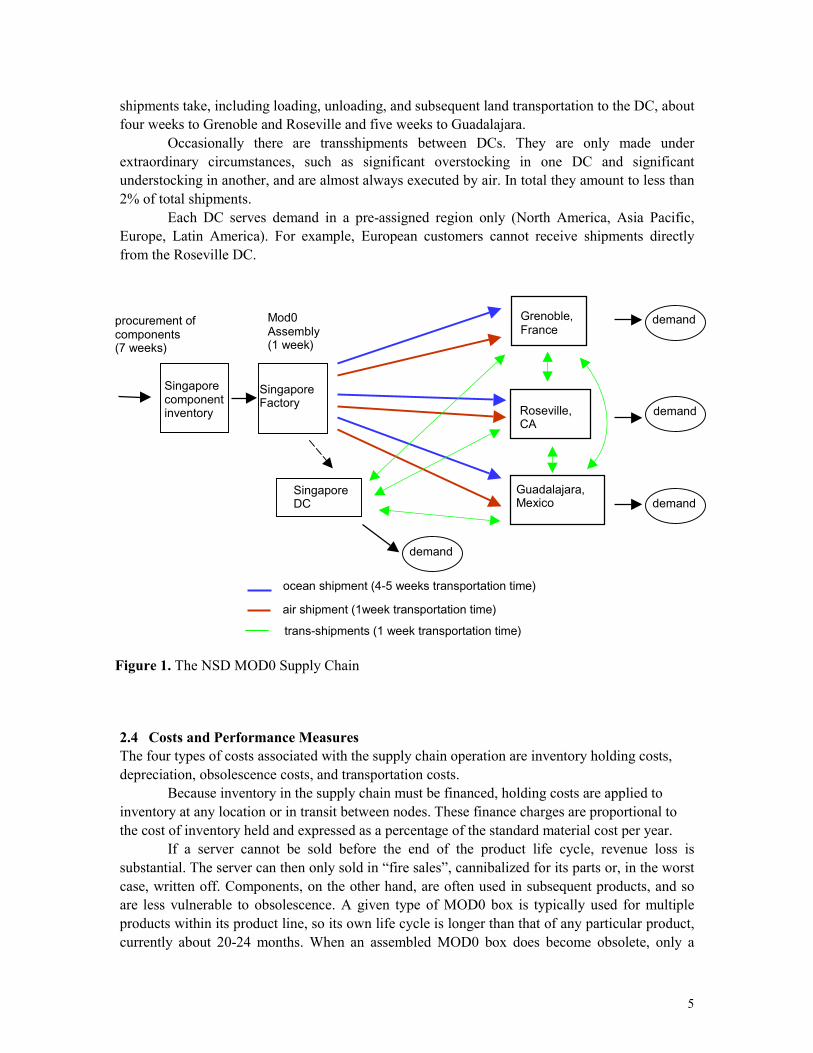
shipments take, including loading, unloading, and subsequent land transportation to the DC, aboutfour weeks to Grenoble and Roseville and five weeks to Guadalajara.

Occasionally there are transshipments between DCs. They are only made underextraordinary circumstances, such as significant overstocking in one DC and significantunderstocking in another, and are almost always executed by air. In total they amount to less than2% of total shipments.

Each DC serves demand in a pre-assigned region only (North America, Asia Pacific,Europe, Latin America). For example, European customers cannot receive shipments directlyfrom the Roseville DC.

2.4 Costs and Performance MeasuresThe four types of costs associated with the supply chain operation are inventory holding costs,depreciation, obsolescence costs, and transportation costs.

Because inventory in the supply chain must be financed, holding costs are applied toinventory at any location or in transit between nodes. These finance charges are proportional tothe cost of inventory held and expressed as a percentage of the standard material cost per year.

If a server cannot be sold before the end of the product life cycle, revenue loss issubstantial. The server can then only sold in “fire sales”, cannibalized for its parts or, in the worstcase, written off. Components, on the other hand, are often used in subsequent products, and soare less vulnerable to obsolescence. A given type of MOD0 box is typically used for multipleproducts within its product line, so its own life cycle is longer than that of any particular product,currently about 20-24 months. When an assembled MOD0 box does become obsolete, only a

SingaporeFactory

Singaporecomponentinventory

ocean shipment (4-5 weeks transportation time)

air shipment (1week transportation time)

procurement ofcomponents(7 weeks)

Grenoble,France

Roseville,CA

Guadalajara,Mexico

SingaporeDC

demand

demand

demand

trans-shipments (1 week transportation time)

demand

Mod0Assembly(1 week)

Figure 1. The NSD MOD0 Supply Chain

6

small fraction of its standard material cost can be recovered. Therefore, obsolescence cost equalto the difference of the original standard material cost and the recovered cost is incurred for everyassembled MOD0 box left at the end of its life cycle. Obsolescence cost for lower-levelcomponent inventory is much lower than obsolescence cost for assembled boxes since many ofthe parts can be used in successor products.

Prices for the components needed to build a MOD0 box decline rapidly over the courseof its lifecycle. Therefore, every MOD0 box held as inventory from one week to the next couldhave been built one week later at a lower price. The price difference is expressed in a depreciationcost applied to each unit of inventory in each period and location.

Transportation costs include freight cost, insurance, and costs of loading and unloading.Ocean shipment costs are charged per container shipped, whereas air shipment cost is charged perpallet. Ocean freight costs are about one-fifth of air freight costs. This cost advantage must beweighed against the higher inventory, depreciation and obsolescence cost associated with oceanshipments, as well as diminished agility as compared to air shipments.

The performance of the supply chain is currently measured by the off-the-shelfavailability for finished servers (the percentage of orders filled within a week or less) and the totalcost. Availability of components is currently not used of a performance measure.

2.5 Supply Chain OperationsAt the project’s inception, planners in the NSD World Wide Planning division in Santa Claracreated weekly production and shipment plans using rules that had been programmed intospreadsheets. Production orders and shipments were based on on-hand inventory targets for allthe DCs and the Singapore factory. When projected inventory on hand fell below the on-handtarget, an order was triggered. Planners generally chose air as the shipment mode; only when aMOD0 box was in surplus due to repeated high forecasts was an ocean shipment made. As aresult, the majority of shipments (over 65%) were made by air.

At that time, inventory targets were determined by using independent single-location,single-replenishment-mode inventory models at each location. A myopic order-up-to policy wascomputed based on the required service level. These calculations did not take into account non-stationarity of the demand, interactions between the DCs and the factory, nor potential savingsfrom utilizing different shipment modes appropriately. The end of the product life cycle washandled on an manual exception basis. Inventory targets were reduced during this phase, creatinglower availability (or longer response times) in order to avoid excessive obsolescence cost causedby leftover inventory.

At the same time, NSD was in the process of implementing Red Pepper as its planningengine. This system would automate the production and shipment decisions that planners wereusing spreadsheets to make. This automation would include the following rule for determining theallocation of air and sea shipments. First, let airLT and seaLT respectively denote the air and seashipment leadtimes for a given DC. For a given period t and this DC, Red Pepper compares theprojected inventory (based on on-hand and in-transit inventory and forecasts) in period t + airLTwith the DC’s target inventory for that period. Red Pepper triggers an air shipment to the DC ifthe projected inventory falls short of the target. Next, it considers making a sea shipment to theDC. To avoid making a sea shipment now that will adversely impact the ability to make airshipments that would arrive sooner, Red Pepper first “reserves” inventory at the factory that isneeded to make air shipments to all DCs that would arrive before the sea shipments in this period.If factory inventory remains after reserving for air shipments, then a sea order is triggered to

7

bring projected inventory in period t+seaLT up to the target for that period. Whenever there is ashortage of inventory at the factory, it is allocated to the DCs in proportion to the size of theirrequested shipments. This shipment mode selection rule is illustrated in Figure 2.

This selection rule, coupled with the relative magnitude of factory and DC targets,determines the fraction of shipments that are made by air. Thus, shipment decisions were notdirectly within the scope of the decision tool developed at HP Labs. Instead, these decisions wereto be a by-product of the recommended inventory strategy.

The total inventory of MOD0 boxes in the NSD supply chain, including in-transitbetween the factory and DCs, was approximately 8 weeks of supply when the project began. Theoff-the-shelf availability was approximately 85% for MOD0 boxes and 75% for servers. NSDhoped to ultimately satisfy 95% of demand for the finished product within one week response

time. Such an improvement would require, among other things outside the scope of this project, adramatic increase of MOD0 box availability.

2.6 Anticipated Project BenefitsThere were three ways in which the project team hoped they could reduce NSD’s supply chaincosts without compromising availability. The first was in redistribution of inventory. They hopedthat they might yield improved availability per unit of inventory by rebalancing inventorybetween the factory and DCs. The second way they hoped to improve operations was to reduceoverall supply chain inventory. A reduction of total MOD0 box inventory by 20% would save anequal percentage in inventory and depreciation cost annually. The third goal was increased usedof ocean shipments. By shifting the proportion of shipments from 65% air and 35% ocean to thereverse proportions, NSD anticipated savings of about 30% of freight costs. Of course, this

1. Make air shipments in period t. For each DC, determine desired air shipmentusing projected inventory and on-hand target in t+air LT. Make DC air shipments byallocating warehouse inventory in proportion to DC desired air shipments.

2. Plan for air shipments in t+1, …, t+seaLT-airLT-1. For each DC, reserve factoryinventory for air shipments that will arrive to meet DC targets in periods t+airLT+1, …,t+seaLT-1. Account for shipments that will arrive at the factory in time to make theseplanned air shipments.

3. Make sea shipments in period t. For each DC, Determine desired sea shipmentsto meet on-hand target in t+seaLT. Allocate unreserved factory inventory in proportionto DC desired sea shipments to make shipments.

t+ sea LTt t+ air LT

...

Figure 2. Selection of Shipment Mode

8

savings would be partly offset by higher inventory, depreciation and obsolescence cost; thistradeoff would have to be considered by the model.

Naturally, the potential cost savings was inversely related with service level goals. Thus, wewanted to develop an approach that would quantify the trade off between service level goals andcost, to enable NSD managers to strike the balance they desired.

The customers (re-sellers) have the right to return a certain percentage of the products theypreviously bought to the DC. Returns play a particularly important role close to the end of the lifecycle of the product since they contribute to a potential excess inventory and can incur highobsolescence cost for HP. On the other hand, even if inventory at the resellers is not returned tothe DC, price protection cost, which is based on the reseller inventory, constitutes a bigcontribution to NSD’s supply chain cost. An increase in service (shorter and more reliableresponse times) can impact both problems positively. If the DCs are more responsive resellers donot need to hold large inventory and returns as well as price protection expenses may drop.

2.7 The DataNSD World Wide Planning receives demand forecast on a monthly basis from NSD Marketing.These monthly forecasts are broken down into weekly “buckets” based on an empiricaldistribution of historical orders over the month. Using the bill of material, the component demandis determined. Historical data of actual demand back to 1996 is available. Forecasts have arelatively high error; coefficients of variation of 30-60% are not uncommon.

Cost data for freight and capital cost are available and relatively reliable. Depreciationcost and obsolescence cost can be estimated from historical data and specific business knowledgeavailable from the planners and the marketing department.

3 Related Literature

Three features of the NSD supply chain problem complicate finding an optimal inventory policy.The first is the existence of two replenishment modes. The second is the fact that the supply chainin question is a two-echelon distribution system. The third is the non-stationarity of demand. Eachof these features has been extensively studied independently. In what follows, we brieflysummarize the previous contributions in each of those areas.

A number of authors have considered single location inventory models with two supplymodes. One setting in which the form of the optimal inventory control policy has beencharacterized is under periodic review, with the critical assumption that the two modes’ leadtimesdiffer by exactly one period. Many authors, notably Fukuda (1960), Bulinskaya (1964a,b), Daniel(1962), Neuts (1964), Veinott (1966), Wright (1968), and Whittmore and Saunders (1977) havepresented results for this case. In those papers, it is shown that the optimal policy is ageneralization of the traditional order-up-to type policy, in which there are two order-up-to levelsin each period, for the short and long leadtime mode inventory positions, respectively.

Without the assumption that the leadtimes differ by one period, the form of the optimalpolicy is not known. Today’s shipment decision is certain to depend on the amount of inventoryon hand as well as the quantities due to arrive in each period between the short and long leadtimesfrom now. Moreover, it can be seen from a dynamic programming formulation of the problemthan an optimal strategy will not only depend on the total on-hand and pipeline inventory(inventory position) but also on the period in which what fraction of the pipeline inventory is

9

going to arrive. Work in this more general setting, both in periodic and continuous review, hasbeen done by authors such as Allen and D’Esopo (1968), Moinzadeh and Nahmias (1988),Moinzadeh and Schmidt (1991), Aggarwal and Moinzadeh (1994), Pyke and Cohen (1994), andChaing and Gutierrez (1996). These papers propose heuristic policies, the latter two in a multi-echelon setting. The work presented in this chapter also takes the approach of proposing a form ofheuristic policy that is more practical to implement than an optimal policy would be, andsearching for the best among such heuristic policies.

There are numerous papers on multi-echelon inventory systems with the same supply chainlayout as NSD’s. Optimal policies have not been characterized in this setting, but instead,practical policies have been proposed and evaluated. One exception is in serial systems, whereClark and Scarf (1960) gave the form of the optimal policy. Others such as Federgruen andZipkin (1984), Jackson (1988), and Graves (1996) propose heuristics for the periodic review case.Authors who consider continuous review (R,Q)-type policies in the multi-echelon setting includeSherbrooke (1968), Deuermeyer and Schwarz (1981), Graves (1985), Moinzadeh and Lee (1986),Lee and Moinzadeh (1987), Svoronos & Zipkin (1988), and Axsater (1993). This list is notexhaustive, but is hopefully representative of the literature in this area. Like previous approaches,our tactic is to consider a class of inventory policies that we expect to be effective and practical toimplement, and to search for the best policy within this class.

Finally, there have been many different models of nonstationary demand in single locationinventory models. The papers most relevant to NSD’s business and most related to the approachtaken here are those of Karlin (1960) and Veinott (1965). Karlin showed that order-up-to policiesare optimal in simple one node inventory systems even when demand is nonstationary, but theseorder-up-to levels aren’t easy to calculate in general. Veinott showed that if the demands werestochastically nondecreasing, then the optimal order-up-to levels were in fact the myopic ones(the newsvendor solution) and so are easy to compute.

4 The Model

In this section we describe the model used to represent NSD’s supply chain. In order to make themodel tractable, some simplifying assumptions were made. We felt that these assumptions weregeneral enough reflect the main features of the original supply chain closely, so that therecommendations made would remain valid.

Due to the relatively high capacity for assembly at the Singapore factory and the linearcost structure, different products do not interact in our model. For that reason we can treat each ofthe products in a separate one-product model.

4.1 Product FlowSince transshipments between DCs are rare and NSD does not wish to plan for them, we assumethat transshipments are not available as replenishment mechanisms. The supply chain resultingfrom this assumption is a distribution system. Customer demand is filled by the DC assigned forthe region, DCs receive their shipments from the Singapore factory, which in turn uses thecomponents from the Singapore inventory. Figure 3 shows the simplified supply chain layout.

Each inventory location in the supply chain is characterized by its replenishmentleadtimes, i.e. the time between the instant a replenishment order is placed until the orderedamount arrives in the inventory given the entity the order is demanded from has stock available.

10

For the DCs in France, the US and in Mexico, these leadtimes are the air and sea transportationtimes, which are inputs to the model. For the Singapore DC we assume the leadtime to be zerodue to its proximity to the factory. The leadtime for the Singapore component inventory is takento be the component procurement time plus the assembly time. This absorption of the assemblytime into the leadtime requires that assembly capacity is not restrictive.

4.2 DemandDemand occurs only at the DCs. We assume that the weekly demands can be described assequences of independent non-negative random variables. Weekly demands are not assumed to beidentically distributed; indeed they have been historically been highly non-stationary, due to lifecycle issues.

Non-negativity of demand is a technical assumption needed to make the mathematicalanalysis of the model more tractable. This assumption is not very restrictive for most of theproduct’s life where actual demands vastly exceed returns. In fact, if demand is determined assell-through+to3, non-negativity is virtually guaranteed.

Earlier investigations at NSD showed that Weibull distributions fit historical demand datareasonably well, and so we used them to model demand. The distribution parameters aredetermined by using the forecast as the distribution’s mean and the empirical coefficient ofvariation (obtained from historical data) as the distribution’s coefficient of variation. Our analysisdoes not crucially depend on this particular choice of distribution type. In fact, the software thatwas developed gives the user a choice of demand distributions to be specified in the input data.

3 Slightly simplistic, sell-through + to can be thought of as end-customer demand.

SingaporeFactory

Singaporecomponentinventory

ocean shipment (4-5 weeks transportation time)

air shipment (1week transportation time)

procurement ofcomponents andassembly(8 weeks)

Grenoble,France

Roseville,CA

Guadalajara,Mexico

SingaporeDC

demand

demand

demanddemand

Mod0 boxassembly

Figure 3. The Simplified Supply Chain

11

4.3 Cost and Performance MeasuresAlthough our analysis allows time- and location-dependent rates for holding and

depreciation, NSD chose to apply constant, universal rates to all inventories and products intransit. In particular, NSD lacked the data required to support a nonlinear depreciation rate model.Both costs are expressed as a constant percentage of the standard material cost.

A one-time obsolescence cost is applied to the products in inventory at the end of theplanning horizon. Currently the obsolescence cost is taken to be a fixed percentage of standardmaterial cost for all products, and it is only applied to DCs, since inventory there representsassembled MOD0s whereas factory inventory represents more versatile components. Thesechoices are not required for the analysis. In practice, the actual value that can be recovered at theend of a product’s life will vary from product to product, but it is difficult to estimate thesenumbers. We use the historical average for similar products.

Transportation cost is assumed to be proportionate to the amount shipped. The rate canvary across product, location and shipment mode. The proportionality assumption ignores theeffects of batching. This assumption is justified by the fact that NSD combines several differentproducts in one container, making batch sizes small compared to total volume shipped. Thispractice enables them to ship full containers only.

The performance of the system is measured by a type II service level for each of theproducts across all DCs. A type II service level is the mean of the fraction of demand which issatisfied off-the-shelf:

��

���

�=ductfor thePro Demand Total

Handon Stock from Satisfied Demand EProductλ . (1)

Our goal is to minimize the total cost incurred over the life cycle while guaranteeing a minimumservice level for each product.

5 Approach

In what follows we describe the approach we used to find cost-effective inventory managementpolicies. This approach, based on the model assumptions outlined above, is comprised of threemajor components. The first component is a refinement of the class of inventory strategies thatwe consider, and a parameterization of this class of strategies to afford efficient search amongthem. This is described in Section 5.1. The second element of our approach is a simulation enginethat emulates and evaluates how policies in our candidate class perform with respect to themetrics we have established. The simulation is described in Section 5.2 The third component, thesubject of Section 5.3, is a search procedure that relies on the parameterization of strategies andthe simulation results to select the best inventory strategy.

5.1 Candidate Inventory Replenishment Strategies

5.1.1 Implementable StrategiesIn every time period the inventory manager makes decisions about how much to order for thefactory and how much to ship to each of the DCs. All order and shipment quantities are non-negative. Naturally, the decision must be based only on the information available at the time it ismade; such decisions are called non-anticipative. In any period, the state of the supply chain is

12

completely described by the on-hand and in-transit quantities for each DC and the factory. Sincedemand is assumed to be independent between periods, there is an optimal feedback policy, i.e. apolicy that only depends on the current state rather than the complete history of the system.

Unfortunately, the optimal strategy is unlikely to have a simple structure, like that of aorder-up-to or a two-bin policy. Because there are two shipment modes with different lead times,the optimal replenishment decisions at the DCs will depend on the inventory on hand as well asshipment quantities due to arrive in several different periods. The limitations of the Red Peppersystem at that time prohibited implementing such complex rules.

Computing an optimal policy may also be difficult. To integrate our policy computationinto a decision support tool that would interface with the Red Pepper planning engine, lengthycomputation times would be unacceptable.

For these reasons, and because of the urgency of getting a working solution, we decidedto restrict our attention to the class of order-up-to policies. These policies are described by an on-hand inventory target for each location and each period. This choice is in accordance with currentpractice at NSD, and seemed most fitting to ensure a timely implementation of the project. Sincethe class of order-up-to policies does not, in general, contain the optimal policy, we plan toconsider more general policies at a later stage of the project.

5.1.2 Further Reduction of the Class of StrategiesA general order-up-to strategy requires inventory targets for the factory and each DC for eachperiod. For the current supply chain layout with one factory and four DCs, and a typical planninghorizon of 52 weeks, we would need 260 parameters to describe a order-up-to strategycompletely. To reduce complexity of the optimization problem, we propose a heuristic approachthat reduces the number of decision variables while still including a broad and sensible class ofstrategies. We deem a order-up-to strategy sensible if it meets the following requirements:• Targets should reflect changes in magnitude and variability of demand over time.4

• Service should be balanced over all DCs. A strategy that achieves good overall service levelin terms of Equation (1) but exhibits a significant imbalance in service between DCs is notacceptable.

• Service should be balanced over time. A strategy that achieves good overall service level butexhibits a significant imbalance in service over time5 is not acceptable. A controlled declinein service at the end of the life of a product may be desirable to avoid expensive excessinventory, see Section 5.1.3.

In what follows we describe a class of sensible strategies parameterized by two numbers,instead of one decision variable for each location and time period. As we will illustrate, these twonumbers correspond respectively to factory and DC service levels in independent single locationinventory models. To motivate this parameterization, recall that in a single location inventorymodel with one replenishment mode, the optimal inventory targets are determined by the servicelevel desired. These targets reflect the changing magnitude of demand as well as the changingvariability, expressed as its standard deviation, over time. The parameterization of policies allowsus to construct a sensible inventory strategy for the entire supply chain from targets derived fromsimple, single location models.

4 Restricting the search to stationary strategies, e.g., would simplify the analysis but seems like too strong arestriction for highly non-stationary demand of products like computers.

13

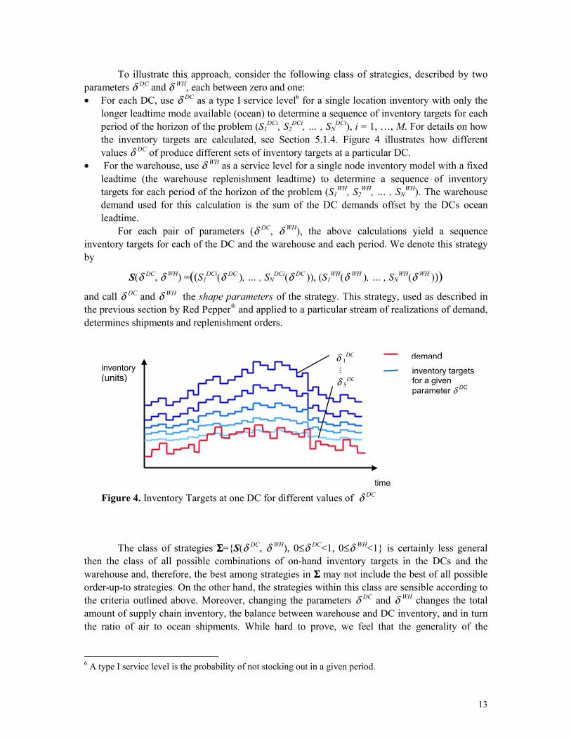
To illustrate this approach, consider the following class of strategies, described by twoparameters δ DC and δ WH, each between zero and one:• For each DC, use δ DC as a type I service level6 for a single location inventory with only the

longer leadtime mode available (ocean) to determine a sequence of inventory targets for eachperiod of the horizon of the problem (S1

DCi, S2DCi, … , SN

DCi), i = 1, …, M. For details on howthe inventory targets are calculated, see Section 5.1.4. Figure 4 illustrates how differentvalues δ DC of produce different sets of inventory targets at a particular DC.

• For the warehouse, use δ WH as a service level for a single node inventory model with a fixedleadtime (the warehouse replenishment leadtime) to determine a sequence of inventorytargets for each period of the horizon of the problem (S1

WH, S2WH, … , SN

WH). The warehousedemand used for this calculation is the sum of the DC demands offset by the DCs oceanleadtime.

For each pair of parameters (δ DC, δ WH), the above calculations yield a sequenceinventory targets for each of the DC and the warehouse and each period. We denote this strategyby

S(δ DC, δ WH) =((S1DCi(δ DC ), … , SN

DCi(δ DC )), (S1WH(δ WH ), … , SN

WH(δ WH )))and call δ DC and δ WH the shape parameters of the strategy. This strategy, used as described inthe previous section by Red Pepper and applied to a particular stream of realizations of demand,determines shipments and replenishment orders.

The class of strategies ΣΣΣΣ={S(δ DC, δ WH), 0≤δ DC<1, 0≤δ WH<1} is certainly less generalthen the class of all possible combinations of on-hand inventory targets in the DCs and thewarehouse and, therefore, the best among strategies in ΣΣΣΣ may not include the best of all possibleorder-up-to strategies. On the other hand, the strategies within this class are sensible according tothe criteria outlined above. Moreover, changing the parameters δ DC and δ WH changes the totalamount of supply chain inventory, the balance between warehouse and DC inventory, and in turnthe ratio of air to ocean shipments. While hard to prove, we feel that the generality of the

6 A type I service level is the probability of not stocking out in a given period.

time

inventory(units)

demandinventory targetsfor a givenparameter δ DC

δ 1DC

δ 5DC

Figure 4. Inventory Targets at one DC for different values of δ DC

�

14

strategies in ΣΣΣΣ ensures that the best strategy in ΣΣΣΣ will perform closely to the overall best strategyin terms of cost. In subsequent sections we will demonstrate how we select a strategy in ΣΣΣΣ.

5.1.3 Changing Service Level RequirementsUp to this point, we assumed the shape parameters of a particular strategy to be constant over thewhole horizon. This assumption corresponds to a constant level of service for all periods. Undersome circumstances it may be desirable to “distribute” service over the horizon unequally. Forexample, in the phase of new product introduction availability of the product might be crucial andone may want to achieve a higher level of service (lower probability of stock-outs) during thisphase. On the other hand, at the end of life one might be willing to sacrifice service in order toclear the supply chain of the product and minimize excess inventory. We accommodate theserequirements by introducing a service level shape that can be specified by the user. This servicelevel shape is a multiplicative parameter for each period. If the service level shape for period t isατ and for period t’ it is αt’ then the required service level in period t’ is αt’/ατ times the requiredservice level in period t. For a given sequence of service level shape parameters (αt)t=1, ..., Ν wemodify the class of candidate policy to

ΣΣΣΣα={Sα(δ DC, δ WH), 0≤δ DC<1, 0≤δ WH<1}

with

Sα(δ DC, δ WH) =((S1DCi(α1δ DC ), … , SN

DCi(αΝδ DC )), (S1WH(δ WH ), … , SN

WH(δ WH ))).

We apply the service level shape to the DC targets only for two reasons. The first reason is thatNSD incurs obsolescence cost only for excess inventory at the DCs. The second is that the levelof service at the DCs is a major management objective while the service at the factory is merely ameans to an end. Figure 5 depicts a typical service level shape for an end-of-life situation.

5.1.4 Calculating Inventory Policies in ΣΣΣΣIn this section we show how the inventory targets for a given shape parameter δ DC (respectively,δ WH) are calculated. Since the calculations are essentially the same for each DC and the

t

SLShape

MatureProduct

Ramp-Down End ofLife

Figure 5. Typical Service Level Shape

1

15

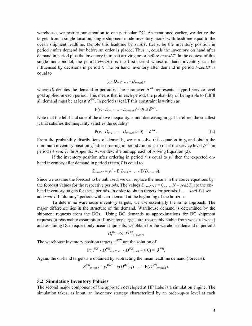
warehouse, we restrict our attention to one particular DC. As mentioned earlier, we derive thetargets from a single-location, single-shipment-mode inventory model with leadtime equal to theocean shipment leadtime. Denote this leadtime by seaLT. Let yt be the inventory position inperiod t after demand but before an order is placed. Thus, yt equals the inventory on hand afterdemand in period plus the inventory in transit arriving on or before t+seaLT. In the context of thissingle-mode model, the period t+seaLT is the first period whose on hand inventory can beinfluenced by decisions in period t. The on hand inventory after demand in period t+seaLT isequal to

yt - Dt+1- … - Dt+seaLT

where Dk denotes the demand in period k. The parameter δ DC represents a type I service levelgoal applied in each period. This means that in each period, the probability of being able to fulfillall demand must be at least δ DC. In period t+seaLT this constraint is written as

P(yt - Dt+1- … - Dt+seaLT> 0) ≥ δ DC.

Note that the left-hand side of the above inequality is non-decreasing in yt. Therefore, the smallestyt that satisfies the inequality satisfies the equality

P(yt - Dt+1- … - Dt+seaLT> 0) = δ DC. (2)

From the probability distributions of demands, we can solve this equation in yt and obtain theminimum inventory position yt

* after ordering in period t in order to meet the service level δ DC inperiod t + seaLT. In Appendix A. we describe our approach of solving Equation (2).

If the inventory position after ordering in period t is equal to yt* then the expected on-

hand inventory after demand in period t+seaLT is equal to

St+seaLT = yt* - E(Dt+1)- … - E(Dt+seaLT).

Since we assume the forecast to be unbiased, we can replace the means in the above equations bythe forecast values for the respective periods. The values St+seaLT, t = 0, …, N – seaLT, are the on-hand inventory targets for these periods. In order to obtain targets for periods 1, …, seaLT-1 weadd seaLT-1 “dummy” periods with zero demand at the beginning of the horizon.

To determine warehouse inventory targets, we use essentially the same approach. Themajor difference lies in the structure of the demand. Warehouse demand is determined by theshipment requests from the DCs. Using DC demands as approximations for DC shipmentrequests (a reasonable assumption if inventory targets are reasonably stable from week to week)and assuming DCs request only ocean shipments, we obtain for the warehouse demand in period t

DtWH =Σi DDCi

t+seaLTi.

The warehouse inventory position targets ytWH* are the solution of

P(ytWH

- DWH

t+1 - … - DWHt+whLT > 0) = δ WH.

Again, the on-hand targets are obtained by subtracting the mean leadtime demand (forecast):

SWHt+whLT = yt

WH* - E(DWHt+1)- … - E(DWH

t+whLT).

5.2 Simulating Inventory PoliciesThe second major component of the approach developed at HP Labs is a simulation engine. Thesimulation takes, as input, an inventory strategy characterized by an order-up-to level at each

16

location and time period in the horizon. (For example, this strategy could be one calculated as inSection 5.1.4 for a given pair of parameters (δ DC, δ WH )). It also requires demand distributioninformation (forecast, coefficient of variation, and distribution type) for each period and location,as well as structural supply chain data and costs. From this input, the program simulates how RedPepper would make shipment decisions given random demand drawn from the specifieddistributions. In the process, it measures the costs associated with a policy and its overall servicelevel (the percentage of demand satisfied immediately from stock) for a given demand outcome.This is repeated for many random demand scenarios, and the resulting costs and service levels forall runs are averaged. These averages are an approximation for the expected cost and service levelof the given set of inventory targets. Confidence intervals for these approximations are alsocomputed.

5.3 Searching for Optimal Policies In ΣΣΣΣSection 5.2 describes how we evaluate the expected cost and order fulfillment performance of anarbitrary set of inventory targets in the NSD supply chain. In particular, the simulation can beused to evaluate strategies in the class parameterized by δ DC and δ WH. In this section we discusshow we use the simulation to guide a search for the (δ DC, δ WH) expected to perform bestaccording to NSD’s cost and while meeting the overall service level criterion. To that end, definea point (δ DC, δ WH) in the grid as infeasible if its associated policy has an expected service levelbelow the desired one.

The pair (δ DC, δ WH) lies in the square [0,1) x [0,1). We begin by discretizing thisregion into a grid of arbitrarily small grid size. We use three observations to enableefficient search of points in this grid. The first observation is that if a given point (δ DC,δ WH) is infeasible, then any point smaller in both coordinates is also infeasible. Thisfollows from the fact that decreasing either parameter corresponds to decreasinginventory targets uniformly at all locations. (see Figure 6). The next two observationswere made based on empirical evidence rather than proven analytically. The second isthat for a fixed δ WH, the cost is empirically observed to be strictly increasing in the rangeof feasible δ DC. So the least feasible δ DC is best for a fixed δ WH. The third observation isthat for a fixed δ DC, the cost is quasi-convex in δ WH. This means that as you increase δ WH thecost never decreases after it increases.

1

1 δ D

δ W

feasible point

infeasible point

Figure 6. Search Grid for Shape Parameters

♦

♦

♦

♦

♦

♦

♦

♦

♦

♦

♦

♦

♦

♦

♦

♦

♦

♦

♦

♦

♦♦♦ ♦

17

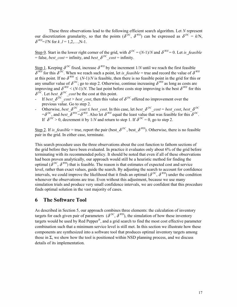
These three observations lead to the following efficient search algorithm. Let N representour discretization granularity, so that the points (δ DC, δ WH) can be expressed as δ DC = k/N,δ WH=l/N for k ,l = 1,2,…,N-1.

Step 0. Start in the lower right corner of the grid, with δ DC = (N-1)/N and δ WH = 0. Let is_feasible= false, best_cost = infinity, and best_δ DC_cost = infinity.

Step 1. Keeping δ DC fixed, increase δ WH by the increment 1/N until we reach the first feasibleδ WH for this δ DC. When we reach such a point, let is_feasible = true and record the value of δ WH

at this point. If no δ WH ≤ (N-1)/N is feasible, then there is no feasible point in the grid for this orany smaller value of δ DC; go to step 2. Otherwise, continue increasing δ WH as long as costs areimproving and δ WH < (N-1)/N. The last point before costs stop improving is the best δ WH for thisδ DC. Let best_δ DC_cost be the cost at this point.- If best_δ DC_cost > best_cost, then this value of δ DC offered no improvement over the

previous value. Go to step 2.- Otherwise, best_δ DC_cost ≤ best_cost. In this case, let best_δ DC_cost = best_cost, best_δ DC

=δ DC, and best_δ WH =δ WH. Also let δ WH equal the least value that was feasible for this δ DC.If δ DC > 0, decrement it by 1/N and return to step 1. If δ DC = 0, go to step 2.

Step 2. If is_feasible = true, report the pair (best_δ DC , best_δ WH). Otherwise, there is no feasiblepair in the grid. In either case, terminate.

This search procedure uses the three observations about the cost function to fathom sections ofthe grid before they have been evaluated. In practice it evaluates only about 6% of the grid beforeterminating with its recommended policy. It should be noted that even if all of these observationshad been proven analytically, our approach would still be a heuristic method for finding theoptimal (δ DC, δ WH) that is feasible. The reason is that estimates of expected cost and servicelevel, rather than exact values, guide the search. By adjusting the search to account for confidenceintervals, we could improve the likelihood that it finds an optimal (δ DC, δ WH) under the conditionwhenever the observations are true. Even without this adjustment, because we use manysimulation trials and produce very small confidence intervals, we are confident that this procedurefinds optimal solution in the vast majority of cases.

6 The Software Tool

As described in Section 5, our approach combines three elements: the calculation of inventorytargets for each given pair of parameters (δ DC, δ WH), the simulation of how these inventorytargets would be used by Red Pepper, and a grid search to find the most cost effective parametercombination such that a minimum service level is still met. In this section we illustrate how thesecomponents are synthesized into a software tool that produces optimal inventory targets amongthose in Σ, we show how the tool is positioned within NSD planning process, and we discussdetails of its implementation.

18

6.1 Program FlowThe flow of the program, depicted in Figure 7, is as follows:

(a) InitializationThe program reads the input data from files and uses the command line parameter options. Thesedata include:• supply chain characteristics (names and number of DCs, available shipment modes,

leadtimes)• demand characteristics (forecasts for each DC and each period, demand distribution type,

forecast error)• cost parameters (holding cost, depreciation cost, transportation cost for each DC and each

mode, obsolescence cost for each DC)• information about number of periods and the minimum overall service level requiredThe program then discretizes the demand distributions and produces a predefined number ofpseudo-random demand sequences (the length of each sequence is the number of periods of thehorizon) for each DC following the pre-specified distributions (type, forecast and error). Thesesequences are used later on to simulate demand.

(b) Determining Inventory TargetsAs outlined in Section 5.1.4, inventory targets are computed for each (δ DC, δ WH) by usingstandard single node/single mode inventory models. Solving equations of the form of (1) involvecalculating convolutions of the leadtime demand. This is done efficiently using Fast FourierTransforms.

(a) Initialize

(b) Compute policies in Σ:for δ WH = 0..1and δ DC = 0..1determine on-hand targets

use pure ocean shipment model withservice levels δ DC for DCs, use totaldemand offset by seaLT and δ WH forwarehouse

minimize cost,guarantee minimumservice level

• generate demand stream• emulate how Red Pepperwould use targets• record performance• average over many trials

selection algorithmdescribed in Section 5.3 (c) Optimize over δ DC, δ WH

Select a pairδ DC, δ WH

simulate, recordperformance

(d) Report best pairδ DC, δ WH

Figure 7. Program Flow

19

(c) SimulationFor each demand sequence generated in part (a), we simulate how the targets associated with agiven (δ DC, δ WH) are would be used by Red Pepper’s planning engine, as discussed in Section5.2. Service level, cost, and any other desired performance metrics are reported.(d) Grid SearchSteps (b) and (c) are repeated for values of δ DC and δ WH in a grid of values between zero and onewith pre-specified increments. The process for determining the sequence of (δ DC, δ WH) pairs isdescribed in Section 5.3.

(e) ReportHaving found the most cost effective feasible grid point, the program reports the associatedinventory targets, the achieved service level as well as the expected cost for this strategy. A vastarray supply chain performance metrics can also be reported, such as the percentage of shipmentsexpected to be made by air, expected backlogs, or decomposition of the expected total cost intoinventory, transportation, and obsolescence cost for each location.

6.2 Positioning of the ToolFigure 8 shows the proposed positioning of our tool within the NSD inventory managementprocess. As mentioned before, the purpose of the tool is to provide inventory targets, measured inweeks of supply7 (WOS). These targets will serve as inputs to the Red Pepper inventorymanagement tool.

While an automated data interchange between the HPL software tool and NSD’simplementation of Red Pepper is possible, we opted instead for web-based interfaces for input

7 Weeks of Supply (WOS) is a common measure of inventory targets and safety stock in inventorymanagement practice. At NSD, 1WOS is measured as next month’s demand divided by 4.3. Its purpose isto decouple targets from ever-changing forecasts and to give a sense of how long it is expected to take todeplete the inventory if no subsequent deliveries would occur. From a theoretical standpoint, in a non-stationary demand environment it would be more appropriate to express targets as a fraction of leadtimedemand.

Our Tool

calculatesoptimal WOSgoals

Red Pepper

plans shipmentsbased on WOStargets and itsrules

Input Data• forecasts• cost param.• service level• leadtimes WOS

Targets

ShipmentPlan

Figure 8. Positioning of the Tool

20

and output. This gives planners more control over how the tool’s recommended targets are used,and facilitates scenario analyses with respect to all input parameters of the program. The interfacewas developed by a group in HP called Supply Chain Information Systems (SCIS)

6.3 ImplementationThe program itself is written in C and runs on HPUX. It allows for batching several scenarios,taking advantage of the fact that certain calculations are common across scenarios. Several globaloptions can be set through command line parameters. These include the availability of only oneshipment mode, whether or not the end of life of the product coincides with the end of the modelhorizon or whether or not a particular service level shape should be applied.

7 Sample Results

This section contains a representative sample of results obtained for one of the MOD0 boxesbased on actual NSD data. The horizon of the model is 47 weeks. Two of the DCs have seashipments available (Roseville, CA and Grenoble, France). The others use only one shipmentmode. The results of the optimization and simulation with our tool are compared to the previousinventory targets used at NSD.

Figure 9 compares the cost for different minimum service levels, the current NSDstrategy (NSD Strategy) and the best strategy found by our tool that achieves the same servicelevel as the NSD strategy (NSD Service). Using our strategy, the simulation predicts a 27% costimprovement while maintaining the current service level.

Cost vs. Service Level

0.951

0.970

0.980

0.990

0.975 0.975

0.960

0.0

0.5

1.0

1.5

2.0

2.5

3.0

3.5

4.0

4.5

95% 96% 97% 98% 99% NSD Policy NSD Service Scenario

Cost (in $M

)

0.93

0.94

0.95

0.96

0.97

0.98

0.99

1

Service Level

Cost Service Level

Figure 9. Cost for Dfferent Scenarios

21

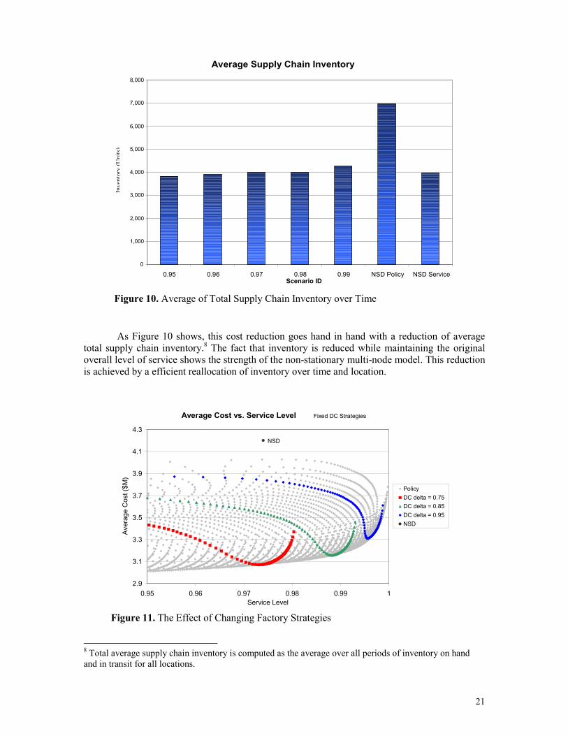
As Figure 10 shows, this cost reduction goes hand in hand with a reduction of averagetotal supply chain inventory.8 The fact that inventory is reduced while maintaining the originaloverall level of service shows the strength of the non-stationary multi-node model. This reductionis achieved by a efficient reallocation of inventory over time and location.

8 Total average supply chain inventory is computed as the average over all periods of inventory on handand in transit for all locations.

Average Supply Chain Inventory

0

1,000

2,000

3,000

4,000

5,000

6,000

7,000

8,000

0.95 0.96 0.97 0.98 0.99 NSD Policy NSD ServiceScenario ID

Inve

ntor

y(U

nits

)

Figure 10. Average of Total Supply Chain Inventory over Time

Average Cost vs. Service Level Fixed DC Strategies

2.9

3.1

3.3

3.5

3.7

3.9

4.1

4.3

0.95 0.96 0.97 0.98 0.99 1Service Level

Aver

age

Cos

t ($M

)

PolicyDC delta = 0.75DC delta = 0.85DC delta = 0.95NSD

NSD

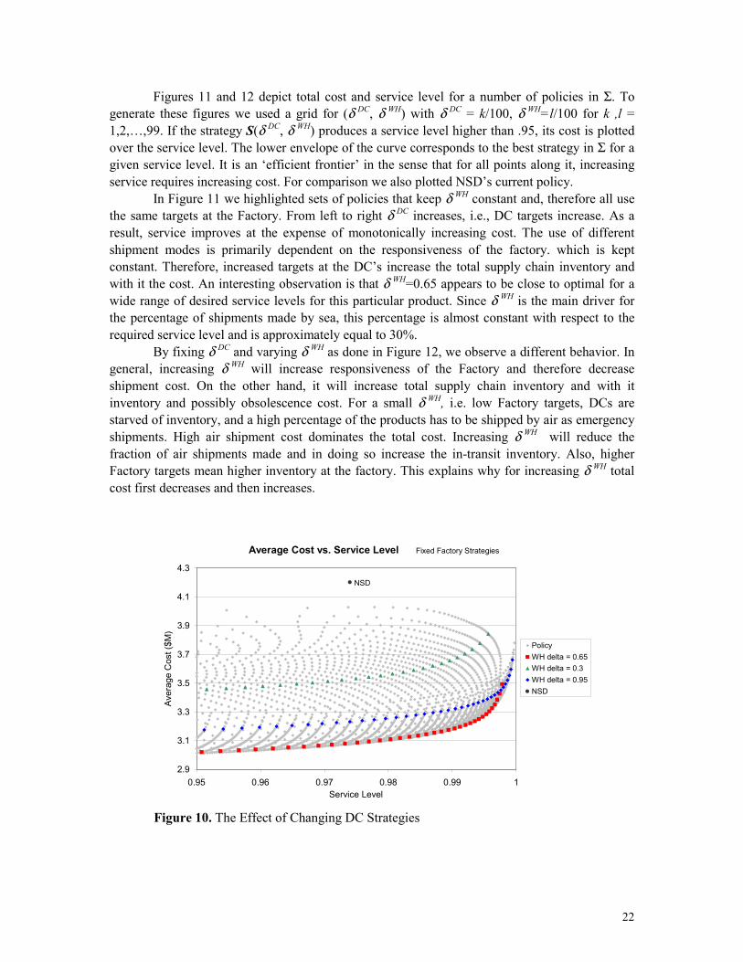
Figure 11. The Effect of Changing Factory Strategies

22

Figures 11 and 12 depict total cost and service level for a number of policies in Σ. Togenerate these figures we used a grid for (δ DC, δ WH) with δ DC = k/100, δ WH=l/100 for k ,l =1,2,…,99. If the strategy S(δ DC, δ WH) produces a service level higher than .95, its cost is plottedover the service level. The lower envelope of the curve corresponds to the best strategy in Σ for agiven service level. It is an ‘efficient frontier’ in the sense that for all points along it, increasingservice requires increasing cost. For comparison we also plotted NSD’s current policy.

In Figure 11 we highlighted sets of policies that keep δ WH constant and, therefore all usethe same targets at the Factory. From left to right δ DC increases, i.e., DC targets increase. As aresult, service improves at the expense of monotonically increasing cost. The use of differentshipment modes is primarily dependent on the responsiveness of the factory. which is keptconstant. Therefore, increased targets at the DC’s increase the total supply chain inventory andwith it the cost. An interesting observation is that δ WH=0.65 appears to be close to optimal for awide range of desired service levels for this particular product. Since δ WH is the main driver forthe percentage of shipments made by sea, this percentage is almost constant with respect to therequired service level and is approximately equal to 30%.

By fixing δ DC and varying δ WH as done in Figure 12, we observe a different behavior. Ingeneral, increasing δ WH will increase responsiveness of the Factory and therefore decreaseshipment cost. On the other hand, it will increase total supply chain inventory and with itinventory and possibly obsolescence cost. For a small δ WH, i.e. low Factory targets, DCs arestarved of inventory, and a high percentage of the products has to be shipped by air as emergencyshipments. High air shipment cost dominates the total cost. Increasing δ WH will reduce thefraction of air shipments made and in doing so increase the in-transit inventory. Also, higherFactory targets mean higher inventory at the factory. This explains why for increasing δ WH totalcost first decreases and then increases.

Average Cost vs. Service Level Fixed Factory Strategies

2.9

3.1

3.3

3.5

3.7

3.9

4.1

4.3

0.95 0.96 0.97 0.98 0.99 1Service Level

Aver

age

Cos

t ($M

)

PolicyWH delta = 0.65WH delta = 0.3WH delta = 0.95NSD

NSD

Figure 10. The Effect of Changing DC Strategies

23

Since the inception of this project our results have been implemented at NSD. Total supplychain inventory has been reduced significantly without jeopardizing off-the-shelf availability.Transportation cost has been reduced by more extensive use of ocean shipments.

8 Conclusion

Prior to the commencement of this project, NSD used simple single-location, single-supply-modeinventory models to aid in the determination of inventory targets. These models also assumedemand to be stationary. This chapter describes an approach that models the true two-tier, two-mode nature of the NSD supply chain and the interaction between these tiers. In particular, ittakes into account the effects of shortages at the warehouse and the competition between DCs forwarehouse supply. The model also accommodated product life-cycles by not requiring demand orservice level goals to be stationary over time.

Our results demonstrate that this approach produced more effective inventory strategiesthan their previous method. This can explained by the fact that both the amount of supply chaininventory and its distribution between the factory and the DCs are critically important indetermining overall costs and level of service. NSD’s previous approach to finding inventorystrategies was not general enough to address these factors.

24

Acknowledgements:The authors would like to acknowledge the support that was critical for the success of the project.During his tenure at HP Labs, Krishna Venkatraman was an invaluable contributor to all aspectsof this work. We will not forget him, even if he gets rich. Shailendra Jain, the manager of theDecision Technology Department at HP Labs, was instrumental in getting the project establishedand seeing it along. Our partners Roger Smith, Zawadi Pettes and Steve Kohler at NSD helpedtremendously in identifying and refining the model and provided continuous feedback. We alsothank Jeff McKibben, Amy Shao, Keiichiro Ichiryu, Darren Johnson, and Thomas Zscherpel inHP’s Supply Chain Information Systems for helping us to build a graphical user interface for ourtool.

25

References

Aggarwal, P., K. Moinzedeh, 1994. Order expedition in multi-echelon production/distributionsystems. IIE Transactions 26, 86-96

Allen, S., D. Esopo, 1968. An ordering policy for stock when delivery can be expedited.Operations Res. 16, 830-833.

Axsater, S., 1993. Exact and approximate evaluation of two-level inventory systems. OperationsRes. 41, 777-785.

Bulinskaya, E., 1964. Some results concerning optimal inventory policies. Theor. ProbabilityAppl. 9, 389-403.

Bulinskaya, E., 1964. Steady-state solutions in problems of optimal inventory control. Theor.Probability Appl. 9, 502-507.

Chiang, C., G. Gutierrez, Periodic review inventory system with two supply modes. EuropeanJournal of Operational Research 94, 527-547.

Clark, A.J., Scarf, H., 1960. Optimal policies for a multi-echelon inventory problem.Management Sci. 6, 475-490.

Daniel, K., 1962. A delivery-lag inventory model with emergency order. Multistage InventoryModels and Techniques (Chapter 2), Scarf, Gilford, Shelly (eds.) Stanford University Press,Stanford, California.

Deuermeyer, B., L. Schwarz, 1981. A model for the analysis of system service level in warehouseretailer distribution system. Multi-Level Production/Inventory Control Systems: Theory andPractice, Schwartz, L. (Ed.), TIMS Studies in Management Science, 16, Amsterdam, North-Holland, 51-67.

Federgruen, A., P. Zipkin, 1984. Allocation policies and cost approximations for multilocationinventory systems. Nav Res Logist Q 31, 97-129.

Federgruen, A., P. Zipkin, 1984. Approximations of dynamic, multilocation production andinventory problems. Management Sci. 30, 69-84.

Fukuda, Y., 1960. Optimal policies for the inventory problem with negotiable leadtime.Management Sci. 10, 690-708.

Graves, S., 1985. A multi-echelon inventory model for a repairable item with one-for-onereplenshment. Management Sci. 31, 1247-1256.

Graves, S., 1996. Multiechelon inventory model with fixed replenishment intervals. ManagementSci 42, 1-18.

Jackson, P., 1988. Stock allocation in a two-echelon distribution system, or 'what to do until yourship comes in'. Management Sci 34, 880-895.

26

Karlin, S., 1960. Dynamic inventory policy with varying stochastic demands. Management Sci. 6,231-258

Moinzedeh, K., H. Lee, 1986. Batch size and stocking levels in multi-echelon repairable systems.Management Sci. 32, 1567-1581.

Lee, H., K. Moinzadeh 1987. Two parameter approximations for multi-echelon repairableinventory models with batch ordering policy. IIE Transactions 19, 140-149

Moinzedeh, K., S. Nahmias, 1988. A continuous review mode for an inventory system with twosupply modes. Management Sci 34, 761-773.

Moinzadeh, K., C. Schmidt, 1991. An (S-1,S) inventory system with emergency orders.Operations Res. 39, 308-321.

Neuts, M., 1964. An inventory model with an optional time lag. SIAM 12, 179-185.

Pyke, D., M. Cohen, 1994. Multiproduct integrated production-distribution systems.Eur. J. Oper. Res. 74 18-49.

Sherbrooke, C., 1968. METRIC: Multi-echelon technique for recoverable item control.Operations Res. 16, 122-141.

Svoronos, A., P. Zipkin, 1988. Estimating the performance of multi-level inventory systems.Operations Res. 36, 57-72.

Veinott, A., 1965. Optimal policy for a multi-product, dynamic, nonstationary inventory problem.Management Sci. 12, 206-222.

Veinott, A., 1966. The status of mathematical inventory. Management Sci. 12, 745-777.

Whittmore, A., S. Saunders, 1977. Optimal inventory under stochastic demand with two supplyoptions. SIAM J. Appl. Math. 32, 293-305.

Wright, G. 1968. Optimal policies for a multi-product inventory system with negotiableleadtimes. Naval Res. Logist. Q. 15, 375-401.

27

Appendix A. Solving Equation (2)We rewrite Equation (2) as

.)P( 1DC

seaLTittt DD Dy δ=+++> ++ � (3)

Let Φ(x) be the cumulative distribution function of the sum Dt+ … + Dt+seaLT. Then we can write(3) as

1-Φ ( yt ) = δ DC (4)

or equivalently

yt = Φ -1(δ DC ). (5)

Let Φt(x),…, Φt+seaLT(x) be the cumulative distribution functions of Dt, Dt+1,…, Dt+seaLT,respectively. Then, the function Φ(x) is the convolution9 of these functions:

).()()()( 1 xxxx seaLTttt ++ Φ∗∗Φ∗Φ=Φ � (6)

While Equation (6) defines the function Φ(x), using only the definition of the convolution it israther difficult to compute it. We use the following well-known theorem:

THEOREM 1. Let F(f ), F(g) denote the Fourier Transform10 of the functions f and g. Then

F(f *g)=F(f ) F(g).

Using Theorem 1 we can write (5) as

( ) ( ) ( )( ).)(F)(F)(FF)( 1-1 xxxx seaLTttt ++ Φ××ΦΦ=Φ �

(7)

Using readily available C code for Fast Fourier Transforms (FFT) and its inverse the functionΦ(x) can be computed relatively quickly. Applying (4) yields the desired order-up-to-levels.

9 The convolution Ψ(x)=Φ(x)*Θ(x) of two (differentiable) cumulative distribution functions Φ(x) and Θ(x)is defined as

.d)(')(:)(0

zzzxxx

Θ−Φ=Ψ �10 The Fourier Transform F(f ) is defined as

�∞

∞−

−= xxfetf itx d)(:))((F