network reliability assessment - koç hastanesihome.ku.edu.tr/~indr343/files/chapter 29 (markov...
TRANSCRIPT

1
INDR 343
Stochastic Models
Department of Industrial Engineering
Koç University
Chapter 29
Markov Chains
Süleyman Özekici
ENG 119, Ext: 1723
S. Özekici INDR 343 Stochastic Models 2
Course Topics
• Markov Chains (Chapter 29)
• Queueing Models (Chapter 17)
• Inventory Models (Chapter 18)
• Markov Decision Models (Chapter 19)
2
S. Özekici INDR 343 Stochastic Models 3
Markov Chains and Processes
• Stochastic processes
• Introduction to Markov chains
• Transient analysis
• Classsification of states
• Ergodic and potential analysis of MC
• Introduction to Markov processes
• Ergodic and potential analysis of MP
S. Özekici INDR 343 Stochastic Models 4
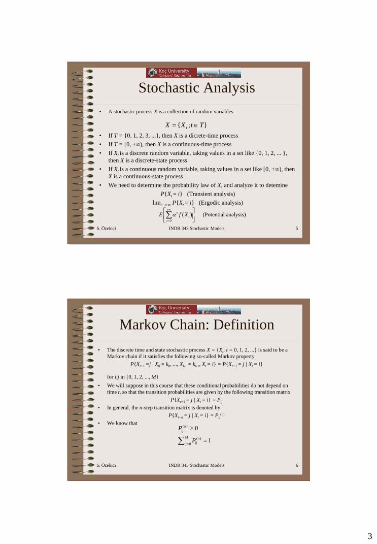
Stochastic Processes
• Many stochastic models in operations research are represented using a collection of
random variables that are indexed by time, so that
Xt = state of the system at time t
• Some examples are
– Xt = the number of shoppers who arrived at a supermarket until time t
– Xt = the amount of inventory in stock at the end of week t
– Xt = the number of patients in the emergency room of an hospital at
time t
– Xt = the price of a share of common stock that is traded at Istanbul
Stock Exchange at the close of day t
– Xt = the functional state of a workstation at time t
– Xt = the number of vehicles that arrive at the Boğaziçi bridge during day t
– Xt = the time of arrival of the tth customer to a bank during a given day
– Xt = the number of wins of a soccer team in t matches played
3
S. Özekici INDR 343 Stochastic Models 5
Stochastic Analysis
• A stochastic process X is a collection of random variables
• If T = {0, 1, 2, 3, ...}, then X is a dicrete-time process
• If T = [0, +∞), then X is a continuous-time process
• If Xt is a discrete random variable, taking values in a set like {0, 1, 2, ... },
then X is a discrete-state process
• If Xt is a continuous random variable, taking values in a set like [0, +∞), then
X is a continuous-state process
• We need to determine the probability law of X, and analyze it to detemine
P{Xt = i} (Transient analysis)
limt+∞ P{Xt = i} (Ergodic analysis)
};{ TtXX t
0
( ) (Potential analysis)t
t
t
E f X+
S. Özekici INDR 343 Stochastic Models 6
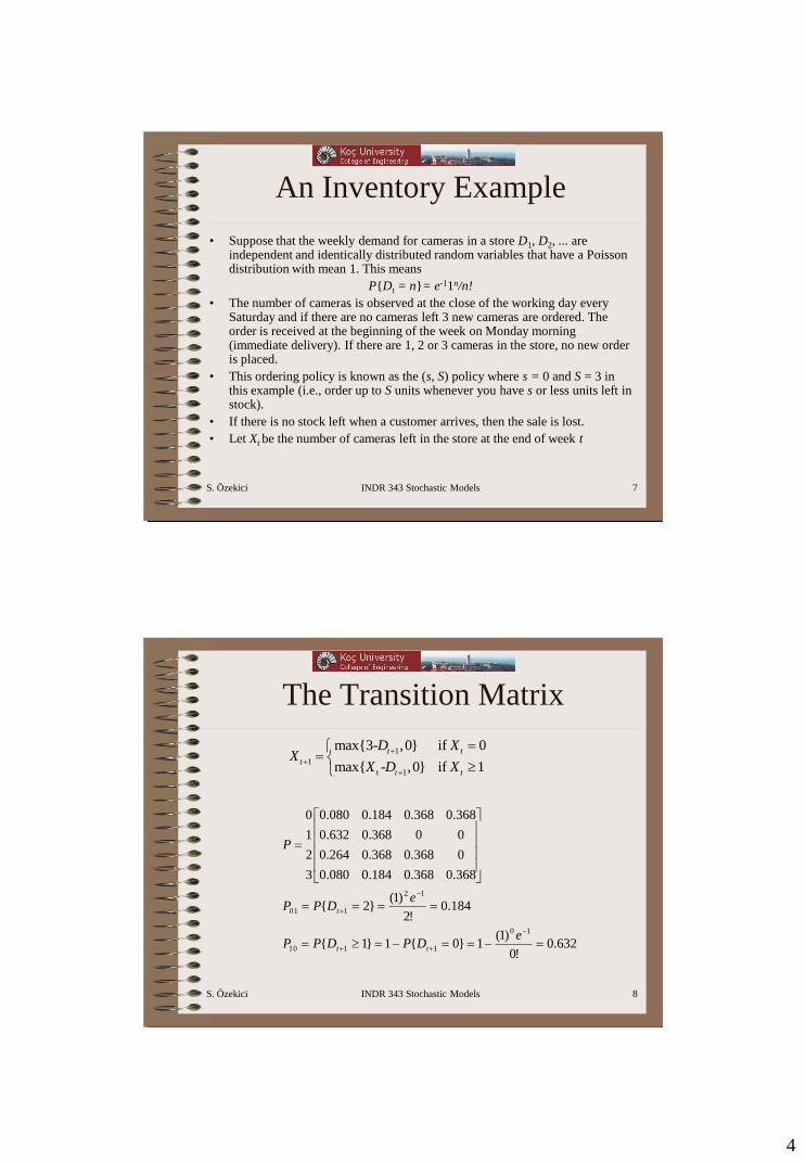
Markov Chain: Definition
• The discrete time and state stochastic process X = {Xt; t = 0, 1, 2, ...} is said to be a
Markov chain if it satisfies the following so-called Markov property
P{Xt+1 =j | X0 = k0, ..., Xt-1 = kt-1, Xt = i} = P{Xt+1 = j | Xt = i}
for i,j in {0, 1, 2, ..., M} • We will suppose in this course that these conditional probabilities do not depend on
time t, so that the transition probabilities are given by the following transition matrix
P{Xt+1 = j | Xt = i} = Pij
• In general, the n-step transition matrix is denoted by
P{Xt+n = j | Xt = i} = Pij(n)
• We know that
1
0
0
)(
)(
M
j
n
ij
n
ij
P
P
4
S. Özekici INDR 343 Stochastic Models 7
An Inventory Example
• Suppose that the weekly demand for cameras in a store D1, D2, ... are independent and identically distributed random variables that have a Poisson distribution with mean 1. This means
P{Dt = n}= e-11n/n!
• The number of cameras is observed at the close of the working day every Saturday and if there are no cameras left 3 new cameras are ordered. The order is received at the beginning of the week on Monday morning (immediate delivery). If there are 1, 2 or 3 cameras in the store, no new order is placed.
• This ordering policy is known as the (s, S) policy where s = 0 and S = 3 in this example (i.e., order up to S units whenever you have s or less units left in stock).
• If there is no stock left when a customer arrives, then the sale is lost.
• Let Xt be the number of cameras left in the store at the end of week t
S. Özekici INDR 343 Stochastic Models 8
1
1
t 1
max{3- ,0} if 0
max{ - ,0} if 1
t t
t
t t
D XX
X D X
+
+
+
The Transition Matrix
632.0!0
)1(1}0{1}1{
184.0!2
)1(}2{
368.0368.0184.0080.0
0368.0368.0264.0
00368.0632.0
368.0368.0184.0080.0
3
2
1
0
10
1110
12
101
++
+
eDPDPP
eDPP
P
tt
t
5
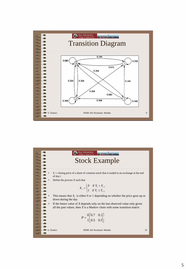
S. Özekici INDR 343 Stochastic Models 9
Transition Diagram
S. Özekici INDR 343 Stochastic Models 10
Stock Example
• Yt = closing price of a share of common stock that is traded in an exchange at the end
of day t
• Define the process X such that
• This means that Xt is either 0 or 1 depending on whether the price goes up or
down during the day
• If the future value of X depends only on the last observed value only given
all the past values, then X is a Markov chain with some transition matrix
if1
if0
1
1
tt
tt
tYY
YYX
5.05.0
3.07.0
1
0P
6
S. Özekici INDR 343 Stochastic Models 11
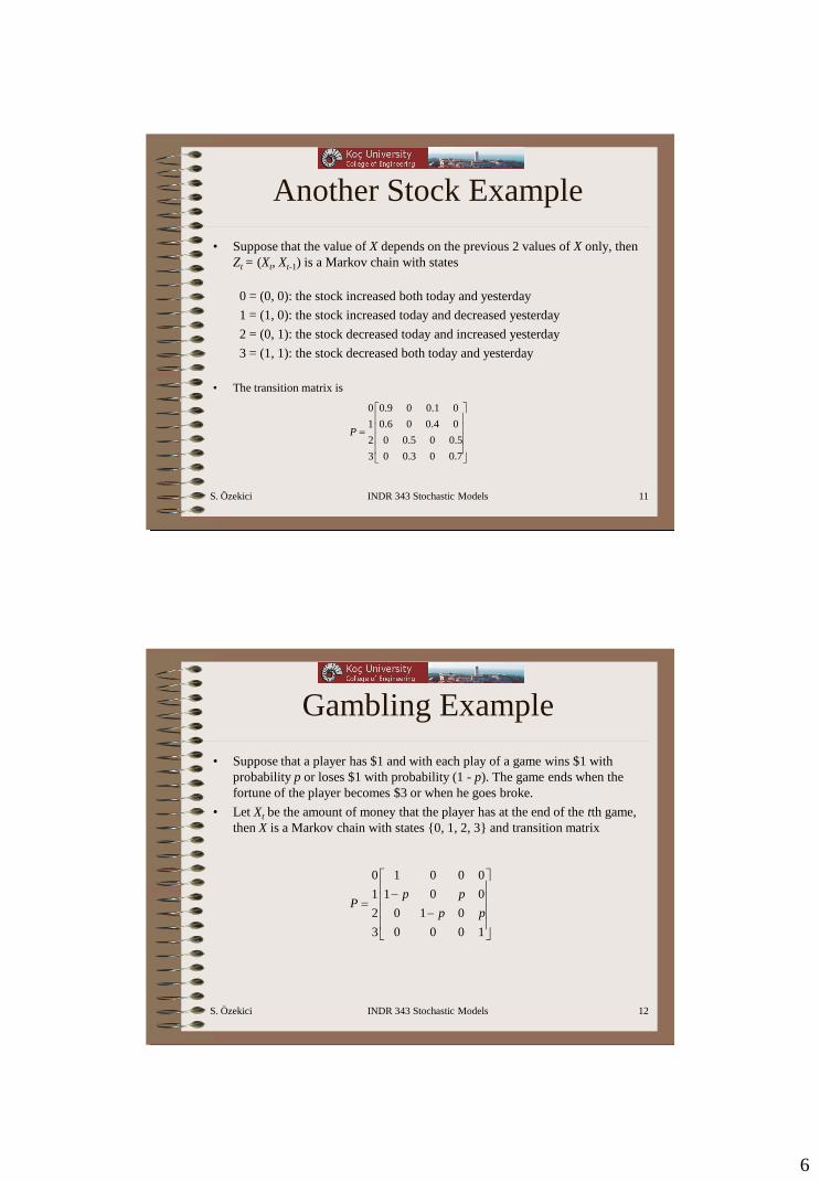
Another Stock Example
• Suppose that the value of X depends on the previous 2 values of X only, then
Zt = (Xt, Xt-1) is a Markov chain with states
0 = (0, 0): the stock increased both today and yesterday
1 = (1, 0): the stock increased today and decreased yesterday
2 = (0, 1): the stock decreased today and increased yesterday
3 = (1, 1): the stock decreased both today and yesterday
• The transition matrix is
7.003.00
5.005.00
04.006.0
01.009.0
3
2
1
0
P
S. Özekici INDR 343 Stochastic Models 12
Gambling Example
• Suppose that a player has $1 and with each play of a game wins $1 with
probability p or loses $1 with probability (1 - p). The game ends when the
fortune of the player becomes $3 or when he goes broke.
• Let Xt be the amount of money that the player has at the end of the tth game,
then X is a Markov chain with states {0, 1, 2, 3} and transition matrix
1000
010
001
0001
3
2
1
0
pp
ppP
7
S. Özekici INDR 343 Stochastic Models 13
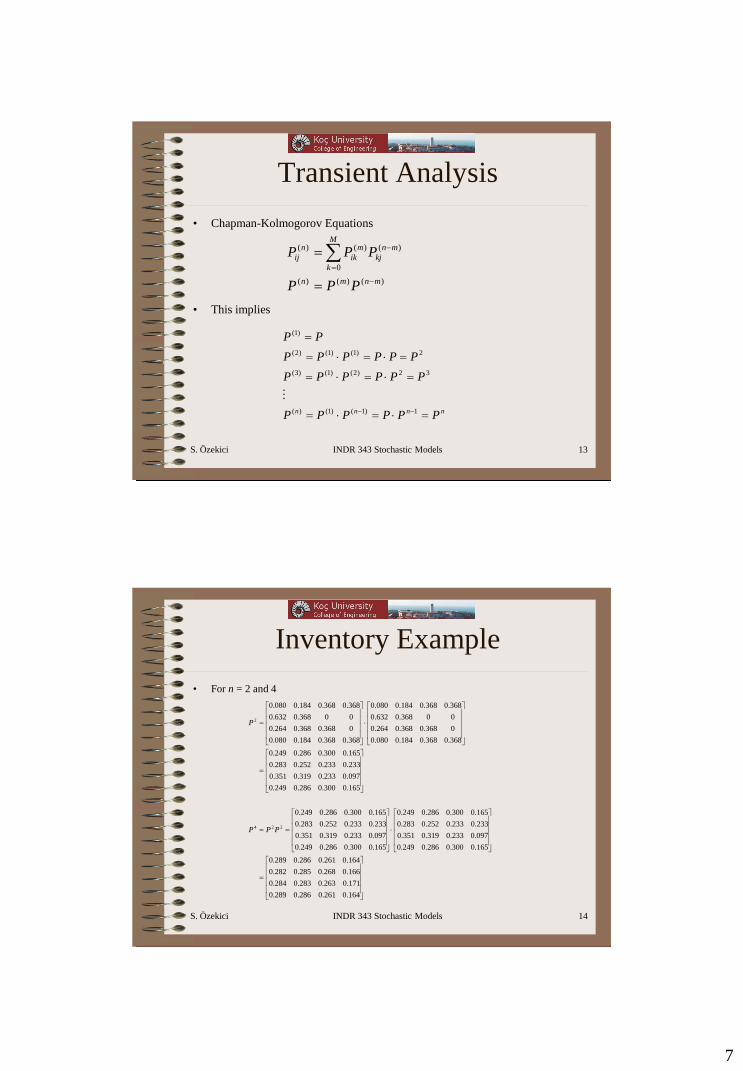
Transient Analysis
• Chapman-Kolmogorov Equations
• This implies
)()()(
0
)()()(
mnmn
M
k
mn
kj
m
ik
n
ij
PPP
PPP
nnnn PPPPPP
PPPPPP
PPPPPP
PP
1)1()1()(
32)2()1()3(
2)1()1()2(
)1(
S. Özekici INDR 343 Stochastic Models 14
Inventory Example
• For n = 2 and 4
164.0261.0286.0289.0
171.0263.0283.0284.0
166.0268.0285.0282.0
164.0261.0286.0289.0
165.0300.0286.0249.0
097.0233.0319.0351.0
233.0233.0252.0283.0
165.0300.0286.0249.0
165.0300.0286.0249.0
097.0233.0319.0351.0
233.0233.0252.0283.0
165.0300.0286.0249.0
165.0300.0286.0249.0
097.0233.0319.0351.0
233.0233.0252.0283.0
165.0300.0286.0249.0
368.0368.0184.0080.0
0368.0368.0264.0
00368.0632.0
368.0368.0184.0080.0
368.0368.0184.0080.0
0368.0368.0264.0
00368.0632.0
368.0368.0184.0080.0
224
2
PPP
P
8
S. Özekici INDR 343 Stochastic Models 15
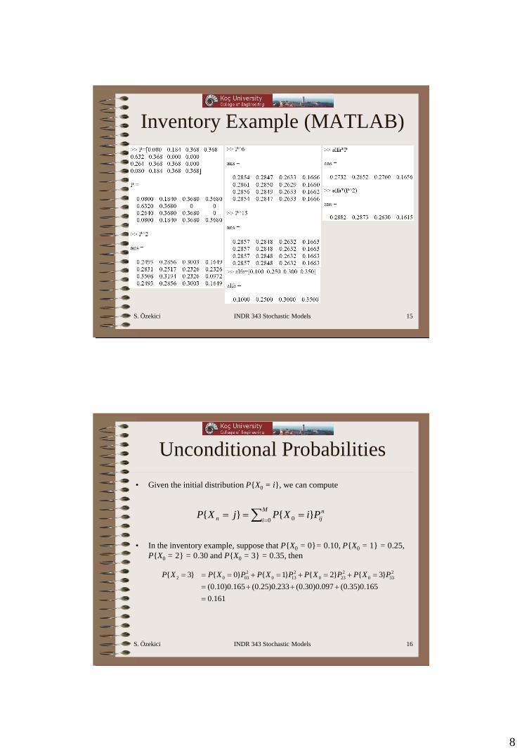
Inventory Example (MATLAB)
S. Özekici INDR 343 Stochastic Models 16
Unconditional Probabilities
• Given the initial distribution P{X0 = i}, we can compute
• In the inventory example, suppose that P{X0 = 0}= 0.10, P{X0 = 1} = 0.25,
P{X0 = 2} = 0.30 and P{X0 = 3} = 0.35, then
M
i
n
ijn PiXPjXP0 0 }{}{
2 2 2 2
2 0 03 0 13 0 23 0 33{ 3} { 0} { 1} { 2} { 3}
(0.10)0.165 (0.25)0.233 (0.30)0.097 (0.35)0.165
0.161
P X P X P P X P P X P P X P + + +
+ + +

9
S. Özekici INDR 343 Stochastic Models 17
Classification of States
• State j is accessible from state i if Pijn > 0 for some n
• States i and j communicate if j is accessible from i and i is accessible from j
• A class consists of all states that communicate with each other
• The Markov chain is irreducible if it consists of a single class, or if all states
communicate
• State i is transient if, upon entering this state, the process may never return to it
• State i is recurrent if, upon entering this state, the process definitely will return to it
• State i is absorbing if, upon entering this state, the process will never leave it
• State i is periodic with period t >1, if Piin = 0 for all values of n other than t, 2t, 3t, 4t,
...; otherwise, it is aperiodic
• State i is ergodic if it is recurrent and aperiodic
• A Markov chain is ergodic if all of its states are ergodic
S. Özekici INDR 343 Stochastic Models 18
Examples
• In the inventory and stock examples, the Markov chain is ergodic
• In the gambling example, the Markov chain is not ergodic. States 0 and 3 are
both absorbing, and states 1 and 2 are transient.
• In the following example,
– State 2 is absorbing
– States 0 and 1 form a class of recurrent and aperiodic states
– States 3 and 4 are transient
00001
03/23/100
00100
0002/12/1
0004/34/1
4
3
2
1
0
P
10
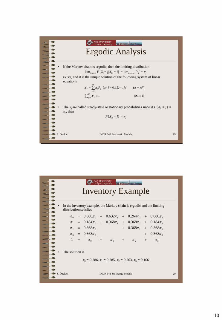
S. Özekici INDR 343 Stochastic Models 19
Ergodic Analysis
• If the Markov chain is ergodic, then the limiting distribution
limt+∞ P{Xt = j|X0 = i} = limt+∞ Pijt = πj
exists, and it is the unique solution of the following system of linear
equations
• The πj are called steady-state or stationary probabilities since if P{X0 = j} =
πj , then
P{Xn = j} = πj
)1( 1
)( ,,2,1,0for
0
0
1
M
j j
M
i
ijij PMjP
S. Özekici INDR 343 Stochastic Models 20
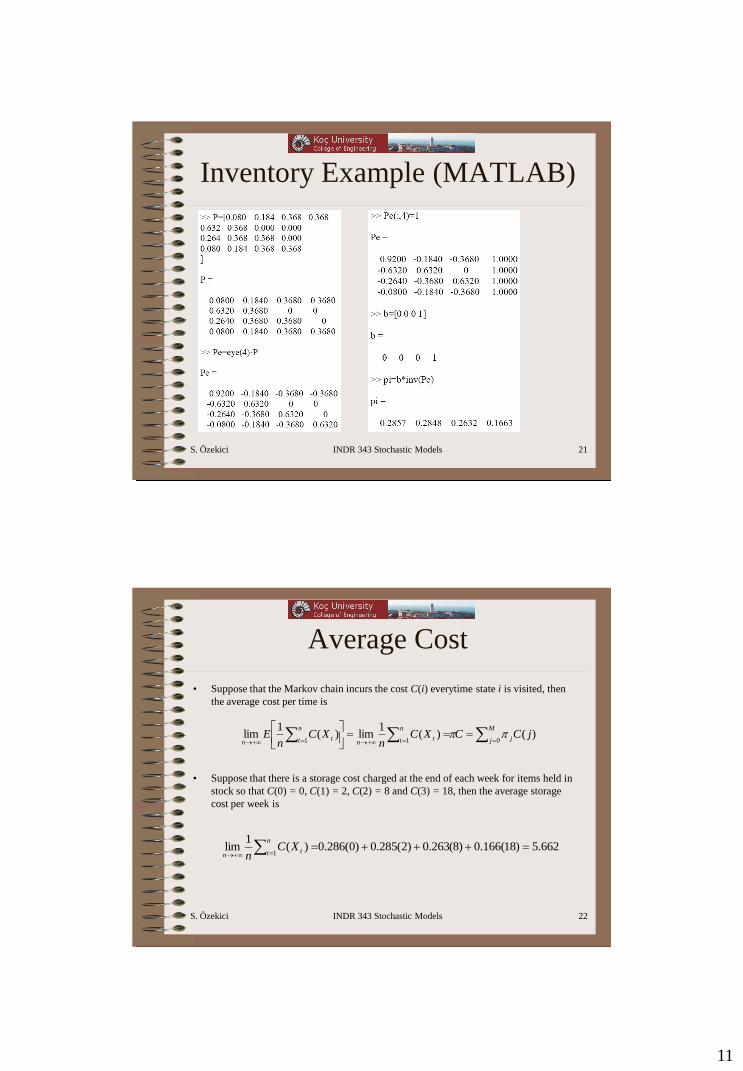
Inventory Example
• In the inventory example, the Markov chain is ergodic and the limiting distribution satisfies
• The solution is
π0 = 0.286, π1 = 0.285, π2 = 0.263, π3 = 0.166
3210
303
3202
32101
32100
1
368.0368.0
368.0368.0368.0
184.0368.0368.0184.0
080.0264.0632.0080.0
+++
+
++
+++
+++
11
S. Özekici INDR 343 Stochastic Models 21
Inventory Example (MATLAB)
S. Özekici INDR 343 Stochastic Models 22
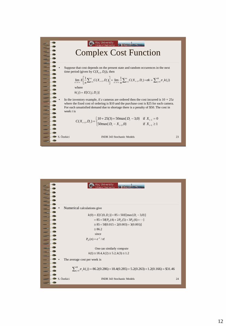
Average Cost
• Suppose that the Markov chain incurs the cost C(i) everytime state i is visited, then
the average cost per time is
• Suppose that there is a storage cost charged at the end of each week for items held in
stock so that C(0) = 0, C(1) = 2, C(2) = 8 and C(3) = 18, then the average storage
cost per week is
++
M
j j
n
t tn
n
t tn
jCCXCn
XCn
E011
)()(1
lim)(1
lim
662.5)18(166.0)8(263.0)2(285.0)0(286.0)(1
lim1
+++ +
n
t tn
XCn
12
S. Özekici INDR 343 Stochastic Models 23
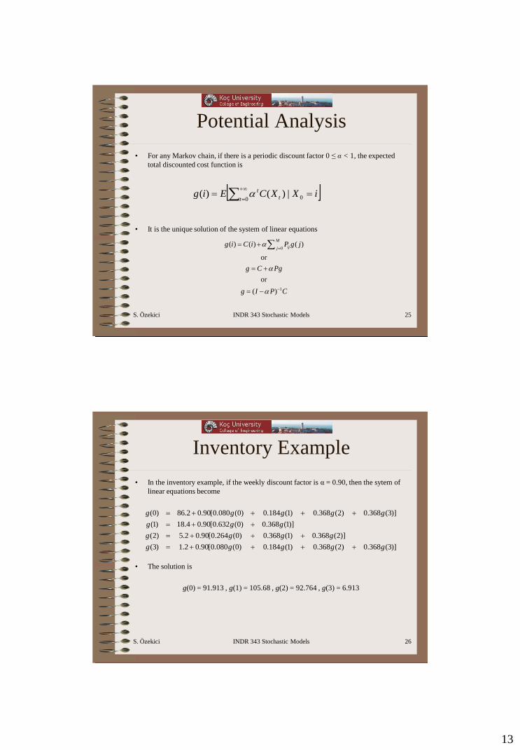
Complex Cost Function
• Suppose that cost depends on the present state and random occurences in the next
time period (given by C(Xt-1, Dt)), then
• In the inventory example, if z cameras are ordered then the cost incurred is 10 + 25z
where the fixed cost of ordering is $10 and the purchase cost is $25 for each camera.
For each unsatisfied demand due to shortage there is a penalty of $50. The cost in
week t is
)],([)(
where
)(),(1
lim),(1
lim01 11 1
t
M
j j
n
t ttn
n
t ttn
DjCEjk
jkkDXCn
DXCn
E
+ +
++
1 if}0,50max{
0 if}0,350max{25(3)10),(
11
1
1
ttt
tt
ttXXD
XDDXC
S. Özekici INDR 343 Stochastic Models 24
• Numerical calculations give
• The average cost per week is
2.1)3(,2.5)2(,4.18)1(
computesimilarly can One
!/)(
since
2.86
)]001.0(3)003.0(2015.0[5085
])6(3)5(2)4([5085
}]0,3{max[5085)],0([)0(
1
+++
++++
+
kkk
nenP
PPP
DEDCEk
D
DDD
tt
46.31$)166.0(2.1)263.0(2.5)285.0(4.18)286.0(2.86)(0
+++
M
j j jk
13
S. Özekici INDR 343 Stochastic Models 25
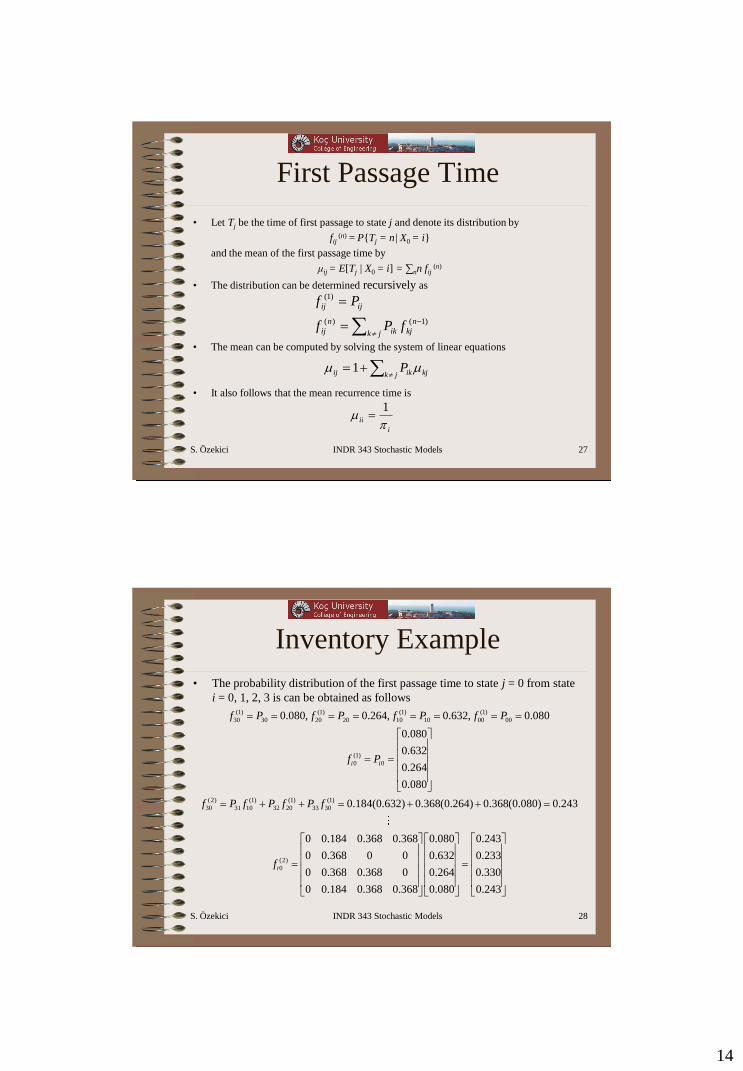
Potential Analysis
• For any Markov chain, if there is a periodic discount factor 0 ≤ α < 1, the expected
total discounted cost function is
• It is the unique solution of the system of linear equations
+
0 0|)()(t t
t iXXCEig
0
1
( ) ( ) ( )
or
or
( )
M
ijjg i C i P g j
g C Pg
g I P C
+
+
S. Özekici INDR 343 Stochastic Models 26
Inventory Example
• In the inventory example, if the weekly discount factor is α = 0.90, then the sytem of
linear equations become
• The solution is
g(0) = 91.913 , g(1) = 105.68 , g(2) = 92.764 , g(3) = 6.913
)]3(368.0)2(368.0)1(184.0)0(080.0[90.02.1)3(
)]2(368.0)1(368.0)0(264.0[90.02.5)2(
)]1(368.0)0(632.0[90.04.18)1(
)]3(368.0)2(368.0)1(184.0)0(080.0[90.02.86)0(
ggggg
gggg
ggg
ggggg
++++
+++
++
++++
14
S. Özekici INDR 343 Stochastic Models 27
First Passage Time
• Let Tj be the time of first passage to state j and denote its distribution by
fij (n) = P{Tj = n| X0 = i}
and the mean of the first passage time by
μij = E[Tj | X0 = i] = ∑nn fij (n)
• The distribution can be determined recursively as
• The mean can be computed by solving the system of linear equations
• It also follows that the mean recurrence time is
jk
n
kjik
n
ij
ijij
fPf
Pf
)1()(
)1(
+
jk kjikij P 1
i
ii
1
S. Özekici INDR 343 Stochastic Models 28
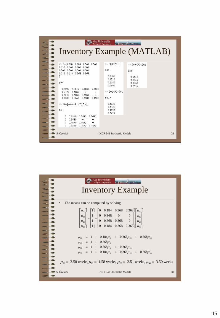
Inventory Example
• The probability distribution of the first passage time to state j = 0 from state
i = 0, 1, 2, 3 is can be obtained as follows
(1) (1) (1) (1)
30 30 20 20 10 10 00 00
(1)
0 0
(2) (1) (1) (1)
30 31 10 32 20 33 30
(2)
0
0.080, 0.264, 0.632, 0.080
0.080
0.632
0.264
0.080
0.184(0.632) 0.368(0.264) 0.368(0.080) 0.243
0
i i
i
f P f P f P f P
f P
f P f P f P f
f
+ + + +
0.184 0.368 0.368 0.080 0.243
0 0.368 0 0 0.632 0.233
0 0.368 0.368 0 0.264 0.330
0 0.184 0.368 0.368 0.080 0.243
15
S. Özekici INDR 343 Stochastic Models 29
Inventory Example (MATLAB)
S. Özekici INDR 343 Stochastic Models 30
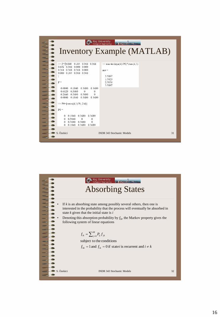
Inventory Example
00 10 20 30
10 10
20 10 20
30 10 20 30
1 0.184 0.368 0.368
1 0.368
1 0.368 0.368
1 0.184 0.368 0.368
+ + +
+
+ +
+ + +
00 10 20 30 3.50 weeks, 1.58 weeks, 2.51 weeks, 3.50 weeks
• The means can be computed by solving
00 00
10 10
20 20
30 30
1 0 0.184 0.368 0.368
1 0 0.368 0 0
1 0 0.368 0.368 0
1 0 0.184 0.368 0.368
+
16
S. Özekici INDR 343 Stochastic Models 31
Inventory Example (MATLAB)
S. Özekici INDR 343 Stochastic Models 32
Absorbing States
• If k is an absorbing state among possibly several others, then one is
interested in the probability that the process will eventually be absorbed in
state k given that the initial state is i
• Denoting this absorption probability by fik, the Markov property gives the
following system of linear equations
kiiff
fPf
ikkk
M
j jkijik
andrecurrent is state if 0 and 1
conditions thesubject to
0
17
S. Özekici INDR 343 Stochastic Models 33
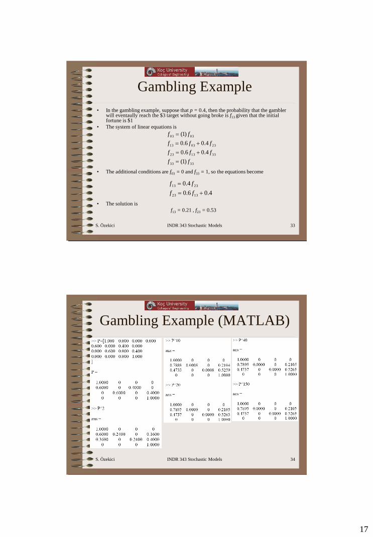
Gambling Example
• In the gambling example, suppose that p = 0.4, then the probability that the gambler will eventaully reach the $3 target without going broke is f13 given that the initial fortune is $1
• The system of linear equations is
• The additional conditions are f03 = 0 and f33 = 1, so the equations become
• The solution is
f13 = 0.21 , f23 = 0.53
3333
331323
230313
0303
)1(
4.06.0
4.06.0
)1(
ff
fff
fff
ff
+
+
4.06.0
4.0
1323
2313
+
ff
ff
S. Özekici INDR 343 Stochastic Models 34
Gambling Example (MATLAB)
18
S. Özekici INDR 343 Stochastic Models 35
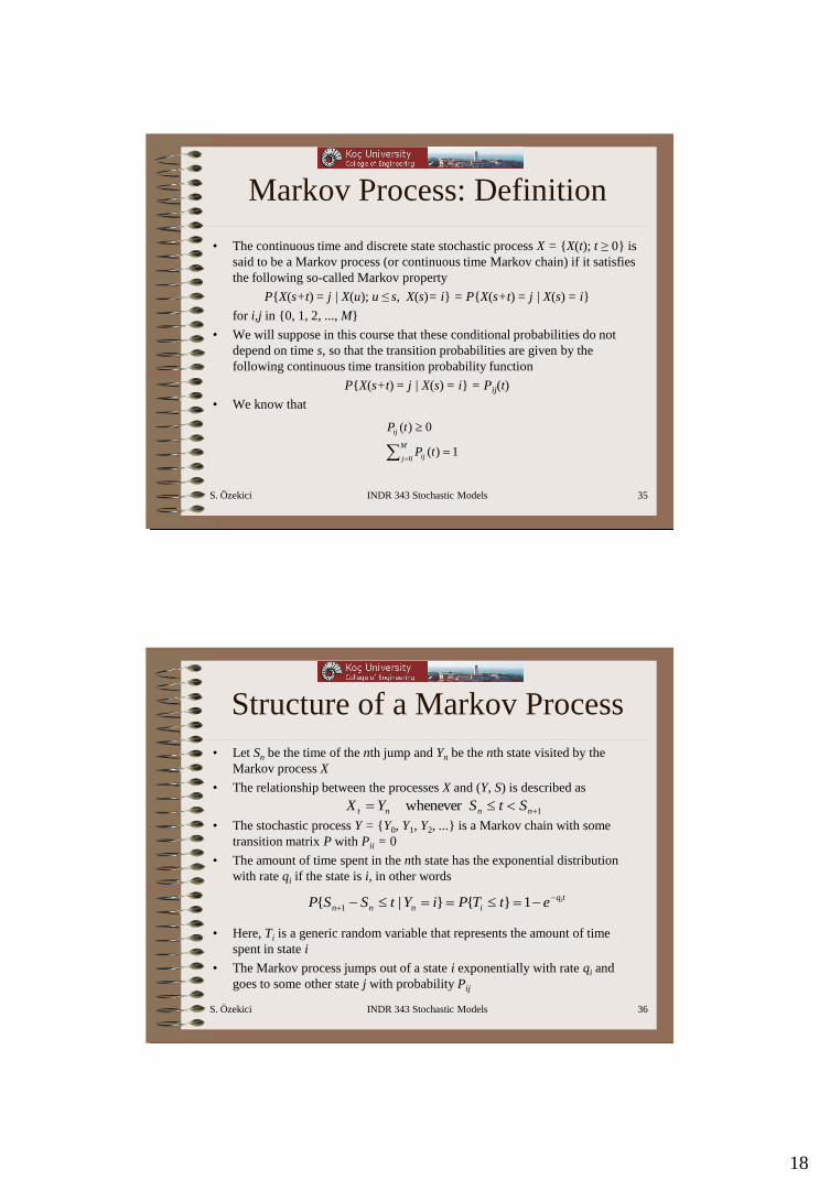
Markov Process: Definition
• The continuous time and discrete state stochastic process X = {X(t); t ≥ 0} is
said to be a Markov process (or continuous time Markov chain) if it satisfies
the following so-called Markov property
P{X(s+t) = j | X(u); u ≤ s, X(s)= i} = P{X(s+t) = j | X(s) = i}
for i,j in {0, 1, 2, ..., M}
• We will suppose in this course that these conditional probabilities do not
depend on time s, so that the transition probabilities are given by the
following continuous time transition probability function
P{X(s+t) = j | X(s) = i} = Pij(t)
• We know that
1)(
0)(
0
M
j ij
ij
tP
tP
S. Özekici INDR 343 Stochastic Models 36
Structure of a Markov Process
• Let Sn be the time of the nth jump and Yn be the nth state visited by the
Markov process X
• The relationship between the processes X and (Y, S) is described as
• The stochastic process Y = {Y0, Y1, Y2, ...} is a Markov chain with some
transition matrix P with Pii = 0
• The amount of time spent in the nth state has the exponential distribution
with rate qi if the state is i, in other words
• Here, Ti is a generic random variable that represents the amount of time
spent in state i
• The Markov process jumps out of a state i exponentially with rate qi and
goes to some other state j with probability Pij
1er whenev + nnnt StSYX
tq
innnietTPiYtSSP
+ 1}{}|{ 1
19
S. Özekici INDR 343 Stochastic Models 37
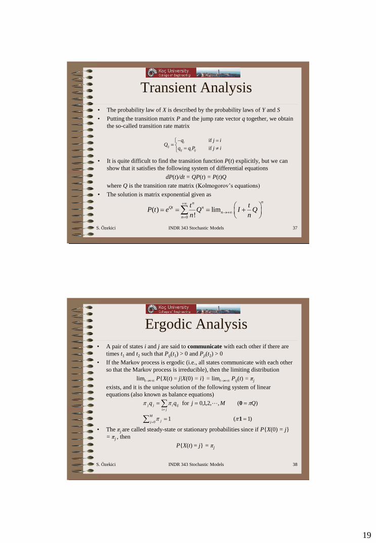
Transient Analysis
• The probability law of X is described by the probability laws of Y and S
• Putting the transition matrix P and the jump rate vector q together, we obtain
the so-called transition rate matrix
• It is quite difficult to find the transition function P(t) explicitly, but we can
show that it satisfies the following system of differential equations
dP(t)/dt = QP(t) = P(t)Q
where Q is the transition rate matrix (Kolmogorov’s equations)
• The solution is matrix exponential given as
if
if
i
ij
ij i ij
q j iQ
q q P j i
0
( ) lim!
nnQt n
n
n
t tP t e Q I Q
n n
+
+
+
S. Özekici INDR 343 Stochastic Models 38
Ergodic Analysis
• A pair of states i and j are said to communicate with each other if there are
times t1 and t2 such that Pij(t1) > 0 and Pji(t2) > 0
• If the Markov process is ergodic (i.e., all states communicate with each other
so that the Markov process is irreducible), then the limiting distribution
limt+∞ P{X(t) = j|X(0) = i} = limt+∞ Pij(t) = πj
exists, and it is the unique solution of the following system of linear
equations (also known as balance equations)
• The πj are called steady-state or stationary probabilities since if P{X(0) = j}
= πj , then
P{X(t) = j} = πj
)1( 1
)( ,,2,1,0for
0
1
0
M
j j
ji
ijijj QMjqq
20
S. Özekici INDR 343 Stochastic Models 39
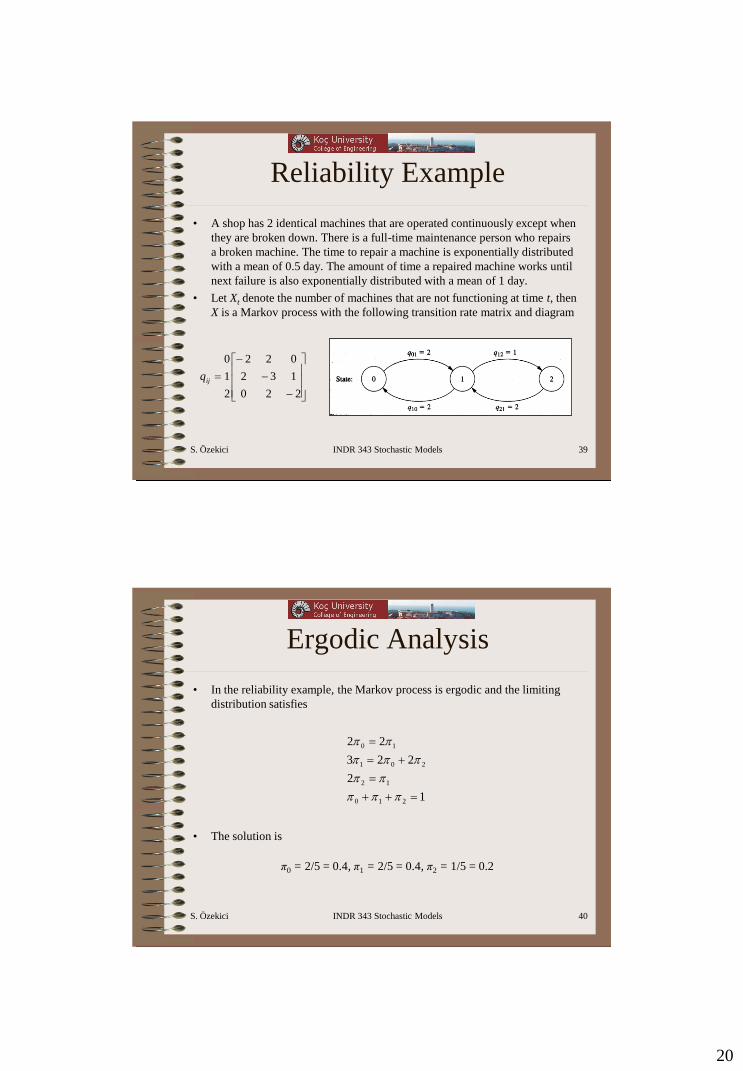
Reliability Example
• A shop has 2 identical machines that are operated continuously except when
they are broken down. There is a full-time maintenance person who repairs
a broken machine. The time to repair a machine is exponentially distributed
with a mean of 0.5 day. The amount of time a repaired machine works until
next failure is also exponentially distributed with a mean of 1 day.
• Let Xt denote the number of machines that are not functioning at time t, then
X is a Markov process with the following transition rate matrix and diagram
220
132
022
2
1
0
ijq
S. Özekici INDR 343 Stochastic Models 40
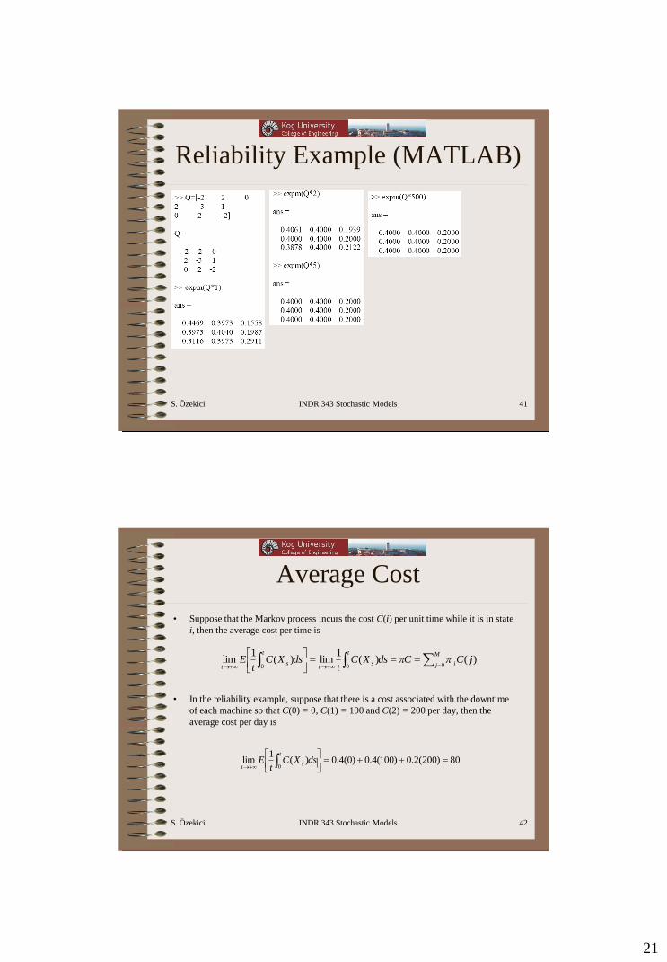
Ergodic Analysis
• In the reliability example, the Markov process is ergodic and the limiting
distribution satisfies
• The solution is
π0 = 2/5 = 0.4, π1 = 2/5 = 0.4, π2 = 1/5 = 0.2
1
2
223
22
210
12
201
10
++
+
21
S. Özekici INDR 343 Stochastic Models 41
Reliability Example (MATLAB)
S. Özekici INDR 343 Stochastic Models 42
Average Cost
• Suppose that the Markov process incurs the cost C(i) per unit time while it is in state
i, then the average cost per time is
• In the reliability example, suppose that there is a cost associated with the downtime
of each machine so that C(0) = 0, C(1) = 100 and C(2) = 200 per day, then the
average cost per day is
++
M
j j
t
st
t
st
jCCdsXCt
dsXCt
E000
)()(1
lim)(1
lim
80)200(2.0)100(4.0)0(4.0)(1
lim0
++
+
dsXCt
Et
st
22
S. Özekici INDR 343 Stochastic Models 43
Potential Analysis
• For any Markov process, if there is a continuous discount factor α > 0, the
expected total discounted cost function is
• It is the unique solution of the system of linear equations
+ iXdsXCeEig s
s
00
|)()(
0
1
( ) ( ) ( )
or
or
( )
M
ijjg i C i q g j
g C Qg
g I Q C
+
+
S. Özekici INDR 343 Stochastic Models 44
Reliability Example
• In the reliability example, if the discount factor is α = 0.95, then the sytem of linear
equations become
• The solution is
g(0) = 59.371 , g(1) = 87.572 , g(2) = 127.17
)2(2)1(2200)2(95.0
)2()1(3)0(2100)1(95.0
)1(2)0(20)0(95.0
ggg
gggg
ggg
++
++
+
23
S. Özekici INDR 343 Stochastic Models 45
Homework 1 & 2
• Homework 1
– 29.2-2
– 29.2-3
– 29.3-2
– 29.4-2
– 29.4-5
• Review Exercises 1
– 29.4-3
– 29.5-5
– 29.6-1
– 29.7-1
– 29.7-2
• Homework 2
– 29.5-4
– 29.5-9
– 29.6-5
– 29.8-1
– 29.8-2