1

Network monitoring: detecting node failures

2

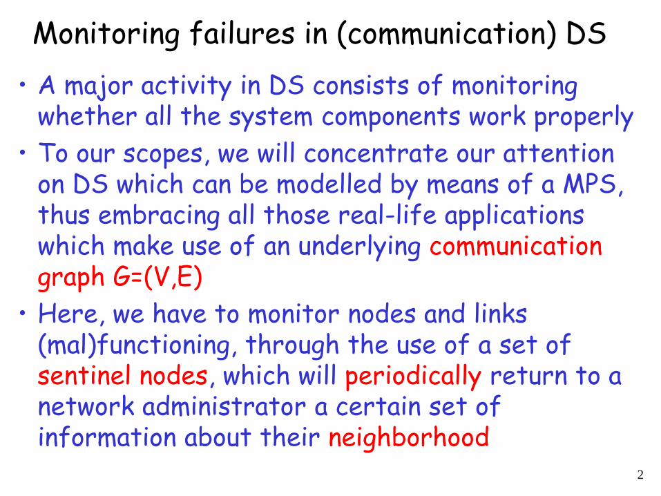
Monitoring failures in (communication) DS

• A major activity in DS consists of monitoring whether all the system components work properly

• To our scopes, we will concentrate our attention on DS which can be modelled by means of a MPS, thus embracing all those real-life applications which make use of an underlying communication graph G=(V,E)

• Here, we have to monitor nodes and links (mal)functioning, through the use of a set of sentinel nodes, which will periodically return to a network administrator a certain set of information about their neighborhood

Example: locating a burglar This could be your nice apartment

3

Problem: suppose that you want to protect it against intrusions, and that you decide to install an Intruder Detection System (IDS) guarding the apartment, based on video surveillance.

… and so you decide to put 2 cameras in rooms b and c (it is easy to see that in this way all the rooms are guarded)

Example: locating a burglar (2) Suppose now that you leave the apartment and a burglar enters in ; your IDS detects it and remotely inform you about that…

4

Question: can you call the police and tell them precisely in which room the burglar is located? This depends on the information returned by the IDS…

Example: locating a burglar (3) Luckily enough, you installed an IDS consisting of advanced cameras, each of which can return the name of the room from which the intrusion comes:

5

In this case, cameras in rooms b and c will both tell to you "room f", and so the burglar will be exactly located

Example: locating a burglar (4) On the other hand, assume that you had installed an IDS guarding the apartment consisting of basic cameras, which are only able to send an alarm bit after they detect an intrusion in a guarded room; so, both b and c reports an alarm bit…

6

…but now the question is: where is the burglar? Either in room b, c, or f??? The IDS does not work properly here, since we do not know in which room the burglar is!

Example: locating a burglar (5) However, if you had installed 4 basic cameras guarding the apartment as in the picture, the situation gets back to be safe:

7

Now cameras b and c send an alarm bit, but a and d do not, and so you can infer the burglar is in room f… can you see why?

Because each room has a distinct set of guarding cameras!

8

Transposition to network monitoring • While in the previous example, the IDS monitors the apartment for

threats from the outside, a network monitoring system (NMS) monitors the network for problems caused by crashed servers (nodes), or network connection disruptions (edges).

• A NMS has to monitor continuously the network, and has to report immediately a malfunctioning: in a MPS, this means that we need synchronicity among processors.

• In a NMS, the status of nodes and edges is monitored through the use of sentinel nodes, which periodically exchange messages with adjacent nodes (for instance, a reciprocal status request every k rounds), and then report some kind of information to the network administrator.

• Which type of information a sentinel node is able to report to the network administrator? This depends on the underlying network infrastructure, along with the monitoring software. For instance, in a wireless network, a sentinel node could not be able to precisely establish which of its neighbors is not replying to a ping, and so it can only return an alarm bit to the administrator!

Formalizing the node-monitoring problem

• Input: A graph G = (V,E) modeling a MPS, and a query model Q, namely a formal description of the entire process through which a sentinel node x reports its piece of information to the network administrator (i.e., (1) which nodes are queried by x, and (2) which type of information x can return to the system as a result of the queries);

• Goal: Compute a minimum-size subset of sentinel nodes SV allowing to monitor G with respect to the simultaneous failure of at most k nodes in G, i.e., such that the composition of the information reported by the nodes in S to the network administrator is sufficient to identify the precise set of crashed nodes, for any such set of size at most k.

10

Again on the query model

• In the burglar example, the query model is the following: 1. each sentinel (i.e., camera) monitors its adjacent nodes only;

2. in the first scenario (advanced cameras) a sentinel node returns the name of an adjacent affected node, while in the second case (basic cameras) it just returns the information that an adjacent node has been affected

• This is exactly what the definition of a query model is about: the set of information that a sentinel node x is able to return.

• Observe that the larger is the set of returned information, the stronger is the query model, and the sparser is the set of sentinels that we need to monitor the graph!

11

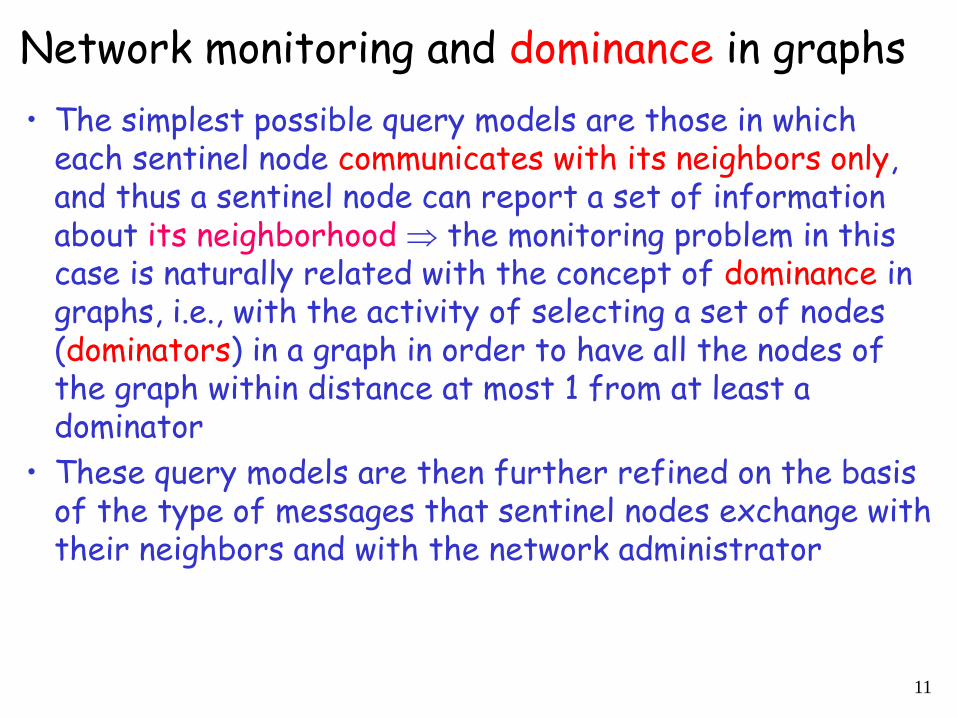
Network monitoring and dominance in graphs

• The simplest possible query models are those in which each sentinel node communicates with its neighbors only, and thus a sentinel node can report a set of information about its neighborhood the monitoring problem in this case is naturally related with the concept of dominance in graphs, i.e., with the activity of selecting a set of nodes (dominators) in a graph in order to have all the nodes of the graph within distance at most 1 from at least a dominator

• These query models are then further refined on the basis of the type of messages that sentinel nodes exchange with their neighbors and with the network administrator

12

Dominating Set

Given a graph G=(V,E), a dominating set of G is a set of nodes D such that every node of G is at distance at most 1 from D

|D|=4 x

y z

x dominates {x,y,z}

13

Minimum Dominating Set (MDS):

This is a dominating set of minimum size

|D*|=3 x

y z

a b

c

d

e

f

g

14

In a query model in which a sentinel node: 1. Sends a ping to each adjacent node and waits for a reply; 2. Sends to the network administrator the id of the set of

adjacent nodes which did not reply;

a MDS D* of a graph G=(V,E) defines a minimum-size set of processors which can monitor the correct functioning of all the nodes in V\D*, since every node in G is pinged by at least one node in D* (notice that if a node x in D* fails, the network administrator is not able to understand whether –besides x- some of the nodes dominated by x have failed or not; thus, an MDS is not enough to monitor the entire graph, but only the nodes in V\D*. On the other hand, if we are guaranteed that at most a single node in G can fail, then a MDS is enough to monitor the entire graph!)

Network monitoring and MDS

15

A special type of Dominating Set:

the Identifying Code (IC) This is a dominating set D in which every node v is dominated by a distinct set of nodes in D (this is called the identifying set of v)

x

y z

a b

c

d

e

g {a,x}

{a}

f

d

{a,c} {c,d,g}

{d,g}

{c,x,d}

{c}

{x}

{d} {g}

A Minimum IC (MIC) is an IC of smallest cardinality.

16

In a query model in which a sentinel node: 1. Sends a ping to each adjacent node and waits for a reply; 2. Sends to the network administrator an alarm bit (0 if all the

adjacent replied, 1 otherwise);

a MIC C* of a graph G=(V,E) defines a minimum-size set of processors which can monitor the failure of at most one node in V\C*, since every node in G is pinged by a distinct set of nodes in C* (notice that if a node x in C* fails, the network administrator is not able to understand whether –besides x- some of the nodes dominated by x have failed or not; so again, if we are guaranteed that at most a single node in G can fail, then a MIC is enough to monitor the entire graph!)

Network monitoring and MIC

17

Our problems • We will study the monitoring problem for single node

failures (i.e., node crashes) w.r.t. the two following two query models: 1. Sentinels are able to return the id of the adjacent failed node

we will search a MDS of the network (MDS problem) 2. Sentinels are only able to return an alarm bit about the

neighborhood (i.e., a warning that an adjacent node has failed) we will search a MIC of the network (MIC problem)

• Main questions: Are MDS and MIC problems easy or NP-hard? If so, can we provide efficient (distributed) approximation algorithms to solve them?

• We will show that MDS and MIC problems are NP-hard, and that they are both not approximable within o(ln n); we will also provide an Θ(ln n)-approximation distributed algorithm for MDS and MIC (only a sketch)

Reminder: being NP-hard • A decision problem P is NP-hard iff one can reduce in

polynomial time any NP-complete problem P’ to it, i.e., there exists a polynomial-time algorithm that maps an instance of P’ to an instance of P, and such that the YES-instances of P’ will be mapped to the YES-instances of P, and vice-versa (this is a.k.a. Karp reduction, denoted by P’ ≤K P)

• Of course, if we could solve an NP-hard problem in polynomial time, then P=NP

• Notice that MDS and MIC are optimization problems, since we search for solutions of minimum size, and so they are not encompassed by the above NP-hardness definition

• However, it is easy to provide a decision version of an optimization problem, without affecting its intrinsic complexity: it suffices to add a threshold value to the input, and then asking whether a solution either above or below that threshold does actually exist In the following, we will assume that the class NP-hard contains both decision and optimization problems

The class NP-hard: a picture

19

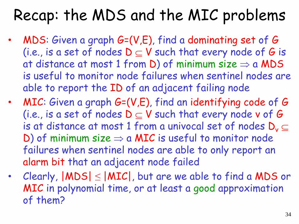
Recap: the MDS and the MIC problems

• MDS: Given a graph G=(V,E), find a dominating set of G (i.e., is a set of nodes D V such that every node of G is at distance at most 1 from D) of minimum size a MDS is useful to monitor node failures when sentinel nodes are able to report the ID of an adjacent failing node

• MIC: Given a graph G=(V,E), find an identifying code of G (i.e., is a set of nodes D V such that every node v of G is at distance at most 1 from a univocal set of nodes Dv D) of minimum size a MIC is useful to monitor node failures when sentinel nodes are able to only report an alarm bit that an adjacent node failed

• Clearly, |MDS| ≤ |MIC|, but are we able to find a MDS or MIC in polynomial time, or at least a good approximation of them?

34

Reminder: optimization problems and approximability

• An optimization problem A is a quadruple (I, F, c, g), where • I is a set of instances; • given an instance x ∈ I, F(x) is the set of feasible solutions; • given a feasible solution y ∈ F(x), c(y) denotes the cost of y, which is

usually a positive real; • g is the goal function, and is either min or max. • The goal is then to find for some instance x an optimal solution, that is, a

feasible solution y with c(y) = g {c(y') | y' ∈ F(x)}.

• For NP-hard optimization problems, unfortunately we do not know polynomial-time solving algorithms, thus we resort to approximation algorithms: Given a minimization (resp., maximization) problem A, let OPTA(x) denote the cost of an optimal solution for A w.r.t. the instance x; then, we say that A is ρ-approximable, with ρ≥1 (resp., ρ≤1), if there exists a polynomial-time algorithm for A which for any instance x ∈ I returns a feasible solution whose measure is at most (resp., at least) ρ∙OPTA(x).

• Moreover, we say that A is ρ-inapproximable, if under some reasonable assumptions (typically, PNP), A is not ρ-approximable

(In)Approximability of MDS

• Unfortunately, MDS is NP-hard, and even worse, it cannot be approximated (in polynomial time) within (1-ε) ln n, for any ε > 0, unless NP DTIME(nlog log n) (i.e., unless NP has deterministic algorithms operating in slightly super-polynomial time – this is just a bit more believable to happen than P=NP).

• On the positive side, there exists an easy greedy heuristic for MDS providing a (tight) Θ(ln n) approximation ratio.

36

37

Centralized MDS Greedy Algorithm (1/4)

Greedy Algorithm (GA): For any node v of the given graph G, define its span to be the number of non-dominated nodes in {v} U N(v). Then, start with empty dominating set D, and at each step add to D node v with maximum span, until all nodes are dominated.

Theorem: The GA is H(+1)-approximating, where

is the degree of G, and H(k) = 1+1/2+1/3+…+1/k ≤ 1+ln k, i.e., the GA is (1+ln (+1))-approximating, or (1+ln n)-approximating.

38

Centralized MDS Greedy Algorithm (2/4)

Proof: We prove the theorem by using amortized analysis. We call black the nodes in D, grey the nodes which are dominated (neighbors of nodes in D), and white all the non-dominated nodes. Each time we choose a new node of the dominating set (each greedy step), we have a cost of 1, (since one node is added to the solution), but instead of assigning the whole cost to the node we have chosen, we distribute the cost equally among all newly dominated nodes.

Now, assume that we know a MDS D*. By definition, to each node which is not in D*, we can assign a neighbor from D*. By assigning each node to exactly one node of D*, the graph is decomposed into stars, each having a dominator (node in D*) as center, and non-dominators as leaves. Clearly, the cost of a MDS is 1 for each such star, or, in other words, each node of a star of k+1 nodes centered at vD* and of degree k (i.e., with k leaves) will cost 1/(k+1). But what the cost of such a star will be in the solution found by the GA?

39

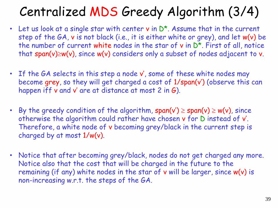
Centralized MDS Greedy Algorithm (3/4) • Let us look at a single star with center v in D*. Assume that in the current

step of the GA, v is not black (i.e., it is either white or grey), and let w(v) be the number of current white nodes in the star of v in D*. First of all, notice that span(v)w(v), since w(v) considers only a subset of nodes adjacent to v.

• If the GA selects in this step a node v’, some of these white nodes may become grey, so they will get charged a cost of 1/span(v’) (observe this can happen iff v and v’ are at distance at most 2 in G).

• By the greedy condition of the algorithm, span(v’) span(v) w(v), since otherwise the algorithm could rather have chosen v for D instead of v’. Therefore, a white node of v becoming grey/black in the current step is charged by at most 1/w(v).

• Notice that after becoming grey/black, nodes do not get charged any more. Notice also that the cost that will be charged in the future to the remaining (if any) white nodes in the star of v will be larger, since w(v) is non-increasing w.r.t. the steps of the GA.

40

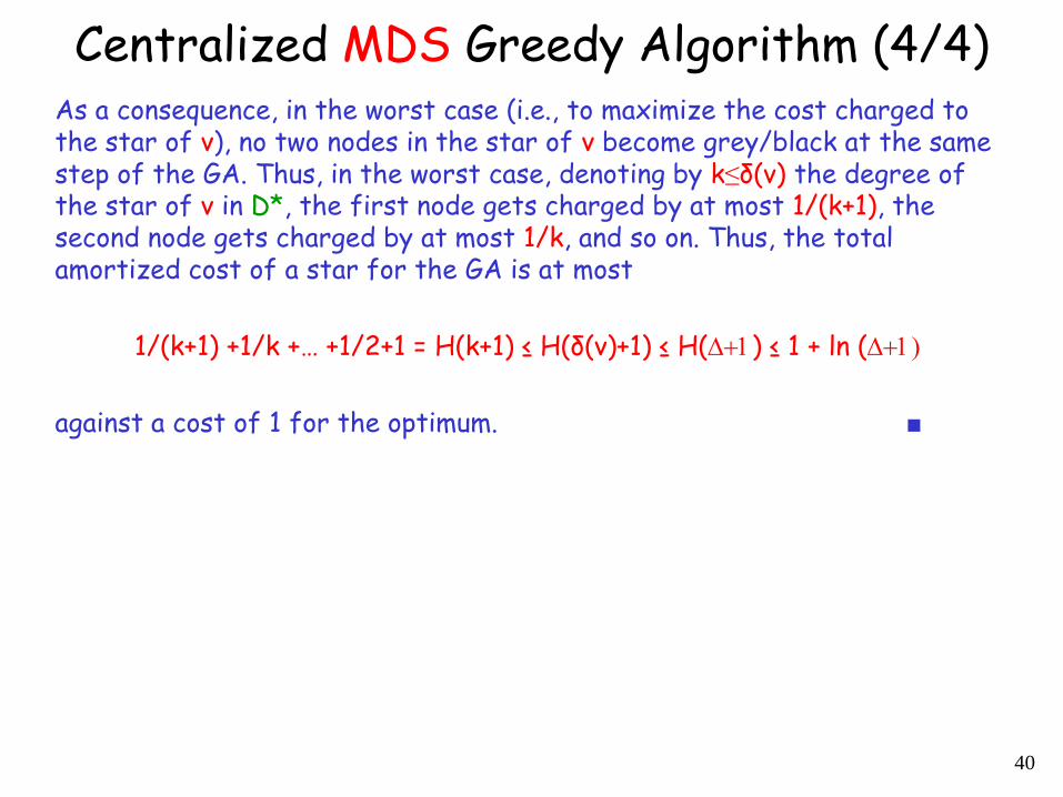
Centralized MDS Greedy Algorithm (4/4) As a consequence, in the worst case (i.e., to maximize the cost charged to the star of v), no two nodes in the star of v become grey/black at the same step of the GA. Thus, in the worst case, denoting by k≤δ(v) the degree of the star of v in D*, the first node gets charged by at most 1/(k+1), the second node gets charged by at most 1/k, and so on. Thus, the total amortized cost of a star for the GA is at most

1/(k+1) +1/k +… +1/2+1 = H(k+1) ≤ H(δ(v)+1) ≤ H(+1) ≤ 1 + ln (+1)

against a cost of 1 for the optimum. ■

41

Distributing (synchronously) the GA (1/2)

• Synchronous, non-anonymous, uniform MPS

• Proceed in phases, initially no node is in D

• Each phase has 3 steps: 1. each node calculates its current span, by

testing adjacent nodes (2 rounds);

2. each node sends (span, ID) to all nodes within distance 2 (2 rounds);

3. each node joins the dominating set D iff its (span, ID) is lexicographically higher than all others within distance 2 (1 round to notify neighbors)

42

Distributing (synchronously) the GA (2/2) • It can be easily proven that the distributed algorithm has the same

approximation ratio as the greedy algorithm: indeed, the analysis of the GA only involves nodes which are at distance at most 2 in G, as we have observed in the proof, which is exactly the tested neighborhood of the distributed algorithm

• However, the algorithm can be quite slow, since it can take O(|D|) phases to terminate, where D is the returned dominated set. Look for instance at the following caterpillar graph (path of decreasing degrees) of n nodes:

Nodes along the "backbone" (of length (n)) add themselves to D

sequentially from left to right (n) phases (and rounds) are needed!

Via randomization, the greedy algorithm can be modified so as to terminate w.h.p. in O(log log n) rounds, with an expected O(log )-approximation ratio.

Special cases • If the graph has maximum degree Δ=O(1), then the

greedy approximation algorithm finds an O(log Δ)=O(1)-approximation of a MDS.

• For special (but still prominent, from an application point of view) cases, such as unit disk graphs (UDG) and planar graphs (PG), the problem admits a (centralized) polynomial-time approximation scheme (PTAS), where: 1. A UDG is the intersection graph of a set of unit circles in the

Euclidean plane; they are often used to model wireless networks.

2. A PG is a graph that can be drawn in such a way that no edges “cross” each other; they are often used to model transportation networks, but also communication networks.

3. A PTAS is an algorithm which takes an instance of a minimization (resp., maximization) problem, and a parameter ε > 0, and in polynomial time (for fixed ε, e.g., in time O(n1/ε)), produces a solution that is within a factor 1+ε (resp., 1–ε) from the optimal.

43

A unit disk graph

44

Some planar graphs

45

(In)approximability of MIC

• Concerning the MIC problem, the situation is very similar to MDS.

• More precisely, MIC is NP-hard and cannot be approximated within (1-ε) ln n, for any ε > 0, unless NP DTIME(nlog log n).

• On the positive side, there exists a sequential (1+ln n)-approximation algorithm for MIC.

• Moreover, the distributed GA for the MDS problem can be easily modified to solve the MIC problem in a distributed setting (it will essentially explore the 3-neighborood of a node instead of its 2-neighborood), and it will run in O(|IC|), where IC is the returned identifying code. 46

Assignment 1. Provide a message complexity analysis of the

distributed GA for the MDS problem

2. Run the greedy algorithm for the MDS problem on the following graph (the optimum is given by red nodes), and compute the apx ratio

47