network and sensor management for multiple sensor emitter location
TRANSCRIPT

NETWORK AND SENSOR MANAGEMENT
FOR MULTIPLE SENSOR EMITTER
LOCATION SYSTEM
BY
XI HU
BEng, Liaoning University, China, 1998 MEng, Beijing Jiaotong University, China, 2001
MS, Binghamton University, Binghamton, New York, 2007
DISSERTATION
Submitted in partial fulfillment of the requirements for the degree of Doctor of Philosophy in Electrical Engineering
in the Graduate School of Binghamton University
State University of New York 2008

copyright by
Xi Hu
2008

iii
Accepted in partial fulfillment of the requirements for the degree of Doctor of Philosophy in Electrical Engineering
in the Graduate School of Binghamton University
State University of New York 2008
October 8, 2008
Mark L. Fowler, Department of Electrical and Computer Engineering, Binghamton University
Eva Wu, Department of Electrical and Computer Engineering, Binghamton University
Xiaohua Li, Department Electrical and Computer Engineering, Binghamton University
iv
ABSTRACT
In order for estimating the location of a passive emitter, signal data must be collected
at a multitude of sensors and the sensors must cooperate to achieve the task. Our goal is
to achieve network-wide optimization over a large number of simultaneously deployed
sensors to enable more efficient and effective cooperation within the network of sensors.
This dissertation covers the following aspects: i) The emitter location estimation
accuracy is related with many items, giving an overall review of how the measurements
quality (such as the accuracies of TDOA and FDOA) and sensors’ navigation data (such
as position and velocity) will affect the estimation errors, and developing the relationship
among those aspects; (ii) Since the accuracy of parameter estimation is related with the
signal model, exploiting the importance of deciding the signal model used in location
estimation problem and giving out the results of different models; (iii) To save the system
energy and reduce computation latency, developing various methods to select and pair a
subset of sensors to satisfy the system requirements; (iv) Based on the relationship
between estimation accuracy and sensors’ navigation data, discussing the probability of
computing the next optimal state; (v) Since sensors’ navigation data along with
uncertainty, exploiting the sensors’ navigation data errors effects on least square
estimation and giving solution to mitigate these errors. The results of this dissertation will
provide a systematic means for addressing network management and sensor management
issues across the spectrum of sensor network.

v
ACKNOWLEDGEMENTS
I wish to acknowledge the guidance and advising of my advisor, Professor Mark L.
Fowler. I appreciate everything that he has done in helping my dissertation along, and for
offering support and encouraging during my studying. I would also like to thank
Professor Eva Wu for her helpful discussion and guidance concerning my research.
Additionally, I thank two committee members Professor Xiaohua Li and Professor
Harold W. Lewis for their service on my dissertation committee and their reviewing my
dissertation.
I would like to thank my parents for their never ending love. Especially, I appreciate
my husband for all he has done to me; he is always supportive of me. Without any of you,
this dissertation would never have been possible.
Also thanks to my friends at Binghamton University, they make my life here
wonderful.

vi
CHAPTERS
1 Introduction......................................................................................................... 1
2 Parameter Estimation......................................................................................... 5
2.1 Signal Model.................................................................................................. 5
2.2 Cramer-Rao Lower Bound and Fisher Information....................................... 8
2.3 Maximum Likelihood Estimator.................................................................. 11
2.4 Least Square Estimator ................................................................................ 13
3 TDOA/FDOA Localization-Known and New Foundations .......................... 17
3.1 Overview of TDOA/FDOA Location .......................................................... 18
3.1.1 Doppler Shift and Time Delay .........................................................................................18
3.1.2 First stage: TDOA/FDOA Estimation ..............................................................................21
3.1.3 Second Stage: Emitter Location Estimation.....................................................................23
3.2 Importance of Signal Model ....................................................................... 25
3.2.1 Common and Uncommon Aspects of Acoustic and Electromagnetic Signals .................26
3.2.2 Fisher Information for the Two Scenarios........................................................................28
3.2.3 Maximum Likelihood Estimator for the Two Scenarios ..................................................31
3.3 Characterizing TDOA/FDOA Performance for RF Emitters ...................... 33
3.3.1 Evaluating the FIM of One Pair .......................................................................................33
3.3.2 Evaluating the FIM of Two Pairs Sharing One Sensor.....................................................35
3.4 Characterizing Location Performance for RF Emitters ............................... 37
3.4.1 Emitter Location Accuracy as a Function of TDOAs and Sensor States Measurements..39
3.4.2 Emitter Location Accuracy as a Function of FDOA and Sensor States Measurements ...42
3.5 Appendix 3A-Convergence of Gauss-Newton Least Square Method ......... 45

vii
4 Network Management---FIM Based Sensor Selection and Pairing ............. 48
4.1 Optimal Criterion......................................................................................... 49
4.1.1 Covariance Matrix and Error Ellipsoid ............................................................................50
4.1.2 Criterion Selection ...........................................................................................................52
4.2 Diversity of Sensor Selection and Pairing ................................................... 55
4.2.1 Network Types .................................................................................................................55
4.2.2 Two Pairing Scenarios......................................................................................................56
4.3 Sensor Selection and Pairing Strategies....................................................... 57
4.3.1 Pre-Paired Sensors ...........................................................................................................57
4.3.2 Free Sensors .....................................................................................................................61
4.3.3 Trade Off Between Non-Sharing and Sharing Methods...................................................71
Appendix-4A an Example of Branch and Bound Method Used in Sensor Pairing 72
5 Sensors’ Navigation Data Error Effects and Mitigation............................... 77
5.1 Least-Squares Estimation Error Model........................................................ 77
5.2 CRLB Revisit............................................................................................... 81
5.3 Updated Weighted Matrix............................................................................ 84
5.4 Estimation Accuracy with Local State Error ............................................... 84
5.4.1 TDOA ..............................................................................................................................85
5.4.2 FDOA...............................................................................................................................86
5.5 Appendix-5A Total Least Square Method for NAV Data Errors ................ 87
5A.1 Introduction of TLS ..............................................................................................................87
5A.2 TLS Performance for Emitter Location Estimation ..............................................................91
6 More Issues about Estimation Accuracy ........................................................ 94
6.1 Gaussian Maximum Likelihood Estimator .................................................. 94
6.1.1 CML and DML Estimators...............................................................................................95
6.1.2 DML TDOA/FDOA Estimates.......................................................................................100
viii
6.2 Next Optimal State..................................................................................... 103
6.2.1 Optimal Criterion ...........................................................................................................105
6.2.2 Minimize Trace of 1geo−J .................................................................................................106
6.2.3 Minimize Determinant of 1geo−J ......................................................................................108
6.3 Sensor Error Effects on Next Optimal State Solution ............................... 109
6.3.1 Uncertainty on Trace of geoJ ........................................................................................110
6.3.2 Uncertainty on Determinant of geoJ .............................................................................112
7 Conclusion and Future Work ........................................................................ 113
8 References........................................................................................................ 116

ix
LIST OF FIGURES
Figure 1 Likelihood function of unknown parameter evaluated on fixed measured
data.................................................................................................................................... 12
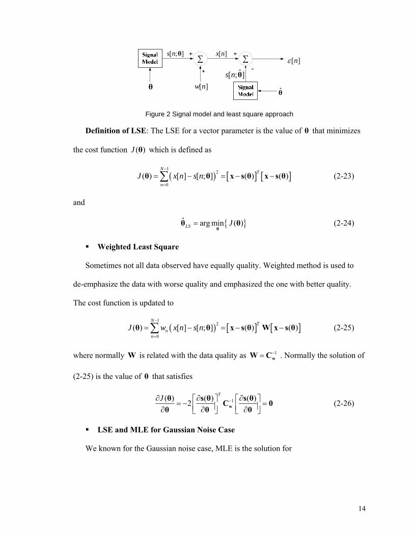
Figure 2 Signal model and least square approach....................................................... 14
Figure 3 Geometry for stationary source localization system. ................................... 21
Figure 4 Vectors used in TDOA/FDOA equations illustration for one pair................ 23
Figure 5 Three sensors and two pairs ......................................................................... 35
Figure 6 Randomness of the intersection of two TDOA hyperbolas .......................... 39
Figure 7 Fact orating edp into two parts .................................................................... 40
Figure 8 Angles illustration for FDOAs system ......................................................... 43
Figure 9 Error ellipse and coordinate axes in the ....................................................... 51
Figure 10 Three type of sensor networks.................................................................... 56
Figure 11 Layout of 10 pairs of sensor ....................................................................... 59
Figure 12 Simulation result for FIM-based sensor pairs selection w/o sharing. ........ 59
Figure 13 Sensor sets example.................................................................................... 60
Figure 14 For each group, renumber each pair ........................................................... 61
Figure 15 Simulation result for 14 free sensors selection and pairing........................ 63
Figure 16 An example of linearly independent and dependent pairs.......................... 65
Figure 17 An example of different choice of reference sensor ................................... 66
Figure 18 Example of sequence pairing and reference pairing................................... 70
Figure 19 Simulation result 10 free sensors selection and pairing with sensor sharing.
........................................................................................................................................... 71
Figure 20 First step tree structure ............................................................................... 73

x
Figure 21 Second step tree structure........................................................................... 74
Figure 22 Third step tree structure.............................................................................. 75
Figure 23 Simulation result for time consumption comparison between of 'branch and
bound’ method and enumerating method.......................................................................... 76
Figure 24 Centralized cross-correlation vs. de-centralize cross-correlation method.. 95

1
1 Introduction
Estimating the location of a passive emitter has been a research issue for decades ([6]-
[21]). The estimation procedure has two steps. First: estimate sensors’ received signal
parameters, such as arriving time, frequency, angle, phase, or the energy. Second: use the
parameters estimated in the first stage to estimate the emitter location. These sensors are
located at some vehicles or aircrafts, and the unmanned vehicles are becoming more and
more popular. In order for wireless sensor networks to exploit a signal, signal data must
be collected at a multitude of sensors and the sensors must cooperate to achieve the task.
Our general interest is in achieving network-wide optimization over a large number of
simultaneously deployed sensors to enable more efficient and effective cooperation
within the network of sensors. Fisher information can be used to assess the data quality
across multiple sensors to manage the network of sensors to optimize the location
accuracy subject to communication constraints. For emitter location it is well-known that
the geometry between sensors and the target plays a key role in determining the location
accuracy. Furthermore, the deployed sensors have different data quality. Given these
two factors, it is no trivial matter to do the network and sensor management as mentioned
above.
Whatever methods used to estimate the emitter location will come with the estimation
errors. The estimation accuracy is related with many aspects: the sensors’ received signal
data quality, the sensors’ positions and velocities, and the related geometrical properties
among sensors and emitter. For examples, [16] gives the “one-sigma-width” to
characterize the emitter location accuracy, which is based on only one signal parameter
measurement. But for TDOA/FDOA (time difference of arrival/frequency difference of

2
arrival) localization problem, we need at least two (for two dimensional system) signal
parameters measurements to locate the emitter. [8] links the conventional accuracy
measures to the moments and products of inertia of a mass configuration and gives some
special geometry examples. We exploit the relationship between the emitter location
accuracy and all other accuracies of relative measurements and geometrical aspects in
general cases. It gives an overview of how all these aspects will affect the final accuracy,
and the trade off among them.
For the given sensors network, it is desirable to use the complete set of sensor
resources to do the task. However, that will result in an excessive data computation and
communication in the network. And the main constraints of wireless sensor network are
the limited on-board energy and limited channel resources. Many approaches have been
proposed in the past to satisfy the network resource requirements, such as routing, sleep
modes, low-power electronics, etc. For examples: one data compression method was
proposed by Professor Fowler and Dr. Mo Chen in Dr. Mo Chen’s dissertation [23].
Sensor selection is one of the solutions to save system energy which is to select a subset
of sensors to achieve the requirement. Using the information theory to do the sensor
selection was proposed in [36][37]. A new method is proposed in this dissertation: Fisher
information based Sensor Selection and Pairing, which is more efficient and accurate.
Our work is to manage the given set of sensors to satisfy the emitter location accuracy
demanding. We propose various approaches to this problem and discuss trade-offs among
them. For examples: One method assumes that the sensors have pre-paired and share
their data between these pairs; sensor selection then consists of selecting pairs to optimize
performance while meeting constraints on number of pairs selected; Another method

3
consists of optimally determining pairings as well as selections of pairs with or without
sensor sharing.
To estimate the emitter location, we need some signal’s measured/estimated
parameters from sensors’ received data, and we also need the sensors’ navigation data,
such sensors’ positions and velocities. In practice, the positions and velocities of sensors
can not be known exactly. A closed form solution to take the receiver error into account
was given in [40], which uses two steps estimation methods to solve the problems. We
exploit an expression about how these navigation data will affect the estimation accuracy
and give out an error mitigation processing, which will play an important role in the
decrease of estimation deviation. Our method is more simple and with less assumptions
compare with others’ methods.
Also if we can maneuver the sensors, based on the current information we have about
the sensors and the data quality, we can decide the next optimal states of sensors
(sensors’ positions and velocities) within the next research sets. It is called the maneuver
of sensors or trajectory planning. We proposed the basic idea about the next optimal
states. And developing solutions for some sub-optimal problems.
The contributions of this dissertation include: i) Giving an overall review of how the
measurements quality (such as the accuracies of TDOA and FDOA) and sensors’
navigation data (such as position and velocity) will affect the estimation errors, and
developing the relationship among those aspects; (ii) Exploiting the importance of
deciding the signal model used in location estimation problem, and giving out the
different results for different models on Fisher information calculation, maximum

4
likelihood estimator and etc.; (iii) Developing various methods to select and pair a subset
of sensors to satisfy the system requirements, such as saving system energy and reduce
computation latency; (iv) Exploiting the sensors’ navigation data errors effects on
calculation Fisher information and least square estimation, and giving solution to mitigate
these errors. (v) Discussing the probability of computing the next optimal state, and
giving some results on sub-optimal problems; The results of this dissertation will provide
the engineer with a systematic means for addressing network management and sensor
management issues across the spectrum of sensor network.

5
2 Parameter Estimation
Emitter localization is to estimate the emitter location by some parameters of the
signal sent by the emitter. There are two stages parameter estimations: one is the signal
parameter estimation, the other one is the emitter location estimation. In this chapter we
introduce the basic concepts, properties and two estimation methods of parameter
estimation we used in this dissertation.
2.1 Signal Model
Parameter estimation is to estimate a parameter through some measured data, which
depend on the unknown parameter. Assume we measured N samples data as
{ }[0], [1], , [ 1]x x x N= −x , the parameter estimator can be written as
ˆ( ) ( [0], [1], , [ 1])g x x x Nθ = −x (2-1)
where g is the function we used to estimate the parameter θ .
To estimate the parameter of a signal, we need a signal model first, which specifies
the relationship between the unknown parameter and received data. The data received are
random because of the noise coming with it, so we can describe it by its probability
density function (PDF). There are two different scenarios related with the deterministic
property of the parameter. (1) If the parameter to be estimated is deterministic, then the
PDF of received signal is parameterized by the unknown parameter as ( ; )p θx . The
estimation is called classical estimation, which we chose in this dissertation. (2) The
other scenario is that the unknown parameter is a random variable and we have a prior
knowledge about it, which is ( )p θ . The parameter to be estimated is viewed as one

6
realization of the random variable θ . The joint PDF of measured data and unknown
parameter can be written as ( , ) ( | ) ( )p p pθ θ θ=x x , where ( | )p θx is a conditional PDF
of x conditioned on θ . The estimation is called Bayesian method.
For both deterministic and random variable cases, the parameter estimation is an
optimal procedure to determine the unknown parameter via the PDF of the measured data.
The PDF may also depend on other parameters assumed known. One of this dissertation’s
tasks is to exploit the importance of the assumed known parameters and optimal them.
Assume that a signal with an unknown parameter θ is observed in noise as
[ ] [ ; ] [ ] 0,1, , 1x n s n w n n Nθ= + = −… (2-2)
The dependence of [ ; ]s n θ on θ is assumed known. The vector form of (2-2) can be
written as
( )θ= +x s w (2-3)
For the received radio frequency (RF) signal we are dealing with, the received noise is
normally assumed Gaussian noise with zero mean and covariance matrix wC . We will
give the PDF of x at different scenarios.
1. Deterministic Parameter and Deterministic Signal Model
If both θ and is [ ]s n are deterministic, the PDF of x is functionally depends on θ as
[ ] [ ]11 22
1 1( ; ) exp ( ) ( )2(2 )
T
Np θ θ θ
π−⎧ ⎫= − − −⎨ ⎬
⎩ ⎭w
w
x x s C x sC
(2-4)
2. Deterministic Parameter and Random Signal Process
If θ is deterministic, but [ ]s n is a random process and assumed having Gaussian
distribution with zero mean and the variance of it depends on θ . Then the PDF of x is
functionally depends on θ as

7
11 22
1 1( ; ) exp ( )2(2 ) ( )
TN
p θ θπ θ
−⎧ ⎫= −⎨ ⎬⎩ ⎭
xx
x x C xC
(2-5)
where ( )θC means the covariance matrix of x is a function of θ , and it depends on both
the signal and noise.
Why we need to consider the signal model to be deterministic or random for both
deterministic unknown parameter cases? Since the key distinction between these two
scenarios will drive difference results in finding an optimal estimator for the unknown
parameter. One of this dissertation’s contributions is to exploit the importance to make a
correct assumption on the signal model. We discuss it in chapter 3.
3. Random Parameter and Deterministic Signal Model
In this case, the unknown parameter is assumed random with prior known PDF ( )p θ .
The conditional PDF of observed data conditioned on θ is
[ ] [ ]11 22
1 1( | ) exp ( ) ( )2(2 )
T
Np θ θ θ
π−⎧ ⎫= − − −⎨ ⎬
⎩ ⎭w
w
x x s C x sC
(2-6)
Then the joint PDF of x and θ is
[ ] [ ]11 22
1 1( , ) exp ( ) ( ) ( )2(2 )
T
Np pθ θ θ θ
π−⎧ ⎫= − − − ⋅⎨ ⎬
⎩ ⎭w
w
x x s C x sC
(2-7)
4. Random Parameter and Random Signal Process
Both the parameter and signal are random. [ ]s n assumed having Gaussian
distribution with zero mean and the variance of it depends on θ . Then the joint PDF of x
and θ is
11 22
1 1( , ) exp ( ) ( )2(2 ) ( )
TN
p pθ θ θπ θ
−⎧ ⎫= − ⋅⎨ ⎬⎩ ⎭
xx
x x C xC
(2-8)

8
We will not discuss more about the random parameter cases in this dissertation, since
we assume the emitter location is deterministic.
2.2 Cramer-Rao Lower Bound and Fisher Information
An estimator ˆ( )θ x is a random variable since it is a function of random variables x .
To assess how accurate it is, we need to calculate some characters of a random variable,
such as the mean and variance.
Bias of an Estimator
The bias of an estimator is the difference between the true value of the parameter and
the expectation value of the estimator as
{ }ˆb( ) Eθ θ θ= − (2-9)
Unbiased estimator is the one with zero bias.
Mean Square Error (MSE) of an Estimator
The expectation of the square of estimation error, defined as
{ }2
2
ˆ ˆmse( ) E ( )
ˆ ˆ = var( ) b ( )
θ θ θ
θ θ
= −
+ (2-10)
From (2-10), the MSE is compose of both variance and bias of θ̂ . The normally optimal
estimator is the one that has the minimum MSE (MMSE).
Minimum Variance Unbiased (MVU) Estimator
A MVU estimator is the one that has the minimum variance among all the unbiased
θ̂ . For the unbiased estimator, b( ) 0θ = , then ˆ ˆmse( )= var( )θ θ , MVU is also MMSE.
The minimum variance of any unbiased estimator of θ is called Cramer-Rao Lower
Bound (CRLB) of θ . CRLB provides a useful lower bound on the variance of any

9
unbiased estimator. If the variance of an estimator equals CRLB for each possible value
of θ , then it is the MVU estimator.
CRLB, Scalar Parameter [1]
If it is assumed that the PDF ( ; )p θx satisfies the “regularity” condition
ln ( ; )E 0 p for allθ θθ
∂⎡ ⎤ =⎢ ⎥∂⎣ ⎦x (2-11)
where the expectation is taken with respect to ( ; )p θx . Then the CRLB of θ can be
calculated as
2
2
1 1CRLB( )I( )ln ( ; )E p
θθθ
θ
= =⎡ ⎤∂
− ⎢ ⎥∂⎣ ⎦
x (2-12)
where the derivative is evaluated at the true value of θ and the expectation is taken with
respect to ( ; )p θx . I( )θ is called the Fisher information (FI) of θ .
The variance of any unbiased estimator ˆ( )θ x must satisfy
ˆvar( ) CRLB( )θ θ≥ (2-13)
So far we talked about scalar parameter case, we now extend the results to the vector
parameter case. 1[ , , ]Tpθ θ=θ is the vector to be estimated and [ ; ]s n θ is the signal
which parametered by θ .
CRLB, Vector Parameter [1]:
If the PDF ( ; )p x θ satisfies the “regularity” condition
ln ( ; )E p for all∂⎡ ⎤ =⎢ ⎥∂⎣ ⎦x θ 0 θθ
(2-14)
where the expectation is taken with respect to ( ; )p x θ . Then the Fisher information
matrix (FIM) of θ can be calculated as
10
[ ]2 ln ( ; )( ) E 1 ,
iji j
p i j pθ θ
⎡ ⎤∂= − ≤ ≤⎢ ⎥
∂ ∂⎢ ⎥⎣ ⎦
x θI θ (2-15)
where the derivative is evaluated at the true value of θ and the expectation is taken with
respect to ( ; )p x θ . The CRLB matrix of θ is
1( ) ( )−=CRLB θ I θ (2-16)
The covariance matrix of any unbiased estimator ˆ( )θ x must satisfy
1 1
1
ˆ ˆ ˆvar( ) cov( , )ˆ( ) ( )
ˆ ˆ ˆcov( , ) var( )
p
p p
θ θ θ
θ θ θ
⎡ ⎤⎢ ⎥
= ≥⎢ ⎥⎢ ⎥⎢ ⎥⎣ ⎦
C θ CRLB θ (2-17)
“≥” means ˆ( ) ( )−C θ CRLB θ is a semi-positive definite matrix, then
ˆ ˆvar( ) [ ( )] [ ( )] 1, 2,...,i ii ii i pθ = ≥ =C θ CRLB θ (2-18)
Since the Fisher information of the unknown parameter is calculated for the
derivative of the PDF of observed data, therefore FI depends on the sensitivity of the PDF
on the unknown parameter. The more sensitive the PDF is influenced by the unknown
parameter, the larger the FI, the smaller the CRLB and the better we could estimate it,
and vice versa. The PDF of x also depends on the parameters we assumed known. So if
the signal model is fixed, we can increase the sensitivity by modify the known parameters.
This is the motivation of this dissertation, because Fisher information captures the entire
essential trade-offs embedded in the estimation problem.
CRLB for the general Gaussian case
In the case of Gaussian observation assume that ~ ( ( ), ( ))Nx μ θ C θ , where ( )μ θ is the
1N × mean vector and ( )C θ is the N N× covariance matrix, both of them depend on θ .
Then the PDF is

11
[ ] [ ]12 1 2
1 1( ; ) exp ( ) ( ) ( )(2 ) det [ ( )] 2
TNp
π−⎧ ⎫= − − −⎨ ⎬
⎩ ⎭x θ x μ θ C θ x μ θ
C θ (2-19)
The FIM is given by [1]
[ ] 1 1 1( ) ( ) 1 ( ) ( )( ) ( ) ( ) ( )2
T
iji i i j
trθ θ θ θ
− − −⎡ ⎤⎡ ⎤ ⎡ ⎤∂ ∂ ∂ ∂
= + ⎢ ⎥⎢ ⎥ ⎢ ⎥∂ ∂ ∂ ∂⎢ ⎥⎣ ⎦ ⎣ ⎦ ⎣ ⎦
μ θ μ θ C θ C θI θ C θ C θ C θ (2-20)
The FI of each item is composed by two items. The first one depends on mean and
covariance and the second one is only related with covariance. We will discuss (2-20) in
more details later.
2.3 Maximum Likelihood Estimator
The MVU estimator may not exist or even it exists but maybe not obvious. So
sometimes we may use an approximately optimal estimator. The maximum likelihood
estimator (MLE) is such an approximately MVU estimator. And we use MLE to
estimating TDOA/FDOA in this dissertation, which we will discuss in more details in
next chapter. In this section, we introduce what MLE is, how to find MLE and the most
important property of it.
( ; )p dθx x is the probability of measured x for a given θ . So for fixed x , the θ̂ that
maximize the probability could be the true value of θ . In Figure 1, the Y-axis is the
value of ( ; )p θx evaluated at given 0=x x and possible value of θ , X-axis is the possible
values of θ . Since 0 1( ; )p θx has the largest value of 0( ; )p θx , it is more likely that 1θ is
the true value of θ if 0=x x is observed. Or we can say 1θ maximize the value of
0( ; )p θx , which is called the likelihood function.

12
0( ; )p θx
θ1θ 2θ
Figure 1 Likelihood function of unknown parameter evaluated on fixed measured data
Definition of MLE: The MLE for a parameter is the value of θ that maximize
( ; )p θx for x fixed, where ( ; )p θx is called the likelihood function.
The general analytical procedure to find the MLE is:
(1) Find the log-likelihood function: ln ( ; )p θx ;
(2) Differentiate ln ( ; )p θx with respect to θ and set to 0 as ln ( ; ) 0p θ θ∂ ∂ =x ;
(3) Solve for θ value that satisfies the zero equation.
The definition of scalar parameter MLE is easy to be carried over to the vector
parameter case as the vector ˆMLθ that satisfies: ( ; )p∂ ∂ =x θ θ 0 , where
1
( ; )
( ; )
( ; )
p
p
p
p
θ
θ
⎡ ⎤∂⎢ ⎥∂⎢ ⎥∂ ⎢ ⎥=
∂ ⎢ ⎥∂⎢ ⎥⎢ ⎥∂⎣ ⎦
x θ
x θθ
x θ (2-21)
The MLE is largely used since for any given ( ; )p x θ MLE always exists, even if
there is no explicit solution we can always find an optimal one by numerical method, and
its asymptotically optimal property makes MLE as the optimal estimator.

13
Asymptotic Property of MLE [1]: If the PDF ( ; )p x θ satisfies the “regularity”
condition as (2-14), then the MLE of θ is asymptotically Gaussian distributed according
to
1ˆ ~ ( , ( ))a
ML N −θ θ I θ (2-22)
where “asymptotically distributed” means for large data measured. The MLE is
asymptotically unbiased and asymptotically attains the CRLB, therefore it is
asymptotically efficient and optimal, or asymptotically MVU.
In the TDOA/FDOA localization problem, this asymptotical property plays an
important role in estimating the emitter location which we will discuss later.
2.4 Least Square Estimator
The MLE needs PDF ( ; )p x θ known, and normally we assumed it has Gaussian
distribution for solving simplicity. But if we do not know the distribution exactly or the
PDF is complicated to be simplified, we need the estimators not based on PDF to do the
job. Least square estimator (LSE) is one of the estimators that are not statistically based.
LSE does not need a PDF model but do need a deterministic signal model. So far we
discussed the optimal estimator is the MVU which is unbiased and has minimum
variance. LSE uses different criterion to find the optimal solution. It minimizes the
difference between the observed data [ ]x n and the generated noiseless data ˆ[ ; ]s n θ as
shown in Figure 2, [ ; ]s n θ is the true noiseless signal parametered by unknown parameter
vector θ , [ ]x n is the perturbed measured data, ˆ[ ; ]s n θ is the data generated by estimated
parameter θ̂ , and [ ]nε is the estimation error also called estimation cost.
14
θ
[ ; ]s n θ
[ ]w n
[ ]x n
θ̂
ˆ[ ; ]s n θ
[ ]nε
Figure 2 Signal model and least square approach
Definition of LSE: The LSE for a vector parameter is the value of θ that minimizes
the cost function ( )J θ which is defined as
( ) [ ] [ ]1
2
0( ) [ ] [ ; ] ( ) ( )
NT
nJ x n s n
−
=
= − = − −∑θ θ x s θ x s θ (2-23)
and
{ }ˆ arg min ( )LS J=θ
θ θ (2-24)
Weighted Least Square
Sometimes not all data observed have equally quality. Weighted method is used to
de-emphasize the data with worse quality and emphasized the one with better quality.
The cost function is updated to
( ) [ ] [ ]1
2
0( ) [ ] [ ; ] ( ) ( )
NT
nn
J w x n s n−
=
= − = − −∑θ θ x s θ W x s θ (2-25)
where normally W is related with the data quality as 1−= wW C . Normally the solution of
(2-25) is the value of θ that satisfies
1( ) ( ) ( )2TJ −∂ ∂ ∂⎡ ⎤ ⎡ ⎤= − =⎢ ⎥ ⎢ ⎥∂ ∂ ∂⎣ ⎦ ⎣ ⎦
wθ s θ s θC 0θ θ θ
(2-26)
LSE and MLE for Gaussian Noise Case
We known for the Gaussian noise case, MLE is the solution for

15
1ln ( ; ) ( ) ( )Tp −∂ ∂ ∂⎡ ⎤ ⎡ ⎤= =⎢ ⎥ ⎢ ⎥∂ ∂ ∂⎣ ⎦ ⎣ ⎦w
x θ s θ s θC 0θ θ θ
(2-27)
Therefore the solution is the same as the solution for (2-26). So for Gaussian noise case,
MLE and LSE have the same solution. That means even if we assume the noise is
Gaussian, but in fact it is not Gaussian, at least we get the LSE solution.
Linear Least Squares
Signal has linear model on the parameter vector θ can be described as
=s Hθ (2-28)
where H is a known N p× observation matrix and assumed full rank. The WLSE is
found by minimizing
( ) ( )( ) TJ = − −θ x Hθ W x Hθ (2-29)
The solution is
( ) 1ˆ T TWLS
−=θ H WH H Wx (2-30)
Nonlinear Least Square
For nonlinear signal model, there is no exploit solution for (2-24), We need the
iterative method to solve it. There are two most common approaches: Newton-Raphson
and Gauss-Newton. The first one applies iteratively repeat on the linearized cost function
( )J θ about the current estimated θ̂ . The second one instead applies iteratively repeat on
the linearized signal model ( )s θ about the current estimated θ̂ . The iterative equations
are given as [1]:
• Newton-Raphson:
( ) ( )11
ˆ ˆ ˆ ˆ10
ˆ ˆ ˆ ˆ( ) [ ] [ ] ( )k k k k
NT T
k k n k kn
x n s n−−
+=
⎡ ⎤= + − − −⎢ ⎥⎣ ⎦
∑θ θ θ θθ θ H H G θ H x s θ (2-31)

16
• Gauss-Newton:
( )1
ˆ ˆ ˆ1ˆ ˆ ˆ( )
k k k
T Tk k k
−
+⎡ ⎤= + −⎣ ⎦θ θ θ
θ θ H H H x s θ (2-32)
where ˆkθ is the thk iterative estimate of θ , ˆ
kθH is called the Jacobin matrix. It is the
first order partials of signal with respect to unknown parameter as,
ˆˆ
( )k
k=
∂=
∂θθ θ
s θHθ
(2-33)
ˆ( )n kG θ is called Hessian matrix and it is the second order partials as
2
ˆ
[ ]ˆ( )k
n k T
s n
=
∂=∂ ∂
θ
θ θ
G θθ θ
(2-34)
Which one to be chosen depends on the signal model, such as how large is the second
order derivative and how complicated it is. In this dissertation, we use Gauss-Newton
method and the reasons are discussed later.
In this chapter, we introduction what is parameter estimation. To estimate the
unknown parameters, first of all, we need a signal model and PDF to describe the
statistical characteristics of observed data, then based on the PDF to calculate one of the
most important bound to assess the accuracy of a MVU, the CRLB or the FIM. We also
introduced two estimation methods: MLE and LSE, the definition and estimation
procedures of them. We use these two methods in this dissertation.

17
3 TDOA/FDOA Localization-Known and New
Foundations
Estimating the location of a passive emitter has been a research issue for decades
([6]~[20]). The procedure is that sensors receive signals sent by the emitter, estimate one
or more signal parameter(s) (such as arriving time, carrier frequency, arriving angle and
phase) and then use these measurements to estimate emitter location. Regardless of what
parameter(s) measures, we need to find a signal model that describe the relationship
between the measured parameter(s) and the emitter location first, and then use some
estimation methods (such as MLE, LSE) to estimate the emitter location.
There are single-platform method and multiple-platforms method. Single-platform
measures the signal parameters consequently within some time intervals. Multiple-
platforms measure the signal parameters at the same time. The single one has more
flexibility since it only needs one platform to do the task. Multiple-platforms can
generally provide higher accuracy and can do multi-tasks simultaneously. In this
dissertation we choose multi-platforms methods to get higher estimation accuracy and
network flexibility.
Among all the measurements, Time-Difference-of Arrival (TDOA) and Frequency-
Difference-of Arrival (FDOA) have been shown to enable highly accurate locations. One
measurement of either TDOA or FDOA provides a curve (if assume two dimensional, for
three dimensional it is a surface) on which the emitter is known to lie. Two (three for
three dimensional, here after we all assume two dimension for illustration simplicity.)
such measurements will have an intersection, which is the estimated emitter location. The

18
signal parameter and geometry properties define the shape of the curves. Since the
received data always come with noise, the estimated signal parameter(s) come with errors,
and the given sensor’s geometry data are not exactly correct, therefore the estimated
location is related with all measurements. The main contribution of this dissertation is to
find the relationship among them and try to use these properties to have network-wised
optimization.
3.1 Overview of TDOA/FDOA Location
3.1.1 Doppler Shift and Time Delay
In order to introduce the TDOA/FDOA localization, we need to give a basic idea
about what are Doppler shift and time delay and how they affect the received signals.
Assume the signal transmitted by the emitter is ( )f t , since the sensor is moving the
distance between the emitter and sensor is also a function of time as ( )R t , then the radio
frequency (RF) signal propagation time is ( ) ( ) /t R t cτ = , the signal received at the sensor
can be describe as ( ) ( ( ))rf t f t tτ= − . The Doppler shift and time delay are all induced
from ( )R t , which is
20
1( )2
R t R v t a t= + ⋅ + ⋅ + (3-1)
We keep up to the first order, since in small time interval the velocity change is
negligible. Then the received real narrow-band signal can be written as
0 0( ) ( [ ] / ) ([1 / ] / )rf t f t R v t c f v c t R c= − + ⋅ = − − (3-2)
19
where c is the speed of light, [1 / ]v c− is the time scaling and 0 /R c is the time delay
names as dτ . The analytic signal [4] model of the transmitted one can be written as
[ ( )]( ) ( ) cj t tf t E t e ω φ+= (3-3)
Then the corresponding received signal is
{ [1 / ] ([1 / ] )}( ) ([1 / ] ) c d dj v c t v c tr df t E v c t e ω τ φ ττ − − + − −= − − (3-4)
Based on the narrow band approximation [4] ([1 / ] ) ( )E v c t E t− ≈ and
([1 / ] ) ( )v c t tφ φ− ≈ . Therefore the simplified narrowband low-pass equivalent signal
model is
ˆ( ) ( )dj tjr df t e e f tωα τ−= − (3-5)
where c dα ω τ= − is the constant term, /d cv cω ω= is the Doppler shift term, and
( )ˆ ( ) ( ) dj td df t E t e φ ττ τ −− = − is the time delay term. ( )rf t is the signal that actually gets
processed digitally, dτ and dω are the time delay and Doppler shift to be dealing with.
To find the time delay, we need to get the time of arrival (TOA) of ( )rf t at receivers.
Assume for thk receiver it is kt , the unknown time of signal transmitted is 0t , and the
distance between the sensor and emitter is kd . The relationship among these parameters
is
0 /k kt t d c= + (3-6)
kd can be expressed by terms of the unknown emitter location and known sensor position,
kt can be estimated, but 0t is not easy or even impossible to estimate. So we can not use
(3-6) to estimate the unknown location emitter directly, since there is another unknown

20
item 0t in it. We can eliminate the unknown 0t by subtracting one equation from another;
for example, subtract one from its previous one as
1 1( ) /k k k k kt t t d d c− −Δ = − = − (3-7)
ktΔ is called the time difference of arrival (TDOA) which can be estimated. Then solving
two or more of (3-7) can get the estimation of emitter location which in embedded in
1 and k kd d − . Following the same discussing, we can use the frequency difference of
arrival (FDOA) of two receivers to estimated the emitter location by solving two or more
of the equation
1 1( ) /k k k k kd d cω ω ω − −Δ = − = − (3-8)
where kd is the time differential of the distance. We will discuss the equations in more
details later.
The localization consists of solving a sequence of two estimation problems: (i)
processing the intercepted signal samples to estimate the TDOA/FDOA between pairs of
sensors, and (ii) processing the TDOA/FDOA estimates to estimate the location of the
source.
For simplicity we consider only 2-Dimensional ground-based scenario. We wish to
find the location of a stationary emitter, denoted by [ , ]Te e ex y≡p , and given the sN
sensors, whose positions are [ , ]Ti i ix y≡s and speeds are [ , ]T
i i ix y≡s , for 1,2, , si N= … .
Figure 3 is an example of 6 sensors system, there are 3 pairs in this system.
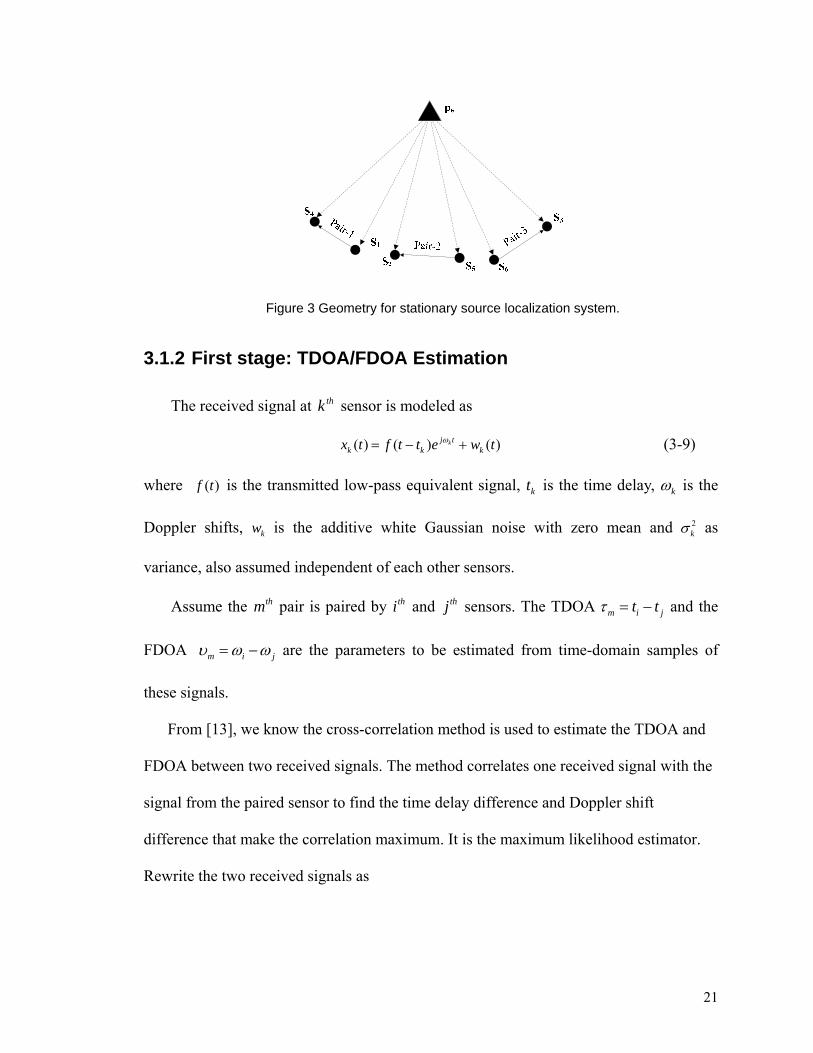
21
Figure 3 Geometry for stationary source localization system.
3.1.2 First stage: TDOA/FDOA Estimation
The received signal at thk sensor is modeled as
( ) ( ) ( )kj tk k kx t f t t e w tω= − + (3-9)
where ( )f t is the transmitted low-pass equivalent signal, kt is the time delay, kω is the
Doppler shifts, kw is the additive white Gaussian noise with zero mean and 2kσ as
variance, also assumed independent of each other sensors.
Assume the thm pair is paired by thi and thj sensors. The TDOA m i jt tτ = − and the
FDOA m i jυ ω ω= − are the parameters to be estimated from time-domain samples of
these signals.
From [13], we know the cross-correlation method is used to estimate the TDOA and
FDOA between two received signals. The method correlates one received signal with the
signal from the paired sensor to find the time delay difference and Doppler shift
difference that make the correlation maximum. It is the maximum likelihood estimator.
Rewrite the two received signals as
22
( ) ( ) ( )
( ) ( ) ( )m
i i i
j tj i m j
x t f t w t
x t f t e w tυτ
= +
= − + (3-10)
where ( ) ( ) ij ti if t f t t e ω= − . Then, use the cross-correlation method on (3-10) to estimate
the mτ and mυ which maximize the complex ambiguity function as
0
( , ) ( ) ( )T j t
i jA x t x t e dtυτ υ τ −= +∫ (3-11)
Let [ , ]Tm m mτ υ=θ be the parameter vector to be estimated, ˆmτ and ˆmυ be the estimates,
mτΔ and mωΔ be the estimation errors, then
ˆˆm m m
m m m
τ τ τ
υ υ υ
= + Δ
= + Δ (3-12)
The asymptotic properties of ML estimator gives that the PDF of mθ is Gaussian with
covariance matrix that is the CRLB of mθ , so
1~ ( , )a
mm
m
Nτυ
−Δ⎡ ⎤⎢ ⎥Δ⎣ ⎦
0 F (3-13)
where mF is the FIM of mθ . Stein’s paper [13] gives how to compute the FI for TDOA
and FDOA, and we will discuss it in more detail later.
Assume there are M pairs in the network. FIM of 1 2[ , , , ]T T T TMθ θ θ θ= will have the
block structure as
1 12 1
21 2 2
1 2
( )
M
M
M M M
⎡ ⎤⎢ ⎥⎢ ⎥=⎢ ⎥⎢ ⎥⎣ ⎦
F CI CICI F CI
F θ
CI CI F
(3-14)
where ,m nCI is the cross term FIM between thm and thn pairs, which is evaluated at
session 3.3.

23
3.1.3 Second Stage: Emitter Location Estimation
In the first stage, we estimate TDOA/FDOA of some pairs of received signals. In the
second stage, use these parameters to estimate the emitter location.
Signal Model
Let kr be the vector pointing from the emitter to the thk sensor kS , kr be the
Euclidean distance between them as
2 2( ) ( )k k k e k e k er x x y y= = − = − + −r s p (3-15)
ku be the unit vector of kr as k k kr=u r , ef be the transmitted frequency of the
transmitter, and c be the speed of light. The vectors used in TDOA/FDOA signal models
are illustrated in Figure 4.
is
is
jsjs
iu ju
ir jr
Figure 4 Vectors used in TDOA/FDOA equations illustration for one pair
The signal model of mτ and mυ are given by
( )
( )
1( )
( )
m m e i j
T Tem m e i i j j
f r rcffc
τ
υ
τ
υ
= = −
= = −
p
p u s u s (3-16)
The measurement vector m̂ in this stage is the estimation TDAO/FDOA vector of the
first stage. Assume M pairs in the network. The vector form signal model is

24
ˆ ( )e= +m f p e (3-17)
where
[ ][ ]
1 1
1 1
1 1
ˆ ˆ ˆˆ ˆ
( ) ( ) ( ) ( ) ( )
TM M
TM M
T
e e e M e M ef f f fτ υ τ υ
τ υ τ υ
τ υ τ υ
=
= Δ Δ Δ Δ
⎡ ⎤= ⎣ ⎦
m
e
f p p p p p
(3-18)
( )m ef τ p and ( )m ef υ p are defined in (3-16). Noise vector e has the Gaussian distribution
with covariance matrix 1( )−=eC F θ , where ( )F θ is defined as (3-14).
CRLB of ep
Therefore (3-17) is a deterministic signal plus Gaussian noise model, from (2-20) we
get
1
( ) ( )CRLB( ) ( )T
e ee
e e
−⎡ ⎤∂ ∂
= ⎢ ⎥∂ ∂⎣ ⎦
f p f pp F θp p
(3-19)
We call ( )e
e
∂=
∂f pH
p Jacobin matrix and evaluated as
1 1
1 1
1
( ) ( )
( ) ( )
( )
( ) ( )
( ) ( )
e e
e e
e e
e ee
eMM e M e
e e
M e M e
e e
f fx y
f fx y
f fx y
f fx y
τ τ
υ υ
τ τ
υ υ
⎡ ⎤∂ ∂⎢ ⎥∂ ∂⎢ ⎥⎢ ⎥∂ ∂⎢ ⎥
∂ ∂ ⎡ ⎤⎢ ⎥∂ ⎢ ⎥⎢ ⎥= = = ⎢ ⎥⎢ ⎥∂
⎢ ⎥⎢ ⎥∂ ∂ ⎣ ⎦⎢ ⎥∂ ∂⎢ ⎥⎢ ⎥∂ ∂⎢ ⎥
∂ ∂⎣ ⎦
p p
p pG
f pHp
Gp p
p p
(3-20)
where mG is the Jacobin matrix of the thm pair of sensors, defined by ( )m em
e
∂=
∂f pG
p and
calculated by

25
( )( )
T Ti j
T TT Tm j j j ji i i i
i jr r
⎡ ⎤−⎢ ⎥
= −−⎢ ⎥−⎢ ⎥⎣ ⎦
u uG u s u su s u s (3-21)
Rewrite the FIM of ep as
( ) ( )Tgeo e =J p H F θ H (3-22)
Estimation Method
We select Weighted Lease Square (WLS) method to estimate ep , which is to solve
{ }ˆ
ˆ ˆmin [ ( )] [ ( )]e
Te e− −
pm f p W m f p (3-23)
where 1−= eW C is the weighted matrix. It is obvious that the function vector ( )ef p is not
linear with respect to the emitter location vector ep . We need the iterative method (2-31)
or (2-32) to solve (3-23). We chose Gauss-Newton method based on: (i) Hessian matrix
nG is small enough to be negligible; (ii) Error term is small enough to make the sum
term negligible; (iii) Inclusion of the sum term can sometimes de-stabilize the iteration;
and (iv) For deducing the complexity of computation.
3.2 Importance of Signal Model
In chapter 2, we discussed that the parameter estimation procedure is to find an
optimal algorithm which satisfies some rules, such as MMSE or MVU. It is statistical
optimal, we need the statistical characteristics of the measured data. The implementation
of optimal processing for the second stage of TDOA/FDOA localization requires an
understanding of the probabilistic characteristics of the TDOA/FDOA estimates from the
first stage. From (3-22), the evaluation of FIM of ep needs the calculation of the FIM of
26
TDOA/FDOA, which is related with signal model of the emitter. In this session, we
discuss how the signal model will affect the statistical characteristics and the optimal
method. And the conclusion is one of the most important contributions of this dissertation.
Much work has been done to derive optimal TDOA/FDOA estimation methods and to
characterize the covariance matrix of the TDOA/FDOA estimates([6]~[20]).
TDOA/FDOA results were first developed in the early 1970s for the case of passively
locating underwater acoustic sources, where the accepted model for the signal is a
stationary random process, which is almost always assumed Gaussian. Then
TDOA/FDOA results were developed for the case of passively locating electromagnetic
sources, such as radar and communication transmitters. But for the electromagnetic
sources, most were deemed still as stationary random process. In fact, a deterministic
signal model may be better to apply.
3.2.1 Common and Uncommon Aspects of Acoustic and
Electromagnetic Signals
Common Aspects for Both Acoustic and Electromagnetic Signals
The model for two sampled passively-received baseband signals at two sensors is
given by
1
2
1 1 1
2 2 2
[ ] ( ) [ ]
[ ] ( ) [ ]
j nT
j nT
x n s nT e w n
x n s nT e w n
ν
ν
τ
τ
= − +
= − + (3-24)
where ( )s t is the complex envelope of the transmitted signal, 1τ and 2τ are delays and 1υ
and 2υ are Doppler shifts. The TDOA 12 1 2τ τ τ= − and the FDOA 12 1 2υ υ υ= − are the

27
parameters to be estimated from time-domain samples of these signals; we
define [ ]12 12Tτ υ=θ . For both the acoustic scenario and the electromagnetic scenario, the
accepted modeling assumptions for the noises for 1[ ]w n and 2[ ]w n are: (i) They are zero-
mean stationary random processes; (ii) They are each Gaussian; (iii) They are
independent of each other; and (iv) They are white for simplicity of our discussion. For
notational purposes we define: the signal [ ] ( ) ij nTi is n s nT e ντ= − , 1 2
TT T⎡ ⎤= ⎣ ⎦x x x and
1 2( )TT T⎡ ⎤= ⎣ ⎦s θ s s , where we explicitly show the dependence on the TDOA/FDOA
parameter vector. This much is common between the acoustic and electromagnetic
scenarios. The differences arise in what is assumed about the model for the signal [ ]is n .
Acoustic Signal Model
For the acoustic scenario the accepted modeling assumptions on [ ]is n are: (i) It is a
zero-mean stationary random processes; (ii) It is Gaussian; (iii) It is independent of each
noise process; and (iv) It need not be assumed white, although that is a common special
case that is considered. For this scenario: (i) The random process assumption is consistent
with the erratic nature; (ii) The Gaussian assumption is motivated by the central limit
theorem and makes the problem easily tractable; and (iii) The independence from the
noises is reasonable based on physical considerations.
Electromagnetic Signal Model
Signals emitted by electromagnetic sources tend to have much more regular structure
than the erratic variations seen in acoustic signals made by ocean vehicles and therefore
do not readily evoke the notion of random process. A classic example of a stationary
random process is a sinusoidal signal with uniformly distributed phase; despite the fact

28
that each realization of this process exhibits very regular structure it is a random process
and it is stationary. Similarly, radar pulse trains can be viewed as random processes for
the very same reason: they can be modeled as having random transmission parameters
(e.g., random time offset, random phase offset, etc.). However, such signals – with their
widely spaced pulses – can hardly be thought to be stationary processes (e.g., variance
within a pulse is not equal to the variance between pulses). Furthermore, they certainly
cannot be modeled as Gaussian. In such a scenario it is best to consider the signal [ ]is n to
be a deterministic signal rather than a random signal.
There is an immediate fundamental distinction between these two models. When we
consider the estimates of TDOA and FDOA, 12τ̂ and 12υ̂ , we typically wish to find
unbiased estimates that minimize ( )212 12ˆE τ τ⎡ ⎤−⎣ ⎦ and ( )2
12 12ˆE υ υ⎡ ⎤−⎣ ⎦ , where it needs to be
understood that when the signal is random these expectations are taken over the
combined ensemble of signal and noise, such as the Bayesian MSE. When the signal is
deterministic these expectations are taken over only the noise ensemble. Thus, when the
signal is random we are essentially finding the average squared error over all possible
noises and signals; when the signal is deterministic we are essentially finding the average
squared error over all possible noises for one specific signal.
3.2.2 Fisher Information for the Two Scenarios
From the above discussion we see that for both the acoustic scenario’s model and the
electromagnetic scenario’s model the received data vector x is Gaussian and has a
Gaussian PDF. The key distinction between these two scenarios that drives all the
differences in FIM, CRLB and optimum processing is the manner in which the TDOA

29
and FDOA impact the parameters of the Gaussian PDF of data vector x . For the case of
the acoustic scenario, the mean of x is zero and the covariance matrix of x has elements
drawn from the autocorrelation function; from this we see that the covariance matrix of x
depends on TDOA/FDOA, so we denote it as ( )C θ to show the dependence. In contrast,
for the case of the electromagnetic scenario, the mean of x is ( )s θ which depends on
TDOA/FDOA and the covariance matrix C of x is a block diagonal matrix of the two
individual noise covariance matrices, and therefore does not depend on TDOA/FDOA.
From this single distinction we see that the PDF for the acoustic case is
12 1 2
1 1( ; ) exp ( )(2 ) det [ ( )] 2
Tac Np
π−⎡ ⎤= −⎢ ⎥⎣ ⎦
x θ x C θ xC θ
(3-25)
and the PDF for the electromagnetic case is
[ ] [ ]12 1 2
1 1( ; ) exp ( ) ( )(2 ) det [ ] 2
Tem Np
π−⎧ ⎫= − − −⎨ ⎬
⎩ ⎭x θ x s θ C x s θ
C (3-26)
It is this difference that leads to significant differences in the structures of FIM as
well as the maximum likelihood estimators for the two cases. For the acoustic scenario
the mean of x is zero and therefore does not depend on the parameter vector; thus the
first term in (2-20) is zero and the FIM of TDOA/FDOA acJ for the acoustic scenario is
then given by
[ ] 1 11 ( ) ( )( ) ( ) ( )2ac ij
i j
trθ θ
− −⎡ ⎤∂ ∂
= ⎢ ⎥∂ ∂⎢ ⎥⎣ ⎦
C θ C θJ θ C θ C θ (3-27)
However, for the electromagnetic scenario the covariance of x does not depend on
the parameter vector; thus, the second term in (2-20) is zero and the FIM emJ for the
electromagnetic scenario is thus given by

30
[ ] ( ) ( )( )T
em iji iθ θ
⎡ ⎤ ⎡ ⎤∂ ∂= ⎢ ⎥ ⎢ ⎥∂ ∂⎣ ⎦ ⎣ ⎦
s θ s θJ θ C (3-28)
Comparing (3-27) and (3-28) we see that there is a significant difference between the
structures of the FIM for the two cases. Furthermore, as pointed out in several
publications the off-diagonal elements of the acoustic scenario FIM in (3-27) are zero
under a mild assumption of large time-bandwidth product, thus indicating that for the
acoustic scenario the optimal estimate of TDOA should be uncorrelated with the optimal
estimate of FDOA. However, the electromagnetic scenario FIM in (3-28) does not, in
general, yield this uncorrelated TDOA/FDOA condition. For example, for the case of
white noise the result in (3-28) gives the cross term Fisher Information element as[25]
* *1 1 2 22 212
1 2
1 1( ) Re ( ) ( ) ( ) ( )emn n
jnTs nT s nT jnTs nT s nTτ τ τ τσ σ
⎧ ⎫⎪ ⎪′ ′= − − − + − − −⎡ ⎤ ⎨ ⎬⎣ ⎦⎪ ⎪⎩ ⎭∑ ∑J θ (3-29)
which in general is not zero. Thus, for the acoustic case we can expect that for a pair of
sensors the optimal TDOA estimate is uncorrelated from the optimal FDOA estimate but
that should not be expected in the electromagnetic case.
An important impact of this comes when assessing the location accuracy that can be
achieved from a set of TDOA/FDOA measurements obtained from M pairs of sensors.
Assuming an ML estimator for the TDOA/FDOA values, their estimates can be taken to
be Gaussian and then the CRLB on the location estimate covariance becomes (3-22),
where ( )F θ is the FIM for all M TDOA/FDOA measurements. When performing studies
of location accuracy, we should use the correct FIM ( )F θ for TDOA/FDOA.

31
3.2.3 Maximum Likelihood Estimator for the Two Scenarios
The MLE for a vector parameter θ is defined to be the value that maximize the
likelihood function ( ; )p x θ over the allowable domain for θ . For the generalized
Gaussian case, it is given by[1]
{ } 11 1
ln ( ; ) ( )( ) ( )tr ( ) ( )[ ( )] [ ( )] [ ( )]T
gg T
i i i i
pθ θ θ θ
−− −
∂ ⎛ ⎞ ⎡ ⎤ ⎡ ⎤∂∂ ∂= − + − − − −⎜ ⎟ ⎢ ⎥ ⎢ ⎥∂ ∂ ∂ ∂⎝ ⎠ ⎣ ⎦ ⎣ ⎦
x θ C θC θ μ θC θ C θ x μ θ x μ θ x μ θ (3-30)
Notice that there are three terms in this result: one that depends on the sensitivity of
the mean to the parameters and two that depend on the sensitivity of the covariance to the
parameters. Because the acoustic and electromagnetic scenarios are two different special
cases of the generalized Gaussian scenario, we can use the result in (3-30) to find the
result for each of these two special cases.
For the acoustic scenario the mean of x is zero and therefore does not depend on the
parameter vector; thus, the partial derivatives of the log-likelihood function (LLF) are
given just two terms from (3-30) as
{ } 11ln ( ; ) ( ) ( )tr ( )ac T
i i i
pθ θ θ
−−∂ ⎛ ⎞ ⎡ ⎤∂ ∂
= − −⎜ ⎟ ⎢ ⎥∂ ∂ ∂⎝ ⎠ ⎣ ⎦
x θ C θ C θC θ x x (3-31)
This result is well known in the passive sonar literature. It is stated that for the
TDOA/FDOA case the determinant term in the first line of (3-31) does not depend on the
parameter vector; therefore, the first term in the second line of (3-31) can be ignored to
give
{ } 1ln ( ; ) ( )ac T
i i
pθ θ
−∂ ⎡ ⎤∂= − ⎢ ⎥∂ ∂⎣ ⎦
x θ C θx x (3-32)

32
For the electromagnetic scenario the covariance of x does not depend on the
parameter vector; thus, the partial derivatives of the LLF are given by the second term in
(3-30)
{ } 1ln ( ; ) ( ) [ ( )]T
em
i i
pθ θ
−∂ ⎡ ⎤∂= −⎢ ⎥∂ ∂⎣ ⎦
x θ s θ C x s θ (3-33)
Compare (3-32) and (3-33) shows that we should expect fundamental differences
between the MLE for the acoustic and electromagnetic cases. Surprisingly though, each
case results in a structure that involves pre-filtering the received signals followed by
cross-correlation. However, although both cases share this generalized correlator
structure, the pre-filtering needed for each case is quite different. For the acoustic case
the filters depend on interplay between the signal power spectra density (PSD) and the
noise PSD, whereas for the electromagnetic case the filters depend only on the noise PSD
and not on the signal structure.
The underlying assumption about the signal models (i.e., WSS Gaussian signal for the
passive acoustic case and a deterministic signal for the passive electromagnetic case)
leads to important differences in the results for the FIM, CRB, and MLE. The main
differences are that: (i) The general structures of the FIM and CRB are significantly
different; (ii) A key specific difference in the FIM/CRB structure is that unlike in the
acoustic case, for the electromagnetic case the FDOA and TDOA estimates of a signal
pair are likely to be correlated; (iii) For the electromagnetic case the MLE is an unfiltered
cross-correlator whenever the noise is white (the acoustic case requires the signal to be
white in order to remove the filters). Ignoring these differences can lead to incorrect

33
location accuracy assessments as well as improper choices when developing processing
schemes.
3.3 Characterizing TDOA/FDOA Performance for RF
Emitters
In chapter 2, we introduced the characteristics of an estimator and in the previous
session, we discussed the importance of signal model when evaluating an estimator. We
made some importance conclusions about electromagnetic signal used in the RF
TDOA/FDOA system. In this session, we use these conclusions to characterize the
TDOA/FDOA performance.
3.3.1 Evaluating the FIM of One Pair
Assume received signals
1
2
1 1 1
2 2 2
[ ] [ ] [ ]
[ ] [ ] [ ]
j nT
j nT
x n s nT e n
x n s nT e n
ν
ν
τ ω
τ ω
= − +
= − + (3-34)
where [ ]s nT is the sampled transmitted signal, and [ ], 1,2i n iω = is the AWGN received by
sensor and assume independent of each other. Vector term of (3-34) is
( , )
~ ( , )i i i i
i iNτ ν= +x s w
w 0 Σ (3-35)
Let
1 1 12
2 2 12
12 1 2 12 1 2
( ), ,
( )where ;
τυ
τ τ τ υ υ υ
⎡ ⎤ ⎡ ⎤ ⎡ ⎤= = =⎢ ⎥ ⎢ ⎥ ⎢ ⎥⎣ ⎦ ⎣ ⎦ ⎣ ⎦
= − = −
x s θx s θ
x s θ (3-36)
Then ~ ( ( ), )Nx s θ Σ , where Σ is a block diagonal matrix of the two individual noise

34
covariance matrices such as 1 2( , )diag=Σ Σ Σ .
Since we assume the RF signal is deterministic, according to (3-28)
[ ] 111
1,2 1,2
( )T
τ τ−⎛ ⎞ ⎛ ⎞∂ ∂
= ⎜ ⎟ ⎜ ⎟⎜ ⎟ ⎜ ⎟∂ ∂⎝ ⎠ ⎝ ⎠
s sF θ Σ (3-37)
Since
1 1 1 1
1,2 1 1,2 1
2 2 2 21,2
1,2 2 1,2 2
ττ τ τ τ
τττ τ τ τ
∂ ∂ ∂⎡ ⎤ ⎡ ⎤ ∂⎡ ⎤⋅⎢ ⎥ ⎢ ⎥ ⎢ ⎥∂ ∂ ∂ ∂∂ ⎢ ⎥ ⎢ ⎥ ⎢ ⎥= = =⎢ ⎥ ⎢ ⎥ ⎢ ⎥∂ ∂ ∂ ∂∂
⋅ −⎢ ⎥ ⎢ ⎥ ⎢ ⎥∂ ∂ ∂ ∂⎣ ⎦⎣ ⎦ ⎣ ⎦
s s ss
s s s (3-38)
Substitute (3-38) into (3-37), we get
[ ] 1 11 1 2 21 1 2 1 211
1 1 2 2
( ) ( ) ( )T T
F Fτ ττ τ τ τ
− −⎛ ⎞ ⎛ ⎞ ⎛ ⎞ ⎛ ⎞∂ ∂ ∂ ∂= + = +⎜ ⎟ ⎜ ⎟ ⎜ ⎟ ⎜ ⎟∂ ∂ ∂ ∂⎝ ⎠ ⎝ ⎠ ⎝ ⎠ ⎝ ⎠
s s s sF θ Σ Σ (3-39)
where ( )iF τ is the Fisher Information of the Time of Arrive (TOA) of the thi sensor,
which is evaluated as [13]
2 2
/ 2 122
2 / 2/ 2 1
2
/ 2
( ) 8
[ ]1
[ ]
rms
N
k Nrms N
k N
F N SNR B
k S kB
N S k
τ π−
=−−
=−
= × ×
=∑
∑
(3-40)
where N is the number of samples, [ ]S k is the DFT value. Following the same rule we
get
[ ] 11 1 2 212
1,2 1,2
( ) ( , ) ( , )T
F Fv
τ υ τ υτ
−⎛ ⎞ ⎛ ⎞∂ ∂= = +⎜ ⎟ ⎜ ⎟⎜ ⎟ ⎜ ⎟∂ ∂⎝ ⎠ ⎝ ⎠
s sF θ Σ (3-41)
and
[ ] 11 1 222
1,2 1,2
( ) ( ) ( )H
F Fv v
υ υ−⎛ ⎞ ⎛ ⎞∂ ∂= = +⎜ ⎟ ⎜ ⎟⎜ ⎟ ⎜ ⎟∂ ∂⎝ ⎠ ⎝ ⎠
s sF θ Σ (3-42)

35
where ( )iF υ is the Fisher Information of the Doppler of Arrive (DOA) of the thi sensor,
which is evaluated as [13]
2 2
/ 2 122
2 / 2/ 2 1
2
/ 2
( ) 8
[ ]1
[ ]
rms
N
n Nrms N
n N
F N SNR T
n s nT
N s n
υ π−
=−−
=−
= × ×
=∑
∑
(3-43)
And ( , )i iF τ υ is the cross term Fisher Information which could be evaluated as (3-29).
From the above, it is clear that FIM of θ is the summation of FIM of TOA/DOA of
each sensor of the pair as
1 1 2 2 1 2( ) ([ , ] ) ([ , ] )T Tτ υ τ υ= + = +F θ F F F F (3-44)
3.3.2 Evaluating the FIM of Two Pairs Sharing One Sensor
Three sensors make two pairs as in Figure 5. The vector form of received signal
samples is as (3-35) for 1,2,3i = .
1s1s
2s
2s
3s3s
Pair-2
Figure 5 Three sensors and two pairs
Let
1 1231 12
2 2 1 2232 12
3 3
23 2 3 23 2 3
( ), ( ) , ,
( )where ;
andττυυ
τ τ τ υ υ υ
⎡ ⎤ ⎡ ⎤⎡ ⎤⎡ ⎤ ⎡ ⎤⎢ ⎥ ⎢ ⎥= = = = = ⎢ ⎥⎢ ⎥ ⎢ ⎥⎢ ⎥ ⎢ ⎥ ⎣ ⎦ ⎣ ⎦ ⎣ ⎦⎢ ⎥ ⎢ ⎥⎣ ⎦ ⎣ ⎦
= − = −
x s θθ
x x s s θ θ θ θθ
x s θ (3-45)

36
Then ~ ( ( ), )Nx s θ Σ , where Σ is a block diagonal matrix of the three individual noise
covariance matrices such as 1 2 3( , , )diag=Σ Σ Σ Σ . FIM of θ will have the following
structure
1
2
( ) ( )( )
( ) ( )⎡ ⎤
= ⎢ ⎥⎣ ⎦
F θ CI θJ θ
CI θ F θ (3-46)
According to (3-28) the cross term FIM between pair-1 and pair-2 can be evaluated as
[ ] 111
1,2 1,3
( )T
τ τ−⎛ ⎞ ⎛ ⎞∂ ∂
= ⎜ ⎟ ⎜ ⎟⎜ ⎟ ⎜ ⎟∂ ∂⎝ ⎠ ⎝ ⎠
s sCI θ Σ (3-47)
Since
1 1
1,2 1
2 2
1,2 1,2 2
3
1,2
τ τ
τ τ τ
τ
⎡ ⎤∂ ∂⎡ ⎤⎢ ⎥ ⎢ ⎥∂ ∂⎢ ⎥ ⎢ ⎥⎢ ⎥ ⎢ ⎥∂ ∂∂ ⎢ ⎥= = ⎢ ⎥∂ ∂ ∂⎢ ⎥ ⎢ ⎥⎢ ⎥ ⎢ ⎥∂⎢ ⎥ ⎢ ⎥⎢ ⎥∂ ⎣ ⎦⎣ ⎦
s s
s ss
0s
(3-48)
and
1
2,3
2 2
2,3 2,3 2
33
32,3
τ
τ τ τ
ττ
⎡ ⎤∂ ⎡ ⎤⎢ ⎥ ⎢ ⎥∂⎢ ⎥ ⎢ ⎥⎢ ⎥ ⎢ ⎥∂ ∂∂ ⎢ ⎥= = ⎢ ⎥
∂ ∂ ∂⎢ ⎥ ⎢ ⎥⎢ ⎥ ⎢ ⎥∂∂⎢ ⎥ ⎢ ⎥
∂⎢ ⎥∂ ⎢ ⎥⎣ ⎦⎣ ⎦
s0
s ss
ss
(3-49)
Substitute (3-48) and (3-49) into (3-47), we get
[ ] 11 11 211
2 2
( ) ( )T
F ττ τ
−⎛ ⎞ ⎛ ⎞∂ ∂= =⎜ ⎟ ⎜ ⎟∂ ∂⎝ ⎠ ⎝ ⎠
s sCI θ Σ (3-50)
Following the same rule to evaluate the other items of we get ( )CI θ , it is not hard to
get

37
2( ) =CI θ F (3-51)
Therefore the cross term FIM between pairs is the same as the FIM of the shared
sensor itself. The FIM of θ is
1 2 21
2 2 32
( ) ( )( )
( ) ( )+⎡ ⎤⎡ ⎤
= = ⎢ ⎥⎢ ⎥ +⎣ ⎦ ⎣ ⎦
F F FF θ CI θJ θ
F F FCI θ F θ (3-52)
From the above discuss, the FIM of TDOA/Foes could be calculated for the
combination of the FIM of each sensors TOA/DOA itself. That is consistent with Dr.
Chen’s assessment [23].
3.4 Characterizing Location Performance for RF
Emitters
In session 3.3, we discussed about how to compute the FIM of TDOA/FDOA. And it
is obvious the estimation accuracy is only related with the received signal quality. But the
accuracy of emitter location depends on many items, not only the received signal quality
but also the geometry properties of sensors and emitter. The second aspect is the
motivation of part of this dissertation: to exploit the geometry characteristics of location
estimation and based on them to find optimal pairs.
The location estimation is subject to various types of errors. Emitter location is
estimated by some measurements, such as times of arrivals, frequencies of arrivals. The
general signal model of any measurement is
( , , )em f= p s s (3-53)
38
where s and s is the vector of participated sensors’ positions and velocities. (3-53)
defines a surface on which ep lies. The differential of (3-53) with respect to , and ep s s
gives
T T T
ee
f f fdm d d d⎛ ⎞∂ ∂ ∂⎛ ⎞ ⎛ ⎞= + +⎜ ⎟ ⎜ ⎟ ⎜ ⎟∂ ∂ ∂⎝ ⎠ ⎝ ⎠⎝ ⎠
p s sp s s
(3-54)
Errors in the measurement m , s and s will incur an error in the estimation of ep . Take
variance of both sides of (3-54) gives
2 cov( ) cov( ) cov( )T T T T
m ee e
f f f f f fσ⎛ ⎞ ⎛ ⎞∂ ∂ ∂ ∂ ∂ ∂⎛ ⎞ ⎛ ⎞ ⎛ ⎞ ⎛ ⎞= + +⎜ ⎟ ⎜ ⎟ ⎜ ⎟ ⎜ ⎟ ⎜ ⎟ ⎜ ⎟∂ ∂ ∂ ∂ ∂ ∂⎝ ⎠ ⎝ ⎠ ⎝ ⎠ ⎝ ⎠⎝ ⎠ ⎝ ⎠
p s sp p s s s s
(3-55)
This gives an overview of how all these measurements errors play in the geo-location
estimation accuracy.
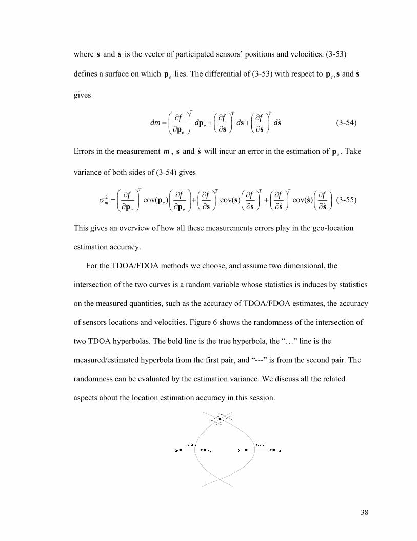
For the TDOA/FDOA methods we choose, and assume two dimensional, the
intersection of the two curves is a random variable whose statistics is induces by statistics
on the measured quantities, such as the accuracy of TDOA/FDOA estimates, the accuracy
of sensors locations and velocities. Figure 6 shows the randomness of the intersection of
two TDOA hyperbolas. The bold line is the true hyperbola, the “…” line is the
measured/estimated hyperbola from the first pair, and “---” is from the second pair. The
randomness can be evaluated by the estimation variance. We discuss all the related
aspects about the location estimation accuracy in this session.

39
Figure 6 Randomness of the intersection of two TDOA hyperbolas
3.4.1 Emitter Location Accuracy as a Function of TDOAs and
Sensor States Measurements
One TDOA value is a function of emitter location and two sensors positions as
( )1 2 1 21( , , )efc
τ = = −p s s r r (3-56)
where k e k= −r p s . One this function can define a hyperbola, and two hyperbolas define
an intersection. For the sensors as in Figure 6, the two functions are
1 1 1 2
2 2 3 4
( , , )( , , )
e
e
ff
ττ==
p s sp s s
(3-57)
Taking differentials of (3-57) and let 1 1 2
TT T⎡ ⎤= ⎣ ⎦q s s and 2 3 4
TT T⎡ ⎤= ⎣ ⎦q s s , then
1 11 1
1
2 22 2
2
T T
ee
T T
ee
f fd d d
f fd d d
τ
τ
⎛ ⎞ ⎛ ⎞∂ ∂= +⎜ ⎟ ⎜ ⎟∂ ∂⎝ ⎠⎝ ⎠
⎛ ⎞ ⎛ ⎞∂ ∂= +⎜ ⎟ ⎜ ⎟∂ ∂⎝ ⎠⎝ ⎠
p qp q
p qp q
(3-58)
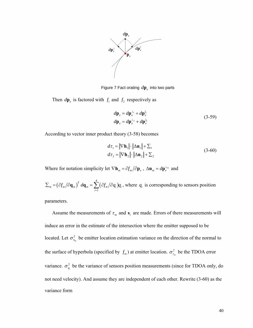
Factor edp into two parts as one is in the direction of the normal of the surface defined
by mf and noted as ed ⊥p , which is the direction as m ef∂ ∂p , the other one is
perpendicular to the normal vector and noted as edp . The fact oration is illustrated in
Figure 7.
40
edp
ed ⊥p edpep
Figure 7 Fact orating edp into two parts
Then edp is factored with 1f and 2f respectively as
1 1
2 2
e e e
e e e
d d d
d d d
⊥
⊥
= +
= +
p p p
p p p (3-59)
According to vector inner product theory (3-58) becomes
1 1 1 1
2 2 2 2
d
d
τ
τ
= ∇ ⋅ Δ +∑
= ∇ ⋅ Δ +∑
h n
h n (3-60)
Where for notation simplicity let m m ef∇ = ∂ ∂h p , mm ed ⊥Δ =n p and
( ) ( )4
1
Tm m m m m i i
i
f d f q q=
∑ = ∂ ∂ = ∂ ∂∑q q , where iq is corresponding to sensors position
parameters.
Assume the measurements of mτ and is are made. Errors of there measurements will
induce an error in the estimate of the intersection where the emitter supposed to be
located. Let 2mnσ be emitter location estimation variance on the direction of the normal to
the surface of hyperbola (specified by mf ) at emitter location. 2mτ
σ be the TDOA error
variance. 2iqσ be the variance of sensors position measurements (since for TDOA only, do
not need velocity). And assume they are independent of each other. Rewrite (3-60) as the
variance form

41
( )
( )
1 1 1
2 2 2
2 2 22
1
2 2 22
2
1
1
n
n
τ
τ
σ σ σ
σ σ σ
∑
∑
= +∇
= +∇
h
h
(3-61)
Since
Tm
m em
d∇Δ =
∇hn ph
(3-62)
Then
1ed −= Δp H n (3-63)
Where
1
1 1
22
2
,
T
T
⎡ ⎤∇⎢ ⎥∇ ⎡ Δ ⎤⎢ ⎥= Δ = ⎢ ⎥⎢ ⎥ Δ∇ ⎣ ⎦⎢ ⎥∇⎢ ⎥⎣ ⎦
hh n
H nnh
h
(3-64)
Therefore
1 1( )e
T− −Δ= np
C H C H (3-65)
where
( )
( )
1 1
2 2
2 22
1
2 22
2
1 0
10
τ
τ
σ σ
σ σ
∑
Δ
∑
⎡ ⎤+⎢ ⎥∇⎢ ⎥= ⎢ ⎥+⎢ ⎥
∇⎢ ⎥⎣ ⎦
n
hC
h
(3-66)
Computation the two important measurements of ep
C are got as
( ) ( )
( ) ( )
1 1 2 2
1 1 2 2
2 2 2 2
2
2 2 2 2
2 2 21 2
trace( )
determinant( )
e
e
τ τ
τ τ
σ σ σ σ
σ σ σ σ
∑ ∑
∑ ∑
+ + +=
+ ⋅ +=
⋅ ∇ ⋅ ∇
p
p
CH
CH h h
(3-67)

42
Put into the geometrical factors and define a new induced vector concept as
cos( 2) sin( 2)sin( 2) cos( 2)
π ππ π
⊥ ⎡ ⎤= ⋅⎢ ⎥⎣ ⎦
x x , which means ⊥x is generated by count-clockwise rotating
x by 2π degree. Define angles as following
(i) ( ) ( )1 1 2 2 3 4, and ,θ θ= ∠ = ∠r r r r
(ii) ( )( , ) ,i j i jα ⊥= ∠ r r
Then after simplification and computation (3-67) becomes
( )
( )
1 1 2 2
1 1 2 2
2 2 2 21 2
2
(1,3) (2,4) (1,4) (2,3)
2 2 2 2
2
(1,3) (2,4) (1,4) (2,3)
4(1 cos )(1 cos ) ( ) ( )trace( )
cos cos cos cos
( )( )
determinant( )cos cos cos cos
τ τ
τ τ
θ θ σ σ σ σ
α α α α
σ σ σ σ
α α α α
∑ ∑Δ
∑ ∑Δ
⎡ ⎤− − + + +⎣ ⎦=+ − −
+ +=
+ − −
n
n
C
C
(3-68)
From (3-68), the variance of estimation errors is a complex combination of both
measurement factors (all σ values) and geometrical factors (angles). Based on the
relationship of all these angles, trace( )ΔnC may be get more simplified, but even further
simpler there is not a clear optimal relationship between the trace( )ΔnC and some
specified parameters. It is also for the case of determinant( )ΔnC . And there are trade-off
among these geometrical factors.
3.4.2 Emitter Location Accuracy as a Function of FDOA and
Sensor States Measurements
One FDOA value is a function of emitter location and two sensors positions and
velocities as
43
1 1 2 21 2 1 2
1 2
( , , , , )T T
ee
fgc
υ⎛ ⎞
= = −⎜ ⎟⎜ ⎟⎝ ⎠
r s r sp s s s sr r
(3-69)
One this function can define a curve, and two FDOA measurements can define an
intersection, for the sensors as in Figure 6, the two functions are
1 1 1 2 1 2
2 2 3 4 3 4
( , , , , )( , , , , )
e
e
gg
υυ
==
p s s s sp s s s s
(3-70)
Following the same discussion as TDOA case, we can also get the similar expression
as (3-65) with different H and ΔnC matrices as
( ) ( )( ) ( )
2 22 21 1 1 1 2 2 2
21 2 1 2 1 1 2 1 1 2 2
sin sin
2 cos cos cos cos cos sin sin
α α
θ α α α β α β
∇ = +
− − −
h s r s r
s s r r(3-71)
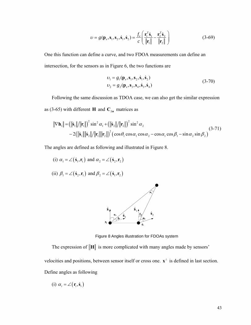
The angles are defined as following and illustrated in Figure 8.
(i) ( ) ( )1 1 1 2 2 2, and ,α α= ∠ = ∠s r s r
(ii) ( ) ( )1 2 1 2 1 2, and ,β β= ∠ = ∠s r s r
1s 1s2s
2s
Figure 8 Angles illustration for FDOAs system
The expression of H is more complicated with many angles made by sensors’
velocities and positions, between sensor itself or cross one. ⊥x is defined in last section.
Define angles as following
(i) ( ),i i iα = ∠ r s
44
(ii) ( )( , ) ,i j i jγ ⊥= ∠ r r
(iii) ( )( , ) ,i j i jλ ⊥= ∠ r s
(iv) ( )( , ) ,i j i jβ ⊥= ∠ s s
Based on these definitions, H is given as
(1,3) (1,4) (2,3) (2,4)2 2
1 2
f f f f− − +=
∇ ⋅ ∇H
h h (3-72)
where
( , ) ( , ) ( , ) ( , ) ( , )cos cos cos cos cos cos cos cosi ji j i j i j i i j j j i i j
i j
f α α γ α λ α λ β⎡ ⎤= − − +⎣ ⎦s s
r r(3-73)
Totally there are sixteen angles. Even though some of them may be represented by
some others, (3-72) is still a long expression with many items. Put (3-71) and (3-72) into
(3-67) will get two more long expressions, we do not need to give the long expression at
here.
The objective of this session is to give an explicit expression about how are all the
measurements accuracy and geometrical properties related with the emitter location
accuracy. The relationship in general form is given by (3-67). And we checked two
special case of (i) two TDOAs and (ii) two FDOAs. The purpose of these derivations is
not to give a simple relationship between the accuracy and any related parameter. It is to
give an overall insight about what will reflect our estimation accuracy. In the following
chapters we are going to discuss more about some specified errors and give out optimal
or sub-optimal solutions to solve the unexpected uncertainties.
45
3.5 Appendix 3A-Convergence of Gauss-Newton Least
Square Method
In the second stage of the data processing we use the iterative lease square method to
estimate emitter location. Given an initial reference estimation of ep , iteratively update
by (2-32). We need to consider the convergence problem.
Least Square (LS) procedure estimate model parameters θ by minimizing the LS
error criterion, or called cost function
( ) [ ( )] [ ( )]TJ = − −θ x s θ x s θ (3-74)
In general, ( )s θ is a N-dimensional nonlinear function of θ .
The Newton-Raphson iteration method is to linearize the differentiation of J , which
needs the first-order and second-order partials of ( )s θ with respect to θ . The Gauss-
Newton iteration method is to linearize ( )s θ about some nominal 0θ , which only needs
the first-order partial of ( )s θ with respect to θ . The iterative equation is
11 [ ( ) ( )] ( )[ ( )]T
k k k k k k−
+ = + −θ θ H θ H θ H θ x s θ (3-75)
where
( )[ ( )] iij
j
sθ
∂=
∂θH θ (3-76)
For small h the Taylor expansion of ( )s θ and keep up to the first order derivative
item is
( ) ( ) ( )k k k+ ≈ +s θ h s θ H θ h (3-77)

46
For notation purpose write ( )ks θ as kθ
s and ( )kH θ as kθ
H . Inserting (3-77) into
(3-74) we see that
( ) ( ) ( )
( ) ( ) 2( )k k k k
k k k k k k
Tk
T T T T
J + = − + − +
= − − + − +
θ θ θ θ
θ θ θ θ θ θ
θ h x s H h x s H h
x s x s x s H h h H H h (3-78)
Let
( ) ( )
k
kL J= += − θ
h θ hy x s
(3-79)
then
( ) 2k k k k
T T TL J= + +θ θ θ θh y H h h H H h (3-80)
The gradient and the Hessian of ( )L h with respect to h are
( ) 2 2
( ) 2k k k
k k
T T
T
L
L
′ = +
′′ =
θ θ θ
θ θ
h H y H H h
h H H (3-81)
In TDOA/FDOA emitter localization system, kθ
H can be calculated as (3-20). So
generally the columns of kθ
H are independent, therefore ( ) 2k
rank =θH , kθ
H is full rank.
So ( )L′′ h is positive definite. ( )L h has a unique minimizer and can be solved as
* 1( )k k k
T T−= − θ θ θh H H H y (3-82)
and
* *( ) ( ) ( )Tk k kJ J J ′+ ≈ +θ h θ h θ (3-83)
Since the gradient of ( )kJ θ is
( ) ( )k kkJ ′ = −θ θθ H x s (3-84)
then
47
* *
1
( ) ( )
( ) ( ) ( )
( ) ( ) 0
k k
k k k k k k
k k
T Tk
T T T
T
J−
′ = −
= − − −
= − − − <
θ θ
θ θ θ θ θ θ
θ θ
h θ h H x s
x s H H H H x s
x s x s
(3-85)
Therefore
( ) ( )k kJ J+ <θ h θ (3-86)
So h is a descent direction of J . So updating θ by 1k k+ = +θ θ h , finally the solution
can converge to the optimal one.
In this chapter, we (i) Give basic background about emitter location estimation and
discuss why we choose TDOA/FDOA methods in this dissertation; (ii) Talk about the
basic procedures of the localization; (iii) Exploit the importance of signal model and get
the important and fundamental insight about the FIM/CRLB and MLE, which is one of
this dissertation’s contribution; (iv) Based on the results we get, compute the
characteristics of TDOA/FDOA estimation; (v) Develop the geometrical factors
importance in the localization, which is the motivation of the next chapter.

48
4 Network Management---FIM Based Sensor
Selection and Pairing
Briefly, the localization procedure is: the full set of sensors is tasked to
simultaneously intercept signal data in a specified frequency band and then cooperatively
share data to detect the presence of an emitter and then to locate it. After data collection
at the sensors, they send a small amount of data to a central node where the data sets are
processed to determine which sensors detected data from the same emitter of interest.
And based upon this small amount of data, it is possible to determine a rough estimate of
the emitter location, which will be used as initial estimation at iterative lease-square
estimation.
On the basis of this initial, small amount of shared data from the remaining subset of
participating sensors, it is also possible to assess the impact of the relative emitter-sensor
geometry on the location processing task, thus allowing subsequent processing to be
optimized with respect to the geometry and error sources. Thus, the central node then
uses knowledge of the current positions and trajectories of the remaining sensors to
further reduce the participating subset based on the quality and the error sensitivity of
their data sets. For example, one sensor may have high-quality data (e.g., SNR, Fisher
information, etc.) but its position and trajectory give it a high susceptibility to non-noise
error sources (e.g., GDOP, sensor vibrations, navigation errors, etc.), another sensor
could have low-quality data but have low susceptibility to error sources, etc. By
eliminating sensors that have negligible usefulness to the final outcome of the task it is
possible to reduce the amount of network communication resources needed to accomplish

49
the task. Further reduction in the needed communication resources is then achieved
through location-optimized compression when this final subset of participating sensors
shares its data to support the location-estimation tasks[23]. Then, location processing is
completed using algorithms specifically designed to mitigate the impact of the error
sources. If at this point the accuracy of the location estimate is desired to be further
improved, it is possible to determine optimal trajectories for the selected sensor subset in
order to minimize their sensitivities to GDOP, vibration, etc. during subsequent data
collection . We briefly discussed this issue in chapter-6. We aim to provide a
comprehensive method of maximizing the effectiveness of a sub-set of networked sensors
by considering the network-wide setting in which the sensors work. The following
sections provide the details upon which these ideas are based.
4.1 Optimal Criterion
We know the Cramer-Rao Lower Bound of a parameter is depended on the signal
model. The signal model is related with both the parameters assumed known and the
ones to be estimated. Assume a signal model is a function of both α and β as ( ; )s α β ,
where α is the vector to be estimated and β is the system parameter vector which is
assumed known and can be modified. The natural and ultimate choice of criteria to
optimal an estimation algorithm relies on their error covariance matrix which is lower
bounded by the CRLB matrix, which is given in chapter 2. For example, if
1 2CRLB( ; ) CRLB( ; )<α β α β , we can say that the signal model based on 1β is better than
the one on 2β at the estimating of α point of view. For vector case, “<” means
50
2 1CRLB( ; ) CRLB( ; )−α β α β is a positive definite matrix. So if we can choose β to get
minimal CRLB of α , the optimal problem will be given as
{ }* arg min some scalar value function of CRLB ( ; )= αββ α β (4-1)
Since for the vector estimator, the CRLB is a matrix, we need some scalar value
function to evaluate the minimal of a matrix, such as eigen-values, trace or determinant.
4.1.1 Covariance Matrix and Error Ellipsoid
The covariance matrix of estimation errors can be visualized in the space of errors.
Assume θ̂ is a 1p× unbiased estimated vector and it is Gaussian with zeros mean and
covariance matrix θ̂
C . Then the PDF of θ̂ is given by
1ˆ1/ 2
ˆ
1 1ˆ ˆ ˆ( ) exp ( ) ( )2(2 )
T
pp
π−⎧ ⎫= − − −⎨ ⎬
⎩ ⎭θ
θ
θ θ θ C θ θC
(4-2)
The equal height contours of this PDF are given by the values of estimation error
vector ˆ ˆΔ = −θ θ θ such that
1ˆ
ˆ ˆT k−Δ Δ =θ
θ C θ (4-3)
From [17], choosing the value of k , such that
2 ln(1 )ek P= − − (4-4)
where eP is the probability that ˆΔθ will lie inside the ellipsoid specified by (4-3). For
example, if we want to see the ellipsoid that includes 50% estimates errors, then
2 ln(1 0.5)k = − − . The size and orientation of the ellipsoid can be described in terms of
eigenvalues and eigenvectors of the symmetric p p× matrix θ̂
C . Let the eigen-
decomposition of θ̂
C be

51
ˆ1
pT
i i iiλ
=
=∑θC v v (4-5)
where iλ is the eigenvalue, iv is the corresponding eigenvector.
For visualizing, assume 2p = and ˆ ˆ ˆ[ , ]Te ex y=θ . Therefore the vicariate covariance
matrix can be expressed as
2ˆ ˆ ˆ,
ˆ 2ˆ ˆ ˆ,
e e e
e e e
x x y
x y y
σ σ
σ σ
⎡ ⎤= ⎢ ⎥⎢ ⎥⎣ ⎦
θC (4-6)
and
( )( )
2 2 2 2 2 2ˆ ˆ ˆ ˆ ˆ ˆ1 ,
2 2 2 2 2 2ˆ ˆ ˆ ˆ ˆ ˆ2 ,
1 ( ) 421 ( ) 42
e e e e e e
e e e e e e
x y x y x y
x y x y x y
λ σ σ σ σ σ
λ σ σ σ σ σ
= + + − +
= + − − + (4-7)
The error ellipse of [ ]ˆ ˆ Te ex yΔ Δ is as in Figure 9. The lengths of the principle axes
are proportional to the value of the eigenvalues. And the directions of the principle axes
are along with the eigenvectors. It is clear, the smaller iλ , the more accurate of the
estimates, on the contrary, the larger iλ , the wider estimation error range will be.
ˆexΔ
ˆeyΔ
2kλ 1kλ
1v
2v
Figure 9 Error ellipse and coordinate axes in the
52
relationship with eigenvalues and eigenvectors.
4.1.2 Criterion Selection
There are two normally used measurements to measure the size of an ellipse, one is
the area and the other one is the perimeter. The calculations of the ellipse in Figure 9 are
given by
1 2
1 2
Area
Perimater 2
k
k
π λ λ
π λ λ
=
≈ + (4-8)
From matrix theory, the determinant of a matrix is equal to the product of the
eigenvalues, and the trace of a matrix is equal to the summation of the eigenvalues. So
the two measurements of the ellipse specified by θ̂
C are proportional to the two
important properties of θ̂
C as
ˆ
ˆ
Area Determinant( )
Perimeter Trace( )
∝
∝θ
θ
C
C (4-9)
The inverse of Fisher Information Matrix is the CRLB matrix, which is the “smallest”
matrix (as indicated in (2-17) ) that an unbiased estimator can get. From chapter 3, the
FIM of emitter location is ( ) ( )Tgeo e =J p H F θ H , which can be expended as
1 1 1
( ) ( ) ( )M M M
T Tgeo e m m m m n mn m n
m m n m= = = +
= + + +∑ ∑ ∑J p G F G G G CI G G (4-10)
The matrices are defined in (3-14) and (3-20). The first summation in (4-10) is the
combination of each pair independently and the second one is due to the cross term FIM,
if there is some sensors participated in more than one pair.
We need to optimize CRLB, which is the inverse of FIM. The expression of inverse
of (4-10) is complicated even if there is only the first summation. So instead of discussing

53
the optimal eigenvalues of CRLB, we will discuss the eigenvalues of geoJ to avoid the
complexity of calculating 1geo−J . Define the eigen-decomposition of geoJ as
1
1pT
geo i ii iλ=
=∑J v v (4-11)
To increase the accuracy of the estimates is equal to reduce the size of the error
ellipse. But which measurement we should use to be our criterion? Since the CRLB is the
inverse of FIM, based on matrix theory; the eigenvalues of them are reciprocal of each
other. Then
1
1
pT
geo geo i i ii
λ−
=
= =∑CRLB J v v (4-12)
Since geoJ is positive definite matrix, all its eigen-values 1 iλ are positive. It is easy
to show that minimizing 1
1
det( )p
geo ii
λ−
=
=∏J is equivalent to maximizing
1
det( ) 1p
geo ii
λ=
=∏J . So the decrease of the area of CRLB ellipse is equal to the increase
of the FIM ellipse.
Is that also true for the perimeter? Let 1
trace( ) 1/p
geo ii
λ=
=∑J and 1
1
trace( )p
geo ii
λ−
=
=∑J .
Using the Cauchy-Schwarz inequality [3] gives
1
11
1 1
1/ tr( )tr( )p p
p i i geo geoi i
p
pλ
λ λ λ λ
λ
−
= =
⎡ ⎤⎢ ⎥
⎡ ⎤= ≤ =⎢ ⎥⎣ ⎦ ⎢ ⎥⎢ ⎥⎣ ⎦
∑ ∑ J J (4-13)
This gives 1 2tr( ) / tr( )geo geop− ≥J J . Thus the maximization of tr( )geoJ tends to bring the
minimization of 1tr( )geo−J .

54
Based on matrix theory and (4-10)
,1 1 1
tr( ) tr( ) tr( )M M M
geo m m nm m n m= = = +
= +∑ ∑ ∑J J J (4-14)
where Tm m m m=J G FI G and , ( ) ( )T
m n m n mn m n= + +J G G CI G G . So if we choose trace of geoJ
as our optimal criterion, we can discuss pair-wise.
But the determinant of geoJ generally does not have the formula as (4-14), there is not
an explicit expression of the determinant of the summation of matrices. The Minkowski
Inequality [3] says for (4-10)
,1 1 1
det( ) det( ) det( )M M M
geo m m nm m n m= = = +
≥ +∑ ∑ ∑J J J (4-15)
with equality if and only if all the mJ and ,m nJ are positively linearly dependent. It is
complicated if we can not separate pairs.
From the above discuss, there is a trade off between choosing the determinant or the
trace of geoJ to be our optimal criterion. (i) For determinant, maximize the determinant
of geoJ definitely minimize the determinant of 1geo−J , but the expression of det( )geoJ with
respect to the parameters which we are going to optimal is complicated and hard to
discuss; (ii) For trace, based on (4-14), the trace of geoJ can be separated pair-wised,
which makes the optimal method done inside each pair, but the maximal of tr( )geoJ can
not guarantee the minimal of 1tr( )geo−J , even though it always has the tendency. We
choose trace as our criterion, since normally the structure of geoJ will satisfy the
maximization of tr( )geoJ bring the minimization of 1tr( )geo−J , and pair-wised optimization
brings more flexibility.

55
4.2 Diversity of Sensor Selection and Pairing
Each element of Fisher Information Matrix geoJ is a function of both emitter location
ep and sensor navigation data s and s , so is the trace of geoJ . Our objective is to select
an optimal subset of sensors and pair them as well. The optimal function is given by
{ } ( )( ){ }*
subsetsubset of sensors = arg max trace subsetgeoJ (4-16)
The computation of geoJ depends on how the sensors are cooperated. There are many
ways to manage a set of sensors according to the sensor network types. We propose
various approaches to this problem and discuss trade-offs between them, for example (i)
assumes that the sensors have pre-paired and share their data between these pairs; sensor
selection then consists of selecting pairs to optimize performance while meeting
constraints on number of pairs selected; (ii) consists of optimally determining pairings as
well as selections of pairs but with the constraint that no sensors are shared between pairs;
(iii) consists of allowing sensors to be shared between pairs; and etc.
4.2.1 Network Types
Wireless sensor network is the network that sensors are cooperatively monitor
physical or environmental conditions. So the sensors need to be grouped together under
some constraints. The TDOA/FDOA measurements need a set of sensors selected and
paired. There are many ways to cooperate the sensors and let them paired. The sensors
are connected according to some requirements, such as distance, effective signal noise
ratio, efficiency and etc. We define the three normally practical types of sensor network
as following and illustration is in Figure 10.

56
Type-I: No Sensor Sharing (a pair that does not share any of its sensors with any
other pairs is called “independent pair”.);
Type-II: De-Centralized Sensor Sharing (some sensors are participated in more than
one pair, and there is no center sensor.);
Type-III: Centralized Sensor Sharing (a common reference/fusion/center sensor is
used, all the other sensors are paired with it.)
Figure 10 Three type of sensor networks
Based on the different network types, the FIM of geo-location will have different
structure which is discussed later.
4.2.2 Two Pairing Scenarios
Besides the specified sensor network types we need to consider, there are also two
different scenarios for the given sensors: (i) pre-paired sensors, in which all the sensors
are already paired, we can not change their pairing topology; (ii) free sensors, a sensor
that could be paired to any other sensors is called “free sensor”, we can pair them with
more flexibility. In the following sessions, we discussed the sensor selections algorithms
for the three network types and two scenarios.

57
4.3 Sensor Selection and Pairing Strategies
In the previous session, we have discussed about the diversity of pairing strategies, in
this session we give solutions for them.
4.3.1 Pre-Paired Sensors
When sensors are pre-paired, since we could not depart the pairs and re-pair them, we
select pairs instead of sensors. We do not have much flexibility to pair the sensors. The
TDOA/FDOA pair-FIM mF and cross-FIM ,m nCI are evaluated based on the paring and
sensor sharing topology.
(1) Type-I: No Sensor Sharing
When no sensor is shared all the cross-FIM ,m nCI is zero. The mF is evaluated
individually for each pair. Then θF of all TDOA/FDOA estimation will have the block
diagonal structure as
1
2
M
⎡ ⎤⎢ ⎥⎢ ⎥=⎢ ⎥⎢ ⎥⎣ ⎦
θ
F 0 00 F 0
F
0 0 F
(4-17)
FIM of geo-location (4-10) becomes
1
( )M
Tgeo e m m m
m=
=∑J p G F G (4-18)
The problem of selecting K pairs from M pairs is specified by
{ } ( ) ( ){ }
1
*1 1 1 1 1, ,
1
, , arg min trace
. . , {0,1}M
T TM M M M Mp p
m M m
p p p p
s t p p p K M p
⎡ ⎤= ⋅ + + ⋅⎣ ⎦+ + = < ∈
G FG G F G (4-19)
It is to select the K pre-paired sensor pairs that have the largest values of trace( )mJ .
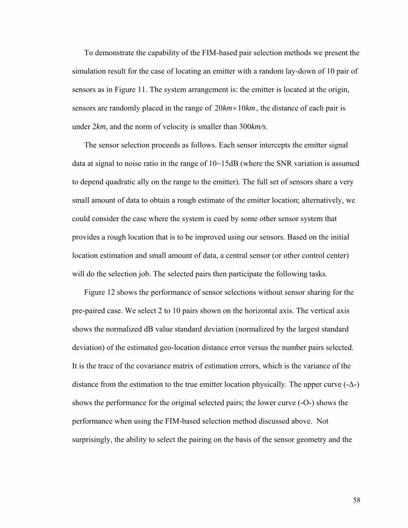
58
To demonstrate the capability of the FIM-based pair selection methods we present the
simulation result for the case of locating an emitter with a random lay-down of 10 pair of
sensors as in Figure 11. The system arrangement is: the emitter is located at the origin,
sensors are randomly placed in the range of 20 10km km× , the distance of each pair is
under 2km, and the norm of velocity is smaller than 300km/s.
The sensor selection proceeds as follows. Each sensor intercepts the emitter signal
data at signal to noise ratio in the range of 10~15dB (where the SNR variation is assumed
to depend quadratic ally on the range to the emitter). The full set of sensors share a very
small amount of data to obtain a rough estimate of the emitter location; alternatively, we
could consider the case where the system is cued by some other sensor system that
provides a rough location that is to be improved using our sensors. Based on the initial
location estimation and small amount of data, a central sensor (or other control center)
will do the selection job. The selected pairs then participate the following tasks.
Figure 12 shows the performance of sensor selections without sensor sharing for the
pre-paired case. We select 2 to 10 pairs shown on the horizontal axis. The vertical axis
shows the normalized dB value standard deviation (normalized by the largest standard
deviation) of the estimated geo-location distance error versus the number pairs selected.
It is the trace of the covariance matrix of estimation errors, which is the variance of the
distance from the estimation to the true emitter location physically. The upper curve (-Δ-)
shows the performance for the original selected pairs; the lower curve (-O-) shows the
performance when using the FIM-based selection method discussed above. Not
surprisingly, the ability to select the pairing on the basis of the sensor geometry and the

59
rough emitter location enables better performance. And for the layout as in our simulation,
only 2 pairs selection can achieve the accuracy as the 8 pairs selected originally.
-1 -0.8 -0.6 -0.4 -0.2 0 0.2 0.4 0.6 0.8 1
x 104
-10000
-8000
-6000
-4000
-2000
0
2000
1
2
3
4 5
6
7
8
9
10
1112
13
14
15
16
17
18
19
20
X Position (meter)
Y P
osi
tio
n (
met
er)
Figure 11 Layout of 10 pairs of sensor
2 3 4 5 6 7 8 9 10-30
-25
-20
-15
-10
-5
0
Number of Pairs Selected
No
rmal
ized
Sta
nd
ard
Dev
iati
on
(d
B)
Normalized Standard Deviation of Location EstimationFIM-Based Selected Pairs w/o Sharing
FIM-Based Selected PairsOriginal Selection
Figure 12 Simulation result for FIM-based sensor pairs selection w/o sharing.
The Standard deviation is normalized and taken the dB value.

60
(2) Type-II: De-Centralized Sensor Sharing
Under this type, the network looks messy. Some pairs are independent; some sensors
are participated in more than one pair. For type-I, we can treat the sensors pair by pair,
since there is no correlation when estimating TDOA/FDOAs. Here we define a group of
sensors as a sensor set by: A set is defined by a group of sensors which do not have
connections with any other sensors outside the group and do not have independent pairs
inside the group. For the sensor network in Figure 10-(b), the sets are defined as in Figure
13. Set-1 is grouped by sensor-1,2, and 4; Set-2 is grouped by sensor-3,5,6 and 7.
S4
S1 S2
S5
S3
S7
S6
Pair-1
Pair-2
Pair-4Pair-
3
Set-1
Set-2
Figure 13 Sensor sets example
We calculate the FIM of geo-location of each set. For example, the evaluation of set-1
is
, 1 1 1 1 2 2 2 1 2 1,2 1 2( ) ( )Tgeo set− = + + + +T TJ G F G G F G G G CI G G (4-20)
The problem of selecting K sensors from M sets is specified by
1
1 , 1 ,, ,
1 1 1
max { ( )}
. . , {0,1} is the number of sensors in set-i
Ngeo set M geo set Mp p
M i
i
trace p p
s t p n p n K N pn
− −⋅ + + ⋅
⋅ + + ⋅ = < ∈
J J
(4-21)
The simulation procedure and result are similar to the type-I, so we skip the result
figures.
(3) Type-III: Centralized Sensor Sharing

61
For the pre-paired case, the central sensor is already specified and the remaining N-1
sensors pair with it to form N-1 centralized pairs. The center one must be selected. How
to select the remaining K-1 sensors? They are all correlated when estimating
TDOA/FDOAs for each pair. There are 1KNC − possible ways to select K pairs. For each
selection, for illustration renumber the pair number as in Figure 14.
Figure 14 For each group, renumber each pair
The FIM of each group will have the following structure
,1 1 1
( ) ( )K K K
Tgeo k k k k m n mn m n
k m n m= = = +
= + + +∑ ∑ ∑TJ G F G G G CI G G (4-22)
Assume thr sensor is the reference one. Also the simulation procedure and result are
similar to the type-I, so we skip the result figures.
From all above, for the pre-paired sensor networks, all we can do is calculating the
FIM following some rules and select pairs. There is not much flexibility when doing the
sensor selection and pairing.
4.3.2 Free Sensors
We are given a set of sensors and asked to optimally choose a subset and the optimal
pairing them as well. In this case the pairing provides more flexibility to enable better
performance but it introduces additional complexity as well. We develop the solutions for
both no sensor sharing case and allowed sensor sharing case.
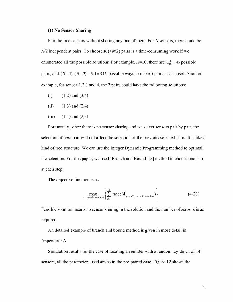
62
(1) No Sensor Sharing
Pair the free sensors without sharing any one of them. For N sensors, there could be
N/2 independent pairs. To choose K (≤N/2) pairs is a time-consuming work if we
enumerated all the possible solutions. For example, N=10, there are 210 45C = possible
pairs, and ( 1) ( 3) 3 1 945N N− ⋅ − ⋅ = possible ways to make 5 pairs as a subset. Another
example, for sensor-1,2,3 and 4, the 2 pairs could have the following solutions:
(i) (1,2) and (3,4)
(ii) (1,3) and (2,4)
(iii) (1,4) and (2,3)
Fortunately, since there is no sensor sharing and we select sensors pair by pair, the
selection of next pair will not affect the selection of the previous selected pairs. It is like a
kind of tree structure. We can use the Integer Dynamic Programming method to optimal
the selection. For this paper, we used ‘Branch and Bound’ [5] method to choose one pair
at each step.
The objective function is as
thgeo, k pair in the solutionall feasible solutions 1
max trace( )K
k=
⎧ ⎫⎨ ⎬⎩ ⎭∑ J (4-23)
Feasible solution means no sensor sharing in the solution and the number of sensors is as
required.
An detailed example of branch and bound method is given in more detail in
Appendix-4A.
Simulation results for the case of locating an emitter with a random lay-down of 14
sensors, all the parameters used are as in the pre-paired case. Figure 12 shows the

63
performance of sensor selection and pairing without sensor sharing for the free sensors
case. We select 2 to 7 pairs, shown on the horizontal axis. The vertical axis shows the
normalized dB value standard deviation of the geo-location distance error standard
derivation versus the number pairs selected. The upper curve (-Δ-) shows the
performance for the selected pairs under natural order as (1,2), (3,4) and (5,6)……; the
lower curve (-O-) shows the performance when using the FIM-based pairing method
discussed above.
2 2.5 3 3.5 4 4.5 5 5.5 6 6.5 7-20
-18
-16
-14
-12
-10
-8
-6
-4
-2
0
Number of Pairs Selected
No
rmal
ized
Sta
nd
ard
Dev
iati
on
(d
B)
Normalized Standard Deviation of Location EstimationFIM-Based Sensor Pairing w/o Sharing
FIM-Based Selected PairsOriginal Selection
Figure 15 Simulation result for 14 free sensors selection and pairing.
The standard deviation is normalized and taken the dB value.
(2) Allowed Sensor Sharing
In the sensor sharing case, some sensors will work in more than one pairs to make
more pairs and more TDOA/FDOA measurements. For N sensors, there could be 2NC
possible pairs. To choose K 2( )NC≤ pairs, there could be 2N
KC
C possible ways. For example,
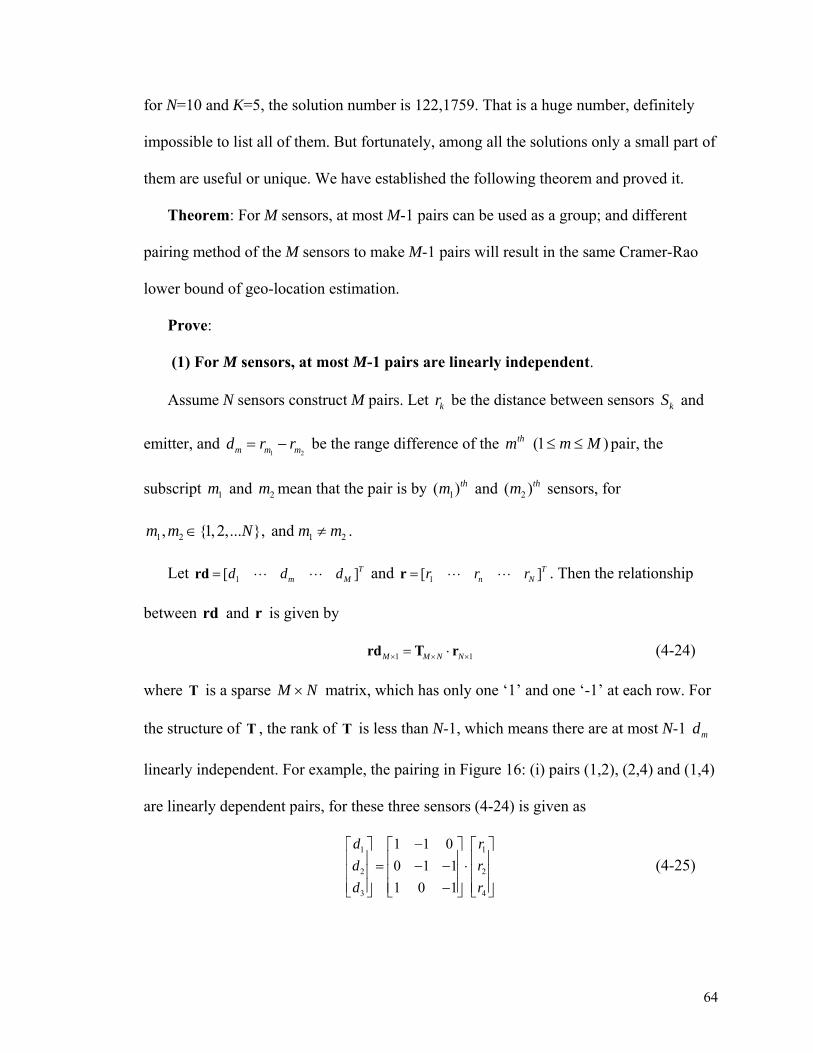
64
for N=10 and K=5, the solution number is 122,1759. That is a huge number, definitely
impossible to list all of them. But fortunately, among all the solutions only a small part of
them are useful or unique. We have established the following theorem and proved it.
Theorem: For M sensors, at most M-1 pairs can be used as a group; and different
pairing method of the M sensors to make M-1 pairs will result in the same Cramer-Rao
lower bound of geo-location estimation.
Prove:
(1) For M sensors, at most M-1 pairs are linearly independent.
Assume N sensors construct M pairs. Let kr be the distance between sensors kS and
emitter, and 1 2m m md r r= − be the range difference of the thm (1 )m M≤ ≤ pair, the
subscript 1m and 2m mean that the pair is by 1( )thm and 2( )thm sensors, for
1 2 1 2, {1,2,... }, and m m N m m∈ ≠ .
Let 1[ ]Tm Md d d=rd and 1[ ]T
n Nr r r=r . Then the relationship
between rd and r is given by
1 1M M N N× × ×= ⋅rd T r (4-24)
where T is a sparse M N× matrix, which has only one ‘1’ and one ‘-1’ at each row. For
the structure of T , the rank of T is less than N-1, which means there are at most N-1 md
linearly independent. For example, the pairing in Figure 16: (i) pairs (1,2), (2,4) and (1,4)
are linearly dependent pairs, for these three sensors (4-24) is given as
1 1
2 2
3 4
1 1 00 1 11 0 1
d rd rd r
−⎡ ⎤ ⎡ ⎤ ⎡ ⎤⎢ ⎥ ⎢ ⎥ ⎢ ⎥= − − ⋅⎢ ⎥ ⎢ ⎥ ⎢ ⎥⎢ ⎥ ⎢ ⎥ ⎢ ⎥−⎣ ⎦ ⎣ ⎦ ⎣ ⎦
(4-25)
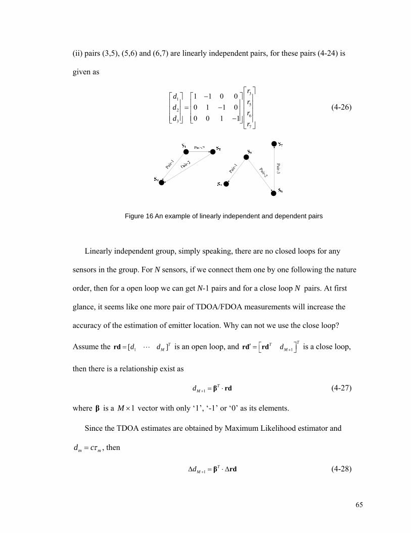
65
(ii) pairs (3,5), (5,6) and (6,7) are linearly independent pairs, for these pairs (4-24) is
given as
31
52
63
7
1 1 0 00 1 1 00 0 1 1
rd
rd
rd
r
⎡ ⎤−⎡ ⎤ ⎡ ⎤ ⎢ ⎥
⎢ ⎥ ⎢ ⎥ ⎢ ⎥= −⎢ ⎥ ⎢ ⎥ ⎢ ⎥⎢ ⎥ ⎢ ⎥− ⎢ ⎥⎣ ⎦ ⎣ ⎦
⎣ ⎦
(4-26)
Pair-
1
Pair-
1 Pair-2
Pair-3
Figure 16 An example of linearly independent and dependent pairs
Linearly independent group, simply speaking, there are no closed loops for any
sensors in the group. For N sensors, if we connect them one by one following the nature
order, then for a open loop we can get N-1 pairs and for a close loop N pairs. At first
glance, it seems like one more pair of TDOA/FDOA measurements will increase the
accuracy of the estimation of emitter location. Why can not we use the close loop?
Assume the 1[ ]TMd d=rd is an open loop, and 1
TTMd +′ ⎡ ⎤= ⎣ ⎦rd rd is a close loop,
then there is a relationship exist as
1T
Md + = ⋅β rd (4-27)
where β is a 1M × vector with only ‘1’, ‘-1’ or ‘0’ as its elements.
Since the TDOA estimates are obtained by Maximum Likelihood estimator and
m md cτ= , then
1T
Md +Δ = ⋅Δβ rd (4-28)

66
where 1Md +Δ and Δd are the estimation errors. The signal models used in the second stage
estimation will be like
1 1
( )
( )e
TM M ed f+ +
= + Δ
= + ⋅Δ
d f p d
p β d (4-29)
Therefore the error vector ' [ ]T T T= Δ ⋅Δe d β d is not i.i.d (independent identical
distribution), we can not use the Least Square method to estimate ep . Therefore the one
more pair is not able to be used. Or on the other hand, the usage of the one more
TDOA/FDOA measurements will not give any more benefit at the second stage
estimation, all its information is embedded in other pairs.
(2) Unique CRLB for a group
For M sensors, we can make as many as M-1 pairs without a close loop. For network
type-III in Figure 10, there is M-1 ways to make these M-1 pairs. We are going to prove
that the CRLB is independent of the choice of reference sensor.
Let there be a different reference sensor (RS) in each different linearly independent
group as in Figure 17. But the sensors inside each group are the same. In group-I, 3S is
the RS; in group-J, 2S is the RS.
Figure 17 An example of different choice of reference sensor
Let c be the signal propagation speed, the range difference equations is

67
kj kj k jr c r rτ= = − (4-30)
When the receivers are moving, taking time derivative of (4-30) yields a set of FDOA
measurement equation
kj kj k jr c r rτ= = − (4-31)
where ir is the rate of change of ir . From the time derivative of (3-15), ir is related to the
unknown location ep by
( )Ti e i
ii
rr
−=
s p s (4-32)
Let 1 2 1 2[ , , , , , , , ]TN Nr r r r r r=r , 1 1[ , , , , ; , , , , ] ,T
i i ki Ni i ki Nir r r r r r k i= ≠p and
1 1[ , , , , , , , , , ] ,Tj j kj Nj j kj Njr r r r r r k j= ≠p then
ii i
i
⎡ ⎤= ⋅ = ⋅⎢ ⎥⎣ ⎦
Τ 0p r H r
0 Τ (4-33)
and
jj j
j
⎡ ⎤= ⋅ = ⋅⎢ ⎥⎣ ⎦
Τ 0p r H r
0 Τ (4-34)
where iT is a ( 1)N N− × matrix, and has the following structure
[ ] ,
1, 1, 1,2,..., 1,
1, 1, 2,..., 1, 10, others
i m n
n im i n m
m i n m
− =⎧⎪ = − =⎪= ⎨ = − = +⎪⎪⎩
T (4-35)
0 is a ( 1)N N− × matrixes with all 0 entries. Let a 2( 1) 2( 1)N N− × − full rank matrix
ijQ has the structure as
ijij
ij
⎡ ⎤= ⎢ ⎥⎣ ⎦
E 0Q
0 E (4-36)
68
where ijE is the elementary matrix, which is generated by exchanging the thi and thj
rows of the identity matrix. So ijQ will satisfy
j ij i= ⋅H Q H (4-37)
then
( )j j ij i ij i i= ⋅ = ⋅ ⋅ = ⋅ =p H r Q H r Q p g p (4-38)
Based on the vector parameter CRLB transformation property [1], CRLB( )jp and
CRLB( )ip has the following relationship
( ) ( )CRLB( ) CRLB( ) CRLB( )T
Ti ij i ij i ij
i i
⎡ ⎤ ⎡ ⎤∂ ∂= =⎢ ⎥ ⎢ ⎥∂ ∂⎣ ⎦ ⎣ ⎦
g p g pp p Q p Qp p
(4-39)
Denote the emitter location ep estimated by sensor pair group-I as ˆ iep , the FIM of i
ep
is
1FIM( )i Te i i i
−= ⋅ ⋅p H C H (4-40)
where iC is the covariance matrix of TDOA/FDOA measurements calculated by
ˆ ˆE[ ]Ti i i= ⋅C p p .
Since TDOA/FDOA are estimated by ML method, we assume the covariance of the
estimates can reach CRLB, so CRLB( )i i=C p and
CRLB( ) CRLB( ) T Tj j ij i ij ij i ij= = ⋅ ⋅ = ⋅ ⋅C p Q p Q Q C Q (4-41)
jH is the Jacobin matrix of group-J defined by
( ) [ ( )] ( )j e ij i e i e
j ij ij ie e e
∂ ∂ ⋅ ∂= = = ⋅ = ⋅
∂ ∂ ∂
p p Q p p p pH Q Q Hp p p
(4-42)
Then

69
1
1
1 1 1
1
FIM( )
( ) ( ) ( )
[ ( ) ] [ ]
= FIM( )
j Te j j j
T Tij i ij i ij ij i
T T Ti ij ij i ij ij i
Ti i i
ie
−
−
− − −
−
= ⋅ ⋅
= ⋅ ⋅ ⋅ ⋅ ⋅ ⋅
= ⋅ ⋅ ⋅ ⋅
= ⋅ ⋅
p H C H
Q H Q C Q Q H
H Q Q C Q Q H
H C H
p
(4-43)
We just proved that for a group of sensors, the FIM is identical (and so is the CRLB)
if we choose network type-III to pair them, which selects one sensor as reference one. For
the sensor network type-II, there is no reference sensor. We pair all of them and avoid
any close loop. Then the matrix iT , defined as in (4-33), is a ( 1)N N− × matrix, which
only has one ‘1’ and one ‘-1’ in each row, and so does jT , which is the transform matrix
for another pairing method. The full rank matrix transform ijQ does not have a obvious
structure as in (4-35), but it is not hard to find the transform matrix and satisfies (4-37).
The following proven is the same as we prove the type-III.
We get the final conclusion, for M sensors, we can have at most M-1 pairs usable, and
the FIM/CRLB does not depend on the pairing method if there is not any close loop.
Based on this statement, it is possible to make the sensor selection and pairing. When
we are given N sensors and asked to make K pairs, there are many solutions for this
network. We can use at least 1K + sensors to make it or at most 2K sensors to make all
independent pairs. Since the main advantage to share sensors is to save some sensors
energies, we should use the number of sensors as less as possible. So here we only choose
1K + sensors to make K pairs.
For example, for given 7N = and 3K = pairs needed, compute the CRLB of geo-
location of all 47 35C = solutions, and find the one with the smallest trace. Inside each

70
solution, sensors are paired by sequence or paired by one reference sensor. For example,
as in Figure 18, the solution set is 1 2 3 4{ , , , }S S S S , the pairs are 1 2 2 3 3 4( , ),( , ), ( , )S S S S S S .
Figure 18 Example of sequence pairing and reference pairing
A simulation result for the case of locating an emitter with a random lay-down of 10
sensors (all the parameters used are as in the pre-paired case) is given in Figure 19. It
shows the performance of sensor selection and pairing with sensor sharing for the free
sensors case. For the given 10 sensors, we make 2 to 9 pairs, shown on the horizontal axis.
The vertical axis shows the normalized dB value standard deviation of the geo-location
distance error standard derivation versus the number pairs selected. The upper curve (-Δ-)
shows the performance for some randomly selected pairs; the lower curve (-O-) shows
the performance when using the FIM-based pairing method discussed above.

71
2 3 4 5 6 7 8 9-9
-8
-7
-6
-5
-4
-3
-2
-1
0
Number of Pairs Selected
No
rmal
ized
Sta
nd
ard
Dev
iati
on
(d
B)
Normalized Standard Deviation of Location EstimationFIM-Based Sensor Pairing w/ Sharing
FIM-Based Selected PairsOriginal Selection
Figure 19 Simulation result 10 free sensors selection and pairing with sensor sharing.
The standard deviation is normalized and taken the dB value.
4.3.3 Trade Off Between Non-Sharing and Sharing Methods
(1) Without Sensor Sharing
• FIM of Geo-Location is easy to calculate, since each pair is independent;
• However, the pairing method is more complicated, since we need to consider
all the possible paring ways;
• From a system point of view, the communication among different pairs can be
done simultaneously;
• The number of pairs needed is small; beyond a certain point the accuracy
improves slowly as more pairs are selected to participate.
(2) With Sensor Sharing

72
• For a total of N sensors we can have as many as 1N − pairs, the more the
higher accuracy of location estimation;
• Fortunately, FIM of all the possible independent sets are the same, so we do
not need to consider about the pairing method. One simple way is to pair the
sensors in nature order. This is the main result of this work and leads to a
major reduction in the optimization processing required.
• However, since not all the pairs are uncoupled, there are cross terms in the
TDOA/FDOA FIM. This complicates the computation required to support the
optimization processing.
• Some sensors work in more than one pair, the communication among them
needs to be considered carefully to avoid collision. This will be the focus of
future work.
Appendix-4A an Example of Branch and Bound Method
Used in Sensor Pairing
Branch and Bound method [5] is based on that the enumeration of integer solutions
has a tree structure. At each step, a decision will be made on one integer variable. The
main idea in branch and bound is to avoid growing the whole tree as much as possible.
When a node is selected for further growing, it is like branching. Not all nodes are going
to be evaluated, some are pruned in the intermediate steps.

73
Instead of enumerating all possible solutions, in each step to choose the next pair, we
grow the only ‘better’ ones. By ‘better’, we mean whose have the higher probability to be
optimal.
For 8N = , there are 28 possible pairs, randomly give each possible pair a value. (n, m)
means the pair is paired be sensor-n and sensor-m. In the first step to choose the first pair,
without loss of generality, we choose the pairs which have sensor-1 as one part. For
example, if we choose pair (1,2) as the first pair, then the bounding function value for it is
71, which let pair (3,5)-(3,6)-(7,8) as the following choosing pairs. Since sensor-1 and
sensor-2 are actually paired, we did not let them to reuse in the bounding function
calculation at this node or any descendent nodes. The very best objective function value
that we might have at a leaf node descended from (1,2)-?-?-? is 71. Sine sensor-3 is
shared between two pairs, this solution is not feasible, but maybe needed to be fathomed,
it depends on the incumbent we maybe find later. Based on this decision strategy, we got
the bud nodes in the first step of the tree as Figure 20
Figure 20 First step tree structure
The first step of the tree is generated from the root node by enumerating all the
possible pairs which have sensor-1. By evaluate the bounding function, we get our first

74
best infeasible solution, (1,5)-(2,4)-(3,6)-(7,8) , as incumbent=70. And prune the pair(1,6)
and (1,8), whose bounding function value are smaller than incumbent.
Pruned nodes are indicated by dashed border, incumbent node is by bold border, and
infeasible nodes, whose bounding function value are larger than incumbent, are going to
be growing in some order.
Since we are using the global-best node selection policy and the objective function is
to maximize, we choose pair (1,7) , who has the largest bounding function value, for first
further expansion, which gives the next tree step as Figure 21
Figure 21 Second step tree structure
The expansion of pair(1,7) is at the second step of the tree. It is generated from the
(1,7) node by enumerating all the possible pairs which have sensor-2, this is based on
nature order. After evaluating all the bounding function values, some nodes were pruned.
But we did not find a new incumbent in this expansion. Also the global-best node
selection policy, after comparing all the bounding function values of current remaining
nodes, partial solution (1,7)-(2,4) is to be fathomed next, which gives the result as Figure
22.
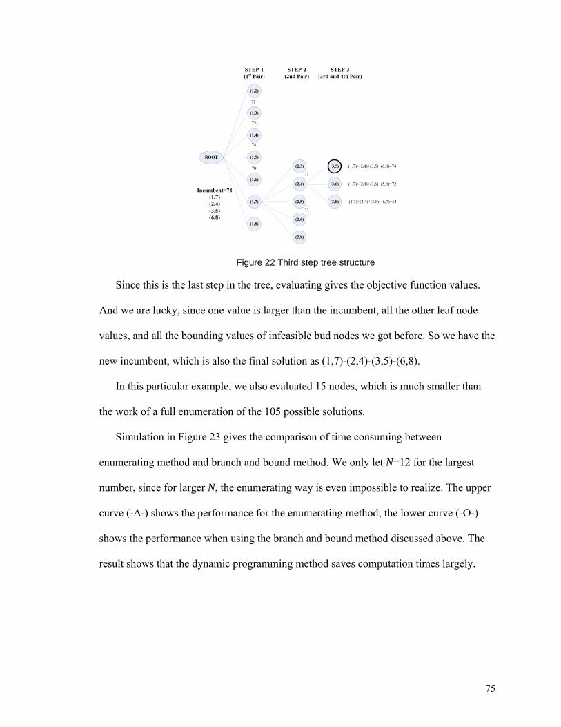
75
(1,2)
(1,8)
(1,7)
(1,6)
(1,5)
(1,4)
(1,3)
71
Incumbent=74(1,7)(2,4)(3,5)(6,8)
STEP-1(1st Pair)
ROOT
73
74
70 (2,3)
(2,4)
(2,5)
(2,6)
(2,8)
STEP-2(2nd Pair)
73
(3,5)
(3,6)
(3,8)
(1,7)+(2,4)+(3,5)+(6,8)=74
(1,7)+(2,4)+(3,6)+(5,8)=72
(1,7)+(2,4)+(3,8)+(6,7)=64
71
STEP-3(3rd and 4th Pair)
Figure 22 Third step tree structure
Since this is the last step in the tree, evaluating gives the objective function values.
And we are lucky, since one value is larger than the incumbent, all the other leaf node
values, and all the bounding values of infeasible bud nodes we got before. So we have the
new incumbent, which is also the final solution as (1,7)-(2,4)-(3,5)-(6,8).
In this particular example, we also evaluated 15 nodes, which is much smaller than
the work of a full enumeration of the 105 possible solutions.
Simulation in Figure 23 gives the comparison of time consuming between
enumerating method and branch and bound method. We only let N=12 for the largest
number, since for larger N, the enumerating way is even impossible to realize. The upper
curve (-Δ-) shows the performance for the enumerating method; the lower curve (-O-)
shows the performance when using the branch and bound method discussed above. The
result shows that the dynamic programming method saves computation times largely.
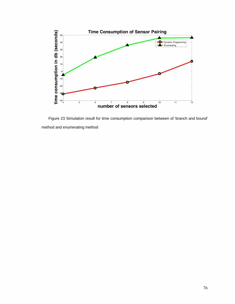
76
4 5 6 7 8 9 10 11 12-40
-30
-20
-10
0
10
20
30
40
50Time Consumption of Sensor Pairing
number of sensors selected
tim
e co
nsu
mp
tio
n in
db
(se
con
ds)
Dynamic Programming
Enumerating
Figure 23 Simulation result for time consumption comparison between of 'branch and bound’
method and enumerating method

77
5 Sensors’ Navigation Data Error Effects and
Mitigation
The signal model used in the second stage estimation depends on the sensors
positions and velocity. And we have discussed in session 3.4 that the accuracy of emitter
location is sensitive to the accuracy of sensors navigation data (NAV). Besides the
TDOA/FDOA estimation errors, sensors’ NAV errors can also lead to the emitter
location errors. In practice, the sensor navigation data can not be known exactly, there is
always error. This issue has been considered for a while, for example in [39], they
analyzed the NAV errors effects and gave a closed form solution to solve this problem.
But the algorithms are not simple and have many assumptions and simplifications. In this
section, we will develop how the errors affect the estimation accuracy and the updated
CRLB of geo-location. And we will take the navigation data errors into account when
doing the second stage estimation to reach the updated CRLB.
5.1 Least-Squares Estimation Error Model
At the second stage estimation, we used non-linear least square method to estimate
the geo-location. The signal model errors along with the measurement errors will impact
in this stage.
Assume the thm pair is paired by the (m,1)th and (m,2) th sensors, the signal model for
TDOA mτ and FDOA mω are given by
78
,1 ,2
,1 ,1 ,2 ,2
1 (|| || || ||)
( )
m e m e m
T Tem m m m m
cfc
τ
υ
= − − −
= ⋅ − ⋅
p s p s
u s u s (5-1)
Define the sensors’ parameter vector for the thm pair as ,1 ,1 ,2 ,2[ , , , ]T T T T Tm m m m m=β s s s s . Then
(5-1) can be written as
( , )
( , )m m e m
m m e m
f
f
τ
υ
τ
υ
=
=
p β
p β (5-2)
The TDOA/FDOA measurements are modeled as being corrupted by an additive
noise vector [ , ]Tm m mτ υ= Δ Δe . It also is not possible to know the sensors’ position and
velocity (the navigation data) without errors; thus they are modeled as being corrupted by
an additive error vector ,1 ,1 ,2 ,2[ , , , ]T T T T Tm m m m m= Δ Δ Δ Δη s s s s . Vector forms of the quantities of
interest at the total M pairs measurements are denoted as
1 1
1 1 1
1 1
( , )( , )
, ( , )( , )( , )
,
e
e
e
M M e M
M e M
M M
ff
ff
τ
υ
τ
υ
⎡ ⎤⎢ ⎥⎡ ⎤ ⎢ ⎥⎢ ⎥ ⎢ ⎥= =⎢ ⎥ ⎢ ⎥⎢ ⎥⎣ ⎦ ⎢ ⎥⎢ ⎥⎣ ⎦
⎡ ⎤ ⎡ ⎤⎢ ⎥ ⎢ ⎥= =⎢ ⎥ ⎢ ⎥⎢ ⎥ ⎢ ⎥⎣ ⎦ ⎣ ⎦
p ββ p β
Β f p Ββ p β
p β
e ηe N
e η
(5-3)
And then the TDOA/FDOA vector [ ]1 1T
M Mτ υ τ υ=m , measurement vector is
m̂ , and the sensors’ navigation data estimation vector become, respectively as
ˆ ( , )e= +m f p Β e (5-4)
and
ˆ = −Β Β N (5-5)

79
The emitter location problem then becomes: given TDOA/FDOA measurement
vector m̂ and the local state estimate vector Β̂ , and also a reference location 0ep (Which
could be an estimate of ep determined from a previous iteration of the estimation
procedure or based upon a priori information.) compute an estimate ˆ ep of ep . The goal
of this section is to characterize the impact of using Β̂ in this processing rather than the
unavailable actual Β .
Since ( , )ef p Β is a nonlinear vector function with respect to ep . To get a reasonably
simple estimator, ( , )ef p Β can be linearized by expanding it in a Taylor expansion about
0ep and retaining the first two terms as
0 0( , ) ( , ) ( )e e e e≅ + −f p Β f p Β H p p (5-6)
where 0
( , )
e e
e
e =
∂=
∂p p
f p ΒHp
. Combining (5-6) and (5-4) gives
e= ⋅ +r H p e (5-7)
where 0 0ˆ ( , )e e= − + ⋅r m f p Β H p .
The least square approach is to solve
[ ] [ ]{ }ˆ arg mine
Te e e= − ⋅ − ⋅
pp r H p W r H p (5-8)
Thus the solution of (5-8) is
( )
( )
1
10 0
ˆ
ˆ ( , )
T Te
T Te e
−
−
= ⋅
⎡ ⎤= + −⎣ ⎦
p H WH H W r
p H WH H W m f p Β (5-9)
Substituting (5-4) into (5-9) and rearranging terms, the expression of ˆ ep can be
written in the form
( ) ( )1ˆ T T
e e H
−= + Δ +p p H WH H W f e (5-10)
80
where 0 0( , ) ( , ) ( )H e e e eΔ = − − −f f p Β f p Β H p p is the signal model linearization error.
We assume the exact knowledge of system parameter vector Β at the above analysis
up to (5-10). If Β̂ is sufficiently close to Β , then the Taylor expansion with respect to Β
yields
ˆ ˆ( , ) ( , ) ( )e e≅ + −f p Β f p Β K Β Β (5-11)
where ˆ
( , )e
=
∂=
∂ Β Β
f p ΒKΒ
. Substitute (5-11) into (5-9) and rearranging terms, the
expression of ˆ ep can be written in the form
( ) ( )1ˆ T T
e e H K
−= + Δ + Δ +p p H WH H W f f e (5-12)
where ˆ( )KΔ = − =f K Β Β KN is the error caused by the sensors’ navigation data (system
parameters) uncertainty.
It is clear that the estimation error is composed by there error items: (i) linearization
error 1 H= Δn f ; (ii) the signal models error 2 K= Δn f ; (iii) the TDOA/FDOA measurement
error 3 =n e .
The bias of the estimator is
{ } ( ) { }1ˆE ET T
e e H K
−− = ⋅ Δ + Δ +p p H WH H W f f e (5-13)
And the covariance matrix of estimation error is given as
{ } ( ) { } ( )1 1ˆvar varT T T
e e H K
− −⎡ ⎤ ⎡ ⎤− = ⋅ Δ + Δ + ⋅⎢ ⎥ ⎢ ⎥⎣ ⎦ ⎣ ⎦p p H WH H W f f e WH H WH (5-14)
Since we use the iterative method to update the estimation, the linearization error HΔf
can be ignored at the final step. For the signal model error, there are two cases we need to
discuss about: (i) If Β is nonrandom, then the uncertainty of it will contribute to the bias
of the estimator, since { }E K KΔ = Δf f . But it will not affect the covariance matrix of
81
estimation error, since { }var KΔ =f 0 ; (ii) If Β is random and has zeros mean and
covariance matrix NC , then the estimation bias only depend on e . And assume N is
independent with e , let { }1 var− = =eW C e , then the estimation error covariance matrix
become to
{ } ( ) ( ) ( )1 1 11 1 1 1 1
1 1 1
ˆvar
T T T Te e
T
− − −− − − − −Δ
− − −
− = +
= +
e e e f e ep p H C H H C H H C C C H H C H
X X YZY X (5-15)
where
1
1
T
T
T
−
−
e
e
N
X H C H
Y H C
Z KC K
(5-16)
Compare with the case without sensor uncertainty, we can see the second term in
{ }ˆvar e e−p p is the increased variance. The trace of the second term of (5-15) is the
decrease of accuracy due to the sensor states uncertainty.
From the above discussion, in the second stage estimation, if the sensor local state
errors do not take into account, the effected item is the Jacobian matrix H . That is the
system matrix used in the iterative least square estimation for the second stage processing
contains errors due to the navigation data uncertainty. A generalized least square, called
Total Least Square (TLS) is usually used to solve this kind of problems. In appendix-4A,
we introduce this method and find out whether it will not be applied to our problem. And
we develop a new solution to solve this system uncertainty problem later.
5.2 CRLB Revisit
We know if there is no sensor navigation data uncertainty, Fisher information matrix
of emitter location is calculated as
82
1 1( , ) ( , )FIM( )e
TTe e
ee e
− −⎡ ⎤ ⎡ ⎤∂ ∂= =⎢ ⎥ ⎢ ⎥∂ ∂⎣ ⎦ ⎣ ⎦
e e
p
f p Β f p Βp C H C Hp p
(5-17)
where all the matrices are defined previously. But since we do not know Β exactly, the
uncertainty of Β will be counted into the CRLB of ep . So we need to re-evaluate the
FIM of ep based on the evaluation of FIM of TT T
e⎡ ⎤⎣ ⎦p Β . There are two signal models
related with ep and Β as
ˆ ( , )ˆ
e= +
= +
m f p Β e
Β Β N (5-18)
The measurement vector is ˆˆTT T⎡ ⎤= ⎣ ⎦α m Β . And we assume N is AWGN with zero
mean and covariance matrix NC ; N and e are independent. Then the PDF of α is given
by
( )( ) ( )[ ] [ ] ( ) ( )1 1
1 2
ˆˆln ;
ˆˆln ; ln ;
1 1 ˆ ˆˆ ˆ( , ) ( , )2 2
T TT T T T
TT Te
TTe e
p
p p
α α− −
⎡ ⎤ ⎡ ⎤⎣ ⎦⎣ ⎦
⎡ ⎤= +⎣ ⎦
= − − − + − − −e N
m Β m Β
m p Β Β Β
m f p Β C m f p Β Β Β C Β Β
(5-19)
where (if assume N sensors, M pairs and two-dimensional case)
1 21/ 2 1/ 22 4
1 1 and (2 ) (2 )M N
α απ π
= =e NC C
(5-20)
The FIM of TT T
e⎡ ⎤⎣ ⎦p Β will have the block structure as
( ) FIM( ) Cross_FIM( , )FIM ,
Cross_FIM ( , ) FIM( )T e eT T
e Te
⎡ ⎤⎡ ⎤ = ⎢ ⎥⎣ ⎦
⎣ ⎦
p p Βp Β
p Β Β (5-21)
then we can evaluate each block individually.
Apply the FIM of AWGN case on (5-19), get
83
1 1( , ) ( , )FIM( )T
Te ee
e e
− −⎡ ⎤ ⎡ ⎤∂ ∂= =⎢ ⎥ ⎢ ⎥∂ ∂⎣ ⎦ ⎣ ⎦
e ef p Β f p Βp C H C H
p p (5-22)
and
1 1 1 1( , ) ( , )FIM( )T
Te e− − − −∂ ∂⎡ ⎤ ⎡ ⎤= + = +⎢ ⎥ ⎢ ⎥∂ ∂⎣ ⎦ ⎣ ⎦e N e N
f p Β f p ΒΒ C C K C K CΒ Β
(5-23)
and
1 1( , ) ( , )Cross_FIM( , )T
Te ee
e
− −⎡ ⎤∂ ∂⎡ ⎤= =⎢ ⎥ ⎢ ⎥∂ ∂⎣ ⎦⎣ ⎦e e
f p Β f p Βp Β C H C Kp Β
(5-24)
The CRLB matrix of TT T
e⎡ ⎤⎣ ⎦p Β will also have the block structure as
( ) ( ) 1
CRLB , FIM ,
CRLB( ) Cross_Covariance( , )Cross_Covariance ( , ) CRLB( )
T TT T T Te e
e eT
e
−⎡ ⎤⎡ ⎤ ⎡ ⎤=⎣ ⎦ ⎣ ⎦⎢ ⎥⎣ ⎦
⎡ ⎤= ⎢ ⎥⎣ ⎦
p Β p Β
p p Βp Β Β
(5-25)
Substitute (5-22), (5-23) and (5-24) into (5-21), and the matrix theory gives the
CRLB of ep as
( ) 11 1 1 1CRLB( ) T Te
−− − − −= + −p X X Y Z Y X Y Y X (5-26)
where , and X Y Z have the same definition as (5-16).
The above analysis indicates that when there is sensor local state uncertainty, the
CRLB of ep will have one more term compare with the case without uncertainty. If we
do not consider this uncertainty in our second stage estimation, the estimation covariance
matrix can not reach the CRLB.

84
5.3 Updated Weighted Matrix
When we do not consider about the sensors’ navigation data uncertainty, the
weighted matrix is only related with the TDOA/FDOA measurement errors. And the
estimation variance is (5-15). Ignore the linearization error HΔf , then (5-12) becomes
( ) ( )1ˆ T T
e e
−− = +p p H WH H W e KN (5-27)
Update the weighted matrix W to
{ }1 var T− = + = +e NW e KN C KC K (5-28)
then
{ } ( )
( )
11
11 1 1 1
ˆvar
T Te e
T T
−−
−− − − −
⎡ ⎤− = +⎢ ⎥⎣ ⎦
= + −
e Np p H C KC K H
X X Y Z Y X Y Y X (5-29)
where and X Y Z are defined as (5-16).
The trace of the second term of (5-29) comparing to the trace of the second term of
(5-15) is the increased accuracy for geo-location estimation, if we use 1 T− = +e NW C KC K
instead of 1− = eW C .
And also when the navigation date error vector is AWGN and Β̂ is close enough to
Β , if we use (5-28) as the weighted matrix, the covariance matrix of ep can reach the
CRLB of ep as in (5-26).
5.4 Estimation Accuracy with Local State Error
In the previous session, we developed the updated CRLB of geo-location under the
case with sensors’ states uncertainty and give a solution to reach it. In chapter 3, we have

85
discussed all the related items of emitter location accuracy, but we do not develop more
details about to what extent sensor local states estimation errors will contribute to the
estimation accuracy. In this section, we analyze the sensitivity of the estimation accuracy
with respect to local state. From (3-60), the uncertainty caused by sensors navigation data
is as
T
mm m
m
f d⎛ ⎞∂
∑ = ⎜ ⎟∂⎝ ⎠β
β (5-30)
And for notation simplicity, we discuss one pair only and assume the pair is paired by
sensors 1S and 2S . All the typical values of sensors’ navigation data are from ?????
5.4.1 TDOA
The TDOA signal model is influenced by sensor position vector 1 2
TT Tm ⎡ ⎤= ⎣ ⎦β s s only.
T
m mm m m
m m
τ τ ⊥⎛ ⎞∂ ∂∑ = Δ = ⋅ Δ⎜ ⎟∂ ∂⎝ ⎠
β ββ β
(5-31)
where m mτ∂ ∂β is the gradient vector of mτ with respect to mβ . And m⊥Δβ is the
component of mΔβ in the direction of m mτ∂ ∂β , which is the normal to the surface
defined by mτ . Then
2
22m
mm
m
τ ⊥∑
∂∂ = ⋅ Δ
∂β
β (5-32)
The uncertainty in mβ is reflected in mτ through
1
2
1 2m
m c cτ ⎡ ⎤−∂
= =⎢ ⎥∂ ⎣ ⎦
uβ u
(5-33)

86
And the typical error of position of the on-board navigation system is mΔs is 10meter.
Then
2 2010 2m c c∑∂ ≈ ⋅ = (5-34)
5.4.2 FDOA
The FDOA signal model is influenced by both sensor position vector 1 2
TT Tm ⎡ ⎤= ⎣ ⎦β s s
and velocity vector 1 2
TT Tm ⎡ ⎤= ⎣ ⎦β s s . And can be evaluated from
22
222m
m mm m
m mm
υ υ⊥ ⊥∑
∂ ∂∂ = ⋅ Δ + ⋅ Δ
∂ ∂β β
β β (5-35)
where m mυ∂ ∂β , m mmυ∂ ∂β are the gradient vectors of mυ with respect to mβ , mmβ
respectively. The uncertainty in mβ is reflected in mυ through
1 1 1 1
1 1 2
1 22 2 2 2
2
T
m e eT
m
rf fc c r r
r
υ⎡ ⎤−⎢ ⎥ ⎛ ⎞∂ ⎢ ⎥= ≤ +⎜ ⎟⎢ ⎥∂ − ⎝ ⎠⎢ ⎥⎢ ⎥⎣ ⎦
s u s us s
β s u s u (5-36)
For the typical values of kr and || ||ks , which are 50km and 250m/s, 1 1 2 2|| || || ||r r+s s is on
the order of 210 2 / s− .
The uncertainty in mmβ is reflected in mυ through
1
2
2m e e
mm
f fc c
υ ⎡ ⎤∂= =⎢ ⎥∂ −⎣ ⎦
uβ u
(5-37)
The typical error of velocity of the on-board navigation system is kΔs is 0.02m/s.
Therefore

87
22(10 10 0.02) 2(0.1 0.02)m
e ef fc c
−∑∂ ≈ ⋅ + ≈ + (5-38)
Compare (5-34) and (5-38) reveals that the influence of uncertainty of position on
TDOA can be ignored comparing with the effects of uncertainty of position and velocity
on FDOA.
5.5 Appendix-5A Total Least Square Method for NAV
Data Errors
5A.1 Introduction of TLS
Least Squares
In order to introduce TLS, we briefly talk about some basic points about LS.
Assuming signal has linear model on the parameter vector θ as
=s Hθ (5-39)
where H is a known N p× matrix ( )N p> of full rank. The matrix H is refereed to as
the observation/system matrix. Knowing H and s we should be able to find the
parameter vector θ that made the observable s , since range( )∈s H . However, in practice
we often only have imperfect knowledge of s due to the measurement error, which is
= + Δs s s . Then we are going to solve =s Hθ . There is no solution for this equation,
since range( )∉s H . Then the problem is: Given the matrix H and the imperfect s , find
an appropriate estimate of θ . The LS approach finds an estimate θ̂ such that the residual
defined as ˆ= −r Hθ s has minimum norm; that is, 2
ˆ −Hθ s is minimized. In other words:
88
Least Square: Minimize 2
r subject to range( )+ ∈s r H and then find the θ̂ that
satisfies ˆ+ =s r Hθ .
Total Least Squares
The signal model is still as (5-39), but H is perturbed by system errors to be
= + ΔH H H . We are going to solve =s Hθ . There is no solution for this equation either,
since range( )∉s H . Recall that for standard LS we sought to find a minimum norm
vector r that would bring s back into range( )H . Here we seek simultaneously to find a
vector r and a matrix E such that
range( )+ ∈ +s r H E (5-40)
Then the total least square can be viewed as:
Total Least Square: Find the smallest perturbations r and E such that
range( )+ ∈ +s r H E and then find the θ̂ that satisfies ˆ( )+ = +s r H E θ .
The criterion taken in TLS to measure the joint size of perturbations r and E is to
form the ( 1)N p× + matrix [ ]|=Δ E r , and measure the size of Δ in some sense. The
norm of a matrix is used for this purpose. There are many matrix norms that can be
defined, but the one used here for TLS is the Fresenius norm that
2ijF
i j= Δ∑∑Δ (5-41)
Then the definition of TLS can be rewritten as:
Total Least Square: Minimize [ ]|F
E r subject to range( )+ ∈ +s r H E and then find
the θ̂ that satisfies ˆ( )+ = +s r H E θ .
The equation to solve is

89
( )+ = +s r H E θ (5-42)
which can be rewritten as
( ) ⎡ ⎤+ =⎢ ⎥−⎣ ⎦
θA Δ 0
1 (5-43)
where |⎡ ⎤= ⎣ ⎦A H s . To get a nontrivial solution to (5-43) requires that Δ be such that
+A Δ is rank deficient. That is to find = +A A Δ such that A is the closest rank-
deficient matrix to A . Then the definition of TLS can be rewritten as:
Total Least Square: Find the smallest perturbation Δ that makes |⎡ ⎤= +⎣ ⎦A H s Δ
rank deficient then find the θ̂ such that ˆ[ , ]T T T= −β θ 1 is in the null space of A .
Matrix theory says that such a matrix A% is found by replacing the smallest singular
value of A by zero. Thus, the vector that solves =Aβ 0% must be orthogonal to the
singular vectors of A that remain in A% . Since the singular vector v removed from A to
make A% is orthogonal to the singular vectors that remain in A% , it must satisfy =Av 0% .
Thus, β is proportional to v , and all that is needed is to make the last entry in v be –1 to
get the form needed for β . So if we take v and divide all of its elements by the negative
of its last element we get β .
We know the weighted LS (WLS) is used to normalize the residue. So
correspondingly there is a WTLS method. Let W be a given N N× left-side weighting
matrix and T be a given ( 1) ( 1)p p+ × + right-side weighting matrix. Then the WTLS
becomes to:
Weighted TLS: Minimize F
TrEW ]|[ subject to range( )+ ∈ +s r H E%% and then find
the θ̂ that satisfies ˆ( )+ = +s r H E θ%% .

90
Performance of Total Least-Squares
The problem to be solved is =s Hθ%% , where N p×H% and 1N×s% are perturbed versions of
some H and s . We will assume that the perturbations have uniform levels in all columns
of H% and s% ; this uniformity may have been achieved through the weighting matrices W
and T . We also assume that H% has full rank. For notational purposes, define the
following singular value decompositions:
1 1
1 1
1 1[ | ] [ | ]
p pT T
i i i i i ii i
p pT T
i i i i i ii i
σ σ
σ σ
= =
+ +
= =
′ ′ ′ ′ ′ ′= =
= =
∑ ∑
∑ ∑
H u v H u v
H s u v H s u v
% % % %
% % % % %
(5-44)
The performance advantage of TLS compared to LS has been studied and it has been
shown that, for the assumptions made above, TLS performs better than LS when
2
2
1[ | ]
p
p
σσ
⎡ ⎤ ⎡ ⎤Δ⋅ >⎢ ⎥ ⎢ ⎥′Δ Δ ⎢ ⎥⎢ ⎥ ⎣ ⎦⎣ ⎦
HH s
%
% (5-45)
where 2
M denotes the two-norm of matrix M defined as
2
2 21
supx =
=M Mx (5-46)
TLS performance improves as the quantity on the left-hand side of (5-45) increases.
Because we assume uniform level of perturbations, the ratio of norms in the first term in
(5-45) is
2
2
1[ | ]
⎡ ⎤Δ≈⎢ ⎥
Δ Δ⎢ ⎥⎣ ⎦
HH s
(5-47)
Thus, we only need to look at the ratio of singular values in (5-45), which depends on
the relative structures of H% and [ | ]H s% % . It is shown in [] that the ratio nn σ′σ ~/~ is

91
influenced by (i) the norm of vector s and (ii) the angle between the vector s and the thn
left singular vector nu′ of H . To see this, first note that because the perturbations are at
uniform levels, we can investigate this phenomenon using the unperturbed matrices and
their ratio nn σ′σ / ; this is because the uniform-level perturbations will uniformly impact
the numerator and denominator of nn σ′σ / to create nn σ′σ ~/~ . So from (5-44) we see that
Tn n n
TTn
n n nTTn
σ
σ
′ ′ ′=
⎡ ⎤⎡ ⎤= =⎢ ⎥⎢ ⎥
⎣ ⎦ ⎣ ⎦
H u v
H uHu v
s us
(5-48)
When TnH u and T
ns u simultaneously become large, [ ]| TnH s u will have maximum
length. When nn uu ′= the length of TnH u is maximized and then if in addition s is
aligned with nn uu ′= , the magnitude of Tns u is maximized. Furthermore, the larger the
norm of s , the larger the increase in nσ will be. Thus, TLS will perform at its best with
respect to LS when s is aligned with the thn left singular vector nu′ of H and has a large
norm.
5A.2 TLS Performance for Emitter Location Estimation
The signal model for TDOA/FDOA emitter location problem is
( , )e=m f p B (5-49)
and the observed vector model is
ˆˆ ( , )e= +m f p Β e (5-50)
Vectors are defined as in (5-3). We are going to find the solution of the linearized
(5-50) as
92
ˆ1ˆ e= ⋅ +B
m H p e (5-51)
where
0
0 0ˆ1
ˆ
ˆˆ ˆ ( , )
ˆ( , )
e e
e e
e
e =
= − +
∂=
∂
B
Bp p
m m f p B H p
f p BHp
(5-52)
where 0ep is the normal value of ep . (5-51) is viewed as a perturbed version of
1 e= ⋅Θm H p (5-53)
where 0 01 ( , )e e= − + Bm m f p B H p . And if we assume 0
ep is close enough to ep , then
1 ≈m 0 . (5-53) becomes a homogenous linear system.
For the two-dimensional system we used, H has two columns as
1 2
1 2
1 1 1 2 2 21 22 2
1 1 2 2
1 2
1 2
1 1 1 2 2 21 22 2
1 1 2 2
( ) ( )
( ) ( )
e e
x T Te e
e e
y T Te e
x x x xr r
x x x xx xr r r r
y y y yr r
y y y yy yr r r r
− −⎡ ⎤−⎢ ⎥⎢ ⎥= ⎢ ⎥⎛ ⎞ ⎛ ⎞− −
− − −⎢ ⎥⎜ ⎟ ⎜ ⎟⎢ ⎥⎝ ⎠ ⎝ ⎠⎣ ⎦
− −⎡ ⎤−⎢ ⎥⎢ ⎥= ⎢ ⎥⎛ ⎞ ⎛ ⎞− −
− − −⎢ ⎥⎜ ⎟ ⎜ ⎟⎢ ⎥⎝ ⎠ ⎝ ⎠⎣ ⎦
hu s u s
hu s u s
& && &
& && &
(5-54)
Since 1 =m 0 , apply this special case on (5-44)
2 2
ˆ1 1
3 3
ˆ1 1
[ | ] [ | ]
T Ti i i i i i
i i
T Ti i i i i i
i i
σ σ
σ σ
= =
= =
′ ′ ′ ′ ′ ′= =
= =
∑ ∑
∑ ∑
B B
B B
H u v H u v
H 0 u v H e u v
% % %
% % %
(5-55)
Then we need to look at the ratio of the 2nd singular value of ˆ[ | ]BH e to the 2nd
singular value of B̂
H . Since the navigation data is obtained by some combined methods
to make it close enough to the true values, then the perturbations are small on H . we can

93
instead just look at the singular values of the unperturbed matrices because the
perturbations will have little effect in making this ratio much different from the ratio of
singular values of the perturbed case. The singular values of the unperturbed matrices of
interest here are
ˆ 1 2
ˆ 1 2
: ,
| : , ,0
σ σ
σ σ
′ ′
′ ′⎡ ⎤⎣ ⎦
B
B
H
H 0 (5-56)
Thus, the perturbed ratio approximately equals the unperturbed ratio, which equals 1;
therefore the performance of TLS is equivalent to that of LS for this case. It is the fact
that the underlying unperturbed problem to be solved is a homogeneous equation that
makes TLS ineffective compared to LS. These insights are consistent with the general
observations in: TLS has its greatest advantage when s has a large length and is aligned
in direction with the thn left singular vector nu′ of H ; however, for the homogeneous
case s has zero length and is orthogonal to nu′ and therefore provides no advantage for
TLS with respect to LS.
Our conclusion is that since the sensor local states uncertainty is small, TLS has no
advantage than LS in estimating emitter location. We will not use TLS to improve the
accuracy.

94
6 More Issues about Estimation Accuracy
From above discussion, the accuracy of the emitter location estimation is depending
on three aspects: (i) Accuracy of the first stage TDOA/FDOA measurements; (ii) The
current sensors’ navigation data; and (iii) The sensors’ local states accuracy. For the first
aspect, one important thing we need to consider is that whether the estimates are obtained
from centralized maximum likelihood method or de-centralized maximum likelihood
method, since the covariance matrices maybe different. This issue has been talked before,
but the result as in [14] was only for acoustic scenario as we discussed in chapter 3. In
this chapter, we develop the result for RF scenario. For the second aspect, we can try to
find the next optimal states based on the current measurements and next researchable set.
And enable the sensor to be as error-insensitive as possible to the various sources of error.
We have discussed the third aspect and developing some results and updated algorithms
to increase the estimation accuracy with sensors’ states uncertainty.
6.1 Gaussian Maximum Likelihood Estimator
In practice, the sensor network type-III is widely be used. There is a center sensor
which has all the sensors’ navigation data and whole/part received data. This sensor has
super computation ability than other sensors. And it can control other sensors, such as
make the sensor selection and decide the next state for sensors. There are two methods to
compute the TDOA/FDOA for all the pairs at the center sensor. One is centralized, which
estimates all the TDOA/FDOA parameters together; the other one is de-centralized,
which gets the TDOA/FDOA estimations pair-wised. The comparison of centralized

95
maximum likelihood method and de-centralized maximum likelihood method is as Figure
24, here the ML method used is cross-correlation method.
1 1,τ υ
2 2,τ υ
,M Mτ υ
1 1,τ υ
,M Mτ υ
Figure 24 Centralized cross-correlation vs. de-centralize cross-correlation method
The centralized cross-correlation is a N-dimensional processing procedure which
deals with the signal vector 1
TT TN⎡ ⎤= ⎣ ⎦x x xL together, nx is data vector from each
receiver. And the cross-correlator is a N-dimensional estimator to get the M pair estimates.
On the other hand, the de-centralized one has M 2-dimentional cross-correlators. Each
one only deals with data vector ,1 ,2
TT Tm m m⎡ ⎤= ⎣ ⎦x x x and gives the estimation for one pair
only.
6.1.1 CML and DML Estimators
(1) CML Estimator Structure
Since we are dealing with the active radar signals (as we discussed in chapter 3),
signal model is deterministic signal plus additive Gaussian noise as
( ) ( ; ) ( )x t s t w t= +θ (4-1)
( ; )s t θ represents deterministic signal ( )s t parameterized by vector θ , which is a 1p×
deterministic vector . Assume ( )w t is zero-mean Gaussian noise.

96
Based on the signal model, the probability density function of Gaussian data vector x
(sampled data vector of ( )x t ) is:
( ) ( ) ( )12 1 2
1 1; exp(2 ) det ( ) 2
TwN
w
pπ
−⎡ ⎤= − − −⎢ ⎥⎣ ⎦θ θx θ x s C x s
C (4-2)
where θs is the signal vector, which depends on θ ; wC is noise covariance matrix.
The maximum likelihood estimate θ̂ of θ is any solution of the likelihood equations
( ) ( )ˆ
ˆ; ln ; 0 1,2,...,ii
z p i pθ∂
= = =∂
θ
θ x x θ (4-3)
Substitute (4-2) in (4-3) and get,
( ) ( )1ˆˆ ˆ; 0T
i wi
zθ
−⎛ ⎞∂= − =⎜ ⎟∂⎝ ⎠
θθ
sθ x C x s (4-4)
The hat ‘∧ ’ denotes the deterministic signal and its derivative with respect to iθ are
evaluated at ˆ=θ θ . Thus
ˆˆ
ˆ ˆi iθ θ =
=
∂ ∂= =
∂ ∂θ θ
θ θ θ θθ θ
s s s s (4-5)
(2) DML Estimator Structure
We partition all the received data vector into M sub-vectors { }( )
1
Mm
m=x , which satisfied
( )1
M mm= =x xU , and partition the parameter vector into M corresponding sub-vectors
( )1{ }m M
m=θ . (For example, in TDOA/FDOA case, if pair one is paired by sensor 1S and 2S ,
then (1)1 2,
TT T⎡ ⎤= ⎣ ⎦x x x and [ ](1)1 1, Tτ υ=θ .) Then the mean vector for the sub-vector
( )mx depends on ( )mθ only as
{ } ( )( ) ( )E mm m=
θx s (4-6)

97
where ( )( )
mmθ
s is simply a sub-vector of θs .
Decomposition of the data vector and the parameter vector suggests a form of an
estimator consisting of M ML data processors in parallel. The thm set of likelihood
functions is given by
( ) ( ) ( )( )
( )
( )1( ) ( ) ( ) ( ) ( ) ( )
( )
ˆˆ ˆ;m
m
Tmm m m m m m
wm
−⎛ ⎞∂= −⎜ ⎟⎜ ⎟∂⎝ ⎠
θθ
sz θ x C x s
θ (4-7)
(3) DML Estimator Performance
To evaluate the DML method, we need to calculate the bias and error covariance
matrix of the estimates. Here we begin with linearize each sub-vector of likelihood
function ( )mz with respect to ( )ˆ mθ using the following stochastic approximation
( )( ) ( ) ( ) ( ) ( ) ( ) ( )ˆ ˆ( ) ( ) ( )m m m m m m m= + −z θ z θ J θ θ θ (4-8)
where ( )( )mJ θ is the matrix of partial derivative with respect to ( )ˆ mθ and evaluated at ( )mθ ,
the ( , )thi j element of it is
( ) 2 ( ) ( )
( )( ) ( ) ( )
ln ( ; )( ) E Eˆ ˆ ˆ
m m mm i
ij m m mj i j
z pθ θ θ
⎧ ⎫ ⎧ ⎫∂ ∂⎪ ⎪ ⎪ ⎪= − = −⎨ ⎬ ⎨ ⎬∂ ∂ ∂⎪ ⎪ ⎪ ⎪⎩ ⎭ ⎩ ⎭
x θJ θ (4-9)
We can see ( )( )mijJ θ is exactly the ( , )thi j element of the FIM of ( )mθ computed from
( ) ( )( ; )m mp r θ .
For ML method, ( )ˆ mθ is the solution of ( ) ( )ˆ( )m m =z θ 0 . Then from (4-8) get
( ) ( ) 1 ( ) ( ) ( )ˆ ( ) ( )m m m m m−= −θ θ J θ z θ (4-10)
Then
{ } { }( ) ( ) 1 ( ) ( ) ( )ˆE ( ) E ( )m m m m m−= − ⋅θ θ J θ z θ (4-11)
and
98
{ } { }( ) 1 ( ) ( ) ( ) 1 ( )ˆvar ( ) var ( ) ( )m m m m m− −= ⋅ ⋅θ J θ z θ J θ (4-12)
Evaluate { }( ) ( )E ( )m mz θ and { }( ) ( )var ( )m mz θ by substituting (4-7) and (4-3) in then
{ } { }( ) ( )
( ) ( ) ( )
( ) ( )( ) ( ) ( ) 1 ( ) ( ) ( ) 1 ( ) ( )
( ) ( )E ( ) ( ) E ( )m m
m m m
m mm m m m m m m m
w wm m− −∂ ∂⎡ ⎤ ⎡ ⎤= − = − =⎣ ⎦⎣ ⎦∂ ∂
θ θθ θ θ
s sz θ C x s C s s 0
θ θ (4-13)
{ } { }( ) ( ) ( ) ( )
( ) ( ) ( ) ( )( ) ( )
ln ( ; ) ln ( ; )var E E ( )Tm m m m
m m m T mm m
p p⎧ ⎫⎡ ⎤ ⎡ ⎤∂ ∂⎪ ⎪= ⋅ = =⎨ ⎬⎢ ⎥ ⎢ ⎥∂ ∂⎣ ⎦ ⎣ ⎦⎪ ⎪⎩ ⎭
x θ x θz z z J θθ θ
(4-14)
Substitution of (4-13) into (4-11) and (4-14) into (4-12) yields
{ }( ) ( )ˆE m m=θ θ (4-15)
and
{ }( ) 1 ( )ˆvar ( )m m−=θ J θ (4-16)
(4-15) and (4-16) indicate that ( )mθ estimated from ( )mr is unbiased and efficient.
The approximate error covariance matrix between different sets of estimators is
obtained by
{ } { }( ) ( ) 1 ( ) ( ) ( ) ( ) ( ) 1 ( )ˆ ˆcov , ( ) E [ ( )] [ ( )] ( )m n m m m n n T n− −= ⋅ ⋅ ⋅θ θ J θ z θ z θ J θ (4-17)
Evaluate { }( ) ( ) ( ) ( )E [ ( )] [ ( )]m m n n T⋅z θ z θ by substituting (4-7) in then
{ }( ) ( ) ( ) ( )
( ) ( ) ( ) ( )( ) ( )
ln ( ; ) ln ( ; )E [ ( )] [ ( )] ETm m n n
m m n n Tm n
p p⎧ ⎫⎡ ⎤ ⎡ ⎤∂ ∂⎪ ⎪⋅ = ⎨ ⎬⎢ ⎥ ⎢ ⎥∂ ∂⎣ ⎦ ⎣ ⎦⎪ ⎪⎩ ⎭
x θ x θz θ z θθ θ
(4-18)
(4) DML Estimator and Original Estimator
Let ( )mm=θ A θ , then mA is the matrix of zero and one entries in the appropriate
locations. Let (1) (2) ( )[ , ,..., ]T T TM T=φ θ θ θ , then =φ Aθ , where 1 2 2[ , ,..., ]T T T T=A A A A .

99
Based on the weighted linear LS methods, the estimates of θ can be gotten from the
measurements φ by
1 1 1ˆ ˆ( )T T− − −= ⋅θ A W A A W φ (4-19)
where { }ˆcov=W φ is composed from the sub-matrices { }( )ˆvar mθ and { }( ) ( )ˆ ˆcov ,m nθ θ given
by (4-16) and (4-17) as
{ } { }{ } { } { }
{ } { } { }
{ } { } { }
(1) (1) (2) (1) ( )
(2) (1) (2) (2) ( )
( ) (1) ( ) (2) ( )
ˆ ˆ ˆcov E
ˆ ˆ ˆ ˆ ˆvar cov , cov ,
ˆ ˆ ˆ ˆ ˆcov , var cov ,
ˆ ˆ ˆ ˆ ˆcov , cov , var
T
M
M
M M M
= =
⎡ ⎤⎢ ⎥⎢ ⎥⎢ ⎥=⎢ ⎥⎢ ⎥⎢ ⎥⎣ ⎦
W φ φφ
θ θ θ θ θ
θ θ θ θ θ
θ θ θ θ θ
L
L
M M O M
L
(4-20)
Calculate the bias and error covariance matrix of θ̂ to evaluate the efficiency. We
already know the components of φ̂ are efficient from (4-15) and (4-16). Then { }ˆE =φ Aθ
and
{ } { }1 1 1 1 1 1DML
ˆ ˆE ( ) E ( ) ( )T T T T− − − − − −= ⋅ = =θ A W A A W φ A W A A W A θ θ (4-21)
{ } 1 1DML
ˆcov ( )T − −=θ A W A (4-22)
The ( , )thi j element of FIM of θ is given by
2 ln ( ; )( ) Eij
i j
pθ θ
⎧ ⎫∂⎪ ⎪= − ⎨ ⎬∂ ∂⎪ ⎪⎩ ⎭
x θJ θ (4-23)
If the ( )mθ is continually taken from θ , which means A is identical matrix and =φ θ .
Then
{ }DMLˆcov =θ W (4-24)
100
If the various ( )mx constitute disjoint of data vector x , { }ˆcov φ becomes block
diagonal and (4-22) has the form
{ }1
( )DML
1
ˆcov ( )M
T mm m
m
−
=
⎡ ⎤= ⎢ ⎥⎣ ⎦∑θ A J θ A (4-25)
And
( ) ( )
1
( ; ) ( ; )M
m m
m
p p=
=∏x θ x θ (4-26)
and
2 2 ( ) ( )
( )
1 1
ln ( ; ) ln ( ; )( ) E E ( )m mM M
T mij m m
m mi j i j
p pθ θ θ θ= =
⎧ ⎫ ⎧ ⎫∂ ∂⎪ ⎪ ⎪ ⎪= − = − =⎨ ⎬ ⎨ ⎬∂ ∂ ∂ ∂⎪ ⎪ ⎪ ⎪⎩ ⎭ ⎩ ⎭∑ ∑x θ x θJ θ A J θ A (4-27)
Therefore
1DML
ˆcov { } ( )−=θ J θ (4-28)
(4-21) and (4-28) show that if ( )mx constitute disjoint, θ̂ is efficient. Decentralizing
the estimation procedure does not affect performance level.
But in general, ( )mx is not always disjoint, or there is correlation between estimate
sets. DML maybe introduce degradation in performance.
6.1.2 DML TDOA/FDOA Estimates
Assume there are total M sensors, without loss of generality, let thM sensor be the
reference one. 1, 1, 1, 1,[ , ,..., , ]TM M M M M Mτ υ τ υ− −=θ , ( )
, ,[ , ] , 1,..., 1m Tm m M m M m Mτ υ= = = −θ θ .
Sensor received signal as
( ) ( ; ) ( ), 1,2,..., 1m m mx t s t w t m M= + = −θ (4-29)
and
( ) ( ; ) ( )M Mx t s t w t= +θ (4-30)

101
Let ( ) [ , ]m T T Tm M=x x x , then ( )mx is not disjoint, (4-28) maybe not hold. Define
11( ; ) ( ) ( )2 m m
Tm m m m m mq −= − − −θ θx θ x s C x s (4-31)
Then
1
ln ( ; ) ( ; )M
m m mm
p q=
=∑x θ x θ (4-32)
Here we ignore the 2 1 2
1(2 ) det ( )N
wπ C part, since this part is zero when we take the
derivative of ( ; )p x θ . According to [13]
2 2
2, , ,
2 2
2, , ,
0E ( )
0
m m
m M m M m Mm m m
em m
m M m M m M
q qv
B TTq q
v v
τ τ βγ γ
τ
⎧ ⎫⎡ ⎤∂ ∂⎪ ⎪⎢ ⎥∂ ∂ ∂ ⎡ ⎤⎪ ⎪⎢ ⎥= − = ⋅ ⋅ =⎨ ⎬ ⎢ ⎥⎢ ⎥∂ ∂ ⎣ ⎦⎪ ⎪⎢ ⎥⎪ ⎪∂ ∂ ∂⎢ ⎥⎣ ⎦⎩ ⎭
J F (4-33)
where B is noise bandwidth at receiver input, assumed same for all the receivers; β is
“rms radian frequency ” calculated by
22
22
( )(2 )
( )
f S f df
S f dfβ π
∞
−∞∞
−∞
⎡ ⎤⎢ ⎥=⎢ ⎥⎢ ⎥⎣ ⎦
∫∫
(4-34)
eT is “rms integration time” by
22
22
( )(2 )
( )e
t s t dtT
s t dtπ
∞
−∞∞
−∞
⎡ ⎤⎢ ⎥=⎢ ⎥⎢ ⎥⎣ ⎦
∫∫
(4-35)
mγ is the input signal noise ratio. And define 0
0 e
BTT
β⎡ ⎤= ⎢ ⎥
⎣ ⎦F , and assume this matrix is
the same for all receivers.
And define
102
2 2
, , , ,, 2 2
, , , ,
0E ( ) ,
0
M M
m M n M m M n Mm n M M
eM M
m M n M m M n M
q qv
B T m nTq q
v
τ τ τ βγ γ
υ τ υ
⎧ ⎫⎡ ⎤∂ ∂⎪ ⎪⎢ ⎥∂ ∂ ∂ ∂ ⎡ ⎤⎪ ⎪⎢ ⎥= − = ⋅ ⋅ = ≠⎨ ⎬ ⎢ ⎥⎢ ⎥∂ ∂ ⎣ ⎦⎪ ⎪⎢ ⎥⎪ ⎪∂ ∂ ∂ ∂⎢ ⎥⎣ ⎦⎩ ⎭
J F (4-36)
Then for the centralized ML method,
1CML
11
2
1 2( 1) 2( 1)
ˆcov ( ) ( )
( )( )
( )
M M M
M M M
M M M M M M
γ γ γ γγ γ γ γ
γ γ γ γ
−
−
− − × −
=
+⎡ ⎤⎢ ⎥+⎢ ⎥=⎢ ⎥⎢ ⎥+⎣ ⎦
θ J θ
F F FF F F
F F F
L
L
L L O M
L
(4-37)
From the above discussing, we know for the decentralized ML method the covariance
matrix of each ML is
{ } [ ] 1( ) 1 ( ) 1DML
1
1ˆvar ( )( )
m mm M
Mγ γ−− −= = + =
+θ J θ J J F (4-38)
Substitute (4-31) into (4-18), get
{ }
2 2
, , , ,( ) ( ),2 2
, , , ,
cov , E ,
M M
m M n M m M n Mm nm n
M M
m M n M m M n M
q qv
m nq q
v
τ τ τ
υ τ υ
⎧ ⎫⎡ ⎤∂ ∂⎪ ⎪⎢ ⎥∂ ∂ ∂ ∂⎪ ⎪⎢ ⎥= − = ≠⎨ ⎬⎢ ⎥∂ ∂⎪ ⎪⎢ ⎥⎪ ⎪∂ ∂ ∂ ∂⎢ ⎥⎣ ⎦⎩ ⎭
z z J (4-39)
Substitute (4-39) into (4-17), get
{ } 1 1( ) ( ) 1, , ,
ˆ ˆcov ,( )( )
m n Mm m M m n m m M
m M n M
γγ γ γ γ
− − −⎡ ⎤ ⎡ ⎤= + + =⎣ ⎦ ⎣ ⎦ + +θ θ J J J J J F (4-40)
Since the ( )mθ is continually taken from θ and disjointed, then
1 1
1 1 1
DML
1 1
1 1 1 2( 1) 2( 1)
1( ) ( )( )
ˆcov ( )1
( )( ) ( )
M
M M M M
M
M M M M M M M
γγ γ γ γ γ γ
γγ γ γ γ γ γ
− −
−
− −
− − − × −
⎡ ⎤⎢ ⎥+ + +⎢ ⎥⎢ ⎥=⎢ ⎥⎢ ⎥⎢ ⎥+ + +⎣ ⎦
F F
θ
F F
L
M O M
L
(4-41)

103
If assume all the mγ γ≡ , then (4-41) and (4-37) becomes to
1 1
DML1 1
2( 1) 2( 1)
21ˆvar ( )
42
M M
γ
− −
− −
− × −
⎡ ⎤⎢ ⎥= ⎢ ⎥⎢ ⎥⎣ ⎦
F Fθ
F F
L
M O M
L
(4-42)
and based on matrix inverse calculation
1 1
CML1 1
2( 1) 2( 1)
21 1ˆvar ( )
42
M M
MMγ
− −
− −
− × −
⎡ ⎤− ⎢ ⎥= ⎢ ⎥
⎢ ⎥⎣ ⎦
F Fθ
F F
L
M O M
L
(4-43)
Compare (4-43) and (4-42), which are gotten by centralized and de-centralized
methods respectively, we can see centralized method has smaller variances than de-
centralized one (since ( 1 ) 1M M− < ). That is the possible improvements in the estimate
of mθ from use of receivers outside the thm pair. But for large number of M, this
improvement is negligible compare with the computation complexity of high-
dimensional cross-correlation. So practically, DML is widely used in the first stage
TDOA/FDOA estimation.
6.2 Next Optimal State
We know the estimation accuracy of emitter location is specified by the FIM of ep as
( ) ( )Tgeo e =J p H F θ H . The matrices are defined as before. To get optimal ( )geo eJ p , we can
consider ( )F θ and H separately, since they are related with different parameters. ( )F θ is
only depend on the signal model and received signal data quality, ( )F θ can be optimally
compressed [23]. H is totally specified by the current sensor local states and referenced
emitter location. So it is possible to find the next step for sensors based on current data
quality and relationship of the paired sensors. For simplicity, we talk about one pair first.
104
For one pair
11 12
21 22
2 211 11 21 , 11 21
2 222 12 22 , 12 22
12 21 11 12 21 22 , 11 22
2
2
Tm m m m
t v
t v
t v
J JJ J
J f g f g f g g
J f g f g f g gJ J f g g f g g f g g
τ υ
τ υ
τ υ
⎡ ⎤= ⎢ ⎥
⎣ ⎦= + +
= + +
= = + +
J G F G =
(4-44)
where
,
,
1 211
1 2
1 212
1 2
1 1 1 2 2 21 221 2 2
1 1 2 2
1 1 122 2
1
1
1
( )( ) ( )( )
( )( )
11 12m m
21 22
e e
e e
T Te e
Te
f fg gf fg g
x x x xgc r r
y y y ygc r r
x x x xx xfegc r r r r
y y yfegc r
τ τ υ
τ υ υ
⎡ ⎤⎡ ⎤= ⎢ ⎥⎢ ⎥
⎣ ⎦ ⎣ ⎦⎛ ⎞− −
= −⎜ ⎟⎝ ⎠⎛ ⎞− −
= −⎜ ⎟⎝ ⎠⎛ ⎞⎡ ⎤ ⎡ ⎤− −
= − − −⎜ ⎟⎢ ⎥ ⎢ ⎥⎜ ⎟⎣ ⎦ ⎣ ⎦⎝ ⎠
−= −
G F
u s u s
u s
=
2 2 21 22
1 2 2
( )( )Tey y y
r r r⎛ ⎞⎡ ⎤ ⎡ ⎤−
− −⎜ ⎟⎢ ⎥ ⎢ ⎥⎜ ⎟⎣ ⎦ ⎣ ⎦⎝ ⎠
u s
(4-45)
In chapter 4, the selection object is as
{ }*
all the given arg min some scalar value function of CRLB ( ; )= αβ
β α β (4-46)
For the selection problem, argument β is given and our task is to use some optimal
method to find the best one among all the given β . For the next optimal state problem,
argument β is specified by some researchable set, which is a set of sensor’s future
position and velocity and it is specified by the sensor’s current position, velocity, and
acceleration and time limitation. So rewrite (4-46) as
{ }*
researchable set of arg min some scalar value function of CRLB ( ; )= αβ
β α β (4-47)
105
And as discussed in chapter 4, the CRLB of emitter location defines an error ellipsoid.
Our final goal is to minimize some measurement of the error ellipsoid, for example, the
minimization can be towards the determinant or the trace of the CRLB. That is to define a
scalar function f of CRLB or FIM as ( )geofJ J . ( )geofJ J is also a scalar function of
position vector s and velocity vector s as ( , )fJ s s& . Rewrite (4-47) as
{ }* *
reachable set of and
( , ) arg min ( , )f= Js s
s s s s&
& & (4-48)
6.2.1 Optimal Criterion
The relationship of trace and determinant of CRLB and FIM is as following
trace( )trace( )
det( )
1det( )det( )
geogeo
geo
geogeo
=
=
JCRLB
J
CRLBJ
(4-49)
For two pairs FIM of ep is the sum of two items assuming there is no sensor sharing
1 2geo = +J J J (4-50)
Then
1 2trace( ) trace( ) trace( )geo = +J J J (4-51)
And from Minkowski inequality
1 2det( ) det( ) det( )geo ≥ +J J J (4-52)
Also
1 1 1 1 1 1 11 1 1 2 1( )geo
− − − − − − −= − +J J J J J J (4-53)
The expression of objective as a function of position and velocity will be too
complicated to get an explicit solution. We can always use the numerical method to get

106
the optimal one, but it is time consuming. So following we only discuss about some sub-
optimal solutions which may have a clear solution expression. Since the cross term ,fτ υ
is negligible compare with others, so we ignore this one at the following discussion.
6.2.2 Minimize Trace of 1geo−J
As we discussed before, maximizing the trace of FIM tends to minimize the trace of
the CRLB. Objective function rewritten as
{ }reachable set of and
max ( , ) trace( )geof =Js ss s J
&& (4-54)
and
( , ) trace( )f k g k gτ τ υ υ= = ⋅ + ⋅J s s Jgeo (4-55)
where
22
1 2
1 1 1 1 2 2 2 22 21 2
1 1 1 2 2 1 1 2 2 21 2
2 ( )
11 1( ) ( )
2 ( )
e
T
T T T T
T T T T T
fk f k fc c
g
gr r
r r
τ τ υ υ
τ
υ
= =
= −
= − + −
+ + − −
u u
s I u u s s I u u s
s u u u u u u u u I s
(4-56)
We can see gυ is a complex combination of s and s .
(1) Optimal with respect to velocity only
Rewrite (4-55) as a function of s only
1 1 1 2 2 2 1 2( ) 2T T Tf kτ= + + +J s s A s s A s s Bs& & & & & & & (4-57)
where

107
1 1 121
2 2 222
1 1 2 2 1 1 2 21 2
( )
( )
[ ]
Tv
Tv
T T T Tv
krkr
kr r
= −
= −
= + − −
A I u u
A I u u
B u u u u u u u u I
(4-58)
It is clear that ( )fJ s is a quadratic form of s . 1A and 2A are positive semi-definite
matrices. So it is a convex problem. Since the maximal value of a convex problem is on
the boundary of the feasible set, if the feasible set is also convex. So the solution for this
sub-optimal problem is on the boundary of the feasible velocity set.
(2) Optimal with respect to position only
Since the next optimal state is within a few seconds, the small change of ir can be
ignored for computation simplicity. Rewrite (4-55) as a function of s only.
1
1 1 1 2 2 2 1 2 1 1 1 2 2 22 21 2 2
2( ) T T T T T Tk kf kr r r r
τ υ= + − − +J s s A s s A s s s s s s s s s& & (4-59)
where
1 1 2 2 1 22 21 2 1 2
1 1 2 1 13 41 2 1
2 2 1 2 23 41 2 2
1 1 21
2 1
2 1
T T Tv
T Tv
T Tv
k kr r r r
kr r r
kr r r
⎛ ⎞= + + +⎜ ⎟
⎝ ⎠⎛ ⎞
= −⎜ ⎟⎝ ⎠⎛ ⎞
= −⎜ ⎟⎝ ⎠
s s s s s s
A s s s s
A s s s s
& & & & & &
& & & &
& & & &
(4-60)
The properties of 1A and 2A depend on the values of distances and velocities. And
also the convexity of this function is not obvious. There is not an explicit solution for the
objective function. We have to use the numerical method to find out the optimal value of
the objective function.

108
6.2.3 Minimize Determinant of 1geo−J
Since 1det( ) 1/ det( )geo geo− =J J , then the minimization of determinant of 1
geo−J is equal
to the maximization of determinant of geoJ . Objective function rewritten as
{ }* *
reachable set of and ( , ) arg max ( , ) det( )geof= =Js ss s s s J
&& & (4-61)
And
211 22 12 21
2
( , ) det( )
( )
det( ) det ( ( , ))t v
f
f f g g g g
=
= −
= ⋅
J s s J
F G s s
geo
(4-62)
( , )G s s means matrix G is a function of ( , )s s . Since det( )G can be positive or
negative, rewrite (4-61) as
( ){ }sign ( , )* *
reachable set of and ( , ) arg max ( 1) ( , )= − ⋅G s s
s ss s G s s&
&& & (4-63)
where
( ) 0, if ( , ) 0sign ( , ) =
1, if ( , ) 0⎧ >⎪⎨ <⎪⎩
G s sG s s
G s s&
&&
(4-64)
(1) Optimal with respect to velocity only
Write the elements of G with respect to velocity as
121
2
122
2
,
,
T Tx x
T Ty y
g
g
⎡ ⎤⎡ ⎤= − ⎢ ⎥⎣ ⎦
⎣ ⎦⎡ ⎤
⎡ ⎤= − ⎢ ⎥⎣ ⎦⎣ ⎦
sa b
s
sa b
s
(4-65)
where

109
2 21 1 2 21 2
2 22 21 21 1 2 2
2 21 1 2 21 2
2 22 21 21 1 2 2
1 1
1 1
x y x yx x
x y x yx y x yy y
r r r rr rr rr r r r
r r r rr rr rr r r r
⎡ ⎤ ⎡ ⎤⎡ ⎤ ⎡ ⎤− −⎢ ⎥ ⎢ ⎥⎢ ⎥ ⎢ ⎥
⎢ ⎥ ⎢ ⎥⎢ ⎥ ⎢ ⎥= = = =⎢ ⎥ ⎢ ⎥⎢ ⎥ ⎢ ⎥⎢ ⎥ ⎢ ⎥− −⎢ ⎥ ⎢ ⎥⎢ ⎥ ⎢ ⎥⎣ ⎦ ⎣ ⎦⎣ ⎦ ⎣ ⎦
a a b b (4-66)
Then G as a function of velocity can be written as
1
2
( )⎡ ⎤
= ⎢ ⎥⎣ ⎦
sG s β
s (4-67)
where
11 12 11 12( ) , ( )T Ty x y xg g g g⎡ ⎤= − −⎣ ⎦β a a b b (4-68)
Therefore G is a linear function of velocity. To find the maximal or minimal value
of G , we can just evaluate the boundary values of the reachable set. And find the one
satisfies (4-63).
(2) Optimal with respect to position only
Also ignore the small change of ir for computation simplicity. Rewrite G as a
function of s only is a much more complicated than (4-59), There is not an explicit
solution for the objective function. We have to use the numerical method to find out the
optimal value of the objective function.
6.3 Sensor Error Effects on Next Optimal State Solution
Assuming knowledge of ep , the influence of any objective function ( , )fJ s s& by s and
s can be seen from

110
T Tf fdf d d∂ ∂⎛ ⎞ ⎛ ⎞= +⎜ ⎟ ⎜ ⎟∂ ∂⎝ ⎠ ⎝ ⎠
J JJ s s
s s&
& (3-69)
Since ir is in the order of km, for simplicity, assume small error of s will not effect ir .
6.3.1 Uncertainty on Trace of geoJ
Rewrite (3-69) as
T T Tg g gdf k d k d k dτ υ υ
τ υ υ∂ ∂ ∂⎛ ⎞ ⎛ ⎞ ⎛ ⎞= + +⎜ ⎟ ⎜ ⎟ ⎜ ⎟∂ ∂ ∂⎝ ⎠ ⎝ ⎠ ⎝ ⎠
J s s ss s s
(4-70)
where kτ , kυ , gτ and gυ are defined in (4-56).
2
11 2
2gr r
τ ⎡ ⎤∂ −= ⎢ ⎥∂ ⎣ ⎦
rrs
(4-71)
The change in s is reflected in gτ through
2
11 2
2gr r
τ∂=
∂rrs
(4-72)
Therefore || ||gτ∂ ∂s is on the order of 1 ir .
And
1 1 1 1 2 1 1 2 2 1 24 3 2 2
1 1 2 1 2
2 2 2 1 2 2 1 2 1 1 24 3 2 2
2 1 2 1 2
2( ) 2( ) 2( ) ( )
2( ) 2( ) 2( ) ( )
T T T
T T T
r r r r rg
r r r r r
υ
⎡ ⎤+ +− +⎢ ⎥
∂ ⎢ ⎥=⎢ ⎥∂ + +
− +⎢ ⎥⎢ ⎥⎣ ⎦
s s r s s r s s r s s
s s s r s s r s s r s s
& & & & & & & &
& & & & & & & & (4-73)
Therefore || ||gυ∂ ∂s is on the order of 31 ir .
And
1 1
2 2
2 T
gυ ⎡ ⎤ ⎡ ⎤∂= ⎢ ⎥ ⎢ ⎥∂ ⎣ ⎦ ⎣ ⎦
A B sB A ss
&
&& (4-74)
|| ||gυ∂ ∂s& is on the order of 2(|| || )i irs& . Substitute all the order into (4-70), we get

111
2 22 3 2
2 ( ) ( )e e
k k k
d d df fdf f f fc r c r c rτ υ υ≈ ⋅ + ⋅ + ⋅J
s s s (4-75)
And we know ds is around 100meters, and ds is about 0.02 meters/second. Based
on all these units/magnitude, we can get an approximate conclusion, the uncertainty of s
is more affective than the uncertainty of s in the computation of trace of FIM. So
following we only discuss about the effect of velocity uncertainty on ‘next optimal state’
solution.
Due the sensor velocity uncertainty, for the objective function as in (4-54), in fact, we
are solving
{ }reachable set of and
max ( ) g ( , )k g kτ τ υ υ⋅ + ⋅ + Δs s
s s s s&
& & (4-76)
where
1 1 1 2 2 2 2 1
1 1 1 2 2 2 1 2
g ( ) g ( ) ( , )
( , ) [2 ( ) 2 ( )
( 2 )]
T T
T T T
g
g kυ υ+ Δ = + Δ Δ
Δ Δ = Δ + Δ + Δ + Δ
+ Δ Δ + Δ Δ + Δ Δ
s s s s s
s s s A s B s s A s B s
s A s s A s s B s
& & & & &
& & & & & & & &
& & & & & &
(4-77)
Then
1 1
2 2
2 Tg Δ⎡ ⎤ ⎡ ⎤∂Δ= ⎢ ⎥ ⎢ ⎥Δ∂ ⎣ ⎦ ⎣ ⎦
A B sB A ss
&
&& (4-78)
From (4-77) ( , )gΔ Δs s& & is a linear function of s& , and ( , )gυ Δs s& & is a convex function of
s& . So max{ ( )}gυ + Δs
s s&
& & will have the same solution as max{ ( )}gυss
&& . Which means the
uncertainty of s& will not effect the sub-optimal solution of next optimal solution of s& .

112
6.3.2 Uncertainty on Determinant of geoJ
Following the same discuss as the trace of geoJ , we can get the same conclusion that
for this sub-optimal objective method, the uncertainty of velocity also has no effect on
next optimal state solutions.

113
7 Conclusion and Future Work
This dissertation develops network-wide optimization over a large number of
simultaneously participating sensors, enables the sensors to cooperate efficiently and
effectively, and exploiting the accuracy for emitter location system. The contributions of
this dissertation are : (1) Explore the importance of signal model in the parameter
estimation problem; (2) Investigation is performed to find out all the related aspects about
the emitter location accuracy, giving out formulas about the relative measurements; (3)
From network management point of view, developing various methods to select and pair
a subset of sensors to fulfill the system requirement; (4) Modifying the current widely
used estimation strategy to mitigate the reduce of geo-location accuracy due to the
sensors’ navigation uncertainty; (5) Finally, giving the concept of next optimal state of
sensors, giving some sub-optimal solutions and discussing the sensor local states
uncertainty’s effects on the next optimal solutions.
Besides these achievements there are still many details to be considered in the future
research to get more optimal solutions.
We are giving out the overall point of view about the emitter location estimation
accuracy formulas and explore some explicit relationship between the accuracy and some
system parameters. The future work maybe focus on how all these relationship works and
try to find out if these is a simpler formula about all these aspects.
The optimal selection and pairing criterion we used in this dissertation is actually a
sub-optimal selection. But our main contribution is to give an idea and procedure about
how to make the selection and pairing and what we need to consider when doing the

114
network management. And the simulation result shows even under our sub-optimal
solution, there are still many improvements against traditional procedure.
We proposed an updated method to mitigate the reduced accuracy due to the sensors’
local states uncertainty. The updated method needs some knowledge of the sensors
uncertainty to construct the new weighted matrix. And we also found out the regular total
least square, which is widely used in the problem with inaccurate system information, is
not suitable for our problem. Future work can focus on how to improve the normal TLS
method to fix in our problem, and then to improve the estimation accuracy even without
the knowledge of the probability of sensors’ error.
For the next optimal state problem, we investigate that the current information of all
the measurements can really give some hints about what will be the best state for the next
time period. And we simplify the objective function at the final stage of solving the
problem. Since we still need the traditional numerical method to find the solution, we can
try to find some other better methods, such as the partial swam optimization, which is a
popular optimization issue in these days, to fasten the searching step and maybe get a
better solution.
Additional, in this dissertation, we consider only about the stationary emitter problem
for illustration simplicity. We can expend all of our ideas and algorithms to moving
emitter easily. And also we assume the emitter location as deterministic; if it is random
we can modify our proposed methods to other estimation methods, such as Bayesian
theorem, Kalman Fitter.

115
Overall, this dissertation explored the network-wide optimal concept about the
emitter location problem. And all the ideas can be easily modified to satisfy the practical
requirements.

116
8 References
[1] S. Kay, Fundamentals of Statistical Signal Processing Volume I: Estimation
Theory, Englewood Cliffs, NJ: Prentice Hall, 1993.
[2] S. Kay, Fundamentals of Statistical Signal Processing Volume II: Detection Theory,
Englewood Cliffs, NJ: Prentice Hall, 1993.
[3] T. K. Moom and W. C. Stirling, Mathematical Methods and Algorithms for Signal
Processing, NJ: Prentice Hall, 2000.
[4] B. Poart, A Course in Digital Signal Processing, John Wiley & Sons, INC, 1997
[5] John Wiley and Sons, Combinatorial Optimization.
[6] W. R. Hann and S. A. Tretter, “Optimum Processing for Delay-Vector Estimation
in Passive Signal Arrays,” IEEE Trans. Information Theory, vol. IT-19, pp. 608 -
614, Sept. 1973.
[7] W. R. Hann, “Optimum Signal Processing for Passive Sonar Range and Bearing
Estimation,” J. Acoust. Soc. Am., Vol. 58 pp. 201 – 207, July 1975.
[8] Harry B. Lee, “A Novel Procedure for Assessing the Accuracy of Hyperbolic
Multilateration Systems,” IEEE Transactions on Aerospace and Electronic Systems,
Vol.AES-11, No.1, January 1975.
[9] C. H. Knapp and G. C. Carter, “The Generalized Correlation Method for
Estimation of Time Delay,” IEEE Trans. Acoust., Speech, and Signal Processing,
vol. ASSP-24, pp. 320 - 327, Aug. 1976.
[10] P. M. Schultheis and E. Weinstein, “Estimation of Differential Doppler Shifts,” J.
Acoust. Soc. Am., Vol. 66 pp. 1412 – 1419, Nov. 1979.
[11] G. C. Carter, “Time Delay Estimation for Passive Sonar Signal Processing,” IEEE
Trans. Acoust., Speech, and Signal Processing, vol. ASSP-29, pp. 463 - 470, June
1981.
[12] A. H. Quazi, “An Overview on the Time Delay Estimate in Active and Passive
Systems for Target Localization,” IEEE Trans. Acoust., Speech, and Signal
Processing, vol. ASSP-29, pp. 527 - 533, June 1981.

117
[13] Seymour Stein, “Algorithms for Ambiguity Function Processing,” IEEE
Transactions on Acoustics, Speech, and Signal Processing, Vol. ASSP-29, No. 3,
June 1981.
[14] Ehud Weistein, “Decentralization of the Gaussian Maximum Likelihood Estimator
and Its Applications to Passive Array Processing,” IEEE Transactions on Acoustics,
Speech, and Signal Processing, Vol. ASSP-29, No.5, October 1981.
[15] M. Wax, “The Joint Estimation of Differential Delay, Doppler, and Phase,” IEEE
Trans. Information Theory, vol. IT-28, pp. 817 - 820, Sept. 1982.
[16] Paul C. Chestnut, “Emitter Location Accuracy Using TDOA and Differential
Doppler,” IEEE Transactions on Aerospace and Electronic Systems, VOL.AES-18,
No.2, March 1982.
[17] Don J. Torrieri, “Statistical Theory of Passive Location System,” IEEE
Transactions on Aerospace and Electronic Systems, vol. AES-20, no. 2, March
1984, pp. 183 – 198.
[18] B. Friedlander, “On the Cramer-Rao Bound for Time Delay and Doppler
Estimation,” IEEE Trans. Information Theory, vol. IT-30, pp. 575 - 580, May 1984.
[19] T. Berger and R. Blahut, “Coherent Estimation of Differential Delay and
Differential Doppler,” Proc. ofConf. on Information Sciences and Systems,
Princeton University, pp. 537 – 541,1984.
[20] S. Stein, “Differential delay/Doppler ML Estimation with Unknown Signals,” IEEE
Transactions on Signal Processing, vol. 41, pp. 2717-2719, August 1993.
[21] K. Madsen, H.B. Nielsen, and O. Tingleff, “Methods for Non-Linear Least Squares
Problems,” 2nd Edition, April 2004
[22] Van Huffle, S., and J. Vandewalle, “On the Accuracy of Total Least Squares and
Least Squares Techniques in the Presence of Errors on all Data,” Automatic, Vol.
25, No. 5, 1989, pp. 765 – 769.
[23] Mo Chen, “Data Compression For Inference Tasks In Wireless Sensor Networks,”
Dissertation, 2005, State University of New York at Binghamton
[24] N. Eva Wu and Mark L. Fowler, “An Error Bound for Sensor Fusion with
Application to Doppler Frequency Based Emitter Location,” IEEE Transactions on
Automatic Control, vol. 51, no. 4, April 2006, pp. 631 – 635.

118
[25] Mark L. Fowler and M. Chen, “Fisher-Information-Based Data Compression for
Estimation Using Two Sensors,” IEEE Transactions on Aerospace and Electronic
Systems, vol. 41, no. 3, July 2005, pp. 1131 - 1137.
[26] N. Eva Wu and Mark L. Fowler, “Aperture Error Mitigation via Local-State
Estimation for Frequency-Based Emitter Location,” IEEE Transactions on
Aerospace and Electronic Systems, vol. 39, no. 2, April 2003, pp. 414 – 429.
[27] Mark L. Fowler, “Analysis of Passive Emitter Location using Terrain Data,” IEEE
Transactions on Aerospace and Electronic Systems, vol. 37, no. 2, pp. 495 – 507,
April 2001.
[28] Mark L. Fowler and X. Hu, “Signal Models for TDOA/FDOA Estimation,” to
appear in IEEE Transactions on Aerospace and Electronic Systems.
[29] Xi Hu and Mark L. Fowler, “Sensor Selection for Multiple Sensor Emitter Location
Systems,” IEEE Aerospace Conference, Big Sky, Montana, 1 – 8 March, 2008.
[30] Mark L. Fowler and Xi Hu, “The Impact of Acoustic Signal Models on
TDOA/FDOA Estimation,” (Invited Paper), Acoustical Society of America, 154th
Meeting, New Orleans, Louisiana, 27 November--1 December 2007.
[31] Xi Hu, Mo Chen, and Mark L. Fowler, “Exploiting Data Compression Methods for
Network-Level Management of Multi-Sensor Systems,” Proceedings of SPIE - The
International Society for Optical Engineering, v 6315, Mathematics of Data/Image
Pattern Recognition, Compression, and Encryption with Applications IX, 2006.
[32] M. L. Fowler and Mo Chen, “Perspectives on Data Compression for Estimations
From Sensors,” Proceedings of SPIE, 2006.
[33] Mo Chen and Mark L. Fowler, “Data Compression for Simultaneous/Sequential
Inference Tasks in Sensor Networks,” (Invited Paper), IEEE International
Conference on Acoustics, Speech, and Signal Processing (ICASSP), 2006,
Toulouse, France, May 14 – 19, 2006, vol. V, pp. 1057 – 1060.
[34] Mark L. Fowler and M. Chen, “Evaluating Fisher Information From Data for Task-
Driven Data Compression,” Proceedings of Conference on Information Sciences
and Systems, Princeton University, March 22-24, 2004, pp. 976 – 972
119
[35] M. Chen and Mark L. Fowler, “Geometry-Adaptive Data Compression For
TDOA/FDOA Location,” IEEE ICASSP, 2005, Philadelphia, PA, March 18 – 23,
2005, vol. 4, pp. 1069 – 1072.
[36] K. Hints and E. McVey, “A Measure of the Information Gain Attributable to
Cueing,” IEEE T. Sys. Man Cyb., 1991.
[37] J. Liu, J. Reich, and F. Zhao, “Collaborative In-Network Processing for Target
Tracking,” EURASIP JASP: Special Issues on Sensor Networks, March 2003.
[38] K.C. Ho and Wenwei Xu, “An Accurate Algebraic Solution for Moving Source
Location Using TDOA and FDOA Measurements,” IEEE Transactions on Signal
Processing, vol. 52, pp. No.9, September 2004.
[39] Xiaoning Lu and K.C. Ho, “Analysis of The Degradation in Source Location
Accuracy in The Presence of Sensor Location Error,” IEEE ICASSP, 2006
[40] K.C. Ho, Xiaoning Lu and L. Kovavisaruch, “Source Localization Using TDOA
and FDOA Measurements in the Presence of Receiver Location Errors: Analysis
and Solution,” IEEE Transactions on Signal Processing, vol. 55, pp. No.2,
February 2007.