netl logo color fluid-particle drag in polydisperse gas ... library/events/2009/mfs/03-s... · netl...
TRANSCRIPT
NETL Publications Standards Manual
Logo
The NETL logotype illustrated on this page is the institutional signature for the U.S. Department of Energy, National Energy Technology Laboratory—NETL. Its function is to be the graphic identi!cation for that organization. The relationship among the elements of this logo is essential to preserve this identity.The speci!cations included on these pages will assist in the proper display of this logo and should be fol-lowed exactly. Questions concerning this logo and its application may be addressed to the NETL O"ce of Public A#airs Coordination, Contact.PublicA#[email protected].
Color
NETL Logo ColorIn color the NETL logo is Pantone Matching System ink, PMS 286, 40% PMS 286 for the “burst”.As RGB color, PMS 286 translates to R 0, G 56, B 168; 40% PMS 285 to R 153, G 175, B 220.As CMYK color, PMS 286 translates to C 100, M 60, Y 0, K 6; 40% PMS 286 to C 40, M 24, Y 0, K 2.
/18
Fluid-particle drag in polydisperse gas-solid suspensions
William Holloway, Xiaolong Yin, and Sankaran SundaresanNETL Workshop on Multiphase Flow Science
Morgantown, WV4/22/2009
8:40-9:00 am
1
/18
• Breakdown of Princeton Tasks
• Bidisperse drag formulation
• Simulation procedures
• Low Re results
• Moderate Re results
• Summary
Outline
2

/18
Connection to Roadmap
Princeton Tasks Roadmap
!"#$%&"' "( )*+,-'&.%/ 0+"1 2/%/.#3&4 5*(/ 6784 9::6
9:
2015
>2015
1. Fundamental aspects of stress and flow fields in dense
particulate systems.
2. Definition of material properties on relevant scales, along with
efficient ways to represent properties in models and establish
standards for material property measurements.
3. Given the practical need for continuum modeling capability,
identify the inherent limitations and how to proceed forward, e.g.,
hybrid models that connect with finer scale models (DNS, DEM,finite element, stochastic, etc.) for finer resolution.
4. Size-scaling and process control (particle / unit-op / processing
system) is critical to industrial applications.
2009
2012
A
B
C
D
!"#$%& '('( ;,#.,/<-3 ,-=/+-(/ >"# .??#/%%-(< $/@ ,"'-3.+ .#/.% #/+.,/? ,"?/(%/ '&.%/ >+"1%A B+"3$ C -% '#-=.#-+@ 3"(3/#(/? 1-,& ,&/ -%%*/% -(
D.E+/ FAFG B #/>/#% ," -%%*/% -( D.E+/ FA9G H #/>/#% ," D.E+/ FAI .(? J#/>/#% ," D.E+/ FAKAA
! !"#$ %&'( ")* +&,-./ %01"'(/2
3
/18
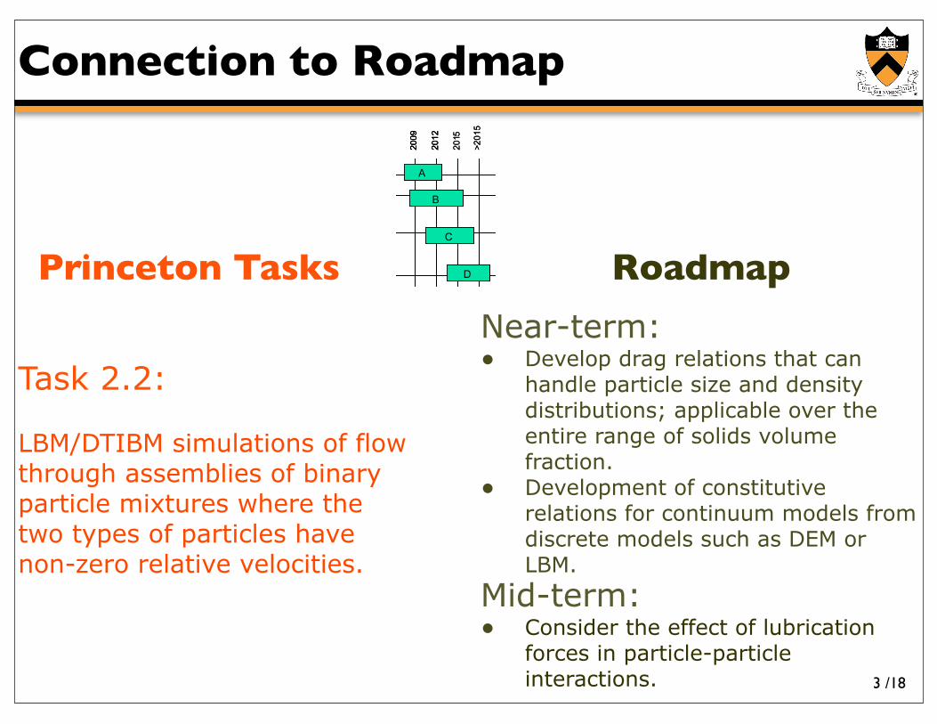
Connection to Roadmap
Princeton Tasks Roadmap
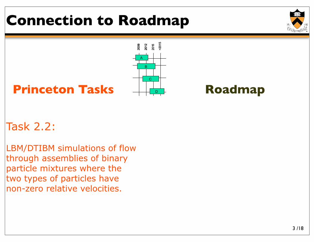
Task 2.2:
LBM/DTIBM simulations of flow through assemblies of binary particle mixtures where the two types of particles have non-zero relative velocities.
!"#$%&"' "( )*+,-'&.%/ 0+"1 2/%/.#3&4 5*(/ 6784 9::6
9:
2015
>2015
1. Fundamental aspects of stress and flow fields in dense
particulate systems.
2. Definition of material properties on relevant scales, along with
efficient ways to represent properties in models and establish
standards for material property measurements.
3. Given the practical need for continuum modeling capability,
identify the inherent limitations and how to proceed forward, e.g.,
hybrid models that connect with finer scale models (DNS, DEM,finite element, stochastic, etc.) for finer resolution.
4. Size-scaling and process control (particle / unit-op / processing
system) is critical to industrial applications.
2009
2012
A
B
C
D
2015
>2015
1. Fundamental aspects of stress and flow fields in dense
particulate systems.
2. Definition of material properties on relevant scales, along with
efficient ways to represent properties in models and establish
standards for material property measurements.
3. Given the practical need for continuum modeling capability,
identify the inherent limitations and how to proceed forward, e.g.,
hybrid models that connect with finer scale models (DNS, DEM,finite element, stochastic, etc.) for finer resolution.
4. Size-scaling and process control (particle / unit-op / processing
system) is critical to industrial applications.
2009
2012
A
B
C
D
1. Fundamental aspects of stress and flow fields in dense
particulate systems.
2. Definition of material properties on relevant scales, along with
efficient ways to represent properties in models and establish
standards for material property measurements.
3. Given the practical need for continuum modeling capability,
identify the inherent limitations and how to proceed forward, e.g.,
hybrid models that connect with finer scale models (DNS, DEM,finite element, stochastic, etc.) for finer resolution.
4. Size-scaling and process control (particle / unit-op / processing
system) is critical to industrial applications.
2009
2012
A
B
C
D
!"#$%& '('( ;,#.,/<-3 ,-=/+-(/ >"# .??#/%%-(< $/@ ,"'-3.+ .#/.% #/+.,/? ,"?/(%/ '&.%/ >+"1%A B+"3$ C -% '#-=.#-+@ 3"(3/#(/? 1-,& ,&/ -%%*/% -(
D.E+/ FAFG B #/>/#% ," -%%*/% -( D.E+/ FA9G H #/>/#% ," D.E+/ FAI .(? J#/>/#% ," D.E+/ FAKAA
! !"#$ %&'( ")* +&,-./ %01"'(/2
3
/18
Connection to Roadmap
Princeton Tasks Roadmap
Task 2.2:
LBM/DTIBM simulations of flow through assemblies of binary particle mixtures where the two types of particles have non-zero relative velocities.
Near-term:• Develop drag relations that can
handle particle size and density distributions; applicable over the entire range of solids volume fraction.
• Development of constitutive relations for continuum models from discrete models such as DEM or LBM.
Mid-term:• Consider the effect of lubrication
forces in particle-particle interactions.
!"#$%&"' "( )*+,-'&.%/ 0+"1 2/%/.#3&4 5*(/ 6784 9::6
9:
2015
>2015
1. Fundamental aspects of stress and flow fields in dense
particulate systems.
2. Definition of material properties on relevant scales, along with
efficient ways to represent properties in models and establish
standards for material property measurements.
3. Given the practical need for continuum modeling capability,
identify the inherent limitations and how to proceed forward, e.g.,
hybrid models that connect with finer scale models (DNS, DEM,finite element, stochastic, etc.) for finer resolution.
4. Size-scaling and process control (particle / unit-op / processing
system) is critical to industrial applications.
2009
2012
A
B
C
D
2015
>2015
1. Fundamental aspects of stress and flow fields in dense
particulate systems.
2. Definition of material properties on relevant scales, along with
efficient ways to represent properties in models and establish
standards for material property measurements.
3. Given the practical need for continuum modeling capability,
identify the inherent limitations and how to proceed forward, e.g.,
hybrid models that connect with finer scale models (DNS, DEM,finite element, stochastic, etc.) for finer resolution.
4. Size-scaling and process control (particle / unit-op / processing
system) is critical to industrial applications.
2009
2012
A
B
C
D
1. Fundamental aspects of stress and flow fields in dense
particulate systems.
2. Definition of material properties on relevant scales, along with
efficient ways to represent properties in models and establish
standards for material property measurements.
3. Given the practical need for continuum modeling capability,
identify the inherent limitations and how to proceed forward, e.g.,
hybrid models that connect with finer scale models (DNS, DEM,finite element, stochastic, etc.) for finer resolution.
4. Size-scaling and process control (particle / unit-op / processing
system) is critical to industrial applications.
2009
2012
A
B
C
D
!"#$%& '('( ;,#.,/<-3 ,-=/+-(/ >"# .??#/%%-(< $/@ ,"'-3.+ .#/.% #/+.,/? ,"?/(%/ '&.%/ >+"1%A B+"3$ C -% '#-=.#-+@ 3"(3/#(/? 1-,& ,&/ -%%*/% -(
D.E+/ FAFG B #/>/#% ," -%%*/% -( D.E+/ FA9G H #/>/#% ," D.E+/ FAI .(? J#/>/#% ," D.E+/ FAKAA
! !"#$ %&'( ")* +&,-./ %01"'(/2
3
/18
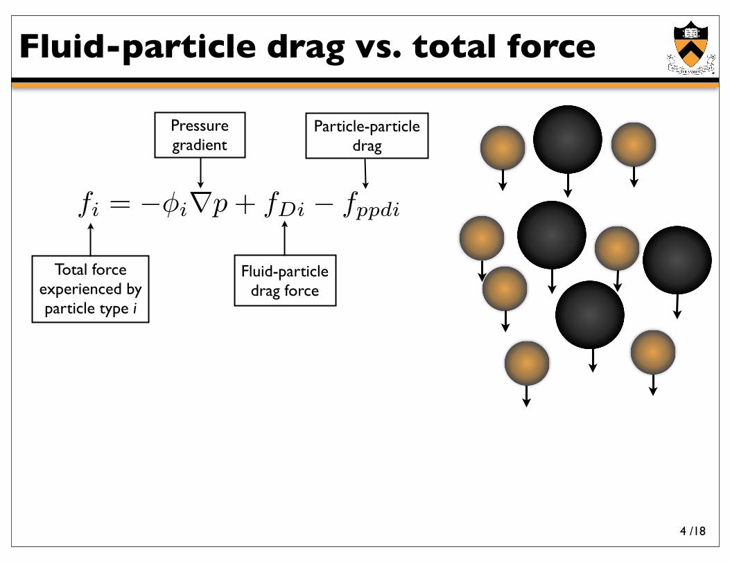
Particle-particle drag
Total force experienced by particle type i
Pressure gradient
Fluid-particle drag force
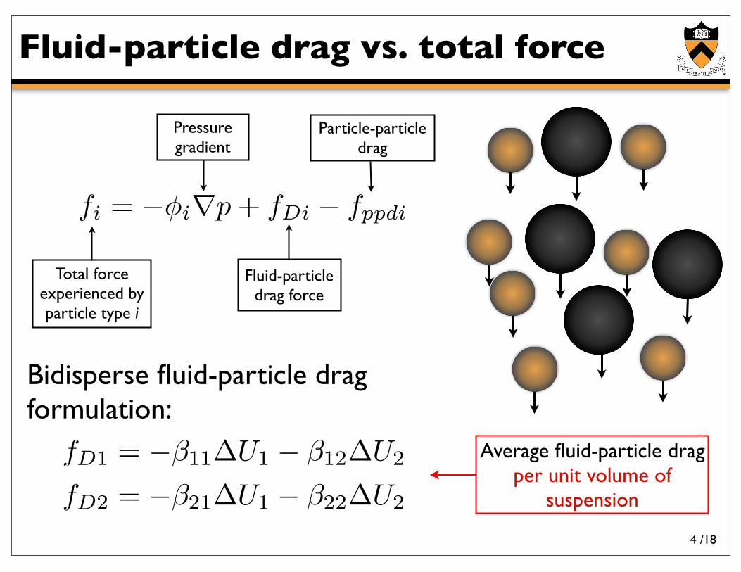
fi = !!i"p + fDi ! fppdi
Fluid-particle drag vs. total force
4
/18
Bidisperse fluid-particle drag formulation:
Particle-particle drag
Total force experienced by particle type i
Pressure gradient
Fluid-particle drag force
fi = !!i"p + fDi ! fppdi
fD1 = !!11!U1 ! !12!U2
fD2 = !!21!U1 ! !22!U2
Average fluid-particle drag per unit volume of
suspension
Fluid-particle drag vs. total force
4
/18
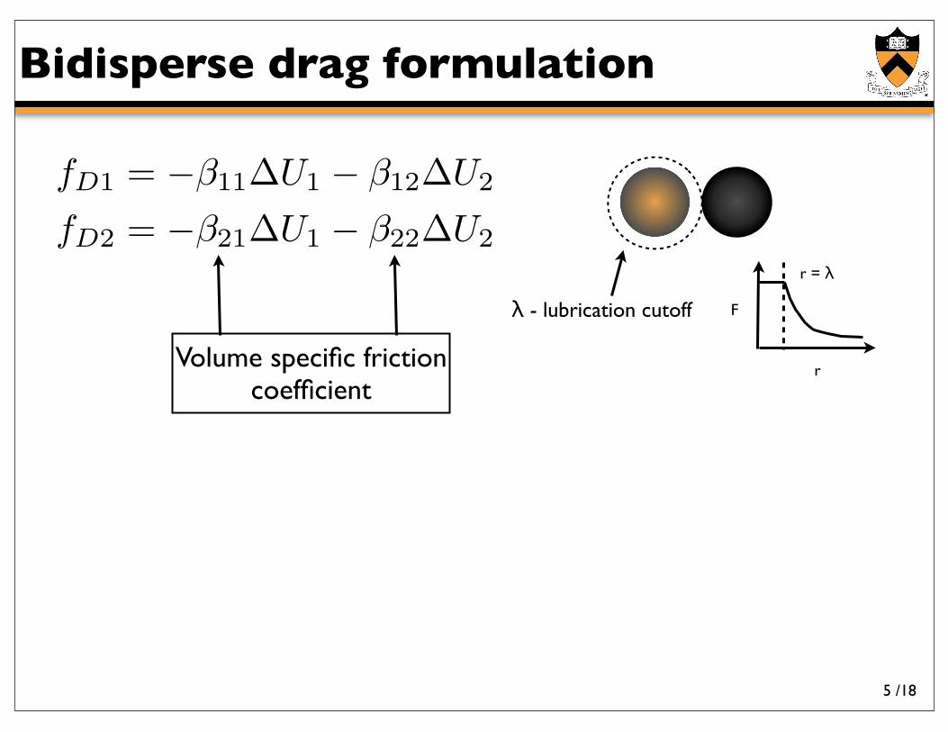
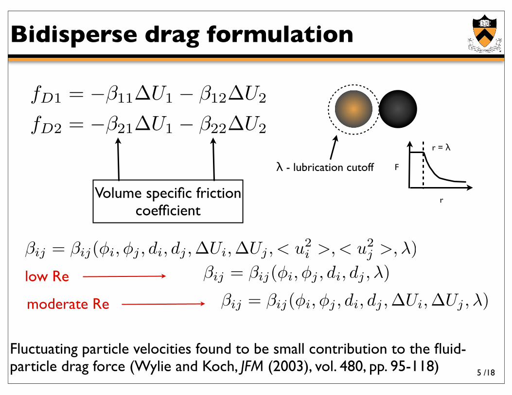
Bidisperse drag formulation
fD1 = !!11!U1 ! !12!U2
fD2 = !!21!U1 ! !22!U2
Volume specific friction coefficient
λ - lubrication cutoff
r = λ
r
F
5
/18
Bidisperse drag formulation
fD1 = !!11!U1 ! !12!U2
fD2 = !!21!U1 ! !22!U2
Volume specific friction coefficient
low Re
moderate Re
λ - lubrication cutoff
r = λ
r
F
Fluctuating particle velocities found to be small contribution to the fluid-particle drag force (Wylie and Koch, JFM (2003), vol. 480, pp. 95-118) 5
!ij = !ij("i, "j , di, dj ,!Ui,!Uj , < u2i >, < u2
j >, #)!ij = !ij("i, "j , di, dj , #)
!ij = !ij("i, "j , di, dj ,!Ui,!Uj , #)
/18
Simulation Procedures
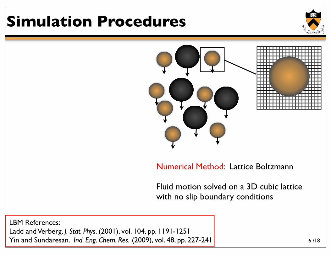
Numerical Method: Lattice Boltzmann
Fluid motion solved on a 3D cubic lattice with no slip boundary conditions
LBM References:Ladd and Verberg, J. Stat. Phys. (2001), vol. 104, pp. 1191-1251Yin and Sundaresan. Ind. Eng. Chem. Res. (2009), vol. 48, pp. 227-241 6
/18
Simulation Procedures
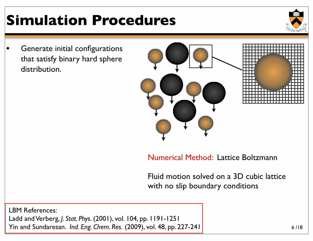
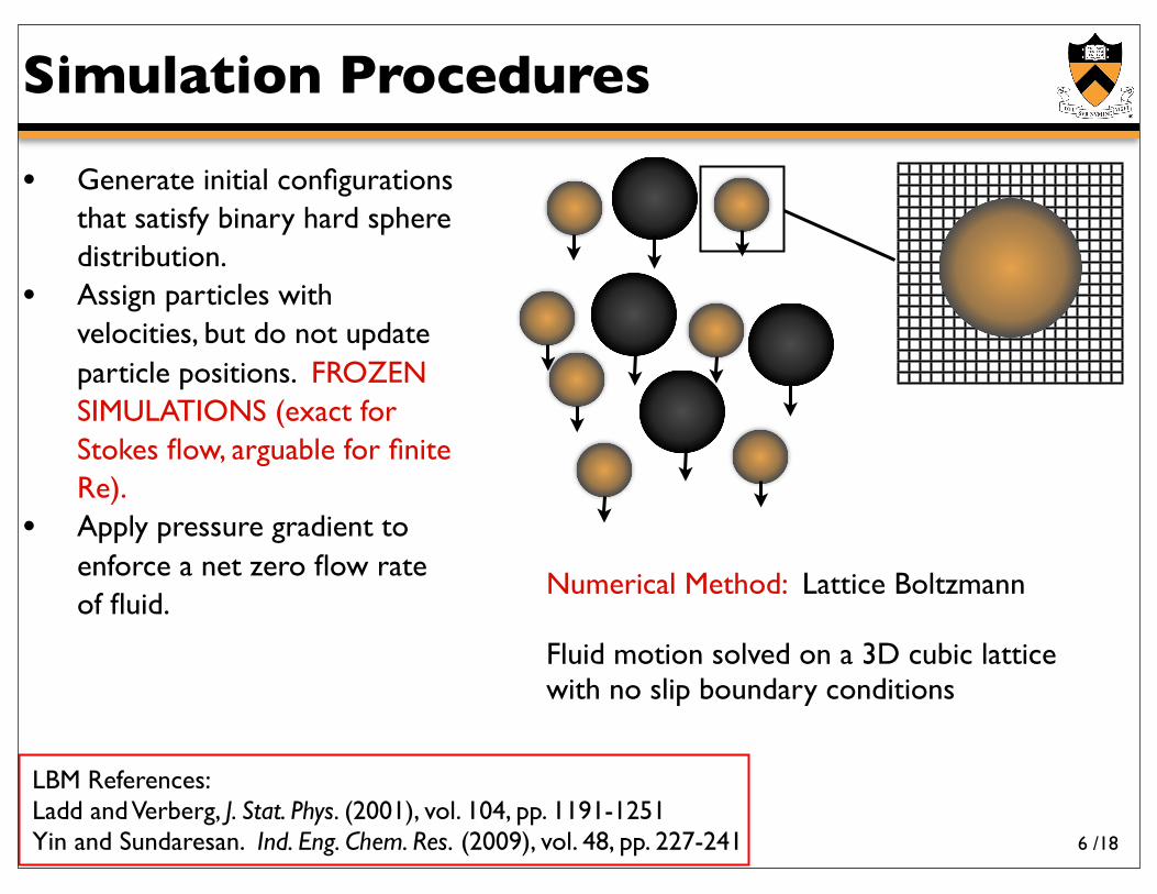
• Generate initial configurations that satisfy binary hard sphere distribution.
Numerical Method: Lattice Boltzmann
Fluid motion solved on a 3D cubic lattice with no slip boundary conditions
LBM References:Ladd and Verberg, J. Stat. Phys. (2001), vol. 104, pp. 1191-1251Yin and Sundaresan. Ind. Eng. Chem. Res. (2009), vol. 48, pp. 227-241 6
/18
Simulation Procedures
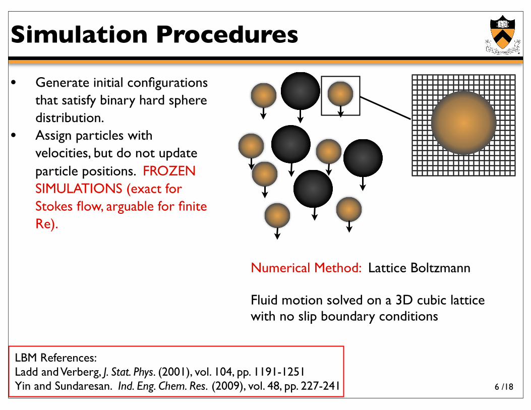
• Generate initial configurations that satisfy binary hard sphere distribution.
• Assign particles with velocities, but do not update particle positions. FROZEN SIMULATIONS (exact for Stokes flow, arguable for finite Re).
Numerical Method: Lattice Boltzmann
Fluid motion solved on a 3D cubic lattice with no slip boundary conditions
LBM References:Ladd and Verberg, J. Stat. Phys. (2001), vol. 104, pp. 1191-1251Yin and Sundaresan. Ind. Eng. Chem. Res. (2009), vol. 48, pp. 227-241 6
/18
Simulation Procedures
• Generate initial configurations that satisfy binary hard sphere distribution.
• Assign particles with velocities, but do not update particle positions. FROZEN SIMULATIONS (exact for Stokes flow, arguable for finite Re).
• Apply pressure gradient to enforce a net zero flow rate of fluid.
Numerical Method: Lattice Boltzmann
Fluid motion solved on a 3D cubic lattice with no slip boundary conditions
LBM References:Ladd and Verberg, J. Stat. Phys. (2001), vol. 104, pp. 1191-1251Yin and Sundaresan. Ind. Eng. Chem. Res. (2009), vol. 48, pp. 227-241 6
/18
Simulation Procedures
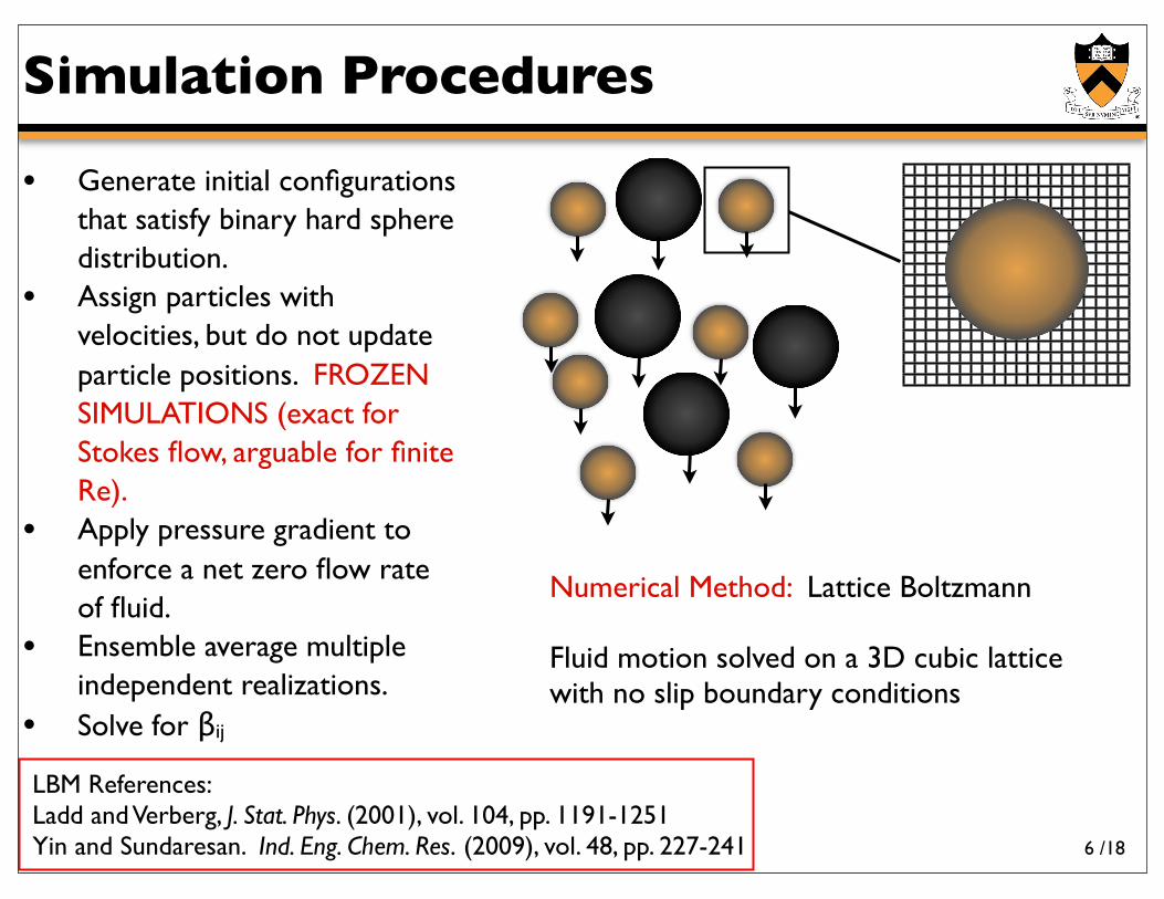
• Generate initial configurations that satisfy binary hard sphere distribution.
• Assign particles with velocities, but do not update particle positions. FROZEN SIMULATIONS (exact for Stokes flow, arguable for finite Re).
• Apply pressure gradient to enforce a net zero flow rate of fluid.
• Ensemble average multiple independent realizations.
• Solve for βij
Numerical Method: Lattice Boltzmann
Fluid motion solved on a 3D cubic lattice with no slip boundary conditions
LBM References:Ladd and Verberg, J. Stat. Phys. (2001), vol. 104, pp. 1191-1251Yin and Sundaresan. Ind. Eng. Chem. Res. (2009), vol. 48, pp. 227-241 6
/18
Low Re bidisperse systems
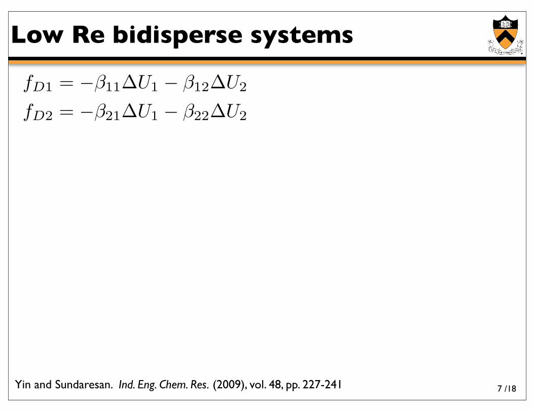
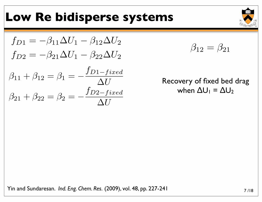
fD1 = !!11!U1 ! !12!U2
fD2 = !!21!U1 ! !22!U2
Yin and Sundaresan. Ind. Eng. Chem. Res. (2009), vol. 48, pp. 227-241 7
/18
Low Re bidisperse systems
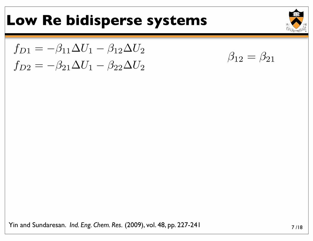
fD1 = !!11!U1 ! !12!U2
fD2 = !!21!U1 ! !22!U2!12 = !21
Yin and Sundaresan. Ind. Eng. Chem. Res. (2009), vol. 48, pp. 227-241 7
/18
Low Re bidisperse systems
fD1 = !!11!U1 ! !12!U2
fD2 = !!21!U1 ! !22!U2!12 = !21
!11 + !12 = !1 = !fD1!fixed
!U
!21 + !22 = !2 = !fD2!fixed
!U
Recovery of fixed bed drag when ΔU1 = ΔU2
Yin and Sundaresan. Ind. Eng. Chem. Res. (2009), vol. 48, pp. 227-241 7
/18
Low Re bidisperse systems
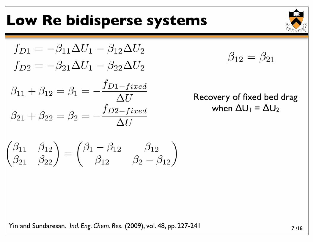
fD1 = !!11!U1 ! !12!U2
fD2 = !!21!U1 ! !22!U2!12 = !21
!11 + !12 = !1 = !fD1!fixed
!U
!21 + !22 = !2 = !fD2!fixed
!U
!!11 !12
!21 !22
"=
!!1 ! !12 !12
!12 !2 ! !12
"
Recovery of fixed bed drag when ΔU1 = ΔU2
Yin and Sundaresan. Ind. Eng. Chem. Res. (2009), vol. 48, pp. 227-241 7
/18
Low Re bidisperse systems
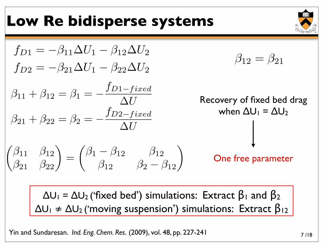
fD1 = !!11!U1 ! !12!U2
fD2 = !!21!U1 ! !22!U2!12 = !21
!11 + !12 = !1 = !fD1!fixed
!U
!21 + !22 = !2 = !fD2!fixed
!U
!!11 !12
!21 !22
"=
!!1 ! !12 !12
!12 !2 ! !12
"
Recovery of fixed bed drag when ΔU1 = ΔU2
One free parameter
ΔU1 = ΔU2 (‘fixed bed’) simulations: Extract β1 and β2
ΔU1 ≠ ΔU2 (‘moving suspension’) simulations: Extract β12
Yin and Sundaresan. Ind. Eng. Chem. Res. (2009), vol. 48, pp. 227-241 7
/18
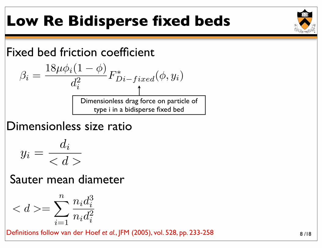
Low Re Bidisperse fixed beds
Definitions follow van der Hoef et al., JFM (2005), vol. 528, pp. 233-258
Sauter mean diameter
< d >=n!
i=1
nid3i
nid2i
Dimensionless size ratio
yi =di
< d >
!i =18µ"i(1! ")
d2i
F !Di"fixed(", yi)
Fixed bed friction coefficient
Dimensionless drag force on particle of type i in a bidisperse fixed bed
8
/18
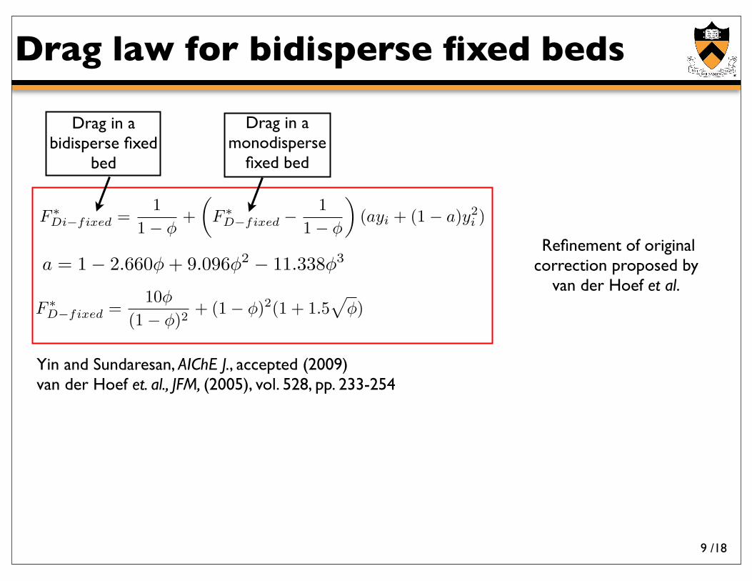
Drag law for bidisperse fixed beds
Yin and Sundaresan, AIChE J., accepted (2009)van der Hoef et. al., JFM, (2005), vol. 528, pp. 233-254
Refinement of original correction proposed by
van der Hoef et al.
9
F !D"fixed =
10!
(1! !)2+ (1! !)2(1 + 1.5
!!)
F !Di"fixed =
11! !
+!
F !D"fixed !
11! !
"(ayi + (1! a)y2
i )
Drag in a bidisperse fixed
bed
Drag in a monodisperse
fixed bed
a = 1! 2.660! + 9.096!2 ! 11.338!3
/18
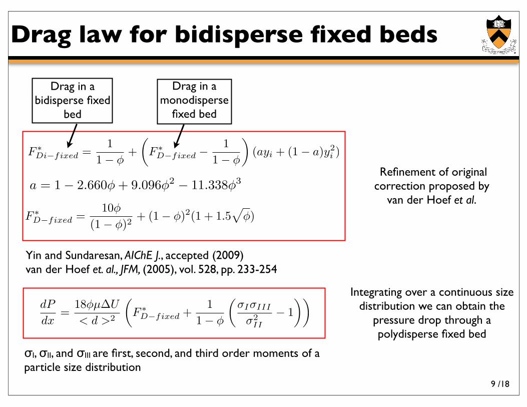
Drag law for bidisperse fixed beds
dP
dx=
18!µ!U
< d >2
!F !
D"fixed +1
1! !
!"I"III
"2II
! 1"" Integrating over a continuous size
distribution we can obtain the pressure drop through a polydisperse fixed bed
σI, σII, and σIII are first, second, and third order moments of a particle size distribution
Yin and Sundaresan, AIChE J., accepted (2009)van der Hoef et. al., JFM, (2005), vol. 528, pp. 233-254
Refinement of original correction proposed by
van der Hoef et al.
9
F !D"fixed =
10!
(1! !)2+ (1! !)2(1 + 1.5
!!)
F !Di"fixed =
11! !
+!
F !D"fixed !
11! !
"(ayi + (1! a)y2
i )
Drag in a bidisperse fixed
bed
Drag in a monodisperse
fixed bed
a = 1! 2.660! + 9.096!2 ! 11.338!3
/18
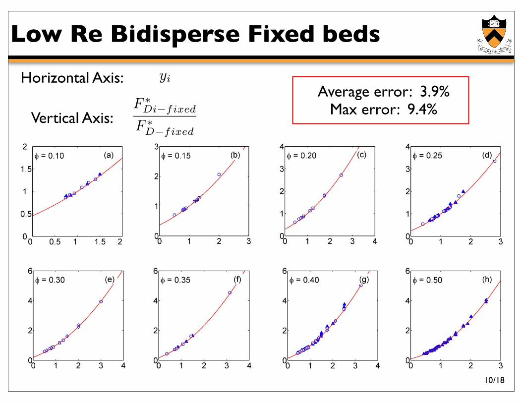
Low Re Bidisperse Fixed beds
Horizontal Axis:
Vertical Axis:F !
Di"fixed
F !D"fixed
yi
Average error: 3.9%Max error: 9.4%
10
/18
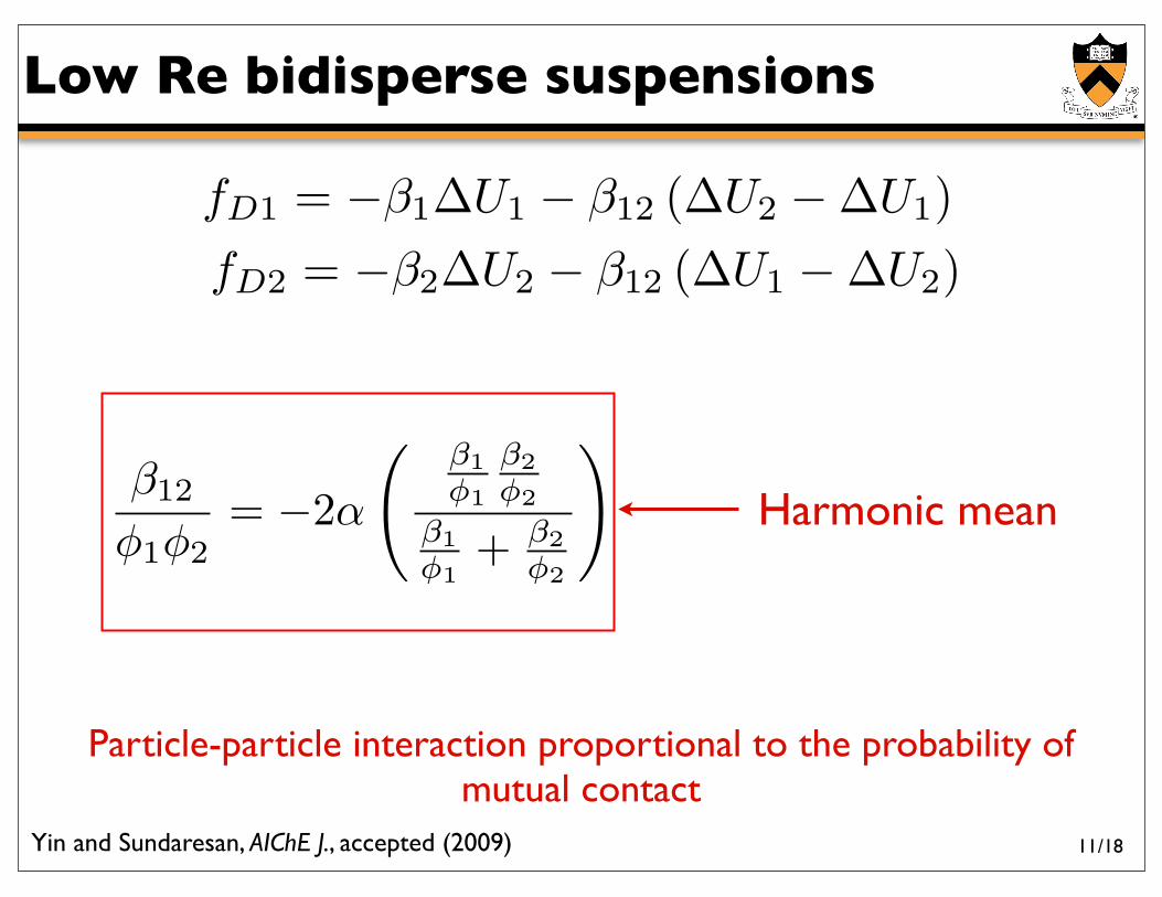
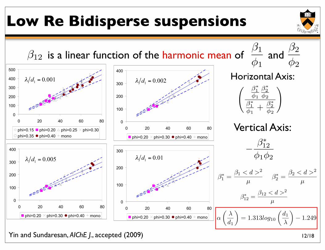
Low Re bidisperse suspensions
Particle-particle interaction proportional to the probability of mutual contact
!12
"1"2= !2#
!!1"1
!2"2
!1"1
+ !2"2
"Harmonic mean
Yin and Sundaresan, AIChE J., accepted (2009)
fD1 = !!1!U1 ! !12 (!U2 !!U1)fD2 = !!2!U2 ! !12 (!U1 !!U2)
11
/18
Low Re Bidisperse suspensions
0
100
200
300
400
500
0 20 40 60 80
phi=0.15 phi=0.20 phi=0.25 phi=0.30phi=0.35 phi=0.40 mono
0
100
200
300
400
0 20 40 60 80
phi=0.20 phi=0.30 phi=0.40 mono
0
100
200
300
400
0 20 40 60 80
phi=0.20 phi=0.30 phi=0.40 mono
0
100
200
300
0 20 40 60 80
phi=0.20 phi=0.30 phi=0.40 mono
001.01 =dλ 002.01 =dλ
005.01 =dλ 01.01 =dλ
! !!1"1
!!2"2
!!1"1
+ !!2"2
"Horizontal Axis:
Vertical Axis:
! !!12
"1"2
!!12 =
!12 < d >2
µ
!!1 =
!1 < d >2
µ!!
2 =!2 < d >2
µ
!
!"
d1
"= 1.313log10
!d1
"
"! 1.249
is a linear function of the harmonic mean of and!12!1
"1
!2
"2
12Yin and Sundaresan, AIChE J., accepted (2009)
/18
Simulations at finite Re
Frozen suspension at finite Re Moving suspension at finite Re
• Inertial lag prevents fluid from adapting to particle motion
instantaneously
13
/18
Simulations at finite Re
Frozen suspension at finite Re
• Fluid adapts instantaneously to particle motion
Moving suspension at finite Re
• Inertial lag prevents fluid from adapting to particle motion
instantaneously
13

/18
Simulations at finite Re
Frozen suspension at finite Re
• Fluid adapts instantaneously to particle motion
Moving suspension at finite Re
• Inertial lag prevents fluid from adapting to particle motion
instantaneously
13
/18
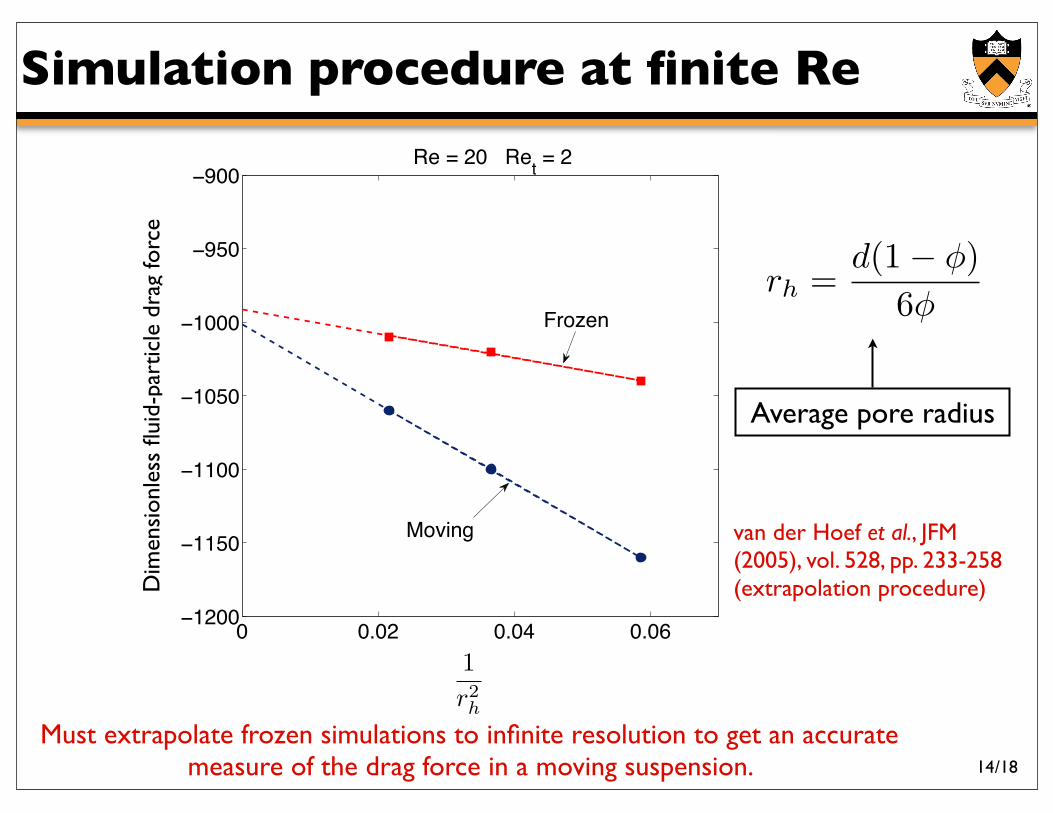
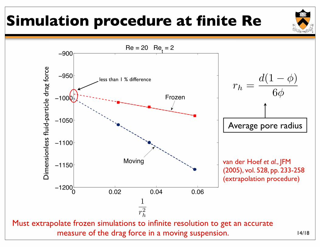
Simulation procedure at finite Re
Must extrapolate frozen simulations to infinite resolution to get an accurate measure of the drag force in a moving suspension.
Dim
ensi
onle
ss fl
uid-
part
icle
dra
g fo
rce
0 0.02 0.04 0.06−1200
−1150
−1100
−1050
−1000
−950
−900Re = 20 Ret = 2
Moving
Frozen
1r2h
van der Hoef et al., JFM (2005), vol. 528, pp. 233-258 (extrapolation procedure)
Average pore radius
rh =d(1! !)
6!
14
/18
Simulation procedure at finite Re
Must extrapolate frozen simulations to infinite resolution to get an accurate measure of the drag force in a moving suspension.
Dim
ensi
onle
ss fl
uid-
part
icle
dra
g fo
rce
0 0.02 0.04 0.06−1200
−1150
−1100
−1050
−1000
−950
−900Re = 20 Ret = 2
Moving
Frozen
1r2h
van der Hoef et al., JFM (2005), vol. 528, pp. 233-258 (extrapolation procedure)
less than 1 % difference
Average pore radius
rh =d(1! !)
6!
14
/18
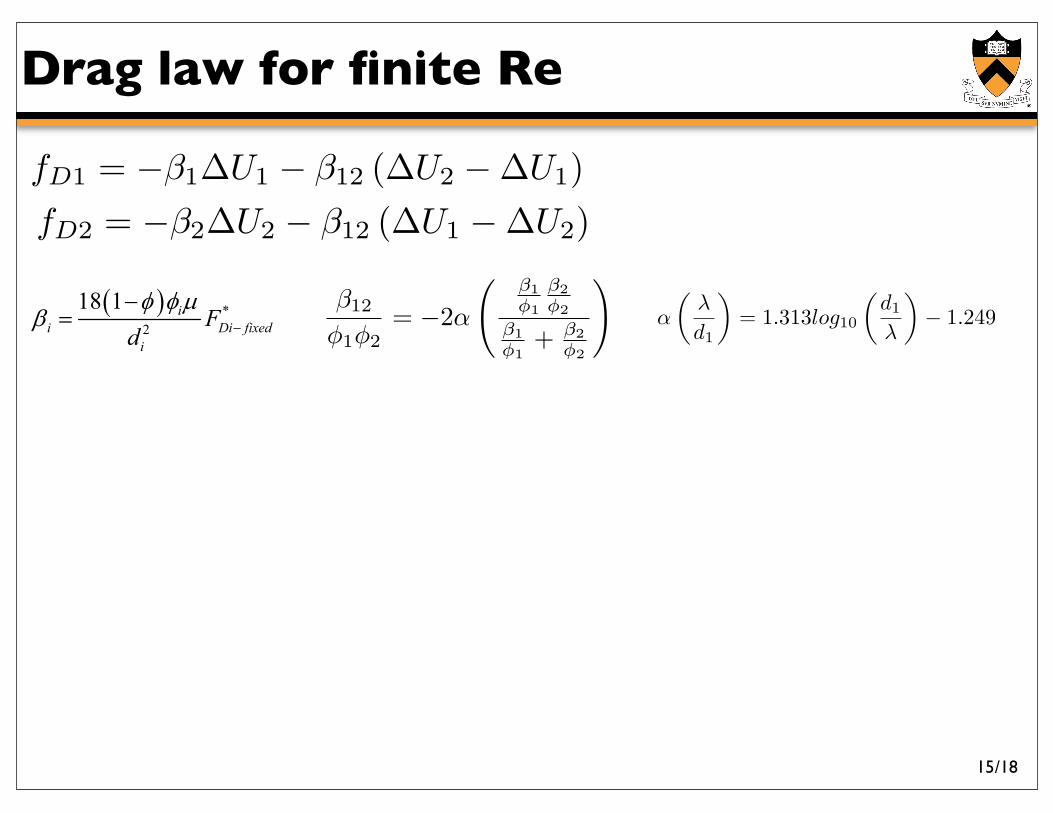
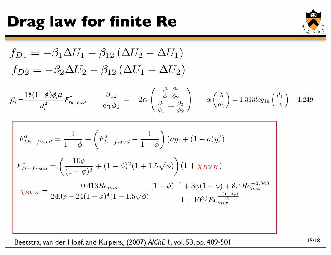
Drag law for finite Re
fD1 = !!1!U1 ! !12 (!U2 !!U1)fD2 = !!2!U2 ! !12 (!U1 !!U2)
!12
"1"2= !2#
!!1"1
!2"2
!1"1
+ !2"2
"!
!"
d1
"= 1.313log10
!d1
"
"! 1.249
Fluid-particle drag relation for inertial, bidisperse, gas-solid
suspensions in relative motion
The fluid-particle drag in a bidisperse suspension in the high Stokes number limit
can be expressed in the following way:
1 11 1 12
2 21 1 22
D
D
2
2
f U U
f U U
! !
! !
" # $ # $
" # $ # $ (1)
where Dif is the fluid-particle drag force on particles of type i per unit volume
suspension, is the relative velocity between particles of type i and the fluid, and iU$
ij! represents the volume specific friction coefficient on particles of type i due to the
motion of particles of type j.
In the limit of a fixed bed, 1U U2$ " $ , the drag relationship given by Eqn. (1) to
be simplified in the following way:
% &
% &
1 1 12 1 12
2 21 1 2 21
D
D
2
2
f U U
f U U
! ! !
! ! !
" # # $ # $
" # $ # # $ (2)
where
% & *
2
18 1 i
i
i
Fd
' ' (! #
#" Di fixed . (3)
In Eqn. (3) i! is the fixed bed friction coefficient of a particle of type i per unit volume,
' is the total volume fraction, i' is the volume fraction of species i,( is the fluid
viscosity, is the diameter of a particle of type i, and id *
Di fixedF # is the dimensionless fluid-
particle drag force on particles of type i in a bidisperse fixed bed ( *
Di f# ixedF is made
dimensionless by normalizing by the Stokes drag % &i Ud $#')( 13 ).
15
/18
Drag law for finite Re
fD1 = !!1!U1 ! !12 (!U2 !!U1)fD2 = !!2!U2 ! !12 (!U1 !!U2)
!12
"1"2= !2#
!!1"1
!2"2
!1"1
+ !2"2
"!
!"
d1
"= 1.313log10
!d1
"
"! 1.249
Fluid-particle drag relation for inertial, bidisperse, gas-solid
suspensions in relative motion
The fluid-particle drag in a bidisperse suspension in the high Stokes number limit
can be expressed in the following way:
1 11 1 12
2 21 1 22
D
D
2
2
f U U
f U U
! !
! !
" # $ # $
" # $ # $ (1)
where Dif is the fluid-particle drag force on particles of type i per unit volume
suspension, is the relative velocity between particles of type i and the fluid, and iU$
ij! represents the volume specific friction coefficient on particles of type i due to the
motion of particles of type j.
In the limit of a fixed bed, 1U U2$ " $ , the drag relationship given by Eqn. (1) to
be simplified in the following way:
% &
% &
1 1 12 1 12
2 21 1 2 21
D
D
2
2
f U U
f U U
! ! !
! ! !
" # # $ # $
" # $ # # $ (2)
where
% & *
2
18 1 i
i
i
Fd
' ' (! #
#" Di fixed . (3)
In Eqn. (3) i! is the fixed bed friction coefficient of a particle of type i per unit volume,
' is the total volume fraction, i' is the volume fraction of species i,( is the fluid
viscosity, is the diameter of a particle of type i, and id *
Di fixedF # is the dimensionless fluid-
particle drag force on particles of type i in a bidisperse fixed bed ( *
Di f# ixedF is made
dimensionless by normalizing by the Stokes drag % &i Ud $#')( 13 ).
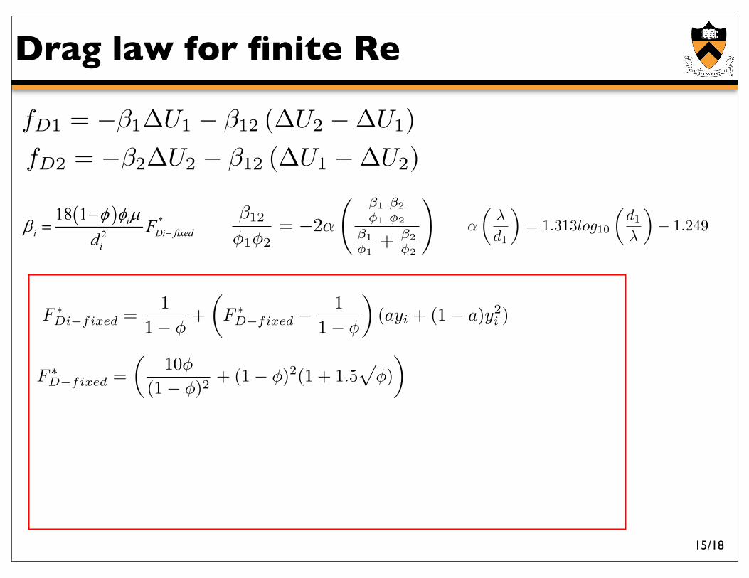
F !Di"fixed =
11! !
+!
F !D"fixed !
11! !
"(ayi + (1! a)y2
i )
15
F !D"fixed =
!10!
(1! !)2+ (1! !)2(1 + 1.5
"!)
#
/18
Drag law for finite Re
fD1 = !!1!U1 ! !12 (!U2 !!U1)fD2 = !!2!U2 ! !12 (!U1 !!U2)
!12
"1"2= !2#
!!1"1
!2"2
!1"1
+ !2"2
"!
!"
d1
"= 1.313log10
!d1
"
"! 1.249
Fluid-particle drag relation for inertial, bidisperse, gas-solid
suspensions in relative motion
The fluid-particle drag in a bidisperse suspension in the high Stokes number limit
can be expressed in the following way:
1 11 1 12
2 21 1 22
D
D
2
2
f U U
f U U
! !
! !
" # $ # $
" # $ # $ (1)
where Dif is the fluid-particle drag force on particles of type i per unit volume
suspension, is the relative velocity between particles of type i and the fluid, and iU$
ij! represents the volume specific friction coefficient on particles of type i due to the
motion of particles of type j.
In the limit of a fixed bed, 1U U2$ " $ , the drag relationship given by Eqn. (1) to
be simplified in the following way:
% &
% &
1 1 12 1 12
2 21 1 2 21
D
D
2
2
f U U
f U U
! ! !
! ! !
" # # $ # $
" # $ # # $ (2)
where
% & *
2
18 1 i
i
i
Fd
' ' (! #
#" Di fixed . (3)
In Eqn. (3) i! is the fixed bed friction coefficient of a particle of type i per unit volume,
' is the total volume fraction, i' is the volume fraction of species i,( is the fluid
viscosity, is the diameter of a particle of type i, and id *
Di fixedF # is the dimensionless fluid-
particle drag force on particles of type i in a bidisperse fixed bed ( *
Di f# ixedF is made
dimensionless by normalizing by the Stokes drag % &i Ud $#')( 13 ).
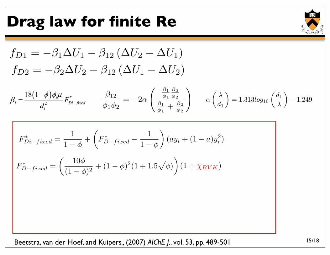
Beetstra, van der Hoef, and Kuipers., (2007) AIChE J., vol. 53, pp. 489-501
F !Di"fixed =
11! !
+!
F !D"fixed !
11! !
"(ayi + (1! a)y2
i )
15
F !D"fixed =
!10!
(1! !)2+ (1! !)2(1 + 1.5
"!)
#(1 + !BV K)
/18
Drag law for finite Re
fD1 = !!1!U1 ! !12 (!U2 !!U1)fD2 = !!2!U2 ! !12 (!U1 !!U2)
!12
"1"2= !2#
!!1"1
!2"2
!1"1
+ !2"2
"!
!"
d1
"= 1.313log10
!d1
"
"! 1.249
Fluid-particle drag relation for inertial, bidisperse, gas-solid
suspensions in relative motion
The fluid-particle drag in a bidisperse suspension in the high Stokes number limit
can be expressed in the following way:
1 11 1 12
2 21 1 22
D
D
2
2
f U U
f U U
! !
! !
" # $ # $
" # $ # $ (1)
where Dif is the fluid-particle drag force on particles of type i per unit volume
suspension, is the relative velocity between particles of type i and the fluid, and iU$
ij! represents the volume specific friction coefficient on particles of type i due to the
motion of particles of type j.
In the limit of a fixed bed, 1U U2$ " $ , the drag relationship given by Eqn. (1) to
be simplified in the following way:
% &
% &
1 1 12 1 12
2 21 1 2 21
D
D
2
2
f U U
f U U
! ! !
! ! !
" # # $ # $
" # $ # # $ (2)
where
% & *
2
18 1 i
i
i
Fd
' ' (! #
#" Di fixed . (3)
In Eqn. (3) i! is the fixed bed friction coefficient of a particle of type i per unit volume,
' is the total volume fraction, i' is the volume fraction of species i,( is the fluid
viscosity, is the diameter of a particle of type i, and id *
Di fixedF # is the dimensionless fluid-
particle drag force on particles of type i in a bidisperse fixed bed ( *
Di f# ixedF is made
dimensionless by normalizing by the Stokes drag % &i Ud $#')( 13 ).
Beetstra, van der Hoef, and Kuipers., (2007) AIChE J., vol. 53, pp. 489-501
F !Di"fixed =
11! !
+!
F !D"fixed !
11! !
"(ayi + (1! a)y2
i )
!BV K =0.413Remix
240" + 24(1! ")4(1 + 1.5"
")(1! ")!1 + 3"(1! ") + 8.4Re!0.343
mix
1 + 103!Re!(1+4!)
2mix
15
F !D"fixed =
!10!
(1! !)2+ (1! !)2(1 + 1.5
"!)
#(1 + !BV K)
/18
Drag law for finite Re
fD1 = !!1!U1 ! !12 (!U2 !!U1)fD2 = !!2!U2 ! !12 (!U1 !!U2)
!12
"1"2= !2#
!!1"1
!2"2
!1"1
+ !2"2
"!
!"
d1
"= 1.313log10
!d1
"
"! 1.249
Fluid-particle drag relation for inertial, bidisperse, gas-solid
suspensions in relative motion
The fluid-particle drag in a bidisperse suspension in the high Stokes number limit
can be expressed in the following way:
1 11 1 12
2 21 1 22
D
D
2
2
f U U
f U U
! !
! !
" # $ # $
" # $ # $ (1)
where Dif is the fluid-particle drag force on particles of type i per unit volume
suspension, is the relative velocity between particles of type i and the fluid, and iU$
ij! represents the volume specific friction coefficient on particles of type i due to the
motion of particles of type j.
In the limit of a fixed bed, 1U U2$ " $ , the drag relationship given by Eqn. (1) to
be simplified in the following way:
% &
% &
1 1 12 1 12
2 21 1 2 21
D
D
2
2
f U U
f U U
! ! !
! ! !
" # # $ # $
" # $ # # $ (2)
where
% & *
2
18 1 i
i
i
Fd
' ' (! #
#" Di fixed . (3)
In Eqn. (3) i! is the fixed bed friction coefficient of a particle of type i per unit volume,
' is the total volume fraction, i' is the volume fraction of species i,( is the fluid
viscosity, is the diameter of a particle of type i, and id *
Di fixedF # is the dimensionless fluid-
particle drag force on particles of type i in a bidisperse fixed bed ( *
Di f# ixedF is made
dimensionless by normalizing by the Stokes drag % &i Ud $#')( 13 ).
Beetstra, van der Hoef, and Kuipers., (2007) AIChE J., vol. 53, pp. 489-501
F !Di"fixed =
11! !
+!
F !D"fixed !
11! !
"(ayi + (1! a)y2
i )
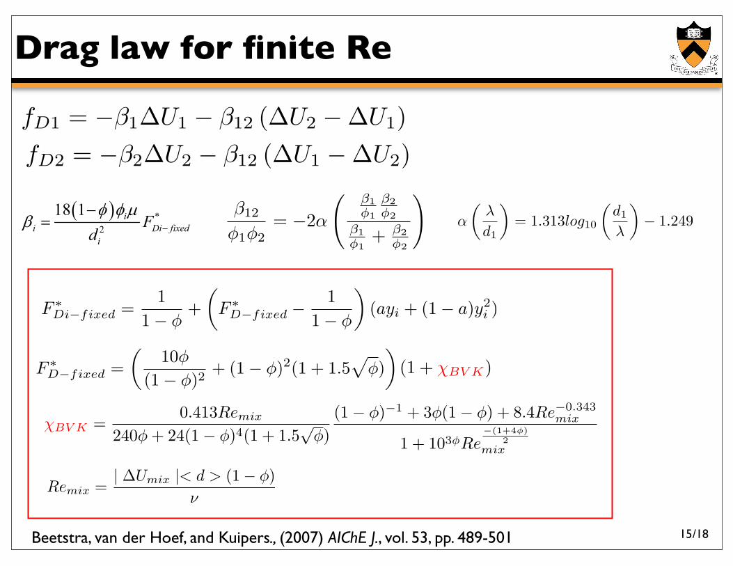
Remix =| !Umix |< d > (1! !)
"
!BV K =0.413Remix
240" + 24(1! ")4(1 + 1.5"
")(1! ")!1 + 3"(1! ") + 8.4Re!0.343
mix
1 + 103!Re!(1+4!)
2mix
15
F !D"fixed =
!10!
(1! !)2+ (1! !)2(1 + 1.5
"!)
#(1 + !BV K)
/18
Drag law for finite Re
fD1 = !!1!U1 ! !12 (!U2 !!U1)fD2 = !!2!U2 ! !12 (!U1 !!U2)
!12
"1"2= !2#
!!1"1
!2"2
!1"1
+ !2"2
"!
!"
d1
"= 1.313log10
!d1
"
"! 1.249
Fluid-particle drag relation for inertial, bidisperse, gas-solid
suspensions in relative motion
The fluid-particle drag in a bidisperse suspension in the high Stokes number limit
can be expressed in the following way:
1 11 1 12
2 21 1 22
D
D
2
2
f U U
f U U
! !
! !
" # $ # $
" # $ # $ (1)
where Dif is the fluid-particle drag force on particles of type i per unit volume
suspension, is the relative velocity between particles of type i and the fluid, and iU$
ij! represents the volume specific friction coefficient on particles of type i due to the
motion of particles of type j.
In the limit of a fixed bed, 1U U2$ " $ , the drag relationship given by Eqn. (1) to
be simplified in the following way:
% &
% &
1 1 12 1 12
2 21 1 2 21
D
D
2
2
f U U
f U U
! ! !
! ! !
" # # $ # $
" # $ # # $ (2)
where
% & *
2
18 1 i
i
i
Fd
' ' (! #
#" Di fixed . (3)
In Eqn. (3) i! is the fixed bed friction coefficient of a particle of type i per unit volume,
' is the total volume fraction, i' is the volume fraction of species i,( is the fluid
viscosity, is the diameter of a particle of type i, and id *
Di fixedF # is the dimensionless fluid-
particle drag force on particles of type i in a bidisperse fixed bed ( *
Di f# ixedF is made
dimensionless by normalizing by the Stokes drag % &i Ud $#')( 13 ).
Beetstra, van der Hoef, and Kuipers., (2007) AIChE J., vol. 53, pp. 489-501
F !Di"fixed =
11! !
+!
F !D"fixed !
11! !
"(ayi + (1! a)y2
i )
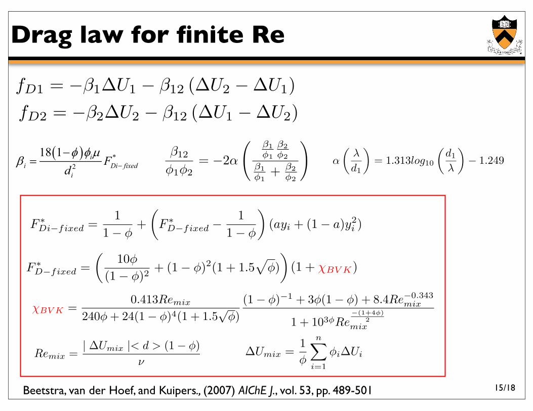
Remix =| !Umix |< d > (1! !)
"!Umix =
1!
n!
i=1
!i!Ui
!BV K =0.413Remix
240" + 24(1! ")4(1 + 1.5"
")(1! ")!1 + 3"(1! ") + 8.4Re!0.343
mix
1 + 103!Re!(1+4!)
2mix
15
F !D"fixed =
!10!
(1! !)2+ (1! !)2(1 + 1.5
"!)
#(1 + !BV K)
/18
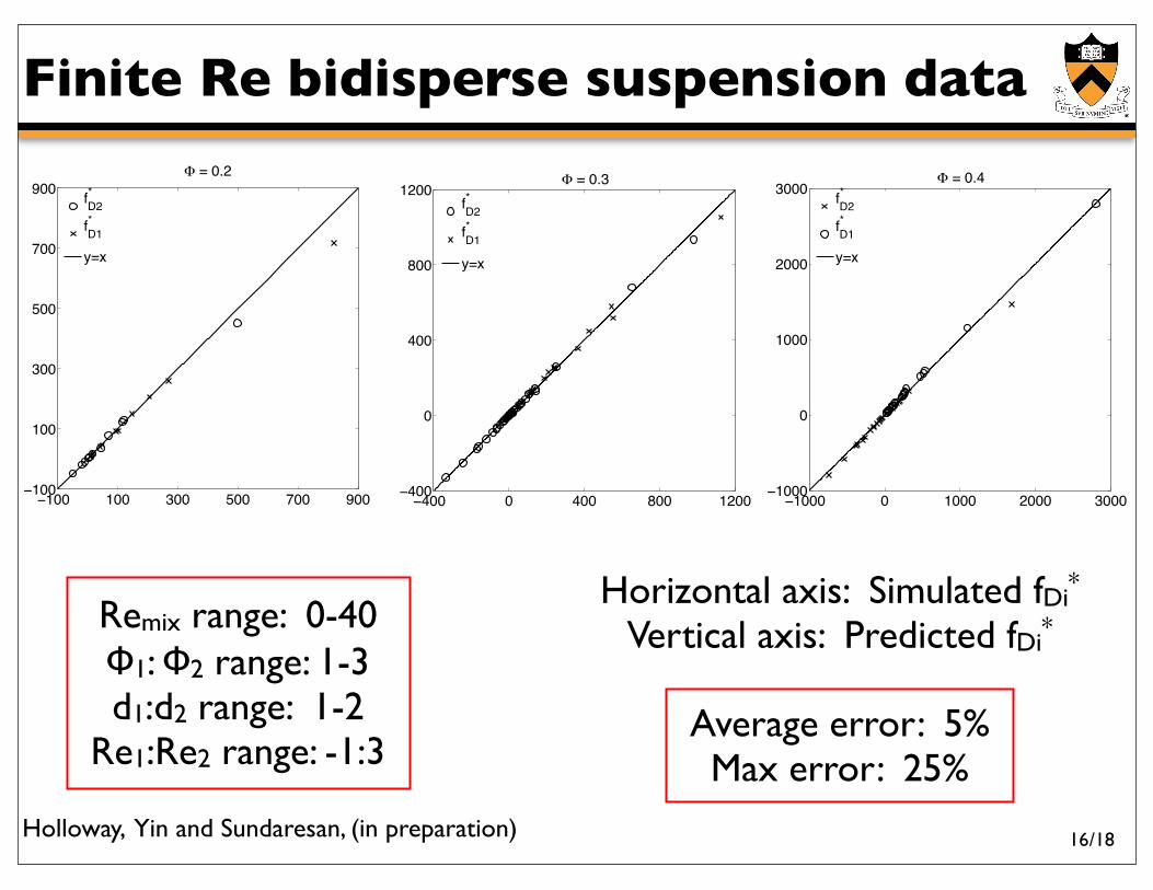
Finite Re bidisperse suspension data
Holloway, Yin and Sundaresan, (in preparation)
Remix range: 0-40Φ1: Φ2 range: 1-3d1:d2 range: 1-2
Re1:Re2 range: -1:3Average error: 5%Max error: 25%
Horizontal axis: Simulated fDi* Vertical axis: Predicted fDi*
−400 0 400 800 1200−400
0
400
800
1200
! = 0.3
fD2*
fD1*
y=x
−1000 0 1000 2000 3000−1000
0
1000
2000
3000! = 0.4
fD2*
fD1*
y=x
−100 100 300 500 700 900−100
100
300
500
700
900! = 0.2
fD2*
fD1*
y=x
16
/18
Looking ahead
• Combine LBM results at moderate Re together with IBM results from Subramaniam group at higher Re.
• Perform freely evolving bidisperse simulations to investigate particle-particle collisional interactions in sedimenting systems.
17
/18
Summary
• Fluid-particle drag relation developed that accurately predicts fluid-particle drag in Stokesian suspensions with particle-particle relative motion and size differences.
• Drag relation extended to account for moderate fluid inertia in bidisperse suspension flows.
Acknowledgements
• US Department of Energy• ExxonMobil Corporation• ACS Petroleum Research Fund
18