negative point mass singularities in general …bray/phd theses/robbins.pdfnegative point mass...
TRANSCRIPT
NEGATIVE POINT MASS SINGULARITIES IN
GENERAL RELATIVITY
by
Nicholas P. Robbins
Department of MathematicsDuke University
Date:Approved:
Hubert L. Bray, Advisor
Mark A. Stern
Paul A. Aspinwall
N. Ronen Plesser
Dissertation submitted in partial fulfillment of therequirements for the degree of Doctor of Philosophy
in the Department of Mathematicsin the Graduate School of
Duke University
2007
ABSTRACT
(Mathematics)
NEGATIVE POINT MASS SINGULARITIES IN
GENERAL RELATIVITY
by
Nicholas P. Robbins
Department of MathematicsDuke University
Date:Approved:
Hubert L. Bray, Advisor
Mark A. Stern
Paul A. Aspinwall
N. Ronen Plesser
An abstract of a dissertation submitted in partial fulfillment of therequirements for the degree of Doctor of Philosophy
in the Department of Mathematicsin the Graduate School of
Duke University
2007

Copyright c© 2007 by Nicholas P. Robbins
All rights reserved
Abstract
First we review the definition of a negative point mass singularity. Then we examine
the gravitational lensing effects of these singularities in isolation and with shear and
convergence from continuous matter. We review the Inverse Mean Curvature Flow
and use this flow to prove some new results about the mass of a singularity, the
ADM mass of the manifold, and the capacity of the singularity. We describe some
particular examples of these singularities that exhibit additional symmetries.
iv

Acknowledgements
I want to thank my thesis advisor, Professor Hubert Bray. Without your copious
support, advice, and encouragement throughout my thesis process this would not
have been possible.
Thanks also to the many faculty members who have helped me throughout my
career at Duke. Thanks to Professors Mark Stern, Paul Aspinwall and Ronen Plesser
for your extensive feedback during the thesis writing process. I want to thank Profes-
sor Stern in particular for the courses which formed the backbone of my coursework
at Duke. Thanks to Professor Tom Witelski for your helpful advice and support at
a difficult time in my graduate career.
I have had wonderful support for developing my teaching skills while at Duke.
Thanks to James Tomberg and Professor Jack Bookman in particular for your ex-
tensive support for my teaching and career, as well as Professor Lewis Blake for your
work supporting undergraduate instruction.
I also want to thank Professor Jennifer Hontz at Meredith College for allowing
me to see academic life outside of Duke University.
I want to thank all the departmental staff. In particular, thanks to Georgia Barns
and Shannon Holder for helping me over innumerable institutional hurdles.
I have had the pleasure of many meaningful friendships with the other graduate
students in the program. In particular I wish to thank my officemates Melanie
Bain, Thomas Laurent, Michael Nicholas, Michael Gratton, and Ryan Haskett, as
well as Jeffrey Streets, Abraham Smith, Paul Bendich, and Greg Firestone for many
v

insightful conversations academic and otherwise. Without your friendships the road
these six years would have felt far rougher.
I have the good fortune of coming from a supportive and loving family. Without
the support of my mother and sister, I could not have even gotten to graduate school,
much less finished.
Finally, I wish to thank my partner, Claire. I can’t imagine how difficult these
years would have been without your ever-present faith, encouragement, support and
humor.
vi
Contents
Abstract iv
Acknowledgements v
List of Tables x
List of Figures xi
1 Introduction 1
2 Definitions 4
2.1 Asymptotically Flat Manifolds . . . . . . . . . . . . . . . . . . . . . . 4
2.2 Quasilocal Mass Functionals . . . . . . . . . . . . . . . . . . . . . . . 5
2.3 Definition and Mass of Negative Point Mass Singularities . . . . . . . 7
2.4 Fundamental Results . . . . . . . . . . . . . . . . . . . . . . . . . . . 10
3 Gravitational Lensing by Negative Point Mass Singularities 15
3.1 Gravitational Lensing Background . . . . . . . . . . . . . . . . . . . . 15
3.2 Cosmology for Gravitational Lensing . . . . . . . . . . . . . . . . . . 16
3.3 Geometry of Lens System . . . . . . . . . . . . . . . . . . . . . . . . 18
3.3.1 Mass Densities, Bending Angle and Index of Refraction . . . . 20
3.3.2 Fermat’s Principle and Time Delays . . . . . . . . . . . . . . . 23
3.3.3 Magnification . . . . . . . . . . . . . . . . . . . . . . . . . . . 26
3.4 Lensing Map for Isolated Negative Point Mass Singularities . . . . . . 27
3.5 Light Curves for Isolated Negative Point Mass Singularities . . . . . . 29
3.6 Complex Formulation . . . . . . . . . . . . . . . . . . . . . . . . . . . 32
vii
3.7 Lensing by Negative Point Mass Singularities with Continuous Matterand Shear . . . . . . . . . . . . . . . . . . . . . . . . . . . . . . . . . 34
4 Inverse Mean Curvature Flow 41
4.1 Classical Formulation . . . . . . . . . . . . . . . . . . . . . . . . . . . 41
4.2 Weak Formulation . . . . . . . . . . . . . . . . . . . . . . . . . . . . 42
4.3 Useful Properties of Weak IMCF . . . . . . . . . . . . . . . . . . . . 47
4.4 Geroch Monotonicity . . . . . . . . . . . . . . . . . . . . . . . . . . . 49
5 Negative Point Mass Singularity Results 53
5.1 Negative Point Mass Singularities and IMCF . . . . . . . . . . . . . . 53
5.2 Capacity Theorem . . . . . . . . . . . . . . . . . . . . . . . . . . . . 60
6 Symmetric Singularities 66
6.1 Spherical Solutions . . . . . . . . . . . . . . . . . . . . . . . . . . . . 66
6.2 Overview of Weyl Solution . . . . . . . . . . . . . . . . . . . . . . . . 70
6.3 Zippoy–Voorhees Metrics . . . . . . . . . . . . . . . . . . . . . . . . . 73
7 Open Questions 77
A Miscellaneous Calculations 79
A.1 Calculation of total magnification of a NPMS lens . . . . . . . . . . . 79
A.2 Solutions to Cusp Equation . . . . . . . . . . . . . . . . . . . . . . . 81
B Work Towards the Mixed Penrose Inequality 83
B.1 Purpose . . . . . . . . . . . . . . . . . . . . . . . . . . . . . . . . . . 83
B.2 Effects of Harmonic Conformal Flow . . . . . . . . . . . . . . . . . . 85
B.2.1 Boundary Conditions 1 . . . . . . . . . . . . . . . . . . . . . . 87
B.2.2 Boundary Conditions 2 . . . . . . . . . . . . . . . . . . . . . . 87
viii

B.2.3 Unknown Boundary Conditions . . . . . . . . . . . . . . . . . 87
Bibliography 91
Biography 92
ix
List of Tables
3.1 Numbers of cusps on caustics for various shear and continuous mattervalues. . . . . . . . . . . . . . . . . . . . . . . . . . . . . . . . . . . . 38
A.1 Values of the real part of w3 for various ϕi. . . . . . . . . . . . . . . . 82
x
List of Figures
3.1 Source Paths for Negative Point Mass Microlensing . . . . . . . . . . 31
3.2 Light Curves for Negative Point Mass Microlensing . . . . . . . . . . 31
3.3 Critical Curves for Negative Point Mass with Continuous Matter andShear . . . . . . . . . . . . . . . . . . . . . . . . . . . . . . . . . . . . 37
3.4 Caustics for Negative Point Mass with Continuous Matter and Shear 39
xi
Chapter 1
Introduction
General Relativity is currently the accepted model of the physics of the universe on
large scales. The theory principally consists of three parts.
• The universe is modeled by a four dimensional Lorentzian manifold.
• The geometry of this manifold is given by the Einstein equation:
Rcµν −1
2Rgµν = 8πTµν . (1.1)
The left hand side is called the Einstein Tensor and the right hand side is the
stress energy tensor for the system. The stress energy tensor is a property of
the matter in the system.
• Particles, in the absence of other forces, move on timelike geodesics.
The theory has had remarkable success. Its major accomplishments include explain-
ing the orbital perihelion precession of Mercury, differing values for the bending of
light near a massive body, and a working cosmological model running up to moments
after the Big Bang.
1
In particular, Gravitational Lensing has provided the most useful method for
observing and studying that portion of the matter in the universe that does not emit
or absorb light. This is currently believed to comprise approximately 85% of the
total matter in the universe.
Despite its many successes, there are a number of difficulties that arise when
working in the theory. The Einstein Equation, even in a vacuum, is a nonlinear
second order hyperbolic differential equation in the metric. This makes exact solu-
tions difficult to find. While the behavior of small test particles is easily given by
the geodesic condition, the behavior of continuous masses, with features like tension,
pressure, et cetera, are not given by the theory, but require an external derivation.
Furthermore the relevant manifold is Lorentzian, not Riemannian, removing many
powerful tools.
To avoid many of these difficulties, one may study Riemannian General Rela-
tivity. This is the study of Riemannian 3-manifolds that could arise as spacelike
hypersurfaces in a spacetime in General Relativity. The Einstein Equation is trans-
lated into equations about the metric on this spacelike hypersurface and its second
fundamental form. The properties of the matter in the theory are replaced by condi-
tions such as the Dominant and Weak Energy conditions, which are also conditions
on the metric of the hypersurface and its second fundamental form. Many of the
important questions in General Relativity have analogues on Riemannian General
Relativity. For example, the Penrose Conjecture can be restricted to the Riemannian
Penrose Inequality.
2
This thesis consists of a study of the properties of Negative Point Mass Singu-
larities. The motivating example of which is the spacial Schwarzschild metric with
a negative mass parameter:
gij =(1 +
m
2r
)4
δij m < 0. (1.2)
In addition to being historically and physically important, the Schwarzschild solution
is of particular mathematical interest since it is the case of equality of the Riemannian
Penrose conjecture, and, in the case when m = 0, it is the case of equality of the
Riemannian Positive Mass Theorem. Thus this metric, and its generalizations, show
promise as objects of study.
This thesis consists of three main topics. After laying out the necessary definitions
in Chapter 2, we examine the gravitational lensing effects of these singularities in
Chapter 3. Next we summarize the work of Huisken and Ilmanen on Inverse Mean
Curvature Flow in Chapter 4. We then use this to prove a number of results in
Chapter 5. In Chapter 6 we show what additional information can be gained if the
singularities possess additional symmetries.
3
Chapter 2
Definitions
2.1 Asymptotically Flat Manifolds
Physically, we want to make sure our manifolds represent isolated systems. A precise
formulation of this is asymptotic flatness.
Definition 2.1.1. ([7]) A Riemannian 3-manifold (M, g) is called asymptotically flat
if it is the union of a compact set K, and sets Ei diffeomorphic to the complement
of a compact set Ki in R3, where the metric of each Ei satisfies
|gij − δij| ≤C
|x|, |gij,k| ≤
C
|x|2(2.1)
as |x| → ∞. Derivatives are taken in the flat metric δij on x ∈ R3. Furthermore the
Ricci curvature must satisfy
Rc ≥ − Cg
|x|2. (2.2)
The set Ei is called an end of M .
A manifold may have several ends, but most of our results will be relative to a
single end.
4
In [1], Arnowitt, Deser and Misner define a geometric invariant that is now called
the ADM mass.
Definition 2.1.2. The ADM mass of an end of an asymptotically flat manifold is
mADM = limr→∞
1
16π
∫Sr
δ
(gij,i − gii,j)njdµ. (2.3)
This quantity is finite exactly when the total scalar curvature of the chosen end is
finite. This definition appears to be coordinate dependent, however in [1] the authors
show that it is actually an invariant when∫M\K
|R| <∞. (2.4)
2.2 Quasilocal Mass Functionals
While the ADM mass provides a definition for the total mass of a manifold, or the
mass seen at infinity, there is no computable definition for the mass of a region. The
two of most relevance are the (Riemannian) Hawking mass and the Bartnik mass.
Definition 2.2.1. The Hawking mass of a surface Σ is given by
mH =
√|Σ|16π
(1− 1
16π
∫Σ
H2
). (2.5)
Consider the Hawking mass of a surface, Σ, in R3, and note that H = κ1 + κ2,
where κi are the principal curvatures of Σ. Thus H2 = κ21 + κ2
2 + 2κ1κ2. Hence, for
a sphere in R3,
∫Σ
H2 =
∫Σ
2K + κ21 + κ2
2 ≥∫
Σ
2K + 2K = 8πχ(Σ) = 16π.
5
Thus the Hawking mass of a sphere is always nonpositive in R3. Furthermore the
Hawking mass can be decreased by making the surface Σ have high frequency oscil-
lations. These two observations lead to the conclusion that the Hawking mass tends
to underestimate the mass in a region.
The other quasilocal mass functional of interest is the Bartnik mass defined in
[2].
Definition 2.2.2. Let the asymptotically flat manifold (M, g) have nonnegative
scalar curvature. Let Ω be a domain in M with connected boundary. Assume M has
no horizons (minimal spheres) outside of Ω. Call any asymptotically flat manifold
(M, g) acceptable if it has nonnegative scalar curvature, contains an isometric copy
of Ω, and has no horizons outside of Ω. Then the Bartnik mass, mB(Ω) of Ω is
defined to be the infimum of the ADM masses of these acceptable manifolds.
The positive mass theorem guarantees that this mass will be positive if the interior
of Σ fulfills the hypotheses of the theorem. The Bartnik mass is very difficult to
compute. The only cases where it is known are when the surface can be embedded in
the exterior region of the Schwarzschild spacial metric or in R3. The Schwarzschild
metric is the case of equality of the Riemannian Penrose inequality and R3 is the
case of equality for the positive mass theorem.
6
2.3 Definition and Mass of Negative Point Mass Singulari-
ties
The basic example of a negative point mass singularity is the negative Schwarzschild
solution. This is the manifold R3 \B−m/2 with the metric
gij =(1 +
m
2r
)4
δij (2.6)
where m < 0. This manifold fails the requirements of the positive mass theorem since
it is not complete: geodesics reach the sphere at r = −m/2 in finite distance. A
straightforward calculation shows that the ADM mass of this manifold is given by m.
Furthermore the far field deflection of geodesics is the same as for a Newtonian mass
of m. These results are identical to the same results for a positive mass Schwarzschild
solution.
Two important aspects of this example will be incorporated into the definition
of a negative point mass singularity. One is that the point itself is not included.
To justify the use of the word “point” we have to describe the behavior of surfaces
near the singularity. The manifold in that region should have surfaces whose areas
converge to zero. In addition the capacity of these surfaces should go to zero. The
second aspect is the presence of a background metric, in this case the flat metric.
This background metric will provide a location where we can compute information
about the singularity.
This example motivates the following definition.
Definition 2.3.1. LetM3 be a smooth manifold with boundary, where the boundary
is compact. Let Π be a compact connected component of the boundary of M . Let
7
the interior of M be a Riemannian manifold with smooth metric g. Suppose that, for
any smooth family of surfaces which locally foliate a neighborhood of Π, the areas
with respect to g go to zero as the surfaces converge to Π. Then Π is a Negative
Point Mass Singularity.
A particularly useful class of these singularities are Regular Negative Point Mass
Singularities.
Definition 2.3.2. LetM3 be a smooth manifold with boundary. Let the boundary of
M consist of one compact component, Π. Let (M3 \ Π, g) be a smooth Riemannian
manifold. Suppose that, for any smooth family of surfaces which locally foliate a
neighborhood of Π, the areas with respect to g go to zero as the surfaces converge
to Π. If there is a smooth metric g on M3 and a smooth function ϕ on M with
nonzero differential on Π so that g = ϕ4g, then we call Π a Regular Negative Point
Mass Singularity. We call the data (M3, g, ϕ) a resolution of Π.
Notice that while Π is topologically a surface, and it is a surface in the Riemannian
manifold (M3, g), the areas of surfaces near it in (M3 \ Π, g) approach zero, so we
will sometimes speak of Π as being a point p, when we are thinking in terms of the
metric g. Furthermore, notice that the requirement that areas near Π go to zero
under g tells us that ϕ = 0 on Π.
We can define the mass of a Regular Negative Point Mass Singularity as follows:
Definition 2.3.3. Let (M3, g, ϕ) be a resolution of a regular negative point mass
singularity p = Π. Let ν be the unit normal to Π in g. If the capacity of p is zero,
8
then the regular mass of p is defined to be
mR(p) = −1
4
(1
π
∫Π
ν(ϕ)4/3 dA
)3/2
. (2.7)
If the capacity of p is nonzero, then the mass of p is defined to be −∞.
See Chapter 5 for a discussion of the capacity of points like p. We can also define
the mass of a negative point mass singularity that may not be regular.
Definition 2.3.4. Let (M3, g) be an asymptotically flat manifold, with a negative
point mass singularity p. Let Σi be a smooth family of surfaces converging to p.
Define hi by
∆hi = 0 (2.8)
limx→∞
hi = 1 (2.9)
hi = 0 on Σi. (2.10)
Then the manifold (M,h4i g) has a negative point mass singularity at Σi = pi which
is resolved by (M, g, hi). Define the mass of p to be
supΣi
limi→∞
−1
4
(1
π
∫Σi
ν(hi)4/3 dA
)3/2
= supΣi
limi→∞
mR(pi). (2.11)
Here the outer sup is over all possible smooth families of surfaces Σi which converge
to p.
A straightforward calculation shows that if the capacity of p is non-zero, then
the mass of p is −∞. This is the definition we will be working with. However, an
alternative definition for the mass of a negative point mass singularity follows.
9
Definition 2.3.5. Let (M3, g) be an asymptotically flat manifold, with a negative
point mass singularity p. Choose a function h that satisfies the equations
∆h = 0 (2.12)
h =1
r+O
(1
r2
)(2.13)
limx→p
h = ∞. (2.14)
Now define surfaces Σt = x|h(x) = t and functions ϕt(x) = 1 − h/t. Then the
manifold (M,ϕ4tg) has a negative point mass singularity at Σt = pt which is resolved
by (M, g, ϕt). Define the mass of p to be
suph
limt→∞
−1
4
(1
π
∫Σt
ν(ϕt)4/3 dA
)3/2
= suph
limt→∞
mR(pt). (2.15)
Here the outer sup is over all possible h’s.
2.4 Fundamental Results
Before we continue we must verify that these definitions are consistent. First it must
be verified that the regular mass of a regular singularity is indeed intrinsic to the
singularity, as shown in [6].
Lemma 2.4.1. The regular mass of a negative point mass singularity is independent
of the resolution.
Proof. Let (M3, g, ϕ) and (M3, g, ϕ) be two resolutions of the same negative point
10
mass singularity, p. Then define λ by ϕ = λϕ. Thus we note the following scalings:
g = λ4g (2.16)
dA = λ4dA (2.17)
ϕ = λ−1ϕ (2.18)
ν = λ−2ν (2.19)
Now note that since ϕ, ϕ = 0 on Π,Π,
ν(ϕ) = λ−2ν(λ−1ϕ
)= λ−3ν (ϕ) + λ−4ν(λ)ϕ. (2.20)
The last term, λ−4ν(λ)ϕ, needs discussion. Both ϕ and ϕ are smooth functions with
zero set Π and they both have nonzero differential on Π. Thus λ is smooth. To see
this choose a coordinate patch on the boundary where Π is given by x = 0. Then
Taylor’s formula tells us that
λ =
∫ 1
0∂ϕ∂x
(xs, y, z) ds∫ 1
0∂ eϕ∂x
(xs, y, z) ds, (2.21)
which is a nonzero smooth function. Thus since ϕ goes to zero on Π, this last term
is zero on Π. Thus the mass of p using the (M3, g, ϕ) resolution is given by
mR(p) = −1
4
(1
π
∫eΠ ν(ϕ)4/3 dA
)3/2
(2.22)
= −1
4
(1
π
∫Π
[λ−2ν(λ−1ϕ)
]4/3λ4dA
)3/2
(2.23)
= −1
4
(1
π
∫Π
[λ−3ν(ϕ)
]4/3λ4dA
)3/2
(2.24)
= −1
4
(1
π
∫Π
ν(ϕ)4/3 dA
)3/2
. (2.25)
11
Definition 2.3.4 seems to involve the entire manifold, as the definition of hi takes
place on the entire manifold. However that isn’t the case. The mass is actually local
to the point p.
Lemma 2.4.2. Let (M3, g) be a manifold with a negative point mass singularity p.
Let g be a second metric on M that agrees with g in a neighborhood of p. Then the
mass of p in (M3, g) and (M3, g) are equal.
Proof. The goal is to show that for any selection of Σi, the series mR(pi) and
mR(pi) obtained in the calculation of the mass of p, with respect to (M, g) and
(M, g) converge. Let S be a smooth, compact, connected surface separating p from
infinity and contained in the region where g and g agree. Fix i large enough so that
Σi is inside of S, and suppress the index i on all our functions. Then define the
functions h, h by
h = h = 0 on Σi
limx→∞
h = limx→∞
h = 1
∆h = ∆h = 0.
Here ∆ and ∆ denote the Laplacian with respect to g and g respectively.
Now inside S, ∆ = ∆ since g = g. Thus there is only one notion of harmonic,
and h and h differ only by their boundary values on S. Let ε = 1 − minSh, h.
12
Consider the following two functions f− and f+ defined between S and Σi:
f− = f+ = 0 on Σi
∆f− = ∆f+ = 0
f− = 1− ε on S
f+ = 1 on S.
Thus by the maximum principle, we have the following inside S
f+ ≥ h, h ≥ f−. (2.26)
Furthermore, since all four functions are zero on Σi,
ν(f+) ≥ ν(h), ν(h) ≥ ν(f−). (2.27)
Here ν is the normal derivative on Σi. Now define E(ϕ) by the formula
E(ϕ) =
∫Σi
ν(ϕ)4/3 dA. (2.28)
Then the ordering of the derivatives gives the ordering
E(f+) ≥ E(h), E(h) ≥ E(f−). (2.29)
However, since f− = (1− ε)f+,
ν(f−) = (1− ε)ν(f+), (2.30)
hence,
E(f−) = (1− ε)4/3E(f+). (2.31)
Now, without loss of generality assume that the limit of the capacities of Σi is
zero, as the mass would be −∞ otherwise. Thus as i → ∞, Σi has capacity going
to zero. Hence εi goes to zero, and so E(f−i )/E(f+i ) goes to 1. Thus equation (2.29)
forces E(hi) and E(hi) to equality. This forces the masses of pi in the two metrics to
equality as well.
13
Corollary 2.4.3. In Definition 2.3.4 we may replace the condition that ϕi be one at
infinity with the condition that ϕi be one on a fixed surface outside Σi for i sufficiently
large.
This mass also agrees with the regular mass when the singularity is regular.
Lemma 2.4.4 ([3]). Let (M3, g) be an asymptotically flat manifold with negative
point mass singularity p. Let p have a resolution (M3, g, ϕ). Then the regular mass
of p equals the general mass of p.
14
Chapter 3
Gravitational Lensing by Negative Point
Mass Singularities
3.1 Gravitational Lensing Background
One of the first testable predictions of general relativity was the difference in the
deflection of light by gravity. This effect was first confirmed during the 1919 solar
eclipse. Since then gravitational lensing has become an powerful tool for astronomy
in general and cosmology in particular. Gravitational lensing has made it possible
to detect the presence of dark matter by observing its effects on background images.
In this chapter we will develop the properties of lensing by negative point mass
singularities in the setting of accepted cosmology. We will make a number of as-
sumptions based on that cosmology that will allow us to obtain simple formulas for
gravitational lensing by negative point mass singularities. Then we will character-
ize their lensing effects and compare them to positive mass point sources. We will
not cover the entire field of gravitational lensing, but only develop enough for our
purposes.
15
We will restrict ourselves to negative point mass singularities that agree with a
negative Schwarzschild solution to first order. We will find that the lensing effects of
these singularities in the presence of continuous matter and shear can be duplicated
by configurations with positive mass lenses.
We will follow the presentation given in [9]. We will differ from this presentation
by using geometrized units where c = G = 1. We will also consider lens potentials
outside of the scope of [9].
3.2 Cosmology for Gravitational Lensing
To simplify the calculations involved in lensing, we will make use of a number of
assumptions about the configuration of our system and its behavior. These assump-
tions are based on the scales and phenomenology of astronomy. Our first assumption
is one of cosmology.
Assumption 3.2.1. The universe is described by a Friedmann–Robertson–Walker
cosmology.
The Friedmann–Robertson–Walker model is an isotropic homogeneous cosmology
filled with perfect dust. We will not develop this cosmology from these properties
but merely take it as a given. In this cosmology, the universe is modeled as a warped
product with leaves R and fibers given by either R3, H3 or S3. Thus we have the
metric
ds2 = −dτ 2 + a2(τ)dS2K . (3.1)
Where SK is H3, R3, or S3 when K = −1, 0, 1, respectively. The coordinate τ is
time as measured by the isotropic observers. This is called “cosmological” time. The
16
function a(τ) gives the scale of the universe, and has the following relationship to τ
depending on K
K = 1 a =A
2(1− cosu) τ =
A
2(1− sinu) (3.2)
K = 0 a =
(9A
4
)1/3
τ 2/3 (3.3)
K = −1 a =A
2(coshu− 1) τ =
A
2(sinhu− u) . (3.4)
The metric on the fibers is given by
dS2K =
dR2
1−KR2+R2
(dθ2 + sin2 θ dϕ2
). (3.5)
If we write
R = sinK(χ) =
sinχ if χ = 1
χ if χ = 0
sinhχ if χ = −1,
(3.6)
then we can rewrite the fiber metric as
dS2K = dχ2 + sin2
K χ(dθ2 + sin2 θ dϕ2
). (3.7)
The differences between all of these metrics are small on scales small compared to
the size of the universe, where most of our calculations will take place. We also
introduce a second time coordinate, t, by the following equation
t =
∫dτ
a(τ). (3.8)
We can use this to rewrite the metric on the universe as
ds2(t) = a2(t)(−dt2 + dS2
K
). (3.9)
For this reason t is called “conformal time.”
17
In our discussion of the geometry of a lens system, we will need to discuss the
distances between the observer, lens and source. There are a number of options
available, depending on which equations one wants to simplify. We will use “angular
diameter distance.” This distance is defined by the ratio the physical size of an
object to the angular size of the object seen by the observer. We denote the distance
from the observe to the lens by dL, the distance from lens to source by dL,S, and the
distance from observer to source by dS. For lensing on small scales (nearby galaxies)
the universe is almost flat, and since the bending angle is generally small, we can use
dS ' dL,S + dL.
We will also need the redshift. As the universe expands, the wavelength of light
from distant sources is lengthened. This is equivalent to clocks appearing to running
more slowly. This is properly associated to an event, but since it changes slowly
compared to the size and duration of a lensing event, we will be assuming it is
locally constant. We can define the redshift of a time, τ , (or an event) by
z =a(τO)
a(τ)− 1. (3.10)
3.3 Geometry of Lens System
We make a number of assumptions about the geometry of a gravitational lensing
system. First we assume that the lens isn’t changing on the time scale it takes for
light to cross the lens. This is valid since most objects evolve at speeds much less
then the speed of light. We can also assume that the lens is stationary. Any relative
motion will be attributed to the source.
Assumption 3.3.1. The geometry of the spacetime is assumed to be unchanging
18
on the time scale of the lensing event.
Furthermore, since almost all sources are “weak” we also assume that the en-
tire system lies in the weak regime, where can approximate the metric by a time-
independent Newtonian potential, ϕ, given by
ϕ(x) = −a2L
∫R3
ρ(x)
‖x− x‖dx. (3.11)
Here aL is the value of a when the light ray is interacting with the lens.
Assumption 3.3.2. The spacetime metric of gravitational lens system is given by
ds2 = −(1 + 2ϕ) dτ 2 + a2(τ)(1− 2ϕ) dS2K (3.12)
= a2(t)[−(1 + 2ϕ) dt2 + (1− 2ϕ) dS2
K
]. (3.13)
Furthermore, ϕ, the Newtonian potential, is much smaller then unity. We will
also assume that while the light ray is interacting with the lens, a(t) is constant.
Furthermore, since on the scale of this interaction, the universe is almost flat, we
will assume K = 0 during the interaction. Thus near the lens we have the following.
Assumption 3.3.3. During the interaction of the light ray with the lens, the metric
of the lens can be assumed to be
ds2L = a2
L
[−(1 + 2ϕ) dt2 + (1− 2ϕ) dS2
]. (3.14)
Furthermore, dt can be approximated by 1aLdτ .
We choose dimensionless Euclidean coordinates, (x1, x2, x3), centered at the lens
so that dS2 = δij and so that the line of sight to the lens is along the x3 axis. We will
also use proper coordinates (r1, r2, ζ) = aL · (x1, x2, x3), and will use the coordinates
r = (r1, r2) on the lens plane. We will use proper coordinates s = (s1, s2) in the
source plane.
19
3.3.1 Mass Densities, Bending Angle and Index of Refraction
Since we are in the static weak field limit, the Einstein equation reduces to the time
independent Poisson equation for ϕ. Thus we get the three dimensional Poisson
equation
∆3Dϕ(x) = 4πa2Lρ(x). (3.15)
Where ρ is the density above the background of the lens. The solution to this
equation is
ϕ(x) = −a2L
∫ 3
R
ρ dx′
‖x− x′‖. (3.16)
Since we are assuming that the lens is planar, it is useful to project the three dimen-
sional potential and density into the lens plane. Integrating ρ along the line of sight
gives us the surface mass density of the lens σ(r). This integral is really only from
−dL,S to dL, but since we are assuming that ρ is zero except near the lens we can
extend this integral to (−∞,∞). Thus we get that
σ(r) =
∫Rρ(r1, r1, ζ) dζ. (3.17)
Integrating the three dimensional Poisson equation along the ζ axis gives us
4πσ(r) =
∫R
(∂2ϕ
∂r21
+∂2ϕ
∂r22
+∂2ϕ
∂ζ2
)dζ = ∆2D
∫Rϕ(r1, r2, ζ) dζ. (3.18)
The ∂2ϕ∂ζ2 term integrates to zero since ϕ is zero when ζ = ±∞. If we define the
surface potential of the lens by
Ψ(r) = 2
∫Rϕ(r1, r2, ζ) dζ, (3.19)
20
then Ψ satisfies the two dimensional Poisson equation
∆2DΨ(r) = 8πσ(r). (3.20)
This is solved by
Ψ(r) = 4
∫R2
σ(r′) ln
∥∥∥∥r − r′
d0
∥∥∥∥ dr′, (3.21)
for any constant d0. We will generally choose d0 = dL.
It will become useful to think of the potential of the lens giving a refractive index
to the spacetime. The index of refraction of a medium is the reciprocal of the velocity
of light in that medium. We want to calculate the velocity of light in our metric,
ds2L, relative to the flat metric given by a2
Lδij. The velocity of light in the metric
ds2 = −A(x)dt2 +B(x)dS2 (3.22)
is given by the ratio
n =
√B
A. (3.23)
In the metric ds2L we get
n =
√1− 2ϕ
1 + 2ϕ' 1− 2ϕ (3.24)
to first order in ϕ. Since ϕ is much smaller then unity, we can ignore higher order
terms.
Now we can look at the bending angle of the lens. We approximate the light ray
from the source to the observer by a broken null geodesic with the break at the lens
plane. We compress all the bending in the ray due to the lens into this corner of the
light ray. Call the tangent to the incoming light ray Ti(r) and tangent to the final
ray Tf (r). Then we define the bending angle by
α(r) = Tf (r)− Ti(r). (3.25)
21
Here we have parametrized the vectors by the impact parameter r. Continuing
with the standard geometric optics approximation, we parametrize the spatial path
R(s) = (R1(s), R2(s), R3(s)) of the light ray by arclength, s, in the background
metric (ds2 = a2Lδij). Then light rays are characterized by the equation
d
ds
(ndR
ds
)= ∇n. (3.26)
Here ∇ is the flat gradient. Now define the quantities T = dRds
and K = dTds
as the
tangent and curvature vectors of the curve R(s). Plugging these into equation (3.26)
gives the equation
(Tn)T + nK = ∇n. (3.27)
Since K is perpendicular to T the transverse gradient is given by
∇⊥n = nK. (3.28)
Solving this for K gives us
K =∇⊥n
n' (−2∇⊥ϕ) (1− 2ϕ)−1 ' −2∇⊥ϕ (3.29)
to first order in ϕ. Since this angle is small, the light rays are almost perpendicular
to the lens plane, so we can replace ∇⊥ with the gradient in the (r1, r2) plane, ∇r,
and we can integrate over ζ to find the total K for the entire light ray. This total K
tells us how far the tangent vector has turned, hence the bending angle is
α(r) = 2
∫∇rϕ(r1, r2, ζ) dζ. (3.30)
Pushing the integral inside the gradient gives us
α(r) = ∇Ψ(r). (3.31)
22
3.3.2 Fermat’s Principle and Time Delays
One could use equation (3.31) to try and work out the effect of a lens, but instead
we will follow [9] and use the following principle.
Proposition 3.3.4 (Fermat’s Principle). A light ray from a source (an event) to an
observer (a timelike curve) follows a path that is a stationary value of the arrival
time functional, T , on paths.
Here we are only considering paths vr, that are broken geodesics from the source
S, to the observer O, parametrized by the impact parameter r = (r1, r2) where the
ray crosses the lens plane. For a given source location s in the source plane, we look
at the time delay function Ts(r) that gives the time delay for a light ray that goes
from s to r, bends at r, and then continues on to O. Technically the time delay
function and the arrival time function differ by some reference value. That reference
value is the time the ray would have taken in the absence of the lens. We denote
this unlensed references path by u0. Fermat’s principle tells us that the images of a
source at s are given by solutions to the equation
∇rTs(r) = 0. (3.32)
To calculate this we will separate the time delay into two components. One is the
effect of the longer path the light ray takes. This is called the geometric time delay,
Tg. We will drop the s for the moment. The other effect is due to time passing more
slowly in a gravitational potential as seen by a distant observer. This is called the
potential time delay, Tp. The travel time for the unlensed ray is given by∫u0
aLdl. (3.33)
23
Where dl is given by the metric dS2K . The travel time for the lensed ray is given by∫
vr
aLnLdl. (3.34)
Hence the time delay is given by
T L(r) =
∫vr
aLnLdl −∫
u0
aLdl. (3.35)
Here the L attached to T denotes the fact that these time delays are being measured
at the lens plane. We will have to account for the redshift, zL, of the lens. Thus we
define the geometric and potential time delays by
T Lp =
∫vr
aL(nL − 1)dl T Lg = aL
(∫vr
dl −∫
u0
dl
). (3.36)
The potential time delay is easiest to calculate. Since the bending angle is small, we
can approximate vr by u0. Using equations (3.24) and (3.19) we can calculate the
potential time delay as
T Lp (r) = −Ψ(r). (3.37)
The geometric time delay is more complicated. We will first calculate the geometric
time delay assuming that K = 0, since we are calculating many quantities to first
order, the geometric time delay will the same for K = ±1. For a detailed treatment
of K = ±1, see [9].
First we define the dimensionless lengths lS, lL, and lL,S as the lengths of the
spatial projections of u0, and the parts of vr between the lens and observer and
observer and source respectively. These lengths are measured in the metric dS2K .
Thus the geometric time delay measured at the lens is given by
T Lg = aL (lL + lL,S − lS) . (3.38)
24
The law of cosines tells us
l2S = l2L + l2L,S − 2lLlL,S cos(π − α). (3.39)
We can approximate cos(π − α) by −1 + α2/2 since α is small. This gives us
l2S ' l2L + l2LS + 2lLlL,S(1− α2/2) (3.40)
= (lL + lL,S)2 − lLlL,Sα2. (3.41)
Isolating the term with α and factoring gives us
(lL + lL,S − lS) (lL + lL,S + lS) ' lLlL,Sα2 (3.42)
T Lg ' lLlL,S
lL + lL,S + lSα2 ' lLlL,S
2lSα2. (3.43)
We can replace lL and lL,S by aLdL, and aLdL,S respectively. We would like to remove
the reference to α. To do that we first construct the point s′ in the source plane. It
is the location that would produce an image at r in the absence of the lens. Then
using similar triangles we compute
α dL,S = ‖s′ − s‖ =
∥∥∥∥ rdL
− s
dS
∥∥∥∥ dS. (3.44)
Plugging this into equation (3.43) gives us
T Lg (r) ' 1
aL
dLdS
2dL,S
∥∥∥∥ rdL
− s
dS
∥∥∥∥2
. (3.45)
Adding the two parts of the time delay together, and correcting for the redshift by
multiplying by 1 + zL gives us
Ts(r) = (1 + zL)dLdS
dL,S
(1
2
∥∥∥∥ rdL
− s
dS
∥∥∥∥2
− dL,S
dLdS
Ψ(r)
). (3.46)
Taking the gradient by r and solving for s gives the lens equation
s =dS
dL
r − dL,Sα(r). (3.47)
25
Viewing s as a function of r results in the lensing map. This map goes from the
image plane to the source plane. It answers the question: “Where would a source
have to be create an image at this location?” To further simplify this equation, we
will nondimensionalize by introducing the following variables
x = r/dL y = s/dS (3.48)
ψ(x) =
(dL,S
dLdS
)Ψ(r) α(x) =
dL,S
dS
α(r) (3.49)
κ(x) =σ(r)
σc
where σc =dS
2πdLdL,S
. (3.50)
With these variables, the lensing map becomes
y = η(x) = x− α(x) (3.51)
with α = ∇ψ.
3.3.3 Magnification
In addition to changing the location of the image of a source, gravitational lensing
can also change the apparent size of an object. Since all sources are not truly point
sources, we can really consider how a region, R, around a point s in the source plane
gets deformed. In particular, the signed area of the image of R will be determined by
the integral of the determinant of dη−1. Due to the Brightness Theorem the apparent
surface brightness of an object is invariant for all observers. For instance if one were
twice as far from the sun, the total light received would be reduced by four, as would
the area of the sun. So the observed surface brightness would remain constant. Thus
the total light received at the observer from an extended source is scaled the same
as the areas. See [11] for more information.
26
However, while many sources aren’t point sources they are point-like. Thus the
only effect of the magnification is to increase (or decrease) the brightness of the
source. Thus the magnification of a point source at the location y is given by
µy(x) =1
|det dη(x)|. (3.52)
Locations, x, in the lens plane where this is infinite are called critical points. The
corresponding locations η(x) = y in source plane are called caustics. Sources on
different sides of caustics typically have two fewer or less images then each other. It
is often useful to consider a source that is moving in the source plane. As this source
crosses the caustic, two of its images will increase in brightness and merge, then
disappear, or the reverse depending on the direction in which the source crosses the
caustic. The changing magnification of a source as it moves in the source plane is a
useful observable called the light curve. For these curves, we add up the magnification
of all the images, since sometimes the images are too close to be resolved.
3.4 Lensing Map for Isolated Negative Point Mass Singular-
ities
The general framework we have established for gravitational lensing requires a po-
tential function to plug into the metric in assumption 3.3.3 and following formulas.
We will be studying singularities that agree to first order with negative Schwarzschild
solutions. This is summarized in the following assumption:
Assumption 3.4.1. The two dimensional surface mass density for a negative point
mass singularity is given by
ρ(r) = Mδ(r). (3.53)
27
To first order, this assumption gives the correct behavior of a negative mass
Schwarzschild solution in the weak field regime. We will restrict ourselves to cases
that agree with this case to first order.1
We nondimensionalize our potential by defining
m =M
πd2Lσc
. (3.54)
Which gives us the dimensionless surface mass density
κ(x) = πmδ(x). (3.55)
This gives us the dimensionless surface potential
ψ(x) = m ln (‖x‖) , (3.56)
and the dimensionless bending angle
α(x) = mx
‖x‖2 . (3.57)
Thus the dimensionless lensing map is given by
y = η(x) = x
(1− m
‖x‖2
). (3.58)
In this case, we can solve this equation exactly to find the images of a source at y.
x± =1
2
(‖y‖ ±
√‖y‖2 + 4m
)y. (3.59)
Here y is the unit vector in the direction of y from the origin. As long as ‖y‖ >
2√−m, we get two images for each source. Both images are on the same side of the
1For a more detailed assumption of the positive mass analogue of this assumption see the discussionof point masses on p. 101 in [9].
28
lens. If we had m > 0, then our images would be on opposite sides of the lens. The
derivative of the lensing map is given by1− m‖x‖2 +
2x21m
‖x‖42x1x2m‖x‖4
2x1x2m‖x‖4 1− m
‖x‖2 +2x2
2m
‖x‖4
. (3.60)
Hence the magnification is given by
µ(x) =1
1− m2
‖x‖4=
‖x‖4
‖x‖4 −m2. (3.61)
For x− this number is negative, so to get the total magnification we take the difference
between signed magnifications2
µtot(y) = µy(x+)− µy(x−) =‖y‖2 + 2m2
‖y‖√‖y‖2 + 4m
. (3.62)
3.5 Light Curves for Isolated Negative Point Mass Singular-
ities
As we calculated, the lensing map is given by
y = η(x) = x
(1− m
‖x‖2
). (3.63)
This has inverse
x± =1
2
(‖y‖ ±
√‖y‖2 + 4m
)y. (3.64)
The inverse map tells us where an image will appear for a source located at y in the
source plane. Since the radical is imaginary for ‖y‖ < 2√−m, these sources aren’t
visible at all. For sources outside this disk, we get two images: x±. The reversed
2See Appendix A.1 for the calculation.
29
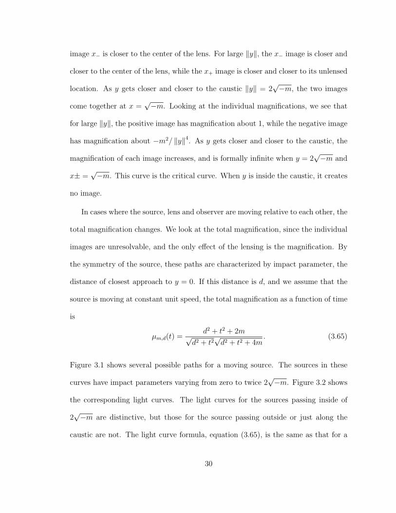
image x− is closer to the center of the lens. For large ‖y‖, the x− image is closer and
closer to the center of the lens, while the x+ image is closer and closer to its unlensed
location. As y gets closer and closer to the caustic ‖y‖ = 2√−m, the two images
come together at x =√−m. Looking at the individual magnifications, we see that
for large ‖y‖, the positive image has magnification about 1, while the negative image
has magnification about −m2/ ‖y‖4. As y gets closer and closer to the caustic, the
magnification of each image increases, and is formally infinite when y = 2√−m and
x± =√−m. This curve is the critical curve. When y is inside the caustic, it creates
no image.
In cases where the source, lens and observer are moving relative to each other, the
total magnification changes. We look at the total magnification, since the individual
images are unresolvable, and the only effect of the lensing is the magnification. By
the symmetry of the source, these paths are characterized by impact parameter, the
distance of closest approach to y = 0. If this distance is d, and we assume that the
source is moving at constant unit speed, the total magnification as a function of time
is
µm,d(t) =d2 + t2 + 2m√
d2 + t2√d2 + t2 + 4m
. (3.65)
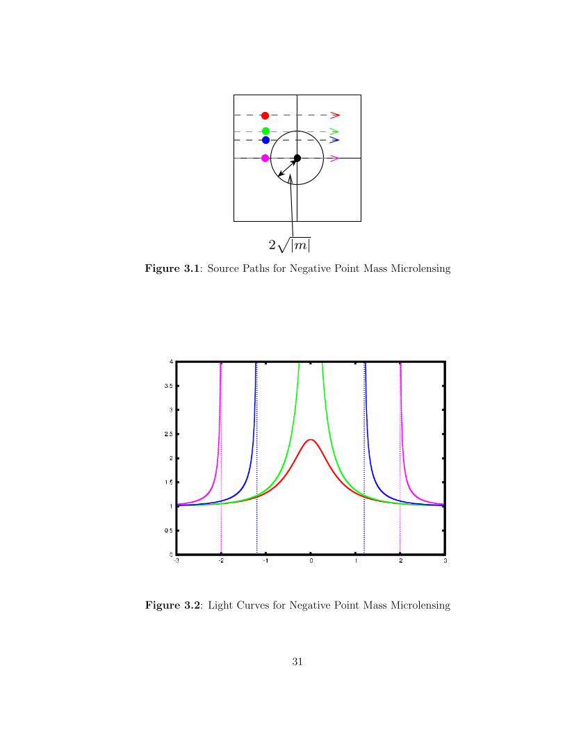
Figure 3.1 shows several possible paths for a moving source. The sources in these
curves have impact parameters varying from zero to twice 2√−m. Figure 3.2 shows
the corresponding light curves. The light curves for the sources passing inside of
2√−m are distinctive, but those for the source passing outside or just along the
caustic are not. The light curve formula, equation (3.65), is the same as that for a
30
2
p
|m|
Figure 3.1: Source Paths for Negative Point Mass Microlensing
Figure 3.2: Light Curves for Negative Point Mass Microlensing
31
positive point mass. Thus if we define
m = −m d =√d2 + 4m, (3.66)
then the light curve for a source passing within d of the line of sight of a mass of m
is the same as that for a source passing within d of the line of sight of a mass of m
µem, ed(t) =d2 + t2 + 2m√
d2 + t2√d2 + t2 + 4m
(3.67)
=d2 + 4m+ t2 − 2m√
d2 + 4m+ t2√d2 + 4m+ t2 − 4m
(3.68)
= µm,d(t). (3.69)
Furthermore, we will see that if we introduce continuous matter we can reproduce
the entire lensing map with a positive mass singularity.
3.6 Complex Formulation
Before incorporating additional features into our lens, it is helpful to reframe the
structure of the lensing map as a map C → C, rather than a map R2 → R2. First
we will consider x as a complex number x1 + ix2, and likewise y and η. The lens
equation becomes
η = η1 + iη2 =
(x1 −
∂ψ
∂x1
)+ i
(x2 −
∂ψ
∂x2
)(3.70)
Taking complex derivatives of η we get
∂η
∂z=
1
2
(∂η
∂x1
− i∂η
∂x2
)=
1
2
(∂η1
∂x1
+ i∂η2
∂x1
− i∂η1
∂x2
+∂η2
∂x2
)=
1
2
(∂η1
∂x1
+∂η2
∂x2
), (3.71)
32
which is real. Here we used the equality of the mixed partials of ψ to cancel the
imaginary terms. Differentiating with respect to z gives
∂η
∂z=
1
2
(∂η
∂x1
+ i∂η
∂x2
)=
1
2
(∂η1
∂x1
− ∂η2
∂x2
+ i
[∂η2
∂x1
+∂η1
∂x2
]). (3.72)
Here no such cancellation occurs. We can also rewrite J = det(dη) as
J =∂η1
∂x1
∂η2
∂x2
− ∂η1
∂x2
∂η2
∂x1
=1
4
∂η1
∂x1
2
+1
2
∂η1
∂x1
∂η2
∂x2
+1
4
∂η2
∂x2
2
−(
1
4
∂η1
∂x1
2
− 1
2
∂η1
∂x1
∂η2
∂x2
+1
4
∂η2
∂x2
2)
−(
1
4
∂η2
∂x1
2
+1
2
∂η2
∂x1
∂η1
∂x2
+1
4
∂η1
∂x2
2)
=
∣∣∣∣∂η∂z∣∣∣∣2 − ∣∣∣∣∂η∂z
∣∣∣∣2 .
(3.73)
Here we extensively used the fact that ∂η2
∂x1= ∂η1
∂x2. Our critical points are located
where J = 0. As we noted above ∂η∂z
is real so the solutions to J = 0 look like
∂η
∂z=
∣∣∣∣∂η∂z∣∣∣∣ eiϕ, (3.74)
for some angle ϕ. Thus our critical curves will be curves parametrized by ϕ.
The caustics will be the images of these critical curves under η. Any points where
the caustics aren’t smooth are characterized by
J(x) = 0 ∇Z(η) = 0. (3.75)
Here Z = − ∂J∂x2
+ i ∂J∂x1
= 2i∂J∂z
, and
∇Z = Z∂
∂z+ Z
∂
∂z. (3.76)
To find the cusps on the caustics we just find the appropriate phase ϕ to solve (3.75).
33
3.7 Lensing by Negative Point Mass Singularities with Con-
tinuous Matter and Shear
Most lensing events on the scale of individual stars take place within a host galaxy.
In these cases, the star itself isn’t the only source of distortion. Two other non-local
factors are also important.
Continuous matter is the first. The presence of evenly dispersed matter in the area
of the lens can produce convergence or divergence. This enters into the dimensionless
potential via a term like
ψcm(x) =κ
2‖x‖2 . (3.77)
This gives us a lensing map of
η(x) = y = (1− κ)x. (3.78)
This is clearly compatible with the complex formulation. The dimensionless mass
density of κ corresponds to a surface mass density of σcπκ.
The other factor is shear from infinity. The presence of a large mass nearby, such
as a nearby galaxy, or an asymmetric distribution such as the disk of the host galaxy,
can introduce a potential of the form
ψsh(x) = −γ2
[(x2
1 − x22
)cos 2θ + 2x1x2 sin 2θ
]. (3.79)
The parameter γ defines the magnitude of the shear, and 2θ determines the preferred
direction of the asymmetric mass distribution or the direction to the large mass. By
the symmetry of our lens, we can assume that θ = 0. This gives us a lensing map of
y =
[1 + γ 0
0 1− γ
]x. (3.80)
34
In complex form this is
y = z + γz. (3.81)
Now we will incorporate all of these features into a single lens. The lensing map
of a negative point mass lens is given by
y = x
(1− m
‖x‖2
). (3.82)
In complex form this is
y = z − m
z. (3.83)
Adding these potentials to that of our singularity gives us the combined lens equation
η(x) =
[1− κ+ γ 0
0 1− κ− γ
]x− m
‖x‖2x, (3.84)
or
η = (1− κ)z + γz − m
z. (3.85)
Our Jacobian is
J =(γ +
m
z2
)2
− (1− κ)2 . (3.86)
So to look for critical points we use equation (3.74) with our η to give us
γ +m
z2 = |1− κ| eiϕ. (3.87)
If κ = 1, then we are looking for points that solve
m
z2 = γ. (3.88)
Which are just two points along the x axis. So we can assume that κ 6= 1. It
simplifies calculation to remove κ from the calculation by defining
γ∗ =γ
|1− κ|m∗ =
m
|1− κ|εκ = sgn(1− κ). (3.89)
35
With those substitutions we now solve
γ∗ +m∗
z2 = eiϕ. (3.90)
This has solutions
z±(ϕ) = ±√
m∗
e−iϕ − γ∗. (3.91)
At this point the only effect that the negative sign on m has had is to rotate our
critical curves by π/2.
z±(ϕ) = ±i
√|m∗|
e−iϕ − γ∗. (3.92)
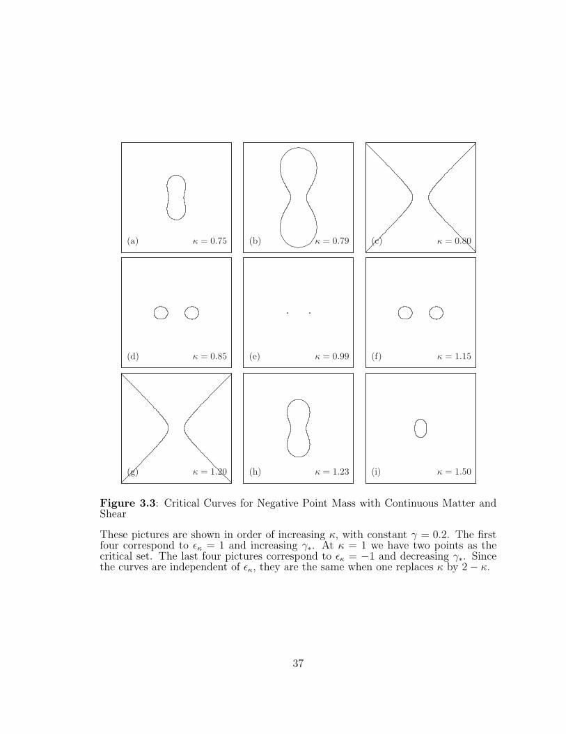
Note that these curves are independent of εκ. For γ∗ 1, the critical curve is given
by an oval with long axis in the x2 direction. As γ∗ grows to 1, the critical curve
develops a waist. For γ∗ > 1, we have two critical curves, small loops on the x1
axis. As γ∗ grows they shrink to the two points for κ = 1. For γ∗ very close to
1, both varieties of critical curves grow to infinity. When γ∗ = 1 our critical curves
degenerate into two curves asymptotic to the lines x2 = ±x1. As γ∗ passes 1, the ends
of the curve open up, pass through infinity, and reseal re-paired. See Figure 3.3 for
the shapes of the critical curves for various values of shear and convergence. These
curves are the same as in the positive mass case, rotated a quarter turn.
To find the cusps we plug our lensing map into (3.75). In our case we have
Z = −4i(γ +
m
z2
) mz3 (3.93)
and equation (3.75) is
0 = (1− κ)Z +(γ +
m
z2
)Z. (3.94)
36
(a) κ = 0.75 (b) κ = 0.79 (c) κ = 0.80
(d) κ = 0.85 (e) κ = 0.99 (f) κ = 1.15
(g) κ = 1.20 (h) κ = 1.23 (i) κ = 1.50
Figure 3.3: Critical Curves for Negative Point Mass with Continuous Matter andShear
These pictures are shown in order of increasing κ, with constant γ = 0.2. The firstfour correspond to εκ = 1 and increasing γ∗. At κ = 1 we have two points as thecritical set. The last four pictures correspond to εκ = −1 and decreasing γ∗. Sincethe curves are independent of εκ, they are the same when one replaces κ by 2− κ.
37
εκ = 1 εκ = −1Shear ϕi Ncusps ϕi Ncusps
0 ≤ γ2∗ < 3/4 ∅ 0 ϕ1, ϕ2 4
3/4 ≤ γ2∗ < 1 ϕ3, ϕ4, ϕ5, ϕ6 8 ϕ1, ϕ2 4
1 < γ2∗ ϕ1, ϕ4, ϕ6 6 ϕ2, ϕ3, ϕ5 6
Table 3.1: Numbers of cusps on caustics for various shear and continuous mattervalues.
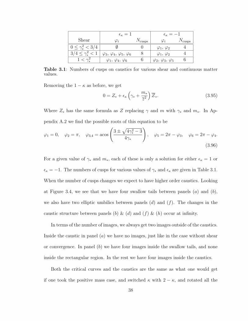
Removing the 1− κ as before, we get
0 = Z∗ + εκ
(γ∗ +
m∗
z2
)Z∗. (3.95)
Where Z∗ has the same formula as Z replacing γ and m with γ∗ and m∗. In Ap-
pendix A.2 we find the possible roots of this equation to be
ϕ1 = 0, ϕ2 = π, ϕ3,4 = acos
(3±
√4γ2
∗ − 3
4γ∗
), ϕ5 = 2π − ϕ3, ϕ6 = 2π − ϕ4.
(3.96)
For a given value of γ∗ and m∗, each of these is only a solution for either εκ = 1 or
εκ = −1. The numbers of cusps for various values of γ∗ and εκ are given in Table 3.1.
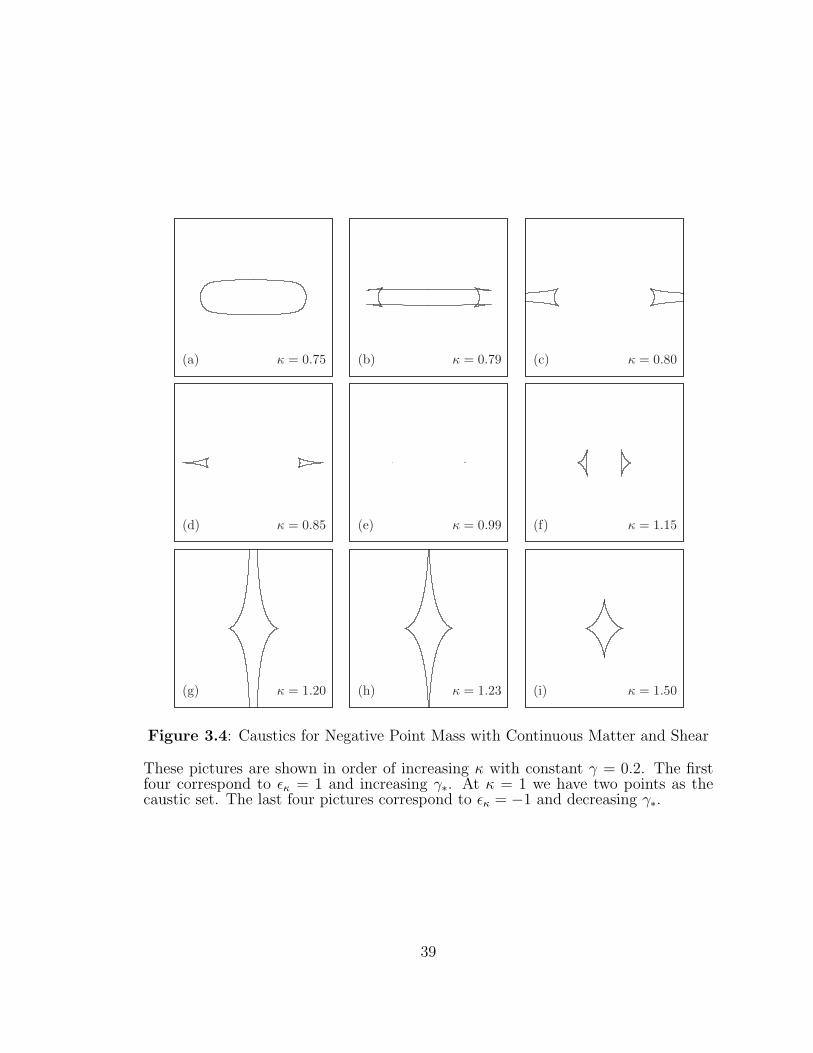
When the number of cusps changes we expect to have higher order caustics. Looking
at Figure 3.4, we see that we have four swallow tails between panels (a) and (b),
we also have two elliptic umbilics between panels (d) and (f). The changes in the
caustic structure between panels (b) & (d) and (f) & (h) occur at infinity.
In terms of the number of images, we always get two images outside of the caustics.
Inside the caustic in panel (a) we have no images, just like in the case without shear
or convergence. In panel (b) we have four images inside the swallow tails, and none
inside the rectangular region. In the rest we have four images inside the caustics.
Both the critical curves and the caustics are the same as what one would get
if one took the positive mass case, and switched κ with 2 − κ, and rotated all the
38
(a) κ = 0.75 (b) κ = 0.79 (c) κ = 0.80
(d) κ = 0.85 (e) κ = 0.99 (f) κ = 1.15
(g) κ = 1.20 (h) κ = 1.23 (i) κ = 1.50
Figure 3.4: Caustics for Negative Point Mass with Continuous Matter and Shear
These pictures are shown in order of increasing κ with constant γ = 0.2. The firstfour correspond to εκ = 1 and increasing γ∗. At κ = 1 we have two points as thecaustic set. The last four pictures correspond to εκ = −1 and decreasing γ∗.
39

images by a quarter turn.
40
Chapter 4
Inverse Mean Curvature Flow
This chapter lays out what we need of the weak inverse mean curvature flow as de-
veloped in [7]. We will follow their exposition closely, omitting many of the technical
details.
4.1 Classical Formulation
Let N be a the smooth boundary of a region in the smooth Riemannian manifold
M . A classical solution of the inverse mean curvature flow is a smooth family x :
N × [0, T ] →M of hypersufaces Nt = x(N, t) satisfying the evolution equation
∂x
∂t=
ν
H. (4.1)
Here ν is the outward pointing normal to Nt and H is the mean curvature of N ,
which must be positive. We use this flow to explore the geometry near a singularity.
For instance we will use the fact that under this flow the Hawking mass is non-
decreasing. This result can be readily shown if we assume that the flow doesn’t have
any discontinuities or singularities. However, easy counterexamples illustrate that
41
this is overly optimistic. The simplest counterexample is given by a thin torus in
R3. Such a torus has positive mean curvature approximately that of a cylinder of
the small radius. The inverse mean curvature flow will tend to increase the small
radius of this torus. However, if it continued without singularities or jumps, the hole
in the torus would eventually shrink to the point where the area of the torus inside
the hole has zero mean curvature and hence the flow couldn’t be continued. Thus
the classical flow is insufficient for our needs.
To remedy this problem, we will follow [7] and recast the flow first in a level
set formulation and then we will move to a weak solution. This will allow the flow
to jump to avoid situations where the curvature of the surface would drop to zero.
In the previous example, the flow would close the interior of the torus as soon as
it is favorable in terms of a certain energy functional. Even with these jumps the
Hawking mass of our surface is still non-decreasing.
4.2 Weak Formulation
First we establish some notation. Let (M, g) be the ambient manifold. Let h be the
induced metric on N . Let Aij = 〈∇eiν, ej〉 be the second fundamental form of N .
Then H is the trace of A with h, and ~H = −νH is the mean curvature vector. Let
E be the open region bounded by N .
The first step toward the weak formulation is a level set formulation. We assume
that the flow is given by the level sets of a function u : M → R. This u is related to
our previous data by
Et := x | u(x) < t , Nt := ∂Et. (4.2)
42
We will also need the following sets
E+t := int x | u(x) ≥ t , N+
t := ∂E+t (4.3)
Where ∇u 6= 0, Et = E+t and Nt = N+
t .
Anywhere that u is smooth and ∇u 6= 0, then we have a foliation by smooth
surfaces Nt, with normal vector ν = ∇u/ |∇u|. The mean curvature of these surfaces
is given by divN(ν) and the flow velocity is given by 1/ |∇u|, so equation (4.1)
becomes
divM
(∇u|∇u|
)= |∇u| . (4.4)
This equation is degenerate elliptic. To remedy this we introduce the functional
JKu (v):
Ju(v) = JKu (v) =
∫K
|∇v|+ v |∇u| . (4.5)
Where K is a compact set in M . If we take the Euler-Lagrange equation of this
functional, and replace v with u, we get back equation (4.4). For each u we get a
different Ju. Hence what we want is a function u which minimizes its own Ju.
Definition 4.2.1. Let u be a locally Lipschitz function on the open set Ω in M .
Then u is a weak (sub-, super-) solution of equation (4.4) on Ω exactly when
JKu (u) ≤ JK
u (v) (4.6)
for all locally Lipschitz functions v (≤ u,≥ u) which only differ from u inside a
compact set K contained in Ω.
It is worth noting that Ju(min(v, w)) + Ju(max(v, w)) = Ju(v) + Ju(w). To see
this, construct Kv = x ∈ K | v(x) < w(x), and divide the integrals on the left into
43
integrals over Kv and K \ Kv. Then regroup then and recombine to get the right
hand side. This tells us that if u is a both a weak supersolution and subsolution,
then it is a weak solution.
We will also need a related functional of the level sets.
Definition 4.2.2. If F is a set of locally finite perimeter, and ∂∗F is its reduced
boundary, then we define
Ju(F ) = JKu (F ) = |∂∗F ∩K| −
∫F∩K
|∇u| . (4.7)
For any locally Lipschitz function u and compact K contained in A. We say that E
minimizes Ju in A (on the inside, outside) if
JKu (E) ≤ Ju(F ) (4.8)
for all F that differs from E in some compact K in A (with E ⊆ F , E ⊇ F .) A
similar argument tells us that if E minimizes Ju exactly when it minimizes Ju on the
inside and outside.
These two formulations are equivalent.
Lemma 4.2.3. Let u be a locally Lipschitz function in the open set Ω. Then u is a
weak (sub-, super-) solution of equation (4.4) exactly when for each t, Et = u < t
minimizes Ju in Ω (on the inside, outside).
Proof. Lemma 1.1 in [7].
We now define the initial value problem. Let E0 be an open set with C1 boundary.
We say that u ∈ C0,1loc and the associated Et for t > 0 is a weak solution of (4.4) with
44
initial condition E0 if either
E0 = u < 0 and u minimizes Ju on M \ E0
or
Et = u < t minimizes Ju in M \ E0 for t > 0.
(4.9)
These two conditions are equivalent by Lemma 1.2 in [7]. Showing the regularity
of Nt and N+t is nontrivial, but we won’t reproduce it here.
Theorem 4.2.4. Let n < 8. Let U be an open set in a domain Ω. Let f be a bounded
measurable function on Ω. Consider the functional
|∂F |+∫
F
f (4.10)
on sets containing U and compactly contained in Ω. Suppose E minimizes this func-
tional.
1. If ∂U is C1, then ∂E is a C1 submanifold of Ω.
2. If ∂U is C1,α, 0 < α ≤ 1/2, then ∂E is a C1,α submanifold of Ω. The C1,α
estimates depend only on the distance to ∂Ω, ess sup |f |, C1,α bound for ∂U ,
and C1 bounds on the metric in Ω.
3. If ∂U is C2 and f = 0, then ∂E is C1,1, and C∞ where it doesn’t touch U .
Our initial value formulation falls into this category of problem. So our Nt’s and
N+t ’s are C1,α. Furthermore
lims→t−
Ns = Nt lims→t+
Ns = N+t (4.11)
in local C1,β convergence 0 < β ≤ α.
The locations where Nt 6= N+t correspond to the jumps discussed earlier. To
examine these areas we need to introduce minimizing hulls.
45
Definition 4.2.5. Let Ω be an open set. We call E a minimizing hull if
|∂∗E ∩K| ≤ |∂∗F ∩K| (4.12)
for any F containing E with F \ E in K a compact set in Ω. We say E strictly
minimizes if equality implies that E and F agree in Ω up to measure zero.
The intersection of (strictly) minimizing hulls is a (strictly) minimizing hull. So,
given a set E we can intersect all of the strictly minimizing hulls which contain
E. This gives, up to measure zero, a unique set E ′ that we will call the strictly
minimizing hull of E. Since E ′ is strictly minimizing, E ′′ = E ′.
Solutions to the initial value problem given by equation (4.9), have level sets that
are minimizing hulls as follows.
Lemma 4.2.6. Suppose that u is a solution to (4.9). Assume that M has no compact
components. Then:
• For t > 0, Et is a minimizing hull in M .
• For t > 0, E+t is a strictly minimizing hull in M .
• For t > 0, E ′t = E+
t if E+t is precompact.
• For t > 0, |∂Et| =∣∣∂E+
t
∣∣, provided that E+t is precompact.
• Exactly when E0 is a minimizing hull |∂E0| =∣∣∂E+
0
∣∣This is “Minimizing Hull Property (1.4)” in [7]. These minimizing properties
characterize how the weak flow differs from the classical flow. The classical flow
runs into trouble when the mean curvature changes sign. If the mean curvature is
46
negative on a part of Nt, we could decrease the area of Nt be flowing that patch out.
So the weak flow avoids these areas by making sure that N+t is always the outermost
surface with its area. This sometimes necessitates jumping.
The existence and uniqueness of solutions to equation (4.4) with initial data are
beyond our scope. However, for completeness, here is the existence and uniqueness
theorem (3.1) from [7].
Theorem 4.2.7. Let M be a complete, connected Riemannian n-manifold without
boundary. Suppose there exists a proper, locally Lipschitz, weak subsolution of (4.9)
with a precompact initial condition.
Then for any nonempty, precompact, smooth open set E0 in M , there exists a
proper, locally Lipschitz solution u of (4.9) with initial condition E0, which is unique
in M \ E0. Furthermore, the gradient of u satisfies the estimate
|∇u(x)| ≤ sup∂E0∩Br(x)
H+ +C(n)
r, a.e. x ∈M \ E0, (4.13)
for each 0 < r ≤ σ(x).
The function σ(x) depends on the Ricci curvature of M near E0, but is always
positive. More importantly, the requirement for a subsolution is satisfied by any
asymptotically flat manifold. A function like ln(R) in the asymptotic end will suffice.
4.3 Useful Properties of Weak IMCF
Now that we have outlined the flow, we will describe some useful properties.
Lemma 4.3.1. Let (Et)t>0 solve (4.9) with initial condition E0. As long as Et
remains precompact, we have the following:
47
• e−t |∂Et| is constant for t > 0.
• If E0 is its own minimizing hull then |∂Et| = et |∂E0|.
Proof. Since each Et minimizes the same functional, they must all have the same
value for Ju(Et). Applying the co-area formula to the integral in Ju gives
Ju(Et) = |∂Et| −∫ t
0
1
|∇u|
∫∂Es
|∇u| dAds (4.14)
= |∂Et| −∫ t
0
|∂Es| ds. (4.15)
Which has solutions of the form Cet. By the minimizing hull properties, we could
replace ∂Et with ∂E+t for t > 0. Since ∂E+
0 is the limit of ∂Es as s 0, C =∣∣∂E+
0
∣∣.If E0 is its own minimizing hull then |∂E0| =
∣∣∂E+0
∣∣, and C = |∂E0|.
The next two lemmas tell us that when the classical solution exists, it agrees with
the weak solution.
Lemma 4.3.2. Let (Nt)c≤t<d be a smooth family of surfaces of positive mean curva-
ture that solve (4.1) classically. Let u = t on Nt, u < c inside Nc, and Et = u < t.
Then for c ≤ t < d, Et minimizes Ju in Ed \ Ec.
Lemma 4.3.3. Let E0 be a precompact open set in M such that ∂E0 is smooth with
H > 0 and E0 = E ′0. Then any unique solution (Et)0<t<∞ of (4.9) with initial
condition E0 coincides with the unique smooth classical solution for a short time,
provided Et remains precompact for a short time.
The authors of [7] point out that the stopping point for these theorems will be
when either Et is no longer a minimizing hull, the mean curvature goes to zero, or
the second fundamental form is unbounded.
48
The proof of existence and uniqueness of the weak flow are beyond the scope of
this thesis. However, the method is as follows. First they assume the existence of a
subsolution v. Then they solve the regularized problem
Eεuε := div
∇uε√|∇uε|2 + ε2
−√|∇uε|2 + ε2 = 0 in ΩL
uε = 0 on ∂E0
uε = L− 2 on ∂FL.
(4.16)
Where FL = v < L, ε is small, and L is large, but bounded in size by a function
of ε. Then they take the limit as L → ∞, ε → 0. Some estimates on |∇u| and H
guarantee that the solution passes to the limit.
The authors also proved that in the asymptotic regime, the Hawking mass of the
level sets of the flow converges to the ADM mass of the manifold
Theorem 4.3.4. Assume that M is asymptotically flat and let (Et)t≥t0 be a family
of precompact sets weakly solving (4.1) in M . Then
limt→∞
mH(Nt) ≤ mADM(M). (4.17)
Proof. They show that Nt must approach coordinate spheres in the asymptotic
regime. This is their Lemma 7.4.
4.4 Geroch Monotonicity
The Geroch Monotonicity formula says that the Hawking mass is nondecreasing
under the inverse mean curvature flow. The original use of this was to propagate the
mass of a surface out to infinity to compare to the ADM mass using IMCF. However,
49
it also provides bounds on integrals of H and area near the surface. We will first
show how it arises in the smooth case, and then extend it over the jumps in the weak
flow.
In the smooth case, we simply recall that the Hawking mass is given by
mH =
√|N |16π
(1− 1
16π
∫N
H2
). (4.18)
The first variation of area is given by
d
dtdA = Hη dA. (4.19)
Thus under smooth IMCF we have ddtdA = dA. The variation of H is given by
dH
dt= ∆(−η)− |A|2 η − Rc(ν, ν)η. (4.20)
Thus if we look at the integral∫H2 dA under IMCF we get
d
dt
∫H2 dA =
∫H2 − 2
|∇NH|2
H2+ 2 |A|2 − 2 Rc(ν, ν) dA. (4.21)
The Gauss equation contracts to give
K = K12 + λ1λ2 =R
2− Rc(ν, ν) +
1
2(H2 −
∣∣A2∣∣) (4.22)
Here K and R are the scalar curvatures of N and M respectively, K12 is the sectional
curvature of M in the plane tangent to N , and λi are the principal curvatures of N .
Using this equation to cancel the Rc term gives us the following equation
d
dt
∫N
H2 =
∫N
2K − 2|∇NH|2
H2− |A|2 −R (4.23)
=
∫N
4K −R− 2|∇NH|2
H2− 1
2(λ1 + λ2)
2 − 1
2(λ1 − λ2)
2 . (4.24)
50
If R > 0,
d
dt
∫N
H2 = 4πχ(Nt)−1
2
∫N
H2 −∫
N
2|∇NH|2
H2+
1
2(λ1 − λ2)
2 . (4.25)
If Nt is connected,
d
dt
∫N
H2 ≤ 8π
(1− 1
16π
∫N
H2
). (4.26)
In addition recall that |Nt| = |N0| et in the smooth case. Thus we get that
√16π
d
dtmH =
d
dt
[et/2
(1− 1
16π
∫N
H2
)](4.27)
≥[1
2et/2
(1− 1
16π
∫N
H2
)− et/2 8π
16π
(1− 1
16π
∫N
H2
)]= 0. (4.28)
Hence the Hawking mass is nondecreasing.
To cover the gap, we simply note that at the jumps, the new surface E ′t = E+
t is
a minimizing hull for Et. That means that where their boundaries differ, ∂E ′t must
have zero mean curvature (else a variation could decrease its area keeping it outside
of Et, contradicting its minimizing property.) Hence∫∂Et
H2 ≥∫
∂E′t
H2. (4.29)
Thus since |∂E ′t| = |∂Et| for t > 0, we see that the, even at jumps, the Hawking
mass can’t decrease. This doesn’t cover the possibility of dense jumping, or similar
pathological behavior, but extending the Geroch formula to those cases requires using
the elliptic regularization.
The statement of Geroch Monotonicity given in [7] for one boundary component
is as follows
51
Theorem 4.4.1. Let M be a complete 3-manifold, E0 a precompact open set with
C1 boundary satisfying∫
∂E0|A|2 < ∞, and (Et)t>0 a solution to (4.9) with initial
condition E0. If E0 is a minimizing hull then
mH(Ns) ≥ mH(Nr)+
+1
(16π)3/2
∫ s
r
[16π − 8πχ(Nt) +
∫Nt
(2 |D logH|2 + (λ1 − λ2)
2 +R)]dt (4.30)
for 0 ≤ r ≤ s provided Es is precompact.
52
Chapter 5
Negative Point Mass Singularity Results
5.1 Negative Point Mass Singularities and IMCF
Although we do not need this fact, it is interesting to note that near a negative point
mass singularity, we can define the inverse mean curvature flow. Even though there
is no initial surface to start from we can take a limit of solutions to IMCF for starting
surfaces that converge to p. This actually defines a unique solution u to the weak
inverse mean curvature flow. This was shown in recent work by Jeffrey Streets [10].
Theorem 5.1.1 ([10]). Let M3 be an asymptotically flat manifold with finitely many
singularities at pi. Then there is a unique solution to (4.4) on M \ pi.
In this case since the area of the level sets is exponential in time, and surfaces
near the singularities have vanishing area. Thus this flow only reaches the singularity
at time −∞.
Streets also showed that these surfaces were the best possible surfaces, in terms
of the Hawking mass, as in the following theorem.
53
Theorem 5.1.2 ([10]). Let St be the family of hypersurfaces defining the solution to
IMCF above. Let Pt be any other family of hypersurfaces approaching the singularity.
Then,
limt→−∞
mH(Pt) ≤ limt→−∞
mH(St). (5.1)
We can also extend Geroch Monotonicity down to t = 0 in the case where our
initial surface has negative Hawking mass.
Lemma 5.1.3. Let Σ be a surface in an asymptotically flat 3 manifold. Let Σ′ be
the boundary of the minimizing hull of Σ. Let Σ or Σ′ have negative Hawking mass.
Then
mH(Σ) ≤ mH(Σ′). (5.2)
Proof. If Σ′ has nonnegative Hawking mass then mH(Σ′) ≥ 0 ≥ mH(Σ) and we are
done. Thus we can assume that Σ′ has negative Hawking mass. Since Σ′ has negative
Hawking mass, it must intersect Σ on a set of positive measure. Otherwise, Σ′ would
be a minimal surface, with Hawking mass√
|Σ′|16π
> 0. We define the following sets:
Σ0 = Σ′ ∩ Σ Σ+ = Σ′ \ Σ0 Σ− = Σ \ Σ0 (5.3)
Recalling that |Σ+| ≤ |Σ−| by the minimization property, and that H = 0 on Σ+,
we observe the following:
0 > mH(Σ′) =
√|Σ0|+ |Σ+|(16π)3/2
(16π −
∫Σ0
H2
)(5.4)
≥√|Σ0|+ |Σ−|(16π)3/2
(16π −
∫Σ0
H2
)(5.5)
≥√|Σ0|+ |Σ−|(16π)3/2
(16π −
∫Σ0
H2 −∫
Σ−
H2
)= mH(Σ). (5.6)
54
With this lemma and Geroch Monotonicity we can prove the following lemma.
Lemma 5.1.4. Let (M, g) be an asymptotically flat manifold with ADM mass m,
nonnegative scalar curvature and a single regular negative point mass singularity
p. Let Σi be a smooth family of surfaces converging to p, which eventually have
negative Hawking mass. Then for sufficiently large i,
mH(Σi) ≤ m. (5.7)
Proof. Since for large enough i, Σi has non-positive Hawking mass, we can apply
Lemma 5.1.3 to show that Σ′i must have larger Hawking mass. From this surface, we
start Inverse Mean Curvature Flow. Theorem 4.4.1 tells us that the Hawking mass
of the surfaces Nt defined by IMCF starting with Σ′i only increase. Theorem 4.3.4
tells us that the increasing limit of the Hawking masses these surfaces is less than
the ADM mass. Thus the Hawking mass of the starting surface was also less than
the ADM mass.
Now we relate the limit of the Hawking masses to the regular mass.
Lemma 5.1.5. Let (M, g) be an asymptotically flat manifold with nonnegative scalar
curvature and a single regular negative point mass singularity p. Then there is a
smooth family of surfaces Σi converging to p such that
limi→∞
mH(Σi) = −1
4
(1
π
∫Σ
ν(ϕ)4/3 dA
)3/2
= mR(p). (5.8)
Proof. The Hawking mass of a surface Σi is given by
mH(Σi) =
√|Σi|16π
(1− 1
16π
∫Σi
H2 dA
). (5.9)
55
Since the areas of the surfaces are converging to zero we have
limi→∞
mH(Σi) = − limi→∞
√|Σi|
(16π)3/2
∫Σi
H2 dA. (5.10)
By the Holder inequality this is bounded as follows
−√|Σi|
(16π)3/2
∫Σi
H2 dA ≤ − 1
(16π)3/2
(∫Σi
H4/3 dA
)3/2
. (5.11)
Switching to the resolution space, we use the formula
H = ϕ−2H + 4ϕ−3ν(ϕ). (5.12)
Putting this into the previous equation we get∫Σi
H4/3 dA =
∫Σi
(ϕ−2H + 4ϕ−3ν(ϕ)
)4/3ϕ4 dA (5.13)
=
∫Σi
(ϕH + 4ν(ϕ)
)4/3dA. (5.14)
Since ϕ is zero on Σ and H is bounded, the first term goes to zero. The second term
converges since the family of surfaces Σi are converging smoothly.
limi→∞
∫Σi
(ϕH + 4ν(ϕ)
)4/3dA = 44/3
∫Σ
ν(ϕ)4/3 dA. (5.15)
Combining all of these equations we have
limi→∞
mH(Σi) ≤ −1
4
(1
π
∫Σ
ν(ϕ)4/3 dA
)3/2
= mR(p). (5.16)
To see when this estimate is sharp, we look at inequality (5.11) since that is the only
inequality is our estimate. In the limit, this inequality is an equality exactly when
the ratio of the maximum and minimum values of H approaches 1. We choose a
56
resolution such that ν(ϕ) = 1 on the boundary. We also choose a family of surfaces
Σi given by level sets of ϕ. Then if we look at the ratio
limϕ→0
Hmin
Hmax
= limϕ→0
ϕHmin + 4ν(ϕ)
ϕHmax + 4ν(ϕ), (5.17)
and remember that H is bounded, we see that the ν(ϕ) terms dominate, and as
ϕ→ 0, this ratio approaches 1. Thus with this resolution and this family of surfaces,
inequality (5.16) will turn to an equality.
With these results we can prove the following theorem
Theorem 5.1.6. Let (M, g) be an asymptotically flat manifold with nonnegative
scalar curvature and a single regular negative point mass singularity p. Then the
ADM mass of M is at least the mass of p.
Proof. First consider the case when p can be enclosed by a surface, Σ, with nonneg-
ative Hawking mass. The minimizing hull of a surface with nonnegative Hawking
mass has nonnegative Hawking mass. Thus we can run IMCF from Σ′, and the
AMD mass of M is at least mH(Σ′) ≥ 0. However, the regular mass of p is always
nonpositive so in this case we are done.
Now assume that p cannot be enclosed by a surface with nonnegative Hawking
mass. By Lemma 5.1.4 we know that the ADM mass is greater than the Hawking
masses of any sequence of surface converging to p which have negative Hawking
mass. By Lemma 5.1.5 we know that there is a family of surfaces converging to p
which have the mass of p as the limit of their Hawking mass, hence the ADM mass
is greater then their Hawking masses which limit to the regular mass.
57
This can be extended to general negative point mass singularities. However, first
we need to consider the effect of multiplication by a harmonic conformal factor on
the ADM mass of a manifold.
Lemma 5.1.7. Let (M3, g) be an asymptotically flat manifold. Let ϕ be a harmonic
function with respect to g with asymptotic expansion
ϕ = 1 +C
|x|g+O
(1
|x|2g
). (5.18)
Then, if the ADM mass of (M3, g) is m, the ADM mass of (M3, ϕ4g) is m+ 2C.
Proof. This is a direct calculation. We write gϕ = gϕ4, and calculate, only keeping
the terms of lowest order in 1/ |x| since we are taking limits as |x| → ∞.
mϕ = lim|x|→∞
1
16π
∫Sδ
(gϕ
ij,i − gϕii,j
)nj dA (5.19)
= lim|x|→∞
ϕ4
16π
∫Sδ
(gij,i − gii,j)nj dA+ lim
|x|→∞
ϕ3
4π
∫Sδ
(δijϕi − δiiϕj)nj dA (5.20)
= lim|x|→∞
ϕ4m+ lim|x|→∞
ϕ3 lim|x|→∞
1
4π
∫Sδ
(ϕj − 3ϕj)nj dA (5.21)
= m+ lim|x|→∞
1
2π
∫Sδ
ϕjnj dA (5.22)
= m+ lim|x|→∞
1
2π
∫Sδ
〈∇ϕ, ν〉 dA (5.23)
= m+ 2C. (5.24)
Using this we can now extend Theorem 5.1.6 to a general singularity.
58
Theorem 5.1.8. Let (M, g) be an asymptotically flat manifold with nonnegative
scalar curvature and a single negative point mass singularity p. Then m, the ADM
mass of M , is at least the mass of p.
Proof. If the capacity of p is nonzero, then the statement is trivial. Thus we assume
the capacity of p is zero. Using the terminology of Definition 2.3.4, Theorem 5.1.6
tells us that the ADM mass of (M,h4i g) is at least the mass of the regular singularity
at Σi = pi. Each hi is defined by the equations
∆hi = 0 (5.25)
limx→∞
hi = 1 (5.26)
hi = 0 on Σi. (5.27)
Thus it has asymptotic expansion
hi = 1− Ci
|x|+O
(1
|x|2
). (5.28)
Where Ci is the capacity of Σi. Thus, the ADM mass, mi, of (M,h4i g) is given by
m− 2Ci. Now we know that mi ≥ mR(pi). Taking lim of both sides gives us
limi→∞
mi ≥ limi→∞
mR(pi) (5.29)
Since Ci is going to zero, the left hand side is simply m, and so has no dependence
on which Σi we chose in our mass calculation. Thus we get
m ≥ supΣi
limi→∞
mR(pi). (5.30)
as desired.
59
5.2 Capacity Theorem
Perhaps the most important new results of this thesis are Theorems 5.2.4 and 5.2.5
which relate the capacity of a point to the Hawking masses of surfaces near that
point.
The capacity of a surface provides a measure of its size as seen from infinity. We
extend the definition of the capacity of surface to the capacity of a negative point
mass singularity. We then show that if a NPMS has non-zero capacity the Hawking
mass of any family of surfaces converging to it must go to negative infinity. First the
definition of capacity:
Definition 5.2.1. Let Σ be surface in an asymptotically flat manifold M . Define
the capacity of Σ by
C(Σ) = inf
∫M
‖∇ϕ‖2 dV
∣∣∣∣ϕ(Σ) = 1, ϕ(∞) = 0
. (5.31)
It is worth noting that if Σ and Σ′ are two surfaces in M so that Σ divides M
into two components, one containing infinity and the other containing Σ′, then
C(Σ′) ≤ C(Σ) (5.32)
since the infimum is over a larger set of functions.
We will next define the capacity of a singular point. The natural definition is the
one we want.
Definition 5.2.2. Let p be singular point in an asymptotically flat manifold M .
Chose a sequence of surfaces Σi of decreasing diameter enclosing p. Then define the
capacity of p by the limit of the capacities of Σi.
60
Before using this definition we have to show that it is unique.
Lemma 5.2.3. Let Σi and Σi be two sequences of surfaces approaching the point p.
If limC(Σi) = K, limC(Σi) = K. Hence C(p) is well defined.
Proof. Since the Σi are going to p, for any given Σi0 , we can choose i0 such that for
all i > i0, Σi is contained within Σi0 . Thus if ϕ is a capacity test function for Σi0 ,
i.e. ϕ(Σi0) = 1 and ϕ → 0 at infinity, then ϕ is also a capacity test function for Σi.
Since C(Σi) is taking the infimum over a larger set of test functions than C(Σi0),
C(Σi) ≤ C(Σi0). Thus if we create a new sequence of surfaces Σi, alternately choosing
from Σi and Σi, such that each surface contains the next we get a nonincreasing
sequence of capacities. Thus if either original sequence of surfaces has a limit of
capacity, then this new sequence must as well, and it must be the same. Hence,
limi→∞C(Σi) = limi→∞C(Σi).
Now we look at the relationship between capacity and the Hawking mass of a
surface. We will use techniques similar to those used in [4].
Theorem 5.2.4. Let M be an asymptotically flat 3 manifold with nonnegative scalar
curvature, and negative point mass singularity p. Let Σi be a family of surfaces
converging to p. Assume each Σi is a minimizing hull. Assume the areas of Σi
are going to zero. Then if the Hawking mass of the surfaces is bounded below, the
capacities of surfaces of foliation near p must go to zero.
Proof. To use Geroch monotonicity, we need to know that our IMCF surfaces stay
connected. In the weak formulation of IMCF, the level sets Σt always bound a
region in M . Thus if Σt is not connected, one of its components Σ∗t must not bound
61
a region. That is, Σ∗t is not homotopic to a point in M . Since M is smooth, it
must have finite topology on any bounded set. Thus we know that near p, there is a
minimum size for a surface that does not bound a region. Call this size Amin. Thus
if we have any surface that does not bound a region, it must have area greater then
Amin. According to Lemma 4.3.1 the area of our surfaces grow exponentially. Thus if
we restrict ourselves to starting IMCF with a surface with area Amin/e, and only run
the flow for time 1, we will stay connected. At first glance it seems we may need to
worry about the jumps in weak IMCF, however Geroch monotonicity doesn’t depend
on smoothness of the flow, and neither does the area growth formula. Lemma 4.3.1
holds from t = 0. Thus even with jumps, the area of our surfaces will remain below
Amin.
Now recall that capacity of a surface is defined by
C(Σ) = inf
∫M
‖∇ϕ‖2 dV
∣∣∣∣ϕ(Σ) = 1, ϕ(∞) = 0
. (5.33)
Here, the integral is only over the portion of M outside of Σ. Call this integral, E(ϕ),
the energy of ϕ. Thus for any ϕ with ϕ(∞) = 0 and ϕ(Σ) = 1 we have E(ϕ) ≥ C(Σ).
So we will find an estimate that relates the Hawking mass and the energy of a test
function ϕ.
Choose a starting surface Σ with sufficiently small starting area. Let f be the
level set function of the associated weak IMCF starting with the surface Σ. Call the
resulting level sets Σt. Now if we use a test function of the form ϕ = u(f), then the
energy of ϕ is given by
E(ϕ) =
∫M
‖∇f‖2 (u′)2dV. (5.34)
62
Since f is given by IMCF, we know that ‖∇f‖ = H where H is the mean curvature
of the level sets. Next we will use the co-area formula. This states that if we have
a function z on a domain Ω, and a function h : R → R so that the range of h(z) is
[a, b], then ∫Ω
h dV =
∫ b
a
h(z(t))
∫St
|∇z(t)| dAt dt. (5.35)
Here St are the level sets of h(z(t)). If we use the co-area formula with the foliation
Σt, our integral becomes
E(ϕ) =
∫ ∞
0
(u′(t))2
∫Σt
|H| dAt dt. (5.36)
Here the co-area gradient term cancels one of the ‖∇f‖ terms. Now we will bound
the interior integral of curvature. We know that IMCF causes the Hawking mass to
be nondecreasing in t. We first rewrite the definition of the Hawking mass mH(Σit) =
m(t) as: ∫H2dAt = 16π
(1−m(t)
√16π
A(t)
). (5.37)
Here A(t) is the area of Σt. Since the Hawking mass is nondecreasing under IMCF
we have: ∫H2dAt ≤ 16π
(1−m(0)
√16π
A(t)
). (5.38)
Thus we can use Cauchy-Schwartz to get:
∫|H| dAt ≤
√A(t)
√√√√16π
(1−m(0)
√16π
A(t)
). (5.39)
63
We can rewrite this as: ∫|H| dAt ≤
√αA(t) + β
√A(t). (5.40)
Furthermore, since A(t) grows exponentially in t, we can write this as:∫|H| dAt ≤
√αet + βet/2 = v(t). (5.41)
Where A0 has been absorbed into α and β. Thus our energy formula has become
E(ϕ) ≤∫ ∞
0
(u′(t))2v(t) dt. (5.42)
with
v(t) =√αet + βet/2 (5.43)
where α = 16πA0, β = (16π)3/2A1/20 |m0|, and A0 is A(Σ0). This means we can pick
our test function u(t) to be as simple as:
u(t) =
1− t 0 ≤ t ≤ 1
0 t ≥ 1(5.44)
Then our integral becomes:
E(ϕ) ≤∫ 1
0
v(t)dt
=
∫ 1
0
√αet + βet/2 dt
=
∫ 1
0
et/4√αet/2 + β dt
= 4
∫ e1/4
1
√αx2 + β dx
≤ 4
∫ e1/4
1
√αx+
√β
= 2√α(e1/2 − 1) + 4
√β(e1/4 − 1)
≤ 2√α+ 2
√β.
64
Since mH(Σ) ≤√
|Σ|16π
, m0 is bounded above. By assumption m0 is bounded below,
so α and β are bounded by multiples of A0 and√A0 respectively. Thus E(ϕ) goes to
zero if A0 → 0 and m0 is bounded. Hence C(p) must be zero since it is the infimum
over a positive set with elements approaching zero.
Theorem 5.2.5 (Capacity Theorem). Let M be an asymptotically flat 3 manifold
with nonnegative scalar curvature, and negative point mass singularity p, such that
there exists a family of surfaces, Σi, converging to p with area going to zero. Then if
the capacity of p is nonzero, the Hawking masses of the surfaces Σi must go to −∞.
Proof. Any such family of surfaces will generate a family Σ′i of minimizing hulls that
will also converge to p. By Lemma 5.2.4, the masses of Σ′i must go to −∞. Thus
the masses of Σ′i must go to −∞. Thus for sufficiently large i, the masses of the
minimizing hulls are all negative. From then on Lemma 5.1.3 applies, and the masses
of Σi must be less then the masses of Σ′i. Hence they also converge to −∞.
65
Chapter 6
Symmetric Singularities
In this chapter we will look at some more examples of negative point mass singu-
larities. The symmetry ansatz provides more structure than in the definition of a
NPMS.
6.1 Spherical Solutions
A spherically symmetric manifold, M , has a metric given by
ds2 = dr2 +A(r)
4πdS2. (6.1)
We can directly calculate that the scalar curvature of M is given by
R =16πA+ A′2 − 4AA′′
2A2. (6.2)
For this manifold to be asymptotically flat it is necessary for the Hawking masses of
the coordinate spheres to approach a constant. The Hawking mass of a coordinate
sphere is given by
mH(S) =
√A
16π
(1− 1
16π
A′2
A
). (6.3)
66
Due to the spherical symmetry of the manifold, we know that if IMCF is started
with coordinate spheres, it must continue with coordinate spheres. Thus we know
that this quantity must be non-decreasing. For this manifold to be asymptotically
flat, this quantity must have a limit at ∞. This limit is the ADM mass.
The only possible location for a singularity in such a manifold is at the origin.
We can find a straight forward function to resolve the singularity. We need a smooth
function ϕ such that
limr→∞
A(r)
ϕ4= 4π, (6.4)
or any other constant.
Multiplying by ϕ−4 to find the model space changes our metric to the form
ds2 = dρ2 +A(ρ)
4πdS2. (6.5)
Where A goes to 4π as ρ approaches zero. Let Σ be the surface ρ = 0. The behavior
of ϕ away from the singularity is very flexible as long it is bounded, nonzero, and
goes to one at infinity. In order for this to be a regular singularity, we need that ρ
be well defined. Thus we must require
ρ(r) =
∫ r
0
ϕ−2dr =
∫ r
0
dr
A1/2(r)<∞ (6.6)
for finite r. Any spherically symmetric singularity with this condition on A(r) must
be regular. The regular mass is given by
mR = −1
4
(1
π
∫Σ
ν(ϕ)4/3dA
)3/2
. (6.7)
Since we have only defined the asymptotic behavior of ϕ near r = 0, we will compute
everything as limits as r goes to zero. First we need to find ν(ϕ). Since ρ =∫ r
0ϕ−2dr,
67
a chain rule calculation of ∂ϕ∂ρ
yields
ν(ϕ) = ϕ2∂ϕ
∂r. (6.8)
Putting this in and expanding the other terms in the definition of the regular mass
gives us
mR = − limr→0
1
4
(1
π
∫Σr
(ϕ2∂ϕ
∂r
)4/3
ϕ−4dA
).3/2 (6.9)
= − limr→0
1
4
1
π3/2A3/2(r)ϕ−2
(∂ϕ
∂r
)2
(6.10)
Using equation (6.4) and l’Hopital’s rule we find that
∂ϕ
∂r=
1
16πϕ3
∂A
∂r(6.11)
Continuing from above
mR = − limr→0
1
4
1
π3/2
1
256π2ϕ−8A3/2A′2
= − limr→0
1
1024π7/2
16π2
A2A3/2A′2
= − limr→0
1
64π3/2
A′2
A1/2.
(6.12)
This agrees with the limit of the Hawking masses of coordinate spheres as r → 0 and
hence A→ 0 as well.
For completeness, we can also examine the capacity of the central point in these
solutions. The capacity of a coordinate sphere in an asymptotically flat spherically
symmetric manifold is given by the 1/ρ term in of the harmonic function that is 1
on the sphere and 0 at infinity. Since harmonic functions have constant flux with
68
respect to the outward normal, we could also describe this function as the constant
flux function which goes to 0 at infinity and 1 on the coordinate sphere. Then the
capacity of the sphere is given by the flux constant of this function, divided by −4π.
Reversing this definition we define the following function:
Definition 6.1.1. Let (M, g) be an asymptotically flat spherically symmetric man-
ifold. Let f be the radial function that has constant outward flux −4π through
coordinate spheres and goes to zero at infinity. Call f the radial capacity function
for (M, g).
This definition allows the following lemma.
Lemma 6.1.2. Let f(r) be the radial capacity function for the manifold (M, g).
Then the capacity of the coordinate sphere at r = r0 is given by f(r0)−1.
Proof. Consider the function f(r)/f(r0). This function is 1 on the coordinate sphere
r = r0, goes to zero at infinity, and is harmonic. In the asymptotic regime its 1/ρ
coefficient is 1/f(r0). Thus this is the capacity of the sphere r = r0.
Thus the capacity of the central point is given by limr→0 f(r)−1. To calculate this
value we first note that
df
dr= − 4π
A(r)(6.13)
since f has constant flux −4π. Thus
f(r) = −∫ ∞
r
f ′(r)dr = 4π
∫ ∞
r
dr
A(r). (6.14)
In order for the capacity of the central point to be nonzero, this must be finite.
Asymptotic flatness tells us that the part of the integral in the asymptotic regime is
69
finite. Thus the only concern is where r → 0 and hence A(r) → 0. Thus if∫ ε
0
dr
A(r)(6.15)
is finite, our central point has positive capacity. For example, if we assume that as
r → 0, A(r) is asymptotically a multiple of a power of r, as krp. Then the capacity
is positive exactly when p < 1. In this case, we see by equation (6.12) that the mass
of the singularity is infinite, confirming Theorem 5.2.5. However if 1 ≤ r < 4/3, we
see that the mass of our singularity is still infinite, but the capacity is now finite.
This removes the possibility of strengthening Theorem 5.2.5 into an if and only if
without additional hypotheses.
6.2 Overview of Weyl Solution
We will be looking at axisymmetric static vacuum spacetimes. These examples have
two Killing fields, one spacelike and one timelike. These reflect the rotational and
time translation symmetry of our spacetime. Furthermore the timelike Killing field
is hypersurface orthogonal, and the two Killing fields commute. Since our two vector
fields commute, we can call the timelike field ∂t and the spacelike field ∂θ. Since
they are Killing fields, we know the metric is only a function of the remaining two
coordinates x1, x2. We can also assume that ∂θ is orthogonal to ∂t. Thus our metric
is of the form
g = −A2dt2 +B2dθ2 + g11dx21 + g12dx1dx2 + g22dx
22. (6.16)
Here A,B, gij are functions of x1 and x2. We set x1 = AB, and chose x2 to be
orthogonal to the other coordinates. Renaming x1, ρ and x2, z, our metric takes the
70
form
g = −A2dt2 + ρ2A−2dθ2 + U2dρ2 + V 2dz2. (6.17)
See Theorem 7.1.1 in [12] for an explanation of the lack of cross terms and further
details on this derivation.
We may also rescale z to set V = U . Our metric is now encoded in the functions
A(ρ, z) and U(ρ, z). If we define λ and µ by
λ = lnA µ = ln(AU) (6.18)
our metric looks like
g = −e2λdt2 + e−2λ[ρ2dθ2 + e2µ
(dρ2 + dz2
)]. (6.19)
Now, if we compute the curvature of this metric, and apply the vacuum condition
we get the following equations for λ and µ:
0 = λρρ +1
ρλρ + λzz (6.20)
µρ = ρ(λ2
ρ − λ2z
)(6.21)
µz = 2ρλρλz. (6.22)
The first one is the same as the statement that ∆λ = 0 when viewed as a function
of flat R3 with coordinates (r, z, θ). We can use this to generate spacetimes. We
can think of λ as a classical potential function. However, we should not think that
g gives the metric with this gravitational potential. For example, the Schwarzschild
solution is generated by a λ that is not spherically symmetric
As always we are interested in asymptotically flat spacetimes. In this case we
want our metric to be the flat metric in cylindrical coordinates at infinity. Thus we
71
need the following asymptotics on λ and µ:
limr→∞
λ = 0 (6.23)
limr→∞
µ = 0 (6.24)
Where r2 = ρ2 + z2. Since λ is flat-harmonic, we know that at infinity it looks like
C |r|−1 +O(r−2). This decay and equation (6.20) tells us that
limr→∞
|λρ| , |λz| ≤C
r2. (6.25)
Putting those into equations (6.21) and (6.22) gives us
limr→∞
|µρ| , |µz| ≤C
r3. (6.26)
These conditions are enough for asymptotic flatness. Thus all that is required of our
metric metric for it to be asymptotically flat is that λ and µ approach zero at ∞. To
calculate the ADM mass of g, we need coordinates that are asymptotically Cartesian
rather then asymptotically cylindrical. Using the change of coordinates
x = ρ cos θ y = ρ sin θ (6.27)
we get that our metric is
g = −e2λdt2 + e−2λ
(1 +
(e2µ − 1)x2
x2 + y2
)dx2 +
e−2λ (e2µ − 1)xy
x2 + y2dx dy
+ e−2λ
(1 +
(e2µ − 1) y2
x2 + y2
)dy2 + e−2λe2µdz2 (6.28)
If we plug this into the formula for the ADM mass we get the following:
m = limr→∞
∫Sr
e−2λ
16πr
[1− 2zλz − 2ρλρ + e2µ (2ρµρ + 2zµz − 2ρλρ − 2zλz − 1)
]dAδ
(6.29)
72
As r grows the terms λz and λρ are at most order r−2. The derivatives of µ are at
most order r−3. The function e−2λ is 1, as is the function e2µ. Therefore this integral
is
m =−1
4πlimr→∞
∫Sr
1
r(zλz + ρλρ) dAδ =
−1
4πlimr→∞
∫Sr
〈ν,∇λ〉δ dAδ. (6.30)
Since λ is harmonic in the flat metric, we can compute this on any surface homotopic
to a large sphere at infinity.
Lemma 6.2.1. Let (M, g) be the t = 0 slice of an asymptotically flat axisymmetric
vacuum static manifold with metric
g = e−2λ[ρ2dθ2 + e2µ
(dρ2 + dz2
)]. (6.31)
Then the ADM mass of (M, g) is given by
− 1
4πlimr→∞
∫Σ
〈ν,∇λ〉δ dAδ, (6.32)
where Σ is any surface enclosing the singularities of λ.
As in the spherically symmetric case, a useful harmonic function can tell us about
the capacity of the singular points. In this case our metric comes with a harmonic
function. The function eλ is harmonic in our metric. It goes to 1 at infinity and
infinity at any positive singularities of our potential. Thus the capacity of level sets
of eλ must go to zero as λ → ∞. This tells us that these singularities have zero
capacity.
6.3 Zippoy–Voorhees Metrics
73
The particular family of metrics we will consider are the Zipoy–Voorhees, or γ
metrics. These are given by the potential arising from a uniform density rod of length
2a and mass m at the origin. This gives a potential of
λ =m
2alnR+ +R− − 2a
R+ +R− + 2aµ = −m
2
2a2ln
4R+R−
(R+ +R−)2 − 4a2. (6.33)
Where R± =√ρ2 + (z ± a)2. If m = 2a, then this metric is Schwarzschild. It
only represents the area outside the horizon. The interval [−a, a] on the z-axis is
the event horizon. If m 6= 2a then this metric has a naked singularity at ρ = 0,
|z| ≤ a. See [8] for more information on the cases with positive m. When m 6= 0, 2a,
the resulting spacetime has ADM mass m and the [−a, a] interval on the z-axis
becomes a candidate for a negative mass singularity. To investigate the area near
the singularity, we will look at ρ constant cylinders from z = −a to a. The area of
these cylinders is given by
2πρ
∫ a
−a
eµ−2λdz. (6.34)
Since both λ and µ are given by logs, the integral simplifies to
2πρ
∫ a
−a
(4R+R−
(R+ +R−)2 − 4a2
)−m2/2a2 (R+ +R− − 2a
R+ +R− + 2a
)−m/a
dz. (6.35)
When z is between −a and a, and ρ is small we have the following approximations:
4R+R−
(R+ +R−)2 − 4a2=
(a2 − z2)2
a2
1
ρ2+O(1) (6.36)
R+ +R− − 2a
R+ +R− + 2a=
1
4(a2 − z2)ρ2 +O(ρ4). (6.37)
Hence our integral becomes
2πρm2/a2−2m/a+14m/a
∫ a
−a
(a2 − z2)−m2/a2+m/aam2/a2
dz. (6.38)
74
Now if m 6= a, the ρ term has positive exponent. Thus the areas of these surfaces
go to zero. The fact that the function eλ is harmonic and goes to infinity near the
[−a, a] on the z axis tells us that these surfaces have zero capacity. Thus, as long as
m 6= a, these fulfill the definition of a negative point mass singularity.
Continuing in this fashion we can estimate the mass of this singularity. We will
just estimate the mass of the singularities using the level sets of the function λ.
Referring back to Definition 2.3.4, our function hi given by the level set λ = L is
given by
hi =L
L− 1− eλ
L− 1. (6.39)
Here L = ±i, with the sign chosen to be the opposite sign to m. We can calculate
ν(hi)4/3 as
ν(hi)4/3 =
1
(L− 1)4/3e
43λ− 4
3µ(λ2
ρ + λ2z
)2/3. (6.40)
Now we will approximate the surface λ = L by a level set ρ = ρi. Noting that λρ
is much larger then λz tells us that this assumption is valid. With that assumption,
our mass integral becomes
E =2πρ
(eλ − 1)4/3e−
23λ
∫ a
−a
e−13µ(λ2
ρ + λ2z
)2/3dz. (6.41)
Now we note the first order behavior of λ and µ near ρ = 0, |z| < a.
λ ∼ −ma
ln ρ µ ∼ m2
a2ln ρ
λρ ∼ −ma
1
ρλz ∼
mz
a(z2 − a2).
(6.42)
Using these we approximate the above integral
E ∼ 2πρ
(ρ−m/a − 1)4/3ρ
23
ma
∫ a
−a
ρ−13
m2
a2
(m2
a2ρ−2 +
m2z2
a2(z2 − a2)2
)2/3
dz. (6.43)
75
As ρ goes to zero, this has ρ dependence as
E ∼ C · ρ23
m2
a2 −13
ma−1
(ρ−m/a − 1)4/3. (6.44)
For some constant C. If m > 0, then the bottom term contributes a ρ43
ma to the
growth giving an overall power of 23
m2
a2 + ma− 1. Otherwise it contributes negligibly.
Thus we have the following ρ dependence
E ∼
C+ρ23
m2
a2 +ma−1 m > 0
C−ρ23
m2
a2 −13
ma−1 m < 0.
(6.45)
The exponent on the ρ is negative when ma∈(−1,
√334− 3
4
)and negative when
ma
falls outside the closure of that range. Outside that range we have produced
an example of a set of surfaces which give zero to the mass under Definition 2.3.4.
Hence, since that mass is a sup over all such surfaces, we know it must be zero. For
ma
inside that range, our surfaces give a mass of −∞. This is inconclusive, since it is
entirely possible that there exists a better behaved family of surfaces.
Checking our two known cases, ma
= ±1 we see that the positive Schwarzschild
metric doesn’t have a singularity, and the mass of the negative Schwarzschild is
nonzero and finite. It shouldn’t be surprising that for positive m outside that range
we do not get a negative mass as a Negative Point Mass Singularity since these
singularities are the only points without zero scalar curvature in a static manifold
with positive ADM mass. It seems sensible that they shouldn’t be assigned a negative
mass.
76
Chapter 7
Open Questions
There are a number of unanswered questions having to do with negative point mass
singularities. The most prominent is extending Theorem 5.1.8 to include multiple
singularities. Bray, in [6], has a solution that depends on an unproven geometric
conjecture. A further result would be what I have been calling the “Mixed Penrose
Inequality.” This would be a result that combines the two cases, singularities and
horizons, and provides a lower bound on the ADM mass of a manifold containing
horizons and singularities. The desired inequality is presented in Appendix B.
It is clear that a removable singularity should have mass zero. Precisely what con-
ditions on an negative point mass singularity guarantee that it is removable requires
further investigation.
On a more concrete note the Zipoy–Voorhees metrics with ma∈(−1,
√334− 3
4
)deserve further investigation. In particular the metrics with m
ain that range and
positive seem to offer the possibility of negative mass singularities in a vacuum static
manifold with positive ADM mass.
77
On a broader scale, the current presentation of negative point mass singularities
is only in the Riemannian case. Extending the definitions to the full Lorentzian
context would require some equation to control the behavior of the manifold in
the neighborhood of the singularity in the timelike direction. Furthermore, a new
definition of mass would have to be added, since the current definition depends on the
foliation of surfaces converging to the singularity. Furthermore, the conformal factor
definition of the regular case doesn’t translate in an obvious way to the Lorentzian
case even with the Schwarzschild metric. Studying negative point mass singularities
in a spacetime is an important direction to pursue.
78
Appendix A
Miscellaneous Calculations
A.1 Calculation of total magnification of a NPMS lens
The magnification of a negative point mass singularity lens is given by
µ =1
1− m2
‖x‖4=
‖x‖4
‖x‖4 −m2= 1 +
m2
‖x‖4 −m2. (A.1)
The image locations x± associated to a given y are
x± =1
2
(y ±
√y2 + 4m
). (A.2)
First we calculate ‖x±‖4 as
‖x±‖4 =1
16
(y ±
√y2 + 4m
)4
(A.3)
=1
16
(y2 ± 2y
√y2 + 4m+ y2 + 4m
)2
(A.4)
=1
16
(4y4 + 16y2m+ 16m2 + 4y2(y2 + 4m)± (2y2 + 4m)4y
√y2 + 4m
)(A.5)
=1
16
(8y4 + 32y2m+ 16m2 ±
(8y3 + 16ym
)√y2 + 4m
)(A.6)
=1
2y4 + 2y2m+m2 ±
(1
2y3 + ym
)√y2 + 4m. (A.7)
79
Now we define the following terms
A =1
2y4 + 2y2m (A.8)
B = m2 (A.9)
C = y
(1
2y2 +m
)√y2 + 4m. (A.10)
Thus ‖x±‖4 = A + B ± C. The negative image has negative magnification, so we
have to look at µ(x+)− µ(x−). This is given by
µt(x) =‖x+‖4
‖x+‖4 −m2− ‖x−‖4
‖x−‖4 −m2(A.11)
=A+B + C
A+ C− A+B − C
A− C(A.12)
= 1 +B
A+ C−(
1 +B
A− C
)(A.13)
=−2BC
A2 − C2. (A.14)
We can simplify this as
2BC = ym2(y2 + 2m
)√y2 + 4m (A.15)
A2 − C2 =
(1
2y4 + 2y2m
)2
− y2
((1
2y2 +m
)√y2 + 4m
)2
(A.16)
= −y4m2 − 4y2m3 = −y2m2(y2 + 4m). (A.17)
Thus we get
µt =y2 + 2m
y√y2 + 4m
. (A.18)
80
A.2 Solutions to Cusp Equation
In the following we will drop the ∗ subscripts on the quantities Z, γ, and m. We are
solving the equation
0 = Z + εκ
(γ +
m
z2
)Z, (A.19)
where
Z = −4i(γ +
m
z2
) mz3 , (A.20)
and
z = ±√
m
e−iϕ − γ. (A.21)
Thus we get the following
γ +m
z2= e−iϕ γ +
m
z2 = eiϕ
m3/2
z3=(e−iϕ − γ
)3/2 m3/2
z3 = −m3/2
z3 = −(eiϕ − γ
)3/2.
(A.22)
Note the conjugate bar on the m on the last relation. Since m is negative m3/2
is imaginary, and so we had to multiply by −1 when we conjugated the previous
equation. Thus our equation is
0 = −4i(γ +
m
z2
) mz3 + εκ
(γ +
m
z2
)4i(γ +
m
z2
) mz3. (A.23)
Multiplying by√
m−4i
and using the substitutions in (A.22) and then multiplying by
e−iϕ/2 gives us
0 = e−32iϕ(eiϕ − γ
)3/2+ εκe
32iϕ(e−iϕ − γ
)3/2. (A.24)
If we define w = e−iϕ (eiϕ − γ). Then we have
0 = w3/2 + εκw3/2. (A.25)
81
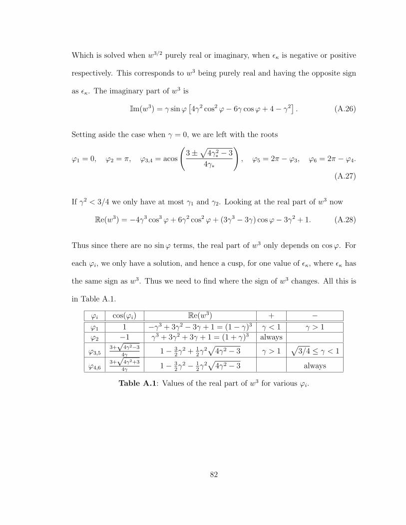
Which is solved when w3/2 purely real or imaginary, when εκ is negative or positive
respectively. This corresponds to w3 being purely real and having the opposite sign
as εκ. The imaginary part of w3 is
Im(w3) = γ sinϕ[4γ2 cos2 ϕ− 6γ cosϕ+ 4− γ2
]. (A.26)
Setting aside the case when γ = 0, we are left with the roots
ϕ1 = 0, ϕ2 = π, ϕ3,4 = acos
(3±
√4γ2
∗ − 3
4γ∗
), ϕ5 = 2π − ϕ3, ϕ6 = 2π − ϕ4.
(A.27)
If γ2 < 3/4 we only have at most γ1 and γ2. Looking at the real part of w3 now
Re(w3) = −4γ3 cos3 ϕ+ 6γ2 cos2 ϕ+ (3γ3 − 3γ) cosϕ− 3γ2 + 1. (A.28)
Thus since there are no sinϕ terms, the real part of w3 only depends on cosϕ. For
each ϕi, we only have a solution, and hence a cusp, for one value of εκ, where εκ has
the same sign as w3. Thus we need to find where the sign of w3 changes. All this is
in Table A.1.
ϕi cos(ϕi) Re(w3) + −ϕ1 1 −γ3 + 3γ2 − 3γ + 1 = (1− γ)3 γ < 1 γ > 1
ϕ2 −1 γ3 + 3γ2 + 3γ + 1 = (1 + γ)3 always
ϕ3,53+√
4γ2−3
4γ1− 3
2γ2 + 1
2γ2√
4γ2 − 3 γ > 1√
3/4 ≤ γ < 1
ϕ4,63+√
4γ2+3
4γ1− 3
2γ2 − 1
2γ2√
4γ2 − 3 always
Table A.1: Values of the real part of w3 for various ϕi.
82
Appendix B
Work Towards the Mixed Penrose
Inequality
B.1 Purpose
This appendix is a record of my attempts towards solving what we have been calling
the “Mixed Penrose Inequality.” The desired conjecture is as follows:
Conjecture B.1.1 (Mixed Penrose Inequality). Let (M, g) be an asymptotically flat
manifold with outer minimizing boundary Σ and negative mass singularities pi. Also
assume that (M, g) has nonnegative scalar curvature. Then
mADM(G) ≥√|Σ|16π
−
(∑i
mR(pi)2/3
)3/2
. (B.1)
The exponent on the negative point mass singularity term comes from consoli-
83
dating the integrals for the masses as follows (assuming they are regular):
−
(∑i
mR[pi]2/3
)3/2
= −
∑i
[1
4
(1
π
∫Σi
ν(ϕ)4/3da
)3/2]2/3
3/2
(B.2)
= −
(∑i
1
43/2
1
π
∫Σi
ν(ϕ)4/3da
)3/2
(B.3)
= −1
4
(1
π
∫∪iΣi
ν(ϕ)4/3da
)3/2
. (B.4)
This has so far been out of our reach. As a first case we have been working on
a reduced conjecture which assumes the singularity and black hole have equal and
opposite masses. Then all that is expected is that the ADM mass is positive.
Conjecture B.1.2. Let (M, g) be an asymptotically flat 3-manifold, with minimal
boundary Σ and negative mass singularity p of opposite mass. Also assume that
(M, g) has nonnegative scalar curvature. Assume that p can be resolved by a har-
monic conformal factor ϕ so that (M, g) is asymptotically flat, Σ is still minimal,
and Π, the resolution of p, is minimal as well. We can assume that ϕ = 1 at infinity,
ϕ = 0 only on Π, ν(ϕ) = 1 on Π, and ν(ϕ) = 0 on Σ.
Then the ADM mass of (M, g) is non-negative.
There are three methods we have for proving Penrose style theorems. Inverse
mean curvature flow, as in [7], which only takes into account a single horizon or
singularity, so probably won’t be helpful here. Bray’s conformal flow of metrics as in
[5] is the method we worked most with. Lastly, Bray’s Minimal Surface Resolution
technique used in [6], might also be useful, however to use it, we would need to adapt
84
it to accommodate the black holes. Furthermore, one of the steps in its proof is not
yet complete.
B.2 Effects of Harmonic Conformal Flow
The basic idea here is to use a harmonic conformal flow on the model space (M, g),
which is equivalent to a harmonic conformal flow on the actual space (M, g).
If we look at a flow on ϕ, and set ψ = ddtϕ, then we can look at the changes to
the various quantities. If we set m to be the ADM mass, M to be the mass of the
black hole, and N to the mass of the negative mass singularity.
N(Π) = −1
4
(1
π
∫Π
ν(ϕ)4/3dA
)3/2
(B.5)
M(Σ) =
√∣∣Σ∣∣16π
(1− 1
16π
∫Σ
H2dA
)(B.6)
For a first estimate we will look at the rate of change at time zero for initial ψ. First
we look at Π. A direct calculation shows
N(Π) = −3
8
(1
π
∫Π
ν(ϕ)4/3dA
)1/2(1
π
∫Π
ν(ϕ)1/3
[4
3ν(ψ) +Hψ
]dA
). (B.7)
Under the assumption that we are working at t = 0, we can put in the known
information about ϕ to get:
N(Π) = −3
2
(1
π
∫Π
ν(ϕ)4/3dA
)1/2(1
π
∫Π
ν(ϕ)1/3
[4
3ν(ψ) +Hψ
]dA
)(B.8)
= N(Π)
∫Π
2ν(ψ) + 32HψdA∫
ΠdA
. (B.9)
85
If Π is minimal as well, we can drop the H term. We can also drop this term if we
assume that ψ = 0 on Π. Likewise we can compute the change to M as
M(Σ) =
√1
4π
(∫Σ
ϕ4dA
)−1/2(∫Σ
ψϕ3dA
)(B.10)
= M(Σ)
∫Σ
2ψϕ3dA∫Σϕ4dA
. (B.11)
The integral of H2 term drops out since H is zero. We are also concerned with the
change in the ADM mass of the manifold. We can measure that with the integral of
the flux across a sphere at infinity, since this will measure the 1/r term of ψ. (Here
we assume that ψ = 0 at infinity.) Since the harmonic functions have constant flux,
we know that the flux across Σ and Π will also give us the 1/r term for ψ. Thus the
change in m is given by
m =1
4π
(∫Σ
∇(ψ) · ν dA+
∫Π
∇(ψ) · ν dA)
(B.12)
=1
4π
(∫Σ
ν(ψ)dA+
∫Π
ν(ψ)dA
)(B.13)
Adding these together, the quantity we want to decrease is the mass surplus X,
X = m−M −N (B.14)
X = m− M − N (B.15)
=1
4π
(∫Σ
ν(ψ)dA+
∫Π
ν(ψ)dA
)− (B.16)
M
(∫Σ
2ψϕ3dA∫Σϕ4dA
)−N
(∫Π
2ν(ψ) + 32HψdA∫
ΠdA
). (B.17)
If we can flow so that this decreases until N (or M) is zero, then we can apply the
Penrose (NPMS) inequality to get that X ≥ 0 at this time, hence X ≥ 0 at t = 0,
86
and we are done. At this point we tried different boundary conditions to accomplish
this.
B.2.1 Boundary Conditions 1
For a first try, set ψ by the boundary conditions ψ = 0 at infinity, ψ = −α2
Rϕ4Rϕ3 on
Σ, with both integrals over Σ, and ψ = 0 and ν(ψ) = −β2
on Π. This gives a value
for X of
X =1
4π
∫Σ
ν(ψ)dA− β
8π|Π| − βM − αN. (B.18)
B.2.2 Boundary Conditions 2
As a second try, we can look at the boundary conditions, ψ = 0 at infinity, ψ = α
on Σ, ν(ψ) = β on Π, where we choose α to be −R
ϕ4
2R
ϕ3 , and pick β so that m is zero.
This means that the flux of ψ through the two surfaces is zero.
B.2.3 Unknown Boundary Conditions
Trying the boundary conditions ψ = 0 on Π and at infinity while we leave the
boundary conditions of ψ on Σ up in the air for now, except that we want ψ < 0
and ν(ψ) > 0. If we set S to be a large sphere at infinity, then m will be given by
14π
∫Sν(ψ), with ν being the outward pointing normal for all surfaces. Then since ψ
is harmonic we know that∫S
ν(ψ) +
∫Σ
ν(ψ) +
∫Π
ν(ψ) = 0 (B.19)
87
Now we will calculate what we get for N and for∫
Πν(ψ) for different values of ν(ψ).
Set ν(ϕ) = c. Solving the formula for N for |Π| we get
N = −1
4
(1
π
∫Π
ν(ϕ)4/3dA
)3/2
(B.20)
= −1
4
1
π3/2|Π|3/2 ν(ϕ)2 (B.21)
|Π| =(−4π3/2N/c2
)2/3(B.22)
= 24/3πN2/3c−4/3. (B.23)
With this in hand we can compute N .
N = −3
8
(1
π
∫Π
ν(ϕ)4/3dA
)1/2(1
π
∫Π
4
3ν(ϕ)1/3ν(ψ)dA
)(B.24)
= −|Π|1/2
2π3/2c
(∫Π
ν(ψ)dA
)(B.25)
= −1
2
(22/3π1/2N1/3c−2/3
) 1
π3/2c
(∫Π
ν(ψ)dA
)(B.26)
= −2−1/3π−1N1/3c1/3
(∫Π
ν(ψ)dA
). (B.27)
If we choose c = − 132N
. Then
N = −2−1/3π−1N1/3c1/3
(∫Π
ν(ψ)dA
)(B.28)
= 2−1/3π−1N1/3
(1
32N
)1/3(∫Π
ν(ψ)dA
)(B.29)
=1
4π
(∫Π
ν(ψ)dA
). (B.30)
Thus m − N is equal to 14π
(∫Πν(ψ)dA+
∫Sν(ψ)dA
). Hence, in order to prove
monotonicity of X, we only need to show that 4πM ≥ −∫
Σν(ψ)dA.
88
Conjecture B.2.1. Let M be an asymptotically flat manifold with positive curvature.
Let M contain negative point mass singularities pi and black holes Σj. Assume that
the pi can be resolved with a function ϕ on M so that ϕ = 1 at infinity, ν(ϕ) = 0
on Σ, ϕ = 0 on Π, ν(ϕ) = − 132N
on Π, where N is the mass of the pi, summed
appropriately, and Π is minimal. Then
mADM(M) ≥
(∑i
mH(Σi)2
)1/2
−
(∑i
|mR(pi)|2/3
)3/2
. (B.31)
This requires only the following conjecture:
Conjecture B.2.2. Under the conditions of conjecture B.2.1, let ψ be the harmonic
function on M so that ψ = 0 at infinity, ν(ψ) = −1 on Σ, and ψ = 0 on Π. Then
√4π
(∫Σ
ϕ4dA
)−1/2(∫Σ
ψϕ3dA
)≥∫
Σ
ν(ψ)dA (B.32)
Removing this from context gives the following conjecture:
Conjecture B.2.3. Let M be an asymptotically flat manifold with positive scalar
curvature. Let M have two sets of boundary Σ and Π. Let ϕ be a function so that
ϕ = 0 on Π, ν(ϕ) = 0 on Σ, ϕ = 1 at ∞ and ∆ϕ = 0. Furthermore assume that
ν(ϕ) =√
π
512|Π|1/2 on Π. Then let ψ be the harmonic function defined by ψ = 0 on Π,
ψ = 0 at ∞. We can choose our boundary conditions for ψ on Σ so that
0 ≥√
4π
(∫Σ
ϕ4dA
)−1/2(∫Σ
ψϕ3dA
)≥ −
∫Σ
ν(ψ)dA (B.33)
Of course this would require that ν(ψ) > 0 on Σ and ψ < 0 on Σ.
If we recast this on the original manifold M , we get the following statement:
89
Conjecture B.2.4. Let (M, g) be an asymptotically flat 3-manifold, with minimal
boundary Σ and negative mass singularity p of opposite mass. Also assume that
(M, g) has non-negative scalar curvature. Assume that p can be resolved by a har-
monic conformal factor ϕ so that (M, g) is asymptotically flat, Σ is still minimal and
Π, the resolution of p, is minimal as well. We can assume that ϕ = 1 at infinity,
ϕ = 0 only on Π, ν(ϕ) = 1 on Π, and ν(ϕ) = 0 on Σ.
Then there are boundary conditions, X, on Σ so that if ψ is the solution to
∆(ψ/ϕ) = 1, with boundary values 0 at ∞ and p, and X on Σ, then
0 ≥√
4π∣∣Σ∣∣(∫
Σ
ψ
ϕdA
)≥ −
∫Σ
ν(ψ)
ϕ4dA. (B.34)
What these X boundary conditions might be we have been unable to ascertain.
90
Bibliography
[1] R. Arnowitt, S. Deiser, and C. Misner, Coordinate invariance and energy ex-pressions in general relativity., Physical Review 122 (1961), 997–1006.
[2] Robert Bartnik, New definition of quasilocal mass, Physical Review Letters 62(1989), 2346–2349.
[3] Hubert Bray, On negative point mass singularities, in preparation, 2007.
[4] Hubert Bray and Pengzi Miao, On the capacity of surfaces in manifolds withnonnegative scalar curvature, 2007, http://arxiv.org/abs/0707.3337.
[5] Hubert L. Bray, Proof of the Riemannian Penrose inequality using the positivemass theorem, Journal of Differential Geometry 59 (2001), 177–2677.
[6] , Negative point mass singularities in general relativity,http://www.newton.cam.ac.uk/webseminars/pg+ws/2005/gmr/0830/bray/,August 2005.
[7] G. Huisken and T. Ilmanen, The inverse mean curvature flow and the Rieman-nian Penrose inequality., Journal of Differential Geometry 59 (2001), 353–437.
[8] Hideo Kodama and Wataru Hikida, Global structure of the Zippoy–Voorhees–Weyl spacetime and the δ = 2 Tomimatsu-Sato spacetime, Classical and Quan-tum Gravity 20 (2003), 5121–5140.
[9] Arlie O. Petters, Harold Levine, and Joachim Wambsganss, Singularity theoryand gravitational lensing, Birkhauser, 2001.
[10] Jeffrey Streets, Quasi-local mass functionals and generalized inverse mean cur-vature flow, Omitted from published version, 2006.
[11] Kip S. Thorne, Charles W. Misner, and John Archibald Wheeler, Gravitation,W. H. Freeman, 1973.
[12] Robert M. Wald, General relativity, The University of Chicago Press, 1984.
91
Biography
Nicholas Philip Robbins is from Merrick, New York. He received a BA from Swarth-
more College in 2001 with High Honors with the Major in Mathematics and the
Minor in Ancient History. He received a MS from Duke University in 2003 in Math-
ematics. He will be a Visiting Assistant Professor of Mathematics at St. Mary’s
College of Maryland for 2007–2008.
92