negative-exponent power functions - free math...

power functions, negative-coefficient

Chapter 6

Negative-Exponent PowerFunctions

Input-Output Pairs, 165 – Normalized Input-Output Rule, 168 – LocalGraph Near ∞, 171 – Types of Local Graphs Near ∞, 186 – The EssentialQuestion, 187 – Local Graph near 0, 189 – Types of Local Graphs Near 0,195 – Essential Bounded Graph, 196 – Existence of Notable Inputs, 197 –Essential Global Graph, 199 – Types of Global Graphs, 201.

Negative-exponent power functions are functions that divide a givennumber, called the coefficient, by a given number of copies of the input.More precisely:• The coefficient can be any finite number.• The exponent, which can be any negative counting number, says what

the function will do tho the coefficient::– The − sign of the exponent says that the coefficient is to be divided

by the copies of the input.EXAMPLE 1.

xFLOP−−−−−−→ FLOP (x) = (+8 273.1)x−5

= +8 273.1x · x · x · x · x︸︷︷︸

5 copies of x

– The size of the exponent gives the number of copies of the input thatare to be used.

163

164 CHAPTER 6. NEGATIVE-EXPONENT POWER FUNCTIONS

power functionpower function, regular

EXAMPLE 2.

xFLIP−−−−−−→ FLIP (x) = (+8 273.1)x−5

= +8 273.1x · x · x · x · x︸︷︷︸

5 copies of x

1. Occasionally, we will be able to make statements that are true both ofpositive-exponent power functions and of negative-exponent power functionsand zero-power functions so, it will be convenient to lump them all togetherand use power function to mean a function that can be a positive-exponentpower function or a negative-exponent power function or a zero-power func-tion. In other words, the exponent in a power function can be any signedcounting number.EXAMPLE 3. All of the following:• the regular positive-exponent power function

xFLIP−−−−−−→ FLIP (x) = (−13.44)x+6

• the exceptional positive-exponent power function

xFLIP−−−−−−→ FLIP (x) = (−13.44)x+1

• the zero-power function

xBLOP−−−−−−→ FLOP (x) = (+8 273.1)x0

• the negative-exponent power function

xFLOP−−−−−−→ FLOP (x) = (+8 273.1)x−5

are power functions.2. Recall, though, that in Chapter 4, we called regular positive-power

functions those positive-power functions whose exponent is different from +1as distinguished from the exceptional power functions, that is those powerfunctions whose exponent is either +1 or 0.Quite often, we will be able to make statements that are true both of regularpositive-exponent power functions and of negative-exponent power functionsbut not of the exceptional power functions, that is those power functionswhose exponent is either +1 or 0.So it will be convenient to call regular power functions those powerfunctions whose exponent is any signed counting number except +1 and0. Still in other words, regular power functions are either regular positive-exponent power functions or negative-exponent power functions.

6.1. INPUT-OUTPUT PAIRS 165

EXAMPLE 4. Both the regular positive-exponent power function

xFLIP−−−−−−→ FLIP (x) = (−13.44)x+6

and the negative-exponent power function

xFLOP−−−−−−→ FLOP (x) = (+8 273.1)x−5

are regular power functions but neither the exceptional positive-exponent power func-tion

xBLIP−−−−−−→ FLIP (x) = (−13.44)x+1

nor the zero-power function

xBLOP−−−−−−→ FLOP (x) = (+8 273.1)x0

are regular power functions.3. The reason we continue our investigation of Algebraic Functions

with negative-exponent power functions, and the reason these are also ex-tremely important, is that:i. negative-exponent power functions are almost as simple as positive-exponentpower functions,ii. negative-exponent power functions already exhibit the local qualitativefeatures that we discussed earlier and in terms of which Rational Func-tions will be investigated in Part Three of this text,iii. negative-exponent power functions are the other “building blocks” interms of which we will “deconstruct” Rational Functions in Part Threeof this text.

6.1 Input-Output PairsAs with any function, given the input-output rule, in order to get the outputfor a given input we must:

i. Read and write what the input-output rule says,ii. Replace x in the given input-output rule by the given inputiii. Identify the resulting specifying phrase.

EXAMPLE 5. Given the input-output rule

xFLOP−−−−−−→ FLOP (x) = (+5273.1) · x−5

and given the input −3, in order to get the input-output pair, we proceed as follows..


a. To get the output:i. We read and write what the input-output rule says:

• The input-output rule reads:

“The output of FLOP is obtained by dividing +5273.1 by 5 copies of the input.”• We write

xFLOP−−−−−−→ FLOP (x) = (+5, 273.1)x−5

= +5, 273.1x · x · x · x · x︸︷︷︸

5 copies of x

ii. We indicate that x is about to be replaced by the given input −3

x∣∣∣x:=−3

FLOP−−−−−−−−−→ FLOP (x)∣∣∣x:=−3

= +5, 273.1x · x · x · x · x︸︷︷︸

5 copies

∣∣∣x:=−3

which gives us the following specifying-phrase

= +5, 273.1(−3) · (−3) · (−3) · (−3) · (−3)︸︷︷︸

5 copies

iii. We identify the specifying-phrase

= +5, 273.1−243

= −21.7

Without the comments, here is how things should look like once all done:

x|x:=−3FLOP−−−−−−−−−→ FLOP (x)|x:=−3 = +5, 273.1

x · x · x · x · x

∣∣∣∣x:=−3

= +5, 273.1(−3) · (−3) · (−3) · (−3) · (−3)

= +5, 273.1−243

= −21.7

b. Depending on the circumstances, we can then write:

−3 FLOP−−−−−−→ −21.47

6.1. INPUT-OUTPUT PAIRS 167

orFLOP (−3) = −21.47

or(−3,−21.47) is an input-output pair for the function FLOP

.EXAMPLE 6. Given the input-output rule

xFLOP−−−−−−→ FLOP (x) = (+112)x−4

and given the input −5, in order to get the input-output pair, we proceed as follows.:a. To get the output:

i. We read and write what the input-output rule says:• The input-output rule reads:

“The output of FLOP is obtained by dividing +112 by 4 copies of the input.”• We write

xFLOP−−−−−−→ FLOP (x) = (+112)x−4

= +112x · x · x · x︸︷︷︸4 copies of x

ii. We indicate that x is to be replaced by the given input +2

x∣∣∣x:=+2

FLOP−−−−−−−−−→ FLOP (x)∣∣∣x:=+2

= +112x · x · x · x︸︷︷︸4 copies of x

∣∣∣x:=+2

which gives us the following specifying-phrase

= +112(+2) · (+2) · (+2) · (+2)︸︷︷︸

4 copies of +2

iii. We identify the specifying-phrase

= +7

Without all the comments, here is how getting the output should look like once it is all


features, of input-outputrule

sign, of the exponentparity, of the exponentsign, of the coefficienttypeNEPNENNOPNON

done:

x|x:=+2FLOP−−−−−−−−−→ FLOP (x)|x:=+2 = (+112)x−4∣∣

x:=+2

= +112x · x · x · x

∣∣∣∣x:=+2

= +112(+2) · (+2) · (+2) · (+2)

= +7

b. Depending on the circumstances, we can then write:

+2 FLOP−−−−−−→ +7

orFLOP (+2) = +7

or(+2,+7) is an input-output pair for the function FLOP

6.2 Normalized Input-Output Rule

The input-output rule of a negative-exponent power function thus has a num-ber of features but since we will be mostly dealing with qualitative investi-gations, these features will not be equally important to us.

1. As with positive-exponent power functions, the three features thatwill be important to us are:• The sign of the exponent which, for negative-exponent power functions,

is −,• The parity of the exponent which can be even or odd depending on

whether the number of copies is even or odd,• The sign of the coefficient which can be + or −.From our point of view,• The size of the coefficient will not be an important feature to us because

of the requirement in the definition of a negative-exponent power functionat the start of this chapter that the coefficient be a finite number.

• The size of the exponent will not be an importaht feature to us becausethe plain number of copies will not matter from our qualitative viewpoint.2. From the qualitative viewpoint that we will be taking, there will there-

fore be four types of negative-exponent power functions:

6.2. NORMALIZED INPUT-OUTPUT RULE 169

normalizeSign exponent Parity exponent Sign coefficient TYPE

−Even

+ NEP− NEN

Odd+ NOP− NON

EXAMPLE 7. The function PLIP whose input-output rule is

xPLIP−−−−−−→ PLIP (x) = ((+6836))x−7

= +6 836x · . . . · x︸︷︷︸7 copies of x

is a power function whose input-output rule has the following features• The exponent is Negative,• The exponent is Odd.• The coefficient is Positive,So, the power function PLIP is of type NOP .EXAMPLE 8. The function MILK whose input-output rule is

xMILK−−−−−−→MILK(x) = (+4 500)x−6

= +4 500x · . . . · x︸︷︷︸6 copies of x

is a power function whose input-output rule has the following features• The exponent is Negative,• The exponent is Even.• The coefficient is Positive,So, the power function MILK is of type NEP .

3. In fact, as with positive-exponent power functions, a negative-exponentpower function being given by an input-output rule, what we will do is tonormalize the input-output rule, that is we will strip the exponent and thecoefficient of all the information that is irrelevant from our qualitative pointof view:• We will normalize the exponent as follows:

If the exponent is: we will normalize it to:Negative Even − evenNegative Odd − odd

• We will normalize the coefficient as follows:


If the coefficient is: we will normalize it to:Positive +1Negative −1

EXAMPLE 9. The function CRIC whose input-output rule is

xCRIC−−−−−−→ CRIC(x) = (−345)x−15

=−345x · . . . · x︸︷︷︸15 copies of x

will be normalized to

xCRIC−−−−−−→ CRIC(x) = (−1)x−odd

=−1

x · . . . · x︸︷︷︸odd number of copies of x

EXAMPLE 10. The function CRIP whose input-output rule is

xCRIC−−−−−−→ CRIP (x) = (+562)x−12

=+562x · . . . · x︸︷︷︸12 copies of x

will be normalized to

xCRIP−−−−−−→ CRIP (x) = (−1)x−even

=−1

x · . . . · x︸︷︷︸even number of copies of x

4. So, the four types of negative-exponent power functions have the fol-lowing normalized input-output rules:

TYPE Normalized input-output rule

NEP xNEP−−−−−→ NEP (x) = (+1)x− even

NEN xNEN−−−−−→ NEN(x) = (−1)x− even

NOP xNOP−−−−−→ NOP (x) = (+1)x− odd

NON xNON−−−−−→ NON(x) = (−1)x− odd

6.3. LOCAL GRAPH NEAR ∞ 171

RECIPROCALreciprocal function

5. As with regular positive-exponent power functions, because of our useof even and odd as exponent, the above are not global input-output rules offunctions but only of types of functions and we often will use gauge powerfunctions.In particular, we will often use, for many purposes, the gauge power functionRECIPROCAL specified by the global input-output rule

xRECIPROCAL−−−−−−−−−−−−−−−→ RECIPROCAL(x) = x−1

and we will often speak of the reciprocal functionIt is of course a prototype for power functions of type NOP but rarely usedas such, perhaps because there is no standard name for a prototype forfunctions of type NEP .

LOCAL ANALYSIS

6.3 Local Graph Near ∞

The way we will get the local graph near∞ from the input-output rule in thecase of a negative-exponent power function will be almost exactly the sameas what we did in the case of a positive-exponent power function. Again,there are several possible approaches:

1. We could use a bare hands approach and proceed “from scratch”, thatis in a manner based uniquely on:• The definition of “large-in-size”, namely on the fact that copies of a

number that is large-in-size multiply to a result that is large-in-size• The fact that a finite coefficient divided by a result that is large-in-size

gives an output that is small-in-size• The “rule of signs” for multiplication

+ −+ + −− − +

namely on the fact that:– multiplying copies of a positive input will result in a positive result

no matter what the number of copies is,– multiplying copies of a negative input will result:

in a positive result if the number of copies is evenin a negative result if the number of copies is odd


EXAMPLE 11. Given the function NADE whose input-output rule is

xNADE−−−−−−−→ NADE(x) = (−8)x−5

we want to find the local graph near ∞.i. We normalize the input-output rule to

xNADE−−−−−−−→ NADE(x) = (−1)x−odd

ii. We look for the place of the local graph near ∞:• To get the place of the local graph near +∞, we compute the output for inputs

that are +large:

x∣∣∣x:=+large

NADE−−−−−−−→ NADE(x)∣∣∣x:=+large

= (−1)x−odd∣∣∣x:=+large

= (−1)(+large)−odd

= −1(+large) · . . . · (+large)︸︷︷︸odd number of copies of +large

and since,– by the Definition of large, copies of large multiply to large– by the Rule of Signs, any number of copies of + multiply to +

= −1+large

and, by the fact that a finite coefficient divided by a result that is large-in-sizegives an output that is small-in-size,

= −small

and so we have that

NADE(+large) = −small

So, we have that the place of the local graph near +∞ is

Input Ruler

Output Ruler

(

)

Screen

0–

+∞–∞


• To get the place of the local graph near −∞, we compute the output for inputsthat are −large:

x∣∣∣x:=−large

NADE−−−−−−−→ NADE(x)∣∣∣x:=−large

= (−1)x−odd∣∣∣x:=−large

= −1(−large) · . . . · (−large)︸︷︷︸odd number of copies of −large

and since,– by the Definition of large, copies of large multiply to large– by the Rule of Signs, an odd number of copies of − multiply to −

= −1−large

and, by the fact that a finite coefficient divided by a result that is large-in-sizegives an output that is small-in-size,

= +small

and so we have that

NADE(−large) = +small

So, we have that the place of the local graph near −∞ is

Input Ruler

Output Ruler

)

(Screen

+∞–∞

0+

Altogether, we found that the place of the local graph near ∞ is:

Input Ruler

Output Ruler

) (

()

Screen

0–

+∞–∞

0+

iii. We look for the shape of the local graph near∞ which involves having to computewith specific inputs.


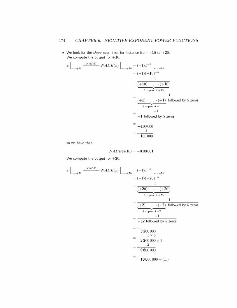
• We look for the slope near +∞, for instance from +10 to +20.We compute the output for +10:

x∣∣∣x:=+10

NADE−−−−−−−→ NADE(x)∣∣∣x:=+10

= (−1)x−5∣∣∣x:=+10

= (−1)(+10)−5

= −1(+10) · . . . · (+10)︸︷︷︸

5 copies of +10

= −1(+1) · . . . · (+1)︸︷︷︸

5 copies of +1

followed by 5 zeros

= −1+1 followed by 5 zeros

= −1+100 000

= − 1100 000

so we have that

NADE(+10) = −0.00 001

We compute the output for +20:

x∣∣∣x:=+20

NADE−−−−−−−→ NADE(x)∣∣∣x:=+20

= (−1)x−5∣∣∣x:=+20

= (−1)(+20)−5

= −1(+20) · . . . · (+20)︸︷︷︸

5 copies of +20

= −1(+2) · . . . · (+2)︸︷︷︸

5 copies of +2

followed by 5 zeros


= − 13 200 000

= − 1× 33 200 000× 3

= − 39 600 000

= − 310 000 000 + (...)


= − 310 000 000 + (...)

so we have that

NADE(+20) = −0.00 000 03 + (...)

Now we compute the slope from +10 to +20:NADE(+20)−NADE(+10)

(+20)− (+10) = [−0.00 000 03 + (...)]− [−0.00 001](+20)− (+10)

= −0.00 000 03 + (...) + 0.00 001+20− 10

= +0.00 001 + (...)+10

= +0.00 000 1 + (...)+1

= +0.00 000 1 + (...)1

= +0.00 000 11 + (...)

The slope near +∞ is thus small-in-size and positive:Output Ruler

)

Screen

0–

slope = 0.000 001 +1

+ (…)

Input Ruler(

+∞–∞

+10+20

–0.00 000 03 + (…)

–0.00 001 + (…)

• We look for the slope near −∞ and compute, say, the slope from −20 to −10.We compute the output for −20::

x∣∣∣x:=−20

NADE−−−−−−−→ NADE(x)∣∣∣x:=−20

= (−1)x−5∣∣∣x:=−20

= (−1)(−20)−5

= −1(−20) · . . . · (−20)︸︷︷︸

5 copies of −20

= −1(−2) · . . . · (−2)︸︷︷︸

5 copies of −2

followed by 5 zeros


= −1−32 followed by 5 zeros

= −1−3 200 000

= + 13 200 000

= + 1× 33 200 000× 3

= + 39 600 000

= + 310 000 000 + (...)

= + 310 000 000 + (...)

so we have that

NADE(−20) = +0.00 000 03 + (...)

We compute the output for −10:

x∣∣∣x:=−10

NADE−−−−−−−→ NADE(x)∣∣∣x:=−10

= (−1)x−5∣∣∣x:=−10

= (−1)(−10)−5

= −1(−10) · . . . · (−10)︸︷︷︸

5 copies of −10

= −1(−1) · . . . · (−1)︸︷︷︸

5 copies of −1

followed by 5 zeros


= −1−100 000

= + 1100 000

so we have that

NADE(−10) = +0.00 001

Now we compute the slope from −20 to −10:

NADE(−10)−NADE(−20)(−10)− (−20) = [+0.00 001]− [+0.00 000 03 + (...)]

(−10)− (−20)


= +0.00 001− 0.00 000 03 + (...)−10 + 20

= +0.00 001 + (...)+10

= +0.00 000 1 + (...)+1

= +0.00 000 1 + (...)1

= +0.00 000 11 + (...)

and we get again that the slope is small-in-size and positive:

Input Ruler

Output Ruler

)

(Screen

+∞–∞

0+

slope = 0.000 001 +1

+ (…)

• Altogether, the slope near ∞ is:

Input Ruler

Output Ruler

) (

()

Screen

0–

+∞–∞

0+

• We look for the concavity near +∞ by computing, say, the slope from +20 to +30and comparing it with the slope from +10 to +20 (which we already computedabove).We already computed the output for +20

NADE(+20) = −0.00 000 03 + (...)

We compute the output for +30:

x∣∣∣x:=+30

NADE−−−−−−−→ NADE(x)∣∣∣x:=+30

= (−1)x−5∣∣∣x:=+30

= (−1)(+30)−5

= −1(+30) · . . . · (+30)︸︷︷︸

5 copies of +30


= −1(+3) · . . . · (+3)︸︷︷︸

5 copies of +3

followed by 5 zeros


= −1+24 300 000

= − 124 300 000

= − 1× 424 300 000× 4

= − 497 200 000

= − 4100 000 000 + (...)

= − 4100 000 000 + (...)

so we have that

NADE(+30) = −0.00 000 004 + (...)

Now we compute the slope from +20 to +30:

NADE(+30)−NADE(+20)(+30)− (+20) = [−0.00 000 004 + (...)]− [−0.00 000 03 + (...)]

(+30)− (+20)

= −0.00 000 004 + (...) + 0.00 000 03 + (...)+10

= +0.00 000 03 + (...)+10

= +0.000 000 003 + (...)+1

= +0.000 000 03 + (...)1

= +0.000 000 031 + (...)

We compare the slope from +20 to +30 which we just computed to be

+0.000 000 031 + (...)

with the slope from +10 to +20 which we computed earlier to be

+0.00 000 11 + (...)

The slope from +20 to +30 is smaller-in-size than the slope from +10 to +20:


Input Ruler

Output Ruler

(

)

Screen

0–

+10–∞

+20+30

so that the concavity-sign near +∞ has to be ∩.• We look for the concavity near −∞ by computing, say, the slope from −30 to −20

and comparing it with the slope from −20 to −10 which we already computedabove.We compute the output for −30:

x∣∣∣x:=−30

NADE−−−−−−−→ NADE(x)∣∣∣x:=−30

= (−1)x−5∣∣∣x:=−30

= (−1)(−30)−5

= −1(−30) · . . . · (−30)︸︷︷︸

5 copies of −30

= −1(−3) · . . . · (−3)︸︷︷︸

5 copies of −3

followed by 5 zeros


= + 124 300 000

= + 1× 424 300 000× 4

= + 497 200 000

= + 4100 000 000 + (...)

= + 4100 000 000 + (...

so we have that

NADE(−30) = +0.00 000 004 + (...)

We already computed the output for −20:

NADE(−20) = +0.00 000 03 + (...)


Now we compute the slope from −30 to −20:

NADE(−20)−NADE(−30)(−20)− (−30) = [+0.00 000 03 + (...)]− [+0.00 000 004 + (...)]

(−20)− (−30)

= +0.00 000 03 + (...)− 0.00 000 004 + (...)−20 + 30

= +0.00 000 03 + (...)+10

= +0.00 000 003 + (...)+1

= +0.00 000 003 + (...)1

= +0.00 000 0031 + (...)

We compare the slope from −30 to −20 which we just computed to be

+0.00 000 0031 + (...)

with the slope from −20 to −10 which we computed earlier to be

+0.00 000 11 + (...)

The slope from −30 to −20 is smaller-in-size than the slope from −20 to −10:

–30–20–10

Input Ruler

Output Ruler

)

(Screen

+∞–∞

0+

so that the concavity-sign near −∞ has to be ∪.iv. So, finally, we have that the local graph of NADE near ∞ is

Input Ruler

Output Ruler

) (

()

Screen

0–

+∞–∞

0+

This bare hands approach, even though it would be very safe because it doesnot require any memorization, would be much too slow, in particular whenthe local graph near ∞ is not an end in itself but only a means towards


other ends such as, for instance, local features near∞, the essential boundedgraph or the essential global graph. It thus worthwhile to invest some timein making the case for some theorems and then invoke these theorems.

2. At one extreme, we could make the case for the followingTHEOREM 1 (Local Graph Near ∞). The local graphs near ∞ fornegative-exponent power functions are:

Input Ruler

Output Ruler

(

) Screen

+∞Input Ruler

Output Ruler

Input Ruler

Output Ruler

(

(

Screen

+∞Input Ruler

Output Ruler

)

Screen

–∞

Screen

–∞)

Even exponent Odd exponent

Positive coefficient Positive coefficient Negative coefficientNegative coefficient

)0+)

)0+

0– (0– 0+

0–

)

)

)–∞

)–∞

(+∞

(+∞

and then memorize the theorem and just invoke it in each particular case.

While this would of course be extremely fast, it would also be extremelydangerous in that we would be totally dependent on our remembering thetheorem perfectly with no chance of becoming aware of an error we mighthave made by misremembering the theorem and, even less, of recoveringfrom that error.

3. We will take a more reasonable, somewhat in-between approach whichwill use the following two theorems:

i. A theorem that says how the local graph near −∞ can be flipped fromthe local graph near +∞:THEOREM 2 (Local Place Near −∞). For a negative-exponent powerfunction, the local place near −∞ is obtained from the local place near +∞according to the parity of the exponent:

• When the exponent is even, the local place near −∞ is flipped horizon-tally from the local graph near +∞


forced Even exponent: horizontal-flip

Input Ruler

Output Ruler

) (

)

Screen

0+

+∞–∞Positive coefficient Negative coefficient

Input Ruler

Output Ruler

) (

Screen

+∞–∞

(0–

• When the exponent is odd, the local place near −∞ is flipped diagonallyfrom the local graph near +∞

Odd exponent: diagonal-flip

Negative coefficientPositive coefficient

Input Ruler

Output Ruler

) (

Screen

+∞–∞

0+

0–

)

)

Input Ruler

Output Ruler

) (

Screen

+∞–∞

)

)0+

0–

The case for the Local Place Near −∞ Theorem is entirely based onthe Rule of Signs and so the details of the case are left to the reader.ii. A theorem that says how the shape of the local graph of a negative-exponent power function is forced by the place.THEOREM 3 (Local Shape Near ∞). For negative-exponent powerfunctions, as inputs go towards ∞, the local graph near ∞ tends to becomehorizontal and so its shape is forced by the place as follows:

Input Ruler

Output Ruler

(

) Screen

+∞Input Ruler

Output Ruler

Input Ruler

Output Ruler

(

(

Screen

+∞Input Ruler

Output Ruler

)

Screen

–∞

Screen

–∞)

Even exponent Odd exponent

Positive coefficient Positive coefficient Negative coefficientNegative coefficient

)0+)0– (0– 0+ )

The case for the Local Shape Near ∞ Theorem is not much harder tomake since it follows essentially what we did in the bare hands approach but


is therefore somewhat lengthy and we will leave it to the Supplement.4. The procedure that we will be using will be the same as the one we

used for regular positive-exponent power functions:

i. Normalize the input-output rule,ii. Get the place of the local graph near +∞, by computing the output forinputs that are +large,iii. Get the place of the local graph near −∞ by using the Local PlaceNear −∞ Theorem (instead of computing the output for inputs that are−large),iv. Get the local graph near∞ by using the Local Shape Near ∞ The-orem (Instead of computing all these slopes).

EXAMPLE 12. Given the positive-exponent power function NATE whose input-outputrule is

xNATE−−−−−−→ NATE(x) = (−33.14159)x−12

= −33.14159x · . . . · x︸︷︷︸12 copies of x


xNATE−−−−−−→ NATE(x) = (−1)x−even

= −1x · . . . · x︸︷︷︸

even number of copies of x

ii. We compute the output for inputs that are +large to get the local place near +∞:

+large NATE−−−−−−→ NATE(+large) = (−1)(+large)−even

= −1(+large) · . . . · (+large)︸︷︷︸even number of copies of +large

and since,• by the Definition of large, copies of large multiply to large• by the Rule of Signs, any number of copies of + multiply to +

= −1+large

= −small


So, we have that the place of the local graph of NATE near +∞ is

Input Ruler

Input Ruler

Output Ruler

(

Screen

+∞

)0–

iii. Since the exponent is even, we get from the Local Place Near −∞ Theorem thatthe place of the local graph near −∞ is flipped horizontally from the local graph near+∞ to

Input Ruler

Output Ruler

) (

Screen

+∞–∞

(0–

iv. And then the Local Shape Near ∞ Theorem says that the local graph of NATEnear ∞ must be

Input Ruler

Output Ruler

) (

Screen

+∞–∞

(0–

EXAMPLE 13. Given the positive-exponent power function NAV E whose input-outputrule is

xNAV E−−−−−−−→ NAV E(x) = (−33.14159)x−7

= −33.14159x · . . . · x︸︷︷︸7 copies of x


xNAV E−−−−−−−→ NAV E(x) = (−1)x−odd

= −1x · . . . · x︸︷︷︸

odd number of copies of x


ii. We compute the output for inputs that are +large to get the local place near +∞:

+large NAV E−−−−−−−→ NAV E(+large) = (−1)(+large)−odd

= −1(+large) · . . . · (+large)︸︷︷︸odd number of copies of +large

and since,• by the Definition of large, copies of large multiply to large• by the Rule of Signs, any number of copies of + multiply to +

= −1+large

= −small

So, we have that the place of the local graph of NAV E near +∞ is

Input Ruler

Input Ruler

Output Ruler

(

Screen

+∞

)0–

iii. Since the exponent is odd, we get from the Local Place Near −∞ Theorem thatthe place of the local graph near −∞ is flipped diagonally from the local graph near+∞ to

( Input Ruler

Output Ruler

)

Screen

+∞–∞

0+0–

)

)

iv. And then the Local Shape Near ∞ Theorem says that the local graph of NAV Enear ∞ must be


( Input Ruler

Output Ruler

)

Screen

+∞–∞

0+0–

)

)

5. While the Arithmetic involved with the bare hands procedure isquite a bit harder with negative-exponent power functions than it was withpositive-exponent power functions, other than that, we saw that the familiar-ity with the procedures we acquired with positive-exponent power functionstransferred completely to negative-exponent power functions.

6.4 Types of Local Graphs Near ∞Proceeding in the same manner as above, we get the local graph near∞ foreach one of the four types of negative-exponent power function. They areshown in the table below as seen from two viewpoints:

i. As seen from “not too far”, that is we see the screen and only thepart of the local graph near ∞ that is near the transition, that is for inputsthat are large but not “that” large so that we can still see the slope and theconcavity.

ii. As seen from “faraway”. Indeed, in order to see really large inputs,we need to be “faraway” but then the parts of the local graph near ∞ thatwe see are essentially straight and vertical.

Input-output rule From “not too far” From “faraway”

xNEP−−−→ NEP (x) = +x−even

Output Ruler

Input Ruler

0

0 +∞–∞

–∞

+∞

Screen

Continued on next page

6.5. THE ESSENTIAL QUESTION 187


xNEN−−−→ NEN(x) = −x−even

Output Ruler

Input Ruler

0

0 +∞–∞

–∞

+∞

Screen

xNOP−−−→ NOP (x) = +x−odd

Output Ruler

Input Ruler

0

0 +∞–∞

–∞

+∞

Screen

xNON−−−→ NON(x) = −x−odd

Output Ruler

Input Ruler

0

0 +∞–∞

–∞

+∞

Screen

6.5 The Essential QuestionWe now need to find out if the outlying graph includes just the local graphnear ∞ or if it also includes local graph(s)) near ∞-height inputs.

1. In other words, before we can proceed, we need to answer the Es-sential Question:

• Do all bounded inputs have bounded outputs (for some extent of theoutput ruler)

or• Is there one (or more) bounded input that is an∞-height input, namely

whose nearby inputs have infinite outputs (no matter what the extentof the output ruler)?

Since, in the case of negative-exponent power functions, the coefficient is tobe divided by copies of the input, the input 0 would immediately seem to


create a difficulty since we cannot divide by 0. The Essential Question,though, asks whether nearby inputs have infinite outputs so that the answeris:THEOREM 4 (Height). For negative-exponent power functions, 0 hasinfinite height, that is nearby inputs have infinite height.

Making the case is based on the fact that dividing a finite coefficient bycopies of a small input results in a large output.EXAMPLE 14. Given the function NYK whose input-output rule is

xMYK−−−−−−→ NYK(x) = +20x+5

and given an input near 0, that is given a small input, we compute the output:

x∣∣∣x:=−small

NY K−−−−−−→ NYK(x)∣∣∣x:=−small

= (+20)x−5∣∣∣x:=−small

= +20x · . . . · x︸︷︷︸

odd number of copies of x

∣∣∣∣x:=−small

= +20(−small) · . . . · (−small)︸︷︷︸odd number of copies of −small

= +20−small

= −large

2. So the outlying graph of a negative-power function does not includejust the local graph near ∞ but also the local graph near 0.This affects the “story line” for negative-exponent power functions which,until now, was exactly the same as the “story line” for positive-power func-tions because now there is a major difference:• In the case of positive-exponent power functions, once we had answered

the essential question (in the negative), the “story line” proceeded withgetting:i. the essential bounded graph on the basis of the local graph near ∞,ii. the existence of notable input(s) on the basis of the essential boundedgraph,iii. the local graph near 0 on the basis of 0 being the most likely possi-bility for being the notable input,iv. the different types of local graphs near 0.

6.6. LOCAL GRAPH NEAR 0 189

• In the case of negative-exponent power functions, once we have answeredthe essential question (in the positive), we have no choice and the “storyline” must proceed with gettingi. the local graph near 0 on the basis of 0 being an ∞-height input,ii. the different types of local graphs near 0,iii. the essential bounded graph on the basis of the local graph near ∞and the local graph near 0,iv. the existence of notable input(s) on the basis of the essential boundedgraph,After which, just as with positive-power functions, we will conclude withthe essential global graphs.

6.6 Local Graph near 0The way we will get the local graph near 0 will follow very closely the waywe got the local graph near ∞ as well as the way we got the local graphsnear ∞ and near 0 in the case of positive-power functions.

1. We could use a bare hands approach, that is proceed “from scratch”,that is in a manner based uniquely on:• The definition of “small-in-size”, namely on the fact that copies of a

number that is small-in-size multiply to a result that is small-in-size• The fact that a finite coefficient divided by a result that is small-in-size

gives an output that is large-in-size• The “rule of signs” for multiplication

+ −+ + −− − +

namely on the fact that:– multiplying copies of a positive input will result in a positive result

no matter what the number of copies is,– multiplying copies of a negative input will result:

in a positive result if the number of copies is evenin a negative result if the number of copies is odd

This approach, even though it would be very safe because it does not requireany memorization, would be much too slow, in particular when the localgraph near 0 is not an end in itself but only a means towards other endssuch as, for instance, local features near 0, the essential bounded graph orthe essential global graph.

2. At the other extreme, we could just make the case for the following


THEOREM 5 (Local Graph Near 0). The local graphs near 0 fornegative-exponent power functions are:

Input Ruler

Output Ruler

(

Screen

00–Input Ruler

Output Ruler

)0 0+

Input Ruler

Output Ruler

0 0+Input Ruler

Output Ruler

(

Screen

00–

)

0–)) (

0– 0+)

0+)

Screen

Screen+∞

–∞

)

)

+∞

–∞

)

–∞

+∞ )

)

–∞

+∞

and then memorize the theorem and just invoke it in each particular case.While this would of course be extremely fast, it would also be extremelydangerous in that we would be totally dependent on our remembering thetheorem perfectly with no chance of becoming aware of an error we mighthave made by misremembering the theorem and, even less, of recoveringfrom that error.

3. The somewhat in-between approach which we will take will be to usea compressed procedure much like the compressed procedure we used near ∞and will use the following, very similar, two theorems:i. A theorem that says how the local graph near 0− can be obtained fromthe local graph near 0+ by a flip:THEOREM 6 (Local Place Near 0−). For a negative-exponent powerfunction, the local place near 0− is obtained from the local place near 0+

according to the parity of the exponent:• When the exponent is even, the local place near 0− is flipped horizontally

from the local graph near 0+

Input Ruler

Output Ruler

)(

Screen

00– 0+Input Ruler

Output Ruler

)(

)

Screen

00– 0+

Even exponent:

Positive coefficient Negative coefficient

horizontal-flip

)

–∞

+∞

• When the exponent is odd, the local place near 0− is flipped diagonallyfrom the local graph near 0+


forced

Input Ruler

Output Ruler

)(

) Screen

00– 0+Input Ruler

Output Ruler

)(

) Screen

00– 0+

Odd exponent:

Negative coefficientPositive coefficient

diagonal-flip

+∞

–∞

)

–∞

)

+∞

The case for the Local Place Near 0− Theorem is entirely based on theRule of Signs and so the phrasing of the case is left to the reader.ii. A theorem that says how the shape of the local graph of a positive-exponent power function is forced by the place.THEOREM 7 (Shape Near 0). For negative-exponent power functions,as inputs go towards 0, the local graph near 0 tends to become vertical andso its shape is forced by the place as follows:

Input Ruler

Output Ruler

(

Screen

00–

)+∞

Output Ruler

(

Screen

00–

)

–∞Input Ruler

Output Ruler

)0 0+

Input Ruler

Output Ruler

0 0+Input Ruler

)

)

Screen

Screen+∞

–∞

)

+∞

–∞

The case for the Shape Near 0 Theorem is not much harder to makeeither but, because the proof is somewhat lengthy, we will leave it to theSupplement.The compressed procedure itself is exactly the same as the compressed pro-cedure we used to get the local graph near∞ with just∞ replaced by 0 andof course large replaced by small:

i. Normalize the input-output rule,ii. Get the place of the local graph near 0+, by computing the output forinputs that are +small,iii. Get the place of the local graph near 0− by using the Local PlaceNear 0− Theorem—instead of computing the output for inputs that are−small,iv. Get the local graph near ∞ by using the Local Shape Near 0 The-orem—instead of computing all these slopes.


EXAMPLE 15. Given the function DATE whose input-output rule is

xDATE−−−−−−→ DATE(x) = (−13.14159) · x−24

we want to find the local graph near 0.i. We normalize the input-output rule to

xDATE−−−−−−→ DATE(x) = (−1)x− even

ii. To get the local place near 0+, we compute the output for inputs that are+small :

x∣∣∣x:=+small

DATE−−−−−−→ DATE(x)∣∣∣x:=+small

= (−1)x−even∣∣∣x:=+small

= (−1) · (+small)−even

= −1(+small) · . . . · (+small)︸︷︷︸even number of copies of +small

and since,• by the Definition of small , copies of small multiply to small• by the Rule of Signs, copies of + always multiply to +

= −1·(+small)

and by the fact that a finite coefficient divided by a result that is small-in-size gives anoutput that is large-in-size

= −large

So, we have that the place of the local graph of DATE near 0+ is

Input Ruler

Output Ruler

)0+0

Screen

Negative coefficient

)

–∞


iii. To get the place of the local graph near 0−, we use the Local Place Near 0−Theorem which says that, since the exponent is even, the local place near 0− is flippedhorizontally from the local place near 0+:

Even exponent: horizontal-flip

Input Ruler

Output Ruler

)(

Screen

00– 0+Input Ruler

)–∞

iv. Then the Local Shape Near 0 Theorem says that the local graph of DATEnear 0 must be

Input Ruler

Output Ruler

)0 0+

(0–

Screen

)

+∞

–∞

EXAMPLE 16. Given the negative-exponent power function V ARE whose input-output rule is

xV ARE−−−−−−→ V ARE(x) = (+83.17)x−13

we want to find the local graph of V ARE near 0.i. We normalize the input-output rule to

xV ARE−−−−−−→ V ARE(x) = (+1)x− odd

ii. To get the local place near 0+, we compute the output for inputs that are+small :

x∣∣∣x:=+small

V ARE−−−−−−→ V ARE(x)∣∣∣x:=+small

= (+1)x−odd∣∣∣x:=+small

= (+1) · (+small)+odd

= +1(+small) · . . . · (+small)︸︷︷︸odd number of copies of +small


and since,• by Definition of small , copies of small multiply to small• by the Rule of Signs, copies of + always multiply to +

= +1+small

and, by the fact that a finite coefficient divided by a result that is small-in-size givesan output that is large-in-size

= +large

So, we have that the place of the local graph of V ARE near 0+ is

Positive coefficient

Output Ruler

Screen

0 0+)

)+∞

iii. To get the place of the local graph near 0−, we use the Local Place Near 0−Theorem which says that, since the exponent is odd, the local place near 0− is flippeddiagonally from the local place near 0+:

Input Ruler

Output Ruler

)(

) Screen

00– 0+

+∞

–∞

)

Odd exponent: diagonal-flipiv. Then the Local Shape Near 0 Theorem says that the local graph of V ARE

near 0 must be

Input Ruler

Output Ruler

(

Screen

00– 0+)

)

)

–∞

+∞

6.7. TYPES OF LOCAL GRAPHS NEAR 0 195

6.7 Types of Local Graphs Near 0Proceeding in the same manner as above, we get the local graph near 0 ofeach one of the four types of negative-exponent power function. They areshown in the table below as seen from two points of view:

i. As seen from “not too far”, that is we see only the part of the screenthat is around 0, 0 so that we can still see the slope and the concavity.Of course, there is nothing on the screen and we only see what is in thetransition.

ii. As seen from “faraway”, we cannot see the concavity for small inputsbut only the slope and we see the local graphs near 0 as essentially straightand vertical.


xNEP−−−→ NEP (x) = +x+even

Output Ruler

Input Ruler

0

0 +∞–∞

–∞

+∞

Screen

xNEN−−−→ NEN(x) = −x+even

Output Ruler

Input Ruler

0

0 +∞–∞

–∞

+∞

Screen

xNOP−−−→ NOP (x) = +x+odd

Output Ruler

Input Ruler

0

0 +∞–∞

–∞

+∞

Screen




xNON−−−→ NON(x) = −x+odd

Output Ruler

Input Ruler

0

0 +∞–∞

–∞

+∞

Screen

6.8 Essential Bounded GraphAs a consequence of the Height Theorem for negative-exponent powerfunctions, we will obtain the essential bounded graph by interpolating smoothly:• the local graph near −∞ with the local graph near 0−• the local graph near 0+ with the local graph near +∞

EXAMPLE 17. Given the function KYK whose input-output rule is

xNOP−−−−−→ NOP (x) = (+52.92) · x−13

we want to find the essential global graph.i. We get the local graph near ∞ as usual:

Output Ruler

Input Ruler

Screen

+∞–∞

0–0+

ii. We ask the Essential Question:

• Do all bounded inputs have bounded outputsor• Is there one (or more) bounded input whose output is infinite?

Since the exponent −13 is negative, by the Height Theorem for negative-exponentpower functions, 0 is going to have ∞-height.So, we must get the local graph near 0 as usual:

6.9. EXISTENCE OF NOTABLE INPUTS 197

Output Ruler

Input Ruler

Screen

+∞–∞ 0– 0+

+∞

–∞

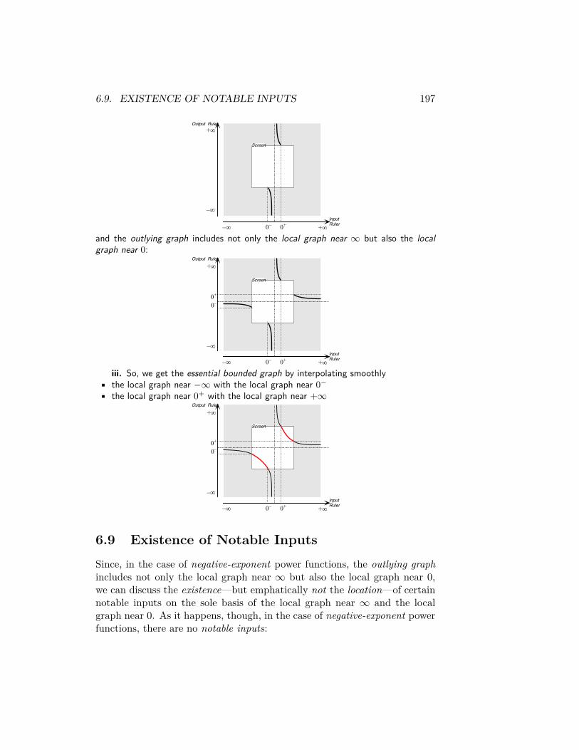
and the outlying graph includes not only the local graph near ∞ but also the localgraph near 0:

Output Ruler

Input Ruler

Screen

+∞–∞ 0– 0+

0–0+

+∞

–∞

iii. So, we get the essential bounded graph by interpolating smoothly• the local graph near −∞ with the local graph near 0−• the local graph near 0+ with the local graph near +∞

Output Ruler

Input Ruler

Screen

+∞–∞ 0– 0+

0–0+

+∞

–∞

6.9 Existence of Notable InputsSince, in the case of negative-exponent power functions, the outlying graphincludes not only the local graph near ∞ but also the local graph near 0,we can discuss the existence—but emphatically not the location—of certainnotable inputs on the sole basis of the local graph near ∞ and the localgraph near 0. As it happens, though, in the case of negative-exponent powerfunctions, there are no notable inputs:


1. Since the features at the transitions are always the same, there is nofeature-sign change input.

EXAMPLE 18. Given the negative-exponent power function whose outlying graph isOutput Ruler

Input Ruler

Screen

+∞–∞

0

+∞

–∞

0

there does not have to be any feature-sign change input:Output Ruler

Input Ruler

Screen

+∞–∞

0

+∞

–∞

0

2. Since 0 is an ∞-height input, there is no 0-feature input.

EXAMPLE 19. Given the negative-exponent power function whose outlying graph isOutput Ruler

Input Ruler

Screen

+∞–∞

0

+∞

–∞

0

there does not have to be any feature-sign change input as shown on the right side and0-feature inputs would require a fluctuation as shown on the left side:

6.10. ESSENTIAL GLOBAL GRAPH 199

Output Ruler

Input Ruler

Screen

+∞–∞

0

+∞

–∞

0

3. Since 0 is an ∞-height input, there is no extremum input.EXAMPLE 20. Given the negative-exponent power function whose outlying graph is

Output Ruler

Input Ruler

Screen

+∞–∞

0

+∞

–∞

0

there does not have to be any extreme input as the only possible one would be 0 beinga minimum input being clipped by too small an extent of the output ruler:

Output Ruler

Input Ruler

Screen

+∞–∞

0

+∞

–∞

0

However, this cannot be the case because, as we saw earlier, nearby inputs get largerand larger outputs.

6.10 Essential Global Graph

We get the essential global graph of a regular positive-exponent power func-tion by assembling all the information we found above, that is:• We draw the local graph near ∞,• We draw the local graph near 0,


• We join smoothly across the screen the local graphs.As with positive-power functions, there are two ways in which we can drawthe essential global graph. We can make:

i. A Mercator drawing in which we draw the global graph on a flatsurface such as a blackboard, a computer screen, or a piece of paper. Thislets the essential bounded graph play a central role and relegates ∞ wherewe cannot see it.

ii. AMagellan drawing in which we draw the global graph on aMagellanscreen, which shows∞ but introduces distortions and is a lot harder to drawas we usually cannot really draw it on a sphere but can only make perspectivedrawings as in this text.A Magellan drawing provides a better insight in what is happening near 0.In particular, we can see better the difference between:• An ∞ height input for an odd negative-power function

EXAMPLE 21. Given the function JUDY whose input-output rule is

xJUDY−−−−−−→ JUDY (x) = (−12.84) · x−3

= −12.84x · x · x︸︷︷︸

3 copies of x

here is the Magellan drawing of the global graph of JUDY :

0-in

put l

evel

0-output level

0+0–

+∞–∞

• An ∞ height input for an even negative-exponent power functions.EXAMPLE 22. Given the function KRIS whose input-output rule is

xKRIS−−−−−−→ KRIS(x) = (+44.08) · x−4

= +44.08x · x · x · x︸︷︷︸4 copies of x

here is the Magellan drawing of the global graph of KRIS:

6.11. TYPES OF GLOBAL GRAPHS 201

0-in

put l

evel

0-output level0+0–

+∞–∞

6.11 Types of Global GraphsEach type of power function has a different qualitative global graph. Hereagain, the qualitative global graph is shown both from “nearby” and from“faraway”.

Input-output rule Essential Graph From “faraway”

xNEP−−−→ NEP (x) = +x−even

Output Ruler

Input Ruler

0

0 +∞–∞

–∞

+∞

Screen

xNEN−−−→ NEN(x) = −x−even

Output Ruler

Input Ruler

0

0 +∞–∞

–∞

+∞

Screen

xNOP−−−→ NOP (x) = +x−odd

Output Ruler

Input Ruler

0

0 +∞–∞

–∞

+∞

Screen



Input-output rule Essential Graph From “faraway”

xNON−−−→ NON(x) = −x−odd

Output Ruler

Input Ruler

0

0 +∞–∞

–∞

+∞

Screen

negative-exponent power functions - free math...

Documents