negative bending moment coefficients for continuous...

JAZAN UNIVERSITY College of Engineering

CIVIl ENgINEERINg DEpARTmENT

NEGATIVE BENDING MOMENT COEFFICIENTS FOR CONTINUOUS BEAMS

By

Team Members:

1. Abdullah Abdulmajeed Atti

2. Mohammed Meghis Al Qhtani

3. Majeed Ali Mahnashi

4. Medwah Iz’zi

5. Anwar Rfa’ai

Supervisor:

Dr. Fathelrahaman Mohamed Adam

A Senior Project Final Report submitted in partial fulfillment of the requirement for

the degree of BACHELOR OF Science (B. Sc.),

in Civil Engineering

(2/1437 h)

‡\Ü]p;Ï¬Ÿ]p

ÔãÑ·7^=ÔÎŸ‘

قسم اهلندسة املدنية

معامالت العزم السالب للعارضات املستمرة

طالب فريق العمل

مشرف املشروع

flÉb=Ñ›®=‚πàÿ^=ykÃ=KÉ

تقر�ر مرشوع التخرج مقدم للحصول �ىل در�ة الباكلوريوس

ىف الهندسة املدنية

)1437صفر/(




APPROVAL RECOMMENDED: Examination Committee:

1. Professor Dr. Hossam Eldin Mohamed Sallam

2. Professor Dr. Ahmed Ahmed El-Abbasy

3. Dr. Ali Eltoum Hassaballa

PROJECT SUPERVISOR Dr. Fathelrahman Mohamed Adam

Date DEPARTMENT HEAD Dr. Mohamed Mubarki

Date COURSE INSTRUCTOR

Date APPROVED DEAN OF COLLEGE OF ENGINEERING

Dr. Jabril Ahmed Khamaj

Date

http://colleges.jazanu.edu.sa/sites/en/eng/Pages/Members/Jabril_Khamaj.aspx�




By

Team Members:

1. Abdullah Abdulmajeed Atti

2. Mohammed Meghis Al Qhtani

3. Majeed Ali Mahnashi

4. Medwah Iz’zi

5. Anwar Rfa’ai

Supervisor:

Dr. Fathelrahaman Mohamed Adam

A Senior Project Final Report submitted in partial fulfillment of the requirement for

the degree of BACHELOR OF Science (B. Sc.),

in

ii

Civil Engineering

(2/1437 h)

ABSTRACT This research presents the results of studies on the negative bending moments in

continuous beams caused by uniformly distributed load exerted over full span

lengths of beam. An elastic analysis based on moment distribution method is

attempted to deduce the coefficients of negative moments for continuous beams

through computing 115 examples with adopting beams of two spans and three

spans and changing their spans lengths. The results are summarized in Tables and

charts for the convenience of practical estimation of these coefficients of bending

moments. The values of the coefficients of negative bending moments can be easily

derived from the charts with a sufficient accuracy emphasized by some numerical

examples carried in this research.

iii

DEDICATION

To my Father, ………………., who, through his financial and moral support was the source of inspiration and the mainstay in my attaining an education, I dedicate this project.

iv

ACKNOWLEDGEMENT This project was written under the direction and supervision of Dr. ……………….. I

would like to express my sincere appreciation to him for the interest and assistance given to me.

v

TABLE OF CONTENTS Page Title Chapter

4 Abstract 5 6 7 7 7 9

1.1 Introduction 1.2Statement of the Problem 1.3Objectives of the Research 1.4Methodology 1.5Outlines of Research Literature Review

CHAPTER ONE General Introduction and

Literature Review

12 13 13 14 15 15

16

3.1 Introduction 3.2 Moment Distribution Method

3.2.1The Fixed End Moments 3.2.2Distribution Factors 3.2.3Carry Over

3.3 Analysis of Continuous Beams 3.3.1 Calculation of Positive Moments Coefficients

CHAPTER TWO Analysis of Continuous

Beams

20 20 20 22 22

4.1 Continuous Beam of Two Spans 4.1.1 Span Lengths 4.1.2 Positive Moment Coefficients

4.2 Continuous Beam of Three Spans 4.2.1 Span Lengths 4.2.2Positive Moment Coefficients

Numerical Example

CHAPTER FOUR Results and Discussion

32

CONCLUSION…………………………… CHAPTER FOUR Conclusions and

Recommendations 33 …………………………………. REFERENCES

vi

LIST OF TABLES

page Title Chapter

18

19

Table (1): Spreadsheet for Calculation of Positive Moments Coefficients for Continuous Beams of Two Spans. Table (2):Spreadsheet for Calculation of Positive Moments Coefficients for Continuous Beams of Three Spans.

Chapter three

20

20

22 23

Table (3): Different Spans Lengths for the

Continuous Beam of Two Spans

Model.

Table (4): Positive Moment Coefficients for the

Beam of Two Spans.

Table (5): Different Spans Lengths for the

Continuous Beam of Three Spans

Model.

Table (6): Positive Moment Coefficients for the

Beam of Three Spans.

Chapter four

vii

LIST OF FIGURES

page Title Chapter

14

14

14

16

16

17

17

Fig. (1)a: Fixed End Moments due to uniformly distributed load in case the ends of the beams are fixed.

Fig. (1)b: Fixed End Moment due to uniformly distributed load in case one end of beam pinned andthe other is fixed. Fig. (2): Two Elements Connected at Joint B Fig. (3): Continuous Beam of two spans where SR2 ranges between 0.6to . Fig. (4): Continuous Beam of three spans where SR2R and SR3R range between 0.6 and 1.5 .

Fig.(5):Shear Force Calculation by Balancing the Forces at the End of the Element .

Fig. (6):Naming of Positive Moments Coefficients for Two and Three spans.

Chapter

three

21

25

26

27

Fig. (7): Positive Moment Coefficients for the Two- Spans Continuous Beam .

Chart 1: Coefficient D1-L for 3-spans, S2 & S3 (0.6-2.0).

Chart 2: Coefficient D2 , for 3-spans, S2 & S3 (0.6-

2.0)

Chart 3: Coefficient D1-R, for 3-spans, S2 & S3 (0.6-2.0).

Chapter

four

1

CHAPTER ONE

GENERAL INTRODUCTION

1.1 General Introduction:

Structural analysis is a very old art and is known to human beings since early

civilizations. The Pyramids constructed by Egyptians around 2000 B.C. stands

today as the testimony to the skills of master builders of that civilization. Many

early civilizations produced great builders, skilled craftsmen who constructed

magnificent buildings such as the Parthenon at Athens (2500 years old), the great

Stupa at Sanchi (2000 years old), TajMahal (350 years old), Eiffel Tower (120

years old) and many more buildings around the world. These monuments tell us

about the great feats accomplished by these craftsmen in analysis, design and

construction of large structures. Today we see around us countless houses, bridges,

fly-overs, high-rise buildings and spacious shopping malls. Planning, analysis and

construction of these buildings is a science by itself.

Structural analysis is the prediction of the performance of a given structure under

prescribed loads and/or other external effects, such as support movements and

temperature changes. The performance characteristics commonly of interest in the

design of structures are stresses or stress resultants, such as axial forces, shear

forces, and bending moments; deflections; and support reactions. Thus, the analysis

of a structure usually involves determination of these quantities as caused by a

given loading condition.

Structures can be classified into five basic categories, namely, tension structures

(e.g., cables and hangers), compression structures (e.g., columns and arches),

trusses, shear structures (e.g., shear walls), and bending structures (e.g., beams and

rigid frames).

2

There are many methods of structural analysis include analytical methods which

depend on using manual calculation and also include numerical methods which

most of them used computers. In addition to existence of wide spreading of

engineering software used in structural analysis. In spite of talking mentioned, there

is needing of using simplified and quick methods instead of using more

calculations or needing for using software in some practice.

A continuous beam is a structural component which is classified as a statically

indeterminate multispan beam on hinged supports along its length. These are

usually in the same horizontal plane, and the spans between the supports are in one

straight line. The end spans may be cantilever, may be freely supported or fixed

supported. The continuous beam provides resistance to bending when a load is

applied. At least one of the supports of a continuous beam must be able to develop

a reaction along the beam axis. Continuous beams are used in structural designs

when three or more spans exist. Continuous beams occur frequently in cast in situ

construction when a single span of construction is linked to an adjoining span also

commonly used in bridges. Bending moment of continuous beams does not confine

to a single span only but it will affect the whole system. The continuous beam is

much stiffer and stronger than the simply supported beam because the continuity

tends to reduce the maximum moment on a beam and makes it stiffer. To design

any structure which a continuous beam is a part of it, it is necessary to know the

bending moments and shearing forces in each member.

Various methods have been developed for determining the bending moments and

shearing force oncontinuous beams, these methods are interrelated to each other to

a greater or lesser extent. Most of the well-known individual methods of structural

analysis such as the theorem of three moments which it proposed by Clapeyron (is

French engineer and physicist), slope deflection, fixed and characteristic points,

and moment distribution methods. These approaches generally lends their self

3

better to hand computation than numerical methods such as flexibly methods,

stiffness method or finite element method. To avoid the need to solve large sets of

simultaneous equations, such as are required with the three-moment theorem or

slope deflection, methods involving successive approximations have been devised,

such as hardy cross moment distribution.

A coefficient method is used for the analysis of continuous as approximate method

by most of codes of practice such as ACI code, BS8110, EC and SBC. The

approximate method allows for various load patterns also allows for the real

rotation restraint at external supports, where the real moment is not equal to zero.

Elastic analysis gives systematic zero moment values at all external pin supports.

The coefficient method is thus more realistic but is only valid for standard cases. It

is advised to use this method whenever its conditions of application are satisfied.

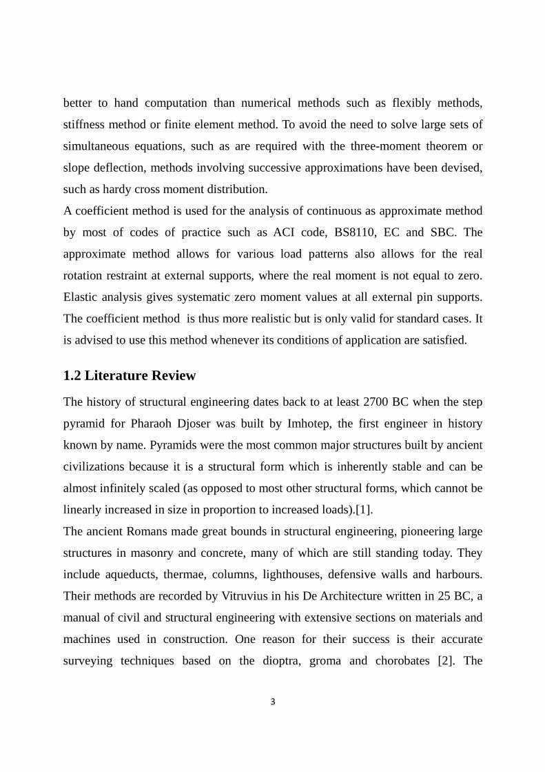
1.2 Literature Review

The history of structural engineering dates back to at least 2700 BC when the step

pyramid for Pharaoh Djoser was built by Imhotep, the first engineer in history

known by name. Pyramids were the most common major structures built by ancient

civilizations because it is a structural form which is inherently stable and can be

almost infinitely scaled (as opposed to most other structural forms, which cannot be

linearly increased in size in proportion to increased loads).[1].

The ancient Romans made great bounds in structural engineering, pioneering large

structures in masonry and concrete, many of which are still standing today. They

include aqueducts, thermae, columns, lighthouses, defensive walls and harbours.

Their methods are recorded by Vitruvius in his De Architecture written in 25 BC, a

manual of civil and structural engineering with extensive sections on materials and

machines used in construction. One reason for their success is their accurate

surveying techniques based on the dioptra, groma and chorobates [2]. The

4

foundations of modern structural engineering were laid in the 17th century by

Galileo Galilei, Robert Hooke and Isaac Newton with the publication of three great

scientific works.

Structural engineering has long been a part of human endeavor, but Galileo is

considered to be the originator of the theory of structures [3]. Following his

pioneering work, many other people have made significant contributions. The

availability of computers has revolutionized structural analysis.

Among the important investigators and accomplishments were: James Clerk

Maxwell (1831-1879) of Scotland, for the Reciprocal Deflection theorem in 1864;

Otto Mohr (1835-1918) of Germany for Elastic Weights in 1870; Alberto

Castigliano of Italy for Least Work theorem in 1873; Charles E. Green of the

United States for the Moment-Area theorems in 1873; B.P.E Clapeyron of France

for the Three-Moment theorem in 1857. In the United States of America two great

developments in Statistically Indeterminate Structure Analysis were made by

GEORGE A. MANEY (1888-1947) and HARDY CROSS (1885-1959). GEORGE

A. MANEY introduced Slope Deflection method in 1915 at University of

Minnesota engineering publication. In Germany, BENDIXEN introduced Slope

Deflection in 1914. For nearly 15 years, until the introduction of Moment

Distribution, Slope Deflection was the popular method used for the Analysis of

continuous beams and frames in the United States of America. [4]. Another most

common approximate method of analyzing building frames for LATERAL LOADS

such as winds, earthquake (seismic) is the PORTAL method which was presented

by Albert Smith in the Journal of the Western Society of Engineers in 1915.

Another simple method of analyzing building frames for Lateral Loads is the

Cantilever method presented by A.C. Wilson in engineering record, 1908. These

methods are said to be satisfactory for buildings with height not in excess of 25 to

35 stories.

5

Structural engineering theory was again advanced in 1930 when Professor Hardy

Cross developed his Moment distribution method, allowing the real stresses of

many complex structures to be approximated quickly and accurate [5].

A coefficient method is used for the analysis of continuous as approximate method

by most of codes of practice such as ACI Code [6], BS8110 [7], EC2 [8] and more.

The codes give the coefficients of bending moments and shear force under some

provisions for continuous beams and slabs. As an example the ACI code provisions

require two or more continuous spans, spans of equal length or having the larger of

two adjacent spans not being greater than the shorter by more than 20 percent,

loads being uniformly distributed, unfactored live load not exceeding three times

unfactored dead load, and the members being prismatic.

Comprehensive work was done by Reynolds and Steedman [9] to calculate bending

moments, shear forces and deflections for simple and continuous beams under

different conditions of loading and supports and that by using Equations and/or

Charts and Tables.

A shear and moment formulas with diagrams for simply supported beams and

continuous beams of two spans were done by American Wood Council [10].

Khuda and Anwar [11] were studying the behaviour of beams and developed

moment coefficients for beams of different spans and varying span ratio.

Fathelrahman, Hassaballa and Sallam[12] deduced negative moment coefficients

for continuous beams of equal and unequal spans.

Fathelrahman [13], derive coefficients for the negative and positive moments for

continuous beams of two, three and four spans of different spans lengths and

produce multiple charts for these coefficients.

This research derive and generates charts for coefficients of negative bending

moments for continuous beams of 2-spans and 3-spans of different spans lengths

controlled by spans ratio depending on the fist span and ranging between 0.6 to 2.0

6

for the two spans and between 0.6 to 1.5 for the three spans. The ratios are

calculated by dividing all spans by the length of the first span. The study was

carried under assumptions that the beams are full spans loaded by uniformly

distributed load and the cross sections are prismatic. The analysis was done

according to the moment distribution method. With changing the ratio of spans, a

number of 15 examples for two spans were obtained, while for three spans 100

examples were obtained.

1.3 Statement of the Problem:

Even with the availability of computers, most engineers find it desirable to make a

rough check of results, using approximate means, to detect gross errors. Further, for

structures of minor importance, it is often satisfactory to design on the basis of

results obtained by rough calculation. For these reasons, many engineers at some

stage in the design process estimate the values of moments, shears, and thrusts at

critical locations, using approximate sketches of the structure deflected by its loads.

This research help in easing the process of calculating the bending moment without

difficulties and without more calculation by deriving coefficients for calculating

negative moments for continuous beams consisting of two and three spans.

1.4 Objectives of the Research:

This research aim to the following objectives:

1. To analyze continuous beams consisting of two and three spans with

different spans lengths.

2. To derive coefficients of negative bending moment for the continuous beams

of two and three spans with different spans lengths.

3. To draw a charts for the coefficients of negative bending moments.

4. To deduce equations for the negative moments coefficients.

7

1.5 Methodology:

To achieve the objectives mentioned above, the following steps must be followed:

1. Using the method of moment distribution to do an elastic analysis of

continuous beams of two and three spans.

2. Using spreadsheets to derive the coefficients of negative moment according

to the results of analysis.

3. Using Origin Software to plot charts for the coefficients of negative moments

for two and three spans.

4. Using Curvexpert Software to deduce equations to calculate the coefficients

of negative moments.

1.6 Outlines of Research:

This research contains five Chapters as explained in the following:

• Chapter One contains general introduction about the analysis of structures

and literature review.

• Chapter Two describes the general procedure of analyzing continuous

beams by using moment distribution and deriving the necessary equations

for calculating bending moments and after that deducing the coefficients.

• Chapter Three explain the results of the analysis graphically

• Chapter Four discuss the results of the numerical examples.

• Chapter Five contains the conclusions and some recommendations.

8

CHAPTER TWO

ANALYSIS OF CONTINUOUS BEAMS

2.1 Introduction:

A beam is a horizontal structural element that is capable of withstanding load

primarily by resisting bending, bending moments are the bending forces induced to

the material as a results of external loads and due to its own weight over the span. A

Continuous beam is a beam that is supported by more than two supports and it is

statistically indeterminate structure and is known as Redundant or Indeterminate

Structure as they cannot be analysed by making use of basic equilibrium.

The continuous beams have some advantages which have more vertical load

capacity this means they can support a very heavy loads and the deflection at the

middle of the span is minimal as opposed to simple supported beams. The main

disadvantages of continuous beams is that there is a difficulty in the analysis and in

the design of it.

Various methods have been developed for determining the bending moments and

shearing force on continuous beams. These methods are interrelated to each other

to a greater or lesser extent. Most of the well-known individual methods of

structural analysis such as the theorem of three moments, slope deflection, fixed

and characteristic points, and moment distribution and characteristic points , and

moment distribution and its variants, are stiffness methods: this approach generally

lends itself better to hand computation than do flexibly methods . to avoid the need

to solve large sets of simultaneous equations, such as are required with the three-

moment theorem or slope deflection, methods involving successive approximations

have been devised, such as hardy cross moment distribution and south well's

relaxation method [9].

9

Perhaps the system best known at present for analysing continuous beams by hand

is that of moment distribution, devised by Hardy cross. The method, which derives

from slop-deflection principles, avoids the need to solve sets of simultaneous

equations directly by employing instead a system of successive approximation

which may be terminated as soon as the required degree accuracy has been reached.

One particular advantage of this is that it is often clear, even after only one

distribution cycle, whether or not the final values will be acceptable. If not, the

analysis need not be continued further, thus saving much unnecessary work. The

method is simple to remember and apply and the step-by-step procedure. Hardy

cross moment distribution is described in detail in most textbooks dealing with

structural analysis.

2.2 Moment Distribution Method:

The method as mentioned before was invented by Professor Hardy Cross of

University of Illinois of U.S.A. The method can be used to analyze all types of

statically indeterminate beams or rigid frames. Essentially it consists in solving the

linear simultaneous equations that were obtained in the slope-deflection method by

successive approximations or moment distribution. Increased number of cycles

would result in more accuracy.

The moment distribution method starts with assuming that each joint in the

structure is fixed, then joints are “unlocked” and “locked” in succession until each

joint has rotated to its final position. During this process, internal moments at the

joints are “distributed” and balanced. The resulting series can be terminated

whenever one reaches the degree of accuracy required. After member end moments

are obtained, all member stress resultants can be obtained from the laws of statics.

For the next three decades, moment distribution provided the standard means in

engineering offices for the analysis of indeterminate beams and frames. Even now,

10

it serves as the basic analytical tool for analysis if computer facilities are not

available.

The moment distribution method involves the following steps:

1. Determination of fixed end moments due to externally applied loads for all

the members.

2. Determination of distribution factors for members meeting at each joint.

3. The sum of the fixed end moments at each joint is calculated (unbalanced

moment). Next calculate the balancing moments which is equal in magnitude

but opposite in sign to this sum.

4. At each joint distribution of balancing moments to each member in the ratios

of distribution factors.

5. Carry over half the distributed moments to the other end of each member.

6. Repeat the cycle (4) and (5) once it is completed for all the joints of the

structure.

This process continues till sufficient accuracy of results is achieved with attention

to that the process should stop only after a distribution and never after a carry over.

2.2.1 The Fixed End Moments:

The fixed end moments are reaction moments developed in abeam member under

certain load conditions with both ends fixed against rotation. A beam with both

ends fixed is statically indeterminate to the 3rd degree, and any structural analysis

method applicable on statically indeterminate beams can be used to calculate the

fixed end moments.

In this research we introduce only distributed load full spans for each member, the

fixed end moments can be calculated from the formulas shown in Fig. (2.1)a and

(2.1)b. As sign convention, the clockwise moment consider as negative and counter

clockwise moment consider as negative.

11

Fig. (2.1)a: Fixed End Moments due to uniformly distributed load in case the ends

of the beams are fixed

Fig. (2.1)b: Fixed End Moment due to uniformly distributed load in case one end of

beam pinned and the other is fixed. 2.2.2 Distribution Factors:

Is the factor calculated for each element that connected at a given joint and

multiplied bythe moment at this joint to give the distributed moment to each

element. As an example if there are two elements AB and BC connected at joint B

which have outbalance moment (M) and this moment must be distributed to each

element. The distribution mainly depends on the material property (E, Elastic

Modulus) and geometric data (L, span length and I, second moment of inertia) for

each element as illustrated in Fig. (2.2).

Fig. (2.2): Two Elements Connected at Joint B Mathematically the distribution factors need to distribute the moment (M) to the

two elements can be calculated by using the following formula:

�� =��

��, �� =

��

��(2.1)

M

A

C

B

Deflected Shape �� = 0

�� = 0

�� =?

EA, IA,

EB, IB,

w ��

8

l

w

l

��

12

��

12

12

Where k is the stiffness which defined by the moment at one end of a member

necessary to produce unit rotation of that end when the other end is held fixed. It

iscalculated by using the elements properties as:

�� =4��

��, �� =

4��

��, �� = �� + �� (2.2)

The distribution factor is calculated for each joint so each element hastwo

distributions factors at its two ends.

2.2.3 Carry Over:

Is the ratio of the moment at the end to the moment producing rotation at the

rotating end. It can be derived using slope-deflection equations and numerically is

equal to ½.

2.3 Analysis of Continuous Beams:

The continuous beam consisting of two and three spans were analysed according to

the moment distribution method by following the general steps of the procedure.

These steps are implemented in the spreadsheets in Excel file under the following

assumption:

1. The beam of the same material and the cross sections of the beam are

prismatic (EI = constant).

2. All the supports are hinges.

3. The loads applied is uniformly distributed load full span and have a unit

value through out (w=1.0 kN/m).

4. The span lengths are controlled by the spans ratio (S), which all spans were

divided by the first span length (L1) this gives S1 = 1.0.

Fig. (2.3) illustrate some assumptions for beam of two spans, and Fig. (2.4)

illustrate some assumption for beam of three spans.

13

Fig. (2.3): Continuous Beam of two spans where S2 ranges between 0.6 to 2.0

Fig. (2.4): Continuous Beam of three spans where S2 and S3 range between 0.6 and

1.5

2.3.1 Calculation of Negative Moments Coefficients:

With following steps of moment distribution method the negative moments at

supports have been calculated with aid of using spreadsheets. The coefficients of

moments can be calculated by dividing the support moments by the span length.

Since the support moment is in between two spans at left and at right, an average of

these spans is used to calculate the coefficient of moment. Later the same average

is used to calculate the bending moment once the coefficient being derived from

chart. Accordingly the coefficient C can be calculated using Equation (2.3).

� =��

�½(� + �!)"�(2.3)

where:

C is the negative moment coefficient at the internal supports (with taken

w=1.0).

Ms is the negative moment at support.

LL is the length if span to left of support

LR is the span length right to the support.

The negative moments coefficients for the two and three spans are coded as shown

in Fig. (2.5).

w = 1 kN/m

S2= L2/L1 S1=L1/L1=1 S3= L2/L1

S1=L1/L1=1 S2= L2/L1

w = 1 kN/m

14

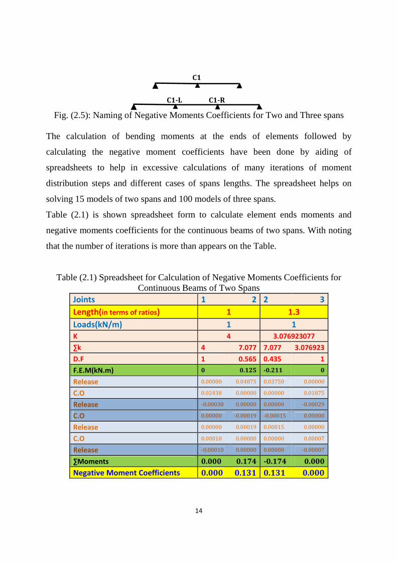
Fig. (2.5): Naming of Negative Moments Coefficients for Two and Three spans

The calculation of bending moments at the ends of elements followed by

calculating the negative moment coefficients have been done by aiding of

spreadsheets to help in excessive calculations of many iterations of moment

distribution steps and different cases of spans lengths. The spreadsheet helps on

solving 15 models of two spans and 100 models of three spans.

Table (2.1) is shown spreadsheet form to calculate element ends moments and

negative moments coefficients for the continuous beams of two spans. With noting

that the number of iterations is more than appears on the Table.

Table (2.1) Spreadsheet for Calculation of Negative Moments Coefficients for Continuous Beams of Two Spans

Joints 1 2 2 3

Length(in terms of ratios) 1 1.3

Loads(kN/m) 1 1

K 4 3.076923077

∑k 4 7.077 7.077 3.076923

D.F 1 0.565 0.435 1

F.E.M(kN.m) 0 0.125 -0.211 0

Release 0.00000 0.04875 0.03750 0.00000

C.O 0.02438 0.00000 0.00000 0.01875

Release -0.00038 0.00000 0.00000 -0.00029

C.O 0.00000 -0.00019 -0.00015 0.00000

Release 0.00000 0.00019 0.00015 0.00000

C.O 0.00010 0.00000 0.00000 0.00007

Release -0.00010 0.00000 0.00000 -0.00007

∑Moments 0.000 0.174 -0.174 0.000

Negative Moment Coefficients 0.000 0.131 0.131 0.000

C1-R C1-L

C1

15

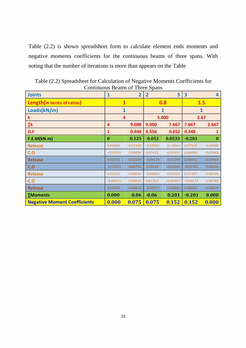
Table (2.2) is shown spreadsheet form to calculate element ends moments and

negative moments coefficients for the continuous beams of three spans. With

noting that the number of iterations is more than appears on the Table

Table (2.2) Spreadsheet for Calculation of Negative Moments Coefficients for

Continuous Beams of Three Spans

Joints 1 2 2 3 3 4

Length(in terms of ratios) 1 0.8 1.5

Loads(kN/m) 1 1 1

k 4 5.000 2.67

∑k 4 9.000 9.000 7.667 7.667 2.667

D.F 1 0.444 0.556 0.652 0.348 1

F.E.M(kN.m) 0 0.125 -0.053 0.0533 -0.281 0

Release 0.00000 -0.03185 -0.03981 0.14864 0.07928 0.00000

C.O -0.01593 0.00000 0.07432 -0.01991 0.00000 0.03964

Release 0.01593 -0.03303 -0.04129 0.01298 0.00692 -0.03964

C.O -0.01652 0.00796 0.00649 -0.02064 -0.01982 0.00346

Release 0.01652 -0.00642 -0.00803 0.02639 0.01407 -0.00346

C.O -0.00321 0.00826 0.01319 -0.00402 -0.00173 0.00704

Release 0.00005 -0.00015 -0.00019 0.00006 0.00003 -0.00010

∑Moments 0.000 0.06 -0.06 0.201 -0.201 0.000

Negative Moment Coefficients 0.000 0.075 0.075 0.152 0.152 0.000

16

CHAPTER THREE

DERIVATION OF NEGATIVE BENDING MOMENT COEFFICIENTS

3.1 Continuous Beam of Two Spans 3.1.1 Span Lengths:

With referring to Figure (2.3), 15 models of continuous beams of two spanswere gained by changing the span lengths according to the values shown in Table (3.1).

Table (3.1): Different Spans Lengths for the Continuous Beam of Two Spans Model

S1 1 1 1 1 1 1 1 1 1 1 1 1 1 1 1

S2 0.6 0.7 0.8 0.9 1 1.1 1.2 1.3 1.4 1.5 1.6 1.7 1.8 1.9 2

S1 = L1/L1, S2 = L2/L1 3.1.2Negative Moment Coefficients Results: According to the span lengths illustrated in Table (3.1) and by using spreadsheet

form shown in Table (2.1), the results obtained for the negative moment

coefficients are listed in the Tables (3.2)

Table (3.2): Negative Moment Coefficients for the Beam of Two Spans

S1 S2 C1

1 0.6 0.148

1 0.7 0.137

1 0.8 0.130

1 0.9 0.126

1 1 0.125

1 1.1 0.126

1 1.2 0.128

1 1.3 0.131

1 1.4 0.135

1 1.5 0.14

1 1.6 0.145

1 1.7 0.15

1 1.8 0.156

1 1.9 0.161

1 2 0.167

17

The values of negative moments coefficients shown in Table (3.2), were plotted as

shown in Figure (3.1).

Fig. (3.1): Negative Moment Coefficients for the Two-Spans Continuous Beam

Instead of using the coefficients listed in Table (3.2) or using the Graph shown in Fig. (3.1), We can use equation for the coefficient (C1). This equation is derived by using CurveExpert 1.3 software which it find the best curve through fitting the data by adopting malty models and the best equation gained for the coefficients is the polynomial equation shown in Equation (3.1). The accuracy of these equations are measured by standard deviation of 0.001 and coefficient of correlation equal to 0.998.

�1 = 0.28208 − 0.35810(&2) + 0.25232(&2)� − 0.05119(&2)((3.1)

18

3.2 Continuous Beam of Three Spans

3.2.1 Span Lengths:

With referring to Figure (2.4), 100 models of continuous beams of three spans were gained by changing the span lengths according to the values shown in Tables form Table (3.3)a to Table (3.3)j . with notice that S1 = 1, S2 = L2/L1, S3 = L2/L1.

Table (3.3)a: Spans Lengths for Beam of Three Spans Model (S2 = 0.6) S1 1.0 1.0 1.0 1.0 1.0 1.0 1.0 1.0 1.0 1.0 S2 0.6 0.6 0.6 0.6 0.6 0.6 0.6 0.6 0.6 0.6 S3 0.6 0.7 0.8 0.9 1.0 1.1 1.2 1.3 1.4 1.5

Table (3.3)b: Spans Lengths for Beam of Three Spans Model (S2 = 0.7)

S1 1.0 1.0 1.0 1.0 1.0 1.0 1.0 1.0 1.0 1.0 S2 0.7 0.7 0.7 0.7 0.7 0.7 0.7 0.7 0.7 0.7 S3 0.6 0.7 0.8 0.9 1.0 1.1 1.2 1.3 1.4 1.5

Table (3.3)c: Spans Lengths for Beam of Three Spans Model (S2 = 0.8)

S1 1.0 1.0 1.0 1.0 1.0 1.0 1.0 1.0 1.0 1.0 S2 0.8 0.8 0.8 0.8 0.8 0.8 0.8 0.8 0.8 0.8 S3 0.6 0.7 0.8 0.9 1.0 1.1 1.2 1.3 1.4 1.5

Table (3.3)d: Spans Lengths for Beam of Three Spans Model (S2 = 0.9)

S1 1.0 1.0 1.0 1.0 1.0 1.0 1.0 1.0 1.0 1.0 S2 0.9 0.9 0.9 0.9 0.9 0.9 0.9 0.9 0.9 0.9 S3 0.6 0.7 0.8 0.9 1.0 1.1 1.2 1.3 1.4 1.5

Table (3.3)e: Spans Lengths for Beam of Three Spans Model (S2 = 1.0)

S1 1.0 1.0 1.0 1.0 1.0 1.0 1.0 1.0 1.0 1.0 S2 1.0 1.0 1.0 1.0 1.0 1.0 1.0 1.0 1.0 1.0 S3 0.6 0.7 0.8 0.9 1.0 1.1 1.2 1.3 1.4 1.5

Table (3.3)f: Spans Lengths for Beam of Three Spans Model (S2 = 1.1)

S1 1.0 1.0 1.0 1.0 1.0 1.0 1.0 1.0 1.0 1.0 S2 1.1 1.1 1.1 1.1 1.1 1.1 1.1 1.1 1.1 1.1 S3 0.6 0.7 0.8 0.9 1.0 1.1 1.2 1.3 1.4 1.5

Table (3.3)g: Spans Lengths for Beam of Three Spans Model (S2 = 1.2)

S1 1.0 1.0 1.0 1.0 1.0 1.0 1.0 1.0 1.0 1.0 S2 1.2 1.2 1.2 1.2 1.2 1.2 1.2 1.2 1.2 1.2 S3 0.6 0.7 0.8 0.9 1.0 1.1 1.2 1.3 1.4 1.5

19

Table (3.3)h: Spans Lengths for Beam of Three Spans Model (S2 = 1.3) S1 1.0 1.0 1.0 1.0 1.0 1.0 1.0 1.0 1.0 1.0 S2 1.3 1.3 1.3 1.3 1.3 1.3 1.3 1.3 1.3 1.3 S3 0.6 0.7 0.8 0.9 1.0 1.1 1.2 1.3 1.4 1.5

Table (3.3)i: Spans Lengths for Beam of Three Spans Model (S2 = 1.4)

S1 1.0 1.0 1.0 1.0 1.0 1.0 1.0 1.0 1.0 1.0 S2 1.4 1.4 1.4 1.4 1.4 1.4 1.4 1.4 1.4 1.4 S3 0.6 0.7 0.8 0.9 1.0 1.1 1.2 1.3 1.4 1.5

Table (3.3)j: Spans Lengths for Beam of Three Spans Model (S2 = 1.5)

S1 1.0 1.0 1.0 1.0 1.0 1.0 1.0 1.0 1.0 1.0 S2 1.5 1.5 1.5 1.5 1.5 1.5 1.5 1.5 1.5 1.5 S3 0.6 0.7 0.8 0.9 1.0 1.1 1.2 1.3 1.4 1.5

3.2.2 Negative Moment Coefficients Results for Beam of Three Spans :

According to the span lengths illustrated in Tables (3.3)a-j and by using spreadsheet form shown in Table (2.2), the results obtained for the negative moment coefficients are listed in the Tables (3.4)a-j

Table (3.4)a: Negative Moment Coefficients for Beam of Three Spans (S2 = 0.6) S1 1.0 1.0 1.0 1.0 1.0 1.0 1.0 1.0 1.0 1.0

S2 0.6 0.6 0.6 0.6 0.6 0.6 0.6 0.6 0.6 0.6

S3 0.6 0.7 0.8 0.9 1.0 1.1 1.2 1.3 1.4 1.5

C1-L 0.144 0.142 0.138 0.135 0.130 0.125 0.119 0.112 0.105 0.097

C1-R 0.062 0.079 0.095 0.110 0.125 0.139 0.152 0.164 0.176 0.187

Table (3.4)b: Negative Moment Coefficients for Beam of Three Spans (S2 = 0.7)

S1 1.0 1.0 1.0 1.0 1.0 1.0 1.0 1.0 1.0 1.0

S2 0.7 0.7 0.7 0.7 0.7 0.7 0.7 0.7 0.7 0.7

S3 0.6 0.7 0.8 0.9 1.0 1.1 1.2 1.3 1.4 1.5

C1-L 0.128 0.126 0.122 0.118 0.113 0.108 0.102 0.095 0.087 0.079

C1-R 0.068 0.079 0.090 0.102 0.113 0.125 0.136 0.147 0.157 0.167

Table (3.4)c: Negative Moment Coefficients for Beam of Three Spans (S2 = 0.8)

S1 1.0 1.0 1.0 1.0 1.0 1.0 1.0 1.0 1.0 1.0

S2 0.8 0.8 0.8 0.8 0.8 0.8 0.8 0.8 0.8 0.8

S3 0.6 0.7 0.8 0.9 1.0 1.1 1.2 1.3 1.4 1.5

C1-L 0.119 0.117 0.114 0.110 0.106 0.101 0.095 0.089 0.082 0.075

C1-R 0.076 0.082 0.089 0.097 0.106 0.115 0.125 0.134 0.143 0.152

20

Table (3.4)d: Negative Moment Coefficients for Beam of Three Spans (S2 = 0.9) S1 1.0 1.0 1.0 1.0 1.0 1.0 1.0 1.0 1.0 1.0 S2 0.9 0.9 0.9 0.9 0.9 0.9 0.9 0.9 0.9 0.9 S3 0.6 0.7 0.8 0.9 1.0 1.1 1.2 1.3 1.4 1.5

C1-L 0.113 0.111 0.109 0.106 0.102 0.097 0.092 0.087 0.080 0.073

C1-R 0.085 0.087 0.090 0.096 0.102 0.109 0.116 0.124 0.132 0.140

Table (3.4)e: Negative Moment Coefficients for Beam of Three Spans (S2 = 1.0)

S1 1.0 1.0 1.0 1.0 1.0 1.0 1.0 1.0 1.0 1.0 S2 1.0 1.0 1.0 1.0 1.0 1.0 1.0 1.0 1.0 1.0 S3 0.6 0.7 0.8 0.9 1.0 1.1 1.2 1.3 1.4 1.5

C1-L 0.110 0.108 0.106 0.103 0.100 0.096 0.091 0.086 0.080 0.074

C1-R 0.095 0.093 0.093 0.096 0.100 0.105 0.111 0.117 0.124 0.131

Table (3.4)f: Negative Moment Coefficients for Beam of Three Spans (S2 = 1.1)

S1 1.0 1.0 1.0 1.0 1.0 1.0 1.0 1.0 1.0 1.0 S2 1.1 1.1 1.1 1.1 1.1 1.1 1.1 1.1 1.1 1.1 S3 0.6 0.7 0.8 0.9 1.0 1.1 1.2 1.3 1.4 1.5

C1-L 0.108 0.107 0.105 0.103 0.100 0.096 0.092 0.087 0.082 0.076

C1-R 0.104 0.099 0.097 0.098 0.100 0.103 0.107 0.112 0.118 0.123

Table (3.4)g: Negative Moment Coefficients for Beam of Three Spans (S2 = 1.2)

S1 1.0 1.0 1.0 1.0 1.0 1.0 1.0 1.0 1.0 1.0 S2 1.2 1.2 1.2 1.2 1.2 1.2 1.2 1.2 1.2 1.2 S3 0.6 0.7 0.8 0.9 1.0 1.1 1.2 1.3 1.4 1.5

C1-L 0.107 0.107 0.105 0.103 0.101 0.098 0.094 0.090 0.085 0.080

C1-R 0.113 0.106 0.102 0.100 0.101 0.102 0.105 0.109 0.113 0.118

Table (3.4)h: Negative Moment Coefficients for Beam of Three Spans (S2 = 1.3)

S1 1.0 1.0 1.0 1.0 1.0 1.0 1.0 1.0 1.0 1.0 S2 1.3 1.3 1.3 1.3 1.3 1.3 1.3 1.3 1.3 1.3 S3 0.6 0.7 0.8 0.9 1.0 1.1 1.2 1.3 1.4 1.5

C1-L 0.108 0.107 0.106 0.105 0.102 0.100 0.097 0.093 0.089 0.084

C1-R 0.122 0.113 0.107 0.104 0.102 0.103 0.104 0.107 0.110 0.114

Table (3.4)i: Negative Moment Coefficients for Beam of Three Spans (S2 = 1.4)

S1 1.0 1.0 1.0 1.0 1.0 1.0 1.0 1.0 1.0 1.0 S2 1.4 1.4 1.4 1.4 1.4 1.4 1.4 1.4 1.4 1.4 S3 0.6 0.7 0.8 0.9 1.0 1.1 1.2 1.3 1.4 1.5

C1-L 0.109 0.109 0.108 0.107 0.105 0.103 0.100 0.096 0.093 0.088

C1-R 0.130 0.119 0.112 0.107 0.105 0.104 0.104 0.106 0.108 0.111

21

Table (3.4)j: Negative Moment Coefficients for Beam of Three Spans (S2 = 1.5) S1 1.0 1.0 1.0 1.0 1.0 1.0 1.0 1.0 1.0 1.0 S2 1.5 1.5 1.5 1.5 1.5 1.5 1.5 1.5 1.5 1.5 S3 0.6 0.7 0.8 0.9 1.0 1.1 1.2 1.3 1.4 1.5

C1-L 0.111 0.111 0.110 0.109 0.108 0.106 0.103 0.100 0.097 0.093

C1-R 0.138 0.126 0.117 0.111 0.108 0.106 0.105 0.105 0.107 0.109

The values of negative moments coefficients shown in Tables (3.3)a-j, were plotted as shown in Figures (3.2 and 3.3).

Fig. (3.2): Negative Moment Coefficient for the First Left Inner Support of the

Three-Spans Continuous Beam

22

Fig. (3.3): Negative Moment Coefficient for the First Right Inner Support of the

Three-Spans Continuous Beam

23

CHAPTER FOUR

VERIFICATION OF NEGATIVE MOMENT COEFFICIENTS BY USING NUMERICAL EXAMPLES

4.1 Calculation of Bending Moments using Coefficients:

After the coefficients of negative bending moment are obtained the bending

moment for each support can be calculated from the following equation.

M = C w L2 (4.1)

Where:

C is the negative bending moment coefficient.

w is the uniformly distributed load.

L is the average of the two spans lengths besides the coefficient C.

4.2 Verification of Negative Bending Moment Coefficients:

In the following there are seven examples of continuous beams of different spans

lengths, four of two spans and three of three spans, these examples were selected in

order to verify the values of negative moment coefficients that derived and

explained in Chapter Three.

4.2.1 Example 1:

This example consisting of two spans and carries a uniformly distributed load of 12

kN/m through all spans as shown in Fig. (4.1). According to the value of S2

calculated from the spans lengths, the coefficients of negative bending moment for

the internal support was obtained form Table (3.2) and form the Chart of Fig. (3.1)

and also calculated from equation (3.1). The bending moments for the inner support

was calculated using equation (4.1). These moments were compared by one

24

obtained by using PROKON Software Program to check the accuracy and the

difference percentages are calculated and all values were listed in Table (4.1)

Fig. (4.1): Continuous Beam of Example 1

Table (4.1) Calculations of Example 1

Span AB Span BC L(m) 4.0 4.0

S 1 1

Coefficient Support B (C1)

Table 0.125

Chart 0.125

Equation 0.125

Moment by using Coefficients (kN.m) 24

Moment by using PROKON (kN.m) 24

Dif% 0.00%

4.2.2 Example 2:










w = 10 kN/m

4 m

B C

EI=const

4.2 m

A

w = 12 kN/m

4 m

B C

EI=const

4 m

A

25



S 1 1.05


Table 0.125

Chart 0.126

Equation 0.125

Moment by using Coefficients (kN.m) 21.013

Moment by using PROKON (kN.m) 21.05

Dif% 0.38%

4.2.3 Example 3:





and also calculated from equations (3.1) and (3.2). the bending moments for the

inner support was calculated using equation (4.1). These moments were compared

by one obtained by using PROKON Software Program to check the accuracy and

the difference percentages are calculated and all values were listed in Table (4.3)


w = 15 kN/m

4.8 m

B C

EI=const

4 m

A

26

Table (4.3) Calculations of Example 3 Span AB Span BC

L(m) 4.8 4.0

S 1 0.83


Table 0.130

Chart 0.129

Equation 0.128


Moment by using PROKON (kN.m) 37.200

Dif% 0.69%

4.2.4 Example 4:










w = 20 kN/m

4 m

B C

EI=const

8 m

A

27



S 1 2


Table 0.167

Chart 0.167

Equation 0.166


Moment by using PROKON (kN.m) 120

Dif% 0.2%

4.2.5 Example 5:

This example consisting of three spans and carries a uniformly distributed load of

18 kN/m through all spans as shown in Fig. (4.5). According to the value of S2 and

S3 calculated from the spans lengths, the coefficients of negative bending moment

for the two internal supports were obtained form Table (3.4)e and form the Charts

of Figs. (3.2) and (3.3). The bending moments for the two internal supports were

calculated using equation (4.1). These moments were compared by one obtained by

using PROKON Software Program to check the accuracy and the difference

percentages are calculated and all values were listed in Table (4.5).


w = 18 kN/m

4 m B C EI=const

4 m

A

4 m

D

28


Span AB Span BC Span CD L(m) 4.0 4.0 4.0

S 1 1 1

Coefficients Support B

(C1-L)

Support C

(C1-R)

Table 0.1 0.1

Chart 0.1 0.1

Moment by using Coefficients (kN.m) 28.8 28.8

Moment by using PROKON (kN.m) 28.8 28.8

Dif% 0.00% 0.00%

4.2.6 Example 6:




for the internal supports were obtained form Table (3.4)j and form the Charts of

Figs. (3.2) and (3.3). The bending moments for the two internal supports were

calculated using equation (4.1). These moments were compared by one obtained by

using PROKON Software Program to check the accuracy and the difference

percentages are calculated and all values were listed in Table (4.6).


w = 11 kN/m

4 m B C EI=const

6 m

A

5 m

D

29



S 1 1.5 1.25


(C1-L)

Support C

(C1-R)

Table 0.103 0.105

Chart 0.101 0.103



Dif% 1.1% 0.14%

4.2.7 Example 7:




for the two internal supports were obtained form Table (3.3)a and gain obtained

from the Charts of Figs. (3.2) and (3.3). The bending moments for the two supports

were calculated using equation (4.1). These moments were compared by one


difference percentages are calculated and all values were listed in Table (4.7).


w = 22 kN/m

6 m

B C EI=const A

4.5 m

D

3.6 m

30



S 1 0.6 0.75


(C1-L)

Support C

(C1-R)

Table 0.137 0.087

Chart 0.137 0.088



Dif% 0.21% 0.09%

31

CHAPTER FIVE

CONCLUSION AND RECOMMENDATIONS

5.1 Conclusion:

Form the work done in this project we conclude that:

• The negative bending moment coefficients can be very easily extracted from

Tables, Charts or equations.

• The values of negative moment confidents were verified and appear good

agreement with those obtained by PROKON Software Program with

difference not more than 1.1 %.

• For the two spans, the least value of C1 coincide with S2 equal to one.

• For the two spans, the values of C1 goes in increasing with S2 less than or

greater than one.

• For the three spans and for all values of S2, the values of C1-L goes in

decreasing with S3 increase while as the C1-R is in non constant state.

5.1 Recommendations:

Through the work have been done in this project, and for more study and for the

future work to follow this present work, the following recommendations must be

taken.

1. We recommend that the coefficients derived in this study to calculate the

negative moment can be used simply and efficiently used in the absence of

computer software and without doing complicated calculations.

2. Unique equation can be dervied for the continous beam of thre spans in

terms of spans ratios (S2 and S3) to calculte postive bending moment

coefficient for each span of the beam.

32

3. More study on the behaviour of continuous beams with taken into account

the variation of span lengths and analysis of continuous under influence of

uniformly distributed load on spans with different values.

4. Contiguous beams of four spans and more can considered in the future study.

5. More study can be carried out about the values of negative bending moment

coefficients obtained when the ratios between spans be greater.

33

REFERENCES

1. Victor E. Saouma."Lecture notes in Structural Engineering", University of Colorado. Retrieved, 2007.

2. https://en.wikipedia.org/wiki/History_of_structural_engineering 3. AslamKassimali, “Structural Analysis”, fourth edition, CENGAGE Learning, 2010. 4. http://engineerstandpoint.blogspot.com/2010/09/history-of-structural-analysis.html. 5. Hardy Cross, “Analysis of Continuous Frames by Distributing Fixed End Moments”,

Proceeding of the American Society of Civil Engineers, May 1930. 6. Building Code "ACI 318-11 Building Code Requirements for Structural Concrete and

Commentary", American Concrete Institute, Retrieved 8 Aug 2012. 7. BS 8110 Part 1, “Code of Practice for Design and Constructions”, 1985. 8. Eurocode 2, , “Design of Concrete Structures, - Part 1-1 : General rules and rules for

buildings”, ENV 1992-1-1, 1992 9. Charles E. Renolds and James C. Steedman, “Reinforced Concrete Designer’s

Handbook”, 10thedn, E & FN SPON, 1999. 10. American Wood Council, “Beams Formulas with Shear and Moment Diagrams”,

American Forest and & Paper Association,Inc, Design Aids No. 6, 2007. 11. S.N. Khuda, and A.M.M.T. Anwar, “Design Aid for Continuous Beams”. 12. Fathelrahman M. Adam, A. E. Hassaballa, H. E. M. Sallam. "Continuous Beams, Elastic

Analysis, Moment Coefficients, Moment Distribution Method."International Journal of Engineering Innovation & Research (IJEIR) 4, no. 4 (2015): 613-622.

13. Fathelrahman M. Adam, " Charts for Bending Moment Coefficients for Continuous Beams"International Journal of Engineering and Technical Research (IJETR)Volume-3, Issue-8, August 2015,208-226.

14. Arthur H. Nilson, David Darwin, Charles W. Dolan, “Design of Concrete Structures”, 14 Edition, McGraw-Hill, 2004.

negative bending moment coefficients for continuous...

Documents