NASA/TM-2002-211462

Needs and Opportunities for Uncertainty-Based Multidisciplinary Design Methods for Aerospace Vehicles

Thomas A. Zang, Michael J. Hemsch, Mark W. Hilburger, Sean P. Kenny, James M. Luckring, Peiman Maghami, Sharon L. Padula, and W. Jefferson StroudLangley Research Center, Hampton, Virginia

July 2002

The NASA STI Program Office . . . in Profile

Since its founding, NASA has been dedicated to the advancement of aeronautics and space science. The NASA Scientific and Technical Information (STI) Program Office plays a key part in helping NASA maintain this important role.

The NASA STI Program Office is operated by Langley Research Center, the lead center for NASA’s scientific and technical information. The NASA STI Program Office provides access to the NASA STI Database, the largest collection of aeronautical and space science STI in the world. The Program Office is also NASA’s institutional mechanism for disseminating the results of its research and development activities. These results are published by NASA in the NASA STI Report Series, which includes the following report types:

• TECHNICAL PUBLICATION. Reports of completed research or a major significant phase of research that present the results of NASA programs and include extensive data or theoretical analysis. Includes compilations of significant scientific and technical data and information deemed to be of continuing reference value. NASA counterpart of peer-reviewed formal professional papers, but having less stringent limitations on manuscript length and extent of graphic presentations.

• TECHNICAL MEMORANDUM. Scientific and technical findings that are preliminary or of specialized interest, e.g., quick release reports, working papers, and bibliographies that contain minimal annotation. Does not contain extensive analysis.

• CONTRACTOR REPORT. Scientific and technical findings by NASA-sponsored contractors and grantees.

• CONFERENCE PUBLICATION. Collected papers from scientific and technical conferences, symposia, seminars, or other meetings sponsored or co-sponsored by NASA.

• SPECIAL PUBLICATION. Scientific, technical, or historical information from NASA programs, projects, and missions, often concerned with subjects having substantial public interest.

• TECHNICAL TRANSLATION. English-language translations of foreign scientific and technical material pertinent to NASA’s mission.

Specialized services that complement the STI Program Office’s diverse offerings include creating custom thesauri, building customized databases, organizing and publishing research results . . . even providing videos.

For more information about the NASA STI Program Office, see the following:

• Access the NASA STI Program Home Page at

http://www.sti.nasa.gov

• Email your question via the Internet to help@sti.nasa.gov

• Fax your question to the NASA STI Help Desk at (301) 621-0134

• Telephone the NASA STI Help Desk at (301) 621-0390

• Write to:NASA STI Help DeskNASA Center for AeroSpace Information7121 Standard DriveHanover, MD 21076-1320

National Aeronautics andSpace Administration

Langley Research CenterHampton, Virginia 23681-2199

NASA/TM-2002-211462

Needs and Opportunities for Uncertainty-Based Multidisciplinary Design Methods for Aerospace Vehicles

Thomas A. Zang, Michael J. Hemsch, Mark W. Hilburger, Sean P. Kenny, James M. Luckring, Peiman Maghami, Sharon L. Padula, and W. Jefferson StroudLangley Research Center, Hampton, Virginia

July 2002

Available from:

NASA Center for AeroSpace Information (CASI) National Technical Information Service (NTIS)7121 Standard Drive 5285 Port Royal RoadHanover, MD 21076-1320 Springfield, VA 22161-2171(301) 621-0390 (703) 605-6000

Acknowledgments

The authors are grateful to the many individuals who have offered their comments on the draft of this report: Govind Chanani, Wei Chen, Raymond Cosner, Evin Cramer, William Follett, Glenn Havskjold, Han-Pin Kan, George Karniadakis, Sallie Keller-McNulty, Jerry Lockenour, Mary Mahler, William Oberkampf, Raj Rajagopal, Munir Sindir, Alyson Wilson, and Rudy Yurkovich.

iii

Contents

List of Tables . . . . . . . . . . . . . . . . . . . . . . . . . . . . . . . . . . . . . . . . . . . . . . . . . . . . . . . . . . . . . . . . . . . . . . v

List of Figures. . . . . . . . . . . . . . . . . . . . . . . . . . . . . . . . . . . . . . . . . . . . . . . . . . . . . . . . . . . . . . . . . . . . . .vi

Summary. . . . . . . . . . . . . . . . . . . . . . . . . . . . . . . . . . . . . . . . . . . . . . . . . . . . . . . . . . . . . . . . . . . . . . . . . . 1

1. Introduction . . . . . . . . . . . . . . . . . . . . . . . . . . . . . . . . . . . . . . . . . . . . . . . . . . . . . . . . . . . . . . . . . . . . . 3

2. Overview of Available Uncertainty-Based Design Methods . . . . . . . . . . . . . . . . . . . . . . . . . . . . . . . . 6

2.1. Characterizing and Managing Uncertainties . . . . . . . . . . . . . . . . . . . . . . . . . . . . . . . . . . . . . . . . . 6

2.1.1. Computational Uncertanties . . . . . . . . . . . . . . . . . . . . . . . . . . . . . . . . . . . . . . . . . . . . . . . . . . 6

2.1.2. Experimental Uncertainties . . . . . . . . . . . . . . . . . . . . . . . . . . . . . . . . . . . . . . . . . . . . . . . . . . . 8

2.1.3. Uncertainty Analysis . . . . . . . . . . . . . . . . . . . . . . . . . . . . . . . . . . . . . . . . . . . . . . . . . . . . . . . . 8

2.1.3.1. Probabilistic Analysis . . . . . . . . . . . . . . . . . . . . . . . . . . . . . . . . . . . . . . . . . . . . . . . . . . . 9

2.1.3.2. Fuzzy Logic . . . . . . . . . . . . . . . . . . . . . . . . . . . . . . . . . . . . . . . . . . . . . . . . . . . . . . . . . . 9

2.1.3.3. Interval Analysis. . . . . . . . . . . . . . . . . . . . . . . . . . . . . . . . . . . . . . . . . . . . . . . . . . . . . . 10

2.1.4. Sensitivity Analysis . . . . . . . . . . . . . . . . . . . . . . . . . . . . . . . . . . . . . . . . . . . . . . . . . . . . . . . . 10

2.1.5. Approximations . . . . . . . . . . . . . . . . . . . . . . . . . . . . . . . . . . . . . . . . . . . . . . . . . . . . . . . . . . . 11

2.2. Analysis and Optimization Incorporating Uncertainties . . . . . . . . . . . . . . . . . . . . . . . . . . . . . . . 12

2.2.1. Impact of Uncertainty on Performance Measures . . . . . . . . . . . . . . . . . . . . . . . . . . . . . . . . . 12

2.2.2. Bounded Uncertainty Design and Analysis. . . . . . . . . . . . . . . . . . . . . . . . . . . . . . . . . . . . . . 13

2.2.3. Optimization Under Uncertainty . . . . . . . . . . . . . . . . . . . . . . . . . . . . . . . . . . . . . . . . . . . . . . 15

2.2.3.1. Sampling Methods . . . . . . . . . . . . . . . . . . . . . . . . . . . . . . . . . . . . . . . . . . . . . . . . . . . . 15

2.2.3.2. Robust Optimization Methods . . . . . . . . . . . . . . . . . . . . . . . . . . . . . . . . . . . . . . . . . . . 16

2.2.3.3. Optimization for Reliability . . . . . . . . . . . . . . . . . . . . . . . . . . . . . . . . . . . . . . . . . . . . . 16

3. Current Status and Barriers . . . . . . . . . . . . . . . . . . . . . . . . . . . . . . . . . . . . . . . . . . . . . . . . . . . . . . . . 17

3.1. Structural Analysis . . . . . . . . . . . . . . . . . . . . . . . . . . . . . . . . . . . . . . . . . . . . . . . . . . . . . . . . . . . 17

3.1.1. Current Status . . . . . . . . . . . . . . . . . . . . . . . . . . . . . . . . . . . . . . . . . . . . . . . . . . . . . . . . . . . . 17

3.1.1.1. Probabilistic Analysis and Design Methods. . . . . . . . . . . . . . . . . . . . . . . . . . . . . . . . 17

3.1.1.2. Fuzzy Set or Possibilistic Analysis Methods . . . . . . . . . . . . . . . . . . . . . . . . . . . . . . . 18

3.1.1.3. Example . . . . . . . . . . . . . . . . . . . . . . . . . . . . . . . . . . . . . . . . . . . . . . . . . . . . . . . . . . . 19

3.1.2. Barriers . . . . . . . . . . . . . . . . . . . . . . . . . . . . . . . . . . . . . . . . . . . . . . . . . . . . . . . . . . . . . . . . . 19

3.2. Aerodynamic Testing and CFD. . . . . . . . . . . . . . . . . . . . . . . . . . . . . . . . . . . . . . . . . . . . . . . . . . 20

3.2.1. Current Status . . . . . . . . . . . . . . . . . . . . . . . . . . . . . . . . . . . . . . . . . . . . . . . . . . . . . . . . . . . . 20

3.2.2. Barriers . . . . . . . . . . . . . . . . . . . . . . . . . . . . . . . . . . . . . . . . . . . . . . . . . . . . . . . . . . . . . . . . . 23

3.2.2.1. Statistical Process Control . . . . . . . . . . . . . . . . . . . . . . . . . . . . . . . . . . . . . . . . . . . . . . 23

3.2.2.2. Aerodynamics Model Form Uncertainty . . . . . . . . . . . . . . . . . . . . . . . . . . . . . . . . . . . 27

3.2.2.3. Sensitive Nonlinearities . . . . . . . . . . . . . . . . . . . . . . . . . . . . . . . . . . . . . . . . . . . . . . . . 28

3.3. Control Systems. . . . . . . . . . . . . . . . . . . . . . . . . . . . . . . . . . . . . . . . . . . . . . . . . . . . . . . . . . . . . . 28

3.3.1. Current Status . . . . . . . . . . . . . . . . . . . . . . . . . . . . . . . . . . . . . . . . . . . . . . . . . . . . . . . . . . . . 28

3.3.1.1. Bounded Uncertainty Design and Analysis . . . . . . . . . . . . . . . . . . . . . . . . . . . . . . . . . 30

3.3.1.2. Fuzzy Control . . . . . . . . . . . . . . . . . . . . . . . . . . . . . . . . . . . . . . . . . . . . . . . . . . . . . . . . 32

iv

3.3.2. Barriers . . . . . . . . . . . . . . . . . . . . . . . . . . . . . . . . . . . . . . . . . . . . . . . . . . . . . . . . . . . . . . . . . 33

3.4. Optimization . . . . . . . . . . . . . . . . . . . . . . . . . . . . . . . . . . . . . . . . . . . . . . . . . . . . . . . . . . . . . . . . 34

3.4.1. Current Status . . . . . . . . . . . . . . . . . . . . . . . . . . . . . . . . . . . . . . . . . . . . . . . . . . . . . . . . . . . . 34

3.4.1.1. Sampling-Based Methods. . . . . . . . . . . . . . . . . . . . . . . . . . . . . . . . . . . . . . . . . . . . . . . 35

3.4.1.2. Robust Optimization Methods . . . . . . . . . . . . . . . . . . . . . . . . . . . . . . . . . . . . . . . . . . . 35

3.4.1.3. Optimization for Reliability . . . . . . . . . . . . . . . . . . . . . . . . . . . . . . . . . . . . . . . . . . . . . 36

3.4.2. Barriers . . . . . . . . . . . . . . . . . . . . . . . . . . . . . . . . . . . . . . . . . . . . . . . . . . . . . . . . . . . . . . . . . 37

3.5. Summary of Barriers . . . . . . . . . . . . . . . . . . . . . . . . . . . . . . . . . . . . . . . . . . . . . . . . . . . . . . . . . . 37

4. Potential Benefits of Uncertainty-Based Design . . . . . . . . . . . . . . . . . . . . . . . . . . . . . . . . . . . . . . . . 38

5. Proposed LaRC Uncertainty-Based Design Research . . . . . . . . . . . . . . . . . . . . . . . . . . . . . . . . . . . . 39

5.1. Characterizing and Managing Disciplinary Uncertainties . . . . . . . . . . . . . . . . . . . . . . . . . . . . . 40

5.2. Characterizing Uncertainties in System Metrics . . . . . . . . . . . . . . . . . . . . . . . . . . . . . . . . . . . . 42

5.3. Accounting for Uncertainties in Airframe Design . . . . . . . . . . . . . . . . . . . . . . . . . . . . . . . . . . . 42

5.4. Approach . . . . . . . . . . . . . . . . . . . . . . . . . . . . . . . . . . . . . . . . . . . . . . . . . . . . . . . . . . . . . . . . . . 43

6. Conclusions . . . . . . . . . . . . . . . . . . . . . . . . . . . . . . . . . . . . . . . . . . . . . . . . . . . . . . . . . . . . . . . . . . . . 43

6.1. Expected Results . . . . . . . . . . . . . . . . . . . . . . . . . . . . . . . . . . . . . . . . . . . . . . . . . . . . . . . . . . . . 43

6.2. Opportunities for LaRC . . . . . . . . . . . . . . . . . . . . . . . . . . . . . . . . . . . . . . . . . . . . . . . . . . . . . . . 44

References . . . . . . . . . . . . . . . . . . . . . . . . . . . . . . . . . . . . . . . . . . . . . . . . . . . . . . . . . . . . . . . . . . . . . . . 45

Appendix A

Technology Readiness Levels . . . . . . . . . . . . . . . . . . . . . . . . . . . . . . . . . . . . . . . . . . . . 53

v

List of Tables

Table 1. Stages for Minimizing Risk Associated With Manufacturing and With Aerodynamic Simulation . . . . . . . . . . . . . . . . . . . . . . . . . . . . . . . . . . . . . . . . . . . . . . . . . . . . . . . . . . . . . . . . . . . . . . 21

Table 2. Characterizing and Managing Structural Uncertainties . . . . . . . . . . . . . . . . . . . . . . . . . . . . . . 40

Table 3. Characterizing and Managing Aerodynamics Uncertainties . . . . . . . . . . . . . . . . . . . . . . . . . . 41

Table 4. Characterizing Controls Uncertainties . . . . . . . . . . . . . . . . . . . . . . . . . . . . . . . . . . . . . . . . . . . 41

Table 5. Characterizing System Uncertainties . . . . . . . . . . . . . . . . . . . . . . . . . . . . . . . . . . . . . . . . . . . . 42

Table 6. Accounting for Uncertainty in Airframe Design . . . . . . . . . . . . . . . . . . . . . . . . . . . . . . . . . . . 42

Table 7. Expected Results from Uncertainty-Based Design Research. . . . . . . . . . . . . . . . . . . . . . . . . . 44

vi

List of Figures

Figure 1. Uncertainty-based design domains (from Huyse 2001) . . . . . . . . . . . . . . . . . . . . . . . . . . . . . . 3

Figure 2. Reliability versus robustness in terms of the probability density function . . . . . . . . . . . . . . . . 4

Figure 3. Factor of safety approach . . . . . . . . . . . . . . . . . . . . . . . . . . . . . . . . . . . . . . . . . . . . . . . . . . . . . 5

Figure 4. Reliability-based design approach . . . . . . . . . . . . . . . . . . . . . . . . . . . . . . . . . . . . . . . . . . . . . . 5

Figure 5. Uncertainty descriptions . . . . . . . . . . . . . . . . . . . . . . . . . . . . . . . . . . . . . . . . . . . . . . . . . . . . . . 7

Figure 6. Limit state function . . . . . . . . . . . . . . . . . . . . . . . . . . . . . . . . . . . . . . . . . . . . . . . . . . . . . . . . . 12

Figure 7. Bounded uncertainty structure . . . . . . . . . . . . . . . . . . . . . . . . . . . . . . . . . . . . . . . . . . . . . . . . 14

Figure 8. Example of membership function . . . . . . . . . . . . . . . . . . . . . . . . . . . . . . . . . . . . . . . . . . . . . . 18

Figure 9. Reliability versus weight trade-off (from Fadale and Sues 1999) . . . . . . . . . . . . . . . . . . . . . 19

Figure 10. Systems approach to computational aerodynamics for uncertainty-based design . . . . . . . . 24

Figure 11. Quantifying the uncertainty of computational predictions (from Easterling 2001) . . . . . . . 25

Figure 12. Variation associated with design process (from Rubbert 1994) . . . . . . . . . . . . . . . . . . . . . . 26

Figure 13. Range of usefulness of code within design process (from Rubbert 1994) . . . . . . . . . . . . . . 26

Figure 14. Within-code enhancements for design process . . . . . . . . . . . . . . . . . . . . . . . . . . . . . . . . . . . 27

Figure 15. Cross-code interaction to enhance the design process . . . . . . . . . . . . . . . . . . . . . . . . . . . . . 27

Figure 16. Probability of instability . . . . . . . . . . . . . . . . . . . . . . . . . . . . . . . . . . . . . . . . . . . . . . . . . . . . 29

Figure 17. Eigenvalue limit state function . . . . . . . . . . . . . . . . . . . . . . . . . . . . . . . . . . . . . . . . . . . . . . . 30

Figure 18. Block diagram of F14 robust controller (from Balas 1998) . . . . . . . . . . . . . . . . . . . . . . . . . 31

Figure 19. Symmetric triangular membership functions . . . . . . . . . . . . . . . . . . . . . . . . . . . . . . . . . . . . 32

Figure 20. Position error time histories . . . . . . . . . . . . . . . . . . . . . . . . . . . . . . . . . . . . . . . . . . . . . . . . . 33

Figure 21. Illustration of robust optimum . . . . . . . . . . . . . . . . . . . . . . . . . . . . . . . . . . . . . . . . . . . . . . . 34

1

Summary This report consists of a survey of the state of the art in uncertainty-based design together with

recommendations for a Base research activity in this area for the NASA Langley Research Center. Inparticular, it focuses on the needs and opportunities for computational and experimental methods thatprovide accurate, efficient solutions to nondeterministic multidisciplinary aerospace vehicle designproblems. We use the term uncertainty-based design to describe this type of design method. The twomajor classes of uncertainty-based design problems are robust design problems and reliability-baseddesign problems. A robust design problem seeks a design that is relatively insensitive to small changes inthe uncertain quantities. A reliability-based design seeks a design that has a probability of failure that isless than some acceptable (invariably small) value.

Traditional design procedures for aerospace vehicle structures are based on combinations of factors ofsafety and knockdown factors. The aerodynamic design procedures used by the industry are exclusivelydeterministic. There has been considerable work on “robust controls,” but this work has been limited tousing norm bounds on the uncertain variables. Reliability-based design methods have been used withincivil engineering for several decades and in aircraft engine design for about a decade. Applications to thestructural design of airframes are only now starting to emerge. Only academic studies of reliability-baseddesign methods within the aerodynamics and controls disciplines are known to the authors.

To use uncertainty-based design methods, the various uncertainties associated with the design problemmust be characterized and managed, and these characterizations must be exploited. In the context ofcomputational modeling and simulation, two complementary categorizations of uncertainties are useful.One categorization distinguishes between parameter uncertainties and model form uncertainties.Parameter uncertainties are those uncertainties associated either with the input data (boundary conditionsor initial conditions) to a computational process or with basic parameters that define a givencomputational process, such as the coefficients of phenomenological models. Model form uncertaintiesare uncertainties associated with model validity, i.e., whether the nominal mathematical model adequatelycaptures the physics of the problem. Systematic procedures for characterizing and managing uncertaintiesin experimental activities include design of experiment methods and statistical process control techniques.The former focuses more on characterizing the uncertainties and the latter more on managing them.

Parameter uncertainties are typically specified in terms of probability density functions, membershipfunctions, or interval bounds. Model form uncertainties are very difficult to characterize. Generictechniques are available for assessing the effects of uncertainties on discipline and system performancepredictions, and some optimization methods can account for uncertainties. However, better and lessresource-intensive methods are needed for both uncertainty propagation and optimization underuncertainty. Certainly, the deployment of existing and new techniques within the aerodynamic, controls,structures, and systems analysis disciplines for applications to aerospace vehicles is critically needed.

The principal barriers to the adoption of uncertainty-based design methods for aerospace vehicles areas follows:

B1. Industry feels comfortable with traditional design methods.

B2. Few demonstrations of the benefits of uncertainty-based design methods are available.

B3. Current uncertainty-based design methods are more complex and much morecomputationally expensive than deterministic methods.

2

B4. Characterization of structural imperfections and uncertainties necessary to facilitate accurateanalysis and design of the structure is time-consuming and is highly dependent on structuralconfiguration, material system, and manufacturing processes.

B5. There is a dearth of statistical process control activity in aerodynamics.

B6. Effective approaches for characterizing model form error are lacking.

B7. There are no dependable approaches to uncertainty quantification for nonlinear problems.

B8. Characterization of uncertainties for use in control is inadequate.

B9. Methods for mapping probabilistic parameter uncertainties into norm-bounded uncertaintiesdo not exist.

B10. Existing probabilistic analysis tools are not well suited to handle the time and frequencydomain response quantities that are typically used in the analysis of closed-loop dynamicalsystems.

B11. No methods are available for optimization under nonprobabilistic uncertainties.

B12. Current methods for optimization under uncertainty are too expensive for use with high-fidelity analysis tools in many disciplines.

B13. Extending uncertainty analysis and optimization to applications involving multipledisciplines compounds the complexity and cost.

B14. Researchers and analysts lack training in statistical methods and probabilistic assessment.

The principal benefits of uncertainty-based design are

P1. Confidence in analysis tools will increase.

P2. Design cycle time, cost, and risk will be reduced.

P3. System performance will increase while ensuring that reliability requirements are met.

P4. Designs will be more robust.

P5. The methodology can assess systems at off-nominal conditions.

P6. Use of composite structures will increase.

The proposed role for NASA Langley Research Center in uncertainty-based design is:

Evaluate and improve methods for management of uncertainty with applications tomultidisciplinary aerospace vehicle design by developing and validating strategies, algorithms,tools and data to

characterize and manage the uncertainties from the individual aerospace vehicle designdisciplines, especially aerodynamics, structures, and controls, based on the best availableexperimental and computational results;

characterize the norm and distribution of the resulting uncertainties in system metrics;and

account for uncertainties in the design of aerospace vehicles at the conceptual through thedetailed design stages.

Detailed lists of uncertainty-based design technology needs for the structures, aerodynamics, controls, andsystems analysis disciplines are found in section 4.

3

1. IntroductionThis white paper focuses on the needs and opportunities for computational and experimental methods

that provide accurate, efficient solutions to problems of multidisciplinary aerospace vehicle design in thepresence of uncertainties. These methods are a subset of what are sometimes referred to asnondeterministic approaches. The essential distinction is between the formulations of the design problemand the methods used for its solution. A nondeterministic problem formulation is one in which someessential components—the problem statement (e.g., uncertainty of the outer mold line due tomanufacturing variability), experimental data (e.g., measurement uncertainty), or computational solutions(e.g., discretization error)—are treated as nondeterministic. The uncertain aspects may be expressed in anumber of ways, for example by interval bounds or by probability density functions. Analysis methodsthat employ stochastic approximations, such as Monte Carlo approximation of integrals, are only ofinterest here to the extent that they are brought to bear on a genuinely nondeterministic problemformulation. Likewise, random search techniques, such as genetic algorithms and simulated annealing, arenot intrinsically of interest in the present context. We use the term uncertainty-based design to describethose design problems that have a nondeterministic formulation.

Impact of event

Cat

astr

op

he

Per

form

ance

loss

No engineeringapplications

Reliability-baseddesign and optimization

Robust designand optimization

Reliability isnot an issue

Everyday fluctuations Extreme events

Frequency of event

Figure 1. Uncertainty-based design domains (from Huyse 2001).

The two major classes of uncertainty-based design problems are robust design problems andreliability-based design problems. A robust design problem is one in which a design is sought that isrelatively insensitive to small changes in the uncertain quantities. A reliability-based design problem isone in which a design is sought that has a probability of failure that is less than some acceptable(invariably small) value. The same abstract mathematical formulation can be used to describe both robustdesign and reliability-based design. However, their domains of applicability are rather different.

Figure 1 illustrates these domains. The two major factors are the frequency of the event and the impactof the event. No system is viable if everyday fluctuations can lead to catastrophe. Instead, one would likethe system to be designed such that the performance is insensitive, i.e., robust, to everyday fluctuations.On the other hand, one would like to ensure that the events that lead to catastrophe are extremely unlikely.This is the domain of reliability-based design. In both cases, the design risk is a combination of thelikelihood of an undesired event and the consequences of that event. An example of risk in the robust

4

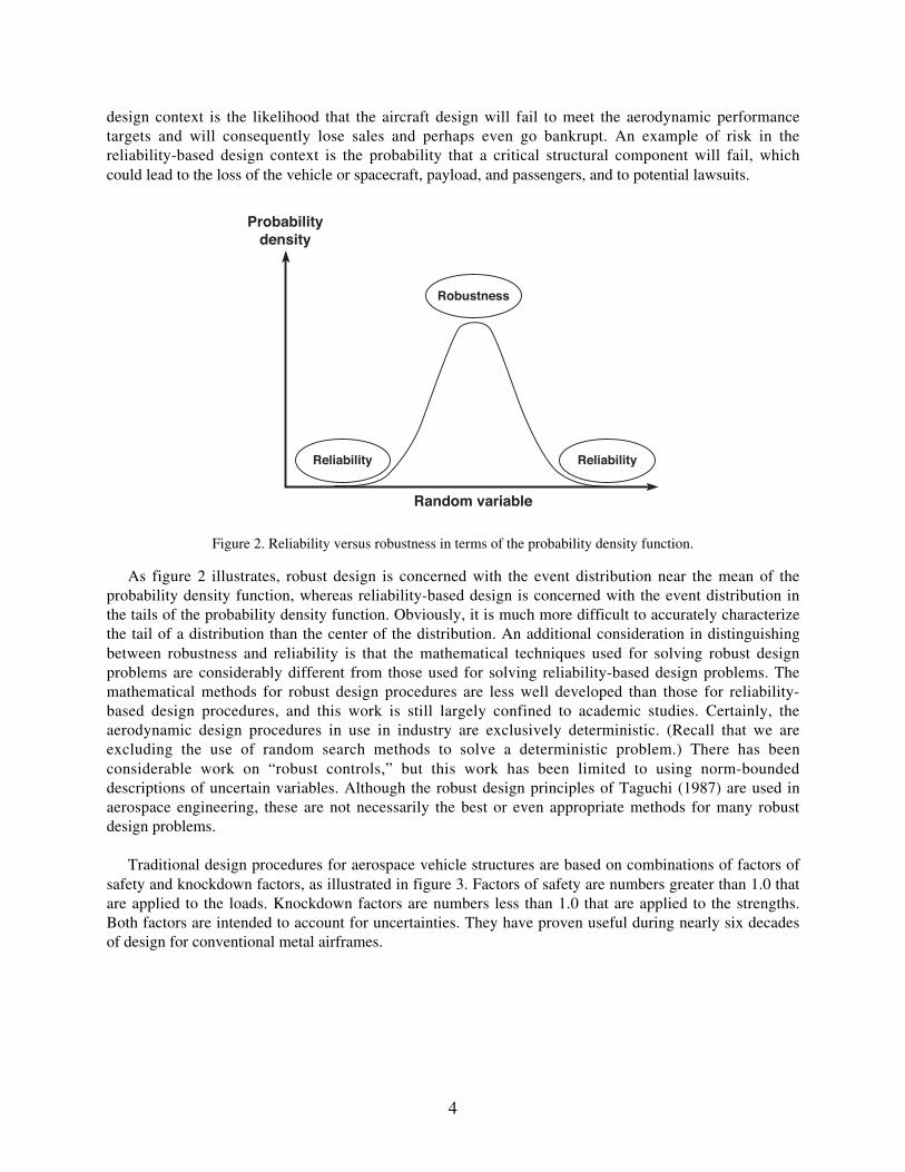
design context is the likelihood that the aircraft design will fail to meet the aerodynamic performancetargets and will consequently lose sales and perhaps even go bankrupt. An example of risk in thereliability-based design context is the probability that a critical structural component will fail, whichcould lead to the loss of the vehicle or spacecraft, payload, and passengers, and to potential lawsuits.

Random variable

Robustness

Reliability Reliability

Probabilitydensity

Figure 2. Reliability versus robustness in terms of the probability density function.

As figure 2 illustrates, robust design is concerned with the event distribution near the mean of theprobability density function, whereas reliability-based design is concerned with the event distribution inthe tails of the probability density function. Obviously, it is much more difficult to accurately characterizethe tail of a distribution than the center of the distribution. An additional consideration in distinguishingbetween robustness and reliability is that the mathematical techniques used for solving robust designproblems are considerably different from those used for solving reliability-based design problems. Themathematical methods for robust design procedures are less well developed than those for reliability-based design procedures, and this work is still largely confined to academic studies. Certainly, theaerodynamic design procedures in use in industry are exclusively deterministic. (Recall that we areexcluding the use of random search methods to solve a deterministic problem.) There has beenconsiderable work on “robust controls,” but this work has been limited to using norm-boundeddescriptions of uncertain variables. Although the robust design principles of Taguchi (1987) are used inaerospace engineering, these are not necessarily the best or even appropriate methods for many robustdesign problems.

Traditional design procedures for aerospace vehicle structures are based on combinations of factors ofsafety and knockdown factors, as illustrated in figure 3. Factors of safety are numbers greater than 1.0 thatare applied to the loads. Knockdown factors are numbers less than 1.0 that are applied to the strengths.Both factors are intended to account for uncertainties. They have proven useful during nearly six decadesof design for conventional metal airframes.

5

Figure 3. Factor of safety approach.

Traditional design procedures have several shortcomings. First, these procedures may be difficult toapply to aerospace vehicles that have unconventional configurations and that use new material systems.Second, measures of reliability and robustness are not provided in the design process. Consequently, it isnot possible to determine (with any precision) the relative importance of various design options on thereliability and robustness of the aerospace vehicle. In addition, with no measure of reliability it is unlikelythat the level of reliability and performance will be consistent throughout the vehicle. That situation canlead to excess weight with no corresponding improvement in overall reliability. Moreover, the factor ofsafety approach is logically inconsistent. It attempts to scale conditions using a mean or “worst-case”condition. In reality, a worst-case condition is rarely identifiable.

Figure 4. Reliability-based design approach.

In contrast to the traditional design procedure shown in figure 3, figure 4 illustrates how uncertaintiesare handled in the reliability-based design approach. Here both the load and the strength are characterizedby probability density functions. These distributions are due to uncertainties in the loads applied to thesystem (or subsystem) and to the strengths of different realizations of the system. The overlap region(where the load exceeds the strength) indicates the probability of failure. Note that for design of systemswith small probabilities of failure, the tails of both the load and the strength distributions are the mostrelevant. Reliability-based design methods have been used within civil engineering (Sundararajan 1995)for decades1 and in aircraft engine design (Cruse 2001) for about a decade. Applications to the structuraldesign of airframes are only now starting to emerge. Only academic studies of reliability-based designmethods within the aerodynamics and controls disciplines are known to the authors.

1 Civil engineering projects are generally designed using standard design codes. Many of these codes contain factorsthat can be adjusted based on the likelihood of occurrence of high loads or critical events, such as an earthquake of aspecified magnitude. These factors provide the target reliability. The probabilistic aspects of these design codes maybe hidden from the designer.

Load

Resistance(strength)

Load or resistance

Probabilitydensity

Failure (overlap region)

Load Resistance

Calculated

Factor of safety

Calculated

Knockdown factor

Margin

6

Newly emerging uncertainty-based design procedures will help to overcome the shortcomings of thetraditional design procedures. In particular, measures of reliability and robustness will be available duringthe design process and for the final design. This information will allow the designer to produce aconsistent level of reliability and performance throughout the vehicles—with no unnecessary over-designs in some areas. As a result, designers will be able to save weight while maintaining reliability. Inaddition, with an uncertainty-based design procedure it will be possible to determine the sensitivity of thereliability to design changes that can be linked to changes in cost. As a result, it will be possible to maketrade-offs between reliability and cost. For the same cost, airframes can be made safer than withtraditional design approaches—or, for the same reliability, the airframe can be made at a lower cost.

This white paper consists of a survey of the state of the art in uncertainty-based design together withrecommendations for a Base research activity in this area for the NASA Langley Research Center. Inparticular, section 2 provides a generic overview of current uncertainty-based design methods. Section 3focuses on uncertainty-based methods for aerospace vehicle design, describing the status of these methodsand the barriers to their adoption. Section 4 proposes some specific research objectives with both short-term and long-term impact on industry and NASA design processes. Section 5 discusses the expectedresults from uncertainty-based design research. Our discussion is limited to the disciplines ofaerodynamics, controls, structures, and systems analysis. Although other disciplines are excluded fromthe discussion, the reader will note that the authors have a diverse background, not just in terms of theirdisciplinary heritage but also in terms of their particular penchants towards experimentation, methodsdevelopment, or applied computation. This diversity, combined with the relatively recent interest of mostof the authors to this particular field of uncertainty-based design, has inevitably led to different emphasesin the different disciplinary sections of this report and perhaps to occasional inconsistencies interminology. The authors’ views on this challenging subject are a work in progress. They have chosen toput their current thinking out for comment now rather than wait the several years necessary for a fullmeeting of their minds.

2. Overview of Available Uncertainty-Based Design MethodsThe use of uncertainty-based design methods requires that the various uncertainties associated with the

design problem be characterized and managed, and that the analysis and optimization methodsincorporate this characterization of the uncertain quantities. In section 2.1 we focus on thecharacterization and management of uncertainties, and in section 2.2 we focus on the use of uncertaintiesin design.

2.1. Characterizing and Managing Uncertainties

Characterization and management of uncertainties is required at the individual discipline level as wellas at the integrated, system level. These involve the computational and experimental uncertaintiesproduced by the discipline analysis methods themselves, and the relationship of the uncertainties affectingthe input with the uncertainties affecting the output of the methods.

2.1.1. Computational Uncertainties

In the context of computational modeling and simulation, two complementary categorizations ofuncertainties are useful. One categorization distinguishes between parameter uncertainties and model

7

form uncertainties.2 Parameter uncertainties, sometimes referred to as parametric uncertainties orparameter variability, are those uncertainties associated either with the input data (boundary conditions orinitial conditions) to a computational process or with basic parameters that define a given computationalprocess, such as the coefficients of phenomenological models. Model form uncertainties, sometimesreferred to as structural uncertainties, nonparametric uncertainties, or unmodeled dynamics, are associatedwith model validity, i.e., whether the nominal mathematical model adequately captures the physics of theproblem.

Oberkampf et al. (1998) categorized uncertainties into three distinct classes. Variability refers to “theinherent variation associated with the physical system or the environment under consideration.”Uncertainty is “a potential deficiency in any phase or activity of the modeling process that is due to lackof knowledge.” Error is “a recognizable deficiency in any phase or activity of modeling and simulationthat is not due to lack of knowledge;” an error may be either an acknowledged error or anunacknowledged error. The value of this categorization is that the approaches to characterizing andmanaging uncertainties are considerably different for the three classes. We are not going to emphasizethis distinction in this white paper, and the interested reader should consult Oberkampf et al. (1998) formore information. In the material that follows, we shall typically use uncertainty in the more generalsense. Whenever we mean the more specialized definitions of this paragraph, we shall use italics for theterms.

In the context of a computer code used for computational modeling and simulation, the parameteruncertainties can be specified by means of interval bounds, membership functions, or probability densityfunctions, as illustrated in figure 5. Interval bounds should be used when only the crudest information isknown. They use only an upper and a lower bound for the parameter value; norm-bounded uncertaintiesare a special case. Probability density functions are the most detailed description. Membership functions,which are used in fuzzy logic approaches, provide an intermediate level of detail. The parameteruncertainty characterization can be based on expert opinion, experimental data, analytical estimates, orresults from upstream computational processes. A more detailed discussion of the general mathematicalframework for characterization of uncertainties from an engineering perspective can be found inOberkampf, Helton, and Sentz (2001).

Uncertain variable

Interval bound

1.0

Uncertain variable

Possibility

Membership function

Uncertain variable

Probabilitydensity

Probability density function

Area = 1.0

Figure 5. Uncertainty descriptions.

Strategies for characterization of model form uncertainty are far less well developed than those for 2 The terms model uncertainty and modeling uncertainty are occasionally used in the literature to mean theuncertainty in the model arising both from the model form and the model parameters. These terms should not beconfused with the term model form uncertainty as we are using it here.

8

parameter uncertainties. Two general references of note are Beck (1987) and Draper (1995). A shortsummary of the Bayesian approach to model form uncertainty, together with some additional references,is given by Alvin et al. (2000). There do not appear to be any systematic applications of model formuncertainty characterization strategies to airframe design applications.

Few systematic approaches are available for managing uncertainties in computational simulations.Adaptive mesh refinement is the most well developed, but most techniques are based on heuristic ratherthan rigorous approaches. Moreover, adaptive mesh refinement is limited to just one aspect of theuncertainty in the output of a code (discretization error) and it does not address the uncertainty in themodel output due to uncertainty in the model input.

2.1.2. Experimental Uncertainties

The traditional approach to account for uncertainties in structural design is to introduce so-calleddesign or safety factors on the loads and statistically based material properties. Thus, in a classicaldeterministic analysis, all the uncertainties are accounted for in a “lump-sum” fashion by multiplying themaximum expected applied stress by a single safety factor, e.g., 1.5. The specification of safety factors isgenerally based on empirical design guidelines established from years of structural testing and experience.Statistically based material properties are determined from a series of coupon tests. Design verification isachieved through testing by applying the worst-case loading condition to the structure and testing tofailure.

Uncertainties can be accounted for using probabilistic methods. Techniques for deriving probabilisticinformation and for estimating parameter values from observed data are found in the methods ofstatistical inference in which information obtained from sample data is used to make generalizations aboutpopulations from which the samples were obtained. Traditional methods of estimation include point andinterval estimates. The common methods of point estimation are the method of maximum likelihood andthe method of moments. Interval estimation includes determining the interval that contains the parametervalue and a prescribed confidence level. However, when population parameters are estimated based onfinite samples, errors of estimation occur. Explicit consideration of these errors is accounted for in theBayesian approach to estimation. With this approach, subjective judgments based on intuition,experience, or indirect information are incorporated with observed data to obtain a balanced estimation.Validity of assumed uncertainty distributions is verified or disproved statistically by goodness-of-fit tests,such as chi-squares or Kolmogorov-Smirnov methods.

For situations in which sample data necessary to quantify parameter uncertainties is limited ornonexistent, fuzzy set (possibilistic) analysis can be used to account for uncertainties. Uncertainties areintroduced by specifying membership functions.

Systematic procedures for characterizing and managing3 uncertainties in experimental activitiesinclude design of experiment methods (Taguchi 1987) and statistical process control techniques (Wheelerand Chambers 1992). The former focuses more on characterizing the uncertainties and the latter more onmanaging them.

2.1.3. Uncertainty Analysis

The objective of uncertainty analysis (or uncertainty propagation) is to characterize the uncertainties in

3 Although in this context the word "control" is more conventional, we prefer the term "manage" to preventconfusion with the "controls" discipline.

9

the system output given some knowledge of the uncertainties associated with the system parameterstogether with one or more computational models and, ideally, some experimental data. This subsectionwill provide an overview various approaches to estimating the effects of parameter uncertainties;approaches to model form uncertainties are far less developed. Several methods are available forestimating the uncertainties in the performance predictions due to parameter uncertainties. They depend,of course, on whether the parameter uncertainties are specified in terms of probability density functions,membership functions, or interval bounds.

2.1.3.1. Probabilistic Analysis. The most well developed approaches to uncertainty analysis are based onparameter uncertainties specified in terms of probability density functions (PDFs). Uncertainty-baseddesign methods using detailed PDFs are generally referred to as probabilistic methods. In this case, theuncertainty computing engine produces the nominal value of the performance functions as well as theirPDFs. This process is typically completed by using some type of Monte Carlo or statistical samplingmethod. The concept is straightforward; the process model is invoked repeatedly for deterministicanalyses performed for a set of input parameters generated according to their PDFs to produce a set ofoutput samples. The statistical properties of the output performance functions are then deduced from theoutput samples. This approach is usually referred to as a simulation method or a sampling method. SeeMelchers (1999) for a general overview. The simplest approach is the basic Monte Carlo method, inwhich the sampling points are drawn strictly according to the PDFs of the input parameters. Constructionof accurate output PDFs can easily take thousands or even millions of simulations. Two of the morepopular alternatives to the basic Monte Carlo method are Importance Sampling and Latin HypercubeSampling (McKay, Beckman, and Conover 1979). The former enables accurate estimates of the tails ofthe PDFs; it is most useful in reliability-based design problems. The latter provides samples that ensurecoverage of the full range of the input parameters with far fewer simulations than the basic Monte Carlomethod. However, the tails of the output PDFs are generally quite inaccurate; it is most useful in robustdesign problems. Yet another refinement is Directional Sampling, which is useful for concentrating thesampling on a subset of the parameters of particular interest. At least a half-dozen general-purposecommercial software packages are available to serve as probabilistic uncertainty computing engines.

A different approach to probabilistic uncertainty analysis is by the solution of stochastic differentialequations. With this approach, the uncertainties may be associated with initial conditions, boundaryconditions, transport properties, and source terms. Wiener (1938) developed a method of representing theassociated randomness in the solution with an expansion in orthogonal polynomials in which the burdenof representing the random component is carried by the polynomials; the coefficients of the expansion aresmooth functions. Ghanem and Spanos (1991) and Ghanem (1999) refined Wiener’s method and appliedit to structural analysis problems. Xiu and Karniadakis (2001) have generalized the class of expansionfunctions and applied it to fluid mechanics and fluid-structures problems; they have shown that the set ofWiener-Askey polynomials contains an appropriate (and rapidly convergent) polynomial family for manyof the PDFs of physical interest. This approach is referred to as Polynomial Chaos. One obtains the PDFsof every component of the solution at every space-time point. The cost is typically one to two orders ofmagnitude greater than that of a deterministic solution for the differential equation, yet is still orders ofmagnitude cheaper than required for an ensemble of solutions generated by a Monte Carlo method.

2.1.3.2. Fuzzy Logic. When the parameter uncertainties are characterized by membership functions, fuzzylogic is the basis for assessing the uncertainties in system output. Fuzzy logic allows one to create modelsbased on inexact, incomplete, or unreliable knowledge or data, and, moreover, to infer approximatebehavior of the system from such models. Fuzzy logic provides a computational engine to process thesemodels (Harris, Moore, and Brown 1993). To date, fuzzy logic has found many applications in controls,manufacturing, pattern recognition, and even finance (Holmes and Ray 2001; Ham, Qu, and Johnson2000; Inoue and Nakaoka 1998; Isermann 1998; Dexter 1995; Hung 1995; Lim and Hiyama 1991; Lee

10

1990; Box and Draper 1987). Fuzzy logic is an extension of multivalued logic. Its predicates can be bothcrisp (not fuzzy), such as numbers, or true and false, and non-crisp (fuzzy), such as greater than, small,etc. Uncertainty characterizations using membership functions are sometimes referred to as possibilistic,which is often used to contrast this approach with the probabilistic approach.

The central concept of fuzzy logic is the membership function, which represents the degree ofmembership of the fuzzy variable within the fuzzy set (Harris, Moore, and Brown 1993). The membershipfunction may be thought of as a possibility function in contrast to the probability density function inprobability theory. In fuzzy logic, input and output mappings are established through fuzzy algorithmsbased on a collection of rules, in the form of conditional statements. The composition of an inputvariable(s) with the fuzzy rules (relations) produces a fuzzy set for the output. To obtain a crisp output,the fuzzy set has to be de-fuzzified to a single value; different techniques can be used to accomplish thistask.

Fuzzy logic is appealing for its simplicity of application and implementation. It may be useful inapplications wherein accurate physical models are not available, for preliminary design and analysis, or incases wherein crude or fuzzy inferences and actions are acceptable. However, in uncertainty-based designand analysis, the use of fuzzy logic may be confined to the conceptual design and early preliminarydesign stages; the level of accuracy required in most aerospace applications in late preliminary anddetailed design is far too stringent to allow for fuzzy logic.

2.1.3.3. Interval Analysis. Interval analysis was initially developed to account for errors in floating pointarithmetic. The chief distinguishing element of its framework is that variables are represented by twoscalars: a lower bound value and an upper bound value. These numbers reflect a measure of uncertainty inthe knowledge of the actual value of the variable. Interval arithmetic involves the rules developed toperform mathematical operations with interval numbers. Interval analysis is ideally suited to deal withparametric uncertainties in systems. In its simplest form, a combinatorial analysis is used to constructinterval distributions of the performance quantities. It has been applied in a variety of fields, includingstructural analysis and dynamic analysis, to accommodate uncertainties in parameters (Piazzi and Visioli2000; Jaulin and Walter 1997; Oppenheimer and Michel 1988; Ugur Koyluoglu and Elishakoff 1998;Qiu, Chen, and Elishakoff 1995; Rao and Berke 1997). However, these applications involve mainlysimple problems of small order. Applications to medium-large size problems are lacking because bynature, interval arithmetic produces potentially conservative results, i.e., the results are not practical. Thelevel of conservatism may be reduced if interval variables and arithmetic are used in closed-formsolutions of the problem output, as opposed to throughout the numerical solution. Unfortunately, closed-form solutions are rarely available, except for the simplest of problems. Another minor problem withinterval analysis is that it is computationally more expensive than traditional mathematics since it dealswith intervals and not just scalars. However, with recent advancements in computing technology, thishigher computational expense is not an issue anymore. In fact, interval arithmetic is accommodated in thelatest SUN Microsystems Forte Fortran 95 Compiler. One other potential problem is that interval analysismay not be amenable to accommodating correlated uncertainty distributions. This issue may lead toadditional conservatism in the predictions of bounds for the system output.

2.1.4. Sensitivity Analysis

Sensitivity analysis is related to, but different from, uncertainty analysis. The recent book edited bySaltelli, Chan, and Scott (2000) provides thorough coverage of this vast subject. The overview chapter byCampolongo et al. (2000) defines sensitivity analysis as “the study of how the variation in the output of amodel (numerical or otherwise) can be apportioned, qualitatively or quantitatively, to different sources ofvariation, and of how the given model depends upon the information fed into it.” As used here, sensitivity

11

analysis ascertains which parameters have the greatest influence on the system output. It is a deterministicquestion. Its primary relation to uncertainty analysis is to enable the identification of which parametersreally matter—conducting an analysis of the impact of the uncertainty of a parameter that has aninsignificant effect upon the performance measures is futile. Given the high cost of most uncertaintyanalysis methods, it usually pays to first conduct a sensitivity analysis to weed out consideration ofunimportant parameters. This process is often “step 0” in the construction of a response surface.

Campolongo et al. (2000) list three general approaches to sensitivity analysis with numerical models.Factor screening determines which parameters (or groups of parameters) have the greatest impact on themodel output variability. Various design of experiment techniques are typically employed. These consistof evaluating model output at the extreme values of the ranges of the parameters. Local sensitivityanalysis utilizes first-order derivatives of model output quantities with respect to the parameters. Likefactor screening, local sensitivity analysis is a deterministic calculation, but it is usually performed for anominal set of parameter values. Some computational tools provide accurate and efficient sensitivityderivatives, but in most cases costly (and sometimes inaccurate) finite-difference approximations are usedto compute the derivatives. Global sensitivity analysis typically uses statistical sampling methods, such asLatin Hypercube Sampling, to determine the total uncertainty in the model output and to apportion thatuncertainty among the various parameters.

If efficient sensitivity derivatives for the model are available, then local sensitivity analysis is by farthe least costly in terms of computational time. At worst, its cost increases linearly with the number ofparameters. However, it is limited to the vicinity of the nominal parameter values. The cost of factorscreening methods that look at one factor at a time increases linearly with the number of parametervalues, whereas methods that look at the full set of mutual interactions have an exponentially increasingcost. Statistical sampling approaches typically require thousands of evaluations of the computationalmodel, although their cost is in principle independent of the number of parameters. This approach isprohibitively expensive for models with nontrivial computational times. The only feasible approach forthis important class of models is to generate an approximation to the model, and then to perform thestatistical sampling on the approximation. Constructing such an approximation, however, is only feasiblefor a small number of parameters.

2.1.5. Approximations

Clearly, the methods described previously for uncertainty propagation and for sensitivity analysis areimpractical when the computational time required to evaluate the process model is large. This problem isusually dealt with by using approximations. Several alternatives to sampling methods have beendeveloped for estimating the PDF of the performance function. The Advanced Mean Value method (Wuand Wirsching 1989) exploits a first-order approximation to the performance function together with a FastProbability Integration technique. The first-order approximation requires the computation of the gradientsof the performance function with respect to all the random variables. The Fast Probability Integration thenperforms an integration over this linear approximation. Field, Paez, and Red-Horse (1999) have improvedthis method to yield more accurate moments of the PDF. Du and Chen (2000a) have developed a methodbased on Most Probable Point techniques for efficiently constructing the PDF. It, too, utilizes the first-order derivatives of the performance function. Both of these methods are usually implemented with finite-difference approximations to the gradients of the performance functions. Their cost can be dramaticallylower if efficient methods for computing these derivatives are exploited.

More generally, one can build an approximation, typically a response surface model, for the exactprocess model. The response surface is then used in lieu of the exact process model by the uncertainty

12

computing engine. Response surface approximations are constructed by the following three steps:

• Experiment points are selected.

• Response surface model order is selected.

• Experiment points are fitted to the chosen model.

The selected experiment points determine where in the design space the exact process model will beevaluated. Design of experiment techniques are typically employed; for an excellent treatment on theselection of the experiment points see Box and Draper (1987). When selecting the response surface modelorder, quite often either linear or quadratic surfaces are assumed. Once the model order has beendetermined, the response surface is fit using least squares. In some cases the model order is not selectedbeforehand; instead the response surface model is chosen such that the first two statistical moments of theresponse surface match that of the exact process model, resulting in first-, second-, or even higher-ordersurfaces.

2.2. Analysis and Optimization Incorporating Uncertainties

The previous subsection focused on methods for describing the uncertainties in the performancemeasures of a discipline or system. This description may be in the form of probability density functions,membership functions, or interval bounds. In this subsection, we discuss methods that use thisinformation in design, e.g., by computing failure probabilities, by design of control systems, or byoptimizing a system in the presence of uncertainties.

2.2.1. Impact of Uncertainty on Performance Measures

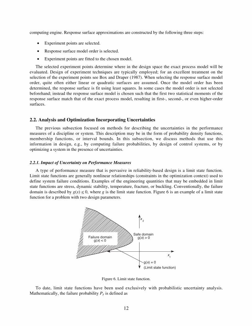
A type of performance measure that is pervasive in reliability-based design is a limit state function.Limit state functions are generally nonlinear relationships (constraints in the optimization context) used todefine system failure conditions. Examples of the engineering quantities that may be embedded in limitstate functions are stress, dynamic stability, temperature, fracture, or buckling. Conventionally, the failuredomain is described by g(x) < 0, where g is the limit state function. Figure 6 is an example of a limit statefunction for a problem with two design parameters.

Failure domainSafe domain

g(x) < 0g(x) > 0

g(x) = 0

x1

x 2

(Limit state function)

Figure 6. Limit state function.

To date, limit state functions have been used exclusively with probabilistic uncertainty analysis.Mathematically, the failure probability PF is defined as

13

P P g X f x dxF X

g x

= ( ) ≤[ ] = ( )( )≤∫0

0

(1)

where fX(x) is the joint probability density function of X and the integration is carried out over the entirefailure domain. For many engineering applications, solving equation (1) may entail a substantialcomputational effort. Some of the difficulties in evaluating the right-hand side of equation (1) include:

• High dimensionality of the design space makes the integration very costly

• Mathematical and computational complexity of the domain boundaries given by g(x) = 0

• Lack of information regarding the joint probability density, fX(x)

Because of these complexities, exact solutions of failure probabilities for general systems witharbitrary parameter uncertainty PDFs are not feasible; therefore, efficient numerical methods forcomputing approximate failure probabilities are required. In fact, the development of efficientapproximate numerical techniques has been the subject of much research.

The goal of First-Order Reliability Methods (FORM) and Second-Order Reliability Methods (SORM)is to compute failure probabilities efficiently by exploiting approximate forms of the limit state function.FORM and SORM replace the limit state function in equation (1) with first-order and second-orderapproximations, respectively. FORM and SORM reliability methods consist of four basic computationalsteps:

1. Transform from physical space to standard normal space.

2. Determine the most probable point (MPP).

3. Approximate the limit state function at MPP.

4. Compute the failure probability using the approximated limit state function from step 3.

Step 1 is particularly important because of the properties of standard normal space. The mostimportant property of standard normal space in regards to computing failure probabilities is thatprobability densities decay exponentially with the square of the distance from the origin. Therefore if oneapproximates the limit state function in the vicinity of the MPP (the closest point to the origin), themajority of the failure probability will be captured by an approximate limit state function because it ismost accurate in the region that contributes the most to the integration. The specifics for computingfailure probabilities for FORM and SORM differ slightly, but the primary difference between them is theorder of the approximated hypersurface. In FORM, the limit state function is approximated by a tangenthyperplane at the MPP; in SORM, a quadratic hypersurface is used. This difference generally results inSORM producing more accurate estimates of failure probabilities, but at the cost of greater computer timedue to the second-order gradient computations.

Rackwitz (2000) has written a detailed review of FORM and SORM methods. Thacker et al. (2001)have provided a useful description of the weaknesses of current FORM and SORM algorithms. Thacker etal. (2001) note that Importance Sampling Methods are often used to increase the accuracy of the limitstate function probabilities near the MPP. Choi and Youn (2001) have recently developed an alternativeapproach to reliability analysis that inverts the objective and constraint functions in the optimization usedto identify the MPP.

2.2.2. Bounded Uncertainty Design and Analysis

The controls community has developed a special approach that they refer to as bounded uncertainty

14

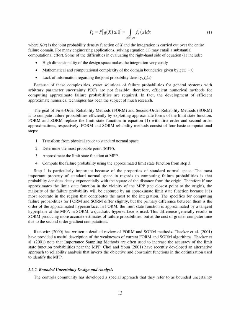
design and analysis. In this approach, system uncertainties can be either parametric or nonparametric.Furthermore, the uncertainties can be real or complex time-independent functions, or linear/nonlineartime-varying functions (Balas and Packard 1996; Doyle, Wall, and Stein 1982). No matter what form ofuncertainty one is dealing with, the uncertainty is assumed to be norm bounded, i.e., the maximumexcursions of uncertainties are assumed to be known a priori. Figure 7 is an example of how the boundeduncertainty is added to a system. In this figure, P is the plant, d represents the exogenous inputs (typicallyunknown disturbances or reference signals), yp are the sensor measurements, ∆∆∆∆ is the uncertainty block,and W and Z are used to define the interconnection between the plant and the uncertainty block.

W Z∆

P ypd

Figure 7. Bounded uncertainty structure.

The main objective in the Bounded Uncertainty Design and Analysis approach is to obtain bounds onthe potential variations in system performance based on the bounds on the parametric and nonparametricuncertainties. The type of analysis required in this approach can vary significantly from one application toanother. It can be simply a norm-based analysis in which the norm bounds at the uncertainty levels arepropagated through to the system performance, e.g., bounds on stress levels due to bounded uncertainty inthe material properties. Substantial work has been done for linear time-invariant dynamical systems inthis area (Balas and Packard 1996; Doyle, Wall, and Stein 1982; Moser 1993; Balas and Doyle 1994;Gagnon, Pomerleau, and Desbiens 1999; Bendotti and Beck 1999; Nishimura and Kojima 1999; Pannu etal. 1996; Cheng and De Moor 1994; Balas et al. 1998). Various techniques are available to incorporateparametric and nonparametric uncertainties within the linear system. Both structured and unstructureduncertainty models can be considered in this framework (Balas and Packard 1996). A structureduncertainty model denotes a model in which uncertainty is directly associated with specific parameters inthe system, while in the unstructured uncertainty model, uncertainties are general, and hence are notassociated with any specific parameter in the model. Several methods are available for analysis ofdynamic stability and performance of these systems. An example is the Linear Matrix Inequalityframework, which uses convex programming (Scherer, Gahinet, and Chilali 1997; Apkarian and Adams1998). The treatment of linear time-invariant systems with uncertainty can be extended to linear time-varying systems as well as a certain class of nonlinear systems (e.g., linear parameter varying systems)with the aid of the Linear Matrix Inequality framework (Scherer, Gahinet, and Chilali 1997; Apkarian andAdams 1998). For general nonlinear systems, the treatment of bounded uncertainties is somewhat ad hoc,as there are no formal methods for dealing with such systems. However, in some cases, Lyapunovstability theory and norm-based propagation can be used to establish bounds on the performance of thenonlinear system.

15

2.2.3. Optimization Under Uncertainty

Several design optimization methods include uncertainty. For the purpose of this paper, the methodscan be divided into three groups: sampling methods, robust optimization, and optimization for reliability.Sampling methods can be used to solve either robust optimization or reliability-based optimizationproblems, but we find it useful to discuss these methods separately. The sampling methods perform allexperiments (whether mathematical simulations or physical tests) simultaneously and then optimize thedesign based on the results of those experiments. Robust optimization methods use the numericaloptimization procedure to specify which simulations are needed and evaluate those simulations one at atime. The optimization for reliability methods also use numerical optimization procedures but with thegoal of reliability rather than robustness.

2.2.3.1. Sampling Methods. Sampling methods are based on the assumption that the designer will choosean optimum design by evaluating a performance or cost measure at a large number of points in designspace. Ideally, these points define a smooth hypersurface with a well-defined feasible region and a singleoptimum point. If the cost measure (also called objective function) includes parametric uncertainty, thenmany evaluations are required at each point in design space to accurately characterize the hypersurface.

Trouble arises when the value of the objective function is evaluated with a variety of differentcomputer simulations and experimental data. Each source of measured and computed data includes errors(e.g., due to simplification in the mathematical models) and uncertainty (e.g., due to the differencebetween the ensemble averages and the individual test results). For a good overview of available samplingand response surface approximation techniques see Robinson (1998). For a discussion of the types ofvariabilities, uncertainties, and errors found in simulation codes and for uncertainty estimation methodssee Alvin et al. (2000).

Conceptually, optimization that includes uncertainty can be achieved by fitting all available data withsome smooth surface and then using a mathematical optimization procedure to determine the best design.All sampling approaches considered here use the following three steps: (1) sample the design space, (2)approximate the objective function, and (3) estimate the optimum of the approximate surface. These stepscan be repeated one or more times on smaller and smaller neighborhoods surrounding the currentoptimum point.

Several popular techniques differ in steps (1) and (2). For example, the design space can be sampledusing Taguchi arrays, Latin hypercubes, random points, or some subset of available data. Similarly, theapproximate surface can be constructed using neural nets, polynomials, or splines under tension. Thechoice of method depends on knowledge of the design space (e.g., the objective function may varylinearly with respect to some design variables) and on the amount of available data.

Response surface methods (RSM) and Taguchi parameter design methods are the most commonlyused procedures. Venter and Haftka (1999) explain that RSM reduces the computational burden andsimplifies the integration of optimization and analysis codes. Roy (1990) and Nair (1992) discuss theTaguchi method and some of its known strengths and drawbacks. Unal, Stanley, and Joyner (1993)provide a good tutorial on Taguchi methods written from an engineering perspective. The principallimitations of both RSM and Taguchi parameter design methods are: neither constraints nor multipleobjective functions are accommodated; dimensionality restricts the application of these methods toproblems with a small number of parameters and design variables; and they are far less applicable touncertainty and error than to variability (as these terms are used by Oberkampf et al. 1998). AlthoughTaguchi methods are effective for many problems, work still needs to be done to develop alternativeapproaches that overcome these limitations.

16

2.2.3.2. Robust Optimization Methods. For our purposes, robust optimization methods seek to improve adesign by making it insensitive to small changes in the design values, and they exploit sequentialnumerical optimization techniques. One method for achieving robustness is to minimize both the meanand variance. Thus, the optimization problem is formulated as a multiobjective problem:

tw c t w t

∈+

Ωmin ( , ) ( , )

1 22θ σ θ (2)

where t are the design variables in the domain Ω, θ are the uncertain parameters that are described by oneor more PDFs, c is the mean of the objective function, σ2 is the variance of c due to the randomness of θ,and wi are the user-defined weights. Depending on the choice of weights, this formulation will minimizethe objective, minimize the variance in the objective, or discover some compromise between these twogoals.

Robust optimization methods are effective if c(t,θ) is a good simulation of the performance or costgoals and if the PDF of θ is well characterized. For example, structural analysis codes can accuratelypredict the strains in metal truss structures given the loads. Moreover, the PDF of uncertain loadingparameters such as wind speed or wave height have been collected. Therefore, robust optimization forsizing of civil engineering projects should result in safer and more cost-effective structures.Unfortunately, few simulation codes automatically predict the variance of the mean given a known PDFof the uncertain parameters. Tada, Matsumoto, and Yoshida (1988) provide a clear explanation of thismethod and its application to simple structural sizing problems.

2.2.3.3. Optimization for Reliability. Optimization for reliability methods are based on the assumptionthat the design space is divided into two regions: success and failure. The goal of the optimization is tofind the best design that is sufficiently far from the failure region so that the probability of failure isacceptably small. Thus, the optimization problem is formulated as a constrained optimization problem:

tc t

∈( )

Ωmin ,θ (3)

subject to

P g t r,θ( ) ≤[ ] ≤0 (4)

where r is the reliability requirement, g(t,θ) = 0 defines the boundary (or limit surface) between successand failure, and P[g ≤ 0] is the probability of failure for the current values of the design vector t.

Optimization for reliability can be attempted using standard constrained nonlinear optimizationprocedures. The major difficulty is the computational expense of calculating the probability of failure. Asecondary difficulty is that the constraint PF ≤ r can be a highly nonlinear function of t even if g(t,θ) islinear in t.

The computational expense of optimization for reliability greatly hinders its acceptance. If anevaluation of the constraint g(t,θ) is computationally expensive or if the reliability requirement r is small,then Monte Carlo analysis can be prohibitively expensive since it requires thousands of evaluations of g atrandomly sampled values of θ. An alternate approach is to (1) use the optimization code to find the mostprobable point of failure or MPP, (2) estimate the probability of failure using a linear approximation tothe limit surface centered at the MPP, and (3) use the optimization code to minimize the objective for therequired probability of failure. In this alternate approach, the optimization code is used twice, first to find

17

the values of θ that define the MPP and then to find the values of t which reduce the objective withoutcompromising safety. See Langley (2000) and Grooteman (1999) for a good overview of these methods.

3. Current Status and Barriers

3.1. Structural Analysis

3.1.1. Current Status

Traditionally, the approach to designing aerospace structures with uncertainties is to use statisticallybased material properties (e.g., yield strength) and to introduce design factors. The statistically basedmaterial properties are characterized as A-basis and B-basis material property values (Anon. 1997). An A-basis material property is one in which 99 percent of the material property distribution is above the basisvalue with a 95 percent level of confidence. A B-basis material property is one in which 90 percent of thematerial property distribution is above the basis value with a 95 percent level of confidence. Designfactors can be placed into two categories and include safety factors and design knockdown factors forstability critical structures. Safety factors account for uncertainties in a “lump-sum” fashion bymultiplying the maximum expected applied stress by a single safety factor. The FAA air-worthinesscertification requires a design safety factor equal to 1.5 for man-rated aircraft structures; however, safetyfactors as low as 1.02–1.03 have been used in the past for non-man-rated structures such as missiles. Thesafety factor is intended to account for uncertainties such as uncertainty in aerodynamic load definitionand structural stress analysis, variations in material properties due to manufacturing defects andimperfections, and variations in fabrication and inspection standards. The safety factor is generallydeveloped from empirically based design guidelines established from years of structural testing ofaluminum structures. For a historical review of the evolution of the 1.5 factor of safety in the UnitedStates, see Muller and Schmid (1978).

The traditional approach to designing thin-walled buckling-resistant structures is to predict thebuckling load of the structure with a deterministic analysis and then to reduce the predicted load with anempirical design knockdown factor, which is intended to account for the difference between the predictedbuckling load and the actual buckling load of the structure determined from tests. The differencesbetween analysis and test results are mainly due to uncertainties in the structural geometry (e.g.,imperfections), loading conditions, material properties, and boundary conditions. Design guidelines forstability critical isotropic structures can be found in several NASA documents including Weingarten,Seide, and Peterson (1968) for buckling of thin-walled circular cylinders, Weingarten and Seide (1968)for buckling of thin-walled truncated cones, and Weingarten and Seide (1969) for the buckling of thin-walled doubly curved shells.

Many of the aforementioned design practices have been carried over to composite structures for lackof better design methods. In addition, these design methods can potentially result in overly conservativeor unconservative designs of aerospace structures. Furthermore, these design guidelines do not includeany data or information related to uncertainty sensitivity.

3.1.1.1. Probabilistic Analysis and Design Methods. A probabilistic design methodology reported inAnon. (1997) accounts for uncertainties in material properties; external or operational loads;manufacturing processes and their effects on material strength; environmental effects on strength such asmoisture or radiation exposure; environmental history during operation; flaw and/or damage locations,

18

severity, and probability of occurrence and effects on strength; and predictive accuracy of structuralmodels and analysis. The probabilistic approach uses the statistical characterization of parameteruncertainties and attempts to provide a desired reliability in the design. In the probabilistic approach, theuncertainties of the individual design parameters and loads are modeled by appropriate probabilitydensities. These probability densities are combined into cumulative density functions by usingtransformation equations. In this case, the design parameters have an uncertainty that is quantified interms of risk. The credibility of this approach depends on two factors: the accuracy of the analyticalmodel used to predict the structural response, and the accuracy of the probabilistic techniques employed.This probabilistic methodology has shown some success in the design of composite structures where theparameter uncertainties are well-known. For example, the IPACS (Integrated Probabilistic Assessment ofComposite Structures) computer code was developed at NASA Glenn Research Center (Chamis andMurthy 1991), and a probabilistic stability analysis for predicting the buckling loads of compression-loaded composite cylinders was developed at Delft University of Technology (Arbocz, Starnes, andNemeth 2000).

3.1.1.2. Fuzzy Set or Possibilistic Analysis Methods. For situations in which sample data necessary toquantify parameter uncertainties are limited or nonexistent, fuzzy set analysis can be used to account foruncertainties. In these methods, uncertainties in input parameters (e.g., dimensions, Young’s modulus) aredefined by membership functions. An example of a membership function is shown in figure 8.

1.0

Uncertain quantity

Possibility

.20 .25 .300

Figure 8. Example of membership function.

The vertical scale is the possibility that an uncertain quantity takes on a given value, and the horizontalscale shows values of the uncertain quantity. The possibility varies from zero (no possibility) to one(maximum possibility). In this example, the most likely value of the uncertain quantity is 0.25. Theuncertain quantity is bounded by 0.20 and 0.30 at Possibility = 0.0. The objective is to use themembership functions of the input parameters to determine the corresponding membership functions forthe response quantities (e.g., stress, buckling load). The membership functions for the response quantitiesare then compared with the membership functions of the allowable responses to determine the possibilityof failure.

A subset of fuzzy set or possibilistic analysis is sometimes called interval analysis. In this approach,upper and lower bounds are placed on the uncertain input parameters, and the resulting upper and lowerbounds are calculated for the response quantities. The objective is merely to bound the response rather

19

than to indicate the likelihood of the response taking on a given value. This approach is equivalent toworking with membership functions at a possibility of zero.

Fuzzy set or possibilistic analysis methods have been proposed by Noor, Starnes, and Peters (2000)and have been applied to structural problems such as the probabilistic strength predictions of bondedjoints by Stroud, Krishnamurthy, and Smith (2001). In addition, interval analysis has been used to predictresponse bounds for compression-loaded composite shells with random imperfections, e.g., Hilburger andStarnes (2000).

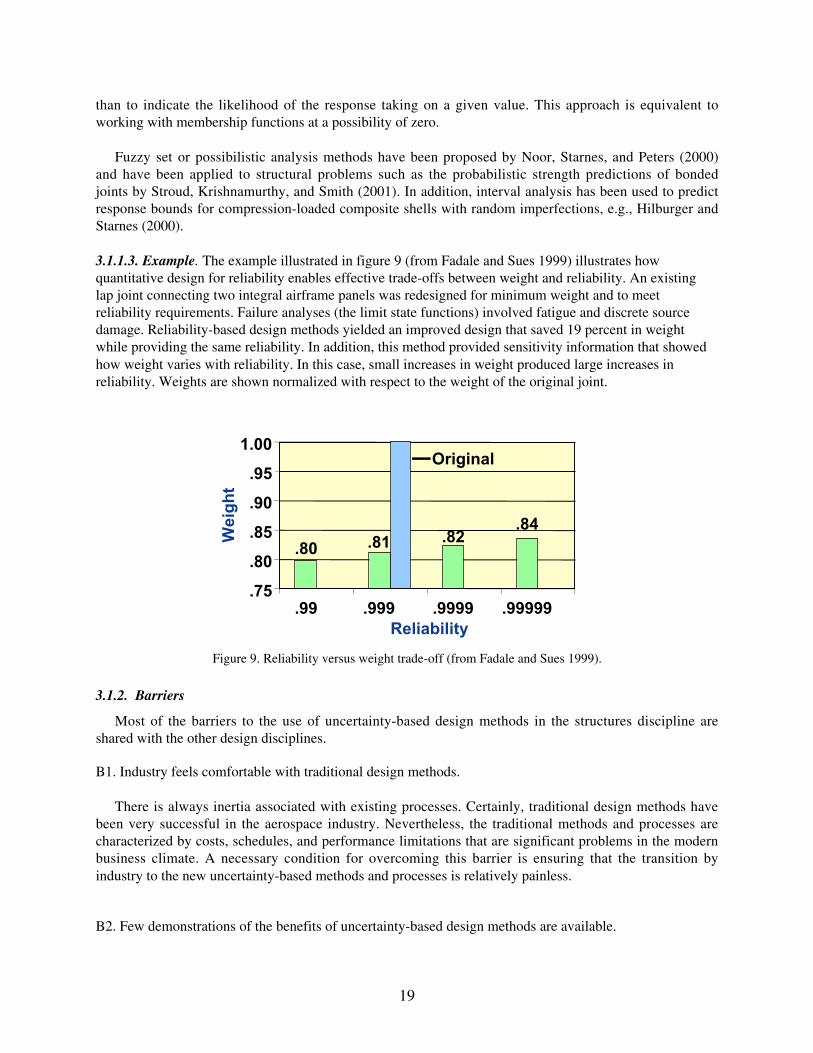
3.1.1.3. Example. The example illustrated in figure 9 (from Fadale and Sues 1999) illustrates howquantitative design for reliability enables effective trade-offs between weight and reliability. An existinglap joint connecting two integral airframe panels was redesigned for minimum weight and to meetreliability requirements. Failure analyses (the limit state functions) involved fatigue and discrete sourcedamage. Reliability-based design methods yielded an improved design that saved 19 percent in weightwhile providing the same reliability. In addition, this method provided sensitivity information that showedhow weight varies with reliability. In this case, small increases in weight produced large increases inreliability. Weights are shown normalized with respect to the weight of the original joint.

Figure 9. Reliability versus weight trade-off (from Fadale and Sues 1999).

3.1.2. Barriers

Most of the barriers to the use of uncertainty-based design methods in the structures discipline areshared with the other design disciplines.

B1. Industry feels comfortable with traditional design methods.

There is always inertia associated with existing processes. Certainly, traditional design methods havebeen very successful in the aerospace industry. Nevertheless, the traditional methods and processes arecharacterized by costs, schedules, and performance limitations that are significant problems in the modernbusiness climate. A necessary condition for overcoming this barrier is ensuring that the transition byindustry to the new uncertainty-based methods and processes is relatively painless.

B2. Few demonstrations of the benefits of uncertainty-based design methods are available.

.80 .81 .82.84

Original

.75

.80

.85

.90

.95

1.00

.99 .999 .9999 .99999

Weight

Reliability

20

The technology advocates of uncertainty-based design need to provide compelling demonstrations ofthe benefits of uncertainty-based design methods and a compelling business case for changing to the newprocesses. This case must demonstrate measurable benefits and must be couched in terms readilyunderstandable by both technology managers and practitioners. Given the head start of the structurescommunity on uncertainty-based design methods, this barrier is even greater for the other designdisciplines.

B3. Uncertainty-based design methods are more complex and considerably more expensive thandeterministic design methods.

Advances in computer hardware and software, especially in automation, are bound to help. However,orders of magnitude improvements are needed to overcome this barrier. Fundamental breakthroughs areneeded in this area.

B4. Characterization of structural imperfections and uncertainties necessary to facilitate accurate analysisand design of the structure is time-consuming and is highly dependent on structural configuration,material system, and manufacturing processes.

To some extent this structures-specific barrier will naturally lessen with time as more and more suchcharacterizations are done. However, methods must be established for generalizing the specific resultsthat come out of tests of particular configurations, materials, and manufacturing processes.

3.2. Aerodynamic Testing and CFD

3.2.1. Current Status

For the purposes of discussing the risk associated with using the results obtained from experimentaland/or computational aerodynamic simulations, it is convenient to think of a simulation as a single passthrough a manufacturing process (Eisenhart 1969). The outputs of the “manufacturing” process are thenumbers generated either by the instruments in an experiment or by the computer codes in a computation.It is the uncertainty (fuzziness) associated with those numbers that a simulation contributes to the overallrisk in the design of an aerospace vehicle. Hence, the objective of any aerodynamic simulation effort mustbe to quantify the subprocess and overall process variation4 and contain it to acceptable levels in thesimulation results and thence into the final design.

Wheeler (1990) discusses the three stages involved in quantifying and containing variation in themaking of an industrial product. These stages are useful for discussing the risk associated with both typesof aerodynamic simulation: testing and CFD. The manufacturing stages, as presented by Wheeler,together with the analogous aerodynamic simulation stages are given in table 1. Usually, the threeaerodynamic simulation stages are carried out simultaneously, at least in part (Rubbert 1998), but thestrategies (objectives) of each for managing and minimizing risk are different.

4 We will use the term "variation" to designate the scatter in replicated results. If the scatter is not known and controlled, it is notpossible to consistently and credibly assess and correct the offset of the mean of the results from the true value.

21

Table 1. Stages for Minimizing Risk Associated With Manufacturing and With Aerodynamic Simulation

Manufacturing Aerodynamic simulation

Stage Objective Stage Objective

Product design

Choose design parameters so thatthe product will be insensitive tovariation in raw materials andmanufacturing process conditions

Airframedesign

Choose design parameters so thatthe simulation results will beinsensitive to the simulationprocess

Manufacturingprocess design

Choose the manufacturingprocess conditions so that theproduct will be insensitive tovariation in those conditions

Simulationprocess design

Design the simulation process tobe insensitive to variation in theprocess parameters

ManufacturingControl the manufacturingprocess to obtain desired productconsistency

SimulatingManage the level of variation sothat the process variation hasknown and traceable bounds

This subsection addresses previous work and the current status of work in the three stages ofsimulation as described in table 1. The various efforts can be divided into three types: general strategies,ad hoc “example” evaluations, and systematic evaluations. It is beyond the scope of this section to reportand evaluate all of the work in these areas. However, we will list certain publications that illustrate whatwe believe to be the state of the art.

Airframe Design. A usual design strategy is to choose airframe designs for which one has sufficientexperience to be able to assess risk. In this capacity, CFD has made some inroads to the design processfor over a decade (cf. Rubbert and Goldhammer 1989). Many issues still abound regarding the role ofCFD in design (Rubbert 1990, 1994, 1998; Raj and Singer 1991, Raj 1998; Cosner 1994, 1995), not theleast of which is the rigorous establishment of confidence in computational results.

Beyond the usual design strategy of choosing airframe designs for which one has sufficient experienceto be able to assess risk, the pioneering work in this area seems to be optimization based on statisticalmodeling of the design criteria (Huyse 2001). Such modeling produces “softer” but more robust optima.There does not appear to be any work in CFD that attempts to produce aerodynamic designs that areinherently robust in the face of input uncertainties and discretization and modeling errors. Also, neithergeneral strategies nor systematic evaluations for airframe design have been developed.

Simulation Process Design. General strategies have been developed for assessing and managing riskin both computational and experimental simulations. Examples of general strategies for computations areCosner (2000), Mehta (1998), Oberkampf et al. (1998), Rizzi and Vos (1998), and Roache (1998). Thesestrategies typically require (1) assessment and management of numerical error due to discretization of thegoverning differential equations and (2) a hierarchy of validation phases, primarily statistical comparisonswith experimental results. These requirements are not unlike the conceptual distinction between CFDcode “calibration” and “validation” from Waggoner et al. (1994) as part of an international effort todelineate a proper process for code validation and to provide a comprehensive series of test cases(AGARD 1994):

CFD Code Calibration: The comparison of CFD code results with experimental data for realisticgeometries that are similar to the ones of design interest, made in order to provide a measure of

22

the code’s ability to predict specific parameters that are of importance to the design objectiveswithout necessarily verifying that all the features of the flow are correctly modeled.

CFD Code Validation: Detailed surface- and flow-field comparisons with experimental data toverify the code’s ability to model accurately the critical physics of the flow. Validation can occuronly when the accuracy and limitations of the experimental data are known and thoroughlyunderstood and when the accuracy and limitations of the code’s numerical algorithms, griddensity effects, and physical basis are equally known and understood over a range of specifiedparameters.

With this distinction, many prior cases of purported code validation should be considered a collectionof specific code calibrations. Furthermore, this distinction makes clear that computational validation canonly occur in conjunction with rigorous experimental uncertainty management. Results from thisdistinction have been published by Bussoletti (1994).

Promising efforts are underway by several research groups to reduce, manage, and assess thenumerical error using adjoint equations (Giles and Pierce 1999; Habashi et al. 1998; Patera and Rönquist2001; Roberts, Sidilkover, and Thomas 2000; Venditti and Darmofal 2000). Such ideas seem to havecome of age and the use of such methods appears to be spreading. However, systematic evaluations of themethods, especially regarding the scatter due to variation in code and observer, appear to be lacking.Validation efforts at this stage appear to consist mostly of example problems. The most complete effort ofthis type may be the work of Aeschliman and Oberkampf (1998). Others have attempted to assessvariation across several codes using several experimental data sets (Barber et al. 1998; Elsholz 1997;Georgiadis, Yoder, and DeBonis 1999).

Examples of general strategies for designing experimental simulations for managed risk areAeschliman and Oberkampf (1998), Anon. (1995), and Mayo (1996). Overall, such strategies consist ofone or more of the following three elements: (1) creation of a hierarchy of validation experiments, (2)evaluation of the effects of instrument errors using error propagation analysis, and (3) replications duringthe experiment to allow for statistical characterization of the data scatter for that test. Although it is clearthat any competent research facility would follow these strategies, it is not at all clear how well thestrategies can be counted on to fully characterize the “fuzziness” of the experimental results. The reasonfor this seems to be a general lack of systematic evaluation of the strategies themselves.

Simulating. Approaches are in place for both experimental and computational aerodynamicsimulation for estimating a portion of the uncertainty in the results of any given simulation effort. Themethods described in the previous paragraph for design of an experimental simulation process are usedwidely in the industry for estimating the uncertainty of experimental results (Belter 1996; Cahill 1996;Meyn 1998; Kammeyer and Rueger 2000), although their general effectiveness is not well understood,primarily because systematic evaluations across facilities are essentially unavailable. The need formanaging and evaluating numerical error in individual computational simulations is well-known and isrequired by archival publications. As described previously, methods have been developed for estimatingsuch errors. However, systematic evaluation of such schemes is lacking.

The only effort known to us that attempts to evaluate experimental simulation process as a process isthat of Hemsch et al. (2000). The effort uses the methods of statistical quality control, check standard(surrogate) testing, and replicates during customer testing to evaluate and control the process for all testsconducted in a facility. The method is being used at Langley Research Center in eight wind tunnels andone nozzle test facility. We are not aware of any similar efforts associated with computational results.Moreover, the strategies have not yet been developed for evaluating and controlling processes from

23

multiple facilities to produce consistent data.

Probably the leading work for addressing computational uncertainty as a process is being conductedby Oberkampf and his associates (Oberkampf and Blottner 1998; Oberkampf 1998; Oberkampf et al.1998; Oberkampf and Trucano 2000). Significant contributions can also be found in the work of Roache(1990, 1998). These works could be heavily leveraged toward the current interest in uncertainty-baseddesign.

3.2.2. Barriers

The main theme that seems to arise out of the previous discussion in this section is a lack ofsystematic, quantitative, and credible (traceable) evaluations of the available methods for minimizing,managing, and estimating the errors associated with the results of both experimental and computationalsimulation. Aerodynamics shares with structures the barriers of industry comfort with traditional designmethods (B1), few demonstrations of benefits of uncertainty-based design (B2), and increased complexityand greatly increased cost for uncertainty-based design methods compared with deterministic designmethods (B3). Indeed, the cost increase is even more of a barrier in aerodynamics because the nonlinearaspects of computational aerodynamics make the computation of gradients much more of a challenge thanfor computational structures.

3.2.2.1. Statistical Process Control. Additional barriers include the dearth of statistical process controlactivity, the lack of any current approach for characterizing the model form uncertainties associated withtransition and turbulence, and the lack of a viable approach for characterizing uncertainties in sensitivenonlinear problems.

B5. There is a dearth of statistical process control activity in aerodynamics.

This barrier afflicts most disciplines. In the case of aerodynamics, two principal causes, or “sub-barriers,” are involved:

a. Present and projected CFD code calibration, verification, and validation activities are expensive andinsufficiently general to be applicable for predictive accuracy assessment.

b. Calibration and validation exercises need to include code developers (or analysts) and experimentalists,but these groups are not motivated to work together.

High-fidelity CFD computations (Reynolds-averaged Navier-Stokes) are notoriously expensive—runtime can last upwards of a day, even on a 32-processor cluster, for a full aircraft computation. Thisexpense precludes, for example, the practical use of even the most sophisticated sampling methods forassessing the effects of variability. Part of B5(a) is a reinforcement of B4. The additional aspect is that thecalibration, verification, and validation approaches currently in use by the CFD community need to bereconciled with the general verification and validation framework that has emerged in the past few years.

The second aspect of this barrier, B5(b), involves cultural and financial forces acting in concert, andcertainly results in a dearth of statistical process control activity. Consider the following institutionalgroups:

Airframe Designers. These workers typically have little or no time to do any systematic work otherthan design. Their efforts are aimed at optimizing a design as fast as possible using both experimental andcomputational simulation. Unfortunately, their support groups involved in research, development, andtesting have little funding with which to carry out evaluations that cross their institutional boundaries.Furthermore, any such systematic evaluations carried out are likely to be proprietary.

24

Simulation Process Designers. These workers typically have little funding to do any systematicwork. Their day-to-day pressures are likely to be problem solving and extension of simulation capabilitiesrather than systematic evaluation. Notable exceptions are the adjoint equation work for estimating andmanaging numerical errors and the statistical quality control work for estimating and controlling datascatter in wind tunnels. Both types of simulations suffer from a lack of definitive systematic hierarchicalexperiments with which to evaluate modeling errors.

Simulation Users. Users of both types of simulations are under severe pressure to produce “goodquality” results as quickly as possible for as little money as possible. Users very seldom have the time orfunding to carry out systematic evaluations. They are typically quite willing, however, to carry out smallefforts to help with such evaluations if they are organized and funded by others. A common language willneed to be agreed to among the practitioners so that calibration, validation, verification, certification,uncertainty, and so forth have consistently defined meanings and contexts.

Systems Approach. A systems approach could be a useful context to develop computational andexperimental aerodynamic methodologies for risk based design. Here the focus is drawn from top-levelsystem requirements, such as the successful insertion of the space shuttle into orbit (fig. 10). One couldjust as well focus on other missions. Examples would include (but not be limited to) planetary entry, suchas the Mars Lander, or aircraft performance, such as commercial transport cruise and high liftaerodynamics.

Figure 10. Systems approach to computational aerodynamics for uncertainty-based design.

All of these examples share a number of features from a design process perspective. Perhaps foremostis the need for simulating or modeling flow environments that cannot be fully reproduced by conventionalexperimentation. This approach leads to the use of computational tools of varying fidelity, experimentalprocesses of varying approximation, and so forth. A necessary consequence is the amalgamation ofdiffering fidelity technologies for the extrapolation to system-level conditions for performancepredictions.

Easterling (2001) has proposed a process to quantify the uncertainty of computational predictions, anda summary figure from his report is presented in figure 11. The details of this work are quite extensiveand beyond the scope of this white paper, but his approach could be influential in uncertainty-based

25

design activities. One key result here is the Quantified Prediction Uncertainty—a product of computation,experiment, and analysis—that is used to assess system performance requirements.

Uncertainty quantification activities exist both among and within the elements of Easterling’s model.Note that he distinguishes the system environment from the testable environment, explicitly recognizingthe extrapolative nature of many computational physics or ground-based testing environments (think ofReynolds Number vis-à-vis aircraft performance).

Requirementsmet?

Quantified pred. uncert .

System environments and performance requirements

Testable configurations and environments

Computationalprediction of system

outcomes

Inference

Predictionerroranalysis

Computationalpredictions ofexperimental

outcomes

Computationalmodel

No Yes

Set of systemrequirements

Suite of modelvalidation

experiments Experimentaloutcomes

Observedprediction

errors

Figure 11. Quantifying the uncertainty of computational predictions (from Easterling 2001).

To view computation in the context of an overall design process, drawing on the work of Rubbert(1994) is useful. Figure 12 is taken from Rubbert as a characterization of the general design activity: rapidprogress early in the design phase, asymptotic advancement late in the design activity, and an ever-reducing variation throughout the process. The range of usefulness for a particular CFD code is thenshown in the context of this design process (fig. 13). Because of the inherent upstream limitations, such assetup time, and downstream limitations, such as accuracy, a hierarchy of methods is used through thedesign process: lower order faster methods early in the process and higher order slower methods late inthe design process. This general reasoning would apply to other simulation technologies as well.

Several things can be done to more rigorously manage this risk, and some examples are shown infigure 14 and figure 15. Activities ranging from adaptive gridding to implementing expert systems couldsignificantly improve the risk management for the utilization of any particular code. A rigorous means tolink codes of varying fidelity could also significantly impact the risk associated with a design process.

26

Variation betweenexpectation andactual

Expectation

Variation decreaseswith time as moreknowledge is gained

Functionalgoodness ofdesign

Time

Figure 12. Variation associated with design process (from Rubbert 1994).

Figure 13. Range of usefulness of code within design process (from Rubbert 1994).

Flowtime andcost establishupstream limit

Faster, cheaper,reduced-physics

codes

Rapidanalysis

requirements

Range ofcode usefulness

Stringent accuracyrequirements

Complex, slower,enhanced-physics codes

Variation of acode establishes

downstream limit

Functionalgoodness ofthe design

Time

27

Lower ordermethod

Enhance interaction amongtechnology hierarchy–

early warningHigher ordermethod

Deficiency detectablewith higher order

methods

Functionalgoodness ofthe design

Time

• Possible impacts: – better use of lower order methods – earlier impact of higher order physics

Linkageprocess

Figure 14. Within-code enhancements for design process.

Faster setupand flowtime

Faster, cheaper,reduced-physics

codes

Enhanced-physics

Extend range ofcode usefulness

Fastercomputations

Complex, slower,enhanced-physics codes

• Could include: – adaptive grids – expert systems – numerical uncertainty

Reduced variationand quantified

uncertainty

Functionalgoodness ofthe design

Time

Figure 15. Cross-code interaction to enhance the design process.

3.2.2.2. Aerodynamics Model Form Uncertainty

B6. Effective approaches for characterizing model form error are lacking.

Undoubtedly the greatest challenge in characterizing the uncertainty associated with CFDcomputations is the characterization of the model form uncertainty. The aerodynamics models used indesign include simple algebraic equations, linear aerodynamics (vortex-lattice and panel) methods, Eulermethods, laminar Navier-Stokes methods, and Reynolds-averaged Navier-Stokes (RANS) methods. Mostaerodynamics effects of design interest involve turbulent flow. Turbulence modeling has challengedaerodynamicists for decades. CFD calculations that resolve all spatial and temporal scales requireO(Re9/4) storage and O(Re11/4) operations (see, for example, Rogallo and Moin 1984), where Re is theReynolds number. Since such computations for flows of aerodynamic design interest are well beyondforeseeable computer resources, phenomenological turbulence models are a necessity. For preliminaryand detailed design, aerodynamic codes utilize various 0-equation, 1-equation, 2-equation, algebraicReynolds stress (second-order) closure, and full second-order Reynolds stress models.

28

The parametric uncertainties associated with the coefficients of a given turbulence or transition modelcan be (but almost never are) characterized with standard (but expensive) sensitivity analysis methods.The dearth of plausible strategies for characterizing the model form uncertainty associated with thestructure of the turbulence model employed in RANS computations, as well as the simplificationsassociated with using laminar, Euler, linear, and algebraic aerodynamics models, inhibits many in theCFD community to tackle the more manageable aspects of computational uncertainty in CFD. The onlywork we have been able to find on this subject is by Coleman and Stern (1997).

For some aerodynamics design applications, the challenge of predicting the onset of laminar-turbulenttransition and the associated modeling of the transitional region is also considerable. Here, too,characterization of model form uncertainty is a significant barrier. The same can be said of the modelsused in Large-Eddy Simulation and Detached-Eddy Simulation.

3.2.2.3. Sensitive Nonlinearities

B7. There are no dependable approaches to uncertainty quantification for nonlinear problems.

Aerodynamics is replete with situations in which small changes in parameters lead to drastic changesin the flow and therefore to drastic changes in the performance measures. Phenomena such as thetransonic drag rise, flow separation and reattachment, shock-boundary-layer interactions, vortex bursting,limit-cycle oscillation, and boundary-layer transition suddenly change the whole character of the flow.Uncertainty characterizations performed for one flow regime do not extrapolate well to another regime.Presently, no strategy can be used with confidence for characterizing uncertainties for sensitive nonlinearproblems. This lack of confidence on the uncertainty bounds often leads to restricting the design space tolinear regimes for which designers have sufficient experience to trust their judgment on the uncertainties.This restriction can lead to lost opportunities for higher performing vehicles. Although it is encouragingthat work on uncertainty quantification for strongly nonlinear problems is expanding, much remains to bedone.

3.3. Control Systems

3.3.1. Current Status

Stability and performance robustness have long been considered significant issues in control systemdesign and analysis. Researchers like Bode (1945), Nyquist (1932), and Evans (1948) were instrumentalin developing some of the fundamental concepts for the analysis and design of feedback control systems.For the most part, their work focused on frequency domain graphical methods for single-input/single-output (SISO) systems. As a result of their efforts, quantifiable metrics for characterizing stabilityrobustness were developed. Even today, stability robustness for SISO systems is typically characterized interms of gain and phase margins. With the help of computers and powerful numerical software, the SISOconcepts for analyzing robustness have been generalized to include multi-input/multi-output (MIMO)systems using loop-gain singular value analysis (Safonov 1977). Unfortunately, singular value analysis inits general form can, in many cases, result in very conservative designs that may not necessarily reflectthe true nature of the parameter/model uncertainties. Although there has been much development sincethe introduction of singular values, e.g., structured singular-value (µ) (Doyle 1982, 1983) and µ-analysis(Weingarten and Seide 1969), the developments rely on frequency domain bounded uncertaintyrepresentations that may not adequately model the true nature of the uncertainty. In an attempt toovercome this limitation, researchers are now investigating methods for analyzing the stability offeedback systems with parameter uncertainties defined in terms of probability density functions. Thisapproach is generally referred to as “probability of stability” (Stengel 1980; Lim and Junkins 1987;

29

Stengel 1991).

One of the first papers to employ probabilistic descriptions of parametric uncertainties for the analysisof stability robustness was Stengel (1980) with a follow-up by Stengel (1991). In these papers, the authoremploys the Monte Carlo simulation method to assess the effect of probabilistic parametric uncertaintieson system stability. For linear time-invariant systems, stability may be evaluated by computing theeigenvalues of the system. Eigenvalues with negative real parts are stable; those with positive real partsare unstable. Since the value of the real part of the system eigenvalues has only two possible outcomes,i.e., positive (unstable) or negative (stable), the probability of instability, P[instability], may be definedmathematically as

P f dinstability[ ] = − ( )−∞∫10

Σ σ σ (5)

where σ is vector of the real parts of the system eigenvalues and fΣ is their joint probability densityfunction. Note that fΣ is almost never known analytically, but may be evaluated implicitly using MonteCarlo techniques. As an example, consider the characteristic equation for a typical second-order systemunder feedback control:

s2 22+ +ζω ω (6)

Assume that the closed-loop system damping ς and natural frequency ω are uncertain parameters withnormal distributions. Specifically, let ς have a mean of 0.707 with a standard deviation of 0.5 and ω havea mean of 1.0 with a standard deviation of 0.2. A Monte Carlo simulation has been performed to assessthe probability of instability. The results are presented in figure 16. In this figure, regions of highesteigenvalue density are shown in red and yellow and regions of lowest density in dark blue. Regions ofzero eigenvalue density are shown in white.

Image, λ

Real, λ

Eigenvalue distribution2

1

1

2

2 21.5 1.5.5 .501 1

0

1.5

1.5

.5

.5

Figure 16. Probability of instability.

Using the data presented previously one can easily compute the probability of instability. In thisexample P[instability] = 7.82 percent. Lim and Junkins (1987) introduce a technique for approximating

30

the probability of stability using linear perturbations of system eigenvalues and techniques fromprobability theory. This method belongs to the class of response surface methods because of theassumptions used for the system eigenvalue models. Specifically, the assumption is that the eigenvaluesinside the failure domain may be represented by a first-order Taylor series expansion about some nominalpoint. This method may prove extremely valuable for a system in which parameter uncertainties havesmall variances and eigenvalues with near-linear behavior. For systems that do not satisfy theserequirements, more research is needed to quantify the impact of the underlying assumptions.

Spencer (1994) and Spencer et al. (1992) explore the use of first-order and second-order reliabilitymethods (FORM/SORM) for computing probabilistic stability/performance measures for structuralcontrol systems. This body of work addresses several interesting aspects of probability for controlledsystems. Similar to the work of Stengel (1980) it addresses probability of stability using eigenvalueconsiderations, but extends the scope to include system RMS output response values and control systemRMS input values, which are particularly useful metrics used in many control applications. In terms of itsapproach to the pure stability problem, i.e., eigenvalue considerations, it casts the problem as a classicalreliability problem for a series of components with limit state functions made up of the individualeigenvalues. In series systems, if one of the components fails, the entire system fails. The analogy tostability is that if any one of the system eigenvalues has a positive real part then the entire system isunstable. An example of a family of three eigenvalue limit state functions with two uncertain parametersis given in figure 17.

Unstable domain Stable domain

x1

x2

Re (λ2) = 0

Re (λ3) = 0

Re (λ1) = 0

Figure 17. Eigenvalue limit state function.

The examples presented by Spencer (1994) and Spencer et al. (1992) provide an informative view ofreliability methods applied to the area of active structural control. The types of uncertainties addressed inthese examples included stiffness, damping, inertia, actuator effectiveness, and time delay. Althoughthese examples are limited to low-order structural systems with corresponding low-order compensators,the basic theoretical structure of FORM/SORM should be capable of handling higher order controlledsystems.

3.3.1.1. Bounded Uncertainty Design and Analysis. A typical control design with bounded uncertaintystructure is presented by Balas et al. (1998). In this application, linear control designs for the F-14 aircraftlateral-directional axis during powered approach to a carrier landing are presented. The controllers aredesigned using the structured singular value (µ) framework (Balas and Packard 1996; Moser 1993; Balas

31

and Doyle 1994; Gagnon, Pomerleau, and Desbiens 1999). The performance objective is to design robustcontrollers such that the true airplane (nominal model plus uncertainty) responds effectively to pilotcommand in the form of lateral stick and rudder pedal inputs. A block diagram, representing the variousinterconnections between the nominal model, the controller K, and the uncertainty ∆G is presented infigure 18. The nominal model, designated as F14nom, has four states, lateral velocity v, yaw rate r, roll ratep, and bank angle φ. This model is assumed to be linear and time-invariant for a trim condition of 10.5degrees angle of attack and an air speed of 137 kn. For the purpose of control design, the aircraft ismodeled as having three control inputs, differential stabilizer deflection δdtab, rudder deflection δrud, anddifferential spoiler deflection δdsp. Three measured outputs are used in the feedback loop: roll rate, yawrate, and lateral acceleration yac. The dashed box in the figure represents the true airplane model, whichincludes the nominal model, actuator models, and Win and ∆G, which parameterize the uncertainty in themodel. The model uncertainty ∆G assumed here is called input multiplicative plant uncertainty. Theuncertainty is modeled as three individual, complex, full-block multiplicative uncertainties at the input ofthe aircraft model. These uncertainties accommodate errors in differential stabilizer, differential spoiler,and rudder moment coefficients. The reasoning behind using three individual blocks to represent theuncertainty is based on an assumption that isolated errors in differential stabilizer, differential spoiler, andrudder moment do not couple into each other. Two linear µ controllers were successfully designed,implemented, and tested in pilot-in-the-loop simulations at the crewed flight simulator at the U.S. NavalAir Warfare Center in Patuxent River, Maryland. The test pilots both concluded that the µ controllersachieved all performance objectives, with a Cooper-Harper rating of 2 and 3, respectively.

–2

K

κ

–10

F14nom

Mechanical connections

noise

"true" airplane

lateral stick

rudderpedal

eact

Wact

Wpep

eβ

eβ

Wβ

Wβ

β HQ Model

yacmeas yacPmeas

rmeas

p HQ Model

30 2s + 2

Wn

Anti-AliasingFilters

Winz w

∆G

rp

Gst

Gr

Gsp

δrud

δrudδdsp

δdstab

δdstab

ββ

φ

..

–2.51.252

s + 2.5s + 1.252

.

Figure 18. Block diagram of F14 robust controller (from Balas 1998).

32

3.3.1.2. Fuzzy Control. Ham, Qu, and Johnson (2000) describe a robust fuzzy control development forrobot manipulators that guarantees both global stability and performance. In the approach taken here, arobust suboptimal control is designed first and fuzzified for each rule to guarantee stability in each fuzzyset. Then, individual fuzzy controls are blended to form the overall fuzzy controller. The procedure fordesigning a robust fuzzy controller is given as follows:

• Subsets Fi are chosen according to their proximity to hyper-balls of the auxiliary state (z = z(x)),reflecting the designer’s choice for stability regions and performance. Membership functionsMi(x) are chosen to make the sets Fi fuzzy. These functions are required to have their degree ofmembership between zero and one.

• Individual fuzzy controls are selected according to the fuzzy rule.

o If x ∈ Fi, then control is given by u =ui(x), where ui(x) is a fuzzy control which dependson the bounds on the nonlinear part of the state matrix and the auxiliary state vector.

• The overall fuzzy control uf is obtained by blending the individual control laws according to thestandard fuzzifying rule.

This design procedure provides robustness, global asymptotic stability, and performance. It should benoted however that the robustness characteristic of this control approach is obtained from the Lyapunovstability theory, together with a norm-bounded approach to handle nonlinearities and uncertainties, andnot as a specific implementation of the fuzzy set theory. The fuzzy control scheme was applied to controlof a two degree-of-freedom robot manipulator. The bounds in the eigenvalues of the inertia matrix werechosen as 0.5 and 9, respectively. The nonlinearities in the state matrix are bounded from above by aquadratic function of the state vector norm. The desired trajectories for both joint angles are given by1− cos(t). Three subsets of the state space Fi, i = 1, 2, 3 are defined: the states at or close to the origin;states either on, inside, or close to the hyper-ball defined by |z| = 0.005; and the states on the outside andnot close to the hyper-ball. Figure 19 illustrates the triangular membership function used in this example;the simulation results for the robust fuzzy control are shown in figure 20. The tracking error time historiesfor each of the joint angles are shown, indicating that the fuzzy controller provides good trackingperformance. It even provides slightly better performance than a pure nonlinear robust controller does.

.015 .01 .005 .005 .015.010

1

0

.9

.8

.7

.6

.5Degree ofmembership

.4

.3

.2

.1

z

M 3 M 2 M 2 M 3M 1

Figure 19. Symmetric triangular membership functions.

33

00

1 2 3 4 5 6 7 8 9 10

.005

.010

.015

.020

0

.005

.010

.015

.020

Time, s

Time, s

0 1 2 3 4 5 6 7 8 9 10

Position error, q1, rad

Position error, q2, rad

Figure 20. Position error time histories.

3.3.2. Barriers

The controls discipline is afflicted by barriers B1–B3, B6 and B7. In the controls context B6 would bephrased in terms of unmodeled dynamics. In a sense the controls counterpart of B7 presents an evengreater challenge because the low-dimensional aircraft models used in controls represent a much moredrastic simplification of the detailed physics than the models of concern in aerodynamics.

The following are some barriers that are specific to applying probabilistic methods to the design andanalysis of closed-loop dynamical systems:

B8. Characterization of uncertainties for use in control is inadequate.

Control design obviously requires the characterization of parameter and model form uncertainties froma broad range of disciplines. Clearly, the uncertainty characterization activities in such disciplines asstructures and aerodynamics need to take into account the requirements flowing from the controlscommunity.

B9. Methods for mapping probabilistic parameter uncertainties into norm-bounded uncertainties do notexist.

Conventional robust control approaches rely on norm-bounded descriptions for uncertainties in bothanalysis and design. An enormous amount of work has been done in this area and it is highly desirable toleverage this work by finding ways to incorporate probabilistic uncertainties into the robust control designand analysis processes. This barrier implies that insertion of probabilistic information into controlsanalysis and design processes requires a substantial overhaul of these processes.

B10. Existing probabilistic analysis tools are not well suited to handle the time and frequency domainresponse quantities that are typically used in the analysis of closed-loop dynamical systems.

Existing FORM and SORM methods are geared towards steady problems. Clearly, similarly effectivemethods are needed for unsteady problems with the high modal densities (zeros and poles) that arecommon in the control of dynamical systems.

34

3.4. Optimization

3.4.1. Current Status

Multidisciplinary Design Optimization (MDO) is increasingly important to the aerospace community.For example, Giesing and Barthelemy (1998) summarize presentations at the 7th AIAA MultidisciplinaryAnalysis and Optimization Symposium addressing the uses of MDO in industry. The industryrepresentatives provided many examples of successful MDO applications but also produced a list of newmethods that the industry requires. One of those emerging areas was robust design or optimizationmethods that produce solutions insensitive to variability in input parameters.

The need for robust design methods appears in many contexts. During the preliminary design process,the exact value of input parameters is not known. It may be possible to make an educated guess or providebounds for these unknown parameters but they are not deterministic quantities. Faced with uncertainparameters, traditional optimization techniques tend to “over-optimize”. Like the curve labeled “Sharp” infigure 21, solutions produced by these techniques perform well at the design point but have poor off-design characteristics. As noted by Young, Anderson, and Yurkovich (1998), the aerospace industryfavors designs that have room to grow. Like the curve labeled “Robust” in figure 21, designs required bythe industry must be adaptable to new missions or new business climates without a marked decrease inperformance and is often willing to sacrifice a sharp optimum for this flexibility.

Figure 21. Illustration of robust optimum.

The present research seeks optimization methods that are robust in the sense that they producesolutions insensitive to small changes in the input parameters. As an additional requirement, the methodsmust be able to find successful designs using a moderate number of high-fidelity disciplinary analyses.This second requirement acknowledges the fact that disciplinary analyses (e.g. CFD) can becomputationally expensive and an optimization method that requires thousands of function evaluationshas limited usefulness in the current design environment.

An equally important research area is optimization for reliability, which is not a new idea. Some of theearliest examples of structural optimization include reliability constraints. Today, the open issues inreliability-based structural optimization involve testing and validating the optimization procedures and

Variable

Performance

Robust

Sharp

35

demonstrating the benefits of reliability-based methods over conventional methods. Other interestingareas for study involve a comparison of possibilistic methods with probabilistic methods. Chen et al.(1999) conclude that possibilistic methods are preferred when there is insufficient data to build accurateprobabilistic models of the uncertainties.

3.4.1.1. Sampling-Based Methods. Response surface methods and other sampling-based methods arewidely admired and often used but are seldom systematically applied. For example, Taguchi parameterdesign methods are popular because they prescribe both experimental test matrices and the objectivefunction and they provide detailed instructions about how to determine the best design. The popularity ofTaguchi methods has encouraged several researchers to use them as the basis for optimization withuncertainty. For example, Lee et al. (1996) describe their use for solving unconstrained engineeringproblems, and Unal, Stanley, and Joyner (1993) used Taguchi methods as a tool for conceptual design ofpropulsion systems. Like Taguchi methods, Latin hypercubes and other random sampling methods havebeen used for optimization with uncertainty. For example, DeLaurentis and Mavris (2000) demonstraterobust design on a high-speed civil transport and Booker et al. (1998) apply pattern search methods tooptimize rotor blades. These methods all prescribe data points for evaluation and approximate responsesfrom simulations.

These methods also share a common weakness by ignoring bias errors in simulation or experimentalresults. Booker et al. (1998) emphasize that sampling-based optimization methods are useful if thesimulation produces anomalous results for some combinations of input. Torczon and Trosset (1998)explain that pattern search optimization methods rarely converge to local minima that are caused bytruncation, rounding or other numerical errors in simulation codes. Thus, these authors recommend theirmethods for optimization with uncertainty. However, none of the authors acknowledge that bias errors inthe predicted responses can invalidate the optimization results. For example, the Taguchi method ignoresthe possibility that variations in data collected by different facilities or by the same facility in differentcircumstances may not be due solely to random noise. Similarly, data sampling methods ignore thepossibility that simulations include bias errors due to a different fidelity of analysis or different gridgeneration techniques. Applying sampling to a single source of data avoids some of the bias error issuesbut can produce useless optimization results as the optimization procedure exploits weaknesses in theapproximate model. On the other hand, applying optimization to data from a mixture of experimental andmathematical simulation sources requires an ad hoc procedure. Romero (1999) discusses the bias errorproblem and suggests a global-local approach that works well on some demonstration problems. Patera(1997) discusses errors in experimental and simulated data and devises a method to estimate the resultingerror in the optimization results.

The most promising work in this area is coordinated by Sandia National Laboratories ASCIVerification and Validation program (Alvin et al. 2000). The first step is to identify sources of variability,uncertainty, and error in simulations. The next step is to develop both approximation and samplingmethods that properly account for this uncertainty. Once uncertainty is characterized, then currentlyavailable optimization procedures can be applied. Romero et al. (1995) demonstrate the power andpotential of these methods by using optimization to identify worst-case thermal loading conditions. Theyconclude that a warehouse fire might compromise the fail-safe mechanisms on military stores unless theproposed design of the firing system is modified to account for uncertainty. A similar technique could beeffective in aerospace design, for example, by identifying worst-case aeroelastic loads or by discoveringwind tunnel test matrices that exaggerate the difference between turbulence models.

3.4.1.2. Robust Optimization Methods. Robust optimization methods similar to equation (2) have beenproposed for many years but have seldom been evaluated for practical applications. Yoon, Jung, andHyun (1999) propose robust optimization as a way to specify machine tolerances for simple structural

36

sizing problems. And Teng, Free, and Parkinson (1992) demonstrate the value of these methods forsimplified active and passive vibration control systems. Similarly, Darlington et al. (1999) consider batchchemical reactors and use robust optimization to design the thermal control system. Du and Chen (2000a,2000b) extend these ideas to MDO problems. They argue that most MDO procedures assume that eachdisciplinary analysis predicts with equal certainty and that very different solutions will result if theseproblems are posed using robust optimization.

Robust optimization methods have two major weaknesses: the difficulty in choosing weights and thelack of confidence in the estimate of variance. Messac and Sundararaj (2000) address the difficulty inchoosing weights. They explain that multiobjective formulations that depend on a weighted sum ofobjective functions are designed to find a compromise that reduces each objective. However, thisweighted sum method often fails because no set of weights allows the optimization procedure to find thebest compromise. Moreover, even if a good choice of weights does exist, the user has no way to knowthose weights. Messac and Sundararaj (2000) demonstrate an alternative approach called PhysicalProgramming. Frangopol and Iizuka (1992) suggest another approach called ε-constraint method andshow how this method can be used in structural designs with many failure modes.

Even if a superior multiobjective formulation is discovered, the lack of confidence in σ2 will remain aweakness of these methods. Current methods such as Monte Carlo analysis are computationally expensiveand often require human intervention in order to operate reliably. Some researchers seek better ways topredict σ2. For example, Taylor (2000) suggests using automatic differentiation techniques to predict firstand second derivatives of c with respect to θ. Taylor compares the resulting estimates of variance usingthis new method and using Monte Carlo analysis. Similarly, Archetti, Gaivoronski, and Stella (1997)consider efficient gradient estimation procedures and their impact on robust optimization.

Several researchers are exploring new avenues in robust optimization. For example, Huyse and Lewis(2001) suggest a formulation

t

c t f∈

( )∫ ( )Ω

min ,θθ θ θ ∂θ (7)

where fθ(θ) is the PDF that describes the uncertain parameters θ. Chosen design variables shouldminimize the expected value of the objective function. As an example, the shape of an airfoil profile andthe angle of attack needed to provide required lift are optimized for free stream Mach numbers rangingfrom 0.7 to 0.8. The Mach number range can be a uniform distribution if all Mach numbers are equallyimportant or it can be a Beta distribution centered on the design cruise Mach number. This newformulation is exciting because it avoids the over-design phenomena seen in single point designs, yet itrequires no more function evaluations than the multipoint designs currently used by the airframe industry.

3.4.1.3. Optimization for Reliability. Optimization for reliability is the most studied and used of themethods for optimization with uncertainty. Civil engineering and aerospace structural analysts are highlymotivated to produce designs with a small probability of failure. Simulations that predict structuralresponse as well as reliability are becoming commercially available. Moreover, new materials such ascomposite polymers and metal matrices require new design tools that take advantage of their specialproperties without compromising safety (Abumeri, Kuguoglu, and Chamis 2000).

Gas turbine design and other aerospace propulsion systems design have benefited the most fromcurrent research. Abumeri and Chamis (2000) provide an overview of an extensive capability foroptimization of engine structures. Grandhi and Wang (1999) show the benefit of designing turbine bladesfor reduced weight and increased reliability. Kowal and Mahadevan (1998) demonstrate the surprisingconclusion that extremely tight tolerances in manufacturing turbine blades can be counterproductive; they

37

use manufacturing tolerances as design variables and conclude that a certain amount of irregularityactually improves the reliability of turbines.

In addition to optimization tools, the aerospace community has also provided validation cases, whichincrease the credibility of these methods. For example, Boeing engineers report cost savings due toreliability studies related to the redesign of the Shuttle docking bay for use in Shuttle-Mir rendezvous(Torng and Yang 1994; Torng, Funk, and Stephenson 1999).

3.4.2. Barriers

The one glaring feature of the survey of methods for optimization under uncertainty is that all existingmethods are designed for probabilistic descriptions of uncertainty. Few researchers work on optimizationunder uncertainties characterized by other descriptions, such as by intervals or by membership functions.Yet Chen (1999) suggests that probabilistic methods are only effective if sufficient data exists to buildaccurate probabilistic models. Hence,

B11. No methods are available for optimization under nonprobabilistic uncertainties.

This barrier is especially formidable because plausible probabilistic descriptions are never likely to beavailable for most effects due to uncertainties and errors.

Even within the realm of probabilistic characterizations of uncertainty, barrier B3 is even moreformidable for optimization under uncertainty than for the individual disciplinary uncertainty analyses. Itis worth paraphrasing it here with special emphasis on the optimization technology challenge:

B12. Current methods for optimization under probabilistic uncertainty are too expensive for use withhigh-fidelity analysis tools in many disciplines.

Clearly, a breakthrough in algorithms for optimization under uncertainty would have wide rangingimpact because it would ameliorate the barrier of computational expense for uncertainty analysis in manydisciplines.

B13. Extending uncertainty analysis and optimization to applications involving multiple disciplinescompounds the complexity and cost.

Most (perhaps all) current approaches to multidisciplinary uncertainty analysis and optimization treatthe entire multidisciplinary analysis as a unit—no attempts have been made to apply decompositiontechniques to improve the efficiency. In the realm of deterministic problems, MDO methods have beendeveloped that decompose the full multidisciplinary problem into more manageable components, usuallyalong disciplinary lines. These decomposition approaches have produced more computationally efficientschemes than one gets by simply slapping a generic optimizer on top of a fully integratedmultidisciplinary analysis code. (No comprehensive survey of these approaches exists. See Alexandrov2001 for a review of multilevel decomposition approaches and Alexandrov and Lewis 2000 for somework on distributed optimization.) Hopefully similarly creative approaches to problem decomposition canmitigate this barrier, both for uncertainty analysis and for optimization under uncertainty.

3.5. Summary of Barriers

The preceding sections have mentioned a number of barriers to the adoption of uncertainty-baseddesign methods for aerospace vehicles. In summary:

38

B1. Industry feels comfortable with traditional design methods.

B2. Few demonstrations of the benefits of uncertainty-based design methods are available.

B3. Current uncertainty-based design methods are more complex and much morecomputationally expensive than deterministic methods.

B4. Characterization of structural imperfections and uncertainties necessary to facilitate accurateanalysis and design of the structure is time consuming and is highly dependent on structuralconfiguration, material system, and manufacturing processes.

B5. There is a dearth of statistical process control activity in aerodynamics.

B6. Effective approaches for characterizing model form error are lacking.

B7. There are no dependable approaches to uncertainty quantification for nonlinear problems.

B8. Characterization of uncertainties for use in control is inadequate.

B9. Methods for mapping probabilistic parameter uncertainties into norm-bounded uncertaintiesdo not exist.

B10. Existing probabilistic analysis tools are not well suited to handle the time and frequencydomain response quantities that are typically used in the analysis of closed-loop dynamicalsystems.

B11. No methods are available for optimization under nonprobabilistic uncertainties.

B12. Current methods for optimization under uncertainty are too expensive for use with high-fidelity analysis tools in many disciplines.

B13. Extending uncertainty analysis and optimization to applications involving multipledisciplines compounds the complexity and cost.

B14. Researchers and analysts lack training in statistical methods and probabilistic assessment.

This last barrier has not been mentioned previously. We list it here because it is a very real, pervasivebarrier that must be tackled. The developers of uncertainty-based design methods must substantiallyincrease their knowledge of these subjects. Moreover, the intended end users of uncertainty-based designmethods—the analysts—must become more acquainted with this area.

4. Potential Benefits of Uncertainty-Based Design

Previous sections have mentioned a number of potential benefits of uncertainty-based design, most ofwhich apply to all the disciplines as well as to the multidisciplinary system (though not necessarily to thesame degree).

P1. Confidence in analysis tools will increase.

Uncertainty-based design methods are arguably the enabling technology for turning the use of analysistools from an art into a science. To accomplish this transformation, a comprehensive strategy forassessing uncertainty must be developed. The focus today within most computational disciplines is onquantifying and managing discretization and convergence error and on calibrating codes againstexperimental data. This narrow view must be greatly expanded in order to provide the complete picture ofuncertainty that is essential for inspiring confidence in analysts and project managers. As one disciplinaryexample, CFD is a critical design tool which will have increased use if variations can be quantified andcontained, together with quantifying and containing the variation of experimental results used for code

39

and solution (conceptual/preliminary design) validation.

P2. Design cycle time, cost, and risk will be reduced.

One key to reducing the design cycle time is to avoid computational overkill. Knowing the uncertaintyassociated with codes of various fidelities would permit identification of the fastest codes that met theuncertainty requirements of the project. In other words, uncertainty-based design methods would enablequantifiable trade-offs between computational uncertainty and computational expense. Moreover, upfrontknowledge of where the uncertainties in the design tools are greatest can lead to more efficient use ofrisk-reduction experiments.

P3. System performance will increase while ensuring that reliability requirements are met.

Aerospace vehicles are as safe as they are today in large part because of the conservative approach totheir design. Uncertainty-based design methods provide a means to increase system performance whileensuring that the reliability or safety requirements are still met. Certainly other fields of engineering havedemonstrated that structural weight can be reduced without sacrificing safety requirements. Also, greaterperformance can potentially be obtained from MIMO control systems by replacing the norm-boundedapproach to uncertainties (structured singular values) in control system design and analysis with genuineprobabilistic methods.

P4. Designs will be more robust.

Uncertainty-based optimization methods can identify good designs that minimize the impact ofuncertainties arising from the system operating conditions, manufacturing variabilities, and the designtools themselves.

P5. The methodology can assess systems at off-nominal conditions.

Uncertainty-based design methods provide a systematic means to address and analyze systems orsubsystems that may operate in abnormal, unusual, or damaged conditions. Such approaches can be usedto address the degraded performance or failure of such systems.

P6. The use of composite structures will increase.

This benefit is the one discipline-specific benefit that we call out in this list. The payoff for applicationof probabilistic design is greater for composite structures than for metallic structures because of thegreater variability of the materials used in composites.

5. Proposed LaRC Uncertainty-Based Design ResearchThe proposed role for NASA Langley Research Center in uncertainty-based design is:

Evaluate and improve methods for management of uncertainty with applications tomultidisciplinary aerospace vehicle design by developing and validating strategies, algorithms,tools and data to

characterize and manage the uncertainties from the individual aerospace vehicle designdisciplines, especially aerodynamics, structures, and controls, based on the best availableexperimental and computational results;

characterize the norm and distribution of the resulting uncertainties in system metrics;and

40

account for uncertainties in the design of aerospace vehicles at the conceptual through thedetailed design stages.

The key phrases for the NASA LaRC role are “multidisciplinary,” “aerospace vehicle designdisciplines,” “experimental and computational,” “system metrics,” and “at the conceptual through thedetailed design stages.” Certainly some aspects of uncertainty management require sophisticatedinformation technology; the role of LaRC is to exploit mature information technologies as applied to theairframe design disciplines but not necessarily to perform fundamental research on new informationtechnologies.

Obviously, research is much needed in these broad areas. The essential needs are presented in tables inthe next three subsections. Our assessment of the current Technology Readiness Level (TRL) is given inthe third column of each table. The definitions of the TRLs can be found in appendix A. The itemsselected for emphasis in a LaRC uncertainty-based design program are chosen for their potential toovercome the various barrier issues described in section 3 and because their TRLs must be raised beforethey become candidates for application to focused programs.

5.1. Characterizing and Managing Disciplinary Uncertainties

Uncertainty characterization begins at the individual discipline level. Uncertainty management canonly be effected at the discipline level, although it can be directed (or budgeted) at the system level. Thegeneral needs for the structures, aerodynamic and controls disciplines are to given in tables 2, 3, and 4.

Table 2. Characterizing and Managing Structural Uncertainties

Goal Description CurrentTRL

S1 Develop fundamental experimental testing methods to characterizestructural responses with an emphasis on managing uncertainties

2

S2 Develop and validate fundamental algorithmic enhancements to high-fidelity structural analysis codes and to implement these codes in anuncertainty-based design framework

3

S3 Develop and validate modeling error estimation capabilities in structuralanalysis codes

2

S4 Characterize the structural response of aircraft for use in reliability-basedstructural design, including aerodynamic and nonaerodynamic loads

2

S5 Characterize the structural parameter uncertainties of aircraft for use inrobust structures and control design

2

41

Table 3. Characterizing and Managing Aerodynamics Uncertainties

Goal Description CurrentTRL

A1 Refine and extend the use of statistical process control and modern designof experiments strategies in experimental aerodynamics for data fromindividual facilities

4

A2 Develop new statistical process control strategies for data from multiplefacilities

3

A3 Develop statistical process control strategies for computationalaerodynamics

3

A4 Develop efficient global sensitivity analysis algorithms and second-orderlocal sensitivity analysis algorithms to characterize parameteruncertainties from nonlinear aerodynamics tools

3

A5 Develop and validate strategies to characterize the model formuncertainties associated with transition and turbulence, vortical flows,separation from smooth surfaces, jets, wakes, reattaching flows, re-laminarizing flows, shock-boundary-layer interaction, unsteadiness, etc.

2

A6 Develop strategies to characterize the aerodynamic loads on aircraft foruse in structural reliability-based design

2

A7 Develop strategies to characterize the aerodynamic uncertainties onaircraft for use in robust control design

2

Table 4. Characterizing Controls UncertaintiesGoal Description Current

TRL

C1 Characterize the uncertainties in sensors and actuators, e.g., sensor andactuator noise drift, and bias

2

C2 Characterize uncertainties in the control design models obtained by usingsystem identification techniques

2

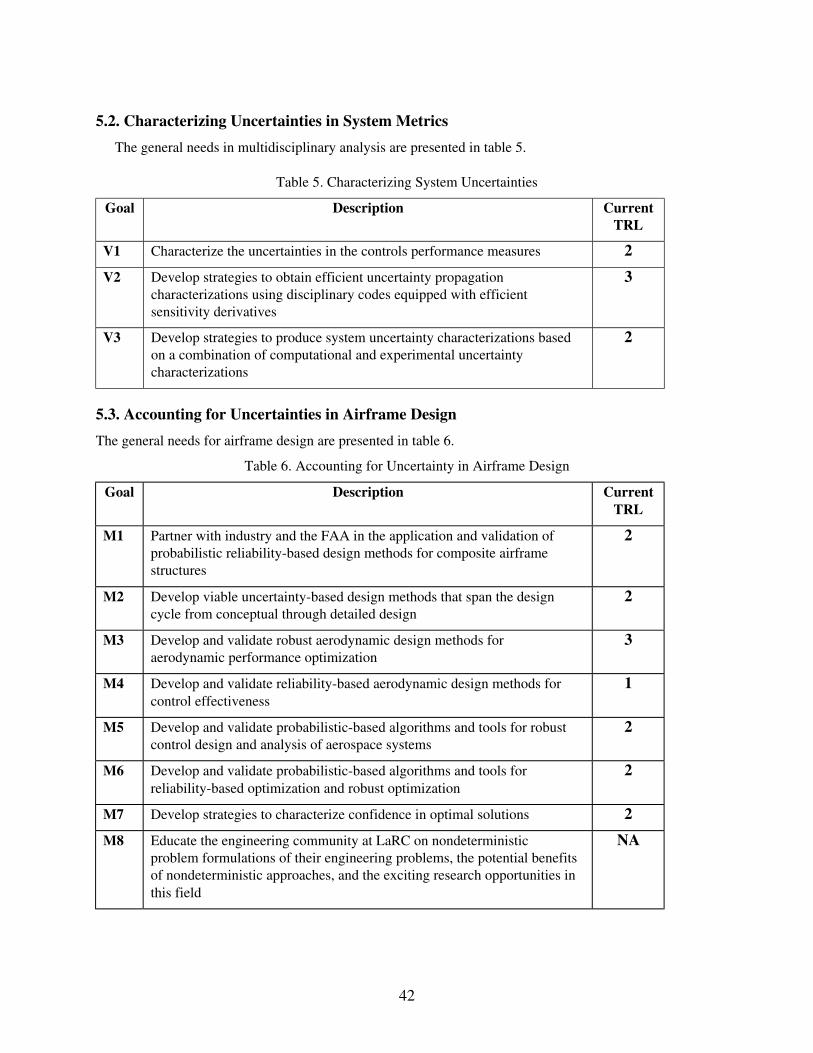
42

5.2. Characterizing Uncertainties in System Metrics

The general needs in multidisciplinary analysis are presented in table 5.

Table 5. Characterizing System Uncertainties

Goal Description CurrentTRL

V1 Characterize the uncertainties in the controls performance measures 2

V2 Develop strategies to obtain efficient uncertainty propagationcharacterizations using disciplinary codes equipped with efficientsensitivity derivatives

3

V3 Develop strategies to produce system uncertainty characterizations basedon a combination of computational and experimental uncertaintycharacterizations

2

5.3. Accounting for Uncertainties in Airframe Design

The general needs for airframe design are presented in table 6.

Table 6. Accounting for Uncertainty in Airframe Design

Goal Description CurrentTRL

M1 Partner with industry and the FAA in the application and validation ofprobabilistic reliability-based design methods for composite airframestructures

2

M2 Develop viable uncertainty-based design methods that span the designcycle from conceptual through detailed design

2

M3 Develop and validate robust aerodynamic design methods foraerodynamic performance optimization

3

M4 Develop and validate reliability-based aerodynamic design methods forcontrol effectiveness

1

M5 Develop and validate probabilistic-based algorithms and tools for robustcontrol design and analysis of aerospace systems

2

M6 Develop and validate probabilistic-based algorithms and tools forreliability-based optimization and robust optimization

2

M7 Develop strategies to characterize confidence in optimal solutions 2

M8 Educate the engineering community at LaRC on nondeterministicproblem formulations of their engineering problems, the potential benefitsof nondeterministic approaches, and the exciting research opportunities inthis field

NA

43

5.4. Approach

The approach to meet the listed needs will depend on the maturity of uncertainty-based designtechnology in the various disciplines. Early studies may be exploratory, pathfinding studies that explainprocedures and indicate possible benefits of RBD. These early studies may not involve complexmathematical models. Later studies will involve realistic mathematical models and high-fidelity analysesfor single disciplines—then multiple disciplines. These later studies will include strategies forincorporating high-performance computing.

6. Conclusions

6.1. Expected Results

The expected concrete results from a 5-year uncertainty-based design research activity are shown intable 7. In addition to providing a short goal statement with the expected output and outcome, we alsofurnish our estimate of the Research and Development Degree of Difficulty (R&D3) using the scaledeveloped by Mankins (1998):

• R&D3 – Level I: A very low degree of difficulty is anticipated in achieving R&D objectives for thistechnology. Probability of success in normal R&D effort—99 percent

• R&D3 – Level II: A moderate degree of difficulty should be anticipated in achieving R&Dobjectives for this technology. Probability of success in normal R&D effort—90 percent

• R&D3 – Level III: A high degree of difficulty anticipated in achieving R&D objectives for thistechnology. Probability of success in normal R&D effort—80 percent

• R&D3 – Level IV: A very high degree of difficulty anticipated in achieving R&D objectives for thistechnology. Probability of success in normal R&D effort—50 percent

• R&D3 – Level V: The degree of difficulty anticipated in achieving R&D objectives for thistechnology is so high that a fundamental breakthrough is required. Probability of success in normalR&D effort—20 percent

An expected intangible outcome of the concrete results of this activity will be the conversion of dozens ofother LaRC engineers to nondeterministic approaches to airframe design.

We also expect substantial interim benefits such as

1. New, inexpensive strategies for quantifying and controlling computational and experimentaluncertainties in the disciplines.

2. New, less-expensive strategies for verifying and validating computational codes and solutions.

3. Significant insight into the process of Measuring Predictive Capability.

a. What is it?

b. How do we carry it out in the face of severe nonlinearities and inference domainsseparated by different physics?

44

6.2. Opportunities for LaRC

LaRC has a window of opportunity to be in the vanguard of uncertainty-based methods formultidisciplinary airframe design. Momentum is gathering in the engineering community for thistechnological leap. LaRC has tremendous advantages in this nascent field, and can facilitate the adoptionof uncertainty-based methods by industry and NASA programs.

Table 7. Expected Results from Uncertainty-Based Design Research

Goal Output OutcomeR&D3

Level

Affordableprobabilisticanalyses

Augment high-fidelity structuresand aerodynamics tools withefficient probabilistic output

Codes provide estimates of mean andstandard deviation and/or probabilityof failure

II

Possibilisticuncertaintyquantification

Develop fundamental possibilisticstrategies and algorithms formultidisciplinary uncertaintyquantification

Reduces system risk by enablinguncertainty quantification and designfor uncertainty strategies at theconceptual design stage

IV

Aerodynamicsuncertaintyquantification

Develop efficient uncertaintyquantification and controlstrategies and algorithms foraerodynamics performance, loads,and stability and controlpredictions

Increases design confidence andaircraft safety by measuring andcontrolling uncertainty inaerodynamics performance predictionsand by enabling reliability-basedstructural design, stochastic controldesign, and reliability-basedaerodynamic controllability analysis

III

Robustaerodynamicoptimization

Develop 3-D, aerodynamic shapeoptimization algorithms thatprovide designs which are robustwith respect to uncertainties ingeometry, operating conditions,and CFD code accuracy

Controls and reduces risk by providingdesigns with aerodynamic performancethat is insensitive to intrinsicallyuncertain quantities

III

Reliability-basedstructural design

Extend CSM and experimentallyverify to predict probability offailure for composite structures

Airframe components designed withconsistent levels of reliability

IV

Probabilisticcontrols analysisand design

Develop MIMO designs that useprobabilistic input data

Safer and less conservative activecontrol of aircraft

III

Multidisciplinaryuncertainty-baseddesign

Demonstrate multidisciplinaryuncertainty-based airframe designincorporating the aerodynamics,structures and controls disciplines

Increases design confidence, controlsand reduces design risk, and increasesaircraft safety by enablinginterdisciplinary design trade-offs thatexplicitly account for uncertainty, risk,and safety

V

45

References

Abumeri, G.; and Chamis, C. 2000: Non-Deterministic Multidisciplinary Optimization of Engine Structures. AIAA-2000-4926.

Abumeri, G.; Kuguoglu, L.; and Chamis, C. 2000: Non-Deterministic Optimization—Composite Laminates, Beamsand Blades. AIAA-2000-1565.

Aeschliman, D. P.; and Oberkampf, W. L. 1998: Experimental Methodology for Computational Fluid DynamicsCode Validation. AIAA J., vol. 36, no. 5, pp. 733–742.

AGARD 1994: A Selection of Experimental Test Cases for the Validation of CFD Codes—Volume 1. AGARD-AR-303.

Alexandrov, N. M. 2001: Multilevel Methods for Optimal Design. Encyclopedia of Optimization, Volume 3, C. A.Floudas and P. M. Pardalos, eds., Kluwer, pp. 528–537.

Alexandrov, N. M.; and Lewis, R. M. 2000: Analytical and Computational Properties of Distributed Approaches toMDO. AIAA-2000-4718.

Alvin, K. F.; Oberkampf, W. L.; Rutherford, B. M.; and Diegert, K. V. 2000: Method for Characterizing Modelingand Discretization Uncertainties in Computational Simulation. SAND-2000-0515, Sandia Natl. Lab.

Anon. 1995: Assessment of Wind Tunnel Data Uncertainty. AIAA Standard S-071-1995.

Anon. 1997: Polymer Matrix Composites—Volume 3: Materials Usage, Design, and Analysis. MIL-HDBK-17-3E,U. S. Dept. of Defense. (Supersedes MIL-HDBK-17-3D, 1994.)

Apkarian, P.; and Adams, R. J. 1998: Advanced Gain-Scheduling Techniques for Uncertain Systems. IEEE Trans.Control Syst. Technol., vol. 6, no. 1, pp. 21–32.

Arbocz, J.; Starnes, J. H., Jr.; and Nemeth, M. P. 2000: A Comparison of Probabilistic and Lower Bound Methodsfor Predicting the Response of Buckling Sensitive Structures. AIAA-2000-1382.

Archetti, F.; Gaivoronski, A.; and Stella, F. 1997: Stochastic Optimization on Bayesian Nets. Eur. J. Oper. Res.,vol. 101, no. 2, pp. 360−373.

Balas, G. J.; and Doyle, J. C. 1994: Robustness and Performance Trade-Offs in Control Design for FlexibleStructures. IEEE Trans. Control Syst. Technol., vol. 2, no. 4, pp. 352–361.

Balas, G. J.; and Packard, A. K. 1996: The Structured Singular Value (Mu) Framework. CRC Controls Handbook,CRC Press, Sec. 2.3.6.

Balas, G. J.; Packard, A. K.; McCloskey, R. T.; Renfrow, J.; and Mullaney, C. 1998: Design of a Controller for theF-14 Aircraft Lateral-Directional Axis During Powered Approach. J. Guid., Control, & Dyn., vol. 21, no. 6, pp.899–908.

Barber, T. J.; Chiappetta, L. M.; DeBonis, J. R.; Georgiadis, N. J.; and Yoder, D. A. 1998: Assessment ofParameters Influencing the Prediction of Shear-Layer Mixing. J. Propuls. & Power, vol. 15, no. 1, pp. 45–53.

Beck, M. B. 1987: Water Quality Modeling: A Review of the Analysis of Uncertainty. Water Resour. Res., vol. 23,no. 8, pp. 1436–1442.

46

Belter, D. L. 1996: Application of Uncertainty Methodology at the Boeing Aerodynamics Laboratory. AIAA-96-2215.

Bendotti, P.; and Beck, C. L. 1999: On the Role of LFT Model Reduction Methods in Robust Controller Synthesisfor a Pressurized Water Reactor. IEEE Trans. Control Syst. Technol., vol. 7, no. 2, pp. 248–257.

Bode, H. W. 1945: Network Analysis and Feedback Amplifier Design. Van Nostrand.

Booker, A. J.; Dennis, J. E.; Frank, P. D.; Serafini, D. B.; Torczon, V.; and Trosset, M. W. 1998: A RigorousFramework for Optimization of Expensive Functions by Surrogates. NASA/CR-1998-208735.

Box, G. E. P.; and Draper, N. R. 1987: Empirical Model-Building and Response Surfaces. John Wiley & Sons.

Bussoletti, J. E. 1994: CFD Calibration and Validation: The Challenges of Correlating Computational ModelResults with Test Data. AIAA-94-2542.

Cahill, D. M. 1996: Application of Uncertainty Methodology for the Wind Tunnel Facilities at AEDC. AIAA-96-2216.

Campolongo, F.; Saltelli, A.; Sorensen, T.; and Tarantola, S. 2000: Hitchhiker’s Guide to Sensitivity Analysis.Sensitivity Analysis, A. Saltelli, K. Chan, and E. M. Scott, eds., John Wiley & Sons, pp. 15–47.

Chamis, C. C.; and Murthy, P. L. N. 1991: Probabilistic Composite Analysis. First NASA Advanced CompositesTechnology Conference, Part 2, NASA CP-3104-PT-2, pp. 891–900.

Chen, S.; Nikolaidis, E.; Cudney, H.; Rosca, R.; and Haftka, R. 1999: Comparison of Probabilistic and Fuzzy SetMethods for Designing Under Uncertainty. AIAA-99-1579.

Cheng Y.; and De Moor, B. L. R. 1994: Robustness Analysis and Control System Design for a Hydraulic ServoSystem. IEEE Trans. Control Syst. Technol., vol. 2, no. 3, pp. 183–197.

Choi, K. K.; and Youn, B. D. 2001: Hybrid Analysis Method for Reliability-Based Design Optimization. ASMEDesign Automation Conference, Paper No. DAC21044.

Coleman, H. W.; and Stern, F. 1997: Uncertainties and CFD Code Validation. J. Fluids Eng., vol. 119, no. 12, pp.795–803.

Cosner, R. R. 1994: Issues in Aerospace Application of CFD Analysis. AIAA-94-0464.

Cosner, R. R. 1995: CFD Validation Requirements for Technology Transition. AIAA-95-2227.

Cosner, R. R. 2000: Assessment of Vehicle Performance Predictions Using CFD. AIAA-2000-0384.

Cruse, T. A. 2001: Non-Deterministic, Non-Traditional Methods (NDNTM), NASA CR-2001-210976.

Darlington, J.; Pantelides, C.; Rustem, B.; and Tanyi, B. 1999: An Algorithm for Constrained NonlinearOptimization Under Uncertainty. Automatica, vol. 35, pp. 217−228.

DeLaurentis, D.; and Mavris, D. 2000: Uncertainty Modeling and Management in Multidisciplinary Analysis andSynthesis. AIAA-2000-0422.

Dexter, A. L. 1995: Fuzzy Model Based Fault Diagnosis, Control Theory and Applications. IEEE Proc., vol. 142,no. 6, pp. 545–550.

47

Doyle, J. 1982: Analysis of Feedback Systems with Structured Uncertainty. IEEE Proc., vol. 129D, pp. 242–250.

Doyle, J. 1983: Synthesis of Robust Controllers and Filters. IEEE Conference on Decision and Control, IEEE Press,pp. 214–220.

Doyle, J.; Wall, J.; and Stein, G. 1982: Performance and Robustness Analysis for Structured Uncertainty. IEEEConference on Decision and Control, IEEE Press, pp. 629–636.

Draper, D. 1995: Assessment and Propagation of Model Uncertainty. J. R. Stat. Soc. B, vol. 57, no. 1, pp. 45–97.

Du, X.; and Chen, W. 2000a: A Most Probable Point-Based Method for Efficient Uncertainty Analysis. ASMEDesign Automation Conference, Paper No. DAC14263.

Du, X.; and Chen, W. 2000b: Methodology for Managing the Effect of Uncertainty in Simulation-Based Design.AIAA J., vol. 38, no. 8, pp. 1471–1478.

Easterling, R. G. 2001: Measuring the Predictive Capability of Computational Models: Principles and Methods,Issues and Illustrations. SAND2001-0234, Sandia Natl. Lab.

Eisenhart, C. 1969: Realistic Evaluation of the Precision and Accuracy of Instrument Calibration Systems. PrecisionMeasurement and Calibration—Statistical Concepts and Procedures, SP 300–Vol. 1, Natl. Bur. Stand., pp.21–47.

Elsholz, E. 1997: The DLR-F4 Wing/Body Configuration. ECARP—European Computational AerodynamicsResearch Project: Validation of CFD Codes and Assessment of Turbulence Models, W. Haase, E. Chaput, E.Elsholz, M. A. Leschziner, and U. R. Muller, eds., Numerical Fluid Mechanics, pp. 429–450.

Evans, W. R. 1948: Graphical Analysis of Control Systems. Trans. AIEE, vol. 67, pp. 547–551.

Fadale, T.; and Sues, R. H. 1999: Reliability-Based Analysis and Optimal Design of an Integral Airframe StructureLap Joint. AIAA-99-1604.

Field, R. V.; Paez, T. L.; and Red-Horse, J. R. 1999: Utilizing Gauss-Hermite Quadrature to Evaluate Uncertainty inDynamic System Response. SAND98-2569C, Sandia Natl. Lab.

Frangopol, D. M.; and Iizuka, M. 1992: Probability-Based Structural System Design Using MulticriteriaOptimization. AIAA-92-4788.

Gagnon, E.; Pomerleau, A.; and Desbiens, A. 1999: Mu-Synthesis of Robust Decentralized PI Controllers. IEEEProc. Control Theory & Appl., vol. 146, no. 4, pp. 289–294.

Georgiadis, N. J.; Yoder, D. A.; and DeBonis, J. R. 1999: A Comparison of Three Navier-Stokes Solvers forExhaust Nozzle Flowfields. AIAA-99-0748.

Ghanem, R. G. 1999: Ingredients for a General Purpose Stochastic Finite Element Formulation. Comput. MethodsAppl. Mech. Eng., vol. 168, pp. 19–34.

Ghanem, R. G.; and Spanos, P. 1991: Stochastic Finite Elements: A Spectral Approach. Springer-Verlag.

Giesing, J.; and Barthelemy, J.-F. M. 1998: Summary of Industry MDO Applications and Needs. AIAA-98-4737.

Giles, M. B.; and Pierce, N. A. 1999: Improved Lift and Drag Estimates Using Adjoint Euler Equations. AIAA-99-3293.

48

Grandhi, R.; and Wang, L. 1999: Structural Reliability Analysis and Optimization: Use of Approximations.NASA/CR-1999-209154.

Grooteman, F. P. 1999: Advanced Stochastic Method of Probabilistic Analysis. NLR-TP-99398.

Habashi, W. G.; Dompierre, J.; Bourgault, Y.; Fortin, M.; and Vallet, M.-G. 1998: Certifiable Computational FluidDynamics Through Mesh Optimization. AIAA J., vol. 36, no. 5, pp. 703–711.

Ham, C.; Qu, Z.; and Johnson, R. 2000: Robust Fuzzy Control for Robot Manipulators. IEEE Proc. Control Theory& Appl., vol. 147, no. 2, pp. 212–216.

Harris, C. J.; Moore, C. G.; and Brown, M. 1993: Intelligent Control: Aspects of Fuzzy Logic and Neural Networks.World Scientific.

Hemsch, M.; Grubb, J.; Krieger, W.; and Cler, D. 2000: Langley Wind Tunnel Data Quality Assurance— CheckStandard Results. AIAA-2000-2201.

Hilburger, M. W.; and Starnes, J. H., Jr. 2000: Effects of Imperfections on the Buckling Response of Compression-Loaded Composite Shells. AIAA-2000-1387.

Holmes, M.; and Ray, A. 2001: Fuzzy Damage-Mitigating Control of a Fossil Power Plant. IEEE Trans. ControlSyst. Technol., vol. 9, no. 1, pp. 140–147.

Hung, J. Y. 1995: Magnetic Bearing Control Using Fuzzy Logic. IEEE Trans. Ind. Appl., vol. 31, no. 6, pp.1492–1497.

Huyse, L. 2001: Solving Problems of Optimization Under Uncertainty as Statistical Decision Problems. AIAA-2001-1519.

Huyse, L.; and Lewis, R. M. 2001: Aerodynamic Shape Optimization of Two-Dimensional Airfoils Under UncertainConditions. NASA/CR-2001-210648.

Inoue, K.; and Nakaoka, M. 1998: Autotuning Gain Parameter Implementation with Fuzzy Learning ControlScheme for DC Brushless Servo System. IEEE Proc. Control Theory & Appl., vol. 145, no. 5, pp. 419–427.

Isermann, R. 1998: On Fuzzy Logic Applications for Automatic Control, Supervision, and Fault Diagnosis. IEEETrans. Syst., Man, & Cybern., Part A, vol. 28, no. 2, pp. 221–235.

Jaulin, L.; and Walter, E. 1997: Global Numerical Approach to Nonlinear Discrete-Time Control. IEEE Trans.Autom. Control, vol. 42, no. 6, pp. 872–875.

Kammeyer, M. E.; and Rueger, M. L. 2000: On the Classification of Errors—Systematic, Random, and ReplicationLevel. AIAA-2000-2203.

Kowal, M.; and Mahadevan, S. 1998: Uncertainty-Based Multidisciplinary Optimization. AIAA-98-4915.

Langley, R. S. 2000: Unified Approach to Probabilistic and Possibilistic Analysis of Uncertain Systems. J. Eng.Mech., vol. 126, no. 11, pp. 1163–1172.

Lee, C. C. 1990: Fuzzy Logic in Control Systems: Fuzzy Logic Controller. IEEE Trans. Syst., Man, & Cybern., vol.20, no. 2, pp. 404–418.

Lee, K.-H.; Eom, I.-S.; Park, G.-J.; and Lee, W.-I. 1996: Robust Design for Unconstrained Optimization ProblemsUsing the Taguchi Method. AIAA J., vol. 34, no. 5, pp. 1059−1063.

49

Lim, C. M.; and Hiyama, T. 1991: Application of Fuzzy Logic Control to a Manipulator. IEEE Trans. Robot. &Autom., vol. 7, no. 5, pp. 688–691.

Lim, K. B.; and Junkins, J. L. 1987: Probability of Stability: New Measures of Stability Robustness for LinearDynamical Systems. J. Astronaut. Sci., vol. 35, no. 4, pp. 383–397.

Mankins, J. C. 1998: Research and Development Degree of Difficulty (R&D3): A White Paper. NASA internal

document.

Mayo, D. G. 1996: Error and the Growth of Experimental Knowledge. Univ. of Chicago Press.

McKay, M. D.; Beckman, R. J.; and Conover, W. J. 1979: A Comparison of Three Methods of Selecting Values ofInput Variables in the Analysis of Output from a Computer Code. Technometrics, vol. 21, pp. 239–245.

Mehta, U. 1998: Credible Computational Fluid Dynamics Simulations. AIAA J., vol. 36, no. 5, pp. 665–667.

Melchers, R. E. 1999: Structural Reliability, Analysis, and Prediction. John Wiley & Sons.

Messac, A.; and Sundararaj, G. 2000: A Robust Design Approach Using Physical Programming. AIAA-2000-0562.

Meyn, L. A. 1998: A New Method for Integrating Uncertainty Analysis Into Data Reduction Software. AIAA-98-0632.

Moser, A. N. 1993: Designing Controllers for Flexible Structures with H-Infinity/Mu-Synthesis. IEEE Cont. Syst.Mag., vol. 13, no. 2, pp. 79–89.

Muller, G. E.; and Schmid, C. J. 1978: Factor of Safety—USAF Design Practice. AFFDL-TR-78-8, U.S. Air Force.

Nair, V. N. 1992: Taguchi's Parameter Design: A Panel Discussion. Technometrics, vol. 34, pp. 127−161.

Nishimura, H.; and Kojima, A. 1999: Seismic Isolation Control for a Building-Like Structure. IEEE Control Syst.Mag., vol. 19, no. 6, pp. 38–44.

Noor, A. K.; Starnes, J. H., Jr.; and Peters, J. M. 2000: Uncertainty Analysis of Composite Structures. Comput.Methods Appl. Mech. Eng., vol. 185, pp. 413–432.

Nyquist, H. 1932: Regeneration Theory. Bell Syst. Tech. J., vol. 11, pp. 126–147.

Oberkampf, W. L. 1998: Bibliography for Verification and Validation in Computational Simulation, SAND98-2041,Sandia Natl. Lab.

Oberkampf, W. L.; and Blottner, F. G. 1998: Issues in Computational Fluid Dynamics Code Verification andValidation. AIAA J., vol. 36, no. 5, pp. 687–695.

Oberkampf, W. L.; Diegert, K. V.; Alvin, K. F.; and Rutherford, B. M. 1998: Variability, Uncertainty, and Error inComputational Simulation. AIAA/ASME Joint Thermophysics and Heat Transfer Conference, ASME-HTD-Vol.357-2, pp. 259–272.

Oberkampf, W. L.; Helton, J. C.; and Sentz, K. 2001: Mathematical Representation of Uncertainty. AIAA-2001-1645.

Oberkampf, W. L.; and Trucano, T. G. 2000: Validation Methodology in Computational Fluid Dynamics. AIAA-2000-2549.

50

Oppenheimer, E. P.; and Michel, A. N. 1988: Application of Interval Analysis Techniques to Linear Systems: I.Fundamental Results. IEEE Trans. Circuits & Syst., vol. 35, no. 9, pp. 1129–1138.

Pannu, S.; Kazerooni, H.; Becker, G.; and Packard, A. 1996: Mu-Synthesis Control for a Walking Robot. IEEEControl Syst. Mag., vol. 16, no. 1, pp. 20–25.

Patera, A. 1997: Shape Optimization by Bayesian-Validated Computer Simulation Surrogates.NASA/CR−97−206508.

Patera, A. T.; and Rönquist, E. M. 2001: A General Output Bound Result: Application to Discretization and IterationError Estimation and Control. Math. Models & Methods Appl. Sci., vol. 11, no. 4, pp. 685–712.

Piazzi, A.; and Visioli, A. 2000: Global Minimum-Jerk Trajectory Planning of Robot Manipulators. IEEE Trans.Ind. Electron., vol. 47, no. 1, pp. 140–149.

Qiu, Z. P.; Chen, H.; and Elishakoff, I. 1995: Natural Frequencies of Structures With Uncertain but NonrandomParameters. J. Optim. Theory & Appl., vol. 86, no. 3, pp. 669–683.

Rackwitz, R. 2000: Reliability Analysis—Past, Present and Future. 8th ASCE Specialty Conference on ProbabilisticMechanics and Structural Reliability, PMC2000-RRR.

Raj, P. 1998: Aircraft Design in the 21st Century: Implications for Design Methods. AIAA-98-2895.

Raj, P.; and Singer, S. W. 1991: Computational Aerodynamics in Aircraft Design: Challenges and Opportunities forEuler/Navier-Stokes Methods. IPAC Paper No. 911990.

Rao, S. S.; and Berke, L. 1997: Analysis of Uncertain Structural Systems Using Interval Analysis. AIAA J., vol. 35,no. 4, pp. 727–735.

Rizzi, A.; and Vos, J. 1998: Toward Establishing Credibility in Computational Fluid Dynamics Simulations. AIAAJ., vol. 36, no. 5, pp. 668–675.

Roache, P. J. 1990: Need for Control of Numerical Accuracy. J. Spacecr., vol. 27, no. 2, pp. 98–102.

Roache, P. J. 1998: Verification and Validation in Computational Science and Engineering. Hermosa Publ.

Roberts, T. W.; Sidilkover, D.; and Thomas, J. L. 2000: Multigrid Relaxation of a Factorizable, ConservativeDiscretization of the Compressible Flow Equations. AIAA-2000-2252.

Robinson, D. G. 1998: Survey of Probabilistic Methods Used in Reliability, Risk, and Uncertainty Analysis:Analytical Techniques. SAND-98-1189, Sandia Natl. Lab.

Rogallo, R. S.; and Moin, P. 1984: Numerical Simulation of Turbulent Flows. Annu. Rev. Fluid Mech., vol. 16, pp.99–137.

Romero, V. J. 1999: Efficient Global Optimization Under Conditions of Noise and Uncertainty: A Multi-ModelMulti-Grid Windowing Approach. Proceedings of the 3rd World Congress of Structural and MultidisciplinaryOptimization, UBCAD/ISSMO, pp. 40–46.

Romero, V. J.; Eldred, M. S.; Bonhoff, W. J.; and Outka, D. E. 1995: Application of Optimization to the InverseProblem of Finding the Worst-Case Heating Configuration in a Fire. Numerical Methods in Thermal Problems,vol. 9, part 2, R. W. Lewis and P. Durbetaki, eds., Pineridge Press, Swansea, U.K., pp. 1022–1033. (Alsoavailable as SAND95-1364C, Sandia Natl. Lab.)

51

Roy, R. K. 1990: A Primer on the Taguchi Method. Society of Manufacturing Engineers.

Rubbert, P. E. 1990: The Impact of Supercomputers on CFD. Comput. Syst. Eng., vol. 1, no. 1, pp. 1–6.

Rubbert, P. E. 1994: CFD and the Changing World of Airplane Design. ICASE-94-0.2.

Rubbert, P. E. 1998: On Replacing the Concept of CFD Validation with Uncertainty Management. Presented atFourth World Conference in Applied Fluid Dynamics: World Fluid Dynamics Days 1998—Validation, Qualityand Reliability.

Rubbert, P. R.; and Goldhammer, M. 1989: CFD in Design: An Airframe Perspective. AIAA-89-0092.

Safonov, M. G. 1977: Robustness and Stability Aspects of Stochastic Multi-Variable Feedback Design. Ph.D.Dissertation, Massachusetts Institute of Technology.

Saltelli, A.; Chan, K.; and Scott, E. M., eds. 2000: Sensitivity Analysis. John Wiley & Sons.

Scherer, C.; Gahinet, P.; and Chilali, M. 1997: Multiobjective Output-Feedback Control via LMI Optimization.IEEE Trans. Autom. Control, vol. 42, no. 7, pp. 896–911.

Spencer, B. F. 1994: Reliability-Based Measures of Structural Control Robustness. Struct. Saf., vol. 15, pp.111–129.

Spencer, B. F.; Sain, M. K.; Kantor, J. C.; and Montemagno, C. 1992: Probabilistic Stability Measures forControlled Structures Subject to Real Parameter Uncertainties. Smart Mater. & Struct., vol. 1, pp. 294–305.

Stengel, R. F. 1980: Some Effects of Parameter Variations on the Lateral-Directional Stability of Aircraft. J. Guid.& Control, vol. 3, no. 2, pp. 124–131.

Stengel, R. F. 1991: Stochastic Robustness of Linear Time-Invariant Control Systems. IEEE Trans. Autom. Control,vol. 36, no. 1, pp. 82–87.

Stroud, W. J.; Krishnamurthy, T.; and Smith, S. A. 2001: Probabilistic and Possibilistic Analyses of the Strength ofa Bonded Joints. AIAA-2001-1238.

Sundararajan, C., ed. 1995: Probabilistic Structural Mechanics Handbook, Theory and Industrial Applications.Chapman & Hall.

Tada, Y.; Matsumoto, R.; and Yoshida, M. 1988: Reliability-Based Optimum Design of Continuum Structures.JSME Int. J., vol. 31, Oct., pp. 690−696.

Taguchi, G. 1987: System of Experimental Design: Engineering Methods to Optimize Quality and Minimize Cost.UNIPUB.

Taylor, A. C. 2000: Aerodynamic Uncertainty Studies. NASA/CR-2000-210327.

Teng, A.; Free, J.; and Parkinson, A. 1992: An Approach to Robust Design of Dynamic Systems—Allocation ofVariation. AIAA-92-4790.

Thacker, B. H.; Riha, D. S.; Millwater, H. R.; and Enright, M. P. 2001: Errors and Uncertainties in ProbabilisticEngineering Analysis. AIAA-2001-1239.

Torczon, V.; and Trosset, M. 1998: Using Approximations to Accelerate Engineering Design Optimization. AIAA-98-4800.

52

Torng, T. Y.; Funk, G. E.; and Stephenson, R. M. 1999: Probabilistic On-Orbit Loads Combination Assessment.AIAA-99-1576.

Torng, T. Y.; and Yang, R. J. 1994: A Reliability-Based Design Optimization Procedure for Minimal Variations.AIAA-94-1415.

Ugur Koyluoglu, H.; and Elishakoff, I. 1998: A Comparison of Stochastic and Interval Finite Elements Applied toShear Frames With Uncertain Stiffness Properties. Comput. & Struct., vol. 67, no. 3, pp. 91–98.

Unal, R.; Stanley, D.; and Joyner, C. R. 1993: Propulsion System Design Optimization Using the Taguchi Method.IEEE Trans. Eng. Manage., vol. 40, no. 3, pp. 315−322.

Venditti, D. A.; and Darmofal, D. L. 2000: Adjoint Error Estimation and Grid Adaptation for Functional Outputs:Application to Quasi-One-Dimensional Flow. J. Comput. Phys., vol. 164, no. 1, pp. 204–227.

Venter, G.; and Haftka, R. T. 1999: Using Response Surface Approximations in Fuzzy Set Based DesignOptimization. Struct. Optim., vol. 18, no. 4, pp. 218–227.

Waggoner, E. G.; Burt, M.; Lekoudis, S.; Kaynak, U.; Hirschel, E. H.; and Korner, H. 1994: CFD Requirements forCode Validation. A Selection of Experimental Test Cases for the Validation of CFD Codes—Vol. 1, AGARD AR-303.

Weingarten, V. I.; and Seide, P. 1968: Buckling of Thin-Walled Truncated Cones. NASA SP-8019.

Weingarten, V. I.; Seide, P.; and Peterson, J. P. 1968: Buckling of Thin-Walled Circular Cylinders. NASA SP-8007.

Weingarten, V. I.; and Seide, P. 1969: Buckling of Thin-Walled Doubly Curved Shells. NASA SP-8032.

Wheeler, D. J. 1990: Understanding Industrial Experimentation. SPC Press.

Wheeler, D. J.; and Chambers, D. S. 1992: Understanding Statistical Process Control. Second Ed., SPC Press.

Wiener, N. 1938: The Homogeneous Chaos. American J. Math., vol. 60, pp. 897–936.

Wu, Y.-T.; and Wirsching, P. H. 1989: New Algorithm for Structural Reliability Estimation. ASCE J. Eng. Mech.,vol. 113, pp. 1319–1334.

Xiu, D.; and Karniadakis, G. E. 2001: The Wiener-Askey Polynomial Chaos for Stochastic Differential Equations.Center for Fluid Mechanics Rep. 01-1, Brown University.

Yoon, S.-B.; Jung, I.-S.; and Hyun, D.-S. 1999: Robust Shape Optimization of Electromechanical Devices. IEEETrans. Magn., vol. 35, no. 3, pp. 1710–1713.

Young, J.; Anderson, R.; and Yurkovich, R. 1998: A Description of the F/A-18E/F Design and Design Process.AIAA-98-4701.

53

Appendix A.

Technology Readiness Levels

The Technology Readiness Levels (TRLs) are defined as follows:

TRL 9: Actual system “mission proven” through successful mission operations. Thoroughlydebugged software readily repeatable. Fully integrated with operational hardware/software systems. Alldocumentation completed. Successful operational experience. Sustaining software engineering support inplace. Actual system fully demonstrated.

TRL 8: Actual system completed and “mission qualified” through test and demonstrationin an operational environment. Thoroughly debugged software. Fully integrated with operationalhardware and software systems. Most user documentation, training documentation, and maintenancedocumentation completed. All functionality tested in simulated and operational scenarios. Verificationand validation completed.

TRL 7: System prototype demonstration in high-fidelity environment (parallel or shadowmode operation). Most functionality available for demonstration and test. Well integrated withoperational hardware/software systems. Most software bugs removed. Limited documentation available.

TRL 6: System/subsystem prototype demonstration in a relevant end-to-end environment.Prototype implementations on full-scale realistic problems. Partially integrated with existinghardware/software systems. Limited documentation available. Engineering feasibility fully demonstrated.

TRL 5: Module and/or subsystem validation in relevant environment. Prototypeimplementations conform to target environment/interfaces. Experiments with realistic problems.Simulated interfaces to existing systems.

TRL 4: Module and/or subsystem validation in laboratory environment. Stand-aloneprototype implementations. Experiments with full-scale problems or data sets.

TRL 3: Analytical and experimental critical function and/or characteristic proof-of-concept. Limited functionality implementations. Experiments with small representative data sets.Scientific feasibility fully demonstrated.

TRL 2: Technology concept and/or application formulated. Basic principles coded. Experimentswith synthetic data. Mostly applied research.

TRL 1: Basic principles observed and reported. Basic properties of algorithms, representations,and concepts. Mathematical formulations. Mix of basic and applied research.