necessary and probably sufﬁcient test for finding...

Necessary and Probably Sufficient Test for FindingValid Instrumental VariablesAmit Sharma ∗ 1,2

1Microsoft Research, New [email protected]

ABSTRACT

Increasing availability of fine-grained data from diverse fields spanning the social and biomedical sciences presents newopportunities for gaining causal knowledge. While inferring the global causal graph or mechanisms is usually intractable, localcausal estimation methods such as instrumental variables (IV) can be used for estimating causal effects. However, IV methodsdepend on two assumptions—exclusion and as-if-random—that are largely believed to be untestable from data, thus making ithard to evaluate the validity of an instrumental variable or compare estimates across studies even on the same dataset. Inthis paper, we show that when all variables are discrete, testing for instrumental variables is possible. We build upon priorwork on necessary tests to derive a necessary and probably sufficient test for the validity of an instrumental variable. Givenobservational data on a pair of cause and effect variables, the proposed test determines whether an instrument is valid withinsome statistical error. The test works by defining the class of invalid-IV and valid-IV causal models in terms of Bayesiangraphical models and comparing their marginal likelihood based on observed data.Simulations of randomly selected causal models show that the test is most powerful for moderate-to-weak instruments;incidentally, such instruments are most commonly used in observational studies. It is also able to distinguish between invalidand valid IV causal models for an open problem proposed in past work. Applying the test to two seminal studies on instrumentalvariables and five recent studies from the American Economic Review shows that many of the instruments are flawed, at leastwhen all variables are discretized. The proposed test opens the possibility of algorithmically finding and validating instrumentsin large datasets and more generally, adopting a data-driven approach to instrumental variable studies.

1 INTRODUCTIONThe method of instrumental variables is one of the most popular ways to estimate causal effects from observational data in thesocial and biomedical sciences. The key idea is to find subsets of the data where conditions were nearly the same as they wouldin a randomized experiment, and use those subsets to estimate causal effect. For example, instrumental variables have beenused in economics to study the effect of policies such as military conscription and compulsory schooling on future earnings1, 2,and in epidemiology (under the name Mendelian randomization) to study the effect of risk factors on disease outcomes3.

Figure 1a shows the canonical causal inference problem for the instrumental variables (IV) method. The goal is to estimatethe effect of variable X on another variable Y based on observed data. However, there are unobserved (and possibly unknown)common causes for X and Y that contribute to the observed association between X and Y, making the isolation of X’s effect onY a non-trivial problem. Compared to conditioning approaches such as stratification or matching4, instrumental variables havethe advantage that they do not require observing any of the confounders to estimate the causal effect. Rather, identificationrelies on finding an additional variable Z, that acts as an instrument to modify the distribution of X , as shown by the arrowZ → X in Figure 1a.

To be a valid instrument, however, Z should satisfy three conditions2. First, Z should have a substantial effect on X . That is,Z causes X (Relevance). Second, Z should not cause Y directly (Exclusion); the only association between Z and Y should bethrough X . Third, Z should be independent of all the common causes U of X and Y (As-if-random). The latter two conditionsare shown in the graphical model in Figure 1b. Taken together, the as-if-random and exclusion conditions are equivalent toZ ⊥⊥ U and Z ⊥⊥ Y ||X,U respectively.

However, the Achilles heel of any instrumental variable analysis is that these core conditions are never tested systematically.Except for relevance (which can be tested by looking at the observed correlation between Z and X), the other conditions areusually considered as assumptions, and are defended with qualitative domain knowledge. This can be problematic, especiallybecause the entire validity of the IV estimate depends on the exclusion and as-if-random conditions. It also makes it hard tocompare and evaluate studies that use instrumental variables.

∗I acknowledge Jake Hofman and Duncan Watts for their valuable feedback throughout the course of this work.

1

(a) Valid-IV causal model (b) Invalid-IV causal model

Figure 1. Standard instrumental variable causal model and common violations that lead to an invalid-IV model. Exclusioncondition is violated when the instrumental variable Z directly affects the outcome Y . As-if-random condition is violated whenunobserved confounders U also affect the instrumental variable Z.

As a remedy, there is a line of work using causal graphical models that devises necessary tests that follow from the IVconditions5, 6. These tests can be used to weed out bad instruments, but are inconclusive whenever an instrument passes thetest. Other tests such as the Durbin-Wu-Hausman test7 are sufficient, but require knowledge of at least one valid instrumentalvariable; the circular nature of the test makes it impractical for most situations. These shortcomings have led scholars to declareinstrumental variables as untestable from data8, 9.

In this paper, we show that whenever X ,Y and Z are discrete, it is possible to test for the validity of an instrumental variableusing observational data only. By combining ideas from causal graphical models and Bayesian statistics, we present a necessaryand probably sufficient test for instrumental variables. While not provably sufficient, the proposed test quantifies the likelihoodthat an instrument is valid given the observed data sample. Specifically, it compares the probability of a valid-IV model to theprobability of an invalid-IV model, given the observed data.

Simply computing the likelihood of generating observed data from these two classes of models—valid-IV and invalid-IV—will not help because the class of invalid-IV models, as shown in Figure 1b also includes the class of valid-IV modelsby definition. Therefore, any data distribution generated by a valid-IV model can also be generated by an invalid-IV model.To devise an informative statistical test, we need some way of identifying how a data distribution generated by a valid-IVmodel differs from invalid-IV models. Here we make use of a necessary conditions for instrumental variables proposed byPearl5 that restricts the joint probability distributions for P (X,Y, Z) that any valid-IV model can generate. Armed with theseconditions, our proposed statistical test proceeds as follows. If the observed data does not satisfy the necessary conditions, thenit is declared invalid. If it does, then the relative likelihood of a valid-IV model is computed by estimating the joint likelihoodof satisfying all necessary conditions and generating the observed data.

In theory, evaluating the test depends on enumerating and testing all possible causal models—both valid and invalidinstrumental variable models—that could have generated the data. However, it is impossible to enumerate all causal modelsbecause there can be infinitely many models within the class of valid and invalid-IV models. Therefore, we introduce samplingstrategies to approximate the enumeration. For simplicity, we first present a uniform sampling strategy assuming that all causalmodels are equally likely. However, given observed data, some of the models may be more likely than others. Therefore, wealso present a computationally intensive sampling strategy that selects underlying causal models based on their likelihood ofgenerating the observed data.

Finally, any statistical test is only as good as the decisions it helps to support. Using simulations, we show that the proposedNPS test is most effective for validating instruments having a low correlation with the cause of interest. Coincidentally, most ofthe instruments used in observational studies in the social and biomedical sciences also satisfy this property. To demonstrateits usefulness, we apply the test to datasets from two seminal papers on instrumental variables. In both cases, we find thatinstrumental assumptions used in the corresponding papers were possibly flawed, at least when variables are discretized.We also apply the NPS test to validate recent instrumental variable studies in the American Economic Review, a premiereconomics journal. Looking forward, the proposed test makes it possible to compare potential instruments for their validity,allow transparent comparisons between multiple IV studies, and enable more data-driven search for natural experiments10.

2 BACKGROUND: TESTABILITY OF AN INSTRUMENTAL VARIABLESince sufficient conditions for validity of an instrument (Z ⊥⊥ U and Z ⊥⊥ Y |X,U ) depend on an unobserved variable U , thevalidity of an instrumental variable is largely believed to be untestable from observational data alone8. Nevertheless, there aresome statistical tests that can be used to examine an instrumental variable. These tests either provide necessary conditions for a

2/24

Valid−IV

Invalid−IV

(a) Data distributions generated by Valid-IVand Invalid-IV models

Valid−IV

Invalid−IV

(b) Data distributions that pass Pearl’snecessary test

Valid−IV

Invalid−IV

(c) Data distributions that pass proposed NPStest

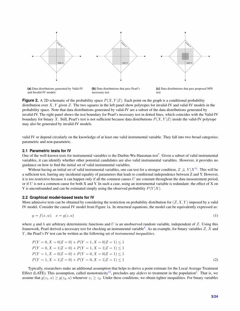
Figure 2. A 2D schematic of the probability space P (X,Y |Z). Each point on the graph is a conditional probabilitydistribution over X , Y given Z. The two squares in the left panel show polytopes for invalid-IV and valid-IV models in theprobability space. Note that data distributions generated by valid-IV are a subset of the data distributions generated byinvalid-IV. The right panel shows the test boundary for Pearl’s necessary test in dotted lines, which coincides with the Valid-IVboundary for binary X . Still, Pearl’s test is not sufficient because data distributions P (X,Y |Z) inside the valid-IV polytopemay also be generated by invalid-IV models.

valid IV or depend circularly on the knowledge of at least one valid instrumental variable. They fall into two broad categories:parametric and non-parametric.

2.1 Parametric tests for IVOne of the well-known tests for instrumental variables is the Durbin-Wu-Hausman test7. Given a subset of valid instrumentalvariables, it can identify whether other potential candidates are also valid instrumental variables. However, it provides noguidance on how to find the initial set of valid instrumental variables.

Without having an initial set of valid instrumental variables, one can test for a stronger condition, Z ⊥⊥ Y |X11. This will bea sufficient test, barring any incidental equality of parameters that leads to conditional independence between Z and Y. However,it is too restrictive because it can happen only if all the common causes U are constant throughout the data measurement period,or if U is not a common cause for both X and Y. In such a case, using an instrumental variable is redundant: the effect of X onY is unconfounded and can be estimated simply using the observed probability P (Y |X).

2.2 Graphical model-based tests for IVMore admissive tests can be obtained by considering the restriction on probability distribution for (Z,X, Y ) imposed by a validIV model. Consider the causal IV model from Figure 1a. In structural equations, the model can be equivalently expressed as:

y = f(x, u); x = g(z, u) (1)

where g and h are arbitrary deterministic functions and U is an unobserved random variable, independent of Z. Using thisframework, Pearl derived a necessary test for checking an instrumental variable5. As an example, for binary variables Z, X andY , the Pearl’s IV test can be written as the following set of instrumental inequalities.

P (Y = 0, X = 0|Z = 0) + P (Y = 1, X = 0|Z = 1) ≤ 1

P (Y = 0, X = 1|Z = 0) + P (Y = 1, X = 1|Z = 1) ≤ 1

P (Y = 1, X = 0|Z = 0) + P (Y = 0, X = 0|Z = 1) ≤ 1

P (Y = 1, X = 1|Z = 0) + P (Y = 0, X = 1|Z = 1) ≤ 1 (2)

Typically, researchers make an additional assumption that helps to derive a point estimate for the Local Average TreatmentEffect (LATE). This assumption, called monotonicity12, precludes any defiers to treatment in the population2. That is, weassume that g(z1, u) ≥ g(z2, u) whenever z1 ≥ z2. Under these conditions, we obtain tighter inequalities. For binary variables

3/24

Z, X and Y , the instrumental inequalities become:

P (Y = y,X = 1|Z = 1) ≥ P (Y = y,X = 1|Z = 0) ∀y ∈ {0, 1} (3)P (Y = y,X = 0|Z = 0) ≥ P (Y = y,X = 0|Z = 1) ∀y ∈ {0, 1} (4)

Whenever any of these inequalities are violated, it implies that one or more of the IV assumptions—exclusion, as-if-randomor monotonicity—are violated. Based on these instrumental inequalities, different hypothesis tests can been derived to accountfor sampling variability in observing the true conditional distributions. For example, a null hypothesis tests based on thechi-squared statistic13 or the Kolmogorov-Smirnov test statistic14 have been proposed.

When X , Y and Z is binary, this test is not only necessary, it is the strongest necessary test possible6, 14. In other words, ifan observed data distribution satisfies the test, then there does exist at least one valid-IV causal model that could have generatedthe data; we call this the existence property. However, it does not satisfy the existence property when all variables are notbinary, allowing probability distributions that cannot be generated by any valid-IV model. To rectify this, Bonet proposed amore general version of the test that ensures the existence property for any discrete-valued X , Y and Z.6. We call this test asthe Pearl-Bonet necessary and existence test for instrumental variables, or simply the Pearl-Bonet test.

While Bonet presented theoretical properties of the test for discrete variables, implementing the test in practice is non-trivialbecause it involves testing membership of a convex polytope in high-dimensional space. Further, the test does not support themonotonicity assumption, a popular assumption instrumental variable methods. In this paper, therefore, we extend Bonet’swork by incorporating monotonicity and present a practical method for testing IVs when variables can have arbitrary number ofdiscrete levels.

2.3 Towards a sufficient testThe above tests can refute an invalid-IV model, but are unable to verify a valid-IV model14. That is, even when an observeddata distribution passes the necessary test, it does not exclude the possibility that data was generated by an invalid-IV model.To see why, let us look at Figure 2 that shows the relationship between an observed data distribution and Valid-IV or Invalid-IVmodels. Each point in Figure2a represents a probability distribution over X , Y and Z.1 The two squares bound the probabilitydistributions that can be generated by any Valid-IV or Invalid-IV model. As can be seen from the figure, probability distributionsgeneratable from Valid-IV are a strict subset of the distributions generatable by the invalid-IV model. This implies that even if astatistical test can accurately identify the boundary for valid-IV models, as in Figure 2b, we can never be sure whether theprobability distribution was actually generated by a valid-IV or invalid-IV model.

Therefore, a harder problem is to establish sufficiency: determining whether observed data was generated by a valid IVmodel. One way to establish this is by comparing the likelihood of different causal models given the data. However, as weargued above, likelihood-based approaches for graphical models15 are not informative because invalid-IV models (as shown inFigures 1b and 2b) are more general than the valid-IV model and thus are always as likely (or more) to generate the observeddata.

In this paper, we show that comparing the Bayesian evidence between valid-IV and invalid-IV models can be used totest for the validity of an instrumental variable. Unlike past statistical tests13, 14 that refute a null hypothesis that observeddata was generated from a valid-IV model, we do so by comparing the probability of valid-IV and invalid-IV models givenobserved data. More precisely, given a probability distribution P (X,Y, Z) from observed data, the test computes the ratioof marginal likelihoods for valid and invalid IV models. Whenever this marginal likelihood ratio is above a pre-determinedacceptance threshold, our test concludes that the instrument is valid. To distinguish this statistical notion from deterministicsufficiency—conditions that would determine in absolute whether an instrument is valid or not—we call such a sufficiency asprobable sufficiency.

Probable Sufficiency for Instrumental Variables: If an observed data distribution passes Pearl’s necessary test, howlikely is it that it was generated from a valid-IV model compared to an invalid-IV model?

Intuitively, we wish to find out how often does Pearl’s necessary test provide a wrong answer. That is, how often does anobserved distribution that was generated by an invalid-IV model pass the necessary test? Once we know that, we can compute

1The axes represent the space of conditional probabilities P (X,Y |Z). We use the fact that any observed probability distribution P over X , Y and Zcan be specified by a set of conditional probabilities of the form P (X = x, Y = y|Z = z). For example, for binary variables, this would be a set of eightconditional probabilities6. The corresponding 8-dimensional real vector would be:

F (P) =(P (X = 0, Y = 0|Z = 0), P (X = 0, Y = 1|Z = 0), P (X = 1, Y = 0|Z = 0), P (X = 1, Y = 1|Z = 0),

P (X = 0, Y = 0|Z = 1), P (X = 0, Y = 1|Z = 1), P (X = 1, Y = 0|Z = 1), P (X = 1, Y = 1|Z = 1))

(5)

The 2-D squares represented in Figures 2a,b are actually polytopes in this multi-dimensional space. The extreme points for F (P), or equivalently for invalid-IVmodels are characterized by P (X = x, Y = y|Z = z) = 1 ∀z. The boundary shown for NPS test in Figure 2c is however, an oversimplification. The set ofconditional distributions (or equivalently, instruments) that can be validated by the NPS test is unknown and most likely will constitute many regions in theprobability space, instead of a single bounded region as shown.

4/24

the probability that a given observed distribution was generated by a valid-IV model, based on the result of Pearl’s necessarytest.

Combined, Pearl’s necessary test and our probable sufficiency test provide a framework for testing instrumental variables,which we call the Necessary and Probably Sufficient (NPS) test for instrumental variables. Any valid instrument needs to passPearl’s test. Therefore, NPS test provides necessity: any instrument that fails Pearl’s instrumentality inequalities is not a validinstrument. Further, NPS test provides sufficiency: any instrument that satisfies Pearl’s instrumental inequalities and passes theprobable sufficiency test can be accepted as a valid instrument. That said, NPS test will be inconclusive for some instruments:those that satisfy Pearl’s inequalities but the marginal likelihood ratio remains close to 1. Figure 2c shows these possibilities.As shown by the dark grey box in the center, NPS test validates a subset of all possible valid-IV models.

In the next two sections, we describe the NPS test formally. Section 3 presents a general Validity Ratio statistic that canbe used to compare Valid-IV and Invalid-IV models. We do so by introducing a probabilistic generative meta-model thatformalizes the connection between IV assumptions, causal models and the observed data. The key detail for computing theValidiity Ratio is in selecing a suitable sampling strategy for causal models. Section 4 describes one such strategy based on theresponse variable framework11.

For the rest of the paper, we assume that X , Y and Z are all discrete. In principle, we can apply the NPS testing frameworkto both continuous and discrete values for X , Y and Z. However, the test is expected to be most informative when X is discrete.This is because when X is continuous, the region for Valid-IV identified by Pearl’s necessary test coincides with the Invalid-IVregion and the necessary test becomes uninformative6.

For ease of exposition, we present the NPS test using binary Z, X and Y . In Section 5, we discuss how the test extends tothe case where Z, X and Y can be arbitrary discrete variables. Finally, Sections 6 and 7 demonstrate the practical applicabilityof the test using simulation data and data from past IV studies.

3 A NECESSARY AND PROBABLY SUFFICIENT (NPS) TESTThe key idea behind the NPS test is that we can compare marginal likelihoods of valid-IV and invalid-IV class of models. To doso, we first describe a Bayesian meta-model that describes how observed data can be generated from different values of theexclusion and as-if-random conditions. We then provide the main result that provides a Validity Ratio to compare valid-IV andinvalid-IV models, followed by pseudo-code for an algorithm that uses the NPS test to validate an instrumental variable.

3.1 Generating valid-IV and invalid-IV causal modelsAs mentioned above, our strategy depends on simulating all causal models—both valid-IV and invalid-IV models—that couldhave generated the observed data. Therefore, we first describe a probabilistic generative meta-model of how the observed datais generated from a causal model.

Let us first define the valid-IV and invalid-IV models formally in terms of the IV assumptions. A valid IV model doesnot contain an edge from Z → Y or from U → Z, as shown in Figure 1a. This implies that both Exclusion and As-if-random conditions hold for a valid-IV model. For our example above, this would mean an encouragement instrument thatis not confounded by common causes for peers’ activities and encouragement to an individual does not directly lead to anencouragement for her peer, except through social influence. Conversely, a causal model is an invalid IV model when at leastone of Exclusion or As-if-random conditions is violated, as shown by the dotted arrows in Figure 1b. Therefore, assuming thecausal structure Z → X → Y , there are two classes of causal models that can generate observed data distributions over X , Yand Z:

• Valid IV model: E = True and R = True

• Invalid IV model: Not (E = True and R = True)

where E denotes the exclusion restriction and R denote the as-if-random restriction.Each of these classes of causal models—valid and invalid IV—in turn contains multiple causal models, based on the specific

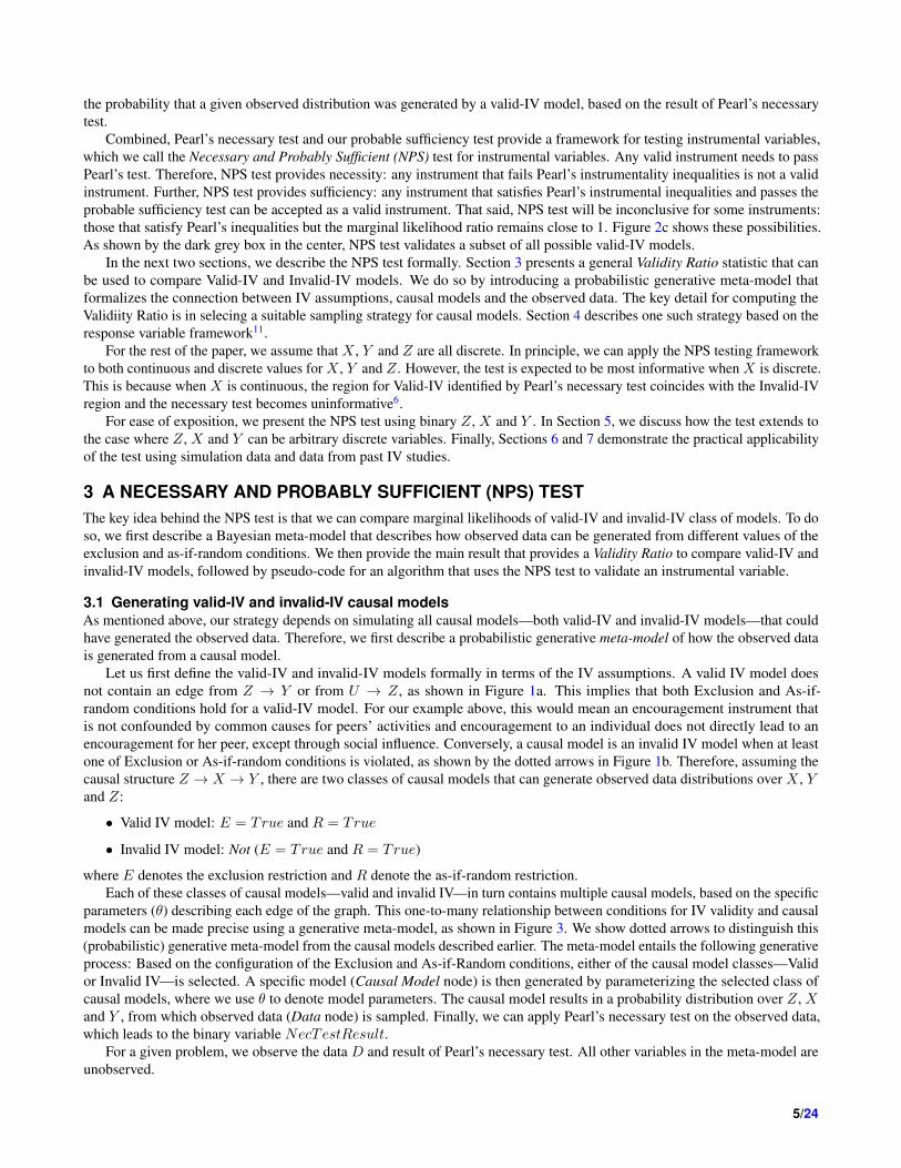
parameters (θ) describing each edge of the graph. This one-to-many relationship between conditions for IV validity and causalmodels can be made precise using a generative meta-model, as shown in Figure 3. We show dotted arrows to distinguish this(probabilistic) generative meta-model from the causal models described earlier. The meta-model entails the following generativeprocess: Based on the configuration of the Exclusion and As-if-Random conditions, either of the causal model classes—Validor Invalid IV—is selected. A specific model (Causal Model node) is then generated by parameterizing the selected class ofcausal models, where we use θ to denote model parameters. The causal model results in a probability distribution over Z, Xand Y , from which observed data (Data node) is sampled. Finally, we can apply Pearl’s necessary test on the observed data,which leads to the binary variable NecTestResult.

For a given problem, we observe the data D and result of Pearl’s necessary test. All other variables in the meta-model areunobserved.

5/24

Exclusion

Causal Model

As-if-Random θ

Data

NecTestResult

Figure 3. A probabilistic graphical meta-model for describing the connection between IV conditions and specific causalmodels. Evidence consists of both the results of the necessary test and observed data sample. Therefore, given this evidence,some causal models are expected to become more likely than others. Note that arrows are dotted to distinguish theseprobabilistic diagrams from the causal diagrams in Figure 1.

3.2 Comparing likelihood of valid-IV and invalid-IV modelsLet PT denote whether the observed data passed the necessary test. We wish to estimate whether the data was generated from aValid IV model. We can compare the likelihood of observing PT and D given that both Exclusion and As-if-random conditionsare valid, versus when they are not.

Theorem 1. Given a representative data sample D drawn from P (X,Y, Z) over variables X , Y , Z, result of Pearl’s necessarytest PT on the data sample, the validity of Z as an instrument for estimating causal effect of X on Y can be decided using thefollowing evidence ratio of valid and invalid classes of models:

Validity-Ratio =P (E,R|PT,D)

P (¬(E,R)|PT,D)=

P (PT,D|E,R) ∗ P (E,R)

P (PT,D|¬(E,R)) ∗ P (¬(E,R))(6)

=P (M1)

P (M2)

∫M1:m is valid P (m|E,R)P (D|m)dm∫

M2:m is invalid IPTm .P (m|¬(E,R))P (D|m)dm(7)

where M1 and M2 denote classes of valid-IV and invalid-IV causal models respectively. P (D|m) represents the likelihood ofthe data given a causal model m. P (m|E,R) and P (m|¬(E,R) denote the prior probability of any model m within the classof valid-IV and invalid-IV causal models respectively, and IPTm is an indicator function which is 1 whenever a causal model mgenerates a data distribution that passes the Pearl-Bonet necessary test.

This is similar to the Bayes Factor16, except that we are additionally using the result of the Pearl-Bonet necessary test tocompute evidence.

The proof of the theorem follows from the structure of the generative meta-model and properties of Pearl’s necessary test.

Proof. Let us first consider the ratio of marginal likelihoods of the two model classes.

ML-Ratio =P (PT,D|E,R)

P (PT,D|¬(E,R))(8)

Since the Pearl’s test is a necessary test, we know that P (PT |E,R) = 1. Thus, the numerator becomes:

P (PT,D|E,R)

= P (PT |D,E,R)P (D|E,R)

= P (D|E,R) (9)

6/24

Further, for any causal model m, we know with certainty whether it follows exclusion and as-if-random restrictions. Inparticular, P (minvalidIV |E,R) = 0. Using this observation, we can write the numerator of the ML-Ratio as:

P (D|E,R)

=

∫m

P (D,m|E,R)dm

=

∫m

P (m|E,R)P (D|m)dm

=

∫M1:m is valid

P (m|E,R)P (D|m)dm (10)

Similarly, the denominator can be expressed by,

P (PT,D|¬(E,R))

=

∫m

P (PT,D,m|¬(E,R))dm

=

∫m

P (m|¬(E,R))P (PT,D|m,¬(E,R))dm

=

∫M2:m is invalid

P (m|¬(E,R))P (PT,D|m)dm (11)

where we use the conditional independencies entailed by the generative meta-model. Now given a model m, the result ofPearl-Bonet necessary test PT is deterministic. Therefore, P (PT |M) is 1 whenever the data distribution P (x, y, z) generatedby a causal model m passes the test, and 0 otherwise. Assuming that D is a representative sample from data distributioninduced by each m, the denominator then simplifies to:∫

M2:m is invalidP (m|¬(E,R))P (PT,D|m)dm =

∫M2:m is invalid

P (m|¬(E,R))P (D|m)IPTmdm (12)

where IPTmis an indicator function, evaluating to 1 whenever causal model m passes the Pearl-Bonet test.

Combining Equations 10 and 12, we obtain the ratio of marginal likelihoods:

ML-Ratio =P (PT,D|E,R)

P (PT,D|¬(E,R))=


M2:m is invalid IPTm.P (m|¬(E,R))P (D|m)dm

(13)

Finally, by definition of model classes M1 and M2, they correspond to valid and invalid classes of causal models. Thus,

P (E,R)

P (¬(E,R))=P (M1)

P (M2)(14)

The above two equations lead us to the main statement of the theorem:

Validity-Ratio =P (M1)

P (M2)


M2:m is invalid IPTm .P (m|¬(E,R))P (D|m)dm(15)

Since the configuration of Exclusion and As-if-random conditions does not provide any more information apart fromrestricting the class of causal models, we may assume a uninformative uniform prior on causal models given any configurationof these two assumptions. Using a uniform model prior leads to the following Corollary.

Corollary 1. Using a uniform model prior P (M1|E,R) for valid-IV models, P (M2|¬(E,R)) for invalid-IV models, theValidity-Ratio from Theorem 1 reduces to:


P (M2)

K2

∫M1:m is valid P (D|m)dm

K1

∫M2:m is invalid IPTm

.P (D|m)dm(16)

where K1 and K2 are normalization constants.

7/24

3.3 NPS Algorithm for testing IVsBased on the above theorem, we present the NPS algorithm for testing the validity of an instrumental variable below. Assumethat the observational dataset contains values for three discrete variables: cause X , outcome Y and a candidate instrument Z.

1. Estimate P (Y,X|Z) using observational data and run the Pearl-Bonet necessary test. If the necessary test fails, ReturnREJECT-IV.

2. Else, compute the Validity-Ratio from Equation 6 for the one or more of the following types of violations (excludingviolations that are known to be impossible):

• Exclusion may be violated: Z 6⊥⊥ Y |X,U

• As-if-random may be violated: Z 6⊥⊥ U

• Both may be violated:Z 6⊥⊥ Y |X,U ;Z 6⊥⊥ U

3. If all Validity Ratios are above a pre-determined threshold γ, then return ACCEPT-IV. Else if any Validity Ratio is lessthan γ−1, then return REJECT-IV. Else, return INCONCLUSIVE.

Although the NPS algorithm seems straightforward, in practice, the first two steps involve a number of smaller steps thatwe discuss in the next two sections. Section 4 describes how to compute the Validity Ratio for the three kinds of violationslisted above and Section 5 discusses extensions of the Pearl-Bonet test that enable its empirical application to discrete variables.

4 COMPUTING THE VALIDITY RATIOThe key detail in implementing the NPS test is in evaluating the integrals in Equation 6, since there can be infinitely manyvalid-IV or invalid-IV causal models. In this section we first present the response variables framework from Balke andPearl17 that provides a finite representation for any non-parametric causal model with discrete X , Y and Z. We extend thisframework to also work with invalid-IV causal models. Armed with this characterization, we describe methods for computingthe Validity-Ratio in Section 4.2. Note that neither our finite characterization of causal models nor our methods for evaluatingthe integrals are unique; any other suitable strategy can be used to implement the NPS test.

4.1 The response variable frameworkA typical way to characterize causal models is to assume specific functional relationships between observed variables. In mostcases, however, the nature of the functional form is not known and thus parameterization in this way arbitrarily restricts thecomplexity of a causal model. A more general way to make no assumptions on the functional relationships or the unobservedconfounders, but rather reason about the space of all possible functions between observed variables. We will use this approachfor characterizing valid-IV and invalid-IV causal models.

As an example, suppose we observe the following functional relatioship between Y and X, y = k(x), where the truecausal relatioship is y = f(x, u). Conceptually, the variables U are simply additional inputs to this function but it can be hardto reason about them because they are unobserved and may even be unknown. Here we make use of a property of discretevariables that stipulates a finite number of functions between any two discrete variables. When X and Y are discrete, the effectof unobserved confounders can be seen as simply modifying the observed relationship k to another function k′(x). Because thenumber of possible functions is finite, the combined effect of unobserved confounders U can be characterized by a finite setof parameters. We will call these parameters response variables, in line with past work. Note that we make no restriction onU—they can be discrete or continuous—but rather restrict the observed variables to be discrete.

More formally, a response variable acts as a selector on a non-deterministic function and converts it into a a set ofdeterministic functions, indexed by the response variable. Depending on the value of the response variable, one of thedeterministic functions is invoked. Under this transformation, the response variables become the only random variables in thesystem, and therefore any causal model can be expressed as a probability distribution over the response variables.

4.1.1 Response variables framework for valid-IV modelsLet us first construct response variables for a valid-IV model. To do so, we will transform U to a different response variablefor each observed variable in the causal model. For ease of exposition, we will assume that Z, X and Y are binary variables;however, the analysis follows through for any number of discrete levels.

8/24

Z X Y

RZ RX RY

(a) Valid IV

Z YX

RZ RX RY

(b) Invalid IV

Figure 4. Causal graphical model with response variables denoting the effect of unknown, unobserved U.

For valid-IV causal models, we can write the following structural equations for observed variables X , Y and Z (fromEquation 1).

y = f(x, uy)

y = g(z, ux)

z = h(uz) (17)

where Ux, Uy and Uz represent error terms. Ux and Uy are correlated. As-if-random condition (Z ⊥⊥ U ) stipulates thatUz ⊥⊥ {Uy, Ux}. Exclusion condition is satisfied because function f does not depend on z.

Since there are a finite number of functions between discrete variables, we can represent the effect of unknown confoundersU as a selection over those functions, indexed by a variable known as a response variable. For example, in Equation 17, Y canbe written as a combination of 4 deterministic functions of x, after introducing a response variable, ry .

y =

fry0(x) ≡ 0, if ry = 0

fry1(x) ≡ x, if ry = 1

fry2(x) ≡ x, if ry = 2

fry3(x) ≡ 1, if ry = 3

(18)

That is, different values of U change the value of Y from what it would have been without U’s effect, which we capturethrough ry . Intuitively, these ry refer to different ways in which individuals may respond to the treatment X . Some may haveno effect irrespective of treatment(ry = 0), some may only have an effect when X = 1 (ry = 1), some may only have an effectwhen X=0 (ry = 2), while others would always have an effect irrespective of X (ry = 3). Such response behavior, as denotedby ry = {0, 1, 2, 3}, is analogous to never-recover, helped, hurt, and always-recover behavior to treatment in past work18.

Similarly, we can write a deterministic functional form for x, leading to the transformed causal diagram with responsevariables in Figure 4.

x =

grx0(z) ≡ 0, if rx = 0

grx1(z) ≡ z, if rx = 1

grx2(z) ≡ z, if rx = 2

grx3(z) ≡ 1, if rx = 3

(19)

Similar to ry , rx = {0, 1, 2, 3} can be interpreted in terms of a subject’s compliance behavior: never-taker, complier, defier,and always-taker2.

Finally, z can be assumed to be generated by its own response variable, rz .

z =

{0, if rz = 0

1, if rz = 1(20)

Trivially, Z = RZ .Given this framework, a specific value of the joint probability distribution P (rz, rx, ry) defines a specific, valid causal

model for an instrument Z. Exclusion condition is satisfied because the structural equation for y does not depend on Z. Foras-if-random condition, we additionally require that Uz ⊥⊥ {Ux, Uy}. Since RX and RY represent the effect of U as shown in

9/24

Figure 4a, the as-if-random condition translates to RZ ⊥⊥ {RX , RY }, implying that P (RZ , RX , RY ) = P (RZ)P (RX , RY ).Using this joint probability distribution over rz , rx, and ry , any valid-IV causal model for x, y and z can be parameterized. Forinstance, when all three variables are binary, RZ , RX and RY will be 2-level, 4-level and 4-level discrete variables respectively.Therefore, each unique causal model can be represented by 2+4x4=18 dimensional probability vector θ where each θi ∈ [0, 1].In general, for discrete-valued Z, X and Y with levels l, m and n respectively, θ will be a (l +mlnm)-dimensional vector.

4.1.2 Response variable framework for invalid IVsWhile past work only considered Valid-IV models, we now show that the same framework can also be used to representinvalid-IV models. As defined in Section 3.1, a causal model is invalid when either of the IV conditions is violated: Exclusionor As-if-random.

Exclusion is violatedWhen exclusion is violated, it is no longer true that Z ⊥⊥ Y |X,U . This implies that Z may affect Y directly. To account forthis, we redefine the structural equation for Y to depend on both Z and X: y = h(X,Z). This corresponds to adding a directarrow from Z to Y as shown in Figure 4b. In response variables framework, this translates to:

y =

hry0(x, z) if ry = 0



...


(21)

where RY now has 16 discrete levels, each corresponding to a deterministic function from the tuple (x, z) to y.As with valid-IV causal models, any invalid-IV causal model can be denoted by a probability vector for P (RZ) and

P (RX , RY ). However, the dimensions of the probability vector will increase based on the extent of Exclusion violation. Forfull exclusion, dimensions will be l +mlnlm.

As-if-random is violatedThe violation of as-if-random does not change the structural equations, but it changes the dependence between RZ and(RX , RY ). If as-if-random assumption does not hold, then RZ is no longer independent of (RX , RY ). Therefore, we can nolonger decompose P (RZ , RX , RY ) as the product of independent distributions P (Rz) and P (RX , RY ) and dimensions of θwill be lmlnm.

4.2 Computing marginal likelihood for Valid-IV and Invalid-IV modelsBased on the response variable framework, choosing an individual causal model is equivalent to sampling a probability vector θfrom the joint probability distribution P (rx, ry , rz). The dimensions of this probability vector will vary based on the extent ofviolations of the instrumental variable conditions, from l +mlnm for the valid-IV model to lmlnlm for invalid-IV model inwhich both exclusion and as-if-random conditions are violated. Below we describe two ways for computing the validity ratio:first for an average dataset and then for a specific observed dataset.

4.2.1 Assuming uniform likelihood for all causal modelsTo examine the power of the NPS test in general, we may be interested in how well the test distinguishes valid-IV frominvalid-IV models. One way is to simulate the test when all causal models are equally likely, thereby not being dependenton any specific dataset. Another way of interpreting the assumption of uniform likelihood of causal models is that we areintegrating over all possible datasets to compute an Overall-Validity-Ratio, as shown below:

Overall-Validity-Ratio =P (M1)

P (M2)

∫D

∫M1:m is valid P (m|E,R)P (D|m)dm.dD∫

D

∫M2:m is invalid IPTm .P (m|¬(E,R))P (D|m)dm.dD

=P (M1)

P (M2)

∫M1:m is valid P (m|E,R)dm∫

M2:m is invalid IPTm.P (m|¬(E,R))dm

(22)

We can use Monte Carlo simulation with S iterations to approximate the above integrals, using a uniform dirichlet prior onthe probability vector θ. The dimensions of the θ vector and the exact sampling strategy depends on the presumed configurationof Exclusion and As-if-random conditions.

10/24

Valid-IV: Both conditions are satisfiedWhen both Exclusion and As-if-random conditions are satisfied, RY is a 4-level discrete variable as in Equation 18. BecauseRZ ⊥⊥ {RX , RY }, we sample θRZ

independently and separately sample the joint distribution vector of θRX ,RY.

Invalid-IV: At least one of the conditions is violatedWhen as-if-random assumption is not violated (such as when z is randomized), we sample θRZ

independently as for a Valid-IVmodel. However, since Exclusion may be violated, θRX ,RY

will be a 4x16-level discrete variable as in Equation 21.Otherwise, if Exclusion is not violated, then θRY

remains a 4-level discrete variable. However, RZ is no longer independentof (RX , RY ) because as-if-random may be violated. Therefore, we will sample a joint probability distribution vector θRZ ,RX ,RY

from all possible joint probability vectors. Since our goal is to only generate invalid IV models, we reject any generatedprobability vector where RZ turns out to be independent of RX , RY .

When both conditions are violated, RY is a 16-level discrete variable and RZ is not independent of (RX , RY ). Thus, wesample a (2x4x16)-dimensional probability vector θRZ ,RX ,RY

.

4.2.2 Estimating Validity Ratio for a specific datasetThe above procedure will demonstrate the general power of the test, but will not tell us the likelihood of a specific observeddataset to be generated from a valid-IV model. To compute this, we return to Equation 1.


P (M2)

K2

∫M1:m is valid P (D|m)dm

K1

∫M2:m is invalid IPTm

.P (D|m)dm(23)

To compute the integrals in the numerator and the denominator of the above expression, we utilize the fact that there can bea finite number of unique observed data points (Z, X, Y) when all three variables are discrete. For example, for binary Z, Xand Y, there can be 2x2x2=8 unique observations. In general, the number of unique data points is lmn. Making the standardassumption of independent data points, we obtain the following likelihood for any causal model m,

P (D|m) =

N∏i=1

P (Z = z(i), X = x(i), Y = y(i)|m)

= (P (Z = 0, X = 0, Y = 0|m))R0 ...P (Z = zl, X = xm, Y = yn|m))Rlmn

=

Q∏j=1

(P (Z = zj , X = xj , Y = yj |m))Qj (24)

where N is the number of observed (z, x, y) data points and Qj the number of times each unique value of (z, x, y) repeats inthe dataset. Sincethe model m can be equivalently represented by its probability vector θRZ ,RX ,RY

, we can rewrite the aboveequation as:

P (D|m) = P (D|θ) =

Q∏j=1

(P (Z = zj , X = xj , Y = yj |θ))Qj

=

Q∏j=1

(

lmn∑rzxy=000

P (RXY Z = rxyz)P (Z = zj , X = xj , Y = yj |θ, rzxy))Qj (25)

As before, we will illustrate closed form expressions for binary variables, but the following derivations follow through forany number of discrete levels.

4.2.3 Calculating the numeratorWhen both conditions are satisfied, the numerator can be written as:

P (D|θ) =

Q∏j=1

(

′133′∑rzxy=′000′

P (RZ = rZ)(P (Z = zj |θ, rz)P (RXY = rxy)(P (X = xj , Y = yj |θ, rzxy))Qj

=

Q∏j=1

(

′1′∑rz=′0′

P (RZ = rZ)(P (Z = zj |θ, rz))Qj (

′33′∑rxy=′00′

P (RXY = rxy)(P (X = xj , Y = yj |θ, rxy))Qj

(26)

11/24

Note that for a fixed value of RZ , Z can be uniquely determined. Similarly, for a given value of Z and RXY , X and Y canbe deterministically evaluated. Thus, the above expression reduces to:

P (D|θ) =

Q∏j=1

(

′1′∑rz=′0′

θrz )Qj (

′33′∑rxy=′00′

θrxy )Qj

= θQ0

rz=0(θrxy=00 + θrxy=20 + θrxy=02 + θrxy=22)Q0

θQ1


θQ2


θQ3


θQ4


θQ5


θQ6


θQ7

rz=1(θrxy=22 + θrxy=32 + θrxy=23 + θrxy=33)Q7 (27)

The above equation leads to the following simplification for the numerator of Equation 23.∫M1:m is valid

P (D|m)dm =

∫∫θrz,θrxy

Q∏j=1

θQjrz=z(θrxy=a + θrxy=b + θrxy=c + θrxy=d)

Qjdθrzdθrxy

=

∫ Q∏j=1

θQjrz=zdθrz

∫ Q∏j=1

(θrxy=a + θrxy=b + θrxy=c + θrxy=d)Qjdθrxy (28)

The above integral has a form equivalent to the hyperdirichlet integral19, for which no tractable closed form exists exceptin a few special cases.2 We therefore resort to approximate methods for estimating the integral. For binary X, Y and Z, themaximum dimension of the integral will be 16, so we recommend using approximate integral techniques over the unit simplex.21

For discrete variables, monte carlo methods for estimating marginal likelihood, such as annealed importance sampling22 ornested sampling23, 24 may be more appropriate.

4.2.4 Calculating the denominatorWe can calculate the denominator of Equation 23 in a similar way as the numerator, except that the exact integral expressionwill vary based on the extent of violation of as-if-random and exclusion restrictions.

When Exclusion is violatedFollowing Equations 23, the denominator can be expressed similarly to 26. The only difference is that θrxy will be 4x16=64-dimensional integral.

P (D|θ) =

Q∏j=1

(

′1′∑rz=′0′

P (RZ = rZ)(P (Z = zj |θ, rz))Qj (

′3,15′∑rxy=′0,0′

P (RXY = rxy)(P (X = xj , Y = yj |θ, rxy))Qj

(29)

However, the above formulation corresponds to a full violation of the exclusion condition, assuming all θry ∈ {0, 15} \{0, 3, 12, 15} are non-zero. In practice, exclusion can be violated even if a single RY in that set is non-zero. Therefore, astronger and realistic way of estimating marginal likelihood under an invalid-IV is to compute the maximum of all marginallikelihoods for causal models where one of the RY corresponding to an exclusion violation is non-zero. This would meancomputing 12 integrations over 4x5=20 dimensions, one for each for nonzero RY that results in an exclusion violation.

2We say tractable because it is possible to decompose the hyperdirichlet integral into a sum of exponentially many dirichlet integrals20, but that will not becomputationally feasible.

12/24

Algorithm 1: NPS AlgorithmData: Observed tuples (Z, X, Y), Prior-Ratio=P (M1)/P (M2)Result: Validity Ratio for comparing invalid and validSelect appropriate subclass of invalid-IV models based on domain knowledge about the validity of IV conditions. ;

• Only Exclusion may be violated: Assume y = h(x, z, u). Sample P (rz), P (rx, ry) separately. Use Equation 29 tocompute marginal likelihood MEXCL.

• Only As-if-random may be violated: Assume y = f(x, u). Sample P (rz, rx, ry) as a joint distribution. UseEquation 31 to compute marginal likelihood MAIR.

• Both conditions may be violated: Assume y = h(x, z, u). Sample P (rz, rx, ry) as a joint distribution. UseEquation 32 to compute marginal likelihood MAIR,EXCL

Compute marginal likelihood of invalid-IV models as MLINV ALID = max(MEXCL,MAIR,MAIR,EXCL) ;Compute marginal likelihood of valid-IV models using Equation 26, assuming y = f(x, u) and sample P (rz), P (rx, ry)separately ;Compute Validity Ratio as MLV ALID/MLINV ALID ∗ PRIOR-RATIO

Figure 5. NPS Algorithm for validating an instrumental variable.

When As-if-random is violatedFortunately, when as-if-random condition is violated, we can obtain a closed form solution for the integral. Proceeding fromEquation 25, we cannot simplify the marginal likelihood as a product of two independent integrals and thus obtain:∫

P (D|θ)dθ =

∫M2

Q∏j=1

(

1,3,3∑rzxy=0,0,0

P (RXY Z = rxyz)P (Z = zj , X = xj , Y = yj |θ, rzxy))Qj (30)

This, however, means that each θrzxy occurs exactly once in the integral, allowing a transformation of the integral to adirichlet integral. The complete derivation is in the Appendix; the closed form integral is given by,∫

P (D|θ)dθ =

∏Qj=1 Γ(4 +Qj)

(Γ(4))QΓ(∑Qj=1 Γ(4 +Qj)))

(31)

where Γ(n) = factorial(n− 1) is the Gamma function.

When both are violatedWhen both exclusion and as-if-random conditions are violated, we can again obtain a closed form solution. The integralexpression is similar to that for as-if-random violation (Equation 30), except that the number of dimensions of theta increases to2x4x16=128. The denominator of the Validity Ratio can be evaluated as:

∫P (D|θ)dθ =

∫M2

Q∏j=1

(

1,3,15∑rzxy=0,0,0

P (RXY Z = rxyz)P (Z = zj , X = xj , Y = yj |θ, rzxy))Qj

=

∏Qj=1 Γ(16 +Qj)

(Γ(16))QΓ(∑Qj=1 Γ(16 +Qj)))

(32)

In the rest of the paper, we use a non-informative uniform prior for P (M |E,R) and P (M |¬(E,R)) using Corollary 1.Based on the above discussion, Algorithm 1 summarizes the algorithm for computing validity ratio for any observed dataset.

5 EXTENSIONS TO THE PEARL-BONET TESTIn this section we describe extensions to the Pearl-Bonet test that are required for empirical application of the test for discretevariables. First, we present an efficient way to evaluate the necessary test for any number of discrete levels. Second, we showhow to extend the monotonicity condition to more than two levels. Third, we discuss how to use the test in finite samples, byutilizing an exact test proposed by Wang et al..

13/24

5.1 Implementing Pearl-Bonet test for discrete variablesSpecifying a closed form for the necessary test becomes complicated when we generalize from binary to discrete variables.Bonet6 showed that Pearl’s instrumental inequalities for binary variables do not satisfy the existence requirement from Section 2and more inequalities are needed. Further, it is not always feasible to construct analytically all the necessary inequalities fordiscrete variables.

To derive a practical test for IVs with discrete variables, we employ Bonet’s framework6 that specifies Valid-IV andInvalid-IV class of causal models as convex polytopes in multi-dimensional probability space. In Figure 2, we showed aschematic of Bonet’s framework, representing Valid-IV and Invalid-IV classes as polygons on a 2D surface. We now makethese notions precise. The axes represent different dimensions of the probability vector f = P (X,Y |Z). Assuming l discretelevels for Z, n for X and m for Y , f will be a lnm dimension vector, given by:

f =(P (X = x1, Y = y1|Z = z1),

P (X = x1, Y = y2|Z = z1), ....

P (X = x1, Y = ym|Z = z1),

P (X = x1, Y = y1|Z = z2), ...

P (X = xn, Y = ym|Z = zl)) (33)

U may be either discrete or continuous, we do not impose any restrictions on unobserved variables. Any observedprobability distribution over Z, X and Y can be expressed as a point in this lmn-dimension space. Since

∑i,j P (X =

xi, Y = yj |Z = zk) = 1∀k ∈ {1...l}, the extreme points of for valid probability distributions P (X,Y |Z) are given byP (X = xi, Y = yj |Z = zk) = 1. We showed a square region as the set of all valid probability distributions in Figure 2, butmore generally the region constitutes a lmn-dimensional convex polytope F6.

Based on the models defined in Figure 1, the set of all valid probability distributions F can be generated by Invalid-IV classof models. Within that set, we are interested in the probability distributions that can be generated by a valid-IV model. Knowingthis subset provides a necessary test for instrumental variables; any observed data distribution that cannot be generated froma valid-IV model fails the test. Bonet showed that such a subset forms another convex polytope B (the Valid-IV region inFigure 2) whose extreme points can be enumerated analytically. Based on this result, we provide a practical implementation fora necessary test for discrete IVs.

Theorem 2. Given data on discrete variables Z, X and Y , their observational probability vector f ∈ F , and extreme points ofthe polytope B containing distributions generatable from a Valid-IV model, the following linear program serves as a necessaryand existence test for instrumental variables:

K∑k=1

λk. ~ek = ~f ;

K∑j=1

λj = 1; λj ≥ 0 ∀j ∈ [1,K] (34)

where e1, e2...eK represents lmn-dimensional extreme points of B and λ1, λ2..λK are non-negative real numbers. If the linearprogram has no solution, then the data distribution cannot be generated from a Valid-IV causal model.

Proof. The proof is based on properties of a convex polytope, which is also a convex set. A point lies inside a convex polytopeif it can be expressed as a linear combination of the polytope’s extreme points. Therefore, an observed data distribution couldnot have been generated from a Valid IV model if there is no real-valued solution to Equation 34.

While the test works for any discrete variables, in practice the test becomes computationally prohibitive for variables withlarge number of discrete levels, because the number of extreme points K grows exponentially with l, m and n. If the number ofdiscrete levels is large, we can an entropy-based approximation instead, as in25.

5.2 Extending Pearl-Bonet test to include MonotonicityMonotonicity is a common assumption made in instrumental variables studies, so it will be useful to extend the necessary testfor discrete variables when monotonicity holds. No prior necessary test for monotonicity exists for discrete variables with morethan two levels, so here we propose a test for monotonicity that can be used in conjunction with Theorem 2.

As defined in Section 2.2, monotonicity implies that:

g(z1, u) ≥ g(z2, u) whenever z1 ≥ z2 (35)

That is, increasing Z can cause X to either increase or stay constant, but never decrease. Note that the above definition iswithout any loss of generality. In case Z has a negative effect on X , we can do a simple transformation by inverting the discretelevels on Z so that Equation 35 holds.

14/24

By requiring this constraint on the structural equation betweenX andZ, monotonicity restricts the observed data distribution.We use this observation to test for monotonicity.

Theorem 3. For any data distribution P (X,Y, Z) generated from a valid-IV model that also satisfies monotonicity, thefollowing inequalities hold:

P (Y = y,X ≥ x|Z = z0) ≤ P (Y = y,X ≥ x|Z = z1) ... ≤ P (Y = y,X ≥ x|Z = zl−1) ∀x, yP (Y = y,X ≤ x|Z = z0) ≥ P (Y = y,X ≤ x|Z = z1) ... ≥ P (Y = y,X ≤ x|Z = zl−1) ∀x, y (36)

where Z, X and Y are ordered discrete variables of levels l, n and m respectively and z0 ≤ z1... ≤ zl−1.

Proof. Consider the first set of inequalities with P (Y = y,X ≥ x|Z = zk), for some X = x and Y = y. Based on thestructure of a Valid-IV causal model (Figure 1), we can factorize P (Y,X|Z) as:

P (Y = y,X ≥ x|Z = z) = P (X ≥ x|Z = z)P (Y = y|X = x, Z = z) = P (X ≥ x|Z = z)P (Y = y|X ≥ x)

P (Y = y|X ≥ x) is independent of Z. Therefore, as Z varies, P (Y = y,X ≥ x|Z = z) only depends on P (X ≥ x, Z = z).Using the structural equations for x = g(z, u) from Equation 19, we obtain for any x and z ∈ {z0, z1, ...zl−1}:

P (X ≥ x|Z = zk) = P (RX : g(zk, u) ≥ x) (37)

By monotonicity, we know that g(zk2, u) ≥ g(zk1, u) whenever zk2 ≥ zk1. Thus, we can write:

g(zk1, u) ≥ x⇒ g(zk2, u) ≥ x if zk2 ≥ zk1 (38)

Combining Equations 37 and 38, for any k, we can argue that the set of response variables rx that satisfy g(zk, u) ≥ x willalways be smaller than the set of response variables that satisfy g(zk+1, u) ≥ x. Therefore, we obtain the following inequality:

P (X ≥ x|Z = zk) = P (RX : g(zk, u) ≥ x) ≤ P (RX : g(zk+1, u) ≥ x) = P (X ≥ x|Z = zk+1)

Iterating over k ∈ {0, 1..., l − 1} will provide us the first set of inequalities stated in the Theorem. We can follow a similarreasoning to derive the second set of inequalities with P (Y = y,X ≤ x|Z = zk).

For binary variables, Theorem 3 reduces to P (Y = y,X = 1|Z = z0) ≤ P (Y = y,X = 1|Z = z1) and P (Y = y,X =0|Z = z0) ≥ P (Y = y,X = 0|Z = z1), same as Equation 3.

5.3 Finite sample testing for Pearl-Bonet testFinally, Pearl-Bonet test assumes that we can infer conditional probabilities P (Y,X|Z) accurately. However, in any finiteobserved sample, we will only be able to compute a sample probability estimate. Therefore, we need a statistical testthat accounts for the finite sample properties of any observed dataset. There are many tests proposed to deal with finitesamples.13, 14, 26, 27 In this paper we use an exact test proposed by Wang et al.27, both for its simplicity and because it makes noassumptions about the data-generating causal models. This test converts the inequalities of the necessary test into a version ofone-tailed Fisher’s exact test. As with all null hypothesis tests, the goal is to refute the null hypothesis. Here the null hypothesisis that the conditional probability distribution satisfies the inequalities of the Pearl-Bonet test. We then quantify the likelihoodof seeing the obseved data under this null hypothesis, thus providing us with a p-value for the test. Because we are testing 4inequalities at once, our analysis can be prone to multiple comparisons. Therefore, Wang et al. recommend a significance levelof α/2 for each test, where α is the desired significance level.

However, this test does not work under monotonicity assumption. We extend their method for monotonicity, by using thesame transformation to convert monotonicity inequalities to the Fisher’s exact test. Again, to prevent false positives due tomultiple comparisons, it would be ideal to choose a smaller significance level for each inequality, but the results we present arewithout any correction.

6 SIMULATIONS: HOW POWERFUL IS THE NPS TEST?We now report simulation results for the NPS test. The goal of this simulation exercise is to determine the power of the NPStest: if the observed data is generated from an invalid-IV model, we want to estimate the probability that NPS test rejects theobserved data. To obtain the power of the test in general, we assume a uniform likelihood for all causal models, as described inSection 4.2.1. For any real dataset, the power of the test may be lower or higher than the average case reported here, based

15/24

on how easily distinguishable likely invalid-IV and valid-IV models are. We will compute dataset-dependent estimates inSection 7.

As described in Section 4.2.1, we will conduct separate simulations for three kinds of violations of the IV conditions:exclusion only, as-if-random only, and both violated. For these simulations, we assume that Z, X and Y are all binaryvariables. Further, since monotonicity is a required assumption for obtaining the local average causal effect12, we also assumemonotonicity throughout. To compute the Overall-Validity-Ratio, we use Equation 22 and assume uniform likelihood and priorfor causal models. Under these conditions, the Validity-Ratio simplifies to,

Validity-Ratio =P (PT,D|E,R)

P (PT,D|¬(E,R))= 1/

∑j:Mj is invalid

IPTj.P (Mj |¬(E,R)) (39)

= 1/∑

j:Mj is invalid

IPTj/N (40)

where N is the number of invalid-IV causal models sampled. For each kind of invalid-IV model class, we set N = 200, sampleN causal models as in Section 4.1.2 and compute the fraction of models that pass the Pearl-Bonet necessary test. The fraction ofinvalid-IV models that pass the Pearl-Bonet test gives P (PT,D|¬(E,R)) and can be interpreted as the inverse of the BayesianValidity Ratio.

Because we are directly testing causal models that we sampled, we can compute the probability distributions exactly andthus do not need any finite sample modification for the Pearl-Bonet test. Following guidelines from Kass et al.16, we declare aninstrument as valid if the Validity Ratio is at least 20.3 Therefore, when the Validity Ratio is at least 20 (or equivalently, whenthe denominator is at most 0.05), the NPS test is able to declare an instrument valid if it passes the Pearl-Bonet test. If not, theNPS test will be inconclusive.

Although the NPS test can tell us whether an instrument is likely to be valid or not, it does not say anything about the biasin the resulting IV estimate. It could be possible that an instrument is invalid in the strict sense defined above, but still providescausal estimates with low bias. Therefore, besides checking IV validity, we will also estimate the bias incurred when providingcausal estimates from an invalid causal model. To compute the causal effect X → Y , we use the Wald estimator28, which forbinary variables, can be written as11:

W =P (Y = 1|Z = 1)− P (Y = 1|Z = 0)

P (X = 1|Z = 1)− P (X = 1|Z = 0)

Because we know that the causal effect between binary variables ranges from [−1, 1], we bound the estimate within thisinterval. We will also compare the power of the NPS test at different values of instrument strength, where the denominator ofthe Wald estimator can be used as an estimate of the strength of the instrument.

6.1 Exclusion may be violatedWe first test for violation of exclusion only. That is, we assume that as-if-random is satisfied (e.g. through random assigment).As described in Section 4.1.2, violation of the exclusion restriction implies that y = f(z, x, u) and thus there can be 16 differentry levels. Following the NPS Algorithm, we sample rx and ry jointly and sample rz independently.

The remaining detail is how to sample invalid-IV models that violate exclusion condition. This is non-trival because thedegree of violation of the exclusion restriction can vary based on known properties of the underlying causal model. We take oneof the weakest properties of the unobserved true causal model—the direction of effect from Z or X to Y—and characterize thepower of the NPS test as we vary this property. First we will consider a scenario where either of Z or X has a non-decreasingeffect on Y and then weaken this requirement to obtain a more general scenario. For instance, in many empirical studies, wemay know Z or X have a non-decreasing effect on Y because there is no plausible mechanism that leads to a decrease in Ywith increase in Z or X (common in encouragement design studies). However, in many other cases, completely ruling outviolations that do not follow the non-decreasing property is justifiably harsh. We therefore relax this restriction and insteadstipulate the percentage of data points where this restriction is satisfied. Driving this percentage down to 50% essentiallyprovides the general case, where the direction of the effect is equally likely to be positive or negative.

6.1.1 Instrument assumed to have a non-decreasing effect on Y

We first study the power of the NPS test—the probability of classifying an instrument as valid when the true causal modelis also valid-IV—by varying the extent to which Z has a non-decreasing effect on Y . Figure 6a shows the inverse of the

3The threshold of 20 can also justified with a frequentist interpretation. Because we are assuming a uniform likelihood for all causal models, the denominatorof the Validity Ratio can be considered as equivalent to conducting a null hypothesis test where the null hypothesis is that the true causal model is invalid. Then,the fraction of invalid causal models that pass the test provide a p-value for the effectiveness of the Pearl-Bonet test in identifying a valid instrument. When thisp-value is 0.05, the Validity Ratio will be 1/0.05 = 20.

16/24

●

●

● ● ● ● ● ● ●

0.00

0.25

0.50

0.75

1.00

0.1 0.2 0.3 0.4 0.5 0.6 0.7 0.8 0.9Observed instrument strength

1/V

alid

ityR

atio

Exclusion Violation ● 0.5 0.6 0.7 0.8 0.9 Random

(a) Denominator of Model Ratio

●

●●

●● ● ● ● ●

0.0

0.5

1.0


Bia

s in

Cau

sal E

stim

ate


(b) Bias of Wald Estimator

●

●

● ● ● ● ● ● ●

0.00

0.25

0.50

0.75

1.00


1/V

alid

ityR

atio


(c) Denominator of Validity Ratio

●

●

●

●●

●● ● ●

0.0

0.3

0.6

0.9


Bia

s in

Cau

sal E

stim

ate


(d) Bias of Wald Estimator

Figure 6. Testing for the exclusion condition. Top panel corresponds to the scenario where Z has a non-decreasing effect onY , and the bottom panel corresponds to the scenario where both Z and X have a non-decreasing effect on Y . In both panels,the left subfigure shows the inverse of Validity Ratio and the right subfigure shows bias of the Wald IV estimator, as theobserved strength of the instrument is varied.

Validity-Ratio as a function of the observed instrument strength. Each of the different lines shows a different fraction of datapoints that satisfy the non-decreasing effect criterion. When Z can be assumed to have a non-decreasing effect on Y , we cancorrectly identify a violation of the Exclusion condition with an error rate of less than 5% until an instrument strength of 0.2.An error rate of 5% corresponds to a Validity Ratio of 20, which we consider as the decision threshold for the NPS test. Asinstrument strength increases, the power of the NPS test decreases. Further, the power of the NPS test decreases as the fractionof data points satisfying the non-decreasing effect Z → Y decrease. At a fraction of 0.8, NPS test is only able to identifycorrectly invalid-IV models with less than 5% error for instruments with strength less than 0.1.

Contrasting these results with estimated bias in the Wald estimate of the causal effect X → Y provides more context tothe results. Even when the NPS test is unable to detect violation of exclusion, it is also likely that the bias is relatively low(Figure 6b). The magnitude of the bias is larger for weak instruments and for high fractions of data points satisfying thenon-decreasing effect, both scenarios where the NPS test has the highest power. When the observed strength of the instrumentis high, even clearly invalid-IV models lead to lower bias (less than 0.6).

6.1.2 Both instrument and cause assumed to have a non-decreasing effect on Y

In some IV studies, we may know that both instrument Z and cause X have a non-decreasing effect on the outcome. In suchcases, we can strengthen the above assumption by assuming that both Z and X have a non-decreasing effect on Y . Figure 6cshows the fraction of invalid-IV models that pass the Pearl-Bonet test under these conditions. When the non-decreasing

17/24

●

●

●

●

●● ● ● ●

0.00

0.25

0.50

0.75

1.00


1/V

alid

ityR

atio

As−if−random Violation ● 0.5 0.6 0.7 0.8 0.9 Random

(a) Denominator of Validity Ratio

●

●

●

●

●

●●

● ●

0.00

0.25

0.50

0.75

1.00


Bia

s in

Cau

sal E

stim

ate

As−if−random Violation ● 0.5 0.6 0.7 0.8 0.9 Random


Figure 7. Testing for the as-if-random condition. Varying the mutual information between RZ-RY . As the severity ofas-if-random violation—mutual information—is increased, power of the NPS test increases and so does bias in the resultant IVestimate.

condition is satisfied strictly—that is, there are no data points with an increasing effect of either Z or X on Y—the conventional5% significance level for false positives is reached up to a maximum instrument strength of 0.4. The power of the NPS test forother scenarios also increases. For thresholds of non-decreasing effect at least 0.7, fraction of false positives lies around 5% atinstrument strength of 0.1. Similar to the previous results for bias, Figure 6d shows that bias is highest for weak instrumentsor when the percentage of data points having a non-decreasing effect is the highest. In both of these situations, the NPS testprovides the highest power.

The lack of NPS test’s power with a strong instrument Z is not surprising: in the limit, Z could be identical to X (anexperiment with full compliance) and then Pearl-Bonet test inequalities (Equation 3) are satisfied trivially because the RHS willbe 0. Clearly, these inequalities will be most discriminative when the instrument is weak. As we will see, this pattern will beconsistent in the all results we obtain. Similary, we saw that bias in the causal estimate is highest for weak instruments; thistrend also repeats across our simulations, consistent with past results that show even small violations in IV conditions can leadto big finite sample biases in the IV estimates, especially when the instrument is weak29.

6.2 As-if-random may be violatedViolation of the as-if-random condition implies that rz is not independent of rx and ry . Here we assume that Exclusion is notviolated. Following Algorithm 1, we generate a joint distribution over rz , rx and ry variables, sampling them uniformly atrandom. As with the exclusion restriction, there can be a number of ways to define the strength of an as-if-random violation,depending on how we specify the dependence between RZ , RX and RY . For the results presented, we define the strength of theviolation as the mutual information between rx and (rx, ry). When as-if-random is satified, mutual information will be zero. Aswe increase the mutual information, violation of as-if-random is expected to become more and more severe. Since correlationbetween RZ and RY is necessary and sufficient for a violation of the as-if-random condition (but not correlation between RZand RX ), we modulate the severity of violation by changing the correlation between RZ and RY . To do so, we vary a singleconditional probability, P (ry = 3|rz = 1) for simplicity; similar results can be obtained by varying other probabilities. Wechose P (ry = 3|rz = 1) because of the intuitive property that when it is high, Z and Y will also be highly correlated.

Figure 7a shows the results of the NPS test when as-if-random condition is violated. When we sample P (RZ , RY , RY )uniformly at random, the NPS test is unable to distinguish effectively between invalid-IV and valid-IV models. Even at lowvalues of instrument strength (<= 0.2), nearly half of invalid-IV models pass the Pearl-Bonet test. However, we also seethe Wald estimator is reasonably accurate at all levels of instrument strength, even though the as-if-random condition is notsatisfied. This indicates that complete uniform sampling of causal models does not introduce a strong enough violation to eitherbe detected by the NPS test or result in a noticeable biased estimate.

When the mutual information is increased beteen RZ and RY , we find that the power of the NPS test increases. When theas-if-random threhold is >= 0.7, instruments with strength up to 0.2 have an errror rate of roughly 5%. Thus, the test is morepowerful for stronger violations of the as-if-random assumption. That said, the test is unable to capture all violations that leadto noticeable bias. For instance, at a threshold of 0.5, bias in the causal estimate can be as high as 0.5, but the NPS test is able

18/24

●

●

● ● ● ● ● ● ●

0.00

0.25

0.50

0.75

1.00


1/V

alid

ityR

atio

Exclusion & As−if−random Violation ● General Nondecreasing Nondecreasing−zonly

(a) Denominator of Validity Ratio

● ● ● ● ● ● ● ● ●

0.00

0.25

0.50

0.75

1.00


Bia

s in

Cau

sal E

stim

ate

Exclusion & As−if−random Violation ● General Nondecreasing Nondecreasing−zonly


●

●

●

● ● ● ● ● ●

0.00

0.25

0.50

0.75

1.00


1/V

alid

ityR

atio

Exclusion & As−if−random Violation ● 0.5 0.7 0.8 0.9 Random

(c) Denominator of Validity Ratio

●

●

●

●

●●

●● ●

0.0

0.5

1.0


Bia

s in

Cau

sal E

stim

ate

Exclusion & As−if−random Violation ● 0.5 0.7 0.8 0.9 Random

(d) Bias of Wald Estimator

Figure 8. Both violated: Exclusion and as-if-random. Top panel shows the 1/ValidityRatio and bias in the Wald estimator forthe general case and when one or more of (Z,X) and Y have a non-decreasing causal relationship. The bottom panel showsthe power of the NPS test as the severity of as-if-random violation is increased.

to detect invalid-IV models less than 50% of the time.

6.3 Both exclusion and as-if-random may be violatedFinally, we consider the case when both conditions may be violated. First, let us consider the straightforward case when bothexclusion and as-if-random violating models are uniformly sampled. The red line in Figure 8a shows the power of the NPS testfor such invalid-IV models is low; even for weak instrument strength, NPS test can correctly identify invalid-IV models lessthan 40% of the time. Fortunately, the bias is also negligible (Figure 8b), indicating that uniform violation does not lead to anoticeable bias in causal IV estimates.

When we stipulate that Z can only have a non-decreasing effect on Y, as in the above subsection, the power of the NPSimproves. The error rate for identifying invalid-IV models is less than 5% for instruments with strength up to 0.2. However, thebias also shoots up. When the observed instrument strength is high (say 0.5), bias in the causal estimate is over 0.6, but the NPStest can correctly identify an invalid-IV model less than 20% accuracy. Assuming that both Z and X have a non-decreasingeffect on Y provides slightly better results. Instruments of strength up to 0.4 have error rates nearly 5% and the bias alsodecreases.

When we modulate the severity of the as-if-random condition (while keeping exclusion violation uniformly at random),the power of the NPS test improves substantially (Figure 8c). For thresholds at least 0.7, the NPS test misses less than 5% ofthe invalid-IV models at an instrument strength of 0.2. Bias is also high for these thresholds, but we have a higher chance ofcorrectly filtering out invalid-IV models.

19/24

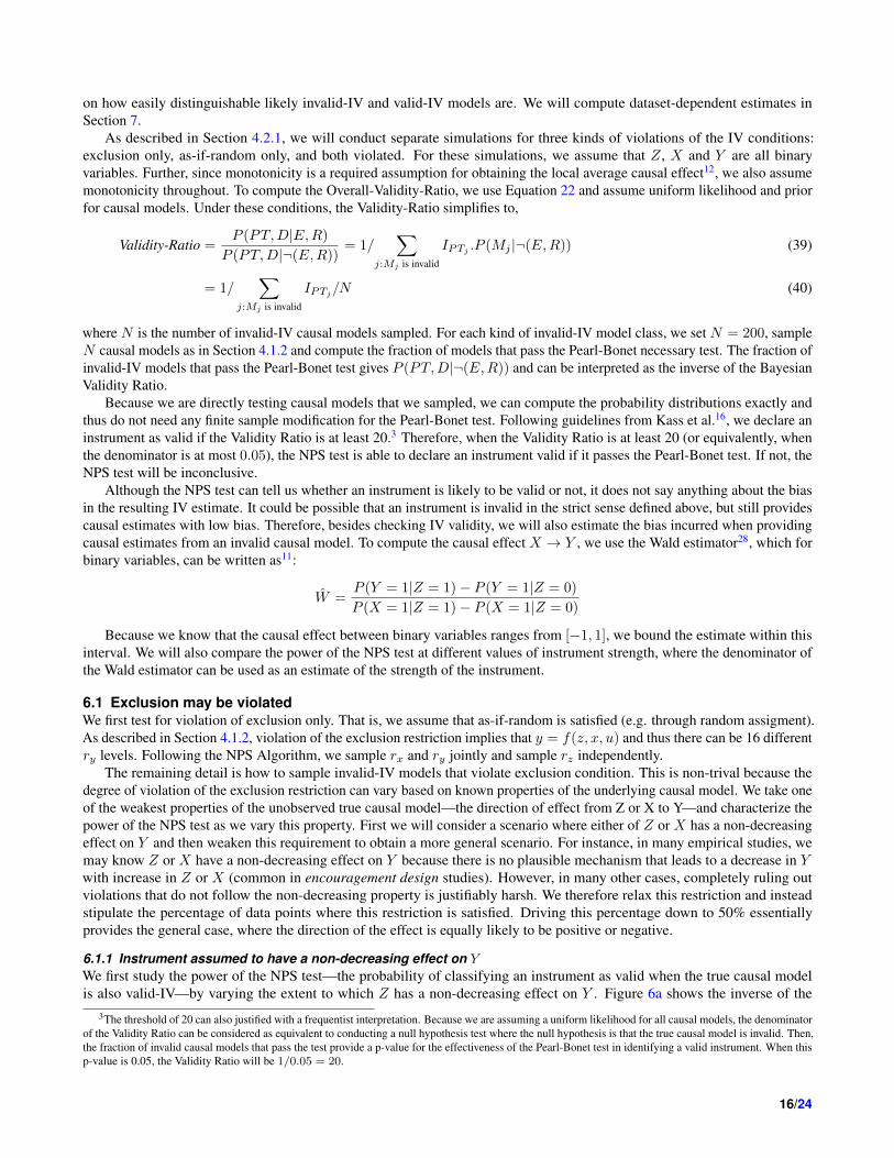
Log Marginal Likelihood

Dataset Exclusion Violated As-if-random Violated Valid IV Validity Ratio

D0 : Z,X, Y0 -3080 -3086 -3077 20.1D1 : Z,X, Y1 -3168 -3161 -3163 0.13D2 : Z,X, Y2 -3366 -3367 -3397 3.4x10−14

Table 1. Validity Ratio estimates for an example open problem proposed for testing binary instrumental variables. The NPStest can distinguish between valid-IV (D0) and invalid-IV (D1, D2) datasets. Bold values denote the maximum marginallikelihood for each dataset.

6.4 Summary of resultsTwo key patterns emerge. First, the test is more powerful in recognizing violations that also lead to a substantial bias. This isencouraging because the kind of violations that bias the causal estimate are exactly the invalid-IV datasets we want to eliminate.On average, these results suggest that when the NPS test is inconclusive, it is unlikely that applying the Wald Estimator willlead to substantial bias in the causal estimate. Conversely, in cases when the NPS test has high power, eliminating invalid-IVdata models will avoid computing Wald Estimates with high bias.

Second, the above results show that detecting the violation of IV conditions is sensitive to the strength of the instrument.This may seem as a big limitation; however, in most observational studies, instruments with high strength are rare. For instance,in economics,30 recommend an F-value of > 10 to prevent weak instrument bias. At such a low value for F , the instrument islikely to have to low correlation with X. Similarly, in epigenetics, R2 of 0.1 between Z and X is typical31. In these low strengthregimes, the NPS test can be effective in testing for validity of an instrumental variable, within some accepted false positive rate.

7 USING NPS TEST TO VALIDATE PAST IV STUDIESIn this section we evaluate the effectiveness of the NPS test in practice. First, we will apply the test to an open problem forbinary instrumental variables that was proposed as a limitation of Pearl-Bonet necessary test. Then, we will apply the test totwo seminal and highly cited studies on instrumental variables. Finally, we will use the NPS test to validate recent studies froma leading economics journal,American Economic Review.

7.1 An example open problem for binary instrumental variablesPalmer et al.32 proposed the following problem for binary variables where the Pearl-Bonet necessary test fails to detect violationof IV assumptions. Let Z, X , Y be three binary variables generated from the following causal process:

Z ∼Bern(0.5)

U ∼Bern(0.5)

X ∼Bern(pX); pX = 0.05 + 0.1Z + 0.1U

Y0 ∼Bern(p0); p0 = 0.1 + 0.05X + 0.1U

Y1 ∼Bern(p1); p1 = 0.1 + 0.2Z + 0.05X + 0.1U

Y2 ∼Bern(p2); p2 = 0.1 + 0.05Z + 0.05X + 0.1U (41)

There can be three possible datasets: D0(Z,X, Y0), D1(Z,X, Y1),D2(Z,X, Y2). Z is a valid instrument only when theoutcome is Y0, not for Y1 and Y2. Although Pearl-Bonet test is able to rule out D1 as an invalid-IV dataset, Palmer et al. findthat it is inconclusive for D0 and D2. We validate the same datasets using the NPS test by simulating 2000 data points for eachdataset. Table 1 shows that comparing Validity-Ratio from the NPS test can be used to idntify the datasets for which Z is a validinstrument. The second and third columns show the log marginal likelihood for invalid-IV models when either of exclusionor as-if-random is violated. In the absence of additional information, we can assume a uniform prior over valid-IV versusinvalid-IV models (P (M1 = P (M2). This leads to the Validity Ratio computed in the fifth column, as a ratio of marginallikelihood of the Valid-IV model class over marginal likelihood of the Invalid-IV model class. Validity Ratio is the highest(nearly 20) for D0 and the lowest (< 10−13) for D2, thereby clearly distinguishing between the two datasets. Dataset D1 has aValidity Ratio less than 1, indicating that it is less likely to be a valid instrument, especially in comparison to dataset D0.

In practice, a common goal is to select a single instrument. Results from the NPS test indicate that D0 should be chosen; ithas the highest Validity-Ratio among candidate datasets. Further, given that the Validity-Ratio is greater than 1, it is also likelyto be a valid instrument. As a guidance, we suggest following standard thresholds for the Bayes Factor in determining when the

20/24

●

●

●

●

●

●

●●

●

●

0.00

0.25

0.50

0.75

1.00

0 1 2 3 4 5 6 7 8 9Year of birth (0−9)

Like

lihoo

d as

sum

ing

inst

rum

ent i

s va

lid

Decade of birth ● 20 30 40 Necessary inequalities satisfied ● ●No Yes

(a) Unconditional IV

●●

●

●

●●

●

●

●

●

0.0

0.2

0.4

0.6

0.8

0 1 2 3 4 5 6 7 8 9Year of birth (0−9)

Like

lihoo

d as

sum

ing

inst

rum

ent i

s va

lid

Decade of birth ● 20 30 40 Necessary inequalities satisfied ● ●No Yes

(b) Conditional IV

Figure 9. Likelihood of being generated from a valid-IV causal model for instruments used in a past IV study, as provided bythe output of the necessary test. Left panel shows unconditional instruments, while the right panel instruments conditioned onrelevant covariates. Many of the instruments used have a likelihood below 0.05.

Validity-Ratio is high enough?. However, we deliberately refrain from providing standard thresholds, because the judgment forvalidity of an instrument will anyways depend on the prior assumed for Invalid-IV and Valid-IV model classes. We recommendinterpreting the ratio of marginal likelihoods as a benchmark for priors: a Validity Ratio of 20 assuming uniform priors indicatesthat for D0 to be an invalid-IV dataset, a researcher’s prior on finding an invalid-IV dataset should be at least 20 times as strongas the prior for valid-IV dataset.

7.2 Seminal IV studies on the effect of schooling on wagesReturns of schooling on future income was one of the first applications that instrumental variable studies were applied to. Weapply the NPS test to two of the seminal instrumental variable studies1, 33. These studies are both highly cited, yet concernsabout their validity continue until today29, 34. We show how the NPS test can provide evidence and validate the instrumentsused in these studies.

7.2.1 Effect of compulsory schooling on future wagesThe first paper estimates the effect of compulsory schooling on future earnings of students1. In the original analysis, Z isthe quarter of birth, which was binarized to indicate that the student was either born in the first quarter or the last threequarters. X is years of schooling and Y is the (log) weekly earnings of individuals. Using yearly cohorts, the authors define aseparate instrumental variable for each year of birth. The causal effect of interest is the effect of years of schooling on futureearnings.4 Years of schooling and earnings are both reported as continuous numbers, in a bounded range. We follow thesimplest discretization by binarizing both these variables at their mean. To check robustness against outliers, we also tried usingmedian as the cutoff and obtained similar results.

As in the original paper, we first use the IV method without conditioning on any covariates. of Applying the NPS test showsthat 3 out of yearly instruments do not pass the necessary test at a significance level of α = 0.05, as Figure 9a shows. Thisindicates that one or more of the three assumptions—monotonicity, exclusion and as-if-random—is violated, at least whenall variables are binary. Further, interpreting the p-value of the necessary test as the likelihood of the observed data beinggenerated from a valid-IV causal model, Figure 9a shows that nearly half of the instruments have less than 50% likelihood ofbeing generated from a valid-IV causal model. Although we cannot rule out that some of them may be valid, we can use thelikelihood values from the necessary test to filter out instruments that more likely to be valid and thus compute more reliableestimates.

In practice, however, unconditional instrumental variables are rare. The original paper proceeds to construct conditionalinstrumental variables based on related covariates in the dataset. We replicate conditioning on covariates by implementing apartialling out strategy?. Based on the Frisch-Waugh-Lovell theorem, using the partialling out technique provides the equivalenteffect of conditioning on covariates, provided the underlying causal model is linear (which the authors assume). Figure 9b

4Dataset available at http://economics.mit.edu/faculty/angrist/data1/data/angkru1991

21/24

http://economics.mit.edu/faculty/angrist/data1/data/angkru1991

Study name Num. Observations IV Strength Pearl-Bonet Test Result Validity Ratio

Randomized ExperimentNational Job Training Partnership Act (JTPA) Study (2002)35

5102 0.58 Pass 3.4Instrumental Variable StudiesEffect of rural electrification on employment in South Africa (2011)36

–Type 0 1816 0.1 Pass 3.6–Type 1 1816 0.1 Fail (p=0.26) 0.002–Type 2 1816 0.16 Fail (p=0.16) 0.0009–Type 3 1816 0.05 Fail (p=0.11) 0.001Effect of Chinese import competition on local labor markets (2013)37

–Outcome(population change) 1444 0.59 Pass 0.3–Outcome(employment) 1444 0.59 Pass 0.3Effect of credit supply on housing prices (2015)38

–Outcome(nloans) 11107 -0.009 Fail (p=0.003) 0.011–Outcome(vloans) 11107 -0.003 Fail (p=0.005) 0.006–Outcome(lir) 11107 -0.01 Fail (p=0.004) 0.0004Effect of subsidy manipulation on Medicare premiums (2015)39

–Unconditioned 170 0.60 Pass 1.02–Conditioned 170 0.42 Pass 0.04Effect of Mexican immigration on crime in United States (2015)40

–Unconditioned 182 0.50 Pass 0.07–Conditioned 182 0.22 Pass 0.005

Table 2. Split on mean.

shows the results of the necessary test when all instruments are conditioned on covariates. Contrary to intuition, a biggerfraction of conditional instruments are now invalid at the 5% significance level using the necessary test. Combined, our resultson unconditional and conditional IVs suggest that many of the instruments used in the original analysis may not be valid, atleast when the treatment and outcome is binarized.

7.2.2 Return of college education on future earningsAnother early study in the instrumental variables literature was on the effect of college education on future earnings of students33.This study used a person’s distance from college as an instrument to estimate the causal effect of college education. We follow asimilar protocol as above. Z is distance from college, which was already binarized in the original study. X is years of educationand Y is the log weekly wages.5 After binarizing X and Y , data from Card does not pass the necessary test for IV validity.

7.3 Recent IV studies in the American Economic ReviewWe now apply the NPS test to validate more recent IV studies. To select recent studies, we searched for papers published inthe American Economic Review from 2011-2015 that had ‘instrumental variable” or “instrument” mentioned in their title orabstract. From this set, we filtered out studies that did not provide full datasets for replication, leaving us with five studies onthe causal effect of diverse economic treatments such as rural electrification36, credit supply38, subsidy manipulation39, foreignimport competition37, and foreign immigration40. As a comparison benchmark, we also include an instrumental variable studybased on data from a randomized experiment35, which almost surely should pass the NPS test.

For each of the studies, we use code provided by the authors to construct a dataset of three variables (Z,X, Y ), where Zis the instrument. If the authors condition on covariates, then we use the partialling out technique to process the (Z,X, Y )dataset. Finally, we binarize each variable at its mean, unless it is already binarized. Table 2 presents results from the NPS test.First, we find that the randomized experiment passes the Pearl-Bonet test and obtains a Validity Ratio of 3.4, thus providing aweak evidence for a valid instrument. In contrast, 2 out of 5 do not pass Pearl-Bonet test when binarized. They also reportsignificantly low estimates of the Validity Ratio. For the other three studies, the Validity Ratio is less than 1, even thoughthey pass the Pearl-Bonet necessary test. This suggests that the data does not support validity of the instruments used. As anexample, the conditional instrument for the study on Mexican immigration obtains a Validity Ratio of 0.005, providing strong

5Dataset available at http://davidcard.berkeley.edu/data_sets.html

22/24

http://davidcard.berkeley.edu/data_sets.html

evidence for the invalidity of the instrument. However, in the other two studies the Validity Ratio is high enough that we cannotreject the validity of the instrument, thereby proving inconclusive about their validity.

8 DISCUSSION AND FUTURE WORKWe presented a probably sufficient test for instrumental variables using necessary tests proposed by past work. Simulationresults show that the effectiveness of the test increases as the strength of the instrument decreases. Therefore, while the NPS testcannot always verify whether an instrument is valid, it can do so when the instrument is weak. Fortunately, many observationalstudies are based on instruments with low Z-X correlation, where NPS can be applied. Future work includes studying thesensitivity of the NPS test to different discretization strategies and different priors on causal models.

More generally, the NPS test is an example of a general Bayesian testing framework for causal models. When necessaryexistence tests based on specific causal models are available, they can be used to create a probably sufficient test. We haveshown that the combined evidence from the observed data and a necessary test can be used to distinguish between causalmodels. Looking forward, the proposed test can be used to compare potential instruments for their validity, allow transparentcomparisons between multiple IV studies, and enable a data-driven search for natural experiments.

AcknowledgementsWe acknowledge Jake Hofman and Duncan Watts for their valuable feedback throughout the course of this work. We also thankMiro Dudik, Akshay Krishnamurthy, Justin Rao, Vasilis Syrgkanis and Michael Zhao for helpful suggestions.

References1. Angrist, J. D. & Krueger, A. B. Does compulsory school attendance affect schooling and earnings? Quarterly Journal of

Economics 106, 979–1014 (1991).

2. Angrist, J. D. & Pischke, J.-S. Mostly harmless econometrics: An empiricist’s companion (Princeton university press,2008).

3. Lawlor, D. A., Harbord, R. M., Sterne, J. A., Timpson, N. & Davey Smith, G. Mendelian randomization: using genes asinstruments for making causal inferences in epidemiology. Statistics in medicine 27, 1133–1163 (2008).

4. Stuart, E. A. Matching methods for causal inference: A review and a look forward. Statistical science: a review journal ofthe Institute of Mathematical Statistics 25, 1 (2010).

5. Pearl, J. On the testability of causal models with latent and instrumental variables. In Proceedings of the Eleventhconference on Uncertainty in artificial intelligence, 435–443 (Morgan Kaufmann Publishers Inc., 1995).

6. Bonet, B. Instrumentality tests revisited. In Proceedings of the Seventeenth conference on Uncertainty in artificialintelligence, 48–55 (Morgan Kaufmann Publishers Inc., 2001).

7. Nakamura, A. & Nakamura, M. On the relationships among several specification error tests presented by durbin, wu, andhausman. Econometrica: journal of the Econometric Society 1583–1588 (1981).

8. Morgan, S. L. & Winship, C. Counterfactuals and causal inference (Cambridge University Press, 2014).

9. Dunning, T. Natural experiments in the social sciences: a design-based approach (Cambridge University Press, 2012).

10. Sharma, A., Hofman, J. M. & Watts, D. J. Split-door criterion for causal identification: Automatic search for naturalexperiments. arXiv preprint arXiv:1611.09414 (2016).

11. Balke, A. & Pearl, J. Nonparametric bounds on causal effects from partial compliance data. Technical report, UCLA(1993).

12. Angrist, J. & Imbens, G. Identification and estimation of local average treatment effects. Econometrica (1994).

13. Ramsahai, R. & Lauritzen, S. Likelihood analysis of the binary instrumental variable model. Biometrika 98, 987–994(2011).

14. Kitagawa, T. A test for instrument validity. Econometrica 83, 2043–2063 (2015).

15. Koller, D. & Friedman, N. Probabilistic graphical models: principles and techniques (MIT press, 2009).

16. Kass, R. E. & Raftery, A. E. Bayes factors. Journal of the american statistical association 90, 773–795 (1995).

17. Balke, A. & Pearl, J. Probabilistic evaluation of counterfactual queries. Proc. of AAAI (1994).

18. Heckerman, D. & Shachter, R. Decision-theoretic foundations for causal reasoning. Journal of Artificial IntelligenceResearch 405–430 (1995).

23/24

19. Hankin, R. K. et al. A generalization of the dirichlet distribution. Journal of Statistical Software 33, 1–18 (2010).

20. Cooper, G. F. & Herskovits, E. A bayesian method for the induction of probabilistic networks from data. Machine learning9, 309–347 (1992).

21. Genz, A. & Cools, R. An adaptive numerical cubature algorithm for simplices. ACM Transactions on MathematicalSoftware (TOMS) 29, 297–308 (2003).

22. Neal, R. M. Annealed importance sampling. Statistics and Computing 11, 125–139 (2001).

23. Skilling, J. et al. Nested sampling for general bayesian computation. Bayesian analysis 1, 833–859 (2006).

24. Feroz, F., Hobson, M. & Bridges, M. Multinest: an efficient and robust bayesian inference tool for cosmology and particlephysics. Monthly Notices of the Royal Astronomical Society 398, 1601–1614 (2009).

25. Chaves, R. et al. Inferring latent structures via information inequalities. arXiv preprint arXiv:1407.2256 (2014).

26. Huber, M. & Mellace, G. Testing instrument validity for late identification based on inequality moment constraints. Reviewof Economics and Statistics 97, 398–411 (2015).

27. Wang, L., Robins, J. M. & Richardson, T. S. On falsification of the binary instrumental variable model. arXiv preprintarXiv:1605.03677 (2016).

28. Wald, A. The fitting of straight lines if both variables are subject to error. The Annals of Mathematical Statistics 11,284–300 (1940).

29. Bound, J., Jaeger, D. A. & Baker, R. M. Problems with instrumental variables estimation when the correlation between theinstruments and the endogenous explanatory variable is weak. Journal of the American statistical association 90, 443–450(1995).

30. Staiger, D. O. & Stock, J. H. Instrumental variables regression with weak instruments (1994).

31. Pierce, B. L., Ahsan, H. & VanderWeele, T. J. Power and instrument strength requirements for mendelian randomizationstudies using multiple genetic variants. International journal of epidemiology dyq151 (2010).

32. Palmer, T. M., Ramsahai, R. R., Didelez, V., Sheehan, N. A. et al. Nonparametric bounds for the causal effect in a binaryinstrumental-variable model. Stata Journal 11, 345 (2011).

33. Card, D. Using geographic variation in college proximity to estimate the return to schooling. Tech. Rep., National Bureauof Economic Research (1993).

34. Buckles, K. S. & Hungerman, D. M. Season of birth and later outcomes: Old questions, new answers. Review of Economicsand Statistics 95, 711–724 (2013).

35. Abadie, A., Angrist, J. & Imbens, G. Instrumental variables estimates of the effect of subsidized training on the quantilesof trainee earnings. Econometrica 70, 91–117 (2002).

36. Dinkelman, T. The effects of rural electrification on employment: New evidence from south africa. The American EconomicReview 101, 3078–3108 (2011).

37. David, H., Dorn, D. & Hanson, G. H. The china syndrome: Local labor market effects of import competition in the unitedstates. The American Economic Review 103, 2121–2168 (2013).

38. Favara, G. & Imbs, J. Credit supply and the price of housing. The American Economic Review 105, 958–992 (2015).

39. Decarolis, F. Medicare part d: are insurers gaming the low income subsidy design? The American Economic Review 105,1547–1580 (2015).

40. Chalfin, A. The long-run effect of mexican immigration on crime in us cities: Evidence from variation in mexican fertilityrates. The American Economic Review 105, 220–225 (2015).

24/24

necessary and probably sufﬁcient test for finding...

Documents