Near Term Algorithms for Linear Systems of Equations

Aidan Pellow-Jarman,1, ∗ Ilya Sinayskiy,2, 3, † Anban Pillay,1, 4, ‡ and Francesco Petruccione2, 3, §

1School of Mathematics, Statistics and Computer Science,University of KwaZulu-Natal, Durban, KwaZulu-Natal, 4001, South Africa

2Quantum Research Group, School of Chemistry and Physics,University of KwaZulu-Natal, Durban, KwaZulu-Natal, 4001, South Africa

3National Institute for Theoretical and Computational Sciences (NITheCS), South Africa4Centre for Artificial Intelligence Research (CAIR), cair.org.za

Finding solutions to systems of linear equations is a common problem in many areas of science andengineering, with much potential for a speed up on quantum devices. While the Harrow-Hassidim-Lloyd (HHL) quantum algorithm yields up to an exponential speed up over classical algorithmsin some cases, it requires a fault tolerant quantum computer, which is unlikely to be availablein the near-term. Thus, attention has turned to the investigation of quantum algorithms for noisyintermediate-scale quantum (NISQ) devices where several near-term approaches to solving systems oflinear equations have been proposed. This paper focuses on the Variational Quantum Linear Solvers(VQLS), and other closely related methods. This paper makes several contributions that include:the first application of the Evolutionary Ansatz to the VQLS (EAVQLS), the first implementation ofthe Logical Ansatz VQLS (LAVQLS), based on the Classical Combination of Quantum States (CQS)method , the first proof of principle demonstration of the CQS method on real quantum hardwareand a method for the implementation of the Adiabatic Ansatz (AAVQLS). These approaches areimplemented and contrasted.

I. INTRODUCTION

Systems of linear equations play an important role inmany areas of science and engineering, making the poten-tial quantum speed-up for solving them of great interest.Solving a system of N linear equations with N unknowns,

expressible as A~x = ~b, involves finding the unknown so-

lution vector ~x satisfying A~x = ~b. This is known as theLinear Systems Problem (LSP).

The Harrow-Hassidim-Lloyd (HHL) algorithm [1] is aproposed quantum algorithm for the quantum linear sys-tems problem (QLSP) [2], a quantum analogue of theLSP. The QLSP is stated as follows: Let A be an N ×Nhermitian matrix (however this algorithm is not limited

to a hermitian matrix) and let ~x and ~b be N dimensional

vectors, satisfying A~x = ~b, having corresponding quan-tum states |x〉 and |b〉, such that

|x〉 :=

∑i xi |i〉

||∑i xi |i〉||2

, (1)

|b〉 :=

∑i bi |i〉

||∑i bi |i〉||2

. (2)

If A is not hermitian, define A =(

0 AA† 0

), which is her-

mitian, and instead solve the equation A~y =(~b0

)and

solve for ~y =(

0~x

). Given access to matrix A by means

∗ aidanpellow@gmail.com† sinayskiy@ukzn.ac.za‡ pillayw4@ukzn.ac.za§ petruccione@ukzn.ac.za

of an oracle, and a unitary gate U such that U |0〉 = |b〉,output a quantum state |x′〉 such that |||x〉 − |x′〉||2 ≤ ε,where ε is the error-bound of the approximate solution.

The HHL algorithm is a quantum algorithms expectedto give a substantial speed-up over classical approaches,providing up to an exponential speed-up over known clas-sical algorithms in cases where the linear system is sparse,the condition number is low, and the actual solution vec-tor is not required to be read out, but instead some scalarmeasure on the solution vector is of interest. As withmany promising quantum algorithms, the HHL algorithmrequires a fault-tolerant quantum computer to be success-fully implemented, predicted to only be available in thelong term future.

Approaches at finding algorithms for noisyintermediate-scale quantum (NISQ) devices [3], availablein the near-term future, have focused mainly on a classof algorithms known as Variational Hybrid QuantumClassical Algorithms (VHQCAs). The idea behindVHQCAs is to utilize a quantum-classical feedbackloop. Here a quantum device is used to compute a costfunction for a parameterized quantum circuit (ansatz),much more efficiently than is possible on a classicaldevice[6], while a classical device is used to optimise theselection of the ansatz parameters. VHQCAs rely on theuse of short depth quantum circuits to make them moreresistant to noise and allowing them to be successfullyrun on NISQ quantum hardware. The main difficultiesof this approach lie in overcoming the noise inherentin quantum devices and the difficulty of optimizing theansatz parameters. An example of these difficulties isthe barren plateau problem [4].

The Variational Quantum Eigensolver (VQE) [5] is onenotable VHQCA that solves the optimization problem,

arX

iv:2

108.

1136

2v1

[qu

ant-

ph]

25

Aug

202

1

2

E = minθ〈V (θ)|H |V (θ)〉 , (3)

whereby the minimum eigenvalue E of some HamiltonianH is approximated through the optimization of θ for someansatz V (θ).

The Variational Quantum Linear Solver [6, 7] is basedon the VQE, recently proposed to solve the quantum lin-ear systems problem. Since its proposal, many varia-tions have also been presented in order to overcome var-ious difficulties faced by the algorithm, and VHQCAs ingeneral. Attempts to combat these difficulties includetraining approaches like the Adiabatic Assisted VQE [7]and ansatz variations such as the Logical Ansatz, being aClassical Combination of various Ansatze [7, 8] and theEvolutionary Ansatz [9], an evolutionary approach forAnsatz construction. The evolutionary ansatz was ini-tially proposed for use in the VQE and has been appliedhere for the VQLS variation. Another non-variationalapproach to solving the quantum linear systems problemis the Classical Combination of Quantum States (CQS)method [7], of which the Logical Ansatz approach out-lined in this paper is an adaption.

The following approaches were implemented and willbe discussed in this paper:

Variational Quantum Linear Solver (VQLS)Adiabatic Ansatz VQLS (AAVQLS)Evolutionary Ansatz VQLS (EAVQLS)Classical Combination of Quantum State (CQS)Logical Ansatz VQLS (LAVQLS)

This paper makes several contributions to the litera-ture on the VQLS. Firstly, we present the first applicationof the Evolutionary Ansatz to the VQLS. The Evolution-ary Ansatz has previously been applied to the VariationalQuantum Eigensolver [9]. Secondly, the implementationproposed for solving systems of linear equations using theAAVQLS is also new to this work. Also, the first proofof principle demonstration of the CQS method on a realquantum device is conducted. Lastly, the first known im-plementation of the Logical Ansatz VQLS is given, withproposed training methods that are new to this work.All implementations of these approaches may be foundin the Github repository [? ].

This paper begins with a description of the above near-term approaches for the Quantum Linear Systems Prob-lem. Some experiments designed for an evaluation ofthese approaches are outlined in the section followingthat. We then present and discuss the results of the ex-periments.

II. NEAR-TERM ALGORITHMS

The inputs to the all the near-term algorithms below

are the matrix A, and vector ~b. A is given in a slightlydifferent form here than in the QLSP. Here A is given

by m unitary matrices Ai, implemented as unitary gates,such that A =

∑mi=1 ciAi, ci ∈ C (any hermitian matrix

in a finite-dimensional space can be written as a linearcombination of unitary matrices). Also given is a unitarygate U, such that U |0〉 = |b〉. VQLS cost functions oftenrequire either or both Ai and U to be given as controlledgates, which is assumed possible.

A. Variational Quantum Linear Solver

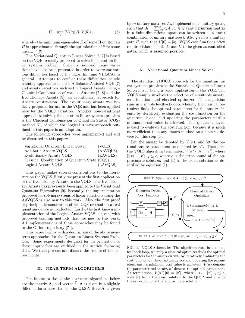
The standard VHQCA approach for the quantum lin-ear systems problem is the Variational Quantum LinearSolver, itself being a basic application of the VQE. TheVQLS simply involves the selection of a suitable ansatz,cost function, and classical optimizer. The algorithmruns in a simple feedback-loop, whereby the classical op-timizer finds the optimal parameters for the ansatz cir-cuit, by iteratively evaluating the cost function on thequantum device, and updating the parameters until aminimum cost value is achieved. The quantum deviceis used to evaluate the cost function, because it is muchmore efficient than any known method on a classical de-vice for this step [6].

Let the ansatz be denoted by V (α), and let the op-timal ansatz parameters be denoted by α∗. Then oncethe VQLS algorithm terminates, V (α∗) |0〉 = |x′〉, where|||x〉 − |x′〉||2 ≤ ε, where ε is the error-bound of the ap-proximate solution, and |x〉 is the exact solution as de-scribed by equation (I).

FIG. 1. VQLS Schematic: The algorithm runs in a simplefeedback loop, whereby a classical optimizer finds the optimalparameters for the ansatz circuit, by iteratively evaluating thecost function on the quantum device and updating the param-eters, until a minimum cost value is achieved. V (α) denotesthe parameterized ansatz, α∗ denotes the optimal parameters.At termination, V (α∗) |0〉 = |x′〉, where |||x〉 − |x′〉||2 ≤ ε,with |x〉 being the exact solution to the QLSP, and ε beingthe error-bound of the approximate solution.

3

1. VQLS Ansatz

Broadly speaking there are two types of ansatze;hardware-efficient (agnostic) ansatze and problem-specific ansatze.

Hardware-efficient ansatze are designed without tak-ing into account the specific problem being solved, thatis matrix A and |b〉, but rather only the topology (back-end connectivity of the qubits) and available gates of aspecific quantum computer. A hardware-efficient ansatzcan be denoted by a sequence of n parameterized quan-tum gates as,

VAgnostic(α) = γ1(α1)γ2(α2) · · · γn(αn), (4)

where γi denotes a specific parameterized gate in thequantum circuit, and αi denotes that parameters value.

These ansatze can be constructed to be more resistantto noise on any specific available quantum device, butthey may fall short finding a solution |x′〉, as any partic-ular hardware-efficient ansatze is not guaranteed to spanthe region of the Hilbert space containing any good ap-proximation of the solution |x′〉. Therefore a hardware-efficient ansatz effectively trades potential relevance tothe specific problem, for increased noise resistance.

Problem-specific ansatze on the other hand do nottake into account the specific quantum device being used,and rather try to exploit the knowledge of the problemavailable. The Quantum Alternating Operator Ansatz(QAOA) [6] is one such proposed problem-specific ansatz,using two hamiltonians, known as the driver and themixer, denoted by HD and HM respectively, constructedfrom specific knowledge of the problem, namely A and~b. This problem-specific ansatz can be denoted by a re-peating sequence of driver and mixer hamiltonian simu-lations, each being applied for a variable amount of time.These time parameters α are the trainable aspect of thisproblem specific ansatz, which are optimized by someclassical device. The QAOA can be denoted as,

VQAOA(α) = e−iHMα2pe−iHDα2p−1 . . . e−iHMα2e−iHDα1 .(5)

The requirement of Hamiltonian simulation from theQAOA makes these ansatze far less near-term, there-fore these ansatze are not considered further in this pa-per. More information on the specific construction of theQAOA, including operators HD and HM is given in [6].

2. VQLS Cost Functions

The cost function Hamiltonian is where the applicationof the VQE algorithm to solving systems of linear equa-tions is implemented. Various different cost functions

have been proposed for the VQLS [6, 7]. For simplicity,denote the state V (α) |0〉, as |x〉, and let |ψ〉 = A |x〉. Ref.[6] proposes a cost function based on the overlap betweenthe projector |ψ〉〈ψ| and the subspace orthogonal to |b〉.This cost function also normalizes the expectation valueof the Hamiltonian to improve performance. The costfunction is given by,

CG =〈x|HG|x〉〈ψ|ψ〉

, (6)

where the Hamiltonian HG is given by,

HG = A†(1− |b〉〈b|))A. (7)

This cost function can have gradients that vanish expo-nentially with the number of qubits. To improve on thisshortfall, the cost function CL is proposed by replacingHG with a local version of the Hamiltonian, HL, improv-ing the trainability of the ansatz, given by,

HL = A†U(1− 1

n

n∑j=1

|0j〉〈0j | ⊗ 1j)U†A, (8)

where 1j denotes identity on all qubits except qubitj. The cost function CL can be computed using theHadamard Test as shown in Fig. 2. CL has been shownto be equivalent cost function to CG, however having im-proved performance [6], and is explicitly given by,

CL =〈x|HL|x〉〈ψ|ψ〉

. (9)

3. Classical Optimizers

The VQLS admits the use of either gradient-free orgradient-based optimizers. For gradient-based optimiz-ers, gradient values can be found analytically [6, 10],or estimated through finite differences. The classicaloptimizer chosen has a large impact on how well the op-timization process deals with the noise inherent in NISQdevices. Some classical optimizers handle noise betterthan others [11], making classical optimizer selection im-portant.

B. Adiabatic Assisted VQLS

The Adiabatic Assisted Variational Quantum LinearSolver (AAVQLS) [7], simply augments the standard

4

FIG. 2. Hadamard Test Circuits for cost function CL Eq. (9).The top circuit is employed when calculating the value of thenumerator 〈x|HL|x〉, while the bottom circuit is employedwhen calculating the value of the denominator, 〈ψ|ψ〉. TheS† gate, is included when calculating imaginary-valued partsof the cost function, and excluded when calculating the real-valued parts.

VQLS approach, by proposing a variation in the Hamil-tonian over time, inspired by adiabatic quantum com-puting methods [12], in an attempt to allow the ansatzstate to always be close to the ground state of the Hamil-tonian. Let H0 be a Hamiltonian with a known groundstate, and let H1 be the Hamiltonian whose ground statecorresponds to the solution of the linear system in ques-tion. Let the Hamiltonian of the AAVQLS be given by(1−s)H0 +sH1, where s is a discrete parameter, varyingfrom s = 0, to s = 1, in T discrete intervals, during theoptimization process.

This approach is the same as the VQLS with respectto the cost function and classical optimizer, however theansatz must be chosen such that it can be easily initial-ized in the ground state of H0 at the start of the algo-rithm. The only added procedure to the AAVQLS fromthe VQLS occurs during the training phase, where theparameter s is varied in T discrete intervals from s = 0to s = 1, thereby varying the hamiltonian from H0 toH1.

Proposed here is one way in which the AAVQLS canbe implemented as an adaption of the VQLS. Firstly thelinear system is reformulated as,

[(1− s)1 + sA]~x = ~b, (10)

where s can be varied from 0 to 1, with ~x = ~b, when

s = 0, and [(1 − s)1 + sA]~x = ~b, equivalent to A~x = ~b,when s = 1.

Then for a suitable ansatz V (α) =γ1(α1)γ2(α2) · · · γn(αn) where α can be initializedsuch that V (α) = 1, append to it the unitary U (for

creating state |b〉) to create ansatz VAAVQLS(α) asbelow,

VAAVQLS(α) = UV (α). (11)

Here VAAVQLS |0〉 is indeed be equal to |b〉 when α isinitialized appropriately (such that V (α) = 1).

The AAVQLS algorithm then proceeds as follows:

1. Let s = 0 and let ansatz parameters α = α∗, suchthat V (α∗) is equal to 1. Then VAAVQLS(α) givesthe solution to (9). Let αprevious = α.

2. Increment s by 1T .

3. Using the VQLS approach, with initial ansatz pa-rameters set to αprevious, find the new optimal pa-rameters αcurrent with ansatz VAAVQLS.

4. Let αprevious = αcurrent and if s 6= 1 return to step2; else αfinal = αcurrent.

5. VAAVQLS(αfinal) |0〉 = |x′〉, where |||x〉 − |x′〉|| ≤ ε,where |x〉 is the exact solution to the QLSP and εis the error-bound of the approximate solution.

C. Evolutionary Ansatz VQLS

The Evolutionary Ansatz [9] utilises a genetic algo-rithm to construct the parameterized quantum circuit,while concurrently optimising its parameters. This ap-proach adapts the ansatz structure to both the specifiedproblem and the backend configuration of the quantumdevice available, so it can be thought of as constructingan ansatz that is both hardware-efficient and problem-specific. This specialized ansatz would be highly noiseresistant (being shallower and requiring fewer 2-qubitgates) while remaining applicable to the specific prob-lem being solved. This approach still requires a VQLScost function and classical minimizer, as standard in withVQLS.

The main outline of the Evolutionary Ansatz algorithmis presented here. For a full explanation please see theoriginal paper[9]. Some specific details about the evo-lutionary ansatz implementation in this discussion differfrom the original paper.

Evolutionary Algorithms are based on the principleof natural selection. The Evolutionary Ansatz VQLS(EAVQLS) mimics this principle to adapt the ansatzchoice by evolving a set of candidate ansatze, knownas the population, through random mutations (theEAVQLS only mimics asexual reproduction, there areno crossovers between candidate solutions in the popu-lation). The candidate ansatze being evolved are knownas genomes. A genome consists of a list of genes, and forthe EAVQLS is given as follows. If Vi(α) is any potentialansatz in the population, Vi(α) is expressed as a genomegi that can be written as,

5

gi = [γ1(α1), γ2(α2), · · · , γm(αm)],

where each γi is a gene. Each gene γi is a layer of gatessuch that each qubit of the ansatz is assigned a gate.This set of gates is chosen from a gate set,

G = {I2, U3,∧1U3},

where I2 is the single qubit identity gate, U3 is the uni-versal single qubit rotation, and ∧1U3 is the controlledversion of U3. Other gate sets may be used, for example,if the VQLS problem only deals with real valued A and~b, an appropriate gate set is given by,

GR = {I2, Ry,∧1Ry}.

An example of an evolutionary ansatz genome is shownin Fig. 3.

FIG. 3. 4 Qubit Evolutionary Ansatz Genome Schematic:Three different genes (ansatz rows) are each outlined in red,blue and green in the genome above. The qubits are initializedas H⊗n |0〉⊗n, allowing the first gene in the genome to containcontrolled gates that aren’t redundant.

Initially, the evolutionary algorithm begins with a pop-ulation consisting of random genomes, each only consist-ing of a single gene. The qubits in all ansatz circuitsare initialized with the gate H⊗n, allowing the first genein the genome to contain controlled gates that aren’t re-dundant when the ansatz corresponding to the genomeis applied to the state |0〉⊗n. These genomes are evolvedasexually, through the use of 3 genetic operators, topo-logical search, parameter search and removal.

The topological search operator, τ , explores the spaceof possible ansatze, by adding a new random gene tothe genome, which is equivalent to adding a new randomlayer of gates to the ansatz represented by the genome.The new gene added to the genome is initialized as iden-tity, to ensure that the genome’s fitness may only im-prove, or at worst, remain the same. The new gene

added to the genome also takes into account the gatesof the previous gene in the genome, eliminating poten-tial redundant gates (two of the same gate on the samequbit/s in a row) being added to the genome with thenew gene. The identity gate, I2, is only used wheneveradding a different gate would cause some redundancy.The operation performed by τ is given by,

τ : [γ1(α1), · · · , γm(αm)] −→[γ1(α1), · · · , γm(αm), γm+1(αm+1)].

The removal operator, ρ, acting on a genome, removessome number of genes from the genome, starting fromthe end of the gene list. The operation performed by ρis given by,

ρ : [γ1(α1), · · · , γp(αp), · · · , γm(αm)] −→[γ1(α1), γ2(α2), · · · , γp(αp)]

where p ∈ {1, 2, · · · ,m}.The parameter search runs an optimization subroutine,

O, on each individual gene in the genome, in a randomorder. The optimization subroutine O is implementedfor a genome gi and a gene yi(αi), by using the ansatzV (α) represented by genome gi in the standard VQLSoptimization routine, while only optimizing the specificparameters αi of the gene yi(αi). This optimization isdone per gene so that removal operator does not affectthe training of the rest of the ansatz.

The fitness fi, of genome gi is calculated using thevalue of the cost achieved by the ansatz represented bythe genome, as well as the depth of the ansatz (numberof genes) and the number of 2-qubit gates. The fitnessvalue is given by,

fi = C(gi) + α · |gi|+ β · |∧(gi)|,

where α and β are weighted variables that can be as-signed, C(gi) is the cost value of the ansatz of repre-sented by gi, |gi| is the number of genes in gi, and |∧(gi)|is the number of 2-qubit gates in gi. This genome fit-ness value is then averaged amongst genomes of the samespecies and is called the species-adjusted fitness. Speciesare defined by a genetic distance measure, given by theaverage distance of a common ancestor between two sep-arate genomes. Two genomes with an average distanceof a common ancestor less than some given value may beassigned to the same species.

The EAVQLS Algorithm runs as follows:

1. Generate a population P of n empty genomes gi,and apply τ(gi) to each genome.

2. Apply the optimization subroutine O to the lastgene in each genome for all genomes in P .

3. Group the genomes in P by species, then calculatethe fitness and then species-adjusted fitness of eachgenome gi in P .

4. Randomly select n parent genomes with replace-ment from P , inversely proportional to their fitnessvalues, forming the next generation P ′.

6

5. For all of the genomes gi in P ′, apply the threegenetic operators to gi with some predefined prob-abilities.

6. If a termination condition is met, return the fittestgenome in P ′, else let P = P ′ and return to step 2.

D. Classical Combination of Quantum States(CQS)

The Classical Combination of Quantum States (CQS)approach detailed in [7], is the most unique near-termapproach presented in this paper. The CQS approach isnot a variational algorithm, meaning there is no classicaloptimisation of ansatz parameters. The CQS approachsolves the linear system by finding the solution as a linearcombination of quantum states.

Given a set of n states S = {|s1〉 , · · · , |sn〉}, the CQSmethod aims to find a linear combination x′ approximat-

ing the solution x to the linear systems problem A~x = ~bwhere,

x′ =

n∑i=1

αi |si〉 , α ∈ C. (12)

Note that, differing from the above mentioned ap-proaches, the solution x′ is never actually created on thequantum device. It is not necessarily normalized, and isproportional to the solution to the same problem solvedusing the other variational methods.

The CQS Algorithm runs as follows. Starting withm = 1, and the set S = {|s1〉} where |s1〉 is a state thatcan be prepared by some efficient quantum circuit.

1. Solve the for the optimal values of α∗ such thatx′ = Σmi=1α

∗i |si〉, where x′ is the an approximation

of x, given the set S.

2. Using the value of α∗, find the next circuit gener-ating the state |sm+1〉 and add |sm+1〉 to S.

3. Set m = m+ 1 and repeat from step 1 until x′ is asufficiently good solution.

Given a set of n efficiently prepared states, S ={|s1〉 , · · · , |sn〉}, containing a close approximation of thesolution x as a linear combination, the linear coefficients,ci, can be found efficiently by a hybrid quantum-classicalprocedure outlined below.

The standard regression function used to solve a linearsystem is given by,

LR(x) := ||Ax− |b〉||22 = x†A†Ax− 2Re[〈b|Ax] + 1.(13)

Given x =∑mi=1 αi |si〉, let V = (v1, . . . , vm) where vi =

A |si〉. Now Ax =∑mi=1 αiA |si〉 = V α. Eq. (13) can be

rewritten as,

||V α− |b〉||22 = α†V †V α− 2Re{q†α}+ 1. (14)

where qi = 〈i|V † |b〉 = 〈si|A† |b〉. A simple regressionproblem for α can be obtained with the kernel matrixV †V , where (V †V )ij = 〈si|A†A |sj〉. This quadratic op-timization problem on complex α can be rewritten as areal optimization problem,

minz(z†Qz − 2rT z + 1), (15)

where z = (Re[α], Im[α]), and Q and r are given by,

Q =

(Re[V †V ] Im[V †V ]Im[V †V ] Re[V †V ]

), (16)

r =(Re[q] Im[q]

). (17)

Here Eq. (15) can be solved using standard convexquadratic programming methods.

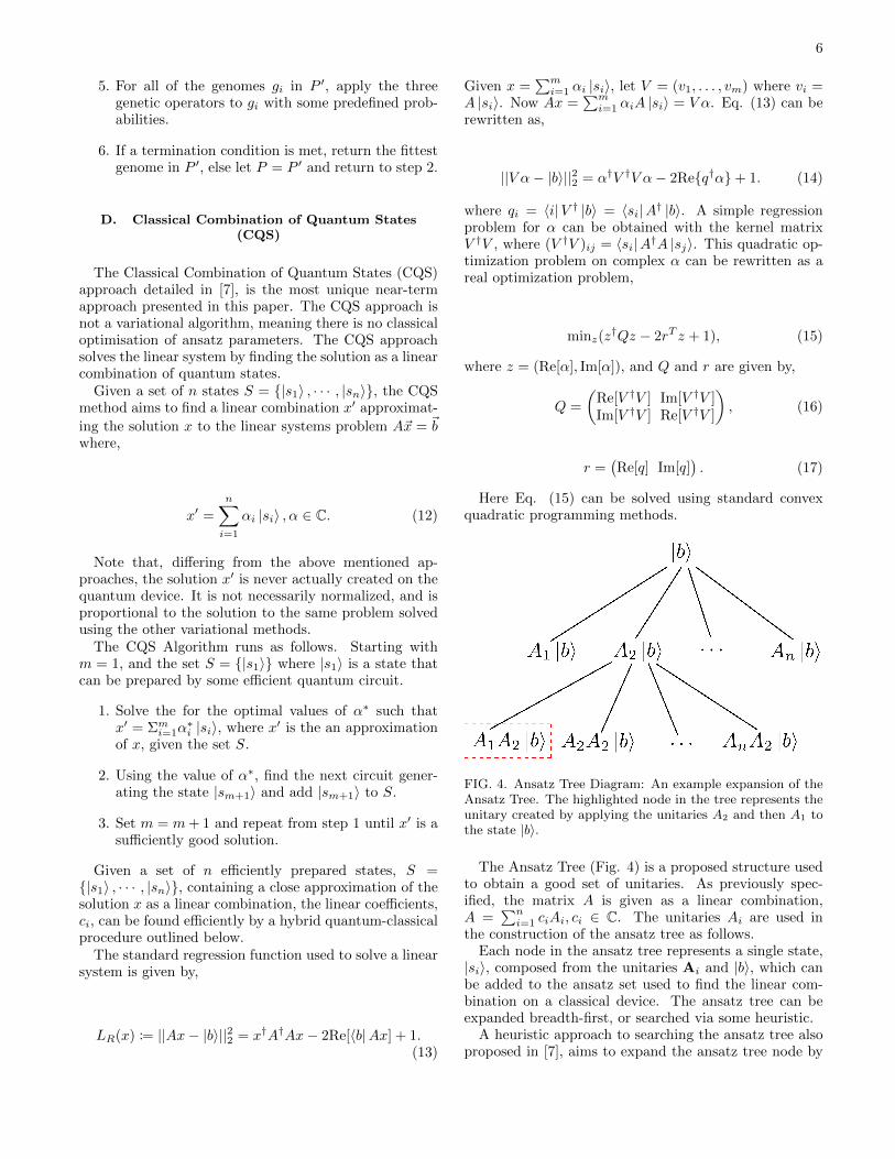
FIG. 4. Ansatz Tree Diagram: An example expansion of theAnsatz Tree. The highlighted node in the tree represents theunitary created by applying the unitaries A2 and then A1 tothe state |b〉.

The Ansatz Tree (Fig. 4) is a proposed structure usedto obtain a good set of unitaries. As previously spec-ified, the matrix A is given as a linear combination,A =

∑ni=1 ciAi, ci ∈ C. The unitaries Ai are used in

the construction of the ansatz tree as follows.Each node in the ansatz tree represents a single state,|si〉, composed from the unitaries Ai and |b〉, which canbe added to the ansatz set used to find the linear com-bination on a classical device. The ansatz tree can beexpanded breadth-first, or searched via some heuristic.

A heuristic approach to searching the ansatz tree alsoproposed in [7], aims to expand the ansatz tree node by

7

node. Let the current set of expanded nodes in the treebe given by the set S, and the current set of all poten-tial child nodes of the nodes in S be the set C (S). Letthe current approximate solution for the set of expandednodes be given by α∗. The ansatz tree is further exploredby expanding the child node, |ψ〉 ∈ C (S), that has thegreatest overlap with the current gradient, maximizingthe function given by,

〈ψ| ∇LR(xs) = 2∑|ψi〉∈S

α∗i 〈ψ|A2 |ψi〉 − 2 〈ψ|A |b〉 . (18)

E. Logical Ansatz VQLS

The logical ansatz approach is simply an adaptionof the CQS method above, allowing for parameterizedunitaries to be employed. This approach is then simi-lar to the Standard VQLS approach, except it proposesthat instead of a single ansatz circuit, a linear combi-nation of multiple ansatz circuits be used. This greatlylowers the depth of any one of the multiple ansatz cir-cuits. The Logical Ansatz is implemented here as sug-gested in [7], by implementing the CQS method witha selected set of n parameterized ansatze making thestates S = {|s1(θ1)〉 , · · · , |sn(θn)〉}, and repeating theoptimization process outlined for the CQS with a classi-cal minimizer optimizing the parameters θi of the ansatzecreating the states |si(θi)〉. This method avoids theansatz tree expansion process for selecting unitaries, byinstead optimizing a set of pre-selected parameterizedunitaries. The solution found is expressed by,

x′ =

n∑i=1

αi |si(θi)〉 , αi ∈ C. (19)

This logical ansatz implementation and training differsfrom that in [8].

The Logical Ansatz Linear Solver Algorithm runsmuch like the CQS method.

1. Select n parameterized ansatze each correspondingto some state |si(θi)〉, forming set S.

2. Solve the for the optimal value of α∗ such thatx′ = Σmi=1α

∗i |si(θi)〉, where x′ is the closest ap-

proximation of x, given the set S. Proceed eitherto 3 or 4 for method 1 or 2 respectively.

3. Method 1: For r training rounds, select each of thestates |si(θi)〉 at random and optimize their param-eters θi with some classical optimizer, only solvingthe new α∗ value after the parameter optimizationof each ansatz.

4. Method 2: Treating the entire state x′ =Σmi=1α

∗i |si(θi)〉 as a single logical ansatz, optimize

all parameters at once with a classical optimizer,solving for the new α∗ value with each change ofparameter during the optimization process.

III. EXPERIMENTATION AND EVALUATION

Tests of all above described methods follow below. Thelinear systems to be solved are given as a matrix A, whereA = ΣlclAl, for l unitary gates, and a state |b〉, givenas a unitary U , prepared by some efficient quantum cir-

cuit, such that U |0〉 = |b〉, corresponding to some ~b, asdescribed in the formulation of the near-term QuantumLinear Systems Problem.

In all problem instances detailed below, the state |b〉 =H⊗n |0〉n, where n is the relevant number of qubits forthe problem. These problems are also only real-valuedlinear systems, however these approaches are not limitedto real-values. The number of shots for the Qiskit’s Qasmsimulator is set to 10000 (except for the CQS approachon the real device).

A. Variational Quantum Linear Solver

Three problem instances of differing sizes were se-lected to investigate the performance of the standardVQLS. Two different classical optimizers (gradient-basedvs gradient-free), and three levels of noise were testedin order to further investigate their role in the perfor-mance of the VQLS. The two chosen optimizers werethe gradient-based Broyden–Fletcher–Goldfarb–Shannoalgorithm (BFGS) [13] (using an analytic gradientfunction computed on the quantum hardware) andthe gradient-free Simultaneous Perturbation StochasticApproximation algorithm (SPSA) [14], based on perfor-mance in [11]. The three noise levels were chosen such todemonstrate the difference between zero noise, shot-noiseonly and realistic NISQ device noise, given by Qiskit’sStatevector simulator, Qasm simulator and Qasm simu-lator with a realistic noise sample respectively. The noisesample is taken from the IBM-Vigo quantum device.

The three problem instances, using 3, 4 and 5 qubitsrespectively, are given by,

A1 = H1 + 0.25 · Z2 + 0.15 ·H3,A2 = Z1 + 0.25 · Z2 + 0.5 · Z4,A3 = H1 + 0.25 · Z3 + 0.5 ·H5,

where Zi, (i = 1, 2, 3) indicates the matrix formed bythe tensor product, with Pauli gate Z applied to qubiti and the identity gate applied to the remaining qubits.Notation is similarly defined with Hadamard gate H andPauli gate X. 1 indicates an N ×N identity matrix.

The local cost function (detailed above) was selectedfor all the VQLS runs. 100 runs of the VQLS algorithmwere conducted for each problem instance, noise-level and

8

classical optimizer. Furthermore, the same 100 randominitial ansatz parameter values were used for all runs inthe same problem instance across all noise levels and clas-sical optimizers. This was done to make the results ob-tained for each problem instance comparable.

In order to ensure even resource distribution betweenthe gradient-based BFGS and the gradient-free SPSAclassical optimizers, the optimizers were only allowed alimited number of cost function evaluations. The re-source cost of a gradient call can be given in terms ofcost function calls, being exactly 2 cost function calls peransatz parameter, and so this comparison can be done.The 3, 4 and 5 qubit problem instances were limited to1000, 1500 and 2000 cost function evaluations respect-ively.

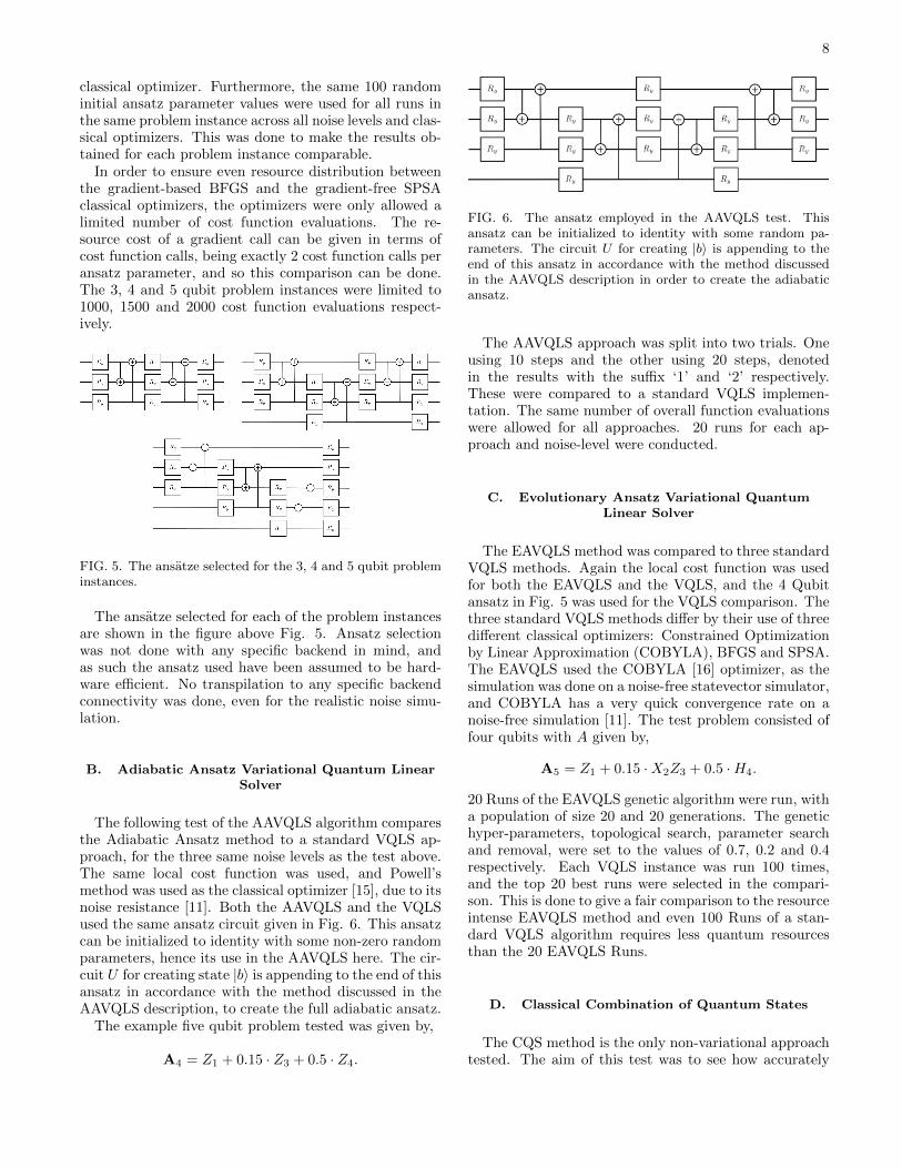
FIG. 5. The ansatze selected for the 3, 4 and 5 qubit probleminstances.

The ansatze selected for each of the problem instancesare shown in the figure above Fig. 5. Ansatz selectionwas not done with any specific backend in mind, andas such the ansatz used have been assumed to be hard-ware efficient. No transpilation to any specific backendconnectivity was done, even for the realistic noise simu-lation.

B. Adiabatic Ansatz Variational Quantum LinearSolver

The following test of the AAVQLS algorithm comparesthe Adiabatic Ansatz method to a standard VQLS ap-proach, for the three same noise levels as the test above.The same local cost function was used, and Powell’smethod was used as the classical optimizer [15], due to itsnoise resistance [11]. Both the AAVQLS and the VQLSused the same ansatz circuit given in Fig. 6. This ansatzcan be initialized to identity with some non-zero randomparameters, hence its use in the AAVQLS here. The cir-cuit U for creating state |b〉 is appending to the end of thisansatz in accordance with the method discussed in theAAVQLS description, to create the full adiabatic ansatz.

The example five qubit problem tested was given by,

A4 = Z1 + 0.15 · Z3 + 0.5 · Z4.

FIG. 6. The ansatz employed in the AAVQLS test. Thisansatz can be initialized to identity with some random pa-rameters. The circuit U for creating |b〉 is appending to theend of this ansatz in accordance with the method discussedin the AAVQLS description in order to create the adiabaticansatz.

The AAVQLS approach was split into two trials. Oneusing 10 steps and the other using 20 steps, denotedin the results with the suffix ‘1’ and ‘2’ respectively.These were compared to a standard VQLS implemen-tation. The same number of overall function evaluationswere allowed for all approaches. 20 runs for each ap-proach and noise-level were conducted.

C. Evolutionary Ansatz Variational QuantumLinear Solver

The EAVQLS method was compared to three standardVQLS methods. Again the local cost function was usedfor both the EAVQLS and the VQLS, and the 4 Qubitansatz in Fig. 5 was used for the VQLS comparison. Thethree standard VQLS methods differ by their use of threedifferent classical optimizers: Constrained Optimizationby Linear Approximation (COBYLA), BFGS and SPSA.The EAVQLS used the COBYLA [16] optimizer, as thesimulation was done on a noise-free statevector simulator,and COBYLA has a very quick convergence rate on anoise-free simulation [11]. The test problem consisted offour qubits with A given by,

A5 = Z1 + 0.15 ·X2Z3 + 0.5 ·H4.

20 Runs of the EAVQLS genetic algorithm were run, witha population of size 20 and 20 generations. The genetichyper-parameters, topological search, parameter searchand removal, were set to the values of 0.7, 0.2 and 0.4respectively. Each VQLS instance was run 100 times,and the top 20 best runs were selected in the compari-son. This is done to give a fair comparison to the resourceintense EAVQLS method and even 100 Runs of a stan-dard VQLS algorithm requires less quantum resourcesthan the 20 EAVQLS Runs.

D. Classical Combination of Quantum States

The CQS method is the only non-variational approachtested. The aim of this test was to see how accurately

9

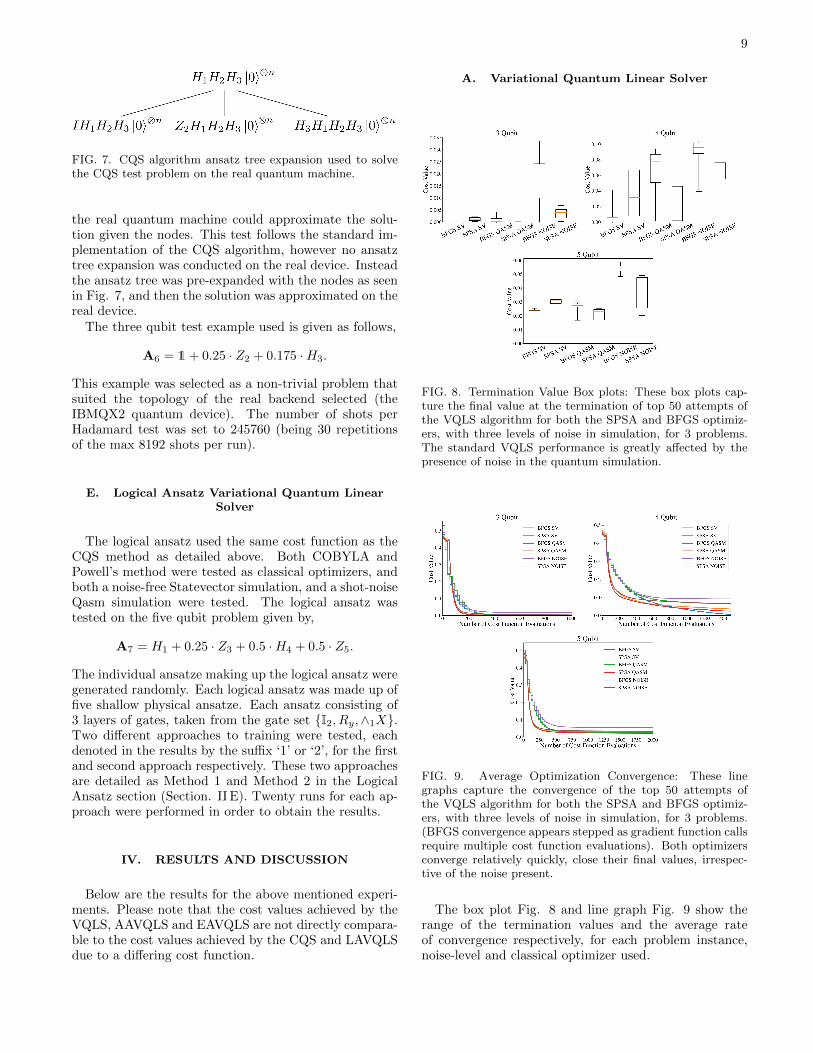
FIG. 7. CQS algorithm ansatz tree expansion used to solvethe CQS test problem on the real quantum machine.

the real quantum machine could approximate the solu-tion given the nodes. This test follows the standard im-plementation of the CQS algorithm, however no ansatztree expansion was conducted on the real device. Insteadthe ansatz tree was pre-expanded with the nodes as seenin Fig. 7, and then the solution was approximated on thereal device.

The three qubit test example used is given as follows,

A6 = 1+ 0.25 · Z2 + 0.175 ·H3.

This example was selected as a non-trivial problem thatsuited the topology of the real backend selected (theIBMQX2 quantum device). The number of shots perHadamard test was set to 245760 (being 30 repetitionsof the max 8192 shots per run).

E. Logical Ansatz Variational Quantum LinearSolver

The logical ansatz used the same cost function as theCQS method as detailed above. Both COBYLA andPowell’s method were tested as classical optimizers, andboth a noise-free Statevector simulation, and a shot-noiseQasm simulation were tested. The logical ansatz wastested on the five qubit problem given by,

A7 = H1 + 0.25 · Z3 + 0.5 ·H4 + 0.5 · Z5.

The individual ansatze making up the logical ansatz weregenerated randomly. Each logical ansatz was made up offive shallow physical ansatze. Each ansatz consisting of3 layers of gates, taken from the gate set {I2, Ry,∧1X}.Two different approaches to training were tested, eachdenoted in the results by the suffix ‘1’ or ‘2’, for the firstand second approach respectively. These two approachesare detailed as Method 1 and Method 2 in the LogicalAnsatz section (Section. II E). Twenty runs for each ap-proach were performed in order to obtain the results.

IV. RESULTS AND DISCUSSION

Below are the results for the above mentioned experi-ments. Please note that the cost values achieved by theVQLS, AAVQLS and EAVQLS are not directly compara-ble to the cost values achieved by the CQS and LAVQLSdue to a differing cost function.

A. Variational Quantum Linear Solver

FIG. 8. Termination Value Box plots: These box plots cap-ture the final value at the termination of top 50 attempts ofthe VQLS algorithm for both the SPSA and BFGS optimiz-ers, with three levels of noise in simulation, for 3 problems.The standard VQLS performance is greatly affected by thepresence of noise in the quantum simulation.

FIG. 9. Average Optimization Convergence: These linegraphs capture the convergence of the top 50 attempts ofthe VQLS algorithm for both the SPSA and BFGS optimiz-ers, with three levels of noise in simulation, for 3 problems.(BFGS convergence appears stepped as gradient function callsrequire multiple cost function evaluations). Both optimizersconverge relatively quickly, close their final values, irrespec-tive of the noise present.

The box plot Fig. 8 and line graph Fig. 9 show therange of the termination values and the average rateof convergence respectively, for each problem instance,noise-level and classical optimizer used.

10

Fig. 8 gives an idea of the difficulty of each probleminstance, and also gives an idea as to the overall affect ofnoise on the optimization process. The 4 qubit probleminstance appears to have been the most difficult, nextbeing the 5 qubit instance, with the 3 qubit instancebeing the simplest to solve.

The VQLS algorithm performs very well in a noise-freestate vector simulation, with the gradient-based BFGSundoubtedly performing the best outright. The inclusionof shot-noise alone does not appear to greatly disturb theoptimization process much, however BFGS is much moreaffected by the shot-noise than the gradient-free SPSA.SPSA very much outperforms BFGS in the presence ofnoise. The realistic noise levels appear to greatly affectthe optimization process, and while again, SPSA is lessaffected than BFGS, both are heavily set back. Thesetrends seen between the different noise levels and classi-cal optimizers appear to hold regardless of the probleminstances apparent difficulty.

Fig. 9 shows the average convergence rate of the top50 attempts, for each noise-level, classical optimizer andproblem instance. In all, SPSA converges faster thanBFGS regardless of noise-level, and the more difficult theproblem, the slower the rate of convergence.

B. Adiabatic Ansatz Variational Quantum LinearSolver

FIG. 10. AAVQLS Termination Values: AAVQLS termina-tion values compared to a standard VQLS approach, for 2different AAVQLS methods for 3 noise levels. These resultsappear to indicate there is not much of a significant differencebetween the VQLS and both AAVQLS approaches.

The box plot Fig. 10 shows the range of the final ter-mination values achieved by the respective methods forthe respective levels of noise.

The line graph Fig. 11 shows an average value of thecost function along the adiabatic optimization path for

FIG. 11. Average Optimization Convergence: These linegraphs capture the cost value measured by the AAVQLS algo-rithm during the optimization process, for 2 different meth-ods, for 3 noise levels. This corresponds to how close theansatz kept to the ground state of the Hamiltonian duringthe optimization.

the best performing run of both AAVQLS 1 and 2 foreach noise level.

The results captured in Fig. 10 appear to indicatethere is not much of a significant difference betweenthe VQLS and both AAVQLS approaches. However,the state vector simulation clearly favours the standardVQLS approach, while the both AAVQLS approachesslightly outperform the VQLS in the realistic noise situ-ation. Given that the state vector simulation is merelytheoretical, there may be some merit to the AAVQLSapproach. AAVQLS 2 also ever so slightly outperformsAAVQLS 1 in the noisy simulations, meaning shorter,more frequent steps may be the better approach betweenthe two. (The AAVQLS approach was split into two tri-als. One using 10 steps and the other using 20 steps,denoted in the results with the suffix ‘1’ and ‘2’ respec-tively)

The line graph Fig. 11 shows that all methods keptfairly close to the ground state of the Hamiltonian dur-ing the initial phase of optimization, only to move furtheraway from the ground state during the middle of the opti-mization process. The Statevector and Qasm simulationsof both methods managed to move close to the groundstate near the end of the optimization process howeverthe noisy simulations did not. Ideally all methods shouldhave kept fairly close to the ground state throughout theoptimization process.

C. Evolutionary Ansatz Variational QuantumLinear Solver

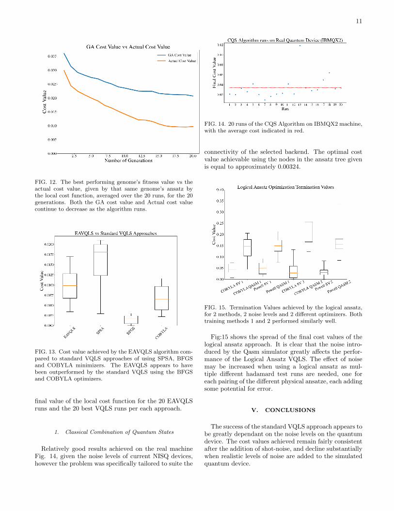
The line graph Fig. 12, shows the difference betweenthe best genome’s fitness value (discussed in EAVQLSsection) and the actual local cost function value per gen-eration averaged across the 20 runs.

The box plot Fig. 13 shows the difference between the

11

FIG. 12. The best performing genome’s fitness value vs theactual cost value, given by that same genome’s ansatz bythe local cost function, averaged over the 20 runs, for the 20generations. Both the GA cost value and Actual cost valuecontinue to decrease as the algorithm runs.

FIG. 13. Cost value achieved by the EAVQLS algorithm com-pared to standard VQLS approaches of using SPSA, BFGSand COBYLA minimizers. The EAVQLS appears to havebeen outperformed by the standard VQLS using the BFGSand COBYLA optimizers.

final value of the local cost function for the 20 EAVQLSruns and the 20 best VQLS runs per each approach.

1. Classical Combination of Quantum States

Relatively good results achieved on the real machineFig. 14, given the noise levels of current NISQ devices,however the problem was specifically tailored to suite the

FIG. 14. 20 runs of the CQS Algorithm on IBMQX2 machine,with the average cost indicated in red.

connectivity of the selected backend. The optimal costvalue achievable using the nodes in the ansatz tree givenis equal to approximately 0.00324.

FIG. 15. Termination Values achieved by the logical ansatz,for 2 methods, 2 noise levels and 2 different optimizers. Bothtraining methods 1 and 2 performed similarly well.

Fig:15 shows the spread of the final cost values of thelogical ansatz approach. It is clear that the noise intro-duced by the Qasm simulator greatly affects the perfor-mance of the Logical Ansatz VQLS. The effect of noisemay be increased when using a logical ansatz as mul-tiple different hadamard test runs are needed, one foreach pairing of the different physical ansatze, each addingsome potential for error.

V. CONCLUSIONS

The success of the standard VQLS approach appears tobe greatly dependant on the noise levels on the quantumdevice. The cost values achieved remain fairly consistentafter the addition of shot-noise, and decline substantiallywhen realistic levels of noise are added to the simulatedquantum device.

12

The AAVQLS approach presents an ansatz optimiza-tion strategy that in theory could keep the ansatz nearthe ground state of the system’s Hamiltonian, allowing alow cost value to be easily found. Considering the bestruns recorded in Fig. 11, this trend is observed duringthe first part of the optimization where at all levels ofnoise, the system remained close the the ground state ofthe Hamiltonian. This trend faded just before midwaythrough the optimization process, where all simulations,regardless of the level of noise, moved away from theground state. This presents a particular flaw in this ap-proach, whereby the system can leave the ground state.One possible explanation for this is that the optimizationprocess had a step size that was too large (the evolutionof the Hamiltonian was too fast), or the ground statewas not contained in the Hilbert space spanned by theparticular ansatz used. The latter issue may be avoidedby evolving the initial Hamiltonian to the final Hamilto-nian along a different path. In the later half of the opti-mization process, the Statevector and QASM simulationsrecovered the ground state while the realistic noise sim-ulation did not. That the AAVQLS performs similarlyto the VQLS in the QASM and Noisy simulations, asseen in Fig. 10, suggests that there may be some meritto this approach, especially because the best cost val-ues achieved by the AAVQLS for those two simulationswere quite substantially lower, even if, on average, theyperformed similarly.

The EAVQLS performed at around the same level asthe VQLS for the specific problem instance simulated inthese results. Seeing as only a statevector simulation wasconducted, it is not yet known how a noisy simulationmay have changed these results, as a key selling point ofthe EAVQLS algorithm is noise resistance, due to shorter,more problem and hardware specific ansatze.

The CQS approach was the only approach tested onthe real quantum device, in order to gauge its effective-ness on near-term quantum hardware. With 20 runs

on the IBMQX2 device, the CQS approach managed toachieve some fairly low cost values and a decent averagecost value. This is positive for this approach, however itis noted that the specific problem that was solved mayhave been quite simple, yet still non-trivial.

The LAVQLS, being an adaptation of the CQSmethod, appears to work well in a noise-free simulation,however the shot-noise alone heavily reduced the finalcost value achieved by the method. This may be be-cause the many hadamard tests required to evaluate thecost function amplify the noise. This is not good becausea proposed feature of the LAVQLS was noise resistancedue to the use of shorter individual ansaze making up thelogical ansatz.

In this paper a few approaches to solving systems oflinear equations on near-term quantum hardware havebeen presented. Each approach that differs from thestandard VQLS approach tries to offer some advantageover the standard approach, however whether the pro-posed advantages of these algorithms actually apply inimplementation is yet to be conclusively seen. Some po-tential problems with these approaches have been high-lighted and it is left to a future work to investigate therealistic advantages of these approaches. It may be thecase that some of these approaches offer significant ad-vantages over the standard VQLS approach, however thisis still unclear.

ACKNOWLEDGMENTS

This work is based upon research supported by theSouth African Research Chair Initiative, Grant No.64812 of the Department of Science and Innovation andthe National Research Foundation of the Republic ofSouth Africa. Support from the NICIS (National In-tegrated Cyber Infrastructure System) e-research grantQICSA is kindly acknowledged.

[1] Aram W. Harrow, Avinatan Hassidim and Seth Lloyd,“Quantum algorithm for linear systems of equations,”Phys. Rev. Lett., Vol 15, No. 103, Pp. 150502 (2009)

[2] Danial Dervovic, Mark Herbster, Peter Mountney, Si-mone Severini, Naıri Usher and Leonard Wossnig,“Quantum linear systems algorithms: a primer” (2018)arXiv:1802.08227

[3] John Preskill, “Quantum Computing in the NISQ eraand beyond”, Quantum 2, Vol. 79 (2018)

[4] Jarrod R. McClean, Sergio Boixo, Vadim N. Smelyanskiy,Ryan Babbush, and Hartmut Neven, “Barren plateausin quantum neural network training landscapes”, NatureCommunications, 9:4812 (2018)

[5] Alberto Peruzzo, Jarrod McClean, Peter Shadbolt, Man-Hong Yung, Xiao-Qi Zhou, Peter J. Love, Alan Aspuru-Guzik and Jeremy L. O’Brien, “A variational eigenvaluesolver on a quantum processor”, Nature Communica-tions, 5:4213 (2014)

[6] Carlos Bravo-Prieto, Ryan LaRose, M. Cerezo, YigitSubası, Lukasz Cincio and Patrick J. Coles, “VariationalQuantum Linear Solver: A Hybrid Algorithm for LinearSystems” (2019) arXiv:1909.05820

[7] Hsin-Yuan Huang, Kishor Bharti and Patrick Reben-trost, “Near-term quantum algorithms for linear systemsof equations” (2019) arXiv:1909.07344

[8] William J. Huggins, Joonho Lee, Unpil Baek, BryanO’Gorman and K Birgitti Whaley, “A non-orthogonalvariational quantum eigensoler”, New Journal of Physics,22, 073009 (2020)

[9] Arthur G. Rattew, Shaohan Hu, Marco Pistoia, RichardChen and Steve Wood, “A Domain-agnostic, Noise-resistant, Hardware-efficient Evolutionary VariationalQuantum Eigensolver” (2020) arXiv:1910.09694

[10] K. Mitarai, M. Negoro, M. Kitagawa and K. Fujii,“Quantum Circuit Learning,” Phys. Rev. A 98, 032309(2019)

13

[11] Aidan Pellow-Jarman, Ilya Sinayskiy, Anban Pillay andFrancesco Petruccione, “A comparison of various classi-cal optimizers for a variational quantum linear solver”,Quantum Information Processing, 20, 202 (2021)

[12] Tameem Albash, Daniel A. Lidar, “Adiabatic QuantumComputing”, Rev. Mod. Phys 90, 015002 (2018)

[13] R. Fletcher, “A new approach to variable metric al-gorithms,” The Computer Journal, Vol. 13, Iss. 3, Pp317–322 (1970)

[14] J. C. Spall. “Multivariate Stochastic Approximation Us-ing a Simultaneous Perturbation Gradient Approxima-

tion,” IEEE Transactions on Automatic Control, Vol. 37,No. 3, Pp. 332–341, (1992)

[15] M. J. D. Powell, “An efficient method for finding theminimum of a function of several variables without cal-culating derivatives,” Computer Journal, Vol. 7, Iss. 2,Pp. 155–162 (1964)

[16] M. J. D. Powell, “A direct search optimization methodthat models the objective and constraint functions bylinear interpolation,” Advances in Optimization and Nu-merical Analysis, Pp. 51-67 (1994)