near infrared microsensor for continuous in-vivo - deep blue
TRANSCRIPT
Near Infrared Microsensor for Continuous In-vivo Intraocular and Intracranial Pressure Monitoring
by
Mostafa Ghannad-Rezaie
A dissertation submitted in partial fulfillment of the requirements for the degree of
Doctor of Philosophy (Biomedical Engineering)
in the University of Michigan
2013
Doctoral Committee: Associate Professor Nikolaos Chronis, Chair Assistant Professor Jianping Fu Professor Edgar Meyhofer Professor Shuichi Takayama Associate Professor Lynda Jun-San Yang

ii
To My Family

iii
Table of Contents
Dedication..................................................................................................................................................... ii
List of Figures ............................................................................................................................................... vi
List of Tables ................................................................................................................................................ xii
Abbreviation ............................................................................................................................................... xiii
Abstract ...................................................................................................................................................... xiv
CHAPTER
1. INTRODUCTION ....................................................................................................................................... 1
1.1 Motivation ........................................................................................................................................... 1
1.1.1. Axonal Injury and Active Response to Mechanical Stimulation ................................................. 2
1.1.2. Model Organism for Single Neuron Study .................................................................................. 4
1.1.3. Mammalian Model of Injury and Clinical Requirements .......................................................... 7
1.2. Thesis Objective ................................................................................................................................. 8
1.3. Thesis Organization ............................................................................................................................ 9
2. IN-VIVO MECHANICAL STRESS ASSAY: DROSOPHILA LARVA ON MICROFLUIDIC CHIPS ..................... 12
2.1. Introduction ..................................................................................................................................... 13
2.2. In-vivo Imaging of Cellular Responses to Neural Injury .................................................................. 15
2.3. Single Injury Response and Chronic Pressure Effect ........................................................................ 18
2.3.1. The SI and LI microfluidic larva chips ........................................................................................ 18
2.3.2. On-chip calcium imaging within milliseconds of injury. ........................................................... 22
2.3.3. Monitoring changes in axonal transport after injury.. .............................................................. 23
2.3.4. Long-term, time-lapse imaging of axonal sprouting after injury.. ............................................ 27
iv
2.4. Discussion and Summery ................................................................................................................. 27
2.4.1 The SI and LI chips for Drosophila larva immobilization. ........................................................... 30
2.4.2. The SI chip allows for in-vivo imaging of neural activity.. ......................................................... 31
2.4.3. The larva chips allow monitoring of rapid changes in axonal transport. .................................. 31
2.4.4. Studying regenerative responses on-chip.. .............................................................................. 32
2.4.5. The LI chip allows for in vivo mechanical stimulation.. ............................................................ 33
3. OPTO-MECHANICAL MICROSENSOR FOR INTRACRANIAL PRESSURE MONITORING .......................... 36
3.1.Introduction ...................................................................................................................................... 37
3.2.NiFO Sensing Technology ................................................................................................................. 40
3.2.1. Sensor Architecture .................................................................................................................. 41
3.2.2. Microfabrication Process .......................................................................................................... 43
3.3. Results and Discussion ..................................................................................................................... 44
3.3.1. Membrane Deflection Versus Pressure ................................................................................... 44
3.3.2. Intensity Ratio versus Pressure. ............................................................................................... 45
3.3.3. Maximum Error ........................................................................................................................ 50
3.3.4. Drift and Photostability of the NiFO sensor .............................................................................. 52
3.3.5. ‘Zero-Misalignment’ Pressure .................................................................................................. 56
3.3.6. Effect of Skin on the performance of the NiFO sensor ............................................................. 57
3.4.Summary .......................................................................................................................................... 60
4. IMPLANTABLE INTRAOCULAR PRESSURE SENSOR: EX VIVO STUDIES ................................................. 62
4.1. Introduction ..................................................................................................................................... 62
4.2. Method ............................................................................................................................................ 64
4.2.1. Design and fabrication .............................................................................................................. 64
4.2.2. Keratoprosthesis implantation ................................................................................................ 65
4.3. Results .............................................................................................................................................. 71
4.4. Discussion and Summary ................................................................................................................. 73
5. IN-VIVO IMPLANTATION OF OPTICAL SENSOR IN SHEEP MODEL ....................................................... 78
5.1. Introduction ..................................................................................................................................... 78

v
5.2. Sensor Implantation Method ........................................................................................................... 79
5.2.1. NiFO Sensor and ICP Express Calibration .................................................................................. 80
5.2.2. Cranial Access ........................................................................................................................... 80
5.2.3. measuring Intracranial measurement ...................................................................................... 82
5.2.3. Closing the incision ................................................................................................................... 82
5.2.4. Testing the dynamic range of microsensor in vivo ................................................................... 82
5.3. Results and Discussions .................................................................................................................... 84
5.3.1 Comparing Codman and NiFO sensors ...................................................................................... 84
5.3.2 NiFO signal to noise ratio ........................................................................................................... 88
5.4. Summery .......................................................................................................................................... 88
6. CONCLUSIONS AND FUTURE WORK ..................................................................................................... 90
6.1. Conclusion ........................................................................................................................................ 90
6.1.1. Single Cell Model to Study Neuronal Injury .................................................................................. 91
6.1.2. NiFO Technology to Study Injury Response to Mechanical Stress in ........................................... 91
6.2. Future Works.................................................................................................................................... 92
6.2.1. Fabry-Perot Laser Cavity Pressure Sensor Technology ............................................................. 92
6.2.2. Long-term experiments and Validate that the NiFO sensors ................................................... 95
6.2.3. Regulation path and biocompatibility ...................................................................................... 96
Bibliography................................................................................................................................................ 98
vi
List of Figures
Figure 1.1. Axonal injury timeline: A. axonal injury stages caused by acute mechanical stress. B. Timeline of axonal degeneration and regeneration in Drosophila larva……………………………………..6
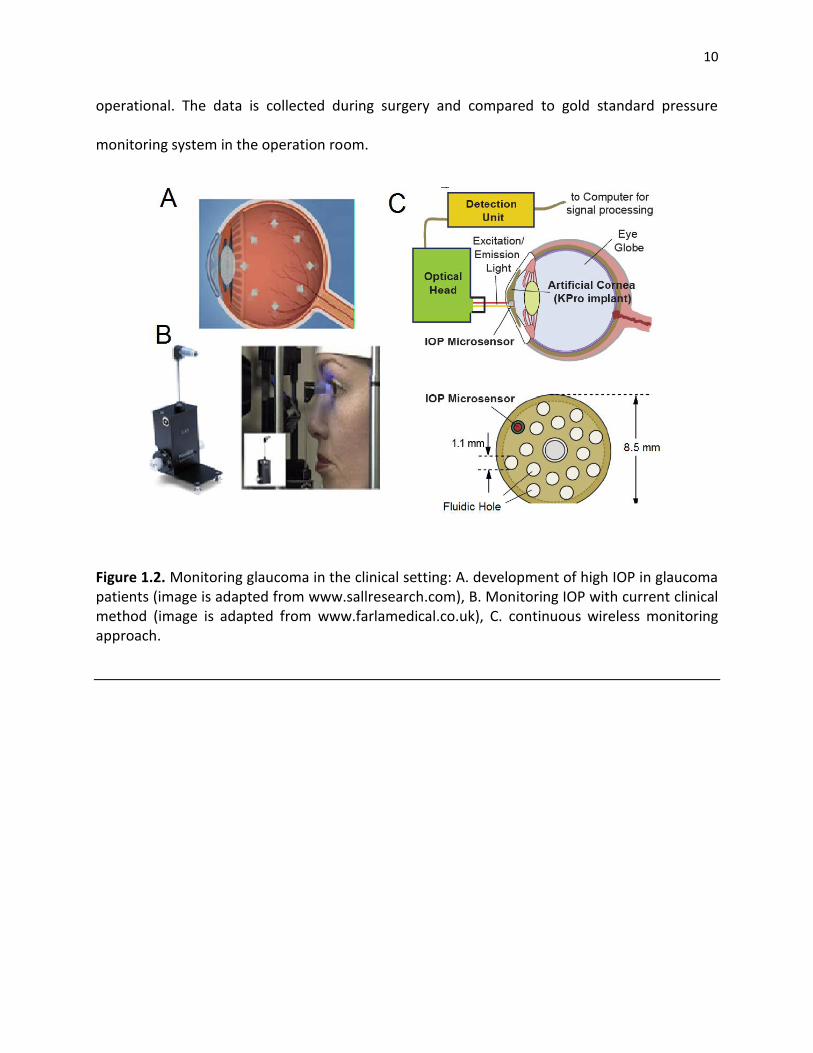
Figure 1.2. Monitoring glaucoma in the clinical setting: A. development of high IOP in glaucoma patients, B. Monitoring IOP with current clinical method, C. continuous wireless monitoring approach………………………………………………………………………………………………………………………………….10
Figure 1.3. Monitoring TBI in the clinical setting: A. development of high ICP in TBI, B. Monitoring ICP with current clinical method, C. implantation of catheter for ICP monitoring, D. continuous wireless monitoring approach……………………………………………………………………………….11
Figure 2.1. The SI and LI microfluidic chips for immobilizing Drosophila larva. (A) the SI-chip is a single-layer PDMS microfluidic device that utilizes a shallow (140 µm thick) immobilization microchamber to squeeze larvae in the vertical direction. Scale bar, 1 mm. (B) the two-layer LI-chip. The first PDMS layer (labeled with blue color) has the larva immobilization microchamber and is connected to two microfluidic channels to supply food to the larva head (typically delivered every 30 min). A second PDMS layer (labeled with red color) is vertically integrated into the first PDMS layer to deliver CO2 through a 10-µm thick PDMS membrane. In both the SI and LI chips, a microfluidic network surrounding the immobilization chamber is used to create a tight seal between the PDMS and the glass coverslip. Scale bar, 1 mm. (C) (I) Bright-field image of a 3rd instar larva immobilized in the LI-chip. Scale bar, 1 mm. (II) Fluorescent images of the larva body (highlighted in the red square in C(I)) before (top image) and after (bottom image) immobilization. After application of CO2 at 5 psi, the larva is immobilized and the GFP-labeled ventral nerve cord is brought into focus (bottom image). Scale bar, 20µm………………………………19
Figure 2.2. Survival rates and body movement of on-chip immobilized larvae. (A) Survival rate of continuously immobilized larvae using the SI-chip. Five different immobilization microchambers thicknesses were tested. We considered a thickness of 140 µm (red curve) to be optimal, as thicknesses higher than 140 µm resulted in poor immobilization. (B) Survival rates on the LI-chip using periodic immobilization (30 s of immobilization every 5 min). We considered a thickness of 170 µm (red curve) to be optimal as more than 85% of larvae survived the immobilization
vii
procedure after 10 hours. (C) Average larva body movement using the LI-chip for different thicknesses of the immobilization microchamber (30 s of immobilization every 5 min). In all plots, error bars represent standard error of the mean obtained from 10 larvae…………………….20
Figure 2.3: Recovery after immobilization. Animals are immobilized for 30 seconds under different conditions. The body movement, first the animal is imaged (5 frame/sec). The movement between frames was calculated using a fast block matching algorithm.The body movement is recorded over a time course from 15 seconds before immobilization to 50 seconds after immobilization. To measure The red line represents the average body movement of 10 samples. The grey lines represents average movement recorded from 10 larva. The dashed line indicates the time of immobilization. (A) After immobilization with pressure alone (5 psi air pressure, 30 seconds), larvae regain full mobility within 10 seconds. (B) After immobilization with 95/5% CO2/air, the larvae regain full motility within 30 seconds after releasing the pressure. (C) Larvae were immobilized every 5 minutes for 10 hours in the LI-chip, and then assayed for recovery after 30 seconds of immobilization with 95/5% CO2/air. The larvae still recover within 30 seconds, similarly to (B)……………………………………………………………………………….22
Figure 2.4. Diagram of neurons and Gal4 drivers. (A) Class IV sensory neurons (blue), labeled by ppk-Gal4, were used to study the Ca2+ responses to laser ablation of a dendrite (in Figure 2) because both their cell bodies and dendrites lie close the cuticle, allowing for excellent reproducible injury by the pulsed dye laser, and excellent visualization of cellular responses close to injury site. B) The eve(RRa)Gal4 driver expresses specifically in aCC and RP2 motneurons (green). These were used for the study of axonal transport after nerve crush injury (in Figure 3) because the regenerative response to injury has been previously characterized in these neurons. (C) The RN2-Gal4 driver line, which labels enteric motoneurons in larvae (red), was used for the time lapse study of regeneration. This driver line is very strong, allowing for both UAS-GMA and UAS-mCD8-RFP to be expressed at high levels. While these neurons display similar reactions to both laser axotomy and nerve crush, we focused upon laser axotomy for Figure 4 because this injury is small enough to fit within one field of view……………………………..25
Figure 2.5. Calcium dynamics after laser axotomy. (A) Time-lapse images from immobilized larvae depict intracellular calcium dynamics during laser microsurgery. Sensory neurons expressing G-CaMP and GFP were ablated with a pulsed UV laser (see also supplementary movies 1 and 2). (B) Average normalized fluorescent intensity (ΔF/F0) from G-CaMP and GFP expressing neural cell bodies (sample size, n = 12) before and after injury (injury is performed at 0 sec). A peak value in the intensity of G-CaMP is observed 2 seconds after injury. Calcium transients from individual larvae are depicted in light grey color. (C) Quantification of the maximum fluorescent intensity change (maximum ΔF/F0). The fluorescent intensity from GFP expressing neurons did not change significantly (p-value < 0.01, n =12)…………………………………26
Figure 2.6. Changes in axonal transport after nerve-crush injury. (A) Kymographs of ANF-GFP labeled vesicles in an uninjured axon, and 3 hours after injury in the distal stump and proximal stump. (B) Particle density (anterograde, retrograde, and stationary) was quantified per 100 µm of axon length. In the proximal stump 3 hours after injury, there was a 90% increase in anterograde particle density (p-value = 0.03, n = 16), but no significant change in retrograde
viii
particle density (p-value < 0.01, n = 16). In contrast, transport was almost completely halted in the distal stump (p value < 0.01, n = 8). Error bars represent standard error of the mean…….27
Figure 2.7. ANF-GFP particle density for on-chip immobilized and flay-open larvae. In the flay-open protocol, 3rd instar larvae were quickly dissected, mounted between a coverslip and a glass-slide and imaged within 5 min after dissection. Particles from 10 axons and 24 axons were analyzed using the on-chip and flay-open methods respectively. No significant differences between the two methods were observed (p-value < 0.01)……………………………………………………28
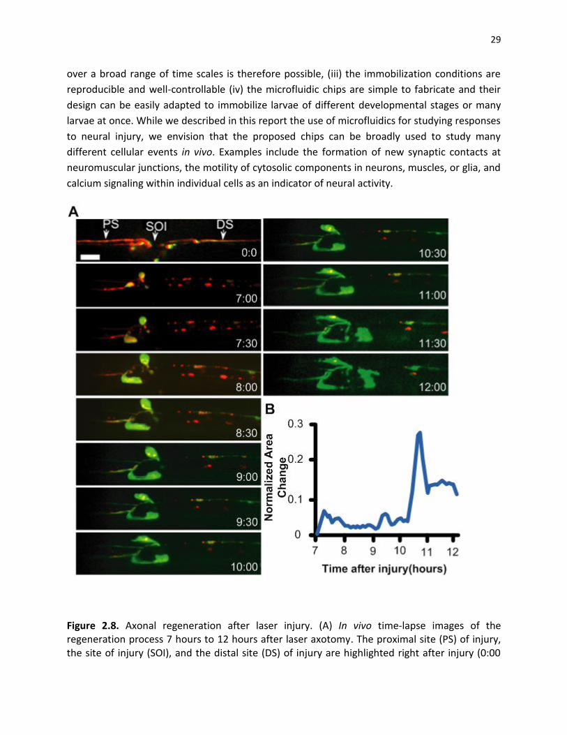
Figure 2.8. Axonal regeneration after laser injury. (A) In vivo time-lapse images of the regeneration process 7 hours to 12 hours after laser axotomy. The proximal site (PS) of injury, the site of injury (SOI), and the distal site (DS) of injury are highlighted right after injury (0:00 frame). The red color represents RFP expression that is localized in the membrane of the axon. The green color represents F-actin expression. Scale bar, 10 µm. (b) Normalized area change of the proximal stump over time. Significant movement in the proximal stump is observed ~10.5 hours after injury.........................................................................................................................29 Figure 2.9. On-chip axon regeneration after laser axotomy. (a) In vivo time-lapse images of the proximal site (PS) of injury, the site of injury (SOI), and the distal site (DS) of injury, 10 hours after laser axotomy. The red color represents red fluorescent protein (RFP) expressed in the membrane of the axon. The green color represents F-actin. Scale bar, 10 µm. (b) Normalized area change of the proximal stump between 10 and 11 hours after injury.................................30
Figure 2.10. ANF-GFP particle density for on-chip for different pressure patterns. A. Particles from 10 axons and 24 axons were analyzed using the on-chip control, low and high frequency of change in the pressure respectively. No significant differences between the low frequency of immobilization and control were observed (p-value < 0.01). However, in the variable pressure scenario, the stationary particle density increases significantly. B. the degeneration is observed for high frequency of high pressure. C. the frequency that pressure applied and D. the temporal pattern of pressure (speed of rising and falling of pressure) is more important factor regulating the axonal transport speed ................................................................................................................................ 33
Figure 2.11. Effect of frequency and pressure level on the survival of neurons. A. Particles from 10 axons and 24 axons were analyzed using the on-chip control, low and high frequency of change in the pressure respectively.The survival rate is analyzied in different pressure levels .............................. 34
Figure 3.1. (A) The NiFO technology. The external optical readout unit is used to collect spectroscopic data from the implanted NiFO sensor in the near infrared (NI). (B) Cross sectional view of the NiFO sensor. (C) The working principle of the ICP sensor. (D) The microfabricated device sitting on a penny. Chip III has been removed to illustrate the presence of the mini-lens. A 1.6 mm x 1.6 mm silicon nitride membrane with a patterned QD micropillar is shown in the inset. Scale bar, 1 mm .............................................................................................................................. 39
ix
Figure 3.2. Normalized fluorescence spectrum emitted by the QD micropillar versus applied pressure. At zero pressure, the 705 nm QD layer is in focus. As pressure increases, the 800 nm QD layer comes in focus as indicated by the increased intensity near that wavelength. The 705 nm and 800 nm QD layers show a maximum peak at 695 nm and 790 nm respectively. That shift can be attributed to the photooxidation of the QDs. The shadowed areas represent the spectral windows that were used to calculate the average intensity for each QD layer .............................. 41
Figure 3.3. The NiFO sensor consists of three chips, manually assembled on top of each other. Each chip has a transparent, 300 nm thick silicon nitride membrane. The key element of the design, the QD micropillar, consists of two QD layers and two SU-8 layers that are photolithographically patterned on top of the ICP-exposed membrane of wafer I ....................... 43
Figure 3.4. Maximum membrane deflection versus applied pressure for square membranes of 5 different dimensions (0. 8 mm x 0.8 mm, 1 mm x 1 mm, 1.2 mm x 1.2 mm, 1.4 mm × 1.4 mm and 1.6mm x 1.6mm). Error bars represent standard error of the mean (SEM) from 5 measurements (taken from one device). The dotted lines illustrate modeling results ................ 46
Figure 3.5. Schematic of the experimental setup for characterizing the NiFO sensor. The back side of the sensor (chip I) is connected via a plastic tubing to a water column. A similar setup was used to obtain the ‘zero-misalignment’ pressure ........................................................................ 48
Figure 3.6. (A) Representative intensity ratio curve for a NiFO sensor consisting of a 1.4 mm x 1.4 mm square membrane. The fluorescent intensity obtained from each QD layer is also illustrated on the right axis. Error bars represent SEM from 5 measurements (taken from one device). (B) Normalized intensity ratio versus applied pressure for sensors having membranes of 5 different dimensions ............................................................................................................................. 49
Figure 3.7. Percentage precision error (Ep) versus applied pressure. Each Ep value is calculated from 5 measurements taken from a single device (the average of these measurements is depicted in figure 6B). The dotted line illustrates the maximum error set by the Association for the Advancement of Medical Instrumentation (AAMI) for ICP sensors. Large membranes (e.g. the 1.4 mm × 1.4 mm and 1.6mm × 1.6 mm ones) meet the AAMI standards almost through the entire pressure range .............................................................................................................................. 52
Figure 3.8. Measuring drift: three devices with a 1.4 mm x 1.4 mm membrane were kept in distilled water for three weeks under a constant pressure of (A) 20 mmHg and (B) 40 mmHg. The intensity ratio was recorded every three days from each device. No drift was observed ..... 55
Figure 3.9. QD fluorescent intensity versus exposure time. Individual 705 nm and 800 nm QD layers were patterned on a silicon nitride membrane and were continuously exposed with a red (658 nm) laser for more than 3 hours at a power density of 0.75 W/cm2. Despite the initial increase in the intensity in both QD layers, the ratio remained constant (peak-to-peak value was less than 2% over 200 minutes of continuous exposure) .................................................................. 57
Figure 3.10. (A) An optical model for quantifying the effect of skin on the performance of the NiFO sensor. The pseudocolor images illustrate the intensity distribution of a 658 nm laser
x
beam reaching the NiFO sensor. (B) Mont Carlo simulation results depict strong dependence of the skin thickness on the collimated and total (scattered and collimated) light intensity emitted by a 705 nm QD layer .............................................................................................................................. 59
Figure 4.1. The IOP microsensor, A. The integration of optical microsensor into a keratoprosthesis implant B. the operation of microsensor. The nitride membrane deflects when the pressure increases ............................................................................................................................ .63
Figure 4.2. The NiFO sensor consists of a chip, with a micorlens manually assembled on top of
it.The chip has a transparent, 150 nm thick silicon nitride membrane. The key element of the
design, the QD micropillar, consists of two QD layers and two SU8 layers that are
photolithographically patterned on top of the IOP-exposed membrane ........................................ 65
Figure 4.3. A. Ratio between 850nm channel and 920nm verse pressure in mmHg. The ratio is used to calibrate each microsensor separately. B. Simulation result for the membrane with parylene deposition. The simulation suggests 500nm of paraylene deposition change the deflection less than 5% ............................................................................................................................ 66
Figure 4.4. Effect of temperature on the sensor readout: the cadaver eye globe experiment is performed in the room temperature while the in-vivo experiment environment is 37 degree. To make sure the temperature change does not affect the readout, we compare the pressure readout in two settings. In A the chamber pressure is 20mmHg and in B the chamber pressure is 40 mmHg ................................................................................................................................................... 66
Figure 4.5. keratoprosthesis implant, A. the KPro device is consist of 3 parts Back Plate, Locking Ring and Front Part assemble into a Corneal Graft , B. the KPro device assembled with Corneal Graft, C. KPro device after implantation into human globe ............................................................... 68
Figure 4.6. Effect of Parylene deposition on the optical readout of the pressure. To protect the surface of the surface 500nm parylene is deposited in the holder and microsensor. The experimental result should less than 5% change in the calibration curve ...................................... 69
Figure 4.7. A. the microsensor integrated into a KPro implant, B. the keratoprosthesis is implanted into human globe. The location of implant and the microsensor is highlighted with red circles, C. Magnified picture highlighting the location of the microsensor .............................. 71
Figure 4.8. IOP Measurement setup, A. Optical head, B. Digital pressure monitor directly connected to ocular chamber. C. schematic of the setup, the globe is filled with saline solution and the pressure increased to 80mmHg. As pressure decreases the reading from digital sensor is compare to optical head readout form NiFO microsensor ............................................................. 72
Figure 4.9. IOP optical head details: A. the base unit to analysis of light connected to optical head using a fiber optics, B. Optical head equipped by a laser source to active the sensor and collect the QDs signal, C. Ambient light sensor .................................................................................... 74
Figure 4.10. The experimental result for 5 sensors over a week: The globes are filled with saline (the pressure inside the globe is higher than 80mmHg). The digital manometer (M on X axis)

xi
and wireless optical sensor (Optical on Y axis) are recorded simultaneously. As saline leaked out of the globe slowly, the globe pressure drops. The experiment stopped when the pressure is lower than 5mmHg .................................................................................................................................. 75
Figure 5.1. The schematic cross section of sheep brain. A. Axial View, B Sagittal view, C. The top
view of skull and the location of microsensors and Codman sensor. D. The brain picture. The
pressure sensors are placed anterior with respect to motor cortex to avoid cortical structures.
The microsensor is 1 inch deep; the sensor is design to avoid subcortical structure and
ventricles ................................................................................................................................................... 79
Figure 5.2. Candman and NiFO sensor implantation procedure. A. drilling the 4.8 mm hole in
the anterior side of motor neurons, B. drilling parallel holes for Codman sensor, C. end of
procedure with three NiFO sensor and one Codman sensor implantation, D. Closing the skin and
preforming the readout ........................................................................................................................... 81
Figure 5.3. The pressure and oxygen level recording from NiFO sensor over the cross of 2.5 hours of
surgery. A. The recording of pressure readout out of optical head, heart rate and tissue oxygenation, The
red bar represent invasive procedures (closing the jugular arteries and injecting the blood in the brain B.
High-light of different phases of testing the dynamic range of sensor ...................................................... 85
Figure 5.4. The pressure and oxygen level recording from NiFO sensor over the cross of 2.5 hours of
surgery. A. The recording, B. High light of different phases of process, C. auto adjustment of brain in
different stages ........................................................................................................................................... 86
Figure 5.5. comparing average Codman microsensor and optical signal from three NiFO microsensors.
Time is in seconds. The sensors are recorded at discreet time intervals. The new acquisition is
highlighted using a blue arrow. The raw signal from each channel is also shown. The blue window
highlights the acquisition without skin ....................................................................................................... 87
Figure 6.1. FB Cavity laser pressure sensor. A. the cross section of device, B. The fabricated device top view, the scale bar is 300 µm. C. Operational principle of the device. D. The fabrication process of the microsensor. The top and bottom micromirrors are made out of 90 nm and 55 nm thick gold layers respectively. A 10 nm thick chrome layer is used to improve the adhesion. The oxide thickness (~645 nm thick) defines the thickness of the laser cavity ............................................................................................................................ 94
Figure 6.2. A. At 40 mmHg, the lasing wavelength of the microsensor is ~900 nm wavelength. B. Lasing
wavelength versus applied pressure .................................................................................................................... 95

xii
List of Tables
Table 4.1. Standard error correlation between immediate and last readout ................................ 77
Table 4.2. Errors within 0 to 2 mmHg range ....................................................................................... 77 Table 4.3. R factor correlation between immediate and last readout ............................................ 77
Table 5.1. Radiometric measurement of Blood Composition over the surgery and NiFO readout .................................................................................................................................................................... 89
xiii
Abbreviations
CSF Cerebrospinal Fluid FP Fabry-Perot GAT Goldmann applanation tonometer ICP Intracranial Pressure IOP Intraocular Pressure KPro Keratoprosthesis LI Long Term Immobalization NiFO Near Infrared Optio-mechanical PDMS Polydimethylsiloxane MRI Magnetic resonance imaging QD Quantum Dot SI Short-term Immobaliztion
xiv
Abstract
Pressure monitoring in the nervous system is widely used to evaluate therapeutic interventions
in patients with severe pathological elevated pressure in the brain (such as traumatic brain
injuries (TBI) and hydrocephalus) and in the eye (e.g. glaucoma). Monitoring the pressure has
been shown to reduce the number of deaths in TBI patients by 20% and number of blindness in
glaucoma patients by 50%. Continuous, long-term in-vivo pressure monitoring, therefore is a
necessity for planning interventional treatment for the patients in the risk.
The clinical method for monitoring the pressure is not changes in past 40 years. Non-
invasive tonometer for glaucoma patients are inaccurate and cannot be used for continuous
monitoring. Current invasive clinical pressure monitoring practices often employ a catheter
that records the pressure surgically inserted in the brain or in the eye. These catheter-based
systems have been successful so far in accurately monitoring pressure but they are not
appropriate for long-term monitoring as: (i) the patient is continuously connected to the non-
portable monitoring unit, and (ii) the long-term placement of the catheter significantly
increases the risk of infection.
Motivated by the need for frequent, long-term pressure monitoring and the lack of
commercially available fully implantable microsensors, we developed a novel class of MEMS-
based, pressure technology, termed ‘Near infrared Fluorescent-based Optomechanical (NiFO)’
xv
pressure sensing technology. NiFO technology is based on a fully implantable, powerless,
optical microsensor (the NiFO sensor) that converts physiological pressure into a two-
wavelength optical signal in the near infrared (NI) spectrum. NiFO microsensors were
microfabricated using silicon bulk micromachining and were shown to operate at a
physiologically relevant pressure range (0-100mmHg). They have a maximum error of less than
15 % throughout their dynamic range and they are extremely photostable. We adapted the
microsensor design to measure intracranial pressure (ICP) and intraocular pressure (IOP) and
we demonstrated their in-vivo operation for over a month in sheep. We envision that the
proposed NiFO sensing technology will not only help in efficiently managing ICP-elevated
medical conditions, but it will inaugurate a new era in the development of implantable,
electronic and power-free miniaturized devices that can be used in a variety of biomedical
pressure monitoring applications.
1
CHAPTER 1
INTRODUCTION
1.1. Motivation
An important goal of neuroscience is to understand how the neurons sense and respond to
injury. The injury response, either neural regeneration to regain functionality after injury or
degeneration and apoptosis, is regulated through a sophisticated molecular pathway actively
responding to environmental cues including mechanical stress. Long-term recovery from
neurological damage, a complex and delicate process, depends on therapeutic interventions
controlled through monitoring the patient condition closely.
How environmental and physiological conditions affect the response to injury is an
exceptionally important question for devising proper treatment plan [1-4]. Answer to this
question holds the key to the effective treatment of many neurological disorders sharing similar
molecular pathways. Yet, our understanding of pathobiology of neural response to injury is
limited, partially due to lack of continuous long-term patient monitoring capability.
Mechanical stimulation as a major form of environmental cue plays a central role in the
neural injury response regulation. A moderate strain along the neuron is required for
2
directional regeneration; however, elevated pressure for an extended period is shown to
increase morbidity in neurological conditions such as stroke, traumatic brain injury and
glaucoma. Understanding how mechanical stimulation (e.g. pressure) damages neuron
improves the management of neurological disorders involving elevated pressure.
To enhance our understanding the role of elevated pressure in the progress of
neurological conditions, in this work we accomplished following aims: (i). At least in the single
neuron level in a model organism (e.g. Drosophila Larva) we show that continuous pressure
monitoring can potentially change the course of treatment. (ii) Motivated by the need for
frequent long-term pressure monitoring in patients with high risk of neurological disorder, we
developed an implantable microsensor small enough for brain and eye implantation --- two
primary sites for neurological disorders with the risk of elevated pressure. (iii) We performed in-
vivo study to establish the functionality of microsensors and the feasibility of the microsensor
implantation.
1.1.1. Neuronal Damage In Response to Mechanical Stress
Neurons can accommodate a certain degree of mechanical stress. When that threshold is
reached, such as in the case of a spinal cord injury, or of brain hemorrhage where the
intracranial pressure is high, the damage can be irreversible and most likely permanent. In the
former case, the neuronal axon is disrupted and the neuronal connectively is lost. In the latter
case, the increased pressure alters the physiology of the cell body and causing –in extreme
case- neuronal death.

3
(a) Axonal Degeneration. Because axons make long distance connections in central and
peripheral nervous system, they are particularly vulnerable components of neuronal circuit.
Primarily, because they are long, axons are more likely to be damaged during the course of
time. The long distances between the connection sites of axons also inhabit the regeneration
after damage.
In most neural injury the axon segment distal to the injury site are often separated from
the cell body, thus degeneration at the distal end thought to be a passive process, resulting
from a lack of nutrients and support from the cell body (Figure 1.1)[7]. However, the discovery
of a degeneration mechanism known as Wallerian Degeneration [8-10], demonstrates the axon
degeneration is in fact an active process. As distal axons undergo degeneration, the proximal
axons degenerate as in central nervous system (CNS) of human [11] or regenerate as in
invertebrate models such as C. elegans or Drosophila as well as in peripheral nervous system
(PNS) in mammalians [12]. Successful regrowth can reestablish the axonal wiring before distal
degeneration [13] and prevent cell body damage. Both active degeneration and regeneration
mechanism are regulated through molecular pathways not fully understood.
(b) Neuronal Cell body damage. Extensive axonal injury could cause cell body damage and
eventually necrosis [7] and apoptosis [10]. How neuron respond to injury is not only important
for treatment of neural damage, but also for neurodegenerative diseases of which many
involve disconnection and disruption of axons. The mechanisms behind many degenerative
diseases such as Alzheimer’s disease [5] or Parkinson’s disease [6] share the same cellular
degeneration pathway. Similar molecular pathways among neurodegenerative diseases and
4
axonal injuries make the study of axonal injury response even more important. Despite much
effort that has been devoted toward understanding the underlying mechanisms of injury still
very few treatments is known for stroke, traumatic brain injuries, optical nerve damage and
spinal cord injuries.
Much attention is focused on how the environmental factors inhibit neuronal
regeneration [13]. In the absence of the environmental cues all neurons show intrinsic
capability to regenerate. Yet environmental factors are shown to play a significant role in the
active process of regeneration and degeneration [14, 15]. The effect of mechanical pressure, as
an important environmental cue, on the neural injury response was thought to be a passive
process, resulting only from physical restriction of the neuron blood supply. However, the
recent studies in the case of chronic stress show that the neuron senses the mechanical cues
and responds to them through molecular pathways that change the course of regeneration or
degeneration [15, 16]. Still, very little is known about underlying mechanisms of this response.
To reveal underlying mechanisms of neuronal regeneration, neuroscientists rely on different
animal models including invertebrate (C. elegans [17], and Drosophila [18]) and vertebrate
(zebrafish [19], and mice [20]) models.
1.1.2. Model Organism for Single Neuron Study
Although it seems small and simple, Drosophila has proven instrumental in defining genes and
signal transduction pathways which are strikingly conserved to human. The high similarity and
conserved genetic pathways also applied to the response to injury. For example, Drosophila
5
neurons undergo axon fragmentation and degeneration strictly similar to Wallerian
degeneration in humans [9-10].
We took advantage of the powerful genetics of Drosophila as a model organism to
develope a new injury paradigm that allows mechanistic characterization of injury response
pathway in vivo. Our assay is based on nerve crushing to induce injury to larva motor-neuron.
Our system also allows for live imaging studies of axonal transport after injury, and for
characterization of degeneration after injury. We use the model organism to and to answer this
question: “How does chronic mechanical pressure effect the axonal regeneration?”
Early Drosophila injury models were developed to study traumatic brain injury (TBI) by
taking very straight forward approach—stabbing head of the fly with a needle [9]. Despite the
brutal injury, some flies survived and even few lived for a few weeks. Other studies crushed
motorneuron to study spinal injury [10]. The main limitations of manual methods, either
stabbing or crushing, include a lack of precise control of injury and variable extent of damage.
These issues make it difficult to perform the type of quantifiable analysis that is increasingly
demanded in scientific research. On the other hand, almost all models focus primary on acute
injury mainly due to lack of proper technical tools versus chronic injury, while the recent studies
show the post-injury tissue damage is almost as extensive as the initial impact injury.
Addressing these limitations required further technical developments for a more repeatable
and controllable injury study environment.

6
Figure 1.1. Axonal injury timeline: A. axonal injury stages caused by acute mechanical stress (image is adapted from [10]). B. Timeline of axonal degeneration and regeneration in Drosophila larva. C. Monitoring the pressure enables interventional medication to reduce damage due to mechanical stress.
C

7
1.1.3. Mammalian Model of Injury and Clinical Requirements
Studies of axon injury have the ultimate goal of providing the foundation for treatment of spinal
cord injury, and slowing down the tissue damage after injury (e.g. in glaucoma and traumatic
brain injury) in humans. For this reason, the concept of studying such a topic in a fly, an animal
that does not even have spine, may not sound rational. In fact, many fundamental mechanisms
in the axon injury, degeneration and regeneration are evolutionarily conserved through species
including C. elegans, Drosophila and human [9]. Even more, the structure of neuron has
remained essentially intact through species, with many common molecular pathways has
shared across many animals [19]. Still what we learn from simple nervous system of fly could
only be used as a viable answer to our question of how axons response to injury in human.
In human, the study of mechanical pressure effect on the neural injury is motivated by
many neurological conditions including glaucoma and traumatic brain injury. High ocular
pressure, the major risk factor of glaucoma (Figure 1.2) is the leading cause of blindness in the
aging population. Yet what pressure is considered high for a patient depends on many factors
including the age of patient and the history of disease. The method of measuring ocular
pressure in the clinical setting has not changed for the past 40 years (Figure 1.2B). High cranial
pressure (ICP) common risk factor in TBI patients is another example of the role of pressure in
damaging the neural tissue. In the clinical setting ICP is monitored for a few days after surgery
in a controlled environment to prevent infection (Figure 1.3).

8
1.2. Thesis Objective
In order to study the recovery from neuronal damage there is a need to develop
experimental and clinical tools. This thesis aims to utilize microfabrication technology to
develop new tools to study the injury response in-vivo at single cell level and mammalian model
level. Particularly, we focus on the effect of chronic mechanical stress on inducing injury and
slowing down the recovery from an injury. We have three goals:
1. To develop an assay to study the mechanical stress effect on neural injury in Drosophila larva.
We develop a microfluidics chip to image larvae and apply mechanical stimulation. Using the
chip we study the molecular response to injury induced by a laser pulse in a single
motorneuron. We then show that the pattern of mechanical stimulation plays a role in the
injury response.
2. To introduce a continuous intraocular and intracranial pressure sensing platform in large
animals models (e.g. sheep). Using NiFO technology, we designed and fabricated microsensors
for continuous monitoring of intraocular and intracranial pressure. We show the sensor has no
long-term drift in ex-vivo experiments.
3. To demonstrate in-vivo function of microsensor. We show that both sensors can be easily
implanted in the sheep model and the readings are consistent with the standard clinical
approach (e.g. Codman Sensor). By changing the physiological condition such as blood gas
composition, and blood volume we change the intraocular pressure sensor in-vivo. We envision
these tools will enhance our understanding of mechanisms underlying neural injury in long-
term experiments.
9
1.3. Thesis Organization
The work presented in this thesis is organized as follows:
Chapter 2 – Mechanical Stress in-vivo: Microfluidic chips for in vivo imaging of cellular
responses to neural injury in Drosophila larvae. We introduce a microfluidic chip for high
resolution neuronal imaging in the larvae. We show that the chip can be used to study the
mechanical stress injury induction and the effect of chronic mechanical stress on the axonal
regeneration in a single cell in-vivo. This platform can be used for study of single neuron
response to mechanical stress.
Chapter 3 – Monitoring Mechanical Stress in-vivo: A near infrared opto-mechanical intracranial
pressure microsensor. We introduce a new implantable optical technology to measure cranial
pressure in the large animal models (e.g. sheep). We show that the sensor can be used for long-
term continuous monitoring of mechanical stress in patients with intracranial hypertension.
Chapter 4 Implantable Intraocular Pressure Sensor: ex vivo Studies with the Boston
Keratoprosthesis. We demonstrate that the near infrared pressure sensing technology can also
be used for monitoring ocular hypertension in a patient with a high risk for glaucoma. We
miniaturize and embed the sensor into an ocular implant (e.g. keratoprosthesis device) and
demonstrate the sensor implantation using standard procedures.
Chapter 5 – In-vivo Study of Near Infrared Optical Sensor Implantation in Sheep Model. We
implant both intraocular and intracranial pressure sensor in a sheep and show the sensors are
10
operational. The data is collected during surgery and compared to gold standard pressure
monitoring system in the operation room.
Figure 1.2. Monitoring glaucoma in the clinical setting: A. development of high IOP in glaucoma patients (image is adapted from www.sallresearch.com), B. Monitoring IOP with current clinical method (image is adapted from www.farlamedical.co.uk), C. continuous wireless monitoring approach.
11
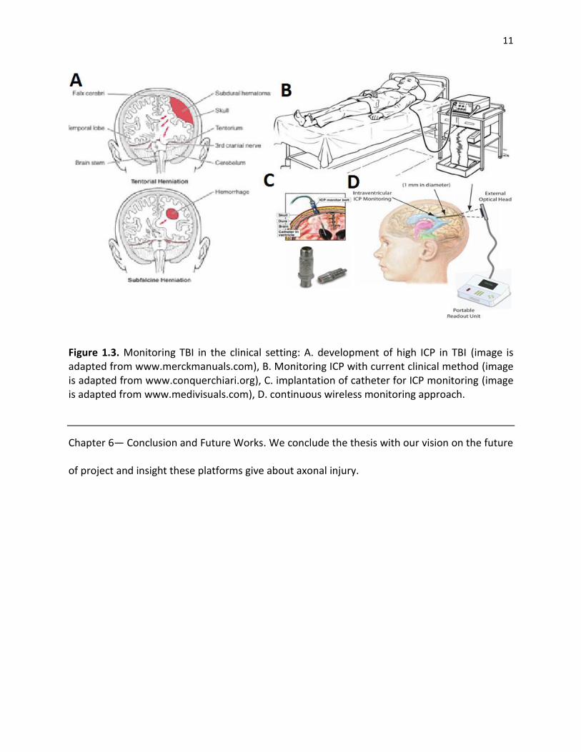
Figure 1.3. Monitoring TBI in the clinical setting: A. development of high ICP in TBI (image is adapted from www.merckmanuals.com), B. Monitoring ICP with current clinical method (image is adapted from www.conquerchiari.org), C. implantation of catheter for ICP monitoring (image is adapted from www.medivisuals.com), D. continuous wireless monitoring approach.
Chapter 6— Conclusion and Future Works. We conclude the thesis with our vision on the future
of project and insight these platforms give about axonal injury.
12
CHAPTER 2
IN-VIVO MECHANICAL STRESS ASSAY: DROSOPHILA LARVA ON MICROFLUIDIC CHIPS
With powerful genetics and a translucent cuticle, the Drosophila larva is an ideal model system
for live imaging studies of neuronal cell biology and function. Here, we present an easy-to-use
approach for high resolution live imaging in Drosophila using microfluidic chips. Two different
designs allow for non-invasive and chemical-free immobilization of 3rd instar larvae over short
(up to 1 hour) and long (up to 10 hours) time periods. We utilized these ‘larva chips’ to
characterize several subcellular responses to axotomy which occur over a range of time scales
in intact, unanaesthetized animals. These include waves of calcium which are induced within
seconds of axotomy, and the intracellular transport of vesicles whose rate and flux within axons
changes dramatically within 3 hours of axotomy. Axonal transport halts throughout the entire
distal stump, but increases in the proximal stump. These responses precede the degeneration
of the distal stump and regenerative sprouting of the proximal stump, which is initiated after a
7 hour period of dormancy and is associated with a dramatic increase in F-actin dynamics. In
addition to allowing for the study of axonal regeneration in vivo, the larva chips can be utilized
for a wide variety of in vivo imaging applications in Drosophila. We also show the chip can be
used for mechanical stimulation of a neuron in-vivo. We use this capability to investigate the

13
effect of various pattern of mechanical signal on the axonal regeneration. It is exceptionally
important as a model for continuous monitoring of pressure in-vivo.
2.1. Introduction
Axons are vulnerable components of neuronal circuitry, hence it is of great interest to
understand how neurons respond to axonal injury. The ability of an axon to regenerate requires
an environment favorable to axonal growth, as well as a series of intrinsic cellular events that
occur on different time scales after injury [21-23]. Within seconds of injury, intracellular levels
of calcium rapidly rise and then decay, and this change in intracellular calcium appears to be an
important precursor to subsequent regeneration [24-26]. Later responses include a
transcriptional response facilitated by an increase in cAMP [27], the retrograde transport of
signaling molecules [28], and an increased transport of cellular components into the axon [29,
30]. Concomitantly, the distal stump, which has been disconnected from the cell body,
undergoes Wallerian degeneration [31] clearing the way for regenerating axon. Importantly,
axonal regeneration also requires the formation of a functional growth cone from the injured
proximal stump. A characteristic feature of the growth cone is its highly dynamic and
coordinated structure of filamentous actin, which allows it to change shape in response to cues
in the environment.
Recently the development of various laser ablation techniques [32] in combination with
microfluidic technology [33] has enabled the in vivo monitoring of regenerative responses to
axonal injury in the nematode C. elegans [34-38]. However, C. elegans neurons display some
behaviors not observed in vertebrate neurons, including re-fusion of the broken axonal
fragments [33, 39, and 40].

14
Here we present a method for monitoring regenerative responses to injury in Drosophila
melanogaster. Like C. elegans, Drosophila larva has a translucent cuticle and a simple
neuroanatomy that is amenable to in vivo imaging [25, 41]. Moreover, axons in the Drosophila
peripheral nervous system are enheathed in glia [42, 43] and undergo Wallerian degeneration
similarly to vertebrate axons [44-46]. Drosophila axons are also capable of undergoing new
axonal growth after injury, and genetic studies indicate that conserved signaling molecules are
required for this process [44, 47].
Despite the great potential, several technical issues need to be addressed in order to
perform in vivo imaging in Drosophila. For high resolution imaging of rapid events such as
calcium waves and axonal transport, the animal needs to be exceptionally stationary during
immobilization. On the other hand, time lapse imaging of long term events such as new axonal
growth requires a gentle immobilization technique which will not interfere with the physiology
of the animal. Conventional immobilization approaches involve dissection [48, 49] or the use of
chloroform to anesthetize the larva [50]. Isofluorane is also used as an anesthetic for long-term,
time-lapse imaging [41, 51]. While the use of anesthetics has many advantages, anesthetics are
known to inhibit neural activity and alter neural physiology [52, 53]. Because the larva can
survive only short doses of the chemical, time-lapse imaging must be restricted to time
intervals of 2 hours in order to allow recovery between doses of the anesthetic [41, 52, 53]. In
addition, human safety concerns must also be taken into account when working with
conventional anesthetics. In order to image cellular events over broader timescales and with
higher throughput, a chemical-free immobilization method is needed.
15
Here, we report a microfluidic-based immobilization methodology for time-lapse
imaging in Drosophila larvae. Our approach employs mechanical forces and/or supply of carbon
dioxide gas (CO2) in order to temporally immobilize single 3rd instar larva. It minimizes the stress
on the larva body (recovery takes place in less than 30 seconds) and allows repetitive in vivo
imaging to be performed over extended periods of time. The proposed microfluidic ‘larva chips’
can be efficiently utilized for imaging various cellular events which occur on different time
scales, ranging from milliseconds up to several hours. While in this work we focus upon cellular
responses to targeted injury of neurons, the microfluidic chips can be broadly used for in vivo
imaging of many different processes in Drosophila larvae.
2.2. In-vivo Imaging of Cellular Responses to Neural Injury
Chip microfabrication. Master molds were microfabricated by spinning and patterning SU-8-
2050 photoresist on silicon wafers. To generate the SI-chip, a 10:1 polydimethylisiloxane
-thick SU-8 mold for 4 hours at 650C. For the
LI-chip, a similar procedure was used to generate two SU-8 molds. The first mold was 170-µm
thick, the second one was 100-µm thick. To fabricate the first PDMS layer of the LI-chip, a 1:15
PDMS mixture was spin cast at 415 rpm and cured over the first SU-8 mold, resulting in a 180-
µm thick PDMS layer. A second PDMS slab that contained the CO2 microchamber was
microfabricated by casting and curing a 10:1 PDMS mixture over the 100-µm thick SU-8 mold
and plasma bonded into the first PDMS layer. Fluidics inlets/outlets outlets were punched into
the PDMS slabs using a sharpened, 19-gauge stainless steel needle.
16
Larva loading. Single early stage 3rd instar larva (~4 mm in length) was immersed in halocarbon
oil 700 (cat. # H8898 Sigma Aldrich Inc.), placed on a glass coverslip, and then manually aligned
and covered with the PDMS microfluidic chip. A tight seal between the PDMS chip and the
coverslip was created by applying weak vacuum (600 mTorr) to the outlet of the microfluidic
network. Vacuum was generated: (i) manually, using a 20 cc syringe in the SI-chip, and (ii) using
a mechanical pump in the LI-chip. CO2 was supplied at the top PDMS layer of the LI-chip at 5 psi.
Imaging. All in vivo imaging recordings were conducted using a spinning disk confocal system
(Perkin Elmer), consisting of a Yokagawa Nipkow CSU10 scanner, and a Hamamatsu C9100-50
EMCCD camera, mounted on a Zeiss Axio Observer with 63x (1.5 NA) oil objective. Volocity
software (Perkin Elmer) was used for all image acquistion and analysis.
Injury assays. Laser injuries were performed using a nanosecond 435 nm pulsed UV dye laser
(Photonic instruments Inc.), as described previously [56]. Nerve crush injuries were performed
by pinching the dorsal part of the animal containing segmental nerves with Dumostar number 5
forceps, as described previously [44].
Calcium imaging. We expressed UAS-GCaMP2.0 [55] with ppk-Gal4 in class IV sensory neurons
[66]. Videos were captured at ~3 frames per second (300 msec exposure time). The cell body
average fluorescence signal was then extracted from each frame and background-corrected
using Volocity software (Perkin Elmer).
Axonal Transport. RRa(eve)Gal4 was used to drive expression of UAS-ANF-GFP specifically in
aCC and RP2 motoneurons [48, 67]. Segmental nerves were imaged continuously at ~5
frames/sec (exposure time was set to 200 milliseconds). To generate kymographs, the

17
collection of single frames spanning one minute of imaging time were processed using the
‘Multiple Kymograph’ plug-in for ImageJ [68]. For analysis, we used a MATLAB program to
automate particle detection and tracking from kymographs. The program uses fast
reconstruction techniques and line tracking methods, along with manual correction, to
delineate individual particle traces. First, the program search for particles in the kymograph
image using regularized Hough transform [69] and tracks each particle using B-Snake method
[70]. The program then removes the trace of detected particles from the kymograph image and
repeats the paricle tracking step until it finds no more particles. Subsequently, the trace of
particles are verified and corrected manually. From each trace, many independent properties
including segment velocities and particle density could be measured. The result then is used to
track and calculate the speed, the number of change in the direction and the density of
particles for each direction (anterograde and retrograde). The data then is analyzed to find
significant difference between different experimental conditions.
Analysis of Axonal Regeneration. Changes in the proximal stump structure were quantified from
time-lapse confocal images collected at a sampling rate of one z-stack of images per min (only
the best-focused images were processed). First, movement artifacts between frames were
reduced using a fast block matching algorithm [71]. For each frame, the area of the proximal
stump was generated using a B-Snake method [70]. The non-overlapping area between two
subsequent frames, representing the area change of the proximal stump, was then calculated.
Finally, the area change was normalized with respect to the area of the proximal stump in each
frame.
18
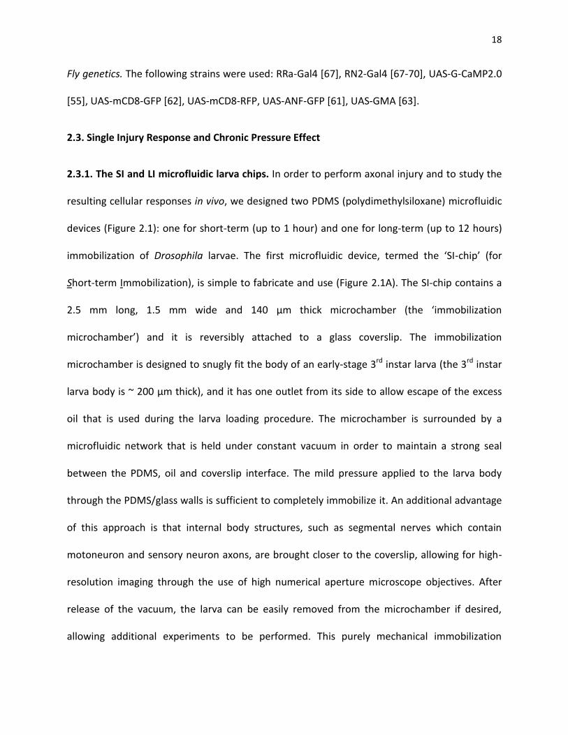
Fly genetics. The following strains were used: RRa-Gal4 [67], RN2-Gal4 [67-70], UAS-G-CaMP2.0
[55], UAS-mCD8-GFP [62], UAS-mCD8-RFP, UAS-ANF-GFP [61], UAS-GMA [63].
2.3. Single Injury Response and Chronic Pressure Effect
2.3.1. The SI and LI microfluidic larva chips. In order to perform axonal injury and to study the
resulting cellular responses in vivo, we designed two PDMS (polydimethylsiloxane) microfluidic
devices (Figure 2.1): one for short-term (up to 1 hour) and one for long-term (up to 12 hours)
immobilization of Drosophila larvae. The first microfluidic device, termed the ‘SI-chip’ (for
Short-term Immobilization), is simple to fabricate and use (Figure 2.1A). The SI-chip contains a
2.5 mm long, 1.5 mm wide and 140 µm thick microchamber (the ‘immobilization
microchamber’) and it is reversibly attached to a glass coverslip. The immobilization
microchamber is designed to snugly fit the body of an early-stage 3rd instar larva (the 3rd instar
larva body is ~ 200 µm thick), and it has one outlet from its side to allow escape of the excess
oil that is used during the larva loading procedure. The microchamber is surrounded by a
microfluidic network that is held under constant vacuum in order to maintain a strong seal
between the PDMS, oil and coverslip interface. The mild pressure applied to the larva body
through the PDMS/glass walls is sufficient to completely immobilize it. An additional advantage
of this approach is that internal body structures, such as segmental nerves which contain
motoneuron and sensory neuron axons, are brought closer to the coverslip, allowing for high-
resolution imaging through the use of high numerical aperture microscope objectives. After
release of the vacuum, the larva can be easily removed from the microchamber if desired,
allowing additional experiments to be performed. This purely mechanical immobilization

19
approach can keep >90% of larvae alive for continuous immobilization periods of up to 1 hour
(Figure 2.2A).

20
Figure 2.1. The SI and LI microfluidic chips for immobilizing Drosophila larva. (A) the SI-chip is a single-layer PDMS microfluidic device that utilizes a shallow (140 µm thick) immobilization microchamber to squeeze larvae in the vertical direction. Scale bar, 1 mm. (B) the two-layer LI-chip. The first PDMS layer (labeled with blue color) has the larva immobilization microchamber and is connected to two microfluidic channels to supply food to the larva head (typically delivered every 30 min). A second PDMS layer (labeled with red color) is vertically integrated into the first PDMS layer to deliver CO2 through a 10-µm thick PDMS membrane. In both the SI and LI chips, a microfluidic network surrounding the immobilization chamber is used to create a tight seal between the PDMS and the glass coverslip. Scale bar, 1 mm. (C) (I) Bright-field image of a 3rd instar larva immobilized in the LI-chip. Scale bar, 1 mm. (II) Fluorescent images of the larva body (highlighted in the red square in C(I)) before (top image) and after (bottom image) immobilization. After application of CO2 at 5 psi, the larva is immobilized and the GFP-labeled ventral nerve cord is brought into focus (bottom image). Scale bar, 20µm.
Figure 2.2. Survival rates and body movement of on-chip immobilized larvae. (A) Survival rate of continuously immobilized larvae using the SI-chip. Five different immobilization microchambers thicknesses were tested. We considered a thickness of 140 µm (red curve) to be optimal, as thicknesses higher than 140 µm resulted in poor immobilization. (B) Survival rates on the LI-chip using periodic immobilization (30 s of immobilization every 5 min). We considered a thickness of 170 µm (red curve) to be optimal as more than 85% of larvae survived the immobilization
21
procedure after 10 hours. (C) Average larva body movement using the LI-chip for different thicknesses of the immobilization microchamber (30 s of immobilization every 5 min). In all plots, error bars represent standard error of the mean obtained from 10 larvae.
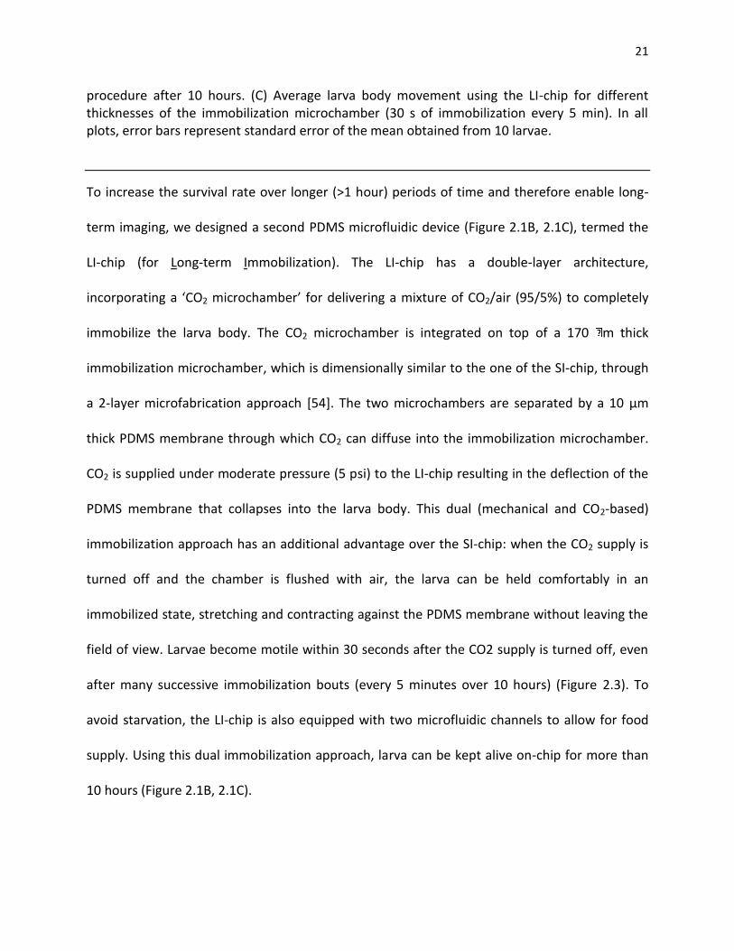
To increase the survival rate over longer (>1 hour) periods of time and therefore enable long-
term imaging, we designed a second PDMS microfluidic device (Figure 2.1B, 2.1C), termed the
LI-chip (for Long-term Immobilization). The LI-chip has a double-layer architecture,
incorporating a ‘CO2 microchamber’ for delivering a mixture of CO2/air (95/5%) to completely
immobilize the larva body. The CO2 microchamber is integrated on top of a 170 m thick
immobilization microchamber, which is dimensionally similar to the one of the SI-chip, through
a 2-layer microfabrication approach [54]. The two microchambers are separated by a 10 µm
thick PDMS membrane through which CO2 can diffuse into the immobilization microchamber.
CO2 is supplied under moderate pressure (5 psi) to the LI-chip resulting in the deflection of the
PDMS membrane that collapses into the larva body. This dual (mechanical and CO2-based)
immobilization approach has an additional advantage over the SI-chip: when the CO2 supply is
turned off and the chamber is flushed with air, the larva can be held comfortably in an
immobilized state, stretching and contracting against the PDMS membrane without leaving the
field of view. Larvae become motile within 30 seconds after the CO2 supply is turned off, even
after many successive immobilization bouts (every 5 minutes over 10 hours) (Figure 2.3). To
avoid starvation, the LI-chip is also equipped with two microfluidic channels to allow for food
supply. Using this dual immobilization approach, larva can be kept alive on-chip for more than
10 hours (Figure 2.1B, 2.1C).

22
The dual immobilization capability of LI-chip can also be used for mechanical stimulation
of larva. The larva is immobilized using low pressure (10 psi) CO2 gas diffusion. The pressure
higher than 10psi is used to stimulate the neuron mechanically. The higher CO2 pressure does
not affect the immobilization and imaging of larva.
Figure 2.3. Recovery after immobilization. Animals are immobilized for 30 seconds under different conditions. The body movement, first the animal is imaged (5 frame/sec). The movement between frames was calculated using a fast block matching algorithm. The body movement is recorded over a time course from 15 seconds before immobilization to 50 seconds after immobilization. To measure The red line represents the average body movement of 10 samples. The grey lines represents average movement recorded from 10 larva. The dashed line indicates the time of immobilization. (A) After immobilization with pressure alone (5 psi air pressure, 30 seconds), larvae regain full mobility within 10 seconds. (B) After immobilization with 95/5% CO2/air, the larvae regain full motility within 30 seconds after releasing the pressure. (C) Larvae were immobilized every 5 minutes for 10 hours in the LI-chip, and then

23
assayed for recovery after 30 seconds of immobilization with 95/5% CO2/air. The larvae still recover within 30 seconds, similarly to (B).
2.3.2. On-chip calcium imaging within milliseconds of injury. The SI-chip enabled us to perform
laser axotomy and measurement of rapid changes in the intracellular calcium after injury. To
detect the change in the intracellular calcium level, we used the genetically encoded calcium
sensor G-CaMP 2.0 [55] which was expressed in Class IV sensory neurons via the Gal4/UAS
system (Figure 2.4 describes the neurons and drivers utilized). After immobilizing single larva in
the SI-chip, a pulsed UV dye laser was used to transect a single dendrite [56]. Injury induced an
instant and dramatic increase at the G-CaMP fluorescence level (F) at the injury site, which
rapidly spread along both the proximal and distal compartments of the dendrite (Figure 2.5A).
Within 2 seconds after injury, a ~200% increase in fluorescence (ΔF/F0 ≈ 2, where F0 is the
baseline fluorescence level before injury) was detected in the cell body, which returned to
baseline levels within 15 seconds (Figure 2.5B). For comparison, mCD8-GFP expressed in the
same neurons, did not yield a significant change in intensity after laser axotomy (Figure 2.5B,
2.5C). The kinetics of the observed Ca2+ responses resemble Ca2+ transients to axonal injury in
other model organisms [25, 26, 57, 58]. The SI-chip can therefore be used to perform in vivo
laser microsurgery on-chip as well as to quantify the resulting responses.
2.3.3. Monitoring changes in axonal transport after injury. Microtubule-based motors,
kinesins and dynein, are known to carry vesicles and organelles at rates of 0.1-5 µm/sec in
axons [59, 60]. Documentation of this motility requires rapid imaging with high magnification,
high numerical aperture objectives, and precise immobilization of the larva. Dense core
synaptic vesicles, labeled by expressing ANF-GFP [61] specifically in aCC and RP2 motorneurons
24
using the Gal4/UAS system, were imaged in intact larvae using the SI-chip and in dissected
‘flay-open’ larvae as previously described [44]. Image analysis revealed a slight difference in
segment velocity between the two methods (data are not shown); however the overall
anterogradely and retrogradely particle density (particles / 100 µm of axon length) did not
change significantly (Figure 2.6). We conclude that the SI-chip is an effective method for
imaging and measuring properties of axonal transport, equivalent to the ‘flayed open’
approach.
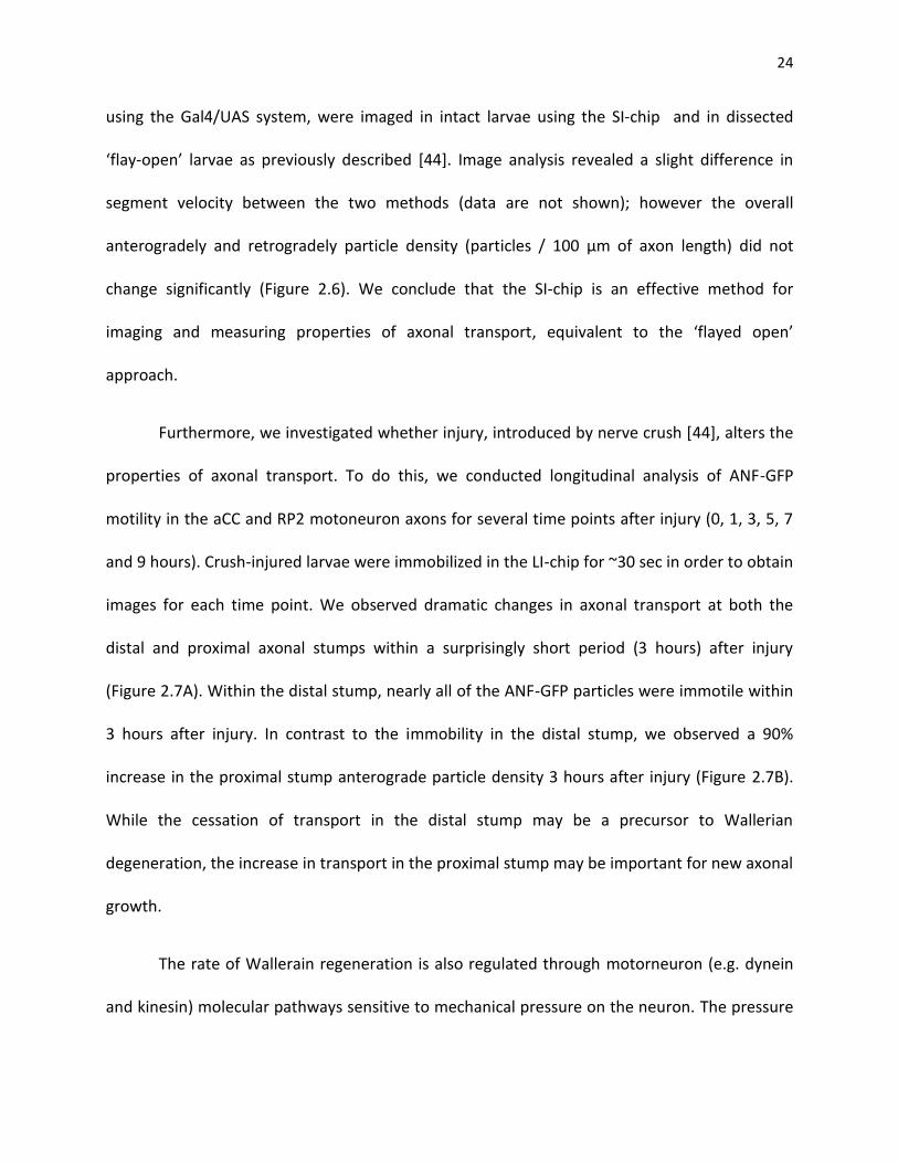
Furthermore, we investigated whether injury, introduced by nerve crush [44], alters the
properties of axonal transport. To do this, we conducted longitudinal analysis of ANF-GFP
motility in the aCC and RP2 motoneuron axons for several time points after injury (0, 1, 3, 5, 7
and 9 hours). Crush-injured larvae were immobilized in the LI-chip for ~30 sec in order to obtain
images for each time point. We observed dramatic changes in axonal transport at both the
distal and proximal axonal stumps within a surprisingly short period (3 hours) after injury
(Figure 2.7A). Within the distal stump, nearly all of the ANF-GFP particles were immotile within
3 hours after injury. In contrast to the immobility in the distal stump, we observed a 90%
increase in the proximal stump anterograde particle density 3 hours after injury (Figure 2.7B).
While the cessation of transport in the distal stump may be a precursor to Wallerian
degeneration, the increase in transport in the proximal stump may be important for new axonal
growth.
The rate of Wallerain regeneration is also regulated through motorneuron (e.g. dynein
and kinesin) molecular pathways sensitive to mechanical pressure on the neuron. The pressure

25
primary changes the rate of neuron membrane diffusion. The rate of down regulation of a
pathway associated with the pressure could be measure by imaging axonal transports including
the density of stationary particle and speed of moving particles in the axon segment proximal to
the site of injury.
Figure 2.4. Diagram of neurons and Gal4 drivers. (A) Class IV sensory neurons (blue), labeled by ppk-Gal4, were used to study the Ca2+ responses to laser ablation of a dendrite (in Figure 2) because both their cell bodies and dendrites lie close the cuticle, allowing for excellent reproducible injury by the pulsed dye laser, and excellent visualization of cellular responses close to injury site. B) The eve(RRa)Gal4 driver expresses specifically in aCC and RP2 motneurons (green). These were used for the study of axonal transport after nerve crush injury

26
(in Figure 3) because the regenerative response to injury has been previously characterized in these neurons. (C) The RN2-Gal4 driver line, which labels enteric motoneurons in larvae (red), was used for the time lapse study of regeneration. This driver line is very strong, allowing for both UAS-GMA and UAS-mCD8-RFP to be expressed at high levels. While these neurons display similar reactions to both laser axotomy and nerve crush, we focused upon laser axotomy for Figure 4 because this injury is small enough to fit within one field of view.
Figure 2.5. Calcium dynamics after laser axotomy. (A) Time-lapse images from immobilized larvae depict intracellular calcium dynamics during laser microsurgery. Sensory neurons expressing G-CaMP and GFP were ablated with a pulsed UV laser (see also supplementary movies 1 and 2). (B) Average normalized fluorescent intensity (ΔF/F0) from G-CaMP and GFP expressing neural cell bodies (sample size, n = 12) before and after injury (injury is performed at 0 sec). A peak value in the intensity of G-CaMP is observed 2 seconds after injury. Calcium transients from individual larvae are depicted in light grey color. (C) Quantification of the maximum fluorescent intensity change (maximum ΔF/F0). The fluorescent intensity from GFP expressing neurons did not change significantly (p-value < 0.01, n =12).

27
The high pressure also can affect the initial stage of injury response. High pressure can reduce
the rate of extracellular calcium diffusion into the cell, reducing the calcium response to injury
in the few first second of injury and resulting in weaker injury response in the long-term.
Figure 2.6. Changes in axonal transport after nerve-crush injury. (A) Kymographs of ANF-GFP labeled vesicles in an uninjured axon, and 3 hours after injury in the distal stump and proximal stump. (B) Particle density (anterograde, retrograde, and stationary) was quantified per 100 µm of axon length. In the proximal stump 3 hours after injury, there was a 90% increase in anterograde particle density (p-value = 0.03, n = 16), but no significant change in retrograde particle density (p-value < 0.01, n = 16). In contrast, transport was almost completely halted in the distal stump (p value < 0.01, n = 8). Error bars represent standard error of the mean.
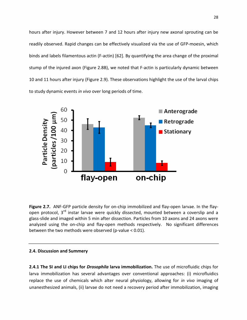
2.3.4. Long-term, time-lapse imaging of axonal sprouting after injury. The ideal method for
studying and quantifying regenerative axonal growth is to conduct longitudinal time-lapse
imaging of single axons after injury. We tracked the proximal and distal stumps of an injured
axon by collecting high-resolution confocal images throughout a 5-hour (7-12 hours) time
course (Figure 2.8). Larvae remained immobilized only during image acquisition (30 sec for
every 1 minute). We observed that the proximal stump is relatively dormant for the first seven
28
hours after injury. However between 7 and 12 hours after injury new axonal sprouting can be
readily observed. Rapid changes can be effectively visualized via the use of GFP-moesin, which
binds and labels filamentous actin (F-actin) [62]. By quantifying the area change of the proximal
stump of the injured axon (Figure 2.8B), we noted that F-actin is particularly dynamic between
10 and 11 hours after injury (Figure 2.9). These observations highlight the use of the larval chips
to study dynamic events in vivo over long periods of time.
Figure 2.7. ANF-GFP particle density for on-chip immobilized and flay-open larvae. In the flay-open protocol, 3rd instar larvae were quickly dissected, mounted between a coverslip and a glass-slide and imaged within 5 min after dissection. Particles from 10 axons and 24 axons were analyzed using the on-chip and flay-open methods respectively. No significant differences between the two methods were observed (p-value < 0.01).
2.4. Discussion and Summery
2.4.1 The SI and LI chips for Drosophila larva immobilization. The use of microfluidic chips for
larva immobilization has several advantages over conventional approaches: (i) microfluidics
replace the use of chemicals which alter neural physiology, allowing for in vivo imaging of
unanesthesized animals, (ii) larvae do not need a recovery period after immobilization, imaging
29
over a broad range of time scales is therefore possible, (iii) the immobilization conditions are
reproducible and well-controllable (iv) the microfluidic chips are simple to fabricate and their
design can be easily adapted to immobilize larvae of different developmental stages or many
larvae at once. While we described in this report the use of microfluidics for studying responses
to neural injury, we envision that the proposed chips can be broadly used to study many
different cellular events in vivo. Examples include the formation of new synaptic contacts at
neuromuscular junctions, the motility of cytosolic components in neurons, muscles, or glia, and
calcium signaling within individual cells as an indicator of neural activity.
Figure 2.8. Axonal regeneration after laser injury. (A) In vivo time-lapse images of the regeneration process 7 hours to 12 hours after laser axotomy. The proximal site (PS) of injury, the site of injury (SOI), and the distal site (DS) of injury are highlighted right after injury (0:00

30
frame). The red color represents RFP expression that is localized in the membrane of the axon. The green color represents F-actin expression. Scale bar, 10 µm. (b) Normalized area change of the proximal stump over time. Significant movement in the proximal stump is observed ~10.5 hours after injury.
Figure 2.9. On-chip axon regeneration after laser axotomy. (a) In vivo time-lapse images of the proximal site (PS) of injury, the site of injury (SOI), and the distal site (DS) of injury, 10 hours after laser axotomy. The red color represents red fluorescent protein (RFP) expressed in the membrane of the axon. The green color represents F-actin. Scale bar, 10 µm. (b) Normalized area change of the proximal stump between 10 and 11 hours after injury.
2.4.2. The SI chip allows for in vivo imaging of neural activity. The in vivo study of neural
activity (e.g. through Ca2+ imaging) requires the development of whole-animal immobilizing
methods that do not affect neural physiology. Our non-invasive, purely mechanical-based
approach for immobilizing live larvae creates an ideal environment for measuring intracellular
31
Ca2+ dynamics in vivo. We observed that laser microsurgery of a single neurite induced a wave
of Ca2+ similar to injury in other model organisms [25, 26, 57, and 58]. This method, coupled
with well-established genetic approaches in Drosophila, will allow for a better understanding of
the role of Ca2+ dynamics in axonal regeneration and degeneration processes after injury.
2.4.3. The larva chips allow monitoring of rapid changes in axonal transport. The SI and LI
microfluidic chips was particularly useful for studying changes in axonal transport after injury,
which we were unable to study over long periods of time in dissected animals. We observed
rapid and asymmetric changes in axonal transport in proximal and distal sides of the injury, with
an increase in anterograde transport in the proximal stump, and a cessation of all transport in
the distal stump. This dichotomy on either side of the injury site correlates with the opposite
outcomes: the proximal stump of the aCC and RP2 neurons initiate new axonal growth and
branching, while the distal stumps undergo Wallerian degeneration [54].
The cessation of transport throughout the entire distal stump within 3 hours of injury
parallels previous observations in mice that mitochondrial transport in the distal process halts
within a similar time frame [63]. Interestingly, fragmentation of the axonal membrane and
microtubules for these neurons does not begin until about 6 hours after injury, so the cessation
of transport and may represent an early stage in the process of Wallerian degeneration.
Because transport halts throughout the entire distal process, it may involve a rapidly diffusing
cue, such as calcium, from the injury site. In contrast to the distal stump, the number of
anterogradely moving particles increases in the proximal stump within 3 hours of injury. This

32
increase in axonal transport parallels observations in vertebrate peripheral axons and may play
an important role in promoting new axonal growth [29, 30].
2.4.4. Studying regenerative responses on-chip. Microfluidics techniques have previously
enabled the study of axonal regeneration after injury in C. elegans [33]. However C. elegans
neurons display some behaviours after injury that are seldom observed in vertebrate neurons,
For instance, C. elegans axons can regrow along the distal stump, and can sometimes re-fuse
with the distal stump, which often fails to undergo Wallerian degeneration [35, 36, and 39]. In
contrast, Drosophila axons resemble vertebrate axons in that the proximal stump undergoes
extensive sprouting but never makes contact with the distal stump, and may indeed be repelled
by the distal stump [64, 65].
Using the LI-chip, we observed that the proximal stump begins to undergo profound
morphological changes after a period of dormancy. The minute-to-minute changes in F-actin
structure suggest the existence of a dynamic network of actin, which would be a fundamental
component of a functional growth cone. It is intriguing that the dynamics are not observed
immediately after injury, but require at least 7 hours after injury to be initiated. Previously
characterized transcriptional responses to injury require a similar time course in Drosophila
neurons [44], so this time of dormancy may reflect the need for new gene expression or
transport of new material in order to form a new growth cone. In future studies, it will be
interesting to determine the cellular requirements for initiation of those dynamics, using
Drosophila larva as a genetically tractable model system.
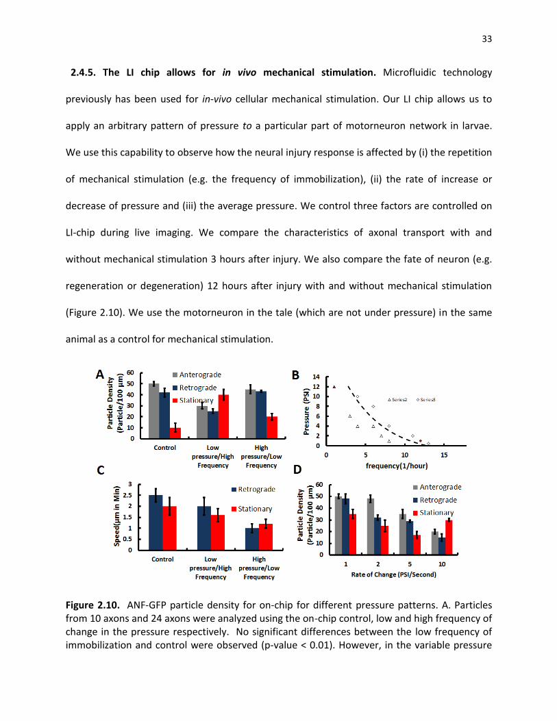
33
2.4.5. The LI chip allows for in vivo mechanical stimulation. Microfluidic technology
previously has been used for in-vivo cellular mechanical stimulation. Our LI chip allows us to
apply an arbitrary pattern of pressure to a particular part of motorneuron network in larvae.
We use this capability to observe how the neural injury response is affected by (i) the repetition
of mechanical stimulation (e.g. the frequency of immobilization), (ii) the rate of increase or
decrease of pressure and (iii) the average pressure. We control three factors are controlled on
LI-chip during live imaging. We compare the characteristics of axonal transport with and
without mechanical stimulation 3 hours after injury. We also compare the fate of neuron (e.g.
regeneration or degeneration) 12 hours after injury with and without mechanical stimulation
(Figure 2.10). We use the motorneuron in the tale (which are not under pressure) in the same
animal as a control for mechanical stimulation.
Figure 2.10. ANF-GFP particle density for on-chip for different pressure patterns. A. Particles from 10 axons and 24 axons were analyzed using the on-chip control, low and high frequency of change in the pressure respectively. No significant differences between the low frequency of immobilization and control were observed (p-value < 0.01). However, in the variable pressure
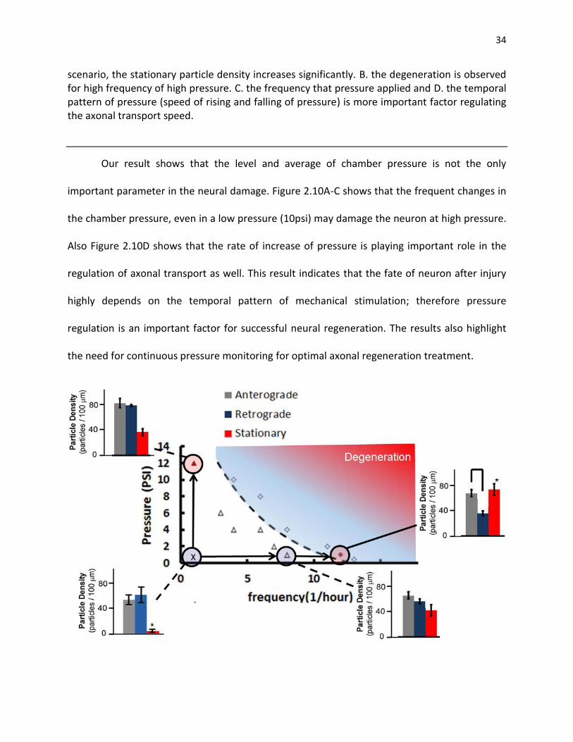
34
scenario, the stationary particle density increases significantly. B. the degeneration is observed for high frequency of high pressure. C. the frequency that pressure applied and D. the temporal pattern of pressure (speed of rising and falling of pressure) is more important factor regulating the axonal transport speed.
Our result shows that the level and average of chamber pressure is not the only
important parameter in the neural damage. Figure 2.10A-C shows that the frequent changes in
the chamber pressure, even in a low pressure (10psi) may damage the neuron at high pressure.
Also Figure 2.10D shows that the rate of increase of pressure is playing important role in the
regulation of axonal transport as well. This result indicates that the fate of neuron after injury
highly depends on the temporal pattern of mechanical stimulation; therefore pressure
regulation is an important factor for successful neural regeneration. The results also highlight
the need for continuous pressure monitoring for optimal axonal regeneration treatment.

35
Figure 2.11. Effect of frequency and pressure level on the survival of neurons. A. Particles from 10 axons and 24 axons were analyzed using the on-chip control, low and high frequency of change in the pressure respectively.The survival rate is analyzied in different pressure levels

36
CHAPTER 3
OPTO-MECHANICAL MICROSENSOR FOR INTRACRANIAL PRESSURE MONITORING
Most brain injuries are caused by some form of trauma such as car accident, blast or a fall. In
most cases the secondary damage caused by elevated cranial pressure is even more harmful
than initial impact. Managing the damage to brain tissue after the trauma requires continuous
long-term monitoring. In this chapter, a new family of implantable, wireless and power-free
optical microsensors is presented that can potentially be used to accurately monitor
intracranial pressure (ICP) over long periods of time. These microsensors vertically integrate a
glass mini-lens with a two-wavelength quantum dot micropillar that is photolithographically
patterned on an ICP-exposed silicon nitride membrane. The operation principle is based on a
novel opto-mechanical transduction scheme that converts ICP changes into changes in the
intensity ratio of the two-wavelength, near infrared fluorescent light emitted from the quantum
dots. These microsensors are microfabricated using silicon bulk micromachining and they
operate at an ICP clinically relevant pressure dynamic range (0-40mmHg). They have a
maximum error of less than 15 % throughout their dynamic range and they are extremely
photostable. We believe that the proposed microsensors will open up a new direction not only
in ICP monitoring but in other pressure-related biomedical applications.
37
3.1. Introduction
Intracranial pressure (ICP) monitoring is widely used to evaluate therapeutic interventions in
patients with severe traumatic brain injuries (TBIs), hydrocephalus and other ICP-elevated
disorders [71-73]. ICP monitoring has shown to reduce the number of deaths by 20%, to
minimize secondary brain damage, and to significantly decrease recovery time after surgery
[74-76].
Current ICP monitoring practices often employ a catheter that records the pressure of
the cerebrospinal fluid (known as ‘intraventricular ICP monitoring’). The catheter is surgically
inserted through a burr hole into the ventricles of the brain, which contains the cerebrospinal
fluid. Alternatively, a non-fluid conducting device can be placed into the epidural,
intraparenchymal, or subdural-subarachnoid compartments of the brain, although such ICP
measurement is not considered to be as accurate when compared to intraventricular ICP
monitoring [77, 78]. The ICP pressure level is measured by a piezoresistive [79, 80], a capacitive
[81, 82] or an optical pressure transducer [83] that is attached to the tip of the catheter. In all
cases, the catheter is connected via a cable to the bedside ICP-monitoring unit that reports the
corresponding ICP value. These catheter-based systems have been successful so far in
accurately monitoring ICP, but they are not appropriate for long term ICP monitoring as: (i) the
patient is continuously connected to the non-portable ICP-monitoring unit, and (ii) the long
term placement of the catheter significantly increases the risk of infection / meningitis through
the skull incision (the catheter needs to be removed 3-5 days after placement to minimize the
risk of infection) [77]. Other complications include intracranial hemorrhages and brain injury
during catheter placement due to the large size of the catheter [84, 85] and device malfunction

38
[86]. It is also beneficial in some cases to conduct MRI scans in ICP-monitored patients, a
feature that is not available by current technology.
Recent advances in microengineering have spawned an increasing interest in developing
a new class of fully implantable, MEMS (MicroElectroMechanical Systems)-based ICP
monitoring systems that can potentially provide long term ICP monitoring [87, 88]. These
systems utilize a battery operated capacitive pressure sensor and integrate a CMOS circuit for
wirelessly transmitting the ICP measurements to a portable readout unit. RF telemetry has also
been proposed for batteryless, long-term pressure sensing [89, 90]. Such an approach
generates weak RF signals and thus requires an antenna/readout unit to be placed in close
proximity with the implanted sensor. Moreover, the presence of electronic components makes
these transducers bulky (they typically have a footprint of 0.5-1 cm2) and MRI incompatible
[74].
The requirements for small sensor size in order to eliminate brain damage during
implantation and efficient wireless data/power transmission have limited the use of these
MEMS devices in cardiovascular applications [89] and epidural ICP monitoring [91] (epidural
ICP monitoring is typically avoided as it results in inaccurate ICP measurements [92]). Most
importantly, it is not clear how these systems can evolve to meet the strict FDA regulations for
low power transmission and MRI compatibility in the brain and what the long term side-effects
of placing a wireless implant inside the brain are (e.g. tumor-genesis due to electromagnetic
radiation [93]).
Here, we propose a novel ICP monitoring technology, termed ‘Near infrared
Fluorescent-based Optomechanical (NiFO) pressure sensing technology (Figure 3.1). NiFO

39
technology is based on a fully implantable, optical, powerless sensor (the NiFO sensor) that
converts ICP into a two-wavelength optical signal in the near infrared (NI) spectrum. The NiFO
sensor has unique properties as it: (i) eliminates the risk of infection and thus permits life-long
ICP monitoring, (ii) allows patient mobility after the surgery, (iii) is MRI compatible, and (iv)
induces minimum damage during implantation (the NiFO sensor has a footprint of less than 6.5
mm2). We envision that the proposed NiFO sensing technology will not only help in efficiently
managing ICP-elevated medical conditions, but it will inaugurate a new era in the development
of implantable, electronic and power-free, miniaturized devices that can be used in a variety of
biomedical pressure monitoring applications.
Figure 3.1. (A) The NiFO technology. The external optical readout unit is used to collect spectroscopic data from the implanted NiFO sensor in the near infrared (NI). (B) Cross sectional view of the NiFO sensor. (C) The working principle of the ICP sensor. (D) The microfabricated device sitting on a penny. Chip III has been removed to illustrate the presence of the mini-lens. A 1.6 mm x 1.6 mm silicon nitride membrane with a patterned QD micropillar is shown in the inset. Scale bar, 1 mm.
40
3.2. NiFO Sensing Technology
3.2.1. Sensor Architecture
The proposed ICP monitoring technology consists of the implantable NiFO sensor and an
external (non-implantable), portable readout unit (Figure 3.1A). That readout unit integrates a
NI laser source and a spectrometer that are used to excite, collect and analyze the emitted
fluorescent light from the NiFO sensor. Operating the NiFO sensor in the NI regime is critical for
minimizing light absorption by the skin and the brain tissue [94].
The implantable NiFO sensor consists of three silicon chips stacked together (Figure
3.1B): (i) chip I integrates a flexible membrane with a 4-layer quantum dot (QD) structure (the
‘QD micropillar’) that emits a two-color NI fluorescent light, (ii) chip II contains a plano-convex,
non-microfabricated lens (we use the term ‘mini-lens’) and, (iii) chip III contains an aperture
that permits optical access to chip I while protecting the mini-lens. The plano-convex mini-lens
of chip II focuses incoming NI light into the 4-layer QD micropillar. The 2nd and 4th layers of the
QD micropillar (Figure 3.1B) are made out of QDs [95] of a specific NI wavelength (705 nm and
800 nm respectively) while the 1st and 3rd layers are transparent and function as optical spacers.
The back side of the thin membrane is exposed to the ICP while the front side is sealed in
atmosphere pressure using chip II. When the membrane deflects due to a change in ICP, the QD
micropillar moves with respect to the focal point of the mini-lens (the mini-lens is contained in
an airtight chamber) (Figure 3.1C). Incoming collimated light after passing through the mini-lens
is focused to a finite focal volume that excites both QDs layers. The emitted fluorescent
intensity ratio between the two QD wavelengths (705 nm / 800 nm ratio) depends on the exact
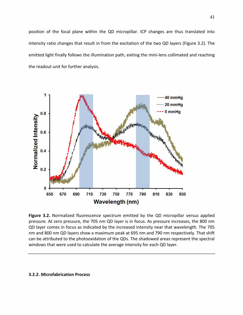
41
position of the focal plane within the QD micropillar. ICP changes are thus translated into
intensity ratio changes that result in from the excitation of the two QD layers (Figure 3.2). The
emitted light finally follows the illumination path, exiting the mini-lens collimated and reaching
the readout unit for further analysis.
Figure 3.2. Normalized fluorescence spectrum emitted by the QD micropillar versus applied pressure. At zero pressure, the 705 nm QD layer is in focus. As pressure increases, the 800 nm QD layer comes in focus as indicated by the increased intensity near that wavelength. The 705 nm and 800 nm QD layers show a maximum peak at 695 nm and 790 nm respectively. That shift can be attributed to the photooxidation of the QDs. The shadowed areas represent the spectral windows that were used to calculate the average intensity for each QD layer.
3.2.2. Microfabrication Process

42
3.2.2.1. Chips I, II and III. We used three double-sided polished silicon wafers (wafers I, II and III
corresponding to chips I, II and III) and standard surface and bulk micromachining techniques to
fabricate the NiFO sensor (Figure 3.3). Wafers I and III had a thickness of 490 m, wafer II had a
thickness of 200 m. We initially LPCVD deposited a 300 nm thick, low-stress silicon nitride film
in all silicon wafers. To fabricate wafer I, we first patterned the QD micropillar on the front side
of the wafer (see the next paragraph for a detailed description of that process). A square
opening was RIE-patterned on the silicon nitride layer on the back side of the wafer. The wafer
was then KOH-etched to obtain the suspended silicon nitride membrane. During that KOH-etch
step, the front side of the wafer containing the QD micropillar was protected using a custom-
made wafer holder. The two silicon nitride membranes of wafers II and III were formed by
following an identical KOH-etch process. Individual 2.5 mm x 2.5 mm chips were finally
obtained by wafer dicing. To complete the fabrication of chip II, a commercially available 1 mm
diameter, plano-convex mini-lens (uncoated with an effective focal length of 0.6 mm, Edmund
Optics Inc., cat. # NT45-588) was manually placed and UV-bonded on top of the silicon nitride
membrane. The UV-bonding step was inspired by the microimprinting process [96]: the planar
surface of the mini-lens was coated with a thin photoresist film by dipping the mini-lens into an
uncured 10 m thick SU-8 2010 layer that had been previously spun on top of a bare silicon
wafer. The mini-lens was then gently placed and optically aligned at the center of the silicon
nitride membrane of chip II. The mini-lens/chip II assembly was finally exposed to ultraviolet
(~355 nm) light for 5 s and heated up in 90oC for 5 min to harden the SU-8 film. That step
resulted in the permanent attachment of the mini-lens to the silicon nitride membrane.

43
Following a similar microimprinting and alignment procedure, chip II was bonded to chip I and
chip I-II assembly was bonded to chip III.
Figure 3.3. The NiFO sensor consists of three chips, manually assembled on top of each other. Each chip has a transparent, 300 nm thick silicon nitride membrane. The key element of the design, the QD micropillar, consists of two QD layers and two SU-8 layers that are photolithographically patterned on top of the ICP-exposed membrane of wafer I.
3.2.2.2. Microfabrication of the QD micropillar. QDs suspended in decane with emission
wavelengths of 705 nm and 800 nm were purchased from Invitrogen Inc. (cat. # Q21761MP and
Q21771MP). The QDs were flocculated from decane by mixing the suspension with a 3:1
methanol:isopropanol solution and centrifuging the mixture at 3000 RPM for 4 minutes. The
supernatant liquid was then discarded and the QDs were resuspended in a 1:1
chloroform:chlorobenzene solution. The volume of solution was adjusted to achieve a 800 pM
concentration of the 705 nm QDs. To achieve similar emission intensity, a higher concentration
44
(1200 pM) was used for the preparation of the 800 nm QD solution. The QD solutions were
then mixed with a tetraphenyl diaminobiphenyl (TPD) solution (100 mg of TPD were dissolved
in 1 ml of chlorobenzene) in 1:1 ratio resulting in a final concentration of 400 pM and 600 pM of
705 nm and 800 nm QDs respectively. The resulting QD/TPD solution has the unique property
of forming an extremely thin and uniform layer of QDs on a flat surface when the solvent (TPD)
evaporates [97].
The QD micropillar consisted of two layers of QDs and two transparent SU-8 layers.
Initially, a 2 m thick SU-8 layer was spun on a silicon nitride coated silicon wafer (wafer I). The
800 nm QD layer was made by spinning the 800 nm QD/TPD solution on the SU-8 coated wafer
at 2000 rpm and allowing for the solvent to evaporate by a two-step heating process (65oC for 3
min and 95 oC for 5 min). SU-8 2015 photoresist was then spun at 1000 rpm and soft baked at
the top of first QD layer to form a 18 m thick layer. The 705 nm QD/TPD solution was then
spun and heated on top of the SU-8 layer following an identical procedure to the one described
above. The entire QD micropillar was more than 90% transparent in the 650 nm - 800 nm range
and showed no detectable fluorescence (data not shown).
3.3. Results and Discussion
3.3.1 Membrane Deflection Versus Pressure.
The membrane deflection-pressure dependence is a critical aspect of the sensor design as it
defines the dynamic range and resolution of the NiFO sensor. To obtain that dependence, we
exposed the backside of the silicon nitride membrane of chip I to a pressure range that
represented physiological (0-20 mmHg) and elevated ICP cases (20-40 mmHg). The topside of

45
the membrane was exposed to atmospheric pressure (for this set of experiments we did not
integrate chips II and III). A distilled water column was used to apply the desired pressure level
while the membrane deflection was measured using an epi-fluorescent microscope. The
microscope was equipped with a piezoelectric z-stage that allowed us to bring the center of the
membrane in sharp focus and accurately extract the membrane displacement at a given
pressure. A 705 nm QD layer, spun on top of the membrane following the procedure described
above, was used to obtain high-contrast fluorescent images of the deflected membrane.
We obtained deflection-ICP curves for square membranes of 5 different dimensions (0.
8 mm x 0.8 mm, 1 mm x 1 mm, 1.2 mm x 1.2 mm, 1.4 mm × 1.4 mm and 1.6 mm × 1.6 mm)
(Figure 3.4). The pressure was manually regulated from 0 mmHg to 40 mmHg by adjusting the
height of the water column and the corresponding membrane deflection was measured for
every 2.5 mmHg. The results depict a non-linear regime at the physiological ICP range (0-20
mmHg) and a linear regime at higher pressures (20-40 mmHg) (the linear correlation coefficient
was 0.99 when pressure was in the 20 - 40 mmHg range). No plastic deformation was observed,
as loading-unloading deflection measurements from the same membrane had a relative
standard error (RSE) of 3.1% throughout the entire ICP range (RSE is the standard error of the
mean expressed in percentage). Deflection measurements from membranes obtained from
different wafers had a RSE of 6.8% which can be attributed mainly to the silicon nitride film
thickness variations (2.3% variation from wafer to wafer and 1.2% variation across a wafer). It is
also worth noticing that none of the membranes failed at the maximum applied pressure of 40
mmHg after repetitive loading conditions, indicating a robust operation.
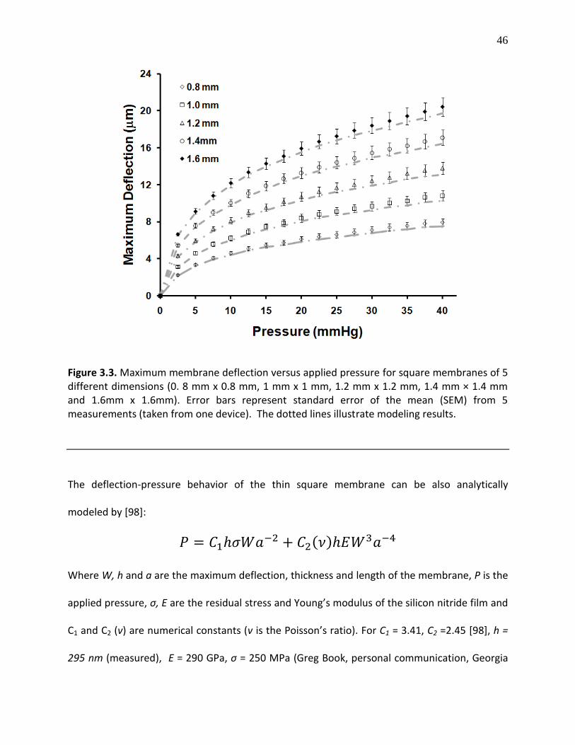
46
Figure 3.3. Maximum membrane deflection versus applied pressure for square membranes of 5 different dimensions (0. 8 mm x 0.8 mm, 1 mm x 1 mm, 1.2 mm x 1.2 mm, 1.4 mm × 1.4 mm and 1.6mm x 1.6mm). Error bars represent standard error of the mean (SEM) from 5 measurements (taken from one device). The dotted lines illustrate modeling results.
The deflection-pressure behavior of the thin square membrane can be also analytically
modeled by [98]:
( )
Where W, h and a are the maximum deflection, thickness and length of the membrane, P is the
applied pressure, σ, E are the residual stress and Young’s modulus of the silicon nitride film and
C1 and C2 (v) are numerical constants (v is the Poisson’s ratio). For C1 = 3.41, C2 =2.45 [98], h =
295 nm (measured), E = 290 GPa, σ = 250 MPa (Greg Book, personal communication, Georgia
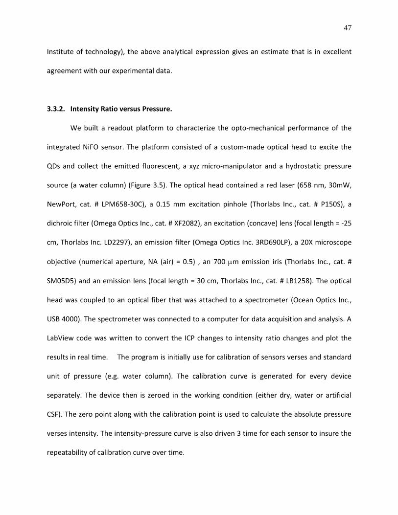
47
Institute of technology), the above analytical expression gives an estimate that is in excellent
agreement with our experimental data.
3.3.2. Intensity Ratio versus Pressure.
We built a readout platform to characterize the opto-mechanical performance of the
integrated NiFO sensor. The platform consisted of a custom-made optical head to excite the
QDs and collect the emitted fluorescent, a xyz micro-manipulator and a hydrostatic pressure
source (a water column) (Figure 3.5). The optical head contained a red laser (658 nm, 30mW,
NewPort, cat. # LPM658-30C), a 0.15 mm excitation pinhole (Thorlabs Inc., cat. # P150S), a
dichroic filter (Omega Optics Inc., cat. # XF2082), an excitation (concave) lens (focal length = -25
cm, Thorlabs Inc. LD2297), an emission filter (Omega Optics Inc. 3RD690LP), a 20X microscope
objective (numerical aperture, NA (air) = 0.5) , an 700 m emission iris (Thorlabs Inc., cat. #
SM05D5) and an emission lens (focal length = 30 cm, Thorlabs Inc., cat. # LB1258). The optical
head was coupled to an optical fiber that was attached to a spectrometer (Ocean Optics Inc.,
USB 4000). The spectrometer was connected to a computer for data acquisition and analysis. A
LabView code was written to convert the ICP changes to intensity ratio changes and plot the
results in real time. The program is initially use for calibration of sensors verses and standard
unit of pressure (e.g. water column). The calibration curve is generated for every device
separately. The device then is zeroed in the working condition (either dry, water or artificial
CSF). The zero point along with the calibration point is used to calculate the absolute pressure
verses intensity. The intensity-pressure curve is also driven 3 time for each sensor to insure the
repeatability of calibration curve over time.

48
Figure 3.5. Schematic of the experimental setup for characterizing the NiFO sensor. The back side of the sensor (chip I) is connected via a plastic tubing to a water column. A similar setup was used to obtain the ‘zero-misalignment’ pressure.
Using the readout platform, we measured the emitted fluorescent intensity at 800 nm
and 705 nm as a function of the applied pressure and calculated the 705 nm / 800 nm intensity
ratio (Figure 3.6A). Membranes of five different dimensions, similar to the ones illustrated in
figure 4, were also tested (Figure 3.6B). To quantify the fluorescent emission intensity for each
QD layer, we calculated the average intensity in the 695 nm - 715 nm and 780 nm – 800 nm
spectral windows for the 705 nm and 800 nm QD layers respectively (see also Figure 3.2).
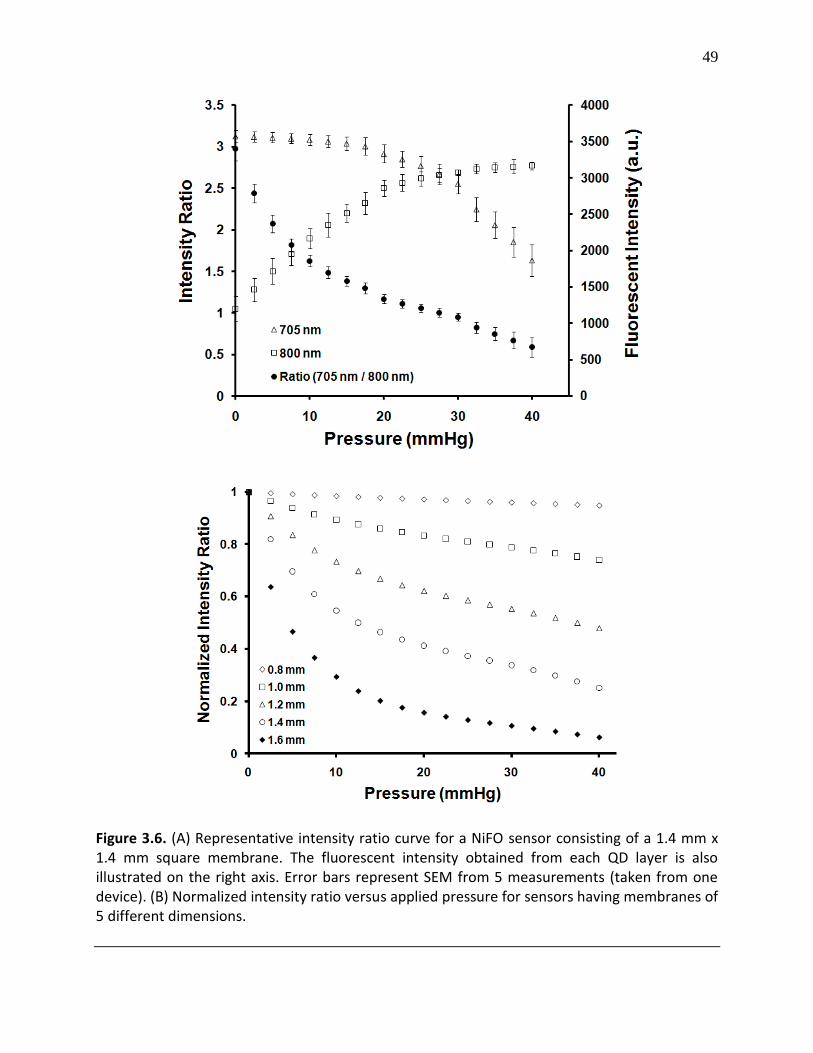
49
Figure 3.6. (A) Representative intensity ratio curve for a NiFO sensor consisting of a 1.4 mm x 1.4 mm square membrane. The fluorescent intensity obtained from each QD layer is also illustrated on the right axis. Error bars represent SEM from 5 measurements (taken from one device). (B) Normalized intensity ratio versus applied pressure for sensors having membranes of 5 different dimensions.
50
For larger membranes (> 1.0 mm x 1.0 mm), the intensity ratio-applied pressure plot
reveals an exponential decay in the 0-20 mmHg regime, while for higher pressure levels (20-40
mmHg) the plot becomes linear (correlation coefficient r = - 0.99). Smaller membranes behave
linearly throughout the entire pressure range (correlation coefficient r = -0.98). The observed
biphasic behavior can be attributed to the biphasic mechanical response of the membrane
(Figure 3.4), as well as to the complex optical interaction of the three-dimensional excitation
focal volume with the two QD layers. We should point out that the dimensions of the excitation
focal volume are determined by the optical properties of the mini-lens (numerical aperture and
depth of field).
The response of the integrated NiFO sensor did not saturate at the maximum applied
pressure of 40 mmHg, indicating that the dynamic range of the sensor is larger than the
pressure range of clinical interest. That is expected if one considers that at 40 mmHg, the 800
nm QD layer is still located within the excitation volume even for the largest membrane
deflection (the depth of field of the excitation volume was measured to be approximately 7
m).
3.3.3. Maximum Error
The maximum error of the NiFO sensor is an important specification as it identifies its overall
performance. The Association for the Advancement of Medical Instrumentation (AAMI) dictates
than an ICP monitoring device should have a maximum error of ± 2mmHg in the range of 0-20
mmHg and 10 % error for higher pressures [77].

51
The maximum error of the sensor can be calculated by adding up the accuracy,
resolution and precision errors. The accuracy error is not significant, as all the NiFO sensors are
calibrated using a hydrostatic water column whose pressure is visually adjusted with an error of
less than 1 mmH20 (equivalent to 0.075 mmHg). The resolution error is also negligible as the
digital output from the spectrometer has a seven decimal digit resolution. The maximum error
is therefore dominated by the precision error (Ep). In our case, the precision error can be
attributed to several factors: optical noise due to random scattering of photons in the various
optical surfaces, laser power instability, thermomechanical vibration of the membrane as well
as electronic noise from the spectrometer.
We calculated the percentage precision error (Ep) that corresponds to a 95% confidence
interval for membranes of 5 different sizes (Figure 3.7). Ep was taken to be two times the
standard deviation (σp) of a set of repeated measurements obtained from the same NiFO
sensor at a given pressure divided by that pressure value (Ep = 2 σp/pressure x 100)). For smaller
membranes, Ep decreases as pressure increases, while for two largest membranes (the 1.4 mm
x 1.4 mm and 1.6 mm x 1.6 mm ones), Ep remains within a 5.5 - 13.8 % range reaching a peak at
20-24 mmHg. Near that peak Ep value, none of the QD layers are in sharp focus (the laser beam
is focused between the two layers) resulting in a weak fluorescent signal from each layer.
Therefore, an intensity ratio with a low signal-to-noise value is obtained that subsequently
increases Ep. The observed peak value is slightly above the threshold error set by the AAMI, but
further design improvements (e.g. spinning multiple layers of QDs to boost the fluorescent
signal) could significantly reduce Ep.

52
Figure 3.7. Percentage precision error (Ep) versus applied pressure. Each Ep value is calculated from 5 measurements taken from a single device (the average of these measurements is depicted in figure 6B). The dotted line illustrates the maximum error set by the Association for the Advancement of Medical Instrumentation (AAMI) for ICP sensors. Large membranes (e.g. the 1.4 mm × 1.4 mm and 1.6mm × 1.6 mm ones) meet the AAMI standards almost through the entire pressure range.
3.3.4. Drift and Photostability of the NiFO sensor
A major concern for chronic ICP monitoring is whether the output signal from the NiFO sensor
is affected by the continuous and long term loading of the membrane as well as the
photobleaching behavior of the QDs. We performed preliminary studies to evaluate: (i) the
midterm (weeks) drift in the optical signal of the NiFO sensor under two loading conditions and
(ii) the photostability of the QD micropillar.
Drift under constant loading. We measured the drift in the intensity ratio from three, 1.4 mm x
1.4 mm, sensors immersed in distilled water for a three week period (Figure 3.8). The devices
were initially bonded at atmospheric pressure and then kept under a constant pressure of 20

53
mmHg and 40 mmHg during the entire experiment. The intensity ratio was recorded every 3
days. The intensity ratio had an average peak-to-peak variation of 6.7 % and 6.8 % at 20 mmHg
and 40 mmHg respectively. The peak-to-peak variation is two times smaller than the precision
error and therefore, no significant drift was observed. It is possible that the in vivo environment
might alter the mechanical behavior of the membrane e.g. due to the accumulation of brain
tissue at the surface of the nitride membrane, but such experiments are beyond the scope of
this work.
QD Trilayer Photostability. The photostability of QDs is essential for the long-term operation of
the NiFO sensor. Despite the fact that QDs do not photobleach [99] when compared to
traditional fluorescent dyes that used for biological imaging, their photoluminescent properties
strongly depend on the surrounding material and environmental conditions [97, 100,101] .
To study the photostability of the QDs, we prepared two silicon nitride membranes with
a 705 nm QD layer and a 800 nm QD/ layer respectively. A 2 m thick SU-8 layer, representing
the optical spacer, was spun on top of each membrane to entirely cover each QD layer. The QD
coated membranes were illuminated with a red laser (658 nm) at an optical power density of
0.75 W/cm2 and the change of fluorescent intensity as well as the maximum emission
wavelength were recorded over a period of 200 min of continuous exposure (Figure 3.9). An
increase in the laser power by a factor of 2 did not change the fluorescent intensity, indicating
that the initial power density of 0.75 W/cm2 was enough to saturate the QD signal. No blinking
was observed, as individual QDs could not be resolved due to the low resolution of the mini-
lens.
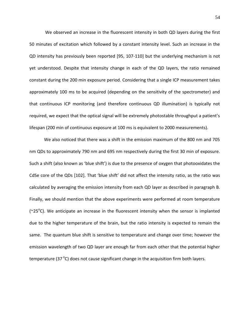
54
We observed an increase in the fluorescent intensity in both QD layers during the first
50 minutes of excitation which followed by a constant intensity level. Such an increase in the
QD intensity has previously been reported [95, 107-110] but the underlying mechanism is not
yet understood. Despite that intensity change in each of the QD layers, the ratio remained
constant during the 200 min exposure period. Considering that a single ICP measurement takes
approximately 100 ms to be acquired (depending on the sensitivity of the spectrometer) and
that continuous ICP monitoring (and therefore continuous QD illumination) is typically not
required, we expect that the optical signal will be extremely photostable throughput a patient’s
lifespan (200 min of continuous exposure at 100 ms is equivalent to 2000 measurements).
We also noticed that there was a shift in the emission maximum of the 800 nm and 705
nm QDs to approximately 790 nm and 695 nm respectively during the first 30 min of exposure.
Such a shift (also known as ‘blue shift’) is due to the presence of oxygen that photooxidates the
CdSe core of the QDs [102]. That ‘blue shift’ did not affect the intensity ratio, as the ratio was
calculated by averaging the emission intensity from each QD layer as described in paragraph B.
Finally, we should mention that the above experiments were performed at room temperature
(~25oC). We anticipate an increase in the fluorescent intensity when the sensor is implanted
due to the higher temperature of the brain, but the ratio intensity is expected to remain the
same. The quantum blue shift is sensitive to temperature and change over time; however the
emission wavelength of two QD layer are enough far from each other that the potential higher
temperature (37 oC) does not cause significant change in the acquisition firm both layers.
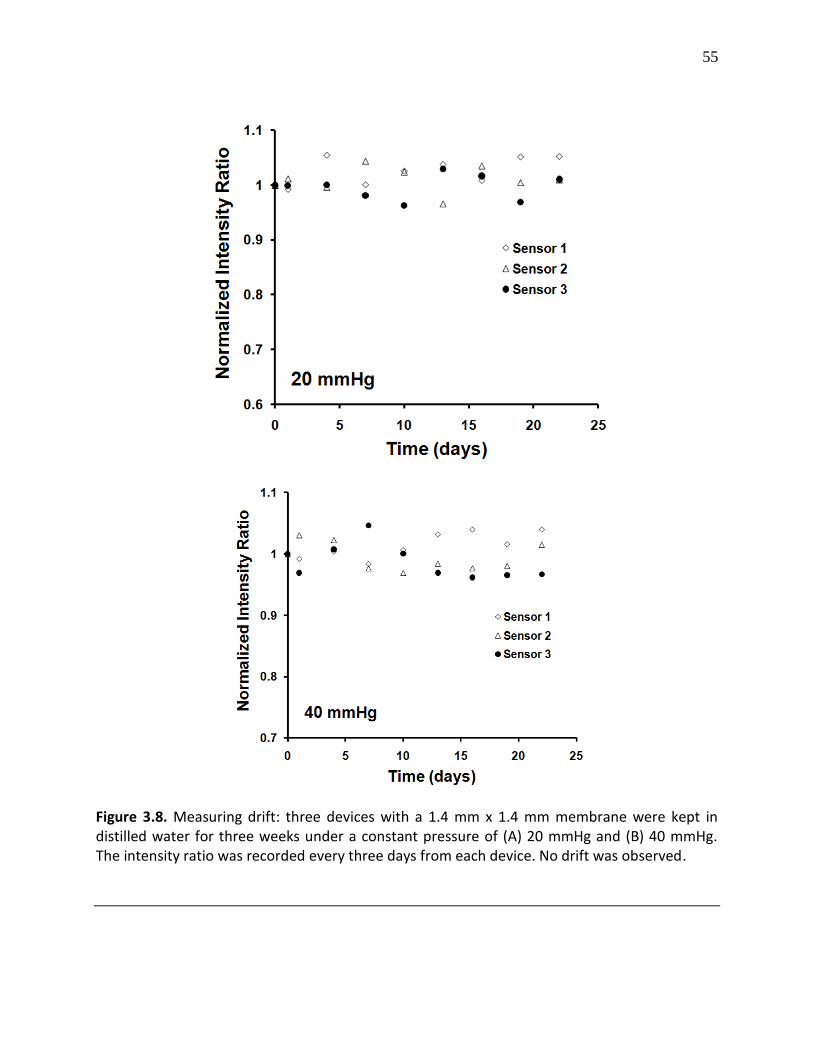
55
Figure 3.8. Measuring drift: three devices with a 1.4 mm x 1.4 mm membrane were kept in distilled water for three weeks under a constant pressure of (A) 20 mmHg and (B) 40 mmHg. The intensity ratio was recorded every three days from each device. No drift was observed.
56
3.3.5. ‘Zero-Misalignment’ Pressure
Due to variations in the fabrication process (e.g. wafer thickness, QD micropillar
thickness, mini-lens diameter and focal length) the collimated excitation beam entering the
NiFO sensor is not accurately focused at the 705 nm QD layer of the QD micropillar at zero
pressure, as initially designed. We found that the distance (z-axis misalignment) between the
705 nm QD layer and the focal plane of the mini-lens was 4-5 m and varied from device to
device. In order to obtain a common reference point for all tested devices, we measured that
‘focal plane to the 705 nm QD layer’ distance using an optical setup similar to the one depicted
in figure 5. We followed a 5-step experimental procedure : (i) the excitation lens was initially
removed from the original optical setup such that the laser beam when reaching the mini-lens
was slightly focused, (ii) using a CCD camera, the 705 nm QD layer was brought into sharp focus
(the spectrometer was replaced with the CCD in this step in order to accurately position the 705
nm QD layer at the focal plane of the mini-lens), (iii) the 705 nm / 800 nm intensity ratio was
recorded at this position using the spectrometer, (iv) the excitation lens was placed back into
the setup (in front of the laser) so that that laser beam reaching the NiFO device was
collimated, and (v) hydrostatic pressure was applied to the membrane while the intensity ratio
was recorded.

57
Figure 3.9. Photostability of the QD micropillar for different laser power densities. QD micropillars were patterned on a silicon nitride membrane and were continuously exposed with a red (658 nm) laser for more than 2 h. (a) Normalized fluorescent intensity obtained from the 705 nm QD layer. (b) Normalized fluorescent intensity obtained from the 800 nm QD layer. (c) Normalized intensity ratio (705 nm/800 nm) calculated from (a) and (b). Despite the initial increase in the intensity in both QD layers, the intensity ratio remained constant after the initial “burning” period (peak-to-peak value was less than 1% after 60 min of continuous exposure).
A hydrostatic pressure of 1-3 mmHg (termed ‘zero-misalignment’ pressure) was
sufficient to match the intensity ratio to the one obtained from step (iii) (without using the
diverging lens). All experimental results in Figures 3.6 and 3.7 were corrected accordingly using
that ‘zero-misalignment’ pressure.
3.3.6. Effect of Skin on the performance of the NiFO sensor
58
As the NiFO sensor is designed for implantation inside the brain using a hollow tube that
is placed under the skin (Figure 3.1A), we anticipate that the NI optical properties and the
thickness of the skin will affect the intensity of the excitation and emitted light. To evaluate the
effect of skin at the performance of the NiFO sensor, we used a commercially available Monte
Carlo Simulation software [103] to trace the trajectories of photons as they pass and scatter
through the skin. The skin was modeled as a single optical layer with a reduced scattering and
absorption coefficient of μs’= 210 cm-1 and μa= 1.5 cm-1 respectively [103-105]. The simulation
model (Figure 3.10A) consisted of a 20 m in diameter laser beam that entered the skin
collimated, a 500 m square silicon nitride optical window (100% transparency in the NI) and
the mini-lens that focused the laser beam into the QD micropillar. Following a similar light path,
the emitted NI fluorescence light exited the 500 m optical window of chip III collimated, and
after passing the skin, was scattered and collected by an external bi-convex lens (the lens was
assumed to have 1 cm diameter and a focal length of 25 mm).
The Monte Carlo results indicated that the laser power that reaches the NiFO sensor
collimated is significantly reduced due to the high scattering coefficient of the skin (Figure
3.10B). For the extreme case of a 2 mm thick skin (typically skin in the scalp is 0.5 -1.5 mm thick
[105]), our simulation results indicate that approximately 1% of the laser power enters the NiFO
sensor collimated. The reduced excitation power can be compensated by increasing the laser
power, as long as skin damage does not occur (the maximum laser limit for low level laser
therapy set by the AAMI is 5 W/cm2 [106]). The emitted fluorescent light is also highly scattered
as it passes through the skin.

59
Simulations show that, for a 2 mm thick skin layer, only 1% of the fluorescence light
exits the skin collimated (87% is being scattered). Although our current experimental setup
measures collimated light (only collimated light is focused into the spectrometer), further
design modifications can be made to utilize the scattered light as the 705 nm / 800 nm ratio of
the scattered fluorescent light should be the same as the collimated one. Finally, we should
point out that the amount of the detected emitted light depends on the sensitivity of the
spectrometer. The use of a two-detector configuration (e.g. using two avalanche photodiodes
[107] would greatly enhance the overall sensitivity of the system.
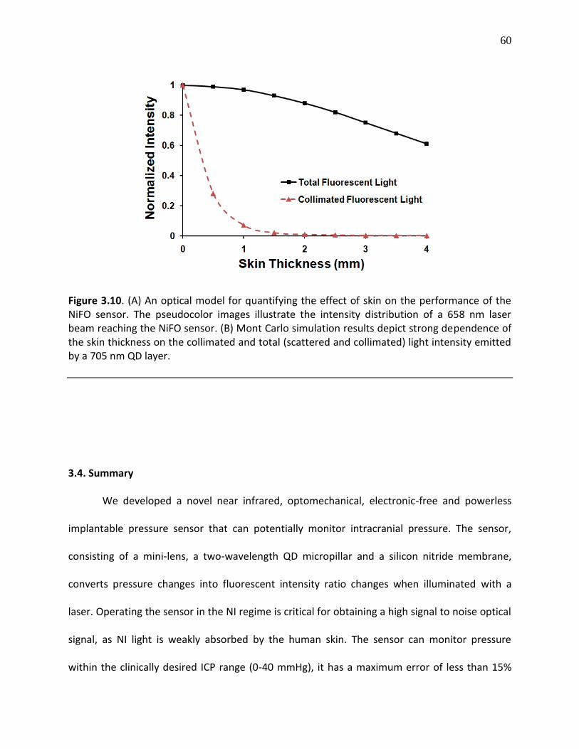
60
Figure 3.10. (A) An optical model for quantifying the effect of skin on the performance of the NiFO sensor. The pseudocolor images illustrate the intensity distribution of a 658 nm laser beam reaching the NiFO sensor. (B) Mont Carlo simulation results depict strong dependence of the skin thickness on the collimated and total (scattered and collimated) light intensity emitted by a 705 nm QD layer.
3.4. Summary
We developed a novel near infrared, optomechanical, electronic-free and powerless
implantable pressure sensor that can potentially monitor intracranial pressure. The sensor,
consisting of a mini-lens, a two-wavelength QD micropillar and a silicon nitride membrane,
converts pressure changes into fluorescent intensity ratio changes when illuminated with a
laser. Operating the sensor in the NI regime is critical for obtaining a high signal to noise optical
signal, as NI light is weakly absorbed by the human skin. The sensor can monitor pressure
within the clinically desired ICP range (0-40 mmHg), it has a maximum error of less than 15%

61
and it does not suffer from photobleaching and drift. We envision that the proposed near
infrared fluorescent-based optomechanical (NiFO) sensing technology can be extended to other
biomedical applications where in vivo pressure monitoring is required such as arterial,
intraocular and gastrointestinal pressure monitoring.
62
CHAPTER 4
IMPLANTABLE INTRAOCULAR PRESSURE SENSOR: EX VIVO STUDIES
4.1. Introduction
One of them most common forms of neuronal injury, only second to the traumatic brain
injury is the optical nerve damage. Pathological conditions (e.g. elevated intraocular
pressure) can induce mechanical damage to optical nerve resulting in permanent blindness.
Intraocular pressure (IOP) monitoring is as an essential diagnostic tool for assessing and
treating the patients with glaucoma (normal IOP ranges from 7-15 mmHg). High intraocular
pressure (IOP), the major risk factor for glaucoma, is the leading cause of blindness in the
aging population [111]. IOP monitoring followed by the appropriate medical treatment
dramatically reduces the number of blindness, minimizes secondary optical nerve damage
and significantly decreases recovery time after surgery.
There is no commercial technology that can provide continuous monitoring. Such
technology is needed: (i) for patients that suffer from severe cases of glaucoma that
typically are hospitalized for several days, and (ii) for patients who go though surgery with
high chance of glaucoma as a side effect of surgery. In the latter case, long time IOP
monitoring can aid in the diagnosis of a surgical side effect particularly in the patient with
ocular implants.
Current IOP assessment, since their introduction in the early 60’s, has undergone few
design changes and remains cumbersome in placement and use. The basic operation
principle has remained the same: a pin containing a pressure sensor is touching the surface
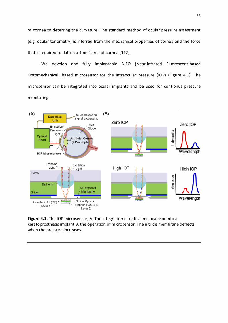
63
of cornea to deterring the curvature. The standard method of ocular pressure assessment
(e.g. ocular tonometry) is inferred from the mechanical properties of cornea and the force
that is required to flatten a 4mm2 area of cornea [112].
We develop and fully implantable NiFO (Near-infrared Fluorescent-based
Optomechanical) based microsensor for the intraocular pressure (IOP) (Figure 4.1). The
microsensor can be integrated into ocular implants and be used for contionus pressure
monitoring.
Figure 4.1. The IOP microsensor, A. The integration of optical microsensor into a keratoprosthesis implant B. the operation of microsensor. The nitride membrane deflects when the pressure increases.

64
4.2. Method
4.2.1. Design and fabrication
We present a new implantable electronic-free, fully optical intraocular pressure
microsensor, designed to be embedded into a KPro implant (Figure 4.1A). The microsensor
contains 2 layers of infrared quantum dots (QD) (emitting 850 nm and 920 nm florescent
light), patterned on top a 300nm thick silicon nitride membrane that is exposed to IOP. A
400 µm in diameter sapphire lens is placed 370µm above the QDs and secured in with a
layer of PDMS (Figure 4.2). The lens focuses collimated excitation light to the QD layers and
collects the fluorescent emitted light. When the membrane is flat, the 850 nm QD layer is in
focus, e.g. at the focal plane of the lens. A pressure increase deflects the membrane brings
the 920nm QD layer closer to the focal plane while the 800 nm QD layer moves away from
the focal plane of the lens (Figure 4.1B). To read the sensor, we designed an optical head to
excite the QD layers using a 65mW 780nm laser and collect the fluorescent emission from
the focal plane of the microlens (Figure 4.1C). The collected optical signal then is processed
using a set of filters that separate the two wavelengths to find the ratio of 920nm and
850nm emission intensity. We then calibrate the obtained ratio (920nm/850nm) with
respect to a known external pressure (Figure 4.3A). Later, for biocompatibility 500nm
parylene layer is deposited on the device. The simulation (Figure 4.3B) and experimental
results (Figure 4.4) show less than 5% change in the response of sensor due to protective
layer.

65
Figure 4.2. The NiFO sensor consists of a chip, with a micorlens manually assembled on top
of it.The chip has a transparent, 150 nm thick silicon nitride membrane. The key element of
the design, the QD micropillar, consists of two QD layers and two SU8 layers that are
photolithographically patterned on top of the IOP-exposed membrane.
4.2.2. Keratoprosthesis device implant
Keratoprosthesis (KPro) surgery has provided a new chance, over the past 2 decades for
patients with corneal impairment, who otherwise would not be suitable candidates for
traditional penetrating keratoplasty [111-114]. The recent techniques and postoperative
regimen modifications have improved the prognosis after KPro surgery [111,114, and 115].
However, one main issue with all types of KPro remains unsolved: about 64% of patients
show decreased vision due to glaucoma development postoperatively [111, 112, and 114-
117]. The onset and progression of glaucoma in these patients are very critical for successful
recovery from the surgery [112, 118].

66
Particularly, in patients with ocular implants such as Keratoprosthesis (KPro) [113],
with very high glaucoma prevalence, tonometry method is not applicable (Figure 4.2). For
example, the KPro implant, placed on under cornea, increases the mechanical stiffness of
tissue, and makes tonometry method readings invalid.
Figure 4.3. A. Ratio between 850nm channel and 920nm verse pressure in mmHg. The ratio is used to calibrate each microsensor separately. B. Simulation result for the membrane with parylene deposition. The simulation suggests 500nm of paraylene deposition change the deflection less than 5%.
Figure 4.4. Effect of Parylene deposition on the optical readout of the pressure. To protect the surface of the surface 500nm parylene is deposited in the holder and microsensor. The experimental result should less than 5% change in the calibration curve.

67
Despite the high prevalence of glaucoma in the post KPro implant surgery, no
reliable ocular pressure monitoring method for glaucoma risk determination for implant
patient is available [119-121]. The major issue is the standard cornea deflection base IOP
assessment is not possible in present of inflexible KPro material supporting the cornea [112,
116, and 119].
The microsensor is integrated into the Boston type 1 keratoprosthesis (KPro) and
implanted into human cadaver globe. We implant KPro with an integrated NiFO microsensor
in 5 human eye globes and measure the pressure over a period of two weeks. The result
shows consistent operation of sensor with 2mmHg accuracy over 14-days period without a
zero-drift.
Motivated by the need for frequent, long-term IOP monitoring in patients with KPro
implants, we developed an IOP microsensor, designed to be embedded into the KPro device
and implant at the time of surgery. The new microsensor could reduce the risk of glaucoma
late diagnosis in patients with ocular implant, and partially in patients with KPro implant.
The microsensor has a diameter of 1.15 mm, slightly bigger than circular fluidic holes
in the KPro device (diameter of 1.1mm). The KPro device gently expands when heated to
90oC. That allows us to insert the microsensor into one of the KPro holes. Finally the
integrated unit is cooled down to room temperature to obtain a tight fit (Figure 4.6A).
When the membrane is flat (zero IOP), the 850 nm QD layer is in focus, i.e. at the
focal plane of the lens. A pressure increase deflects the membrane bringing the 920 nm QD
layer closer to the focal plane of the lens, while the 800 nm QD layer moves away from it
(Figure 4.2C). To read the sensor, an optical head was designed to excite the QD layers using

68
a 65 mW 780 nm laser and collect the fluorescent emission from the focal plane of the
microlens (Figure 4.3). The collected optical signal then is processed using a set of filters
(dichroic and achromatic lens) that separate the two wavelengths to find the ratio of 920
nm and 850nm emission intensity. The obtained ratio (920 nm/850 nm) is then calibrated
with respect to a known external pressure.
Figure 4.5. keratoprosthesis implant, A. the KPro device is consist of 3 parts Back Plate, Locking Ring and Front Part assemble into a Corneal Graft (image is adapter from eyeworld.org), B. the KPro device assembled with Corneal Graft (image is adapter from eyeworld.org), C. KPro device after implantation into human globe (image is adapter from eyeworld.org), D. Implantation and sealing process (image is adapter from [112]).
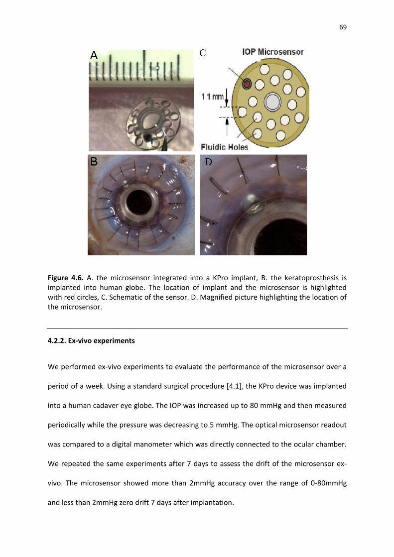
69
Figure 4.6. A. the microsensor integrated into a KPro implant, B. the keratoprosthesis is implanted into human globe. The location of implant and the microsensor is highlighted with red circles, C. Schematic of the sensor. D. Magnified picture highlighting the location of the microsensor.
4.2.2. Ex-vivo experiments
We performed ex-vivo experiments to evaluate the performance of the microsensor over a
period of a week. Using a standard surgical procedure [4.1], the KPro device was implanted
into a human cadaver eye globe. The IOP was increased up to 80 mmHg and then measured
periodically while the pressure was decreasing to 5 mmHg. The optical microsensor readout
was compared to a digital manometer which was directly connected to the ocular chamber.
We repeated the same experiments after 7 days to assess the drift of the microsensor ex-
vivo. The microsensor showed more than 2mmHg accuracy over the range of 0-80mmHg
and less than 2mmHg zero drift 7 days after implantation.

70
Five cadaver human eye globes and 5 corneal rims, not suitable for transplant
criteria, were donated by the Midwest Eye-Banks (Ann Arbor, MI, USA) for this study. The
NiFO IOP sensor, designed to fit tightly into one of the Boston type 1 KPro posterior plate
holes, was integrated after KPro was heated up to 90oC, to slightly expend. As it returned to
the room temperature, the sensor was secured in the hole.
KPro implantation was performed via the standard technique [4.12], at the W. K.
Kellogg Eye Center Department of Ophthalmology, University of Michigan Medical School
(Ann Arbor, MI, USA) (Figure 4.6B, C). After making a paracentesis, with a lancetip blade, at
a clear cornea portion of the host globe, an anterior chamber cannula, which was connected
to a digital manometer (Digimano 1000, Netech Corp., Farmingdale, NY, USA), was inserted
(Figure 4.7). The eye globe was inflated, then, by an irrigation cannula and a 10 ml syringe
filled with BSS, through the corneal graft dehiscence, until it started leaking out (considered
maximum volume). Using an external optical head reader, the NiFO IOP sensor output was
compared simultaneously with the digital manometer, considered a standard measurement.
The internal structure of NiFO optical head is shown in Figure 4.8.
Readings were recorded immediately after the KPro implantation and after 1 week
for all the 5 globes (Table 1). For one microsensor the readouts were extended up to 14
days. The globes were maintained in refrigeration (4oC) between the measurements and
then discarded in an appropriate biohazard bucket after the final IOP readings. The IOP
measurement characteristics evaluated were accuracy (resolution) and consistency (drift)
through regression statistics tests, such as the Standard error and R factor.

71
Figure 4.7. IOP Measurement setup, A. Optical head, B. Digital pressure monitor directly connected to ocular chamber. C. schematic of the setup, the globe is filled with saline solution and the pressure increased to 80mmHg. As pressure decreases the reading from digital sensor is compare to optical head readout form NiFO microsensor.
4.3. Results
NiFO IOP sensor readings and the digital manometer readings are shown in Figure 4.10. The
globes are inflated to 80mmHg by injecting the DI water. In the first day, the issue was fresh
so the seal of KPro device could hold high pressure. Initially the pressure dropped very fast
to 40mmHg (the high range physiological pressure). The pressure is then decreased using a
needle. Uniformly distributed pressure measures are collected in the first day. After 7 days,
the deteriorated tissues did not hold the pressure, so in some cases (sensor 1 and 4) the
distribution of the pressure samples was not uniform. We calculate the correlation between
optical readout and direct pressure measurement using manometer. The linear correlation
indicates the proper calibration of the optical sensor. Our results show all sensors are still
calibrated after 7 days of implantation (Figure 4.9, Table 3). While the microsensor was
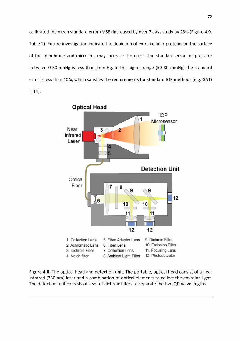
72
calibrated the mean standard error (MSE) increased by over 7 days study by 23% (Figure 4.9,
Table 2). Future investigation indicate the depiction of extra cellular proteins on the surface
of the membrane and microlens may increase the error. The standard error for pressure
between 0-50mmHg is less than 2mmHg. In the higher range (50-80 mmHg) the standard
error is less than 10%, which satisfies the requirements for standard IOP methods (e.g. GAT)
[114].
Figure 4.8. The optical head and detection unit. The portable, optical head consist of a near infrared (780 nm) laser and a combination of optical elements to collect the emission light. The detection unit consists of a set of dichroic filters to separate the two QD wavelengths.

73
Our results suggest that the accuracy of the microsensor (2mmHg) is comparable to
standard tonometry procedure; therefore our microsensor can reliably monitor IOP in
glaucoma patients where the standard method is not applicable. The results also indicate
the potential use of such an optomechanical technology for long-term in-vivo IOP
monitoring.
4.4. Discussion and Summary
All 5 transducers demonstrated a very linear results pattern between both optical and
manometric readings (Figure 4.9), even after 14 days of KPro/NiFO IOP sensor implantation
(sensor 1). On the other hand, the sample distribution was not homogeneous, because of
the eye tissue natural degeneration, which can be noticed, e.g., on the 7th day of sensors 3
and 4, where there are a lot data collected at higher IOP ranges. Since the transducer is
calibrated to function between 0 to 50 mmHg, these particular transducers resulted larger
errors, attributed to the higher ratios between the 2 near-infrared wavelength fluorescent
lights at the end.
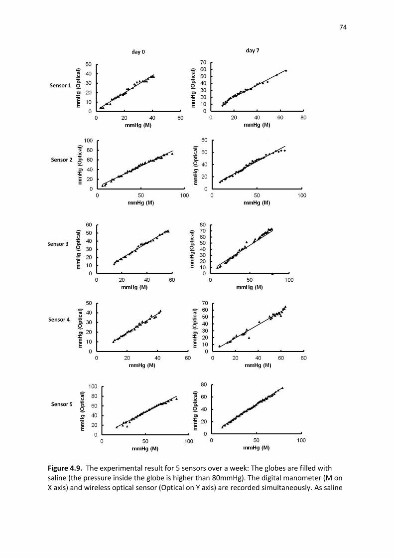
74
Figure 4.9. The experimental result for 5 sensors over a week: The globes are filled with saline (the pressure inside the globe is higher than 80mmHg). The digital manometer (M on X axis) and wireless optical sensor (Optical on Y axis) are recorded simultaneously. As saline
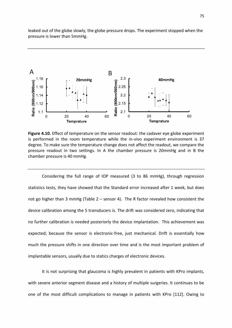
75
leaked out of the globe slowly, the globe pressure drops. The experiment stopped when the pressure is lower than 5mmHg.
Figure 4.10. Effect of temperature on the sensor readout: the cadaver eye globe experiment is performed in the room temperature while the in-vivo experiment environment is 37 degree. To make sure the temperature change does not affect the readout, we compare the pressure readout in two settings. In A the chamber pressure is 20mmHg and in B the chamber pressure is 40 mmHg.
Considering the full range of IOP measured (3 to 86 mmHg), through regression
statistics tests, they have showed that the Standard error increased after 1 week, but does
not go higher than 3 mmHg (Table 2 – sensor 4). The R factor revealed how consistent the
device calibration among the 5 transducers is. The drift was considered zero, indicating that
no further calibration is needed posteriorly the device implantation. This achievement was
expected; because the sensor is electronic-free, just mechanical. Drift is essentially how
much the pressure shifts in one direction over time and is the most important problem of
implantable sensors, usually due to statics charges of electronic devices.
It is not surprising that glaucoma is highly prevalent in patients with KPro implants,
with severe anterior segment disease and a history of multiple surgeries. It continues to be
one of the most difficult complications to manage in patients with KPro [112]. Owing to
76
KPro´s material stiffness, for the time being, clinicians remain dependent on palpation to
monitor IOP, which is not objective and has poor correlation with the Goldmann
applanation tonometer (GAT). This may collaborate to glaucoma progression.
However, the NiFO IOP sensor presents special features make it unique and innovative. It is
wireless, purely optical and powerless. Specifically designed to be embedded with the KPro
device, it provides an integrated solution for IOP monitoring without changing the KPro
implantation procedure. It also allows frequent measurements and recordings of the direct
measure (“true” IOP) rather than GAT that gives only an indirect measure of IOP in addition
to being interfered from changes in corneal features.
With no contact with the cornea, topical anesthesia is no more required and the risk
of cross-infection between patients no longer exits. Moreover, it does not cause visual field
intervention and is MRI compatible. The silicon nitride, used on each layer, is also
transparent and biocompatible as glass (silicon oxide). The developed optical head can read
up to 4 measurements per second. Blood and myelin have a very low absorption of the
near-infrared light, allowing its transmission, what could mean that even after a graft
failure, with edematous and/or opaque cornea, it will continue to transmit information.
In contrast, the study, and likewise the microsensor, has limitations. The data
collected was not uniform, as mentioned. This device has a very specific application, limiting
the population to be assisted. Biocompatibility still has to be tested on future animal trials.
Besides, the American National Standard, related to the Association for the Advancement of
Medical Instrumentation has no protocol for IOP devices, what makes it harder to unify the
transducer features. The results suggest that this novel fully implantable and pure optical
transducer, through a direct IOP measurement, may allow objective and reliable
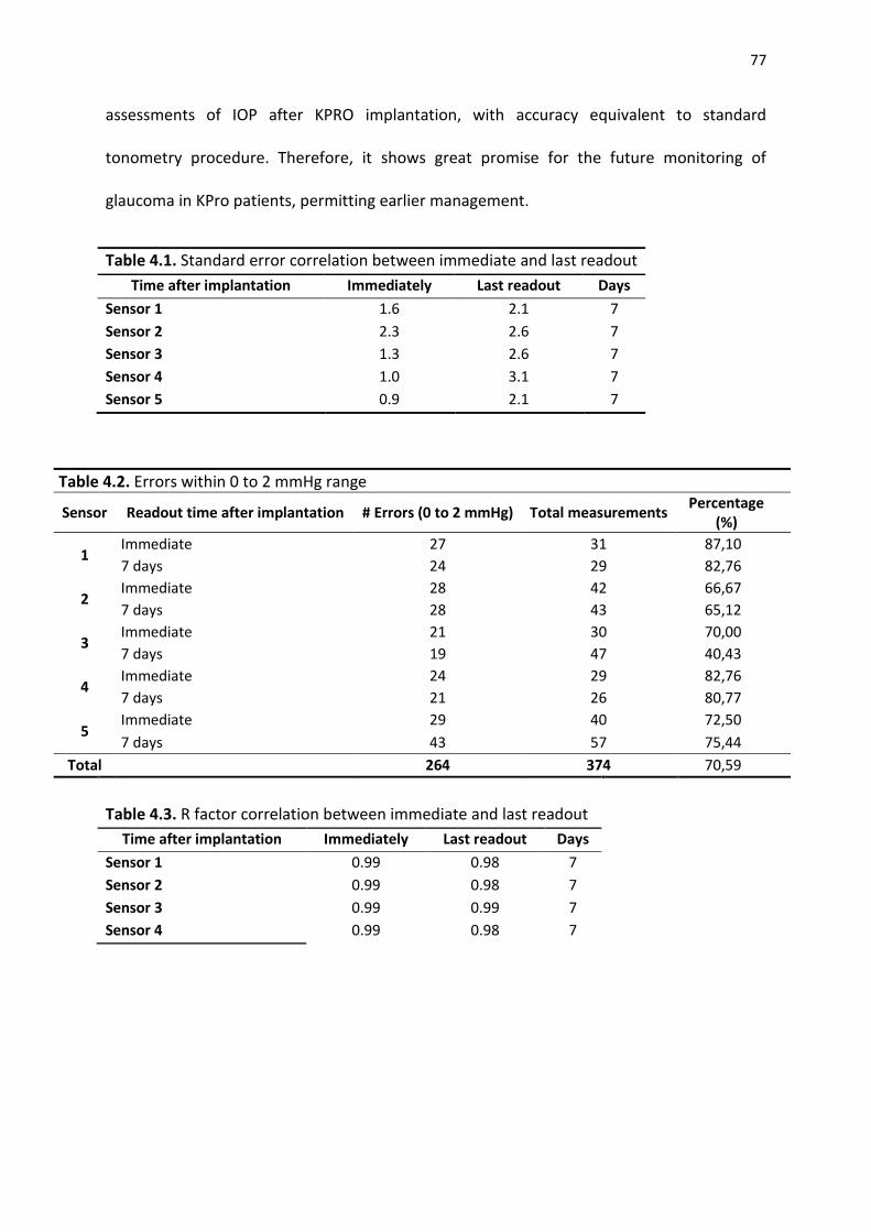
77
assessments of IOP after KPRO implantation, with accuracy equivalent to standard
tonometry procedure. Therefore, it shows great promise for the future monitoring of
glaucoma in KPro patients, permitting earlier management.
Table 4.1. Standard error correlation between immediate and last readout
Time after implantation Immediately Last readout Days
Sensor 1 1.6 2.1 7
Sensor 2 2.3 2.6 7
Sensor 3 1.3 2.6 7
Sensor 4 1.0 3.1 7
Sensor 5 0.9 2.1 7
Table 4.2. Errors within 0 to 2 mmHg range
Sensor Readout time after implantation # Errors (0 to 2 mmHg) Total measurements Percentage
(%)
1 Immediate 27 31 87,10
7 days 24 29 82,76
2 Immediate 28 42 66,67
7 days 28 43 65,12
3 Immediate 21 30 70,00
7 days 19 47 40,43
4 Immediate 24 29 82,76
7 days 21 26 80,77
5 Immediate 29 40 72,50
7 days 43 57 75,44
Total
264 374 70,59
Table 4.3. R factor correlation between immediate and last readout
Time after implantation Immediately Last readout Days
Sensor 1 0.99 0.98 7
Sensor 2 0.99 0.98 7
Sensor 3 0.99 0.99 7
Sensor 4 0.99 0.98 7

78
CHAPTER 5
IN-VIVO IMPLANTATION OF OPTICAL SENSOR IN SHEEP MODEL
5.1. Introduction
In this chapter,the NiFO sensor performance was evaluated in-vivo. We assessed the agreement
between theNiFO microsensor and a standard ICP monitor (Codman microsensor) during a
standard ICP sensor implantation method in a sheep brain [122]. The Codman microsensor, a
catheter-based sensor that is hard-wired to a benchtop electronic readout unit, is currently the
gold standard for human ICP monitoring.
Two cross-bred sheep were used in our in vivo study. The cranium of anesthetized sheep
was exposed by a paramedian incision and 2 adjacent burr holes were drilled over the frontal
lobe. The Codman microsensor were inserted into the parenchyma through one hole and a
NiFO sensor was inserted through the other hole. The Codman microsensor was connected to
the monitoring unit via the appropriate interface. The NiFO sensor was fully implanted as the
ICP signal is optically transmitted through the skin.
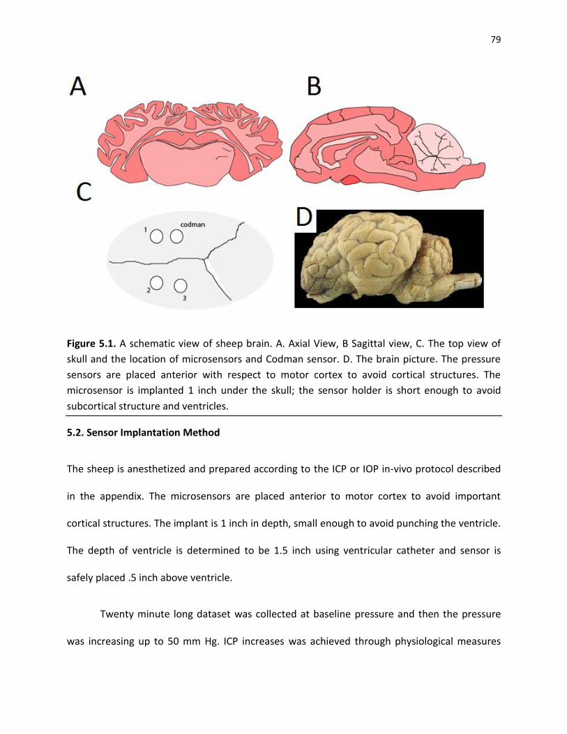
79
Figure 5.1. A schematic view of sheep brain. A. Axial View, B Sagittal view, C. The top view of
skull and the location of microsensors and Codman sensor. D. The brain picture. The pressure
sensors are placed anterior with respect to motor cortex to avoid cortical structures. The
microsensor is implanted 1 inch under the skull; the sensor holder is short enough to avoid
subcortical structure and ventricles.
5.2. Sensor Implantation Method
The sheep is anesthetized and prepared according to the ICP or IOP in-vivo protocol described
in the appendix. The microsensors are placed anterior to motor cortex to avoid important
cortical structures. The implant is 1 inch in depth, small enough to avoid punching the ventricle.
The depth of ventricle is determined to be 1.5 inch using ventricular catheter and sensor is
safely placed .5 inch above ventricle.
Twenty minute long dataset was collected at baseline pressure and then the pressure
was increasing up to 50 mm Hg. ICP increases was achieved through physiological measures
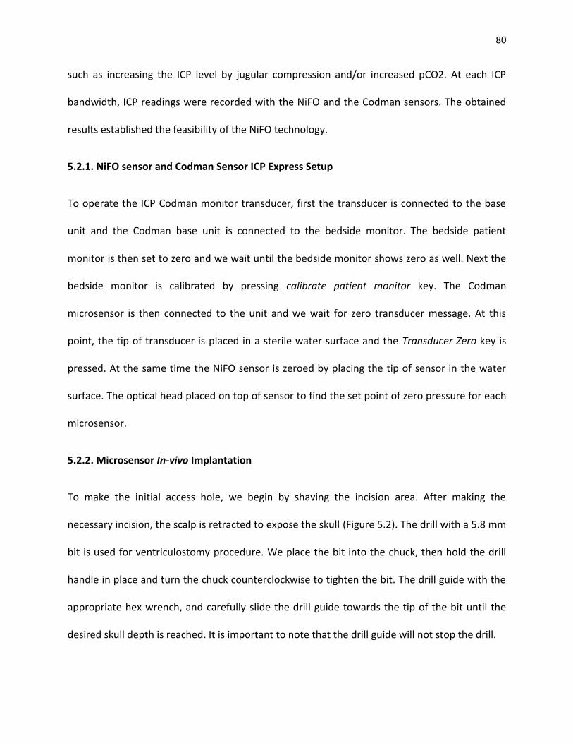
80
such as increasing the ICP level by jugular compression and/or increased pCO2. At each ICP
bandwidth, ICP readings were recorded with the NiFO and the Codman sensors. The obtained
results established the feasibility of the NiFO technology.
5.2.1. NiFO sensor and Codman Sensor ICP Express Setup
To operate the ICP Codman monitor transducer, first the transducer is connected to the base
unit and the Codman base unit is connected to the bedside monitor. The bedside patient
monitor is then set to zero and we wait until the bedside monitor shows zero as well. Next the
bedside monitor is calibrated by pressing calibrate patient monitor key. The Codman
microsensor is then connected to the unit and we wait for zero transducer message. At this
point, the tip of transducer is placed in a sterile water surface and the Transducer Zero key is
pressed. At the same time the NiFO sensor is zeroed by placing the tip of sensor in the water
surface. The optical head placed on top of sensor to find the set point of zero pressure for each
microsensor.
5.2.2. Microsensor In-vivo Implantation
To make the initial access hole, we begin by shaving the incision area. After making the
necessary incision, the scalp is retracted to expose the skull (Figure 5.2). The drill with a 5.8 mm
bit is used for ventriculostomy procedure. We place the bit into the chuck, then hold the drill
handle in place and turn the chuck counterclockwise to tighten the bit. The drill guide with the
appropriate hex wrench, and carefully slide the drill guide towards the tip of the bit until the
desired skull depth is reached. It is important to note that the drill guide will not stop the drill.

81
To measure ICP via the intraparenchymal approach, begin with the Codman micro sensor
already zeroed. We then create the burr hole through which the micro sensor will be placed,
with the 2.7 mm drill bit. Bevel the Burr Hole edge on the side where the microsensor will exit.
This will facilitate remove of the sensor.
Figure 5.2. Candman and NiFO sensor implantation procedure. A. drilling the 5.8 mm hole in
the anterior to motorcortext, B. drilling parallel holes for Codman sensor, C. end of procedure
with three NiFO sensor and one Codman sensor implantation, D. Closing the skin
We then remove the Touhy needle stylet and thread the microsensor from the top of
the needle until appropriate length of placement exits from the hub. Then, gently we remove
the needle and estimate the length of the micro sensor from the tip to the fist kink. Once again,
we retract the Burr Hole site. We then fold the microsensor forward once at the desired bend

82
site to leave a kink in it. Then we place the tip of microsensor in the Parenchyma through the
puncture in the Dura until the kink is at the top edge of the hole. We pull back the excess slack
and secure the microsensor to the scalp. For additional strain relief, we made a small loop with
the line and suture to down.
5.2.3. Measuring Intracranial Pressure
To measure intracranial pressure, we begun with the microsensor already zeroed. To perform
the craniostomy, we use a 5.8mm drill bit. Gently, we bevel the Burr Hole on the side where the
catheter exit site will be. Then we make a cruciate puncture in the Dura. We placed the
Ventricular Catheter in the trocar tube and tunnel it under scalp from the exit site toward the
Burr Hole. Finally we remove the trocar. The 10 gauge ventricular needle is used to locate the
ventricle first. The catheter is advanced into the lateral ventricle and make sure to enter the
skull at a right angle. We verify that the tip of the ventricular catheter is situated in the ventricle
by removing the capon the drain port and allowing CFS to flow out and then we drain the port.
Then we bend the catheter in place and gently withdraw the preloaded stylet.
5.2.3. Closing the incision
After the placing the microsensors, the providing access to Codman sensor, the optical data is collected
first with open skin. All data are collected for 30 sec or more. The skin then is closed and another set of
data is collected. The skin is closed very carefully to avoid Codman microsensor movement.
5.2.4. Testing the dynamic range of microsensor in vivo
83
The procedure to test the dynamic range of pressure sensor has 7 phases and is designed to
test the dynamic range 0-50mmHg of pressure in-vivo using non-invasive and invasive
approaches.
1. The pressure is monitored in the baseline breathing rate of 15 breaths/min for 20
minutes. The ICP pressure oscillates between systolic and diastolic cycles (about 2mmHg
difference between maximum and minimum pressure) with the average of 18mmHg. In
clinic, the oscillation usually is monitoring to verify the pressure sensor proper
operation. The total volume of lung is set to 500ml.
2. To observe the maximum change in ICP pressure, we need to decrease ICP. For this, the
breathing rate is increased to 30 breaths/min, the lung volume remain at 500ml. After 5
minutes the intracellular oxygen increased for 10% and the ICP average decreases to 12
mmHg. At this point brain pressure auto regulation mechanism maintains the pressure
at 12mmHg.
3. We decrease the breathing to 5 breath/min. The lower breathing rate increases the
pCO2 level in the blood, decreases the tissue oxygenation and eventually increases the
ICP level. Particularly after decreasing the baseline of ICP in the phase 2, sudden
increase of pCO2 in the blood stream, blocks the auto regulatory mechanism of ICP.
Blocking the auto regulation and increase of pCO2, increases the ICP to 30mmHg in less
than 2 minutes.
4. While maintaining the lung volume, the breathing rate is decreased to 4 breath/min (the
minimum rate before damaging the brain tissue), auto regulation of brain pressure
slowly decreases the ICP pressure to the baseline over 20 minutes.
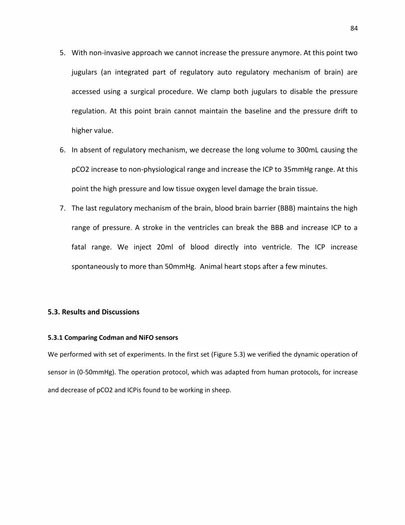
84
5. With non-invasive approach we cannot increase the pressure anymore. At this point two
jugulars (an integrated part of regulatory auto regulatory mechanism of brain) are
accessed using a surgical procedure. We clamp both jugulars to disable the pressure
regulation. At this point brain cannot maintain the baseline and the pressure drift to
higher value.
6. In absent of regulatory mechanism, we decrease the long volume to 300mL causing the
pCO2 increase to non-physiological range and increase the ICP to 35mmHg range. At this
point the high pressure and low tissue oxygen level damage the brain tissue.
7. The last regulatory mechanism of the brain, blood brain barrier (BBB) maintains the high
range of pressure. A stroke in the ventricles can break the BBB and increase ICP to a
fatal range. We inject 20ml of blood directly into ventricle. The ICP increase
spontaneously to more than 50mmHg. Animal heart stops after a few minutes.
5.3. Results and Discussions
5.3.1 Comparing Codman and NiFO sensors
We performed with set of experiments. In the first set (Figure 5.3) we verified the dynamic operation of
sensor in (0-50mmHg). The operation protocol, which was adapted from human protocols, for increase
and decrease of pCO2 and ICPis found to be working in sheep.
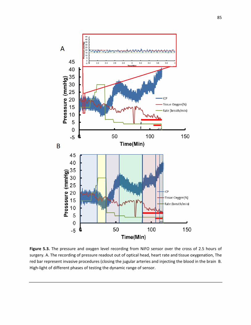
85
Figure 5.3. The pressure and oxygen level recording from NiFO sensor over the cross of 2.5 hours of
surgery. A. The recording of pressure readout out of optical head, heart rate and tissue oxygenation, The
red bar represent invasive procedures (closing the jugular arteries and injecting the blood in the brain B.
High-light of different phases of testing the dynamic range of sensor.

86
Figure 5.4. Ex-vivo monitoring of IOP. The KPro device with an embedded NiFO sensor is implanted. The
ocular pressure is increased using a syringe and measure directly using a digital manometer.
The acquisitions from all three sensors are shown in Figure 5.5 (the data is collected in different
time interval so the time access is not continues). We collect the signal to insure the sensor is not
damaged during implantation. In this phase, the ICP pressure is in the baseline line (16-18 mmHg) and
1minute signal is collected from each sensor to calculate the signal to noise ratio. All three sensors work
properly after implantation and the signal to noise ratio match the previous value collected in the lab
setting (Figure 5.6).

87
Figure 5.5. comparing average Codman microsensor and optical signal from three NiFO microsensors.
Time is in seconds. The sensors are recorded at discreet time intervals. The new acquisition is
highlighted using a blue arrow. The raw signal from each channel is also shown. The blue window
highlights the acquisition before closing the skin.

88
5.3.2 NiFO signal to noise ratio
The noise in the system is consisting of two distinct sources: 1. Optical noise due to quantum
fluctuation, scattering and 2: electrical noise from amplification. Both noises affect the reading but the
different approach is required to deal with each source of noise.
5.4. Conclusion
The aim of this chapter was to assess whether the novel microsensor can reliably record
pressure in vivo though the skin. The data obtained from 7 microsensors in 2 non-recovery
surgeries show the feasibility of optical reading with less than 2mmHg accuracy in the range of
0-50mmHg, the criteria which is sufficient to establish the NiFO monitoring consistency with
AAIM standard. The experience from this early implantations revealed some technical issues
associated with the sensor design, implantation method and ICP monitoring challenges.
In-vivo experiments have been conducted to optimize the surgical technique. In addition, we have
consulted with experienced animal users who have significant experience on minimizing pain and
distress. In the long-term experiments, all animals that receive ICP monitor implantation are expected to
have some post-operative discomfort which will be treated with analgesics, as described. All animals will
be euthanized at the conclusion of the experiment. Severe complications for all experiments include
anesthetic related deaths, cardiac dysrhythmias, intraocular hemorrhage, wound dehiscence, and
infection.
Anesthetic deaths can be limited by minimizing the duration of inhalational anesthesia. Cardiac
dysrhythmias can be minimized by monitoring arterial blood pressure and treated with internal
defibrillation. Intraocular hemorrhage can be minimized with the help of a surgical assistant to assemble
the corneal button to the KPro set, decreasing the time of open globe surgery, while the surgeon
performs the lens extraction. Infection will be prevented as best as possible by giving antibiotics,
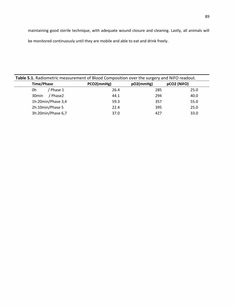
89
maintaining good sterile technique, with adequate wound closure and cleaning. Lastly, all animals will
be monitored continuously until they are mobile and able to eat and drink freely.
Table 5.1. Radiometric measurement of Blood Composition over the surgery and NiFO readout. Time/Phase PCO2(mmHg) pO2(mmHg) pCO2 (NiFO)
0h / Phase 1 26.4 285 25.0
30min / Phase2 44.1 294 40.0
1h:20min/Phase 3,4 59.3 357 55.0
2h:10min/Phase 5 22.4 395 25.0
3h:20min/Phase 6,7 37.0 427 33.0

90
CHAPTER 6
CONCLUSIONS AND FUTURE WORK
6.1. Conclusion
In this work we introduced two platforms to study the role of mechanical pressure in the axonal
injury response: 1. a microfluidic microchip as a platform for single cell level mechanical stress
studied in Drosophila larvae, and 2. a microsensor for continuous measurement of pressure in
mammalian models adapted into two examples: glaucoma and traumatic brain injury.
Our preliminary results show that the mechanical stress could slow down the axonal
transport and therefore play an important role in Wallerian degeneration. Our single cell results
also highlight the importance of pressure variation versus pressure level in neural injury. This
finding, if it will be verified in more complex model, could make a strong case for the use of the
continuous pressure monitoring platform we proposed in this work. On the other hand, we
showed the NiFO technology, even when it is used through a sheep skin, is sufficiently reliable
and accurate to satisfy the American medical instrument standard. The long-term implanation
capability of NiFO sensor open the way for continuous pressure monitoring in-vivo.

91
We envision that the signal cell study platform in this work can be used to improve the
understanding of the mechanism of axonal injury. Also our in-vivo pressure monitoring platform
may enhance the treatment planning in the future.
6.1.1. Single Cell Model to Study Neuronal Injury
We introduced an in-vivo neural injury model in Drosophila larvae to study the effect of chronic
pressure on the neural regeneration after injury. Using a microchip designed to immobilize and
image larvae, we studied the effect of pressure on the larvae motorneurons by simulating the
chronic pressure effect on a neuron. The on-chip studies show that the level of pressure and
the frequency of periodic mechanical stress both play a role in the injury initiation while the
role of the duration of high stress cycle is not significant. Base on this new finding, the
mechanical stress may slow down the axonal transport and consequently reduce the
regeneration speed in the damage neuron. This technique could be used to study the molecular
pathways modulating the axonal regeneration in response to environmental mechanical
stresses. Also, we envision this method could be used to demonstrate that the continuous
pressure monitoring could use to predict the axonal injury response in the long-term.
6.1.2. NiFO Technology to Study Injury Response to Mechanical Stress in the Mammalian
Animal Models
The implantable near infrared optical (NiFO) pressure sensor proposed in this work, was
adapted to measure intraocular and intracranial pressure:(i)we envision the NiFO technology to
be used to monitor the ocular pressure in glaucoma patients. By demonstrating a well-
established procedure for microsensor implantation in the human eye globe, we showed the
microsensor remain functional in an ex-vivo environment for at least 7 days. (ii) We envision the
92
NiFO technology could be used to monitor the cranial pressure in traumatic brain injury
patients. The microsensor had a small drift in an ex-vivo environment and was sufficiently
accurate to meet American medical associate standards for cranial pressure monitoring. This
platform could be used to demonstrate that the continuous pressure monitoring improves the
treatment planning for glaucoma and traumatic brain injury patients.
6.1.3. Monitor Pressure and Tissue Oxygenation in-vivo
We implanted the NiFO device in-vivo and demonstrated the device was functional in the
clinical setting. The readings from optical intracranial pressure sensor in the sheep model was
consistent with direct measurement form clinical goal standard monitoring device (Codman
Sensor). We also demonstrated that the dynamic response of the microsensor in in-vivo
environment. The sensor was able to track 1mmHg/second change in the ICP in the range of 0-
50mmHg. We envision in the next step the same implantation and measurement technique can
be used to establish whether the performance of the NiFO sensor deteriorates over time.
6.2. Future Works
6.2.1. Fabry-Perot Laser Cavity Pressure Sensor Technology In-vivo
. There are two main drawbacks to NiFO technology: 1. the resolution limitation due to light
diffraction limit. 2. The size of device cannot be reduced due to large deflection limitation.
These two drawbacks are particularly important in the case of IOP. To address this issue we
introduced a new technology based on the Fabry-Perot laser (FPL) cavity. In the next step we
will implant FPL microsensor are compare their performance to NiFO sensor. In addition to
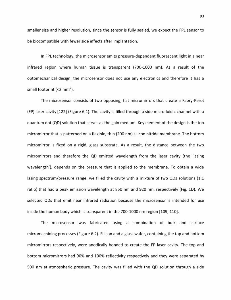
93
smaller size and higher resolution, since the sensor is fully sealed, we expect the FPL sensor to
be biocompatible with fewer side effects after implantation.
In FPL technology, the microsensor emits pressure-dependent fluorescent light in a near
infrared region where human tissue is transparent (700-1000 nm). As a result of the
optomechanical design, the microsensor does not use any electronics and therefore it has a
small footprint (<2 mm2).
The microsensor consists of two opposing, flat micromirrors that create a Fabry-Perot
(FP) laser cavity [122] (Figure 6.1). The cavity is filled through a side microfluidic channel with a
quantum dot (QD) solution that serves as the gain medium. Key element of the design is the top
micromirror that is patterned on a flexible, thin (200 nm) silicon nitride membrane. The bottom
micromirror is fixed on a rigid, glass substrate. As a result, the distance between the two
micromirrors and therefore the QD emitted wavelength from the laser cavity (the ‘lasing
wavelength’), depends on the pressure that is applied to the membrane. To obtain a wide
lasing spectrum/pressure range, we filled the cavity with a mixture of two QDs solutions (1:1
ratio) that had a peak emission wavelength at 850 nm and 920 nm, respectively (Fig. 1D). We
selected QDs that emit near infrared radiation because the microsensor is intended for use
inside the human body which is transparent in the 700-1000 nm region [109, 110].
The microsensor was fabricated using a combination of bulk and surface
micromachining processes (Figure 6.2). Silicon and a glass wafer, containing the top and bottom
micromirrors respectively, were anodically bonded to create the FP laser cavity. The top and
bottom micromirrors had 90% and 100% reflectivity respectively and they were separated by
500 nm at atmospheric pressure. The cavity was filled with the QD solution through a side
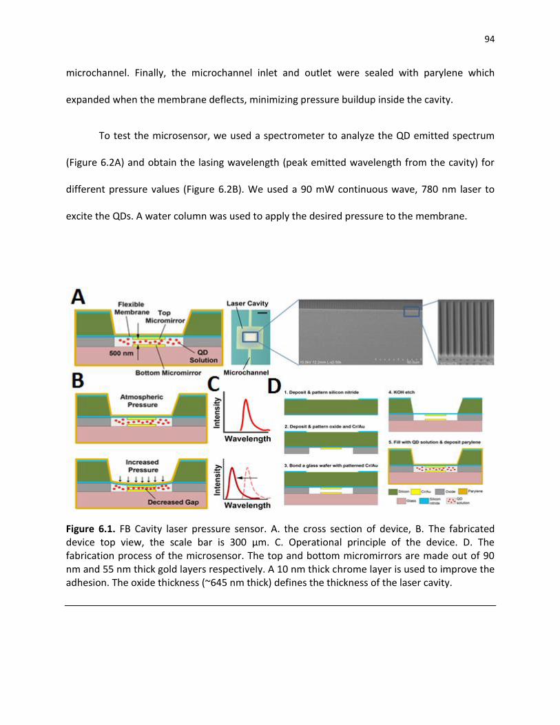
94
microchannel. Finally, the microchannel inlet and outlet were sealed with parylene which
expanded when the membrane deflects, minimizing pressure buildup inside the cavity.
To test the microsensor, we used a spectrometer to analyze the QD emitted spectrum
(Figure 6.2A) and obtain the lasing wavelength (peak emitted wavelength from the cavity) for
different pressure values (Figure 6.2B). We used a 90 mW continuous wave, 780 nm laser to
excite the QDs. A water column was used to apply the desired pressure to the membrane.
Figure 6.1. FB Cavity laser pressure sensor. A. the cross section of device, B. The fabricated device top view, the scale bar is 300 µm. C. Operational principle of the device. D. The fabrication process of the microsensor. The top and bottom micromirrors are made out of 90 nm and 55 nm thick gold layers respectively. A 10 nm thick chrome layer is used to improve the adhesion. The oxide thickness (~645 nm thick) defines the thickness of the laser cavity.

95
Figure 6.2. A. At 40 mmHg, the lasing wavelength of the microsensor is ~900 nm wavelength. B.
Lasing wavelength versus applied pressure.
6.2.2. Long-term Validate of the NiFO sensors In-vivo
We fabricated and demonstrated the functionality of NiFO sensor in-vivo. The next goal will be
to establish whether the performance of the NiFO sensor deteriorates over time (e.g. drift in
the ICP measurements). To do so, we will repeat the experiments described above every 2
weeks for a total duration of 2 months (we will obtain recordings the 12th, 14th, 16th and 18th
week). Animals will be fed normally during each 2-week period and will be anesthetized only for
the duration of the actual experiments (e.g. for 4-5 hours during the day of the ICP recording).
After the initial implantation (weeks 9-10), the Codman microsensor will be tunneled
through the scalp and attached to the adjacent scalp whereas the NiFO sensor will be
completely contained below the scalp. For the biweekly periodic readings, the Codman
microsensor will be reattached to the monitoring unit, and the optical reader will be used
through the scalp to obtain ICP readings.
At the conclusion of the data collection period (week 18th), each sheep will be
euthanized with pentobarbital, after which the brain will be removed, exposed to fixative, and

96
serially sectioned to be examined for gross pathological evidence of tissue damage resulting
from catheter placement.
After the collection of the ICP measurements from all sheep, we will perform correlation
analysis to find statistically significant ties and regression analysis to quantify the trends (e.g. t-
tests will be used to find significant differences between the recordings from the Codman and
NiFO sensors). At the end of monitoring period (week 18th), the NiFO sensors will be removed
from the sheep’s brain and they will be tested for zero drift in the laboratory. A range of
pressures of known magnitude will be applied to the devices and the corresponding signal will
be recorded. These results will be compared to the pressure-intensity graphs obtained for each
sensor before implantation.
6.2.3. Regulation path and biocompatibility
With an indication stated as “An intracranial pressure monitoring device is a device used for
short-term monitoring and recording of intracranial pressures” our proposed device would be
considered an Intracranial Pressure Measuring Device, as defined in Title 21 CFR 882.1620, and
would be considered a Class II medical device by the U.S. FDA (implantable ICP shunts for long-
term use are also Class II according to FDA). Thus, the regulatory pathway will require
submission of a Premarket Notification (510k) application to gain FDA approval to
commercialize the device in the U.S. We anticipate the FDA will require clinical trial data to
prove the safety and efficacy of the NiFO sensors. The clinical trial will be conducted under an
FDA and IRB approved Investigational Device Exemption (IDE) application. In order to gain the
FDA’s approval, we will need to design, develop and test the device following FDA Design

97
Control, Quality System Regulation (QSR), GLP, GMP and GCP requirements. We plan to engage
a regulatory affairs consultant to help us prepare a comprehensive regulatory strategy (CRS)
which will detail the bench, animal and clinical study validation testing and regulatory
requirements needed throughout the translational development life cycle of our device
development project.
98
Bibliography
[1] M. Devor, et al. Two modes of cutaneous reinnervation following peripheral nerve injury. The Journal of comparative neurology 185:1, 211-220, 2004.
[2] G. O. Lundborg, R. O. Myers, and H. E. N. R. Y. Powell. Nerve compression injury and increased endoneurial fluid pressure: a miniature compartment syndrome. Journal of Neurology, Neurosurgery & Psychiatry 46:12, 1119-1124, 1983.
[3] E. C. Johnson, et al. Global changes in optic nerve head gene expression after exposure to elevated intraocular pressure in a rat glaucoma model. Investigative ophthalmology & visual science 48:7, 3161-3177, 2007.
[4] D. Rempel, D. Lars, and G. Lundborg. Pathophysiology of Nerve Compression Syndromes: Response of Peripheral Nerves to Loading. The Journal of Bone & Joint Surgery 81:11, 1600-10, 1999.
[5] B. A. Yankner, Mechanisms of Neuronal Degeneration Review in Alzheimer’s Disease. Neuron 16, 921-932, 1996.
[6] A. L. McCormack, Alison L., et al. Environmental risk factors and Parkinson's disease: selective degeneration of nigral dopaminergic neurons caused by the herbicide paraquat. Neurobiology of disease 10:2, 119-127, 2002.
[7] E. Garcia‐Valenzulela, et al. Apoptosis in adult retinal ganglion cells after axotomy. Journal of neurobiology 25:4, 431-438, 1994.
[8] G. Stoll, Wallerian degeneration in the peripheral nervous system: participation of both Schwann cells and macrophages in myelin degradation. Journal of neurocytology 18:5, 671-683, 1989.
[9] M. Abercrombie, and M. L. Johnson. Quantitative histology of Wallerian degeneration: I. Nuclear population in rabbit sciatic nerve. Journal of anatomy 80:1, 37, 1946.
[10] C. Beaulieu, Changes in water diffusion due to Wallerian degeneration in peripheral nerve. Magnetic resonance in medicine 36:4, 627-631, 2005.
[11] C. Ikonomidou, and T. Lechoslaw, Neurodegenerative disorders: clues from glutamate and energy metabolism. Critical reviews in neurobiology 10:2, 239, 1996.
[12] T. Carlstedt, et al. Nerve fibre regeneration across the PNS-CNS interface at the root-spinal cord junction. Brain research bulletin 22.1, 93-102, 1989.
99
[13] R. George, and J. W. Griffin. The proximo-distal spread of axonal degeneration in the dorsal columns of the rat. Journal of neurocytology 23:11, 657-667, 1994.
[14] G. Stoll, S. Jander, and R. R. Myers. Degeneration and regeneration of the peripheral nervous system: from Augustus Waller's observations to neuroinflammation. Journal of the Peripheral Nervous System 7:1, 13-27, 2008.
[15] G. Stoll, and H. W. Müller. Nerve injury, axonal degeneration and neural regeneration: basic insights. Brain pathology 9:2, 313-325, 1999.
[16] C. Profyris, Degenerative and regenerative mechanisms governing spinal cord injury. Neurobiology of disease 15:3, 415-436, 2004.
[17] S. Hanz, et al. Axoplasmic importins enable retrograde injury signaling in lesioned nerve. Neuron 40:6, 1095-1104, 2003.
[18] H. W, Müller, and G. Stoll. Nerve injury and regeneration: basic insights and therapeutic interventions. Current opinion in neurology 11:5, 557-562, 1998.
[19] P. Yurco, and D.A. Cameron. Responses of Müller glia to retinal injury in adult zebrafish. Vision research 45:8, 991-1002, 2005.
[20] Y. Yajima, et al. Involvement of a spinal brain-derived neurotrophic factor/full-length TrkB pathway in the development of nerve injury-induced thermal hyperalgesia in mice. Brain research 958:2, 338, 2002.
[21] M. F. Yanik, Neurosurgery: Functional regeneration after laser axotomy. Nature 432, 822-822, 2004.
[22] M. Lee, Regeneration and functional reconnection of an identified vertebrate central neuron. The Journal of Neuroscience 2, 1793-1811, 1982.
[23] D. Ayaz, et al. Axonal Injury and Regeneration in the Adult Brain of Drosophila. The Journal of Neuroscience 28, 6010-6021, 2008.
[24] D. Kamber, H. Erez, and M. E. Spira, Local calcium-dependent mechanisms determine whether a cut axonal end assembles a retarded endbulb or competent growth cone. Experimental Neurology 219, 112-125, 2009.
[25] N. E. Ziv, and M.E. Spira, Localized and Transient Elevations of Intracellular Ca2+ Induce the Dedifferentiation of Axonal Segments into Growth Cones. The Journal of Neuroscience 17, 3568-3579, 1997.
[26] H. H. Liu, and S. T. Brady, cAMP, tubulin, axonal transport, and regeneration. Experimental Neurology 189, 199-203, 2004.
[27] S. Yoo, E.A. Niekerk, T. T. Merianda, and J. L. Twiss, Dynamics of axonal mRNA transport and implications for peripheral nerve regeneration. Experimental Neurology 223, 19-27, 2010.
[28] M.P. Coleman, and M.R. Freeman, Wallerian degeneration, wld(s, and nmnat. Annu Rev Neurosci. 33, 245-267, 2010.

100
[29] A. Vogel, and V. Venugopalan, Mechanisms of Pulsed Laser Ablation of Biological Tissues. Chemical Reviews 103, 577-644, 2003.
[30] S. X. Guo, et al. Femtosecond laser nanoaxotomy lab-on-a-chip for in vivo nerve regeneration studies. Nat Meth 5, 531-533, 2008.
[31] S. Chung, D. Clark, C. Gabel, E. Mazur, and A. Samuel, The role of the AFD neuron in C. elegans thermotaxis analyzed using femtosecond laser ablation. BMC Neuroscience 7, 30, 2006.
[32] Z. Wu, et al. Caenorhabditis elegans neuronal regeneration is influenced by life stage, ephrin signaling, and synaptic branching. Proceedings of the National Academy of Sciences 104, 15132-15137, 2007.
[33] M. Hammarlund, P. Nix, L. Hauth, E.M. Jorgensen, and M. Bastiani, Axon Regeneration Requires a Conserved MAP Kinase Pathway. Science 323, 802-806, 2009.
[34] T. V. Chokshi, A. Ben-Yakar, and N. Chronis, CO2 and compressive immobilization of C. elegans on-chip. Lab on a Chip 9, 151-157, 2009.
[35] K. Chung, and H. Lu, Automated high-throughput cell microsurgery on-chip. Lab on a Chip 9, 2764-2766, 2009.
[36] P. Fuger, L. B. Behrends, S. Mertel, S. J. Sigrist, and T. M. Rasse, Live imaging of synapse development and measuring protein dynamics using two-color fluorescence recovery after photo-bleaching at Drosophila synapses. Nat. Protocols 2, 3285-3298, 2007.
[37] M. R. Freeman, and J. Doherty, Glial cell biology in Drosophila and vertebrates. Trends in Neurosciences 29, 82-90, 2006.
[38] S. Banerjee, and M. Bhat, Glial ensheathment of peripheral axons in Drosophila. J Neurosci Res. 86, 1189-1198, 2008.
[39] X. Xiong, et al. Protein turnover of the Wallenda/DLK kinase regulates a retrograde response to axonal injury. The Journal of Cell Biology 191, 211-223, 2010.
[40] J. M. MacDonald, et al. The Drosophila Cell Corpse Engulfment Receptor Draper Mediates Glial Clearance of Severed Axons. Neuron 50, 869-881, 2006.
[41] E. D. Hoopfer, et al. Wlds Protection Distinguishes Axon Degeneration following Injury from Naturally Occurring Developmental Pruning. Neuron 50, 883-895, 2006.
[42] A. D. Pilling, D. Horiuchi, C. M. Lively, and W. M. Saxton, Kinesin-1 and Dynein Are the Primary Motors for Fast Transport of Mitochondria in Drosophila Motor Axons. Mol. Biol. Cell 17, 2057-2068 , 2006.
[43] S. Gunawardena, et al. Disruption of Axonal Transport by Loss of Huntingtin or Expression of Pathogenic PolyQ Proteins in Drosophila. Neuron 40, 25-40, 2003.
[44] K. E. Miller, et al. Direct Observation Demonstrates that Liprin-[alpha] Is Required for Trafficking of Synaptic Vesicles. Current Biology 15, 684-689, 2005.
101
[45] A. Schmid, et al. Activity-dependent site-specific changes of glutamate receptor composition in vivo. Nat Neurosci 11, 659-666, 2008.
[46] D. J. Sandstrom, Isoflurane depresses glutamate release by reducing neuronal excitability at the Drosophila neuromuscular junction. The Journal of Physiology 558, 489-502, 2004.
[47] D. J. Sandstrom, Isoflurane Reduces Excitability of Drosophila Larval Motoneurons by Activating a Hyperpolarizing Leak Conductance. Anesthesiology 108, 434-446 , 2008.
[48] M. A. Unger, H.P. Chou, T. Thorsen, A. Scherer, and S.R. Quake, Monolithic Microfabricated Valves and Pumps by Multilayer Soft Lithography. Science 288, 113-116, 2000.
[49] L. Tian, et al. Imaging neural activity in worms, flies and mice with improved GCaMP calcium indicators. Nat Meth 6, 875-881, 2009.
[50] M. C. Stone, M. M. Nguyen, J. Tao, D.L. Allender, and Rolls, M.M. Global Up-Regulation of Microtubule Dynamics and Polarity Reversal during Regeneration of an Axon from a Dendrite. Mol. Biol. Cell 21, 767-777, 2010.
[51] A. Ghosh-Roy, Z. Wu, A. Goncharov, Y. Jin, and A. D. Chisholm, Calcium and Cyclic AMP Promote Axonal Regeneration in Caenorhabditis elegans and Require DLK-1 Kinase. The Journal of Neuroscience 30, 3175-3183, 2010.
[52] J. Knöferle, et al. Mechanisms of acute axonal degeneration in the optic nerve in vivo. Proceedings of the National Academy of Sciences, 2010.
[53] J. A. Wolf, P. K. Stys, T. Lusardi, D. Meaney, and D. H. Smith, Traumatic Axonal Injury Induces Calcium Influx Modulated by Tetrodotoxin-Sensitive Sodium Channels. The Journal of Neuroscience 21, 1923-1930, 2001.
[54] J. M. Scholey, Kinesin-II, a membrane traffic motor in axons, axonemes, and spindles. The Journal of Cell Biology 133, 1-4, 1996.
[55] N. Hirokawa, and R. Takemura, Molecular motors and mechanisms of directional transport in neurons. Nat Rev Neurosci 6, 201-214, 2005.
[56] S. Rao, C. Lang, E. S. Levitan, and D. L. Deitcher, Visualization of neuropeptide expression, transport, and exocytosis in Drosophila melanogaster. Journal of Neurobiology 49, 159-172, 2001.
[57] K. A. Edwards, M. Demsky, R.A. Montague, N. Weymouth, and D.P. Kiehart, GFP-Moesin Illuminates Actin Cytoskeleton Dynamics in Living Tissue and Demonstrates Cell Shape Changes during Morphogenesis inDrosophila. Developmental Biology 191, 103-117 , 1997.
[58] T. Misgeld, M. Kerschensteiner, F. M. Bareyre, R. W. Burgess, and J.W. Lichtman, Imaging axonal transport of mitochondria in vivo. Nat Meth 4, 559-561, 2007.
[59] S. M. Martin, G.S. O'Brien, C. Portera-Cailliau, and A. Sagasti, Wallerian degeneration of zebrafish trigeminal axons in the skin is required for regeneration and developmental pruning. Development 137, 3985-3994, doi:10.1242/dev.053611, 2010.
[60] M. E. Vargas, and B. A. Barres, Why is Wallerian degeneration in the CNS so slow? Annu Rev Neurosci. 30, 153-179, 2007.

102
[61] J. A. Ainsley, et al. Enhanced Locomotion Caused by Loss of the Drosophila DEG/ENaC Protein Pickpocket1. Current Biology 13, 1557-1563, 2003.
[62] M. Fujioka, et al. Even-skipped, acting as a repressor, regulates axonal projections in Drosophila. Development 130, 5385-5400, 2003.
[63] J. Rietdorf and A. Steitz, E., Heidelberg. Linear unmixing macro for ImageJ, http://www.embl.de/eamnet/index.html, 2004.
[64] N. Aggarwal, and W. C. Karl, Line detection in images through regularized hough transform. Image Processing, IEEE Transactions on 15, 582-591, 2006.
[65] X. Chenyang, and J. L. Prince, Snakes, shapes, and gradient vector flow. Image Processing, IEEE Transactions on 7, 359-369, 1998.
[66] Z. Shan, and M. Kai-Kuang, A new diamond search algorithm for fast block-matching motion estimation. Image Processing, IEEE Transactions on 9, 287-290, 2000.
[67] T. Lee, and L. Luo, Mosaic Analysis with a Repressible Cell Marker for Studies of Gene Function in Neuronal Morphogenesis. Neuron 22, 451-461, 1999.
[68] D. Dutta, J.W. Bloor, M. Ruiz-Gomez, K. VijayRaghavan, and D.P. Kiehart, Real-time imaging of morphogenetic movements in drosophila using Gal4-UAS-driven expression of GFP fused to the actin-binding domain of moesin. Genesis 34, 146-151, 2002.
[69] J. A. Fischer, et al. GAL4 activates transcription in Drosophila. Nature 853-856, 1998.
[70] J. B. Duffy, GAL4 system in Drosophila: a fly geneticist's Swiss army knife. Genesis 34.1‐2, 1-15, 2002.
[71] R. Ravi and R. J. Morgan, Intracranial pressure monitoring, Current Anaesthesia & Critical Care, vol. 14, pp. 229-235, 2003.
[72] A. Marmarou, et al., Impact of ICP instability and hypotension on outcome in patients with severe head trauma, Special Supplements, vol. 75, pp. S59-S66, 1991.
[73] J. E. Huizenga, et al., Guidelines for the Management of Severe Head Injury: Are Emergency Physicians Following Them?, Academic Emergency Medicine, vol. 9, pp. 806-812, 2002.
[74] M. Czosnyka and J. D. Pickard, Monitoring and interpretation of intracranial pressure, Journal of Neurology, Neurosurgery & Psychiatry, vol. 75, pp. 813-821, June 1, 2004 2004.
[75] T. G. Saul and T. B. Ducker, Effect of intracranial pressure monitoring and aggressive treatment on mortality in severe head injury, Journal of Neurosurgery, vol. 56, pp. 498-503, 1982.
[76] G. L. Clifton, et al., Fluid thresholds and outcome from severe brain injury*, Critical Care Medicine, vol. 30, pp. 739-745, 2002.
[77] J. Zhong, et al., Advances in ICP monitoring techniques, Neurological Research, vol. 25, pp. 339-350, 2003.
103
[78] M. H. Morgalla, ICP measurement accuracy: the effect of temperature drift. Design of a laboratory test for assessment of ICP transducers, Journal of medical engineering & technology, vol. 23, p. 10, 1999.
[79] C. Sander, et al., A monolithic capacitive pressure sensor with pulse-period output, in Solid-State Circuits Conference. Digest of Technical Papers. 1980 IEEE International, 1980, pp. 78-79.
[80] K. Wen Hsiung, et al., Development of a miniature pressure transducer for biomedical applications, Electron Devices, IEEE Transactions on, vol. 26, pp. 1896-1905, 1979.
[81] R. Magjarevic, et al., Design of a Wireless Intraocular Pressure Monitoring System for a Glaucoma Drainage Implant, in 13th International Conference on Biomedical Engineering. vol. 23, C. T. Lim and J. C. H. Goh, Eds., ed: Springer Berlin Heidelberg, 2009, pp. 198-201.
[82] K. C. Katuri, et al., A surface micromachined capacitive pressure sensor for intraocular pressure measurement, in Mechatronics and Embedded Systems and Applications, MESA, 2010 IEEE/ASME International Conference on, 2010, pp. 149-154.
[83] M. Gelabert-González, et al., The Camino intracranial pressure device in clinical practice. Assessment in a 1000 cases, Acta Neurochirurgica, vol. 148, pp. 43[5-441, 2006.
[84] J. Dings, et al., Clinical Experience with 118 Brain Tissue Oxygen Partial Pressure Catheter Probes, Neurosurgery, vol. 43, pp. 1082-1094, 1998.
[85] L.-O. D. Koskinen and M. Olivecrona, Clinical Experience with the Intraparenchymal Intracranial Pressure Monitoring Codman MicroSensor System, Neurosurgery, vol. 56, pp. 693-698, 2005.
[86] M. Jensen, et al., Risk factors of intracranial pressure monitoring in children with fiberoptic devices : A critical review. Commentary, Surgical Neurology, vol. 47, pp. 16-22, 1997.
[87] J. S. Kroin, et al., Long-term testing of an intracranial pressure monitoring device, Journal of Neurosurgery, vol. 93, pp. 852-858, 2000.
[88] U. Kawoos, et al., A permanently implantable intracranial pressure monitor, in Bioengineering Conference, 2005. Proceedings of the IEEE 31st Annual Northeast, 2005, pp. 17-19.
[89] N. Najafi and A. Ludomirsky, Initial Animal Studies of a Wireless, Batteryless, MEMS Implant for Cardiovascular Applications, Biomedical Microdevices, vol. 6, pp. 61-65, 2004.
[90] CardioMEMS. Available: http://www.cardiomems.com/
[91] U. Kawoos, et al., In-Vitro and In-Vivo Trans-Scalp Evaluation of an Intracranial Pressure Implant at 2.4 GHz, Microwave Theory and Techniques, IEEE Transactions on, vol. 56, pp. 2356-2365, 2008.
[92] M. A. Poca, et al., Is intracranial pressure monitoring in the epidural space reliable? Fact and fiction, Journal of Neurosurgery, vol. 106, pp. 548-556, 2007.
[93] L. Hardell, et al., Tumour risk associated with use of cellular telephones or cordless desktop telephones, World Journal of Surgical Oncology, vol. 4, p. 74, 2006.
[94] V. Ntziachristos, et al., Looking and listening to light: the evolution of whole-body photonic imaging, Nat Biotech, vol. 23, pp. 313-320, 2005.

104
[95] L. T. Rosenblum, et al., Optimizing quantitative in vivo fluorescence imaging with near-infrared quantum dots, Contrast Media & Molecular Imaging, pp. 120-129, 2010.
[96] W. Hu, et al., Three-dimensional SU-8 structures by reversal UV imprint, Journal of Vacuum Science & Technology B: Microelectronics and Nanometer Structures, vol. 24, pp. 2225-2229, 2006.
[97] S. Coe-Sullivan, et al., Large-Area Ordered Quantum-Dot Monolayers via Phase Separation During Spin-Casting, Advanced Functional Materials, vol. 15, pp. 1117-1124, 2005.
[98] D. Maier-Schneider, et al., A new analytical solution for the load-deflection of square membranes, Microelectromechanical Systems, Journal of, vol. 4, pp. 238-241, 1995.
[99] E. Pehlke, et al., Shape and stability of quantum dots, Applied Physics A: Materials Science & Processing, vol. 65, pp. 52[5-534, 1997.
[100] O. V. Salata, et al., Uniform GaAs quantum dots in a polymer matrix, Applied Physics Letters, vol. 65, pp. 189-191, 1994.
[101] D. Qi, et al., Efficient polymer-nanocrystal quantum-dot photodetectors, Applied Physics Letters, vol. 86, pp. 093103-093103-3, 2005.
[102] X. Gao, et al., In vivo cancer targeting and imaging with semiconductor quantum dots, Nat Biotech, vol. 22, pp. 969-976, 2004.
[103] F. Martelli, et al., Light Propagation through Biological Tissue and Other Diffusive Media: SPIE Press, 2010.
[104] C. R. Simpson and et al., Near-infrared optical properties of ex vivo human skin and subcutaneous tissues measured using the Monte Carlo inversion technique, Physics in Medicine and Biology, vol. 43, p. 2465, 1998.
[105] A. N. Bashkatov and et al., Optical properties of human skin, subcutaneous and mucous tissues in the wavelength range from 400 to 2000 nm, Journal of Physics D: Applied Physics, vol. 38, p. 2543, 2005.
[106] W. J. O'Dowd, Medical Device Safety: The Regulation of Medical Devices for Public Health and Safety, Physics in Medicine and Biology, vol. 47, p. 349, 2002.
[107] S. Cova, et al., Avalanche photodiodes and quenching circuits for single-photon detection, Appl. Opt., vol. 35, pp. 1956-1976, 1996.
[108] R. R. Anderson, and J.A. Parrish. The optics of human skin. Journal of Investigative Dermatology 77.1, 13-19, 1981.
[109] T. L. Troy, and S. N. Thennadil. Optical properties of human skin in the near infrared wavelength range of 1000 to 2200 nm. Journal of Biomedical Optics 6.2, 167-176, 2001.
[110] C. R. Simpson, et al. Near-infrared optical properties of ex vivo human skin and subcutaneous tissues measured using the Monte Carlo inversion technique. Physics in Medicine and Biology 43:9. 2465, 1999.

105
[111] H. A. Quigley, E. M. Addicks, and W. R. Green. Optic nerve damage in human glaucoma. III. Quantitative correlation of nerve fiber loss and visual field defect in glaucoma, ischemic neuropathy, papilledema, and toxic neuropathy. Archives of ophthalmology 100:1, 135, 1981.
[112] J. Y. Li, M. A. Greiner, J. D. Brandt, M. C. Lim, and M. J. Mannis, Long-term Complications Associated with Glaucoma Drainage Devices and Boston Keratoprosthesis. Am J Ophthalmol. 152:209-218, 2011. [113] H. F. Chew, B. D. Ayres, K. M. Hammersmith, et al., Boston Keratoprosthesis Outcomes and Complications. Cornea.28:989-996, 2009. [114] P. A. Netland, H. Teruda, and C. H. Dohlman Glaucoma Associated with Keratoprosthesis. Ophthalmology.105:751-757, 1998. [115] R. Kamyar, J. S. Weizer, and F.H. Paula, Glaucoma Associated With Boston Type I Keratoprosthesis. Cornea. 31:134-139, 2012. [116] A. Krug, S. Kompa, and N. F. Schrage, The Aachen-Keratoprosthesis - a flexible KPro that permits intraocular pressure measurement. Int J Artif Organs. 25: 238-42, 2002. [117] P. A. Netland, H. Terada, and C. H. Dohlman, Glaucoma associated with keratoprosthesis. Ophthalmology. 105: 751-7, 1998. [118] M. Banitt, Evaluation and management of glaucoma after keratoprosthesis. Curr Opin Ophthalmol. 22:133-136, 2011. [119] A. Todani, I. Behlau, and M. A. Fava, Intraocular Pressure Measurement by Radio Wave Telemetry. Invest Ophthalmol Vis Sci. 52:9573-9580, 2011. [120] N. R. Kim, C. Y. Kim, H. Kim, G. J. Seong, and E. S. Lee, Comparison of Goldmann Applanation Tonometer, Noncontact Tonometer, and TonoPen XL for Intraocular Pressure Measurement in Different Types of Glaucomatous, Ocular Hypertensive, and Normal Eyes. Curr Eye Res. 3644, 2295-300, 2011. [121] T. M. AlMubrad and K. C. Ogbuehi, The effect of repeated applanation on subsequent IOP measurements. Clin Exp Optom, 91: 6: 524-529, 2008.
[122] C. H. Dohlman, J. C. Abad, E. J. Dudenhoefer, et al., Keratoprosthesis: beyond corneal graft failure. In: Spaeth, G.L., ed. Ophthalmic Surgery: Principles and Practice. 3rd ed. Philadelphia, PA: W. B. Saunders, 199-207, 2002.