ndt
DESCRIPTION
mptTRANSCRIPT

Durham E-Theses
Investigation into the use of zero angle ultrasonic probe
array for defect detection and location
Snowdon, Paul C.
How to cite:
Snowdon, Paul C. (2007) Investigation into the use of zero angle ultrasonic probe array for defect detection
and location, Durham theses, Durham University. Available at Durham E-Theses Online:http://etheses.dur.ac.uk/2283/
Use policy
The full-text may be used and/or reproduced, and given to third parties in any format or medium, without prior permission orcharge, for personal research or study, educational, or not-for-pro�t purposes provided that:
• a full bibliographic reference is made to the original source
• a link is made to the metadata record in Durham E-Theses
• the full-text is not changed in any way
The full-text must not be sold in any format or medium without the formal permission of the copyright holders.
Please consult the full Durham E-Theses policy for further details.

Academic Support O�ce, Durham University, University O�ce, Old Elvet, Durham DH1 3HPe-mail: [email protected] Tel: +44 0191 334 6107
http://etheses.dur.ac.uk
2

Preface
Copyright© 2007 by Paul C . Snowdon
The copyright of this thesis rests wi th the author. N o quotation f r o m i t should be
published without prior written consent and information derived f r o m it should be
acknowledged.
The copyright of this thesis rests with the author or the university to which it was submitted. No quotation from it, or information derived from it may be published without the prior written consent of the author or university, and any information derived from it should be acknowledged.
1 0 MAR 2008 i i

Preface
Acknowledgements
I would like to thank Dr . Sherri Johnstone o f the University o f Durham for her
supervision and support during my studies, and Professor David Wood and Professor
Mike Petty for their continuous encouragements.
I would also like to thank Dr . Stephen Dewey o f Corus Pic. for his support, and Corus
Pic. for their financial contribution to the project.
i i i
Preface
Abstract
The steel industry like any other manufacturing process is under constant pressure to
deliver higher quality defect free material at lower cost to customers. This push for
zero defects has led to improved manufacturing processes and the need for more
reliable, faster defect testing methods. Ultrasound fundamentally provides a mechanical
stress, produced by tensile, compressive, shearing or flexural forces, which are o f such
low intensity that no material damage occurs.
The remit o f the project was to investigate and develop the latent potential wi thin the
present automated ultrasonic immersion system using an array o f normal angle probes,
used for billet inspection. The work presented in this thesis describes the research
undertaken to develop a system using, 10mm diameter, standard zero angled 5MHz
ultrasonic transducers. The transducers were used at linear separation distances o f
between 22.5mm and 45mm set in a typical 8-probe array orientation.
The developed technique is potentially transferable to other ultrasonic multi-probe
array applications and demonstrates that time o f flight diffraction can be realised using
normal probes, and termed Normal Probe Dif f rac t ion , (NPD). The technique located
defects, using the intersection o f ellipses, wi th an error o f <0.5% o f the signal transit
distance and, wi th the application o f a correlation filter, improved the Signal to Noise
Ratio (SNR) f r o m - 2 . 0 d B to 17.0dB.
iv

Preface
Contents
Chapter 1. Motivation for the Project
1.1. Introduction 1-1
1.2. References 1-2
Chapter 2. Project Definition
2.1. Introduction 2-1
2.2. The Bloom and Billet M i l l 2-1
2.3. Automated Ultrasonic Test System 2-2
2.4. System Operation 2-4
2.5. Project Motivation 2-5
2.6. Conclusion 2-6
2.7. References 2-7
Chapter 3. Review of current systems and technologies
3.1. Introduction 3-1
3.2. Ultrasonic Methods 3-2
3.2.1. Generating Ultrasound 3-2
3.2.2. Piezoelectric Transducers 3-3
3.2.3. Electromagnetic Acoustic Transducers (EMAT) 3-6
3.2.4. Laser Generated Ultrasound 3-8
3.2.5. Inspection Techniques 3-9

Preface
3.2.6. Pulse/Echo 3-10
3.2.7. Through Transmission 3-13
3.2.8. Phased Array 3-14
3.2.9. Time of Flight Dif f rac t ion (ToFD) 3-15
3.2.10. Synthetic Aperture Focusing Technique (SAFT) 3-20
3.3. Visual and Optical Testing (VT) 3-22
3.4. Radiography Testing (RT) 3-23
3.5. Magnetic Particle Inspection (MPI) 3-25
3.6. Eddy Current Testing (EC) 3-27
3.7. Dye Penetrant Inspection (DVT) 3-29
3.8. Conclusion 3-31
3.9. References 3-33
Chapter 4. Review of Basic Theory
4.1. Introduction 4-1
4.2. Propagation and Velocity 4-1
4.3. Wave Propagation at Boundaries 4-5
4.4. Loss mechanisms 4-8
4.5. Dif f rac t ion o f Waves 4-11
4.6. Sound Pressure and Beam Profile 4-12
4.6.1. The Near and Far fields 4-13
4.6.2. Beam Profile 4-15
4.7. Signal to Noise Ratio 4-16
4.8. Inspection Dead Zone 4-17
4.9. Summary 4-18
4.10. References 4-19
v i

Preface
Chapter 5. System and Initial Experimental Work
5.1. Introduction 5-1
5.2. Experimental Apparatus 5-2
5.2.1. Hewlett Packard " I n f i n i u m " Oscilloscope 5-3
5.2.2. Socomate USPC 3100 5-4
5.2.3. Transducers 5-4
5.2.4. Transducer/Sample Coupling 5-6
5.3. Characterisation o f the System 5-8
5.3.1. Transmitter Voltage 5-9
5.3.2. Receiver Characteristics 5-10
5.4. Initial experiments to assess the use o f a single transmitter
multi-receiver system 5-12
5.4.1. Characterisation o f Billet 5-12
5.4.2. Experiment to assess the use o f passive receiver probes
5-14
5.5. Further experiments to assess the use o f passive receiver probes
5-19
5.5.1. Calibrated Sample 5-19
5.5.2. Pulse/Echo Scans 5-20
5.6. Multi-Probe Scan 5-26
5.6.1. Spurious Echo Investigation 5-31
5.7. Conclusion 5-39
5.8. References 5-42
vi i
Preface
Chapter 6. T i m e Ellipse Defect Location
6.1. Introduction 6-1
6.2. Ellipse Equations 6-2
6.3. Ellipse Calculations 6-3
6.4. Conclusion 6-6
6.5. References 6-7
Chapter 7. Signal E c h o Enhancement using D S P
7.1. Introduction 7-1
7.2. Digital Signal Processing 7-2
7.3. Cross-correlation Filtering 7-4
7.4. Pass-band Filtering 7-7
7.5. Filtering a Weak Signal 7-10
7.6. Cross-correlation Filtering o f a Weak Echo Signal 7-10
7.7. Pass-band Filtering o f a Weak Echo Signal 7-11
7.8. Combining the Techniques 7-12
7.9. Conclusion 7-15
7.10. References 7-16
Chapter 8. Multi-Probe Scan
8.1. Introduction 8-1
8.2. Detection Limits 8-2
8.3. Scanning the V I block 8-4
8.4. Filtering the B-scan 8-7
8.5. The N P D System 8-10
8.6. Conclusion 8-11
8.7. References 8-14
vi i i

Preface
Chapter 9. N P D Applied to a Section of Steel Billet
9.1. Introduction 9-1
9.2. General Experimental Set-Up 9-2
9.3. Immersion Inspection o f a 2.5mm Flat-bottomed Hole 9-3
9.4. B-scan o f the Flat-bottomed Hole 9-4
9.5. N P D Applied to a Naturally Occurring Discontinuity 9-6
9.6. Conclusion 9-9
9.7. References 9-11
Chapter 10. Conclusions and further work 10-1
10.1. References 10-6
Appendices
Contents including list o f publications 1
B-scans f r o m experimental work conducted in Chapter 9. 2
Publications 4
ix

Preface
Nomenclature
Symbol Quantity Units
a Attenuation coefficient N / / A
D Diameter o f a flat circular oscillator m
X Wavelength m
N Length o f near zone m
/ Frequency Hz
c Acoustic velocity m/s
Y Hal f angle o f divergence N / / A
V Particle velocity m/s
p Density k g / m 3
p Sound pressure Pa
Poisson's ratio N / / A
E Young's modulus GPa
G Modulus o f shear N / m 2
Z Acoustic impedance N s / m 3
P Acoustic power W
X

Motivation for the Project
Chapter 1„
Motivation for the Project
1.1. Introduction
The steel industry like any other manufacturing company is under constant pressure to
deliver higher quality "defect free" material at lower cost to customers. Improvements
in manufacturing processes and the use o f more sophisticated measurement systems
have seen a significant reduction in the number o f defective products wi th the aim o f
reaching the elusive goal o f zero failures [1]. This push for zero defects has lead to
improved manufacturing processes and the need for more reliable, faster defect testing
methods.
The standard ultrasonic technique for defect detection is the pulse/echo method, using
an array o f relatively low cost ultrasonic transducers. To improve on this method the
steel industry is tending to move towards complex phased array technologies. These
ultrasonic systems are relatively expensive and complex when compared to a basic
pulse/echo system. They also have a propensity o f being application specific, in that
the probes or probe-coupling shoe wi l l be tailored to a specific examination or
component location.
1-1

Motivation for the Project
The remit o f this project was to investigate the latent potential wi th in an existing
ultrasonic defect detection system installed at Thrybergh billet mi l l , Corus pic. This
system consists o f an array o f probes in which each probe sequentially fires and
receives an ultrasonic pulse as a steel billet travels past. The specific research question
to be addressed in this thesis is, i f the system is reconfigured such that after each probe
fires, all the probes are used to detect reflected pulses, can extra information about the
presence, size and type o f defects be improved?
Chapter 2 gives a description o f the manufacturing process at Thrybergh billet mi l l
together wi th the current ultrasonic defect detection system to be investigated. To put
the project into context, a literature review o f current technologies is presented in
Chapter 3 followed by the wave propagation theory required to understand the
technology researched in this project. T o study the system, an experimental rig was set
up in controlled laboratory conditions. This is described in Chapter 5 together with the
results f rom initial experimental work. Chapters 6 and 7 describe the experimental data
and analysis undertaken using the experimental rig to analyse the detected signals and
improve the signal the noise ratio. Finally, the work is critically assessed in Chapters 8
and 9 and summarised in Chapter 10.
1.2. References
1. Wolfram, A. Automated ultrasonic inspection, in 15th WCNDT conference. 2000. Rome, Italy, www.ndt.net/art icle/wcndt00/papers/idnl97/idnl97.htm
1-2
Project Defini t ion
Chapter 2.
Project Definition
2.1. Introduction
This chapter firstly describes the manufacturing process at Thrybergh billet mi l l such
that the purpose, operation and limitations o f the existing defect detection system can
be explained. The detailed project motivation wi l l then be presented in context wi th
this manufacturing process.
2.2. The Bloom and Billet Mill
The Bloom and Billet M i l l consists o f two distinct processes: the Primary M i l l and the
Finishing mil l . A t the Primary M i l l the molten steel is continuously cast as a 400 m m
square bloom. Dur ing the casting process, refractory shrouds cover the vessel to
prevent atmospheric exposure, which is the main cause o f inclusions being formed in
the molten steel [1 , 2, 3]. Oxides and sulphides are the most common inclusions found
in steel; these can be quite simple in nature containing just one component (e.g.
Alumina particles A1 2 0 3 ) but very often come as a much more complex, multi-
component construction, containing more than one inclusion.
2-1

Project Defini t ion
The solidified steel is then re-heated and rolled into a 180 m m square billet. I n addition
to the chemical variations, inclusions also vary in their size and shape [4], however the
hot rolling process elongates and concentrates these inclusions to the core o f the billet.
A n initial eddy current inspection o f the material (for surface breaking cracks) is done
at this stage prior to the steel leaving the mi l l . The steel is then transferred in billet
f o r m to the Finishing M i l l . A t the Finishing M i l l i t is reheated to 1200°C and rolled
down to the final size required of between 30-75mm. This process o f working the steel
also improves the quality o f the steel by refining its crystalline structure and making the
metal stronger and tougher. A n ultrasonic inspection process takes place after the
material has been hot rolled down to the final 30-75mm sizes and the evaluation o f the
ultrasonic signals is carried out wi th multi-channel electronics [5]. This is because the
coarse grain structure o f the as-cast bloom causes high attenuation o f ultrasound [6].
Thus, it is more practical to inspect the steel post hot rolling.
2.3. Automated Ultrasonic Test System
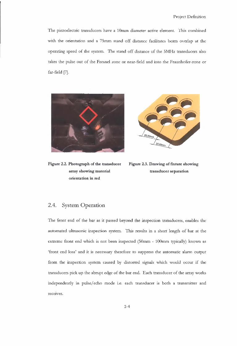
The current system is a stationary multi-transducer array, consisting o f two identical
banks o f immersion transducers set overlapping so that no part o f the material is left
un-inspected. These are arranged at normal incidence to the material and at 90° to each
other, as shown in Figure 2.2. This is used for the inspection o f square section, steel
billets ranging in size between 40mm to 80mm. The steel billet in this particular
inspection system is passed by the transducer arrays on the diamond as shown in red in
Figure 2.2. Each bank o f eight transducers is arranged as in Figure 2.3, the transducers
were activated sequentially, testing the steel using pulse/echo procedures.
2-2

Project Defini t ion
180 m m square billets arrive f r o m the Primary steel mil l
f
Steel re-heated to 1200°C 21 Stand H o t Rolling M i l l Steel re-heated to 1200°C 21 Stand H o t Rolling M i l l
Billets bundled &
penned
Shot-blaster
Ultrasonic Inspection
Cooling beds.
Material leaves < 50°C
Marking
2 stage Ultra-Violet Magnetic
Particle Inspection (MPT)
Accept
Despatch to
customer
Bundler
/ 1 1 \
Reject/Accept switch
Return to the accept
path, i f rectified
Reject
Rejec
t ,
t queue
/ 3 : X
Rectification &
Re-inspection
Figure 2.1. Schematic of the Bar M i l l f inishing line
2-3
Project Definition
The piezoelectric transducers have a 10mm diameter active element. This combined with the orientation and a 75mm stand of f distance facilitates beam overlap at the operating speed of the system. The stand off distance of the 5MHz transducers also takes the pulse out of the Fresnel zone or near-field and into the Fraunhofer-zone or far-field [7].
Figure 2.2. Photograph of the transducer Figure 2.3. Drawing of fixture showing
array showing material transducer separation
orientation in red
2.4. System Operation
The front end of the bar as it passed beyond the inspection transducers, enables the
automated ultrasonic inspection system. This results in a short length of bar at the
extreme front end which is not been inspected (50mm - 100mm typically) known as
'front end loss' and it is necessary therefore to suppress the automatic alarm output
from the inspection system caused by distorted signals which would occur i f the
transducers pick up the abrupt edge of the bar end. Each transducer of the array works
independendy in pulse/echo mode i.e. each transducer is both a transmitter and
receiver.
2-4

Project Defini t ion
The transducers are held at a distance o f approximately 70mm f r o m the material. This is both to alleviate the possibility that they wi l l be struck by the f ront end o f the moving bar, and to remove the complications involved wi th the near field o f the transducers. A n automated marking system, marks all defect affected areas that are encountered by the inspection system.
The pulse repetition frequency (PRF) o f the probe array is optimised to allow for signal
decay [8], and to give fu l l coverage o f the billet to be inspected, whilst operating at its
recommended throughput rate. Test throughput speeds are limited, not by the pulse
repetition rate, but by air entrapment and turbulence. The system is capable o f material
throughput speeds o f 2m/s, however at Thrybergh bar mi l l i t runs between 0.8m/s to
l m / s . The inspection is terminated prior to the tail end o f the bar passing over the
inspection transducers and again suppressing the alarm output similar to the front end.
This results in an additional un-inspected region at the tail end o f the bar, known as
'back end loss'. Bars, for which the line control logic has been alerted to the defective
nature o f the product, are tracked through the line and subsequently sorted into good
or defective groups. The defective bars are then manually re-inspected to qualify and
define the nature o f the defect.
2.5. Project Motivation
As the demand fo r cleaner steels increases every year [9] i t would be desirable f r o m
both an economic and environmental position to eliminate the primary re-heating and
rolling process altogether.
2-5

Project Defini t ion
This would have substantial influence on costs in energy expenditure and material handling. However this would place greater demands on the downstream N D T , as the intermediate N D T stage would also have been eliminated.
The remit o f the project is to investigate the core section o f the material using
ultrasonic techniques. The steel sections o f interest are square section billets wi th
dimensions ranging f r o m 76mm x 76mm down to 36mm x 36mm. The initial concept
was to use the Sonomat ic™ system as i t currently operates, but processing the received
transmission using several o f the probes. That is a single transmitter wi th multiple
receivers. The initial concept was deemed worthy o f further investigation because o f
the divergence o f the ultrasonic wave as i t is transmitted. When an ultrasonic probe is
fired, the pulse o f ultrasound is transmitted through the water coupling into the steel
billet, and is reflected o f f the back wall o f the steel (pulse/echo). As an ultrasonic beam
travels through a medium, i t diverges. When the signal is received back at the probe,
because o f the distance the signal has travelled, (in this case about 300mm), the
returning echo is over 4 times the diameter o f the original probe. There is therefore
potentially a substantial amount o f information not being collected by the single probe.
2.6. Conclusion
This chapter explains the reasoning behind this project in context to the operation o f
the Bloom and Billet M i l l process at Thrybergh M i l l and the limitations o f the existing
non-destructive testing technology currently utilised.
2-6
Project Defini t ion
2.7. References
1. Zhang, L . and B.G. Thomas. Inclusions in Continuous Casting of Steel, in XXIV NationalSteelmaking Symposium. 2003. Morelia, Mexico, p. 138-183
2. Kiessling, R., Non-metallic inclusions in steel. 1989, London: The Institute o f Metals.
3. Dekkers, R., Non-metallic inclusions in liquid steel. 2002, PhD. Thesis. Leuven Universiteit:
4. Singh, B. and S.K. Kaushik, Influence of steel-making processes on the quality of reinforcement. The Indian Concrete Journal, 2002. 76(7): p. 407-412.
5. Wolfram, A . Automated ultrasonic inspection, in / i * * WCNDT conference. 2000. Rome, Italy, www.ndt.net/art icle/wcndt00/papers/idnl97/idnl97.htm
6. Shin, B.-C. and J.-R. K w o n , Ultrasonic transducersfor continuous-cast billets. Sensors and Actuators A : Physical, 1996. 51: p. 173-177.
7. Krautkramer, J. and H . Krautkramer, Ultrasonic Testing of Materials. 4th ed. 1990, Berlin, Heidelberg, N e w York.: Springer-Verlag. p. 677.
8. Webb, P. and C. Wykes, Suppression of second-time-around echoes in high firing rate ultrasonic transducers. N D T & E International, 1995. 28(2): p. 89-93.
9. Zhang, L . , et al. Evaluation and Control of Steel Cleanliness - Review, in 85th
Steelmaking Conference Proceeding. 2002. Warrendale, PA, U.S.A. p. 431-452.
2-7

Review o f Current Systems and Technologies
Chapter 3.
Review of Current Systems and
Technologies
3.1. Introduction
This chapter gives an outline o f the major methods o f Non-Destructive Testing
( N D T ) , technologies currently employed for industrial inspection, such that the method
under investigation in this thesis can be compared to other methods. Since this method
is a variant o f two current ultrasonic techniques, the chapter starts by describing the
constraints within which ultrasonic testing is o f use. Different ultrasonic generating
transducers are then presented detailing their advantages and disadvantages. Describing
and comparing the different excitation configuration, analysis techniques and data
representations commonly used in commercial systems complete the ultrasonic testing
section.
The next part o f the chapter outlines and assesses other competing technologies such
as visual, radiography and magnetic particle inspection, and dye penetration. Finally,
the project remit is put into context wi th respect to the technologies presented in this
chapter.
3-1

Review o f Current Systems and Technologies
3.2. Ultrasonic Methods
Ultrasonic testing o f material properties is a commonly utilised technology that is
readily available commercially. Systems range f r o m basic pulse/echo systems to
scanning phased array systems employing digital signal processing to improve signal to
noise ratios and provide real-time data analysis. A typical ultrasonic system consists o f
a transducing system to transmit and receive ultrasonic waves, a coupling system to the
sample under inspection, a sample and finally analysis software. The type o f transducer
required depends on factors such as the frequency o f operation, the ambient
conditions, the method o f inspection, the mode o f propagation and cost and
availability. This section outlines both the different transducing and inspection
methods currendy available and contrasts and compares their performances.
3.2.1. Generating Ultrasound
The methods discussed in this section involve converting an electrical signal either
directly or indirectly into an ultrasonic wave, which propagates through a material.
They are:
• Piezoelectric transducers
• Electromagnetic Acoustic Transducers (EMAT)
• Laser Generated Ultrasound
3-2

Review o f Current Systems and Technologies
3.2.2. Piezoelectric Transducers
A transducer containing a piezoelectric element wi l l convert electrical signals into
mechanical vibrations in transmit mode, and mechanical vibrations into electrical
signals i n receive mode. The frequency o f the mechanical vibration is determined by
the resonant frequency o f the element, which in turn is governed by the element
thickness. Thus, a thin wafer element vibrates wi th a wavelength o f twice its thickness
and therefore, the piezoelectric elements are cut to a thickness o f half the desired
wavelength. Quartz was one o f the materials originally used as a piezoelectric element.
However, wi th the development o f poly crystalline ceramics [1], which can be polarized
and be cut in a variety o f manners to produce wave mode required (Figures 3.2. and
3.3.) these have now been superseded.
Connector
Electrical leads Inner sleeve
External housin
Electrodes Active element
Coupling medium
• Test Piece
Figure 3.1. Diagram of typical Piezoelectric transducer
3-3
Review o f Current Systems and Technologies
Figure 3.1. is a diagram o f a typical piezoelectric transducer used in pulse/echo system and shows the electrical connections to the active element, the wear plate and backing material. This transducer was designed for excitation by an impulse voltage signal and thus damping has been introduced via the backing material to reduce the settling time of the resulting ultrasonic impulse response. This results in shorter bursts or pulses o f ultrasonic energy enabling the time between consecutive pulses to be reduced.
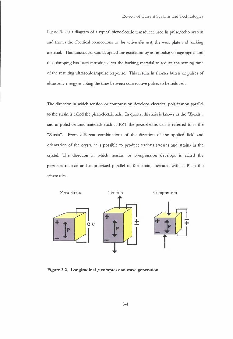
The direction in which tension or compression develops electrical polarization parallel
to the strain is called the piezoelectric axis. I n quartz, this axis is knows as the "X-axis",
and in poled ceramic materials such as P Z T the piezoelectric axis is referred to as the
"Z-axis". From different combinations o f the direction o f the applied field and
orientation o f the crystal i t is possible to produce various stresses and strains in the
crystal. The direction in which tension or compression develops is called the
piezoelectric axis and is polarized parallel to the strain, indicated wi th a T ' in the
schematics.
Zero-Stress Tension Compression
I
2 I
Figure 3.2. Longitudinal / compression wave generation
3-4

Review o f Current Systems and Technologies
Zero-Stress Shear-Stress Shear-Stress • < •
Figure 3.3. Transverse / shear wave generation
Schematic representations o f the cross-section o f typical piezoelectric crystals are
presented in Figure 3.2. and 3.3. The figures indicate that wi th a positive applied
voltage perpendicular to the piezoelectric axis, a longitudinal polarized crystal expands.
I f however the electric field is applied parallel to the piezoelectric axis, a shear motion is
induced [2]. Under a negative applied voltage, the motion is opposite; the longitudinal
crystal contracts, the shear crystal shifts in the opposite direction.
Piezoelectric transducers can be used to excite a variety o f modes into the test sample.
The four principle modes are longitudinal, shear, surface and in thin materials, plate
waves. However, a major factor that determines the amount o f energy transmitted in
and out o f the material are the acoustic impedances o f the different components o f the
system. Thus, the coupling medium between the transducer and the sample requires
consideration. The primary function o f the coupling medium is to provide a high
degree o f mechanical coupling, and in contact testing, must be thin to have minimum
effect o f the acoustic wave [3]. The reflection coefficient o f an air/steel boundary is
0.98, whereas using water as a couplant reduces this value to 0.94 (Section 5.6.) showing
that water, as a couplant is more efficient [1].
3-5

Review o f Current Systems and Technologies
Thus, these transducers are often used in automatic water immersion systems or a water-based gel is used for manual systems. Water couplant cannot support shear waves and thus only longitudinal waves wil l transmit into the material.
3.2.3. Electromagnetic Acoustic Transducers ( E M A T )
A n E M A T is a non-contact device that generates and detects ultrasound in electrically
conducting or ferromagnetic materials [4]. Thus in this case, the ultrasound is
generated directly within the material and the acoustic impedance o f the medium
between the transducer and sample is not relevant although the electromagnetic
properties are.
There are two types o f E M A T , one is based on the Lorentz force and can be used in
non-ferromagnetic materials, and the other type is based on magnetostriction and can
be used for magnetic materials and those that exhibit magnetostriction.
I n the Lorentz type, a coil is used to create a radio frequency signal that induces an
eddy current density directly into the conducting sample, which has components
perpendicular to an applied dc magnetic field. A Lorentz force is thus produced as
shown in equation. 3.1. resulting in small mechanical vibrations and hence an elastic
wave propagates into the volume o f the material, or along the surface. The use o f an
E M A T for the detection o f ultrasound works via an inverse process, where motion o f
the surface induces current into the coil. The direction o f the magnetic field also
determines whether shear or compression waves wi l l be detected at the receiver [5].
F = JXB [3.1]
3-6

Review o f Current Systems and Technologies
Magnet
E M A T Coi l Circuit
• L o r e n
Magnetic Field
Figure 3.4. Diagram of E M A T showing relevant forces
The second type o f E M A T is based on magnetostriction in ferromagnetic materials. As
wi th the Lorentz type, a coil is used to create a radio frequency (RF) field, which
produces magnetic flux changes in the material. I f a dc magnetic field is applied parallel
to the surface o f the sample, then the RF field generated causes the magnetic domains
to align. This effect gives rise to a change on dimensions known as magnetostriction
[6] . These produce a series o f tensile and compressive strains hence producing an
elastic wave. Regardless o f the generation method the RF coupling is dependent upon
the l i f t - o f f distance between the E M A T and the part. I t is therefore important to keep
the E M A T within close proximity to the object being tested (~ 1 mm) limiting the use
o f an E M A T to flat or mildly curving surfaces [7]. When an E M A T transmitter is
placed near an electrically conducting material, not necessarily in contact wi th ,
ultrasonic waves are launched in the material through the reaction o f induced eddy
currents (see Chapter 4.) and static magnetic fields (Lorentz forces). This eliminates the
problems associated with acoustic coupling to the metal part under examination as the
electro-mechanical conversion takes place direcdy within the electromagnetic skin
depth o f the material surface. Therefore, an E M A T facilitates non-contact operation
3-7
Review o f Current Systems and Technologies
and enable inspection at elevated temperatures [8], on moving objects, in vacuum or oily or rough surfaces and also in remote and hazardous locations.
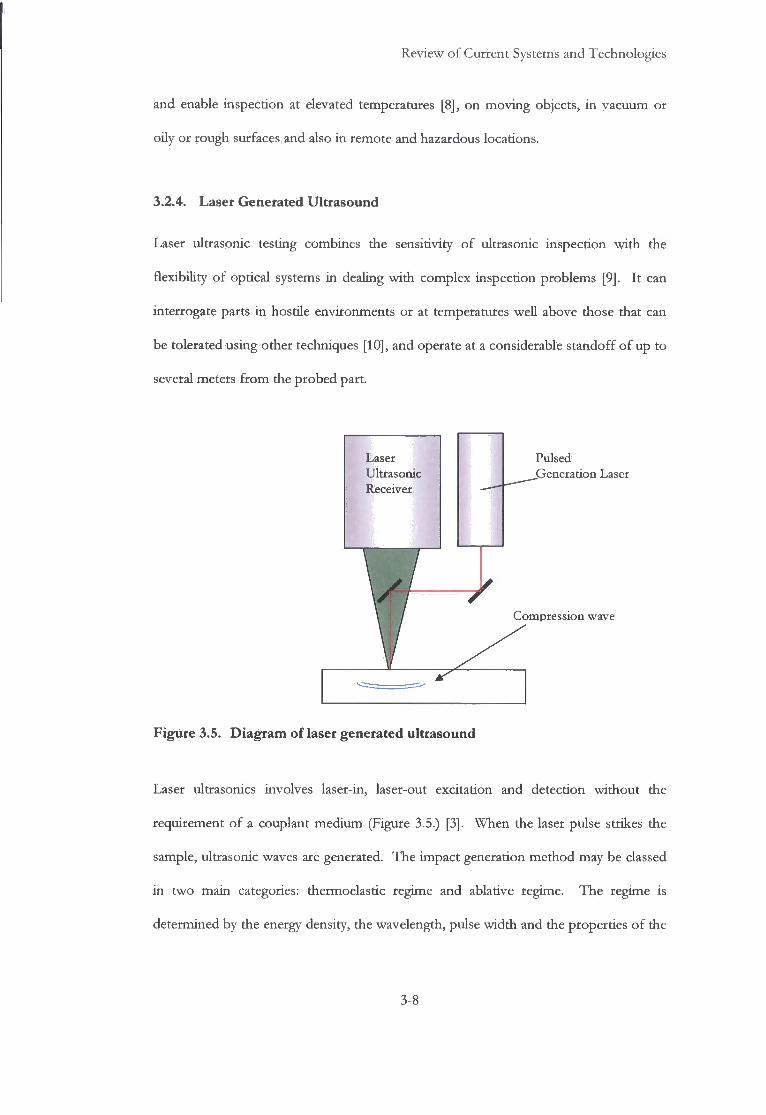
3.2.4. Laser Generated Ultrasound
Laser ultrasonic testing combines the sensitivity o f ultrasonic inspection with the
flexibility o f optical systems in dealing wi th complex inspection problems [9]. I t can
interrogate parts in hostile environments or at temperatures well above those that can
be tolerated using other techniques [10], and operate at a considerable standoff o f up to
several meters f r o m the probed part.
Ultrasonic Pulsed Generation Laser
Compression wave
Figure 3.5. Diagram of laser generated ultrasound
Laser ultrasonics involves laser-in, laser-out excitation and detection without the
requirement o f a couplant medium (Figure 3.5.) [3]. When the laser pulse strikes the
sample, ultrasonic waves are generated. The impact generation method may be classed
in two main categories: thermoelastic regime and ablative regime. The regime is
determined by the energy density, the wavelength, pulse width and the properties o f the
3-8

Review o f Current Systems and Technologies
material under examination. I n the case o f ablation, a laser source is chosen with a wavelength that wi l l have sufficient energy density to cause vaporization or ablation o f the surface o f the material [11]. The recoil that follows the material ejection o f f the surface predominandy produces longitudinal force at normal incidence to the material surface; but also produces shear waves, and surface following waves. Laser ultrasound generated in the thermoelastic regime produces a buried ultrasonic source wi th a constraining effect o f the material above i t , which induces longitudinal ultrasonic wave at normal incidence (Figure 3.5.) When the reflected ultrasonic wave reaches the surface o f the sample, a separate laser ultrasonic receiver (interferometer) is used for detection o f the ultrasonic wave. The resulting surface displacement is measured wi th the laser ultrasonic receiver based upon an adaptive interferometer.
3.2.5. Inspection Techniques
In ultrasonic testing, high-frequency sound waves are transmitted into a material to
detect imperfections or to locate discontinuities in material properties. The frequency
utilised depends on factors such as the attenuation as the wave travels through the
material under test, dispersion and resolution o f the discontinuity. Ultrasonic
inspection can be utilised for several purposes including flaw detection, material
evaluation, and dimensional measurements. When an ultrasonic wave is introduced
into a material i t has four principle modes o f propagation, longitudinal, shear, surface,
and in thin materials, plate waves. The first two modes can exist in the bulk materials
and are therefore best suited to the internal investigation of a material. T o reduce the
number o f modes further some systems employ water coupling since water does not
support shear waves [12], leaving only longitudinal waves. The way, in which sound
waves propagate through materials, and the orientation o f the area under inspection,
3-9

Review o f Current Systems and Technologies
dictate the ultrasonic technique employed. These techniques fall into two main categories, and are pulse/echo and through transmission, all other methods o f ultrasonic defect detection are adaptations and elaborations o f these two main categories.
3.2.6. P u l s e / E c h o
This is the most commonly used ultrasonic testing technique, whereby sound is
introduced into a test object via a dual-purpose transmitter/receiver probe. The signal
is then reflected f r o m any suitably orientated internal imperfections or the geometrical
surfaces o f the test object, and returns to the same transmitter/receiver probe. The
two-way transit time measured is divided by two to account for the return transit path
and multiplied by the velocity of sound in the test material. The result is expressed in
the relationship:
d = v t / 2 [3.2.]
where
d = the distance f rom the surface to the discontinuity in the test piece
v = the velocity o f sound waves in the material
t = the measured round-trip transit time
When a suitably orientated discontinuity is in the path o f an ultrasonic pulse, a
percentage o f the pulses energy wil l reflect back to the probe f r o m the surface o f the
flaw. The reflected signal is then transformed via the receiving probe back into
electrical signal to the ultrasonic flaw detector where it can be then displayed on a
3-10

Review o f Current Systems and Technologies
screen. Signal transit time can be directly related to the distance that the signal travelled. This echo signal can then be processed and information about the reflecting discontinuity, such as its location, size, and orientation, can be determined [13]. There are several methods o f displaying the ultrasonic signal, however the three most widely employed methods are A-scan, B-scan and C-can, the most commonly used o f which is the A-scan. A n A-scan plots signal amplitude against signal transit time through the medium (Figures 3.6. and 3.7.) and is then displayed as a single signal path. Because o f this use o f transit time, an A-scan can also be employed for material thickness measurements.
Probe
z 7 Defect
/
Figure 3.6. Diagram of A-scan showing defect in the core of the material
100
90
80
70
60
50 Defect 40
Defect
30
20
10
0
0 5 10 15 20 25 30 35
Time us
Figure 3.7. Representation of an A-scan showing initial pulse, defect in cote of
the material and back-wall echo.
3-11

Review o f Current Systems and Technologies
The B-Scan is a multi-signal path display, and can be visualized as a transverse cross-
sectional view f r o m the top to the bottom o f the component. As the probe is moved,
the A-Scan signals are recorded and plotted according to probe position. The response
f rom a defect wi l l be plotted along the beam axis even when it does not lie on i t ,
causing arc shaped indications on the B-Scan image, owing to the beam divergence.
These characteristic arcs vary in shape and size according to the width o f the ultrasonic
beam at different depths within the material and the defect encountered. B-scans are
generally displayed in greyscale; where intensity is proportional to the amplitude o f the
signal see Figure 3.8. and 3.9. The B-scan is less practical for non-destructive testing
where large volumes are to be examined, as they require a comparatively long scanning
time when compared to an A-scan [3].
Direction o f probe movement Direction o f probe movement
Defect
Defect
Back-wall
Figure 3.8. Diagram of B-scan test Figure 3.9. Representation of B-scan
showing probe movement and display showing probe and
defect defect position
3-12

Review o f Current Systems and Technologies
The C-scan is essentially a plan view o f the scanned material. The display is similar to
that o f a B-scan, in that the intensity displayed is proportional to the amplitude o f the
reflected signal. In sophisticated systems, digital signal processing (DSP) can be applied
to the signal facilitating filtering and signal manipuladon to givie clearer and more
readily identifiable results (Figures 3.10. and 3.11.)
I'robe
/ t Defects
Delects
Figure 3.10. Representation of C-scan Figure 3.11. T h e C-scan display with probe path and defects. defect reconstruction.
3.2.7. Through Transmission
I n this method ultrasonic energy is introduced into a test object by one probe,
propagates through the test object and received by a second transducer, usually on the
opposite side o f the test object. This method requires considered calibration prior to
any investigation as i t relies on the changes in received signal amplitude as indications
o f variations in material continuity.
3-13

Review o f Current Systems and Technologies
3.2.8. Phased Array
t = 0
•
Figure 3.12. Diagram of electronic
focusing, showing how
electronic delay is used to focus
the beam [14].
t = 0
NroJi t l t m r l
Figure 3.13. Diagram electronic beam
steering by applying electronic
delay [14].
The Phased Array concept is based on the use o f transducers made up o f individual
elements that can each be independendy driven. Each probe is made up o f a large
number o f simple probes, between 10 and several hundred [5], organized in linear,
annular, circular or matrix arrays, used as transmitters and/or receivers o f ultrasonic
waves [14]. Excitation o f each the transducer elements can be individually controlled
and exited wi th different timing delays, facilitating electronic sound-field steering, this
permits electronic scanning (beam sweeping), focusing and deflection (beam steering)
to be carried out (Figures 3.12. and 3.13.).
These phased array probes are connected to specially adapted pulser/receiver drive
units enabling independent or simultaneous pulse emission and reception along each
channel. Initial costs for the electronics and the development o f the software required
for the implementation o f a phased array systems, are more expensive than that o f
conventional ultrasonic counterparts. Also, phased array probes are more expensive
than standard ultrasonic transducers and each probe is generally application specific
[15].
3-14

Review of Current Systems and Technologies
However as more applications become commonplace, it is expected that demand for phased array systems and certain array probes will rise. The use of phased array systems in industry is expected to increase over time. This is to facilitate a reduction of inspection times and to address the inspection problems associated with complex component geometries that are not feasible with conventional methods [16,17].
3.2.9. Time of Flight Diffraction (TOFD)
Time-of-flight diffraction (TOFD) technique is based on forward-scattered diffraction
of an ultrasonic wave at the tips of discontinuities. This is in contrast to conventional
pulse echo techniques that rely on directly reflected signals from internal structures [18].
The T O F D technique as an ultrasonic NDT technique was first described and put into
practical use by Dr. Maurice G. Silk in 1977 [19]. The T O F D technique was refined
and developed over a period of years by Silk and his co-workers at the Atomic Energy
Authority's Harwell Laboratory.
The technique uses two probes in a transmitter-receiver arrangement, the probes
having a small active element to give wide beam spread angle. Broad beam probes are
used so that the entire crack area is flooded with ultrasound and, consequendy, the
entire volume is inspected using a single scan pass [20]. The technique requires the two
probes to be placed facing each other and approximately equidistant from the flaw.
With the location of the discontinuity being determined by the variation in propagation
times of the ultrasonic waves at the receiver probe. Mondal et.al. (2000) state that the
probe frequency should be 10 MHz or higher [20], because as Charlesworth et.al (2000)
state the accuracy of the measurement increases with that of the frequency [21], and
angled at between 45 to 70 degrees [22].
3-15
Review of Current Systems and Technologies
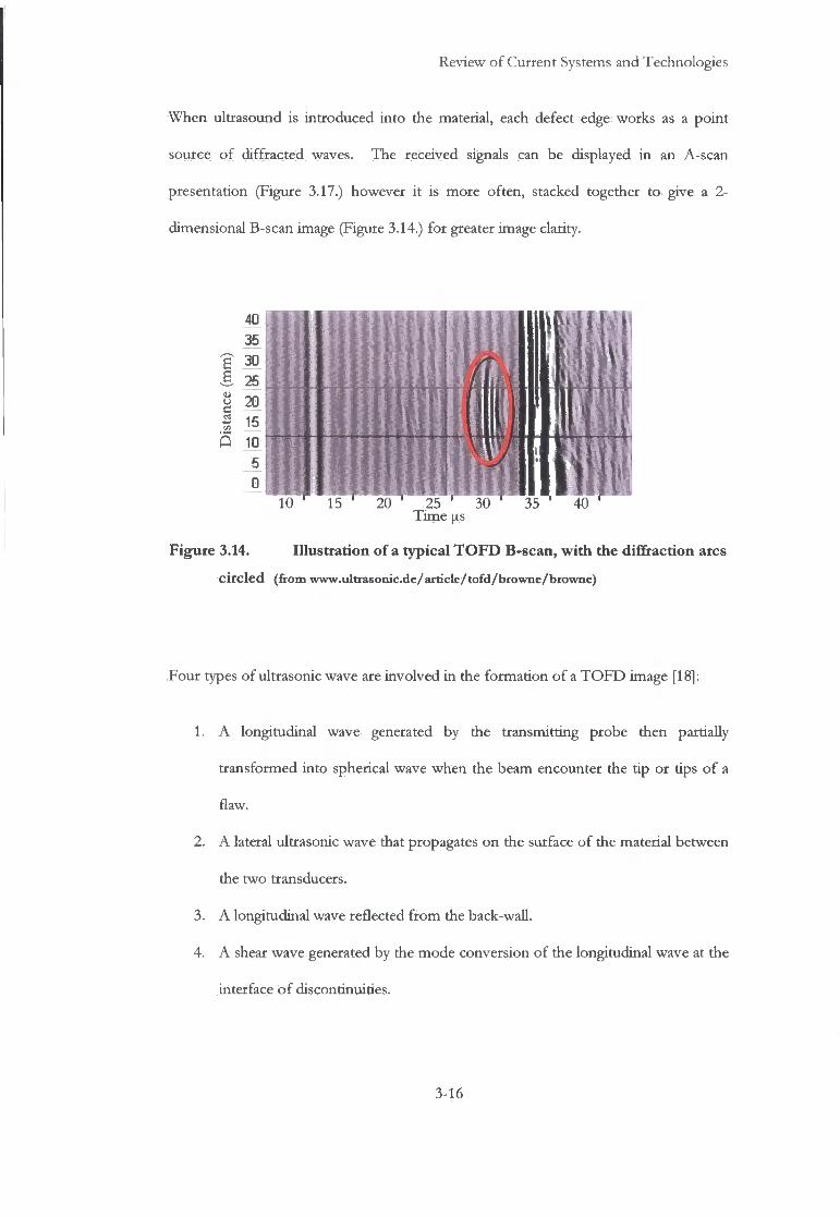
When ultrasound is introduced into the material, each defect edge works as a point source of diffracted waves. The received signals can be displayed in an A-scan presentation (Figure 3.17.) however it is more often, stacked together to give a 2-dimensional B-scan image (Figure 3.14.) for greater image clarity.
40 35
30 25
•-J
y 20
mm 15 Q 10 V
I :
_ ; , - WW • I 1 10 20 25 30 35 40 15 Time us
Figure 3.14. Illustration of a typical T O F D B-scan, with the diffraction arcs
circled (from www.ultrasonic.de/article/tofd/browne/browne)
Four types of ultrasonic wave are involved in the formation of a T O F D image [18]:
1. A longitudinal wave generated by the transmitting probe then partially
transformed into spherical wave when the beam encounter the tip or tips of a
flaw.
2. A lateral ultrasonic wave that propagates on the surface of the material between
the two transducers.
3. A longitudinal wave reflected from the back-wall.
4. A shear wave generated by the mode conversion of the longitudinal wave at the
interface of discontinuities.
3-16

Review of Current Systems and Technologies
Transmitted Wave
Reflected Wave
Through Transmitted Wave
Diffracted Wave at Upper Crack Tip
Diffracted Wave at Lower Crack Tip
Figure 3.15. Diagram showing ultrasound and crack interaction
(www.ndt.net/ndtaz/ndtaz.php)
The theory of the spherical wave is that of a wave front propagating from a relatively
small source, like that of the surface of an expanding soap bubble, i.e. a wave in which
points of the same phase lie on the surfaces of concentric spheres.
Charlsworth et.al (2002) state that it is preferable to use compression waves, because of
their earlier arrival time. However as shear waves travel at approximately half the
velocity of a compression wave, they can offer enhanced resolution [21]. The slower
speed also means that the signal of interest could arrive amongst other spurious signals,
including mode-converted compression waves, and compression waves that have
travelled greater distance. The locations of the tips of the crack are determined from
the time differences between the lateral wave, and the pulses following the paths, PI +
P2 (t,) and P3 + P4 (t 2 ) From the detected positions and times the dimensions of the
discontinuity can be determined. The following equations are for the arrival times of
the various signals from Figures 3.16. and 3.17.
i
3-17

Review of Current Systems and Technologies
IS
Lateral wave 4L
d PI ra
ii
Baclcwall echo
BackwalJ
Figure 3.16. Diagram showing twin probes and signal paths of a typical T O F D
scan
th
u 2 « 0 a, 2 6 a
Mode Time (arbitrary) converted pulse
Figure 3.17. A-scan from Figure 3.16.
3-18

Review of Current Systems and Technologies
When the defect is at normal incident to the surface and the defect is centrally positioned between the probes, as in Figure 3.16. the following equations apply: Time of surface (lateral) wave
25 t L = — [3.3.]
Time to top of defect (PI + P2)
2>/S2+d
Time to bottom of defect (P2 + P4)
_2Vs 2 +(d + a) 2
U ~ C [3.5.]
Time of Backwall echo
_ 2 V S 2 + H 2
*bw = £ [3-6-]
Where
a = defect size
d = defect depth below surface
H = material thickness
C = velocity of relevant wave mode (Longitudinal or Transverse)
S = V2 probe separation distance
The following equations refer to Figures 3.16. and 3.17. and give the depth of defect
below the surface and the defect size respectively:
Defect depth below surface
d = ^ V c 2 t f - 4 S 2 [3.7.]
3-19
Review of Current Systems and Technologies
Defect size
t j - 4 S - d [3.8.]
T O F D has several advantages over other ultrasonic techniques, in that, depth sizing is
very accurate and the defect height can be exacdy determined. An exception to this is
that the technique is not effective at detecting or sizing defect lying parallel to the
inspection surface [23]. A disadvantage of T O F D is that diffraction waves are low in
amplitude than direct reflection waves and therefore the sensitivity to flaw detection is
correspondingly lower in amplitude. Also the defects can only be realized if the
amplitude and phase of the diffracted ultrasound can be reliably interpreted [24].
T O F D has been successfully applied for testing a wide range of steel plates and
pipelines thicknesses. However according to Charlesworth et.al (2002) crack sizing
results performed with ultrasonic methods on a thick-walled pressure vessel weld,
demonstrated that it is uncertain if T O F D is a reliable method for the detection of
cracks or sharp grooves at the inner walls of pipe work or vessels [21]. There is
however no doubt of the potential for Time-of-flight diffraction used as an adjunct to
other techniques to assist with defect characterisation, location and sizing.
3.2.10. Synthetic Aperture Focusing Technique (SAFT)
The Synthetic aperture focusing technique (SAFT) is based on geometrical reflection
[25] of the ultrasound, and is essentially a digital signal processing technique (DSP)
employed for ultrasonic testing. It provides an accurate measurement of the spatial
location and extent of flaws contained within components [26]. SAFT can be split into
two sub-categories that of Conventional SAFT and Multi-SAFT.
3-20
Review of Current Systems and Technologies
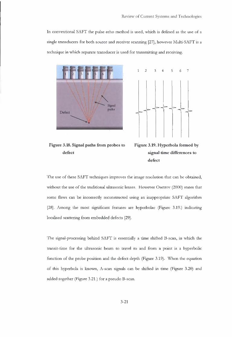
In conventional SAFT the pulse echo method is used, which is defined as the use of a single transducers for both source and receiver scanning [27], however Multi-SAFT is a technique in which separate transducer is used for transmitting and receiving.
1
\ Signal
paths Defect - r
Figure 3.18. Signal paths from probes to Figure 3.19. Hyperbola formed by
defect signal time differences to
defect
The use of these SAFT techniques improves the image resolution that can be obtained,
without the use of the traditional ultrasonic lenses. However Osetrov (2000) states that
some flaws can be incorrectly reconstructed using an inappropriate SAFT algorithm
[28]. Among the most significant features are hyperbolae (Figure 3.19.) indicating
localised scattering from embedded defects [29].
The signal-processing behind SAFT is essentially a time shifted B-scan, in which the
transit-time for the ultrasonic beam to travel to and from a point is a hyperbolic
function of the probe position and the defect depth (Figure 3.19). When the equation
of this hyperbola is known, A-scan signals can be shifted in time (Figure 3.20) and
added together (Figure 3.21.) for a pseudo B-scan.
3-21
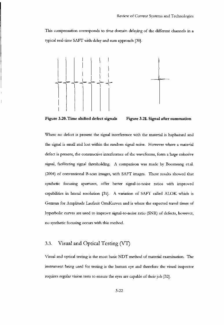
Review of Current Systems and Technologies
This compensation corresponds to time domain delaying of the different channels in a typical real-time SAFT with delay and sum approach [30].
Figure 3.20. Time shifted defect signals Figure 3.21. Signal after summation
Where no defect is present the signal interference with the material is haphazard and
the signal is small and lost within the random signal noise. However where a material
defect is present, the constructive interference of the waveforms, form a large cohesive
signal, facilitating signal thresholding. A comparison was made by Boomsang et.al.
(2004) of conventional B-scan images, with SAFT images. These results showed that
synthetic focusing apertures, offer better signal-to-noise ratios with improved
capabilities in lateral resolution [31]. A variation of SAFT called A L O K which is
German for Amplitude Laufzeit OrtsKurven and is where the expected travel times of
hyperbolic curves are used to improve signal-to-noise ratio (SNR) of defects, however,
no synthetic focusing occurs with this method.
3.3. Visual and Optical Testing (VT)
Visual and optical testing is the most basic NDT method of material examination. The
instrument being used for testing is the human eye and therefore the visual inspector
requires regular vision tests to ensure the eyes are capable of their job [32].
3-22

Review of Current Systems and Technologies
The visual examiners follow various procedures that range from simply looking at a part with the naked eye, to see i f surface defects are visible, to using a Borescope (Endoscope) to gain an image from an inaccessible location (Figure 3.22.) as the main point of visual testing is that the inspector must be able to see the surface being tested.
Figure 3.22. Simple magnifying
Borescope
Figure 3.23. Camera Borescope with
image rectifier
There are several problems associated with the use of this equipment, including
eyestrain and image distortion, due to the wide angled objective lens as in Figure 3.22.
However, the use of computer controlled camera systems can be programmed to
automatically correct this distortion [33] (Figure 3.23). These systems can also be
automated and programmed to locate, identify and measure the features of an inspected
component.
3.4. Radiography Testing (RT)
Volumetric nondestructive testing (NDT) is typically performed in industry using either
radiography or ultrasonics. Radiography having the disadvantages that it can be a safety
hazard and is poor at detecting the more critical planar discontinuities [15].
3-23
Review of Current Systems and Technologies
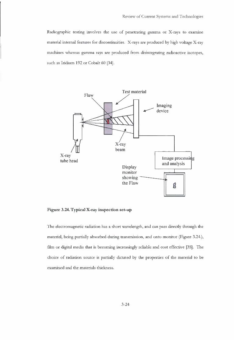
Radiographic testing involves the use of penetrating gamma or X-rays to examine material internal features for discontinuities. X-rays are produced by high voltage X-ray machines whereas gamma rays are produced from disintegrating radioactive isotopes, such as Iridium 192 or Cobalt 60 [34].
Flaw Test material
X-ray tube head
X-ray beam
Display monitor showing the Flaw
Imaging device
Image processing and analysis
8
Figure 3.24. Typical X-ray inspection set-up
The electromagnetic radiation has a short wavelength, and can pass direcdy through the
material, being partially absorbed during transmission, and onto monitor (Figure 3.24.),
film or digital media that is becoming increasingly reliable and cost effective [35]. The
choice of radiation source is partially dictated by the properties of the material to be
examined and the materials thickness.
3-24

Review of Current Systems and Technologies
St Figure 3.25. Photograph of threaded pipe Figure 3.26. Radiograph of threaded pipe
showing defect
Also gamma radiation sources have the advantage of portability, which makes them
ideal for use in site working. The resulting shadowgraphs display the internal features
of the inspected part. Material thickness and density changes are displayed as lighter or
darker areas on the film, with the darker areas of the radiograph representing internal
voids in the component (Figure 3.26.).
As Griffiths (2001) states [36], radiography on an industrial site poses a number of
safety challenges that are frequently not adequately addressed. X-rays and gamma rays
are very hazardous and can damage living tissue. To ensure there are no hazards to
personnel, precautions must be taken, and a radiography inspection should be
performed inside a protective enclosure or with appropriate barriers and warning
signals.
3.5. Magnetic Particle Inspection (MPI)
The Magnetic Particle Inspection N D T method is achieved by inducing a magnetic
field, within a ferromagnetic material. MPI can be used for detection of surface-
breaking or near-surface cracks, blowholes, and non-metallic inclusions etc. However,
i f the crack runs parallel to the magnetic field, there is little disturbance to the magnetic
field and it is unlikely that the crack will be detected.
3-25

Review of Current Systems and Technologies
For this reason the component is magnetised in more than one direction and at 90° to each other. Under optimal conditions, and with good surfaces, detection of defects of about 0.5mm long can be achieved. The sensitivity of MPI depends on the magnetisation method and on the electromagnetic properties of the material tested as well as on the size, shape and orientation of the defect [37].
Crack Maenetic Particles Magn /
N 5 N S
Figure 3.27. Billet with crack showing the flux leakage field and effective poles
The surface is dusted with iron particles that can be either dry or be suspended in liquid
and are generally brightly coloured. I f the material has no flaws, most of the magnetic
flux is concentrated below the material's surface. However, i f a flaw is present, such
that it interacts with the magnetic field, the flux is distorted locally and the flux appears
to leak from the surface of the specimen in the region of the flaw as shown in Figure
3.27.
Surface and near-surface flaws produce magnetic poles or distort the magnetic field in
such a way that the iron particles are attracted and concentrated in these areas. This
produces a visible indication of a defect on the surface of the material and is much
easier to detect than the actual crack and this is the basis for magnetic particle
inspection.
3-26
Review of Current Systems and Technologies
The demagnetisation of the component is often specified after MPI to avoid the build up of particles. This demagnetisation is achieved by subjecting the component to a continuously alternating and reducing magnetic field, with the start point of the cyclic demagnetisation being, as high, or higher than that of the magnetizing field.
3.6. Eddy Current Testing (EC)
Eddy currents are created through electromagnetic induction and take their name from
the "eddies" that are formed when a liquid or gas flows in a circular path around
obstacles. As an alternating current flows through a coil a dynamic expanding and
collapsing magnetic field forms, and when a conductive material is placed within close
proximity electromagnetic induction occurs and eddy currents are induced in the
material. A secondary magnetic field is generated by the eddy current, which opposes
the coil's magnetic field as shown in Figure 3.28.
Concentrated mainly at the surface of a material, eddy currents can dierefore only be
used to detect surface and near surface defects, due to the skin effect [38]. Skin depth
is a term used for the depth at which the amplitude of an electromagnetic wave
attenuates to 1/e of its original value or 37% of it value at the surface [39]. The skin
depth for plane waves 8 can be calculated using equation 3.9.
3-27

Review of Current Systems and Technologies
Alternating Current
Primary Magnetic Field
Secondary Magnetic Field
Probe Coil
Eddy Currents
Conductive Material
Figure 3.28. Diagram of the generation of eddy currents
\a>M [3.9]
wi here p — resistivity of conductor
CO — angular frequency of current = 2n X frequency
ju - absolute magnetic permeability of conductor
3-28

Review of Current Systems and Technologies
The skin effect is a fundamental electromagnetic phenomenon and is dependent upon specimen conductivity permeability and the operating frequency. This is explained by Lenz's Law, which states "when an EMF is induced in a conductor by any change in the relation between the conductor and the magnetic field, the direction of the EMF is such as to produce a current whose magnetic field will oppose the change" [40]. The skin effect has been widely used for non-destructive testing using inductance coils and magnetic/eddy current techniques for both sub-surface inspection [41] and for crack detection [42].
For most N D T inspection applications, eddy current probe frequencies are in the range
1kHz to 3MHz are used with the lower frequencies giving deeper penetration, typically
between 5 [xm and 1 mm. The presence of any discontinuity will cause a change in
eddy current flow and a corresponding change in the phase and amplitude of the
measured eddy current [43]. Eddy currents are also affected by the electrical
conductivity and magnetic permeability of a material, which makes it possible to
distinguish between various conductive materials based on these properties.
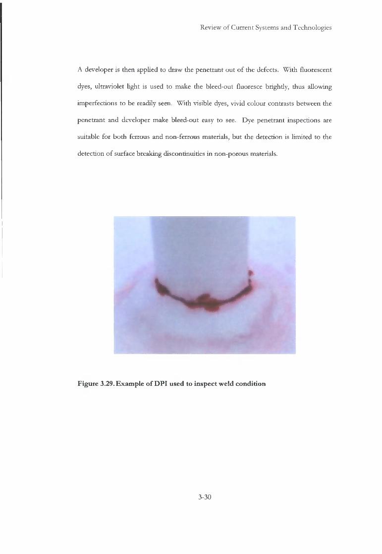
3.7. Dye Penetrant Inspection (DPI)
The purpose of the dye penetrant inspection is to increase the visible contrast between
a discontinuity and the background material. This is achieved by applying a penetrating
liquid that contains a visible or fluorescent dye, as shown in Figure 3.29. Excess
solution is then removed from the surface of the object but leaving it in surface
breaking defects.
3-29
Review of Current Systems and Technologies
A developer is then applied to draw the penetrant out of the defects. With fluorescent
dyes, ultraviolet light is used to make the bleed-out fluoresce brighdy, thus allowing
imperfections to be readily seen. With visible dyes, vivid colour contrasts between the
penetrant and developer make bleed-out easy to see. Dye penetrant inspections are
suitable for both ferrous and non-ferrous materials, but the detection is limited to the
detection of surface breaking discontinuities in non-porous materials.
Figure 3.29. Example of DPI used to inspect weld condition
3-30
Review o f Current Systems and Technologies
3.8. Conclusion
This chapter contained an overview o f the various N D T technologies and as such
covered all the methods relevant to the project. As the project remit was an immersion
ultrasonic system using piezoelectric transducers, those were discussed in greater depth.
Several o f the methods described were totally unsuitable for the interrogation o f the
core o f the billet, including Dye Penetrant Inspection, Magnetic Particle Inspection,
Eddy Current, and Visual Testing. As all o f these methods are suitable for only surface,
surface breaking, or in the case o f Eddy Current near surface defects.
The use o f Radiography for billet inspection has problems wi th the radiation
containment, as inspection should be performed inside a protective enclosure. This
would necessitate the protective enclosure allowing for the billet to traverse through
and to the next station without interruption, and have an automated defect detection
and marking system, instead o f producing radiographic images. According to Hanke
et.al. (2004) the current methods for high-speed volume data evaluation have cycle
times o f about one minute, for a defect detection size o f circa 15 cm [44], and this is an
impractical throughput and defect detection size for economic and competitive
production o f steel.
The use o f an E M A T for automated billet inspection would eliminate the need for an
immersion system and the potential problems that they entail, predominantly air
entrapment. However as an E M A T is required to be in close proximity (~ 1 mm) [7]
with the material they a inspecting, this would be problem wi th a moving billet where
the stand o f f distance is constandy changing due to material 'snaking'.
3-31
Review o f Current Systems and Technologies
Also they are less efficient at converting electrical energy into sound, which would
prove problematic when testing a large cross-sectional material or a highly attenuating
material as performance decreases with distance [3].
The expenditure on a laser ultrasonic system capable o f scanning a 75mm square
section billet, moving at 1 m/s , in a steel mi l l would be excessive. That a laser system
could complete the examination is not in question, however the required financial
ouday would necessitate a marked increase in material throughput. Also because o f the
use o f lasers, the inspection area may require being in an enclosure or be in a limited
access area. However according to Kline (1996) laser-based ultrasound is definitely not
a solution to all problems, but i t can be very powerful in the right application, especially
i f surface ablation is allowed [10].
3-32
Review o f Current Systems and Technologies
3.9. References
1. Hellier, C.J., Handbook of Nondestructive Evaluation. 2001, New York, U.S.A.: McGraw-Hil l .
2. Johnston, P.H. Free Response of Piezoelectric Crystals in Series and in Parallel, in Review of Progress in Quantitative Nondestructive Evaluation. 2003, p. 729-736.
3. Birks, A.S. and R.E. Green Jr., Ultrasonic Testing. 2nd ed. Nondestructive Testing Handbook, ed. P. Mclntire. Vo l . 7. 1991, Baltimore, Maryland, U.S.A.: American Society for Nondestructive Testing. 893.
4. Dixon , S., et al., A Laser - EMAT System for Ultrasonic Weld Inspection. Ultrasonics, 1999. 37(4): p. 273-281.
5. Krautkramer, J. and H . Krautkramer, Ultrasonic Testing of Materials. 1990, New York: Springer-Verlag. 677.
6. Marton, L . and C. Marton, Ultrasonics. Methods o f Experimental Physics, ed. P.D. Edmonds. V o l . 19. 1981, London: Academic Press Inc. 619.
7. Klein, M.B . and T. Bodenhamer, Laser ultrasonics, in Industrial Laser Solutions. 2004,19(12). http://ils.pennnet.com/home.cfm.
8. Light, G . M . and J. Demo, An Evaluation of EMAT Technology for High-Temperature NDE. 1998, www.ndt.net/article/0398/light/light.htm.
9. Cho, H . , et al., Non-contact Laser Ultrasonics for Detecting Subsurface Lateral Defects. N D T & E International, 1996. 30: p. 301-306.
10. Klein, M.B. , Laser generated ultrasound. 1996, www.ndt.net/articlc/az/ut idx.htm.
11. Wang, X . D . , et al., Laser-generated ultrasound with an array of melting sources. Applied Physics A . Materials Science and Processing, 2000. 70(2): p. 203-209.
12. Lynnworth, L.C. and E.P. Papadakis, Ultrasonic Measurements for Process Control-Theory, Techniques, Applications. 1989, Boston: Academic Press.
13. Corneloup, G , et al., Ultrasonic image data processing for the detection of defects. Ultrasonics, 1994. 32(5): p. 367-374.
14. Poguet, J., et al., Phased Array Technology: Concepts, Probes and Applications. 2002, www.ndt.net/article/az/ut idx.htm.
3-33

Review o f Current Systems and Technologies
15. Granillo, J. and M . Moles, Portable Phased Array Applications. The N D T Technician, 2005. 4(2).
16. Anderson, M.T. , Ultrasonic Phased Array. The N D T Technician, 2003. 2(2).
17. Mahaut, S., et al., Development of phased array techniques to improve characterisation of defect located in a component of complex geometry. Ultrasonics, 2002. 40: p. 165-169.
18. Beta, F., et al. Accuracy Capability ofTOFD Technique in Ultrasonic Examination of Welds, in ASNT Spring Conference and 8th Annual Research Symposium. 1998. Orlando, U.S.A.: www.nardoni.it/Serv02knk.htm.
19. Silk, M.G. , Ultarsonic Testing - Special Techniques. The Capabilities and Limitations o f N D T , ed. P.D. Hanstead. Vo l . 5. 1988, Northampton: British Institute o f Non-Destructive Testing. 31.
20. Mondal, S. and T. Sattar, An overview TOFD method and its Mathematical Model. www.ultrasonic.de/article/v05n04/mondal/mondal.htm, 2000. 5(4).
21. Charlesworth, J.P. and J.A.G. Temple, Engineering Applications of Ultrasonic Time-of-Flight Diffraction. Second Edition ed. Ultrasonic Inspection in Engineering, ed. M.J. Whittle. 2002, Baldock: Research Studies Press Ltd . 254.
22. Ginzel, E., et al., TOFD Enhancement to Pipeline Girth Weld Inspection. N D T . Net, 1998. 3(4).
23. Baby, S., et al., Defect detection study in austenitic steel welds and the performances of different ultrasonic transducers. Insight, 2001. 43(11): p. 735-741.
24. Ravenscroft, F.A., et al., Diffraction of ultrasound by cracks: comparison of experiment with theory. Ultrasonics, 1990. 29(1): p. 29-37.
25. Frederick, J.R., Ultrasonic Engineering. 1965, London: John Wiley & Son.
26. Elbern, A . W . and L. Guimaraes. Synthetic Aperture Focusing Technique for Image Restauration. in International Symposium on NDT Contribution to the Infrastructure Safety Systems. 1999. Torres, RS Brazil.
27. Doctor, S.R., et al., SAFT the Evolution of a Signal Processing Technology for Ultrasonic Testing. N D T International, 1986.19(3): p. 163-167.
28. Osetrov, A . V . , Non-linear algorithms based on SAFT ideas for reconstruction offlaws. Ultrasonics, 2000. 38: p. 739-744.
3-34
Review o f Current Systems and Technologies
29. Schickert, M . , et al., Ultrasonic Imaging of Concrete Elements Using Reconstruction by Synthetic Aperture Focusing Technique. Journal o f Materials in Civil Engineering, 2003.15(3): p. 235-246.
30. Ylitalo, J., A fast ultrasonic synthetic aperture imaging method: application to NDT. Ultrasonics, 1996. 34: p. 331-333.
31. Boonsang, S., et al., Synthetic aperture focusing techniques in time andfrequency domains forphotoacoustic imaging. Insight, 2004. 46(4): p. 196-199.
32. Iddings, F.A., The Basics of Visual Testing. The N D T Technician, 2004. 3(3).
33. Smith, W.E. , et al., Correction of distortion in endoscope images. Medical Imaging, 1992.11(1): p. 117-122.
34. Gilbert, D.J., BINDT Yearbook 2005. 2005, Northampton: The British Institute o f Non-Destructive Testing, p. 74-75.
35. Deprins, E. Computed Radiography in NDT Applications, in World Conference on NDT. 2004. Montreal, Canada: www.ndt.net/article/wcndt2004/pdf/radiography/367 deprins.pdf.
36. Griff i ths , R. Safety Issues in the Management of Industrial Radiography, in 10th APCNDT. 2001. Brisbane, Austrailia: www.ndt.net/article/apcndtOl / papers/505 / 505.htm.
37. Lovejoy, D.J., Magnetic Particle Inspection: A practical guide. 1st ed. 1993, Norwell , U.S.A.: Kluwer Academic Publishers. 459.
38. Takagi, T., et al., Benchmark models of eddy current testing for steam generator tube: experiment and numerical analysis. International Journal o f Applied Electromagnetics in Materials., 1994. 7(3): p. 149-162.
39. Halmshaw, R., Mathematics and Formulae in NDT. 2nd ed. 1993, Northampton: The British Institute o f Non-Destructive Testing.
40. Kingsbury, R.F., Elements of Physics. 1965, Princeton, New Jersey, U.S.A.: D . Van Nostrand Co. Inc.
41. Uzal, E. and J .H . Rose, The impedance of eddy current probes above layered metals whose conductivity and permeability vary continuously. Magnetics, 1993. 29(2): p. 1869-1873.
42. Bowler, J.R., Review of eddy current inversion with application to non destructive evaluation. International journal o f Applied Electromagnetics & Mechanics, 1997. 8: p. 3-16.
3-35

Review o f Current Systems and Technologies
Bowler, J.R., Eddy-current interaction with an ideal crack. Journal o f Applied Physics, 1994. 75(12): p. 8128-8137.
Hanke, R., et al. Automated High Speed Volume Computed Tomography for Inline Quality Control, in World Conference on NDT. 2004. Montreal, Canada.
3-36
Review o f Basic Theory
Chapter 4.
Review of Basic Theory
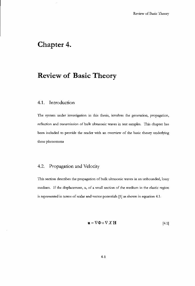
4.1. Introduction
The system under investigation in this thesis, involves the generation, propagation,
reflection and transmission o f bulk ultrasonic waves in test samples. This chapter has
been included to provide the reader with an overview o f the basic theory underlying
these phenomena
4.2. Propagation and Velocity
This section describes the propagation o f bulk ultrasonic waves in an unbounded, lossy
medium. I f the displacement, u , o f a small section o f the medium in the elastic region
is represented in terms o f scalar and vector potentials [1] as shown i n equation 4.1.
u = VO + V Z H [4.1]
4-1

Review o f Basic Theory
and is then substituted into the equation o f motion, two independent wave equations result.
2 1 d 2 u V u=—: — given u = V O
c\ dt2
[4.2]
1 S^II V 2 H = — — - given u = V x H and V H = 0
4 dt2 6
[4.3]
where equation 4.2 represents longitudinal or dilatational waves and equation 4.3 shear
or rotational waves. These two waves can only be coupled on the boundary o f the
elastic body. The parameters cL and Op represent the phase velocity o f each type o f
wave.
The general solution to these equations are:
u = Ae-aLX *eiihx-'*), u = V O
u = Be~aTX *emx~^, « = V J C H , V • H = 0 ^
where <xL and are the attenuations o f the waves as a function o f distance. For a wave
o f frequency, co, wi th a wave number, k, the velocity is given by,
a>
4-2
Review o f Basic Theory
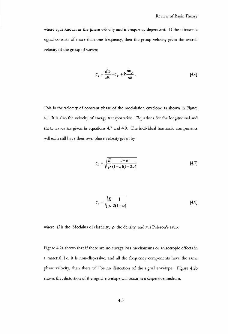
where c p is known as the phase velocity and is frequency dependent. I f the ultrasonic signal consists o f more than one frequency, then the group velocity gives the overall velocity o f the group o f waves;
d a > i d c p cv = = c „ + k — 4 . 6 1 g dk " dk L J
This is the velocity o f constant phase o f the modulation envelope as shown in Figure
4.1. I t is also the velocity o f energy transportation. Equations for the longitudinal and
shear waves are given in equations 4.7 and 4.8. The individual harmonic components
wi l l each still have their own phase velocity given by
\E_tS_ m \ p(\ + u)(\-2u)
C T = 1 - T ^ — [4-8] \P 2(1+ «)
where E is the Modulus o f elasticity, p the density and u is Poisson's ratio.
Figure 4.2a shows that i f there are no energy loss mechanisms or anisotropic effects i n
a material, i.e. i t is non-dispersive, and all the frequency components have the same
phase velocity, then there wi l l be no distortion o f the signal envelope. Figure 4.2b
shows that distortion o f the signal envelope wi l l occur in a dispersive medium.
4-3

Review o f Basic Theory
Modulation envelope (lower frequency)
Carrier wave (higher frequency)
Diagram showing group velocity [2]
Wave at t, Wave at /, 'i 2 x a. Example of wave traveling without distortion
Wave at t, Wave at 'l '2 X
b. Example of wave envelope traveling with distortion
Examples of signals in non-dispersive and dispersive media [2]
4-4

Review o f Basic Theory
4.3. Wave Propagation at Boundaries
Consider a plane stress wave p ( travelling in medium 1 approaching the boundary to
medium 2 at normal incidence. Some of wave wi l l be transmitted to medium 2 and the
rest reflected back into medium 1. The degree to which this occurs is dependent i n the
ratio o f the acoustic impedances o f the two media, ^ and Z 2 and is defined by
reflection coefficient, R and the transmission coefficient, T.
These are shown in equations 4.9 and 4.10.
R = £j_ = h^h, [ 4 9 ]
Pi Z2+Z}
T = E±= 2 Z 2 [ 4 1 0 ]
Pi Z2+Z,
Where the acoustic impedance Zx is given by
Z,=P,c, [4.11]
where p \ is the density o f the medium and c, the velocity.
Thus, i t can be seen that the larger the ratio between the two impedances, the more o f
the wave energy is reflected and less is transmitted [14]. For example, consider the
boundaries between water and steel and air and steel. Their nominal properties are
shown in Table 4.1.
4-5

Review o f Basic Theory
Table 4.1 Material properties
Material c in ms"1 p in kg m"3 Z in kPa s m 1
Water at 20°C 1480 998.2 1.483
Ai r 343 1.168 0.413
Steel mild 5900 7830 46.000
(from www.edboyden.org/ constants)
These values show that water provides a high degree o f mechanical coupling hence
more wave energy is transmitted at the water-steel interface (R=0.94), than at an air-
steel interface and, water or water-based compounds are commonly used for ultrasonic
coupling [3].
Now, consider the plane wave incident upon a boundary at an angle ac. as shown in
Figure 4.4. The angle o f the reflected wave wi l l be equal to the angle o f incidence and
the transmitted wave wi l l be refracted according to Snell's law as shown in equation
4.12.
[4.12.]
where c t is the velocity in material 1, C 2is the velocity in material 2, a; is the angle o f
incidence, ar is the angle o f reflection and ad is the angle o f refraction.
4-6

Review o f Basic Theory
Material 2 (Steel)
Velocity = q 7 a a
a Velocity = c2
Material 1 (Water)
Figure 4.3. Diagram of Snell's law for refracted angles
When a longitudinal wave propagates through a boundary, part o f the energy can
convert to a shear wave. Since shear waves have a different velocity, the angle o f
refraction wi l l be different. I f the longitudinal wave moves f r o m a slower to a faster
material as in the immersion testing o f steel, there is an angle o f incidence that creates a
90 degrees angle o f refraction for the wave. This angle is known as the first critical
angle and can be found f r o m Snell's law by putting in an angle of 90 degrees. The
resulting wave is referred to as a creep wave. However, i t has the same velocity as the
longitudinal wave. Rearranging equation 4.12. and using velocities o f 1480 ms"1 for
water and 5900 ms 1 for steel, the critical angle is:
For this reason, most angle beam transducers generate a shear wave in the test
specimen. However, there is also a critical angle for shear waves. A t this point, known
as the second critical angle, all o f the ultrasonic wave energy is either reflected away
1480 x sin 90° =14.53 0 [4.12.]
5900
f r o m the boundary or refracted into a surface shear wave or shear creep wave.
4-7

Review o f Basic Theory
4.4. Loss mechanisms
There are three main loss mechanisms in solid media, scattering, diffraction and
absorption due to internal factional losses. These can be detected primarily by
measuring the attenuation o f a reflected signal f r o m a known boundary and can be
represented mathematically by the attenuation coefficient a described in section 4.1.
Evidence of scattering can also be obtained by looking at the background noise known
as grass.
The effective diffraction loss and phase change in the field o f broadband transducers is
computed in terms o f the normalized distance travelled at the centre frequency o f the
pulse, i t this instance, 5MHz. The diffraction loss fluctuates in the nearfield wi th S
before becoming monotonic in the far field, and increasing as the logarithm o f S
(Equation 4.13) Where, ^ is the distance to the crystal, A,is the wavelength, and a is the
transducer radius [4].
S - [4.13]
However the most dominant mechanism is scattering and this occurs f r o m the fact that
the material is not strictly homogeneous. I t contains boundaries at which the acoustic
impedance changes abrupdy. I n a material wi th a very course grain structure o f a size
comparable to the wavelength o f the signal, the scatter can be visualised geometrically
[5]. A t an oblique boundary the wave is split into various reflected wave types. This
process repeats itself for each grain boundary encountered and Birks (1991) states, i t is
one o f the main sources o f loss in commercial alloys [6]. Thus, the original sound
beam is constantly sub-divided into partial waves and throughout its complex pathway
and frictional losses its energy converted into heat.
4-8

Review o f Basic Theory
I f P T is the signal power at the transmitting probe, and P R is the signal power at the receiving end then the power attenuation Ap in decibels is given by the formula,
A p = 101og 1 0(P T/P R). [4.14]
The sound attenuation increases wi th an increase in the frequency, and as the distance
increases f r o m the source. For the case o f Rayleigh scattering wi th , X > 2K D [7]
375p 2v, 3
2 3 —+ — [4.15]
27t 3 p. 2 Tf 4
a-, 2 . , 3 125p 2v,
2 3 — + — [4.16]
and for Rayleigh scattering wi th X < 2nD 3 [7]
a _\6n2
M
2Df< 1 5 2 5 v , V
[4.17]
4 ^ V 2 D / 4
210v,V a, = [4.18]
where D is the average grain diameter
4-9
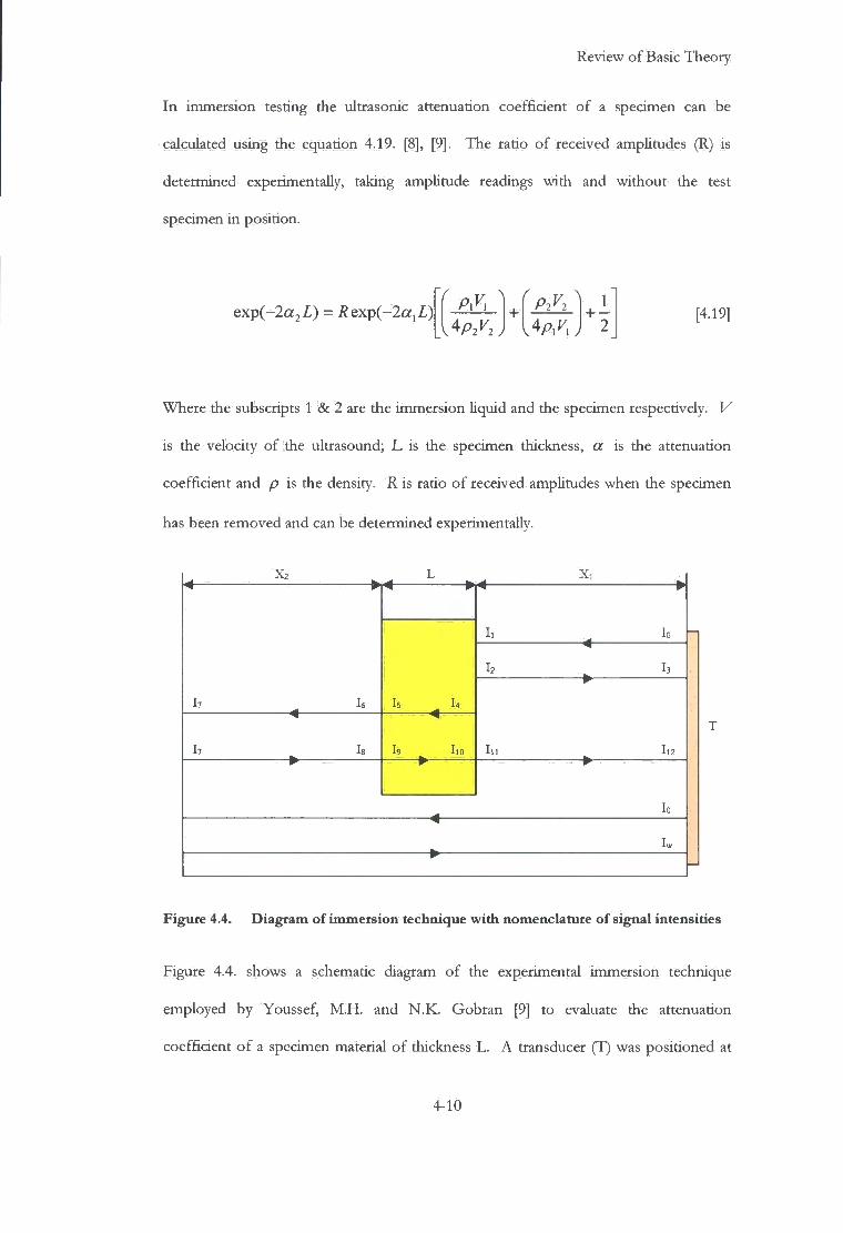
Review o f Basic Theory
I n immersion testing the ultrasonic attenuation coefficient o f a specimen can be calculated using the equation 4.19. [8], [9]. The ratio o f received amplitudes (R) is determined experimentally, taking amplitude readings with and without the test specimen in position.
exp(-2a 2 Z) = Rexpi-la^) 4p2V:
+ 2 J
PlV2 + • [4.19]
Where the subscripts 1 & 2 are the immersion liquid and the specimen respectively. V
is the velocity o f the ultrasound; L is the specimen thickness, a is the attenuation
coefficient and p is the density. R is ratio o f received amplitudes when the specimen
has been removed and can be determined experimentally.
X 2 L Xi
h Is Is U
Ii lo
h Is Is U
4
h h
h Is Is U w
111 I12 17 Is I9 I10
w
111 I12 • w w
Io
I„ w
Figure 4.4. Diagram of immersion technique with nomenclature of signal intensities
Figure 4.4. shows a schematic diagram o f the experimental immersion technique
employed by Youssef, M . H . and N . K . Gobran [9] to evaluate the attenuation
coefficient o f a specimen material o f thickness L . A transducer (T) was positioned at
4-10

Review o f Basic Theory
distance X ! f r o m the specimen on one side o f the immersion tank, wi th the specimen being a distance o f X^ f r o m the opposite tank wall. I 0 is the intensity o f the signal leaving the ultrasonic transducer, wi th I j representing the intensity o f the signal reaching the specimen, after travelling a distance o f X , . I 3 represents the intensity o f the signal reaching the transducer, after travelling a distance o f 2X, with I 1 2 representing the intensity o f the signal arriving at the transducer, after travelling a distance o f 2X,+2L+2X2.
4.5. Diffraction of Waves
Diffract ion can be generalised as the spreading o f a plane sound wave as it passes
through an aperture or the edge o f an obstacle. Therefore, when an ultrasonic wave
impinges on a discontinuity the wave is scattered by the discontinuity, and at the edge
o f the discontinuity the wave wi l l be diffracted [10]. In this way, the wave energy that
was travelling in one direction can be radiated and distributed into a wide range o f
angles, wi th a consequent reduction in the energy travelling in the original direction o f
propagation.
Shadow region Shadow region
1 l Shado\ Shadow region
Figure 4.5. Drawing showing waves diffracting around objects
4-11
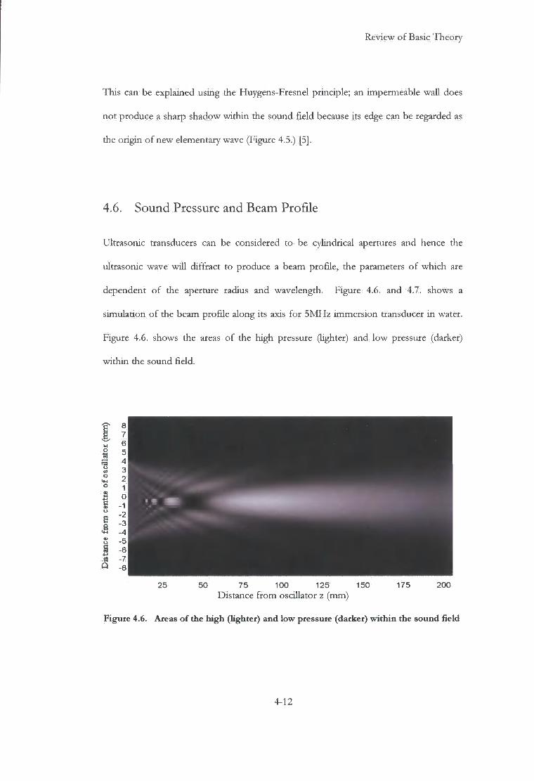
Review o f Basic Theory
This can be explained using the Huygens-Fresnel principle; an impermeable wall does
not produce a sharp shadow within the sound field because its edge can be regarded as
the origin o f new elementary wave (Figure 4.5.) [5].
4.6. Sound Pressure and Beam Profile
Ultrasonic transducers can be considered to be cylindrical apertures and hence the
ultrasonic wave wi l l diffract to produce a beam profile, the parameters o f which are
dependent o f the aperture radius and wavelength. Figure 4.6. and 4.7. shows a
simulation o f the beam profile along its axis for 5MHz immersion transducer in water.
Figure 4.6. shows the areas o f the high pressure (lighter) and low pressure (darker)
within the sound field.
8
6
'4-1
0 1 u
U -6 4-1 2
8
175 200 25 50 75 100 125 150 Distance f r o m oscillator z (mm)
Figure 4.6. Areas of the high (lighter) and low pressure (darker) wi th in the sound field
4-12

Review o f Basic Theory
1
1
1 5
1 18 35 52 69 86 103 120 137 1 54 171 188
Distance f r o m oscillator z (mm)
Figure 4.7. Plot o f the sound pressure
According to Krautkramer et al [5] the sound pressure on the axis (Figure 4.7.) is given
by the formula (Equation 4.20.) where z is the distance on the axis f r o m the centre
point o f the oscillator and D is its diameter shown in Figure 4.7.
p = p02sm
f ~ |
n 2 2
— J + z - z A V
V )
[4.20.]
4.6.1. T h e Near and Far fields
The Nearfield (N) has areas o f differing sound pressure and it extends f r o m the source
o f radiation to a point just short o f the far field or Fraunhofer zone (Figure 4.8.)
defined by the location o f the last pressure maximum as shown in Figure 4.7.
4-13
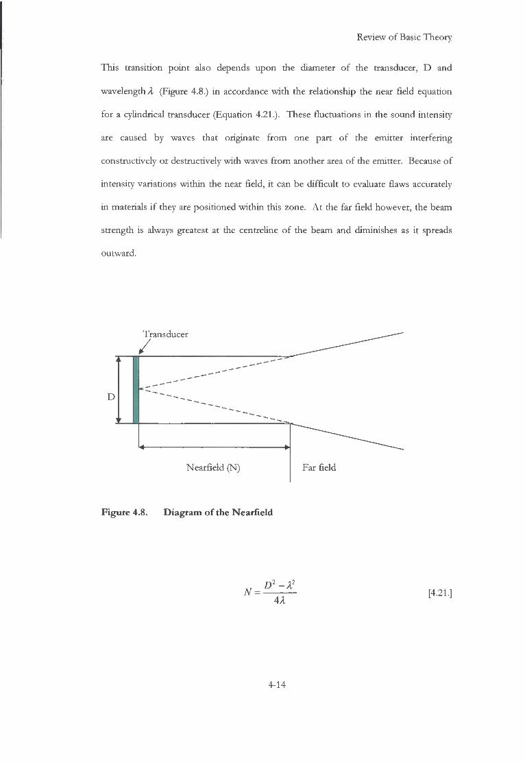
Review o f Basic Theory
This transition point also depends upon the diameter o f the transducer, D and wavelength A, (Figure 4.8.) in accordance wi th the relationship the near field equation for a cylindrical transducer (Equation 4.21.). These fluctuations in the sound intensity are caused by waves that originate f r o m one part o f the emitter interfering constructively or destructively with waves f r o m another area o f the emitter. Because o f intensity variations within the near field, i t can be diff icult to evaluate flaws accurately in materials i f they are positioned within this zone. A t the far field however, the beam strength is always greatest at the centreline o f the beam and diminishes as it spreads outward.
Transducer
/
1)
Nearfield (N) Far field
Figure 4.8. D iag ram o f the Near f i e ld
D2-X2
41 N = [4.21.]
4-14
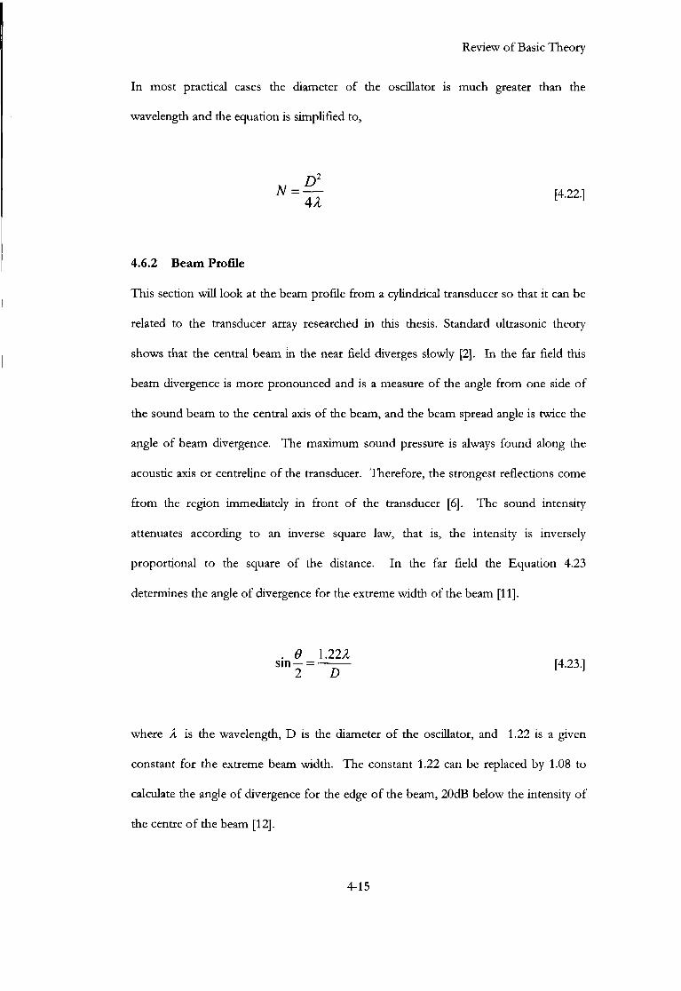
Review o f Basic Theory
I n most practical cases the diameter o f the oscillator is much greater than the wavelength and the equation is simplified to,
N = u [ 4 ' 2 2 )
4.6.2 Beam Profile
This section wi l l look at the beam profile f r o m a cylindrical transducer so that i t can be
related to the transducer array researched in this thesis. Standard ultrasonic theory
shows that the central beam in the near field diverges slowly [2]. I n the far field this
beam divergence is more pronounced and is a measure o f the angle f r o m one side o f
the sound beam to the central axis o f the beam, and the beam spread angle is twice the
angle o f beam divergence. The maximum sound pressure is always found along the
acoustic axis or centreline o f the transducer. Therefore, the strongest reflections come
f r o m the region immediately in front o f the transducer [6]. The sound intensity
attenuates according to an inverse square law, that is, the intensity is inversely
proportional to the square o f the distance. I n the far field the Equation 4.23
determines the angle o f divergence for the extreme width o f the beam [11].
. e MIX s i n - = [4.23.]
where X is the wavelength, D is the diameter o f the oscillator, and 1.22 is a given
constant for the extreme beam width. The constant 1.22 can be replaced by 1.08 to
calculate the angle o f divergence for the edge o f the beam, 20dB below the intensity o f
the centre o f the beam [12].
4-15

Review o f Basic Theory
4.7. Signal to Noise Ratio
The signal to noise ratio is defined as the ratio o f the amplitude o f an ultrasonic echo
arising f r o m the discontinuity in a material (signal V s ) , to the r.m.s amplitude o f the
background noise signal or grass ( V ) .
The signal-to-noise ratio (SNR) in decibels is given by:
SNR = 20 \ogl0(y/V) [4.24.]
This noise can arise f r o m the material characteristics, un-required ultrasonic modes and
equipment noise. Ambient noise is very often the real source, and is especially likely to
occur in automated testing installations. Several opinions arise when discussing signal
processing for enhancing the required part or suppressing the unwanted part o f the
signal, all claiming to have positive results. Enhancing the reliability o f flaw detection,
through the use o f digital signal processing [13], using contact and immersion
techniques, showed that the immersion techniques provided a greater level o f reliability.
The use o f a wavelet transform process and is stated by Chen and Shi [14], to be more
powerful than frequency filtering as a method o f enhancing reliability. However
negligible improvements were made f r o m immersion tests. There have been many
applications o f wavelet transforms in ultrasonic non-destructive testing [15, 16]. L i and
Ma [17] used a wavelet transform to identify signals o f localised defects i n bearings,
while Cho et. al. [18] applied the wavelet transform o f the digital data in deducing the
scattering o f subsurface lateral defects.
4-16
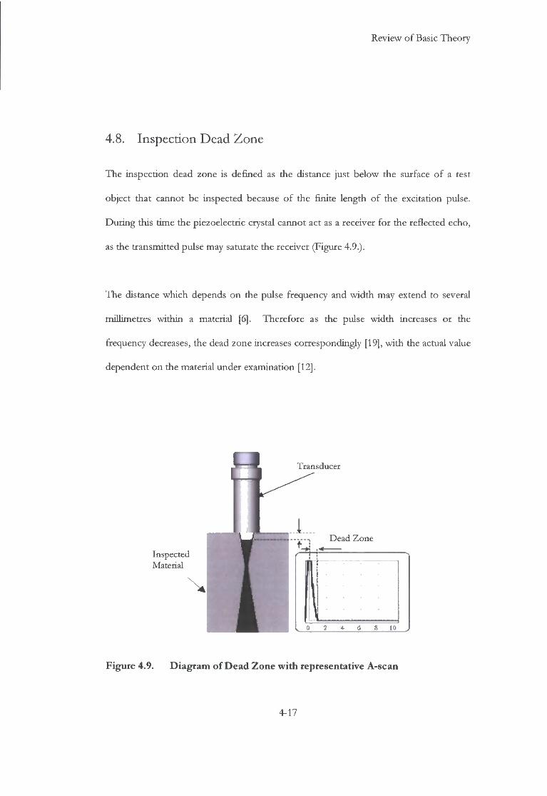
Review o f Basic Theory
4.8. Inspection Dead Zone
The inspection dead zone is defined as the distance just below the surface o f a test
object that cannot be inspected because o f the finite length o f the excitation pulse.
During this time the piezoelectric crystal cannot act as a receiver for the reflected echo,
as the transmitted pulse may saturate the receiver (Figure 4.9.).
The distance which depends on the pulse frequency and width may extend to several
millimetres within a material [6]. Therefore as the pulse width increases or the
frequency decreases, the dead zone increases correspondingly [19], wi th the actual value
dependent on the material under examination [12].
Transducer
Dead Zone
Inspected Material
i
10
Figure 4.9. D iag ram o f Dead Zone w i t h representative A-scan
4-17
Review o f Basic Theory
4.9. Summary
This chapter has given an overview o f the basic theory used in the implementation o f
the research project described in this thesis. A particular emphasis has been given to
unbounded bulk wave propagation using cylindrical transducers and the relationship
between theory and inspection terminology.
4-18

Review o f Basic Theory
4.10. References
1. Morse, P.M. and H . Feshbach, Methods of theoretical physics. International Series in Pure and Applied Physics. 1953, New York: McGraw-Hil l . 1008.
2. Rose, J.L., Ultrasonic Waves in Solid Media. 1999, Cambridge: Cambridge University Press.
3. Wolfram, A . Automated ultrasonic inspection, in 15th WCNDT conference. 2000. Rome, Italy: www.karldeutsch.de/PDF/Automated U T inspection May00.PDF.
4. Papadakis, E.P., Ultrasonic Diffraction Loss and Phase Change for Broad-Band Pulses. The Journal o f the Acoustical Society o f America, 1972. 52(38): p. 847-849.
5. Krautkramer, J. and H . Krautkramer, Ultrasonic Testing of Materials. 1990, New York: Springer-Verlag. 677.
6. Birks, A.S. and R.E. Green Jr., Ultrasonic Testing. 2nd ed. Nondestructive Testing Handbook, ed. P. Mclntire. Vo l . 7. 1991, Baltimore, Maryland, U.S.A.: American Society for Nondestructive Testing. 893.
7. Marton, L. and C. Marton, Ultrasonics. Methods o f Experimental Physics, ed. P.D. Edmonds. Vo l . 19. 1981, London: Academic Press Inc. 619.
8. McSkimin, H.J., Physical Acoustics, Principles and Methods. Vo l . 1. 1964, New York: Academic Press.
9. Youssef, M . H . and N . K . Gobran, Modified treatment of ultrasonic pulse-echo immersion technique. Ultrasonics, 2002. 39: p. 473-477.
10. Charlesworth, J.P. and J.A.G. Temple, Engineering Applications of Ultrasonic Time-of-Flighi Diffraction. Second Edition ed. Ultrasonic Inspection in Engineering, ed. M.J. Whittle. 2002, Baldock: Research Studies Press Ltd . 254.
11. Halmshaw, R., Mathematics and Formulae in NDT. 2nd ed. 1993, Northampton: The British Institute o f Non-Destructive Testing.
4-19

Review o f Basic Theory
12. Hellier, C.J., Handbook of Nondestructive Evaluation. 2001, New York, U.S.A.: McGraw-Hil l .
13. Chen, J. and Y. Shi, Enhancing the reliability of ultasonic testing by digital signal processing. Insight, 2002. 44(4): p. 237-245.
14. Chen, J.Z., et al., Ringing Noise Estimation and Suppressionby High Pass Filtering and Wavelet Packet Transform. Materials Evaluation, 2000(58): p. 979-984.
15. Murthy, R., et al., Detection of Ultrasonic Anomaly Signals using Wavelet Decomposition. Materials Evaluation, 1997. 55: p. 1274-1279.
16. Chen, J., et al., Noise analysis of digital ultrasonic nondestructive evaluation system. International Journal o f Pressure Vessels and Piping, 1999. 76(9): p. 619-630.
17. L i , C.J. and J. Ma, Wavelet Decomposition of Vibrations for Detection of Bearing Localised Defects. N D T & E International, 1997. 30: p. 143-149.
18. Cho, H . , et al., Non-contact Laser Ultrasonics for Detecting Subsurface Lateral Defects. N D T & E International, 1996. 30: p. 301-306.
19. Filipczynski, L . , et al., Ultrasonic Methods of Testing Materials. 1966, London: Butterworth & Co. L td .
4-20
System and Initial Experimental Work
Chapter 5.
System and Initial Experimental Work
5.1. Introduction
This project involves investigating a single transmitter, multi-receiver system in the
context o f defect detection. A room temperature laboratory based system was
developed to examine the underlying principles. Thus, this chapter firstly describes the
basic system. The system was then characterised to understand the effect o f the system
components on any experimental results and to optimise the set-up conditions. These
tests and results are presented.
The first contact experiments on a steel billet are then described and analysed. The final
part o f this chapter presents experiments carried out on a V I calibration block to
understand and verify the base theories underlying this work. The advantages and
limitations o f this approach are then examined.
5-1
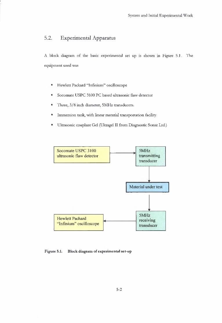
System and Initial Experimental Work
5.2. Experimental Apparatus
A block diagram o f the basic experimental set up is shown in Figure 5.1. The
equipment used was
• Hewlett Packard " I n f i n i u m " oscilloscope
• Socomate USPC 3100 PC based ultrasonic flaw detector
• Three, 3/8 inch diameter, 5MHz transducers.
• Immersion tank, wi th linear material transportation facility.
• Ultrasonic couplant Gel (Ultragel I I f r o m Diagnostic Sonar Ltd.)
Socomate USPC 3100 ultrasonic flaw detector
5MHz transmitting transducer
Hewlett Pachard "Infinium" oscilloscope
Material under test
5MHz receiving transducer
Figure 5.1. Block diagram of experimental set-up
5-2

System and Initial Experimental Work
5.2.1. Hewlett Packard "Infinium" Oscilloscope
The 54820A Inf in ium is a 2-channel oscilloscope (Figure 5.2.), wi th a Windows-based
graphical interface, and an integrated 3.5"floppy disc drive for data transfer. The
oscilloscope has a bandwidth o f 500 M H z , and the capability o f simultaneously
sampling, on both channels, at a rate o f 2 x 10⁹ sample/seconds. For consistency,
signal stability and to improve the signal to noise ratio the acquisition filter was set to
average the signal over 16 samples. The averaging stabilised the received signal on the
display screen, which facilitates accurate interpretation o f the signal. The 16 averages
was the opt imum setting for the signal acquisition on the oscilloscope, as a greater
numerical average would affect the refresh rate and sample length at the chosen
sampling frequency o f 50MHz. The sampling frequency o f 50MHz is outside the
Nyquist sampling frequency avoiding signal aliasing problems [1].
The pulse repetition frequency o f 5kHz, the systems slowest repeat rate, was applied to
facilitate signal decay and reduce spurious echoes. These parameters are applicable for
the duration o f the project unless otherwise stated.
- ^ = = • j .
•
1 HSOQMTE •
•» e «• *.. •'• c
Figure 5.2. H P Inf in ium oscilloscope. Figure 5.3. Socomate USPC3100.
5-3
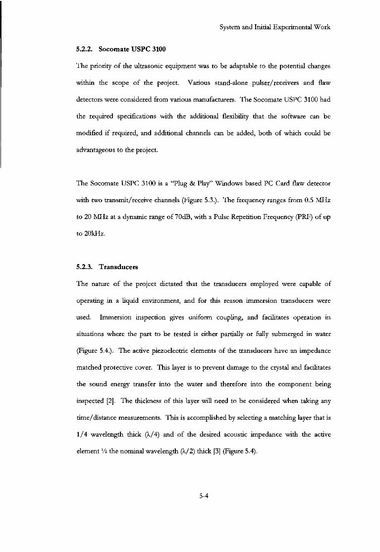
System and Initial Experimental Work
5.2.2. Socomate U S P C 3100
The priority o f the ultrasonic equipment was to be adaptable to the potential changes
within the scope o f the project. Various stand-alone pulser/receivers and flaw
detectors were considered f r o m various manufacturers. The Socomate USPC 3100 had
the required specifications wi th the additional flexibility that the software can be
modified i f required, and additional channels can be added, both o f which could be
advantageous to the project.
The Socomate USPC 3100 is a "Plug & Play" Windows based PC Card flaw detector
wi th two transmit/receive channels (Figure 5.3.). The frequency ranges f r o m 0.5 M H z
to 20 M H z at a dynamic range o f 70dB, with a Pulse Repetition Frequency (PRF) o f up
to 20kHz.
5.2.3. Transducers
The nature o f the project dictated that the transducers employed were capable o f
operating in a liquid environment, and for this reason immersion transducers were
used. Immersion inspection gives uni form coupling, and facilitates operation in
situations where the part to be tested is either partially or fully submerged in water
(Figure 5.4.). The active piezoelectric elements o f the transducers have an impedance
matched protective cover. This layer is to prevent damage to the crystal and facilitates
the sound energy transfer into the water and therefore into the component being
inspected [2]. The thickness o f this layer wi l l need to be considered when taking any
time/distance measurements. This is accomplished by selecting a matching layer that is
1/4 wavelength thick and o f the desired acoustic impedance with the active
element V* the nominal wavelength (X/2) thick [3] (Figure 5.4).
5-4
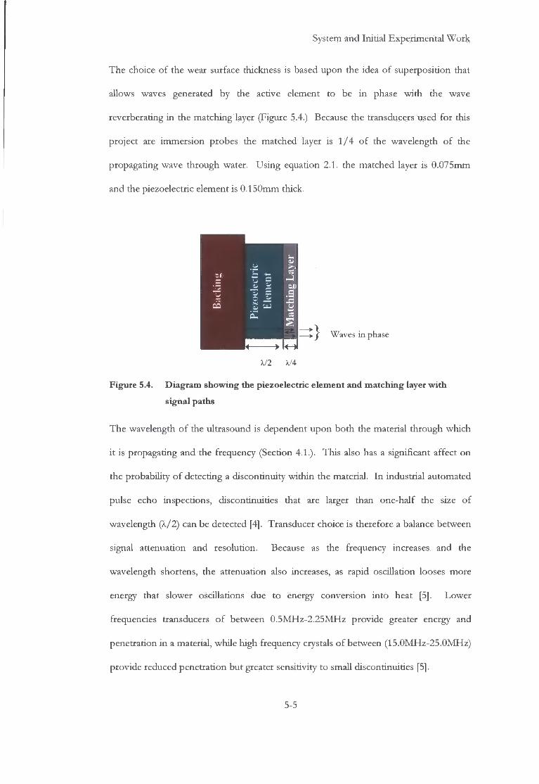
System and Initial Experimental Work
The choice o f the wear surface thickness is based upon the idea o f superposition that
allows waves generated by the active element to be in phase wi th the wave
reverberating in the matching layer (Figure 5.4.) Because the transducers used for this
project are immersion probes the matched layer is 1/4 o f the wavelength o f the
propagating wave through water. Using equation 2.1. the matched layer is 0.075mm
and the piezoelectric element is 0.150mm thick.
Figure 5.4. Diagram showing the piezoelectric element and matching layer wi th
signal paths
The wavelength o f the ultrasound is dependent upon both the material through which
i t is propagating and the frequency (Section 4.1.). This also has a significant affect on
the probability o f detecting a discontinuity within the material. I n industrial automated
pulse echo inspections, discontinuities that are larger than one-half the size o f
wavelength (k/2) can be detected [4]. Transducer choice is therefore a balance between
signal attenuation and resolution. Because as the frequency increases and the
wavelength shortens, the attenuation also increases, as rapid oscillation looses more
energy that slower oscillations due to energy conversion into heat [5]. Lower
frequencies transducers o f between 0.5MHz-2.25MHz provide greater energy and
penetration in a material, while high frequency crystals o f between (15.0MHz-25.0MHz)
provide reduced penetration but greater sensitivity to small discontinuities [5].
•=:} Waves in phase
X 4
5-5

System and Initial Experimental Work
The 5MHz piezoelectric transducers were chosen as the opt imum frequency for this project [6]. The transducers used during all these experiments were manufactured by N D T Systems and are 5MHz, immersion transducers, wi th a 0.375inch (9.525mm) diameter piezoelectric crystal (Figure 5.5.)
Figure 5.5. A typical ultrasonic immersion transducer
5.2.4. Transducer/Sample Coupling
Because o f the large impedance mismatch between air and in the case o f this project,
steel, water is commonly used for ultrasonic coupling [7]. Acoustic impedance is
discussed in section 4.11 o f this thesis. Water as a coupling medium is predominantly
used in automatic testing similar to the system under evaluation. The advantages o f
using this type o f testing are that the surface o f the material does not have to be
smooth as is required by contact testing. Water coupling also alleviates the possibility
that the transducers wi l l be struck by moving bar, and remove the complications
involved with the near field o f the probe. Ultrasonic sound waves travel at a much
lower velocity in water than in steel.
The longitudinal wave velocity is approximately four times greater in steel than in water.
Because o f the difference in the wave velocity, the length o f the near field is
proportionately greater in water [5].
5-6
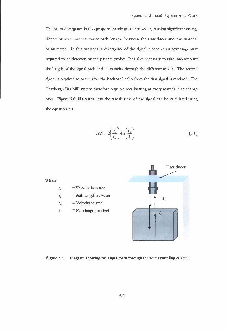
System and Initial Experimental Work
The beam divergence is also proportionately greater in water, causing significant energy dispersion over modest water path lengths between the transducer and the material being tested. In this project the divergence of the signal is seen as an advantage as it required to be detected by the passive probes. It is also necessary to take into account the length of the signal path and its velocity through the different media. The second signal is required to occur after the back-wall echo from the first signal is received. The Thrybergh Bar Mill system therefore requires recalibrating at every material size change over. Figure 5.6. illustrates how the transit time of the signal can be calculated using the equation 5.1.
ToF = 2 \K J
+ 2 [5.1.]
Transducer
Where
4
I.
— Velocity in water
= Path length in water
= Velocity in steel
= Path length in steel
Figure 5.6. Diagram showing the signal path through the water coupling & steel.
5-7
System and Initial Experimental Work
An ultrasonic couplant is used in virtually all contact testing applications, facilitating the transmission of ultrasonic sound energy between the transducer and the test piece. Where contact to the test piece is required a contact couplant, typically a viscous, nontoxic liquids, gels, or pastes will be used. Their use is necessary because sound energy, at the ultrasonic frequencies typically used for non-destructive testing, is not effectively transmitted through air because of the impedance mismatch [6]. Even extremely thin air gaps between the transducer and the test piece affect the efficiency of sound energy transmission and render testing impossible. Air interfaces represent a severe acoustic impedance mismatch with respect to both transducer and the material undergoing examination (Chapter 4.11.) The general purpose propylene glycol (CjHgO^ based couplant used in these experiments was chosen because it has good surface wetting properties, it will not corrode or otherwise attack materials, and it is easily washed off with water. It is also chemically non-reactive and does not evaporate quickly at room temperature. Propylene glycol has an acoustic impedance of 1.61 x 10s kgm'V1 and is
similar to that of water of1.48 x 105 kgm V.
5.3. Characterisation of the System
This section describes tests, which were carried out to characterise the response of the
measurement system to assist with the interpretation of experiments on different
sample materials. The output voltage from the U S P C 3100 flaw detector is a short
voltage pulse whose width can be modified to match half the wavelength of the
piezoelectric transducer to be excited and has been designed to drive transducers in the
0.5MHz to 20MHz range. Two tests were carried out, the first being to assess the
excitation voltage as a function of pulse width and the second to assess the received
voltage of a through transmission transmitter/receiver system coupled by water with no
sample present with respect to pulse width.
5-8

System and Initial Experimental Work
5.3.1. Transmitter Voltage
This experiment was set up to determine the variability in the transmitter voltage as a
function of pulse width. The test circuit was set up as shown in Figure 5.7. The pulse
width was swept through settings used to drive transducers from 0.5MHz to 20MHz.
The open circuit voltage was recorded through a 50Q impedance matched, 100 times
voltage attenuator, by the 500MHz bandwidth oscilloscope. The attenuator was
necessary as the voltage pulse was outside the safe operating range of the oscilloscope.
For each pulse width, the outputs from several pulses were taken and the average
maximum and minimum values were recorded, with the results are shown in Figure 5.8.
Socomate U S P C 3100
Pulser/Receiver
Socomate U S P C 3100
Pulser/Receiver Generated Voltage
Socomate U S P C 3100
Pulser/Receiver
"Infinium" oscilloscope Attenuated Voltage Pulse
Voltage
Attenuator
Figure 5.7. Block diagram showing flaw detector connected to the oscilloscope via
the inline lOOx signal attenuator
Since the transducer geometry determines the ultrasonic frequency, the ultrasonic
amplitude is dependent on the amount of excitation power present at that frequency.
The spectrum of a pulse is a sine cardinal (sine) function whose zeros are determined
by the pulse width. Figure. 5.8. shows the sine function characteristic effectively
traversing the ultrasonic frequency as the pulse width increases.
5-9

System and Initial Experimental Work
700
650
2- 600 Q.
> 550
t 500 <D
450 ° > 400
350
300
• • • • • . • • • •
Operating frequency * " •
/ : y • • • * • • . •
• • • • •
• • Input Max • Input Min • • Input Max • Input Min
• • • • • - -"-1 1 1 1—1
• • • — i — i — i — i — i — i — i — i — i — i — i — i — i — i — i — 0 1 2 3 4 5 6 7 8 9 10 11 12 13 14 15 16 17 18 19 20 21
Frequency (MHz)
Figure 5.8. Graph showing input voltage plotted against frequency
The results of these experiments showed that the excitation voltage is constant for
settings used to drive transducers up to 6.5MH2 where the voltage rapidly increased
(Figure5.8.). The area, at which the voltage started to increase, is above the designated
5MHz operating point for this project and was not investigated further. At any one
pulse width, the voltage was stable to within 6.7% as defined by three standard
deviations.
5.3.2. Receiver Characteristics
The aim of this experiment was to characterise a transmitter receiver system without a
sample present using water coupling to give a base measurement for comparison. This
was carried out in a temperature controlled immersion tank. The temperature of the
water was set at 24 + / - 1 degrees Celsius.
5-10
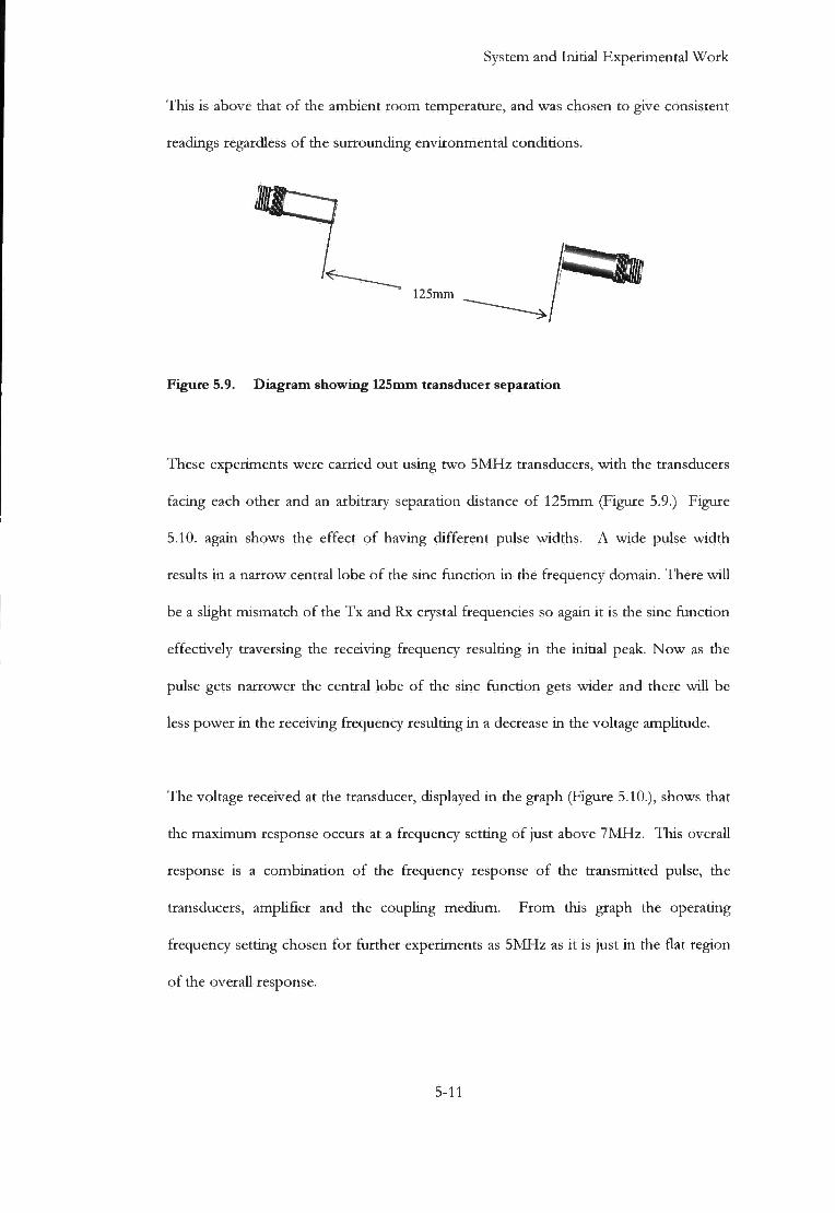
System and Initial Experimental Work
This is above that of the ambient room temperature, and was chosen to give consistent
readings regardless of the surrounding environmental conditions.
Figure 5.9. Diagram showing 125mm transducer separation
These experiments were carried out using two 5MHz transducers, with the transducers
facing each other and an arbitrary separation distance of 125mm (Figure 5.9.) Figure
5.10. again shows the effect of having different pulse widths. A wide pulse width
results in a narrow central lobe of the sine function in the frequency domain. There will
be a slight mismatch of the Tx and Rx crystal frequencies so again it is the sine function
effectively traversing the receiving frequency resulting in the initial peak. Now as the
pulse gets narrower the central lobe of the sine function gets wider and there will be
less power in the receiving frequency resulting in a decrease in the voltage amplitude.
The voltage received at the transducer, displayed in the graph (Figure 5.10.), shows that
the maximum response occurs at a frequency setting of just above 7MHz. This overall
response is a combination of the frequency response of the transmitted pulse, the
transducers, amplifier and the coupling medium. From this graph the operating
frequency setting chosen for further experiments as 5MHz as it is just in the flat region
of the overall response.
/ 125mm
5-11

System and Initial Experimental Work
* • : • 1 1 • • * • •
• • • • • Received Max
* • * i a • Received Min •
• •
• •
• Operating frequency •
•
• * • •
• #
• • •
0 1 2 3 4 5 6 7 8 9 10 11 12 13 14 15 16 17 18 19 20 21 Frequency (MHz)
Figure 5.10. Plot of received voltage through 125mm water separation
5.4. Initial experiments to assess the use of a single ttransmitter-multi-receiver system
The first sets of experiments were carried out on a steel billet to assess whether signals
could be detected from a receiving probe array. However, before this could be done,
the billet required characterisation using traditional pulse/echo techniques to determine
the type of defects present.
5.4.1. Characterisation of Billet
The billet was examined using a single transmitter/receiver probe placed directly on the
steel billet via a water based coupling gel. This resulted in the possibility of defects
within the near-field not being detected due to pressure wave rrtinima.
5-12

System and Initial Experimental Work
To overcome this, the orientation of the billet was changed to give complete coverage. To ensure that only the compression wave mode was evaluated, only the signal prior to the back-wall echo was used in these experiments, as other, slower modes, may have added additional complexity and will not be supported by the immersion system.
100
80 1 s t Back
60 wall & :ho
40 2 n d Back-wall :cho
20
n 3 _°_
n. -20
40
-60
-SO
-100 10 15 20 25 30 35 40 45
Time us
Figure 5.11. Scan of defect free section of billet showing 1st and 2 n d back-wall echoes
50
A clean back-wall echo signal, one with no detectable defect, was established in a
section of the material (Figure 5.11.). The compression wave velocity was then
measured using the time of flight for the first and 2 n d echo from the back-wall [8]. This
was used to calculate wave velocity together with the measured material thickness as
stated in BS EN 1223:2000, using Equation 5.2.
Distance Velocity
= Transit Time [5.2.]
5-13
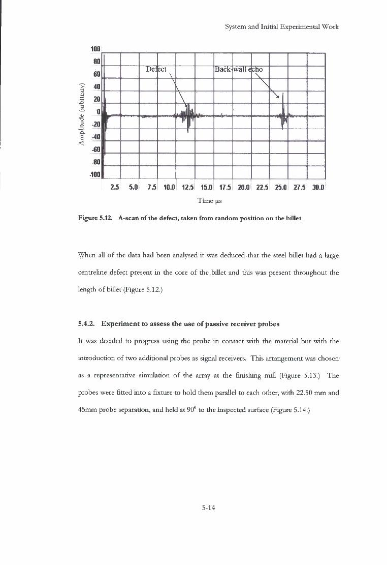
System and Initial Experimental Work
100
Be: set
4
Back" wall qcho
1 2.5 5.0 7.5 10.0 12.5 15.0 17.5 20.0 22.5 25.0 27.5 30.0
Time (is
Figure 5.12. A-scan of the defect, taken from random position on the billet
When all of the data had been analysed it was deduced that the steel billet had a large
centreline defect present in the core of the billet and this was present throughout the
length of billet (Figure 5.12.)
5.4.2. Experiment to assess the use of passive receiver probes
It was decided to progress using the probe in contact with the material but with the
introduction of two additional probes as signal receivers. This arrangement was chosen
as a representative simulation of the array at the finishing mill (Figure 5.13.) The
probes were fitted into a fixture to hold them parallel to each other, with 22.50 mm and
45mm probe separation, and held at 90° to the inspected surface (Figure 5.14.)
5-14

System and Initial Experimental Work
Figure 5.13. Representation of the transducer array at the finishing mill
The signal path lengths were calculated from the centreline of the transducers, with the
transmitting signal propagating at normal incidence to the probe face, and with the
reflected signal angle calculated away from the normal incidence.
45.0mm )-
22.5mm - _i
70.5mm
11
Figure 5.14. Experimental set-up showing transducer separation & signal paths
5-15

System and Initial Experimental Work
The procedure was to transmit using one probe (TX). This was connected to the pulser-receiver of the U S P C 3100. The other two probes were connected to the oscilloscope and operated as passive receivers (RX). It was established that the receiver probes RX1 and R X 2 , electro-magnetically detected the initial pulse emitted from the transmitting probe. The USPC 3100 has a trigger facility, however during these initial experiments the initial pulse proved a reliable trigger source and was subsequently utilized as the triggering signal for the oscilloscope. According to Brooks (2003) "There is nothing inherendy good or bad about electromagnetic coupling. Whether the consequences of this coupling are beneficial or not depends entirely on the circumstances" [9].
It was considered that when the transmitting probe received a reflected pulse then the
neighbouring probes might also detect these via the electromagnetic coupling. This
was not the situation however, as the timings would be almost identical for all of the
probes within the system and was calculated as approximately 7.5ps over the separation
distance of 22.50mm. This was calculated using the relationship stated in Equation 5.1.
and the electromagnetic velocity as 299 793 + / - 0.3 km/s [10]. As this was not the
case, the mechanism was discounted and the time of flight of the electro-magnetic
signal was deemed negligible and subsequently ignored.
Table 5.1 Signal Path lengths and Angles
Transducers Signal Path Lengths
(mm) + / - 0.01mm
Velocity
+ / - 50m/s
Angle of
Signal Paths
T i m e (us)
+ / - 0.01 us
T X - T X 70.50 + 70.50 = 141.00 5900 m/s 0.0° 23.90
T X - R X 1 70.50 + 74.00 = 144.50 5900 m/s 17.7° 24.50
T X - R X 2 70.50 + 83.64 = 154.14 5900 m/s 32.5° 26.13
5-16

System and Initial Experimental Work
The three-probe array scanned the billet in a similar raster scan pattern as the single pulse/echo probe. The geometry of the array was drawn out to measure the timings of the received signals and to compare with the signals received at the flaw detector (Table 5.1.)
1.2E-02 T
I 8.0E-03
Surface Wave
4.0E-03
0.0E+00
-4.0E-03
SSL Wave a <J -8.0E-03
-1.2E-02 J > 0 2 4 6 8 10 12 14 16 18 20 22 24 26 28 30
Time (us)
Figure 5.15. Signal received from transducer RX1
The received data from the passive receivers was captured using the oscilloscope and
analysed (Figure 5.15 and 5.16). The scans consistendy showed a low frequency high
amplitude signal and a low frequency low amplitude signal arriving prior to the back
wall echo. The high amplitude signal was evaluated through probe positioning and
signal timings as a surface wave reflecting from the vertical walls of the block (Equation
5.3.). Surface waves (SW) propagate at a velocity of 0.92x shearwave velocity within the
subject material [5], therefore the signal echoing from the sidewall travels a maximum
of 25mm from the centre of the probe to the sidewall, with shearwave velocity of
3240ms[ll].
5-17
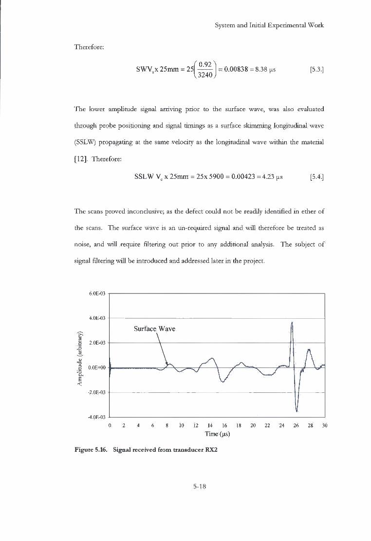
System and Initial Experimental Work
Therefore:
0.92^ SWV.x 25mm
13240 = 0.00838 = 8.38 us [5.3.]
The lower amplitude signal arriving prior to the surface wave, was also evaluated
through probe positioning and signal timings as a surface sltimming longitudinal wave
(SSLW) propagating at the same velocity as the longitudinal wave within the material
[12]. Therefore:
SSLW V c x 25mm = 25x 5900 = 0.00423 = 4.23 us [5.4.]
The scans proved inconclusive; as the defect could not be readily identified in ether of
the scans. The surface wave is an un-required signal and will therefore be treated as
noise, and will require filtering out prior to any additional analysis. The subject of
signal filtering will be introduced and addressed later in the project.
6.0E-03
4.0E-03
? ti 2.0E-03
I •8
f -2.0E-03
-4.0E-03
Surface Wave
\ V ^ . . A
\ II 0 2 4 6 8 10 12 14 16 18 20 22 24 26 28 30
Time (us)
Figure 5.16. Signal received from transducer RX2
5-18

System and Initial Experimental Work
5.5. Further experiments to assess the use of passive receiver probes
5.5.1 Calibrated sample
As previously stated a billet of steel with known properties was required to eliminate as
many variables as possible. It was decided that a V I ultrasonic calibration block would
be suitable for this purpose. The V I calibration block is a certified defect free block of
steel of known quality and surface finish and because of its commonality throughout
the ultrasonic N D T community would be an aid to future experimental repeatability
[13]. The V I calibration block is manufactured to the following standards BS 2704:1978
D I N 54120 I IW (International Institute of Welding). It is machined from normalized
low/medium carbon ferrite steel, to produce a fine homogeneous grain structure and
has dimensional tolerances of + 0.1 mm for the 25mm x 100mm x 300mm V I (Figure
5.17.) Velocity tolerances are stated in the following standard, (EN 12223:2000) and
declared 5920 ± 30 m/s for longitudinal waves. The specification states that it should
be machined with a surface finish (RJ value not greater than 0.8um [13]. Surface
roughness is rated as the arithmetic average deviation of the material surface valleys
and peaks [14].
300mm
50mm Diameter 100mm radius
V 15mm
Figure 5.17. V I ultrasonic calibration block
5-19
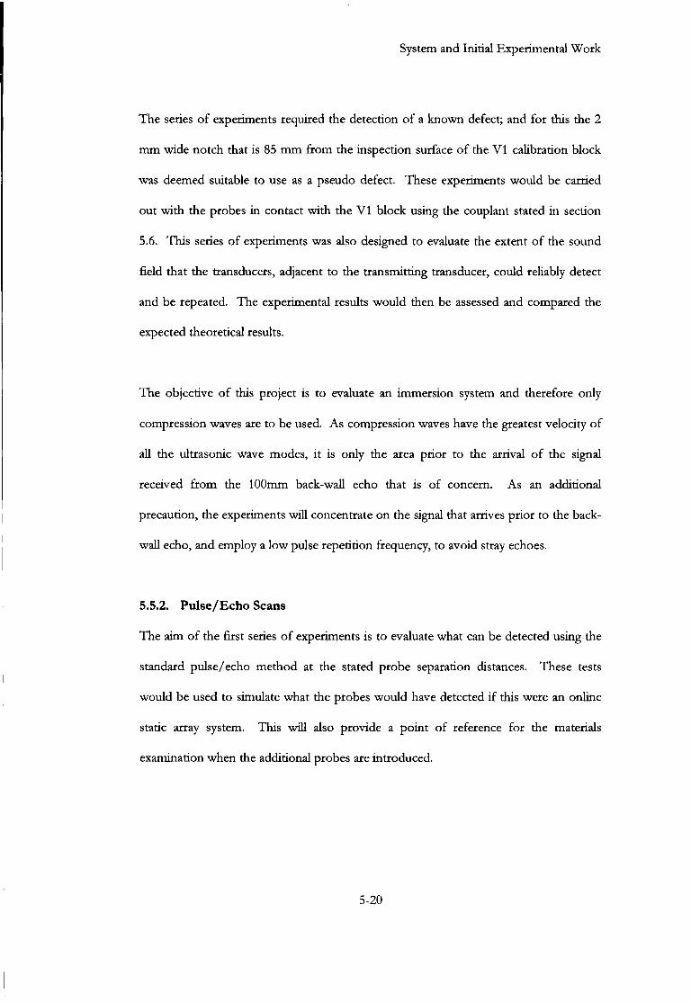
System and Initial Experimental Work
The series of experiments required the detection of a known defect; and for this the 2 mm wide notch that is 85 mm from the inspection surface of the V I calibration block was deemed suitable to use as a pseudo defect. These experiments would be carried out with the probes in contact with the V I block using the couplant stated in section 5.6. This series of experiments was also designed to evaluate the extent of the sound field that the transducers, adjacent to the transmitting transducer, could reliably detect and be repeated. The experimental results would then be assessed and compared the expected theoretical results.
The objective of this project is to evaluate an immersion system and therefore only
compression waves are to be used. As compression waves have the greatest velocity of
all the ultrasonic wave modes, it is only the area prior to the arrival of the signal
received from the 100mm back-wall echo that is of concern. As an additional
precaution, the experiments will concentrate on the signal that arrives prior to the back-
wall echo, and employ a low pulse repetition frequency, to avoid stray echoes.
5.5.2. P u l s e / E c h o Scans
The aim of the first series of experiments is to evaluate what can be detected using the
standard pulse/echo method at the stated probe separation distances. These tests
would be used to simulate what the probes would have detected if this were an online
static array system. This will also provide a point of reference for the materials
examination when the additional probes are introduced.
5-20

System and Initial Experimental Work
22.5mm 22.5mm 100mm
Prooe 2
Probe 3 Probe 1
2mm
/ 2mm Notch (defect]
Figure 5.18. V I calibration block with the probes in position
It was first necessary to determine the ultrasonic velocity within the V I Calibration
block. This velocity was measured using a single probe in pulse/echo mode as
described by Webb and Wykes [15] and was calculated to be 5900ms"' + / - 2% [16].
Each probe sequentially tested the calibration block in pulse/echo mode. The probes
were positioned as shown in Figure 5.18. using the same 22.50 mm probe separation as
used in the previous experiments carried out on the section of steel billet.
The A-scans that these examinations produced are displayed in Figures 5.19. 5.20. and
5.21. Figure 5.19. is of the full A-scan from the initial pulse to an arbitrary time after
the back-wall echo, the remaining A-scans are of the back-wall echo and the portion of
the signal directly preceding the back-wall echo, as this is the area where the notch
would be displayed i f detected.
5-21
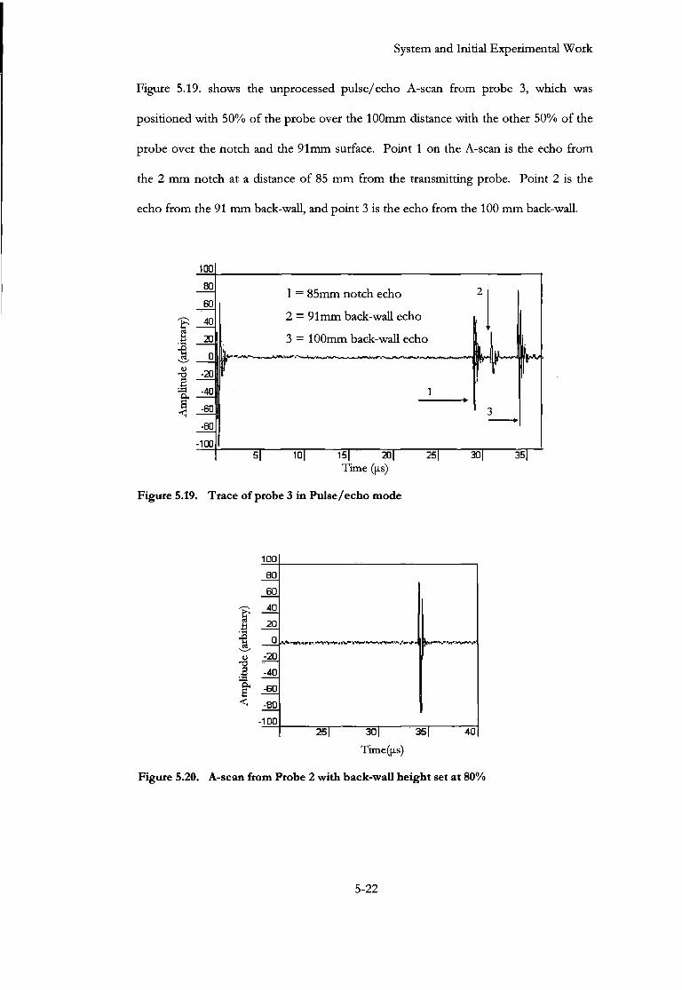
System and Initial Experimental Work
Figure 5.19. shows the unprocessed pulse/echo A-scan from probe 3, which was positioned with 50% of the probe over the 100mm distance with the other 50% of the probe over the notch and the 91mm surface. Point 1 on the A-scan is the echo from the 2 mm notch at a distance of 85 mm from the transmitting probe. Point 2 is the echo from the 91 mm back-wall, and point 3 is the echo from the 100 mm back-wall.
100 80 60 40 IT ^
.a _J°
M •5 -20" s — J -60
-80 -100
1 = 85mm notch echo
2 = 91mm back-wall echo
3 - 100mm back-wall echo
r
~S\ lOl 15| 20"! 25] 30] 35f Time ([xs)
Figure 5.19. Trace of probe 3 in Pulse/echo mode
? i
1 Cl4
1b~l ~3sT Time([xs)
Figure 5.20. A-scan from Probe 2 with back-wall height set at 80%
5-22
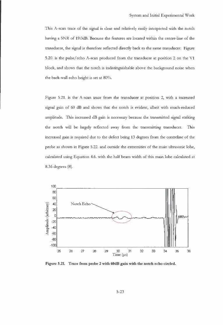
System and I n i t i a l Expe r i me n t a l W o r k
Th i s A-scan trace o f the signal is clear and relatively easily in te rpre ted w i t h the n o t c h hav ing a S N R o f 19.0dB. Because the features are located w i t h i n the centre-l ine o f the transducer, the signal is therefore ref lec ted direct ly back to the same transducer. F igure 5.20. is the pulse /echo A-scan p roduced f r o m the transducer at pos i t i on 2 o n the V I b lock , and shows that the n o t c h is indist inguishable above the background noise w h e n the back-wal l echo height is set at 8 0 % .
Figure 5 .21. is the A-scan trace f r o m the transducer at p o s i t i o n 2, w i t h a increased
signal gain o f 60 d B and shows that the n o t c h is evident, albeit w i t h much- reduced
ampl i tude . T h i s increased d B gain is necessary because the t ransmi t ted signal s t r ik ing
the n o t c h w i l l be largely ref lec ted away f r o m the t r ansmi t t ing transducer. T h i s
increased gain is required due to the defect be ing 13 degrees f r o m the centreline o f the
p robe as s h o w n i n Figure 5.22. and outside the extremities o f the m a i n ul trasonic lobe ,
calculated us ing E q u a t i o n 4.6. w i t h the h a l f beam w i d t h o f this m a i n lobe calculated at
8.36 degrees [8].
100
80
60
I 4 0
M 20 I A 0 u
1 - 2 0
% -40 | -60 -80
-100
Xotch F.cho
25 26 27 28 29 30 31 Time ((AS)
32 33 34 35 36
Figure 5.21. Trace from probe 2 with 60dB gain with the notch echo circled.
5-23

System and In i t i a l Expe r i me n t a l W o r k
Figure 5.22. Drawing showing 13° angle to the notch
Figure 5.23. shows the pu lse /echo A-scan f o r p robe 1 w i t h the back-wal l echo set at
8 0 % o f the screen height , and the defect is indist inguishable above the level o f the
noise. T h e centre o f p robe 1 is at a 24-degree angle f r o m the pseudo defect , as s h o w n
i n Figure 5.24.
25 | ~30T
Time ([is)
Figure 5.23. A-scan from Probe 1 with back-wall height set at 80%
5-24
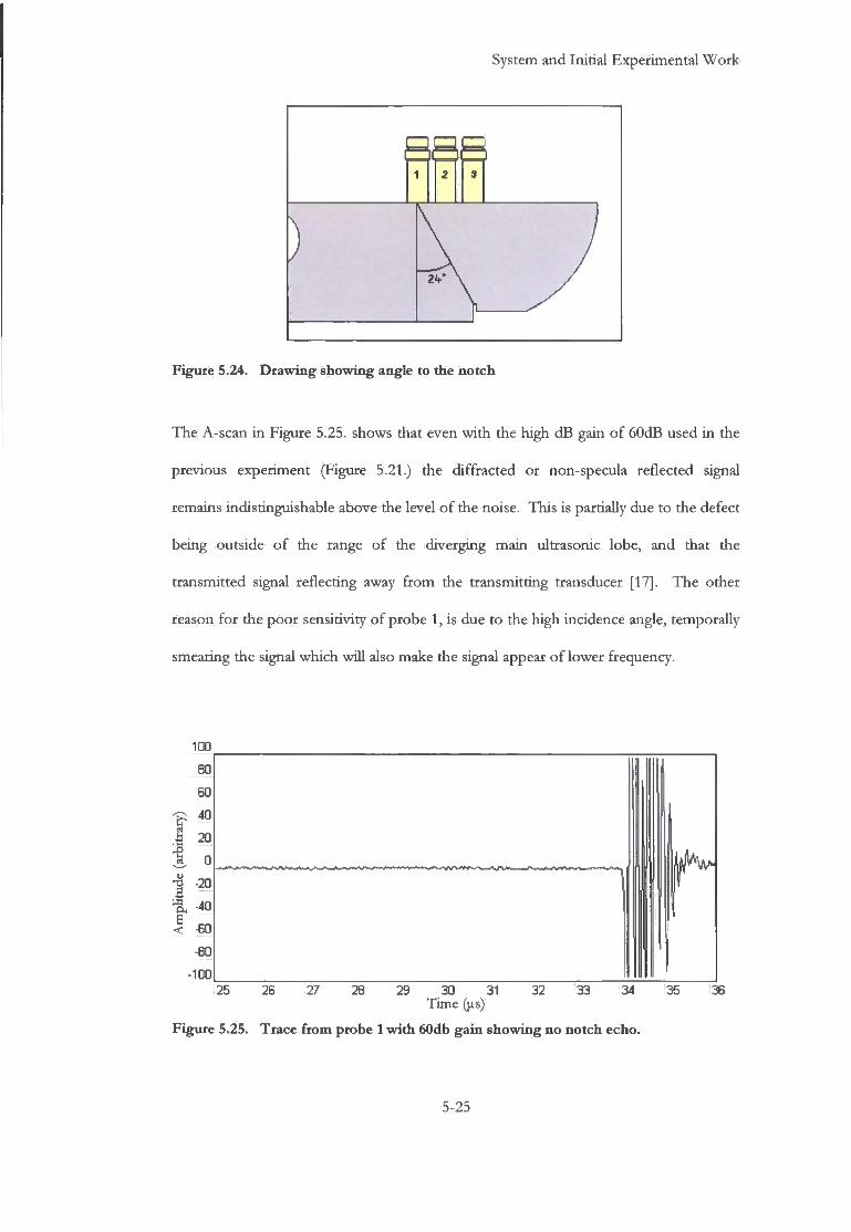
System and I n i t i a l Expe r imen t a l W o r k
F =)RR 1 2 9
)
Figure 5.24. Drawing showing angle to the notch
T h e A-scan i n Figure 5.25. shows that even w i t h the h i g h d B gain o f 60dB used i n the
previous exper iment (Figure 5.21.) the d i f f r a c t e d or non-specula re f lec ted signal
remains indis t inguishable above the level o f the noise. Th i s is part ial ly due to the defect
be ing outside o f the range o f the d iverg ing m a i n ultrasonic lobe , and that the
t ransmi t ted signal r e f l ec t ing away f r o m the t r ansmi t t i ng transducer [17] . T h e other
reason f o r the p o o r sensitivity o f p robe 1, is due to the h igh incidence angle, t empora l ly
smearing the signal w h i c h w i l l also make the signal appear o f l o w e r frequency.
100
80
60
40
a 20
-20
•40 e
< -60 IT!
100 25 26 27 28 29 30 31 32 33 34 35 36
Time (jis)
Figure 5.25. Trace from probe 1 with 60db gain showing no notch echo.
5-25

System and I n i t i a l Expe r imen ta l W o r k
5.6. Multi-Probe Scan
T h e m u l t i - p r o b e apparatus consists o f the three 5 M H z probes, placed i n a linear
arrangement w i t h a fixed separation distance o f 22.5 m m . T h e probes are at n o r m a l
incidence t o the upper surface o f a V I ca l ibra t ion b lock , as i n the previous pu lse /echo
exper iment (section 5.5.2.). Each p robe i n t u r n t ransmi t ted pulses, and the transit t ime
o f the r e tu rn ing pulses recorded. A s discussed i n the previously, the receiver probes
electro-magnetically detected the in i t i a l pulse emi t t ed f r o m the t ransmi t t ing probe , and
this was u t i l i sed as the t r igger ing signal f o r the oscil loscope [9] .
22.5mm 22.5mm
Probe 1 Probe 3
Probe 2
R
IS
• 100mm
2mm
Figure 5.26. V I calibration block showing signal paths and probe separation distances
5-26

System and Initial Experimental W o r k
T h e times between the transmitted and received signals were recorded, with a precision o f 0.05(xs, to determine the origin and path o f the received signal. Figure 5.26. shows the geometry o f the signal paths between the probes and the notch.
Table 5.2. displays these calculated times together with the calculated distances using
5900ms 4 for the speed o f sound in steel and the relationship in equation 5.5.
Distance Velocity
= Transit Time [5.5.]
Table 5.2. Calculated signal time and distances to the notch at 5900m/sec
A B C Backwall
Distance, mm + / - 0.05mm 95.60mm 87.50mm 85.00mm 100.00mm
Time, [AS +/-0.05 [*s (@ 5900ms"1) 16.20[is 14.80ns 14.40[is 16.95ns
Table 5.3. Probe to probe times and distances form the notch (taken from Table 5.2.)
Signal Paths
Theoretical
(Calculated from distances)
Actual
(from the A-scan graphs)
A + B 31.10[xs 30.95(is
A + C 30.60JAS 30.40jis
B + C 29.20[xs 29.20(is
5-27
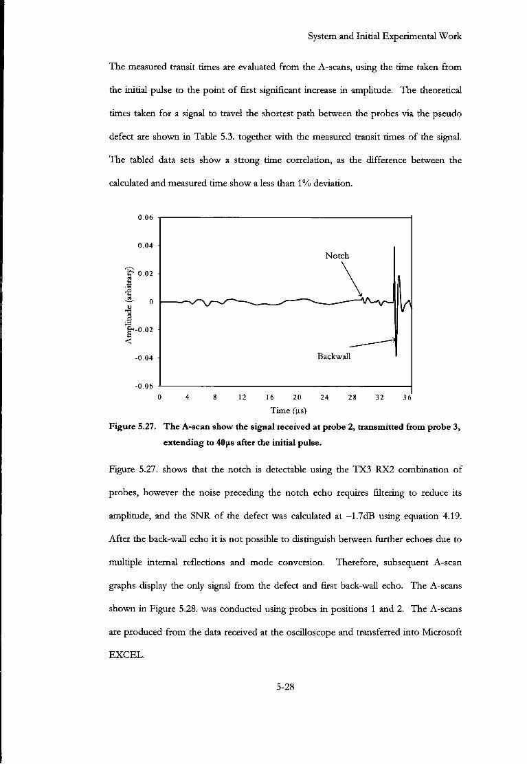
System and Initial Experimental W o r k
T h e measured transit times are evaluated from the A-scans , using the time taken from the initial pulse to the point o f first significant increase in amplitude. T h e theoretical times taken for a signal to travel the shortest path between the probes via the pseudo defect are shown in Table 5.3. together with the measured transit times o f the signal. T h e tabled data sets show a strong time correlation, as the difference between the calculated and measured time show a less than 1% deviation.
0.06
Notch
fr-0.02
Backwall
28 32 36 16 20 24
Time ("us)
Figure 5.27. The A-scan show the signal received at probe 2, transmitted from probe 3,
extending to 40(as after the initial pulse.
Figure 5.27. shows that the notch is detectable using the T X 3 R X 2 combination o f
probes, however the noise preceding the notch echo requires filtering to reduce its
amplitude, and the S N R o f the defect was calculated at - 1 . 7 d B using equation 4.19.
After the back-wall echo it is not possible to distinguish between further echoes due to
multiple internal reflections and mode conversion. Therefore, subsequent A-scan
graphs display the only signal from the defect and first back-wall echo. T h e A-scans
shown in Figure 5.28. was conducted using probes in positions 1 and 2. T h e A-scans
are produced from the data received at the oscilloscope and transferred into Microsoft
E X C E L .
5-28

System and I n i t i a l Expe r imen t a l W o r k
T h e probes were used as alternate t ransmit ter and receiver, however the displayed
signals are very similar. T h i s s imilar i ty is due to the signal paths be ing ident ical albeit i n
oppos ing direct ions. T h e mos t noticeable aspect o f the A-scans displayed i n Figure
5.28. is that the n o t c h , circled i n red , is v is ible cons ider ing the loca t ion o f the t w o
probes and there p o s i t i o n relative to the n o t c h . H o w e v e r i t w o u l d p r o v e to be d i f f i c u l t
t o automatical ly detect us ing signal th reshold ing techniques, due to the presence o f l o w
f requency noise and the ampl i tude o f the signal.
3.00E-02
2 00E-02
1.00E-02
| 00E+00
£ 1.00E-02 I
2.00E-02
-3.00E-02
-4.00E-02
Tx 1 Rx2 Tx 2 Rxl
25 27 29 31
Time (us)
33
Figure 5.28. T x 1 Rx2 and T x 2 R x l
35 37
T h e next stage o f the exper iment was conduc ted using the pair o f probes w i t h the
greatest p robe separation o f 4 5 m m . T h e n o t c h echo, c i rc led i n r ed , is easily vis ible
albeit a stretched and l o w e r ampl i tude signal due to the smearing e f f ec t because o f the
angle o f incidence.
5-29

System and I n i t i a l Expe r imen t a l W o r k
There is also a signal o f similar f requency, c i rc led i n green, f o l l o w i n g i t and preceding the back-wal l echo (Figures 5.29. and 5.30.) T h i s second signal was in i t i a l ly dismissed as an anomaly, however the exper iment was repeated numerous times and the second signal was a constant feature, and requi red invest igat ion.
0.015
0.010
0.005
« o.ooo -
0.005
0.010 -
-0.015 25 27 ">o n •»•» 35 37
Time ((is)
0.015
0.010 -
0.005
5 0.000
o 0.005
2 a 0.010
0.015
-0.020 25 27 ' 0 31 33 35 37
Time ([is)
Figure 5.29. T x - 3 Rx-1 Figure 5.30. T x - l R x - 3
a o.oo
-0.03 -
25 27 29 31 33 35
Time (us)
37
-0 -0.01 -
-0.04 25 27 29 31 33 35 37
Time (us)
Figure 5.31. T x - 2 Rx-3 Figure 5.32. T x - 3 Rx-2
5-30

System and Initial Experimental Work
Figures 5.31. and 5.32. show the A-scans for the probes in positions 2 and 3 on the V I calibration block. T h e signal from the notch is stronger and more readily identifiable as a 5 M H z signal than the previous series o f probe pairings. T h i s is due to the probes being both closer to the notch and that the notch lies closer to the centreline o f the main ultrasonic lobe.
T h e A-scans also indicate the presence the second echo signal and again it is similar in
frequency and amplitude as the notch echo signal. It was decided that this signal
required additional investigation, this was conducted using several different methods
and this is explained in the next section.
5.6.1 Spurious E c h o Investigation
Certain assumptions were made based upon the previous experimental results, in that
the ultrasonic wave was diffracting from the corner o f the notch. However there are
two signals present prior to the arrival of first back-wall echo. T h i s second signal is
present on all o f the experimental results from the V I calibration block that has the
notch signal, and this section sets out to investigate the source o f that second spurious
signal. Speculation as to the source o f the second signal gave four principle areas o f
investigation, these were:
1. E c h o from the 9 1 m m back-wall?
2. Mode converted echo from the near side o f the notch?
3. Creep wave f r o m the near side o f the notch traversing along the surface o f
the notch then diffracting from the far side?
4. Sidewall reflected echo after diffraction from the notch?
5-31
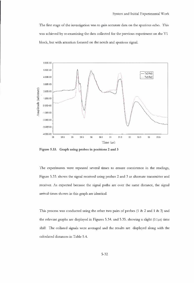
System and I n i t i a l Expe r imen ta l W o r k
T h e f i r s t stage o f the invest igat ion was to gain accurate data o n the spurious echo. T h i s was achieved b y re-examining the data col lected f o r the previous exper iment o n the V I b l o c k , bu t w i t h a t tent ion focused o n the n o t c h and spurious signal.
600E-03
5 00E-03
Tx2Rx3 Tx3Rx2 4.00E-03
3.00E-03
J 2.00E-03
a 1.00E-03
O.OOE+flC
0 -1.00E-03
2.00E-03
3.00E-03
-4.00E-03 1 1
28 28.5 29 29.5 30 30.5 31 31.5 32 32.5 33 33.5
Time (us)
Figure 5.33. G r a p h using probes in positions 2 and 3
T h e experiments were repeated several t imes t o ensure consistence i n the readings,
F igure 5.33. shows the signal received using probes 2 and 3 as alternate t ransmit ter and
receiver. A s expected because the signal paths are over the same distance, the signal
arr ival times s h o w n i n this graph are identical .
T h i s process was conduc ted using the other t w o pairs o f probes (1 & 2 and 1 & 3) and
the relevant graphs are displayed i n Figures 5.34. and 5.35. showing a sl ight (0.1 (is) time
s h i f t T h e col la ted signals were averaged and the results are displayed a long w i t h the
calculated distances i n Tab le 5.4.
5-32
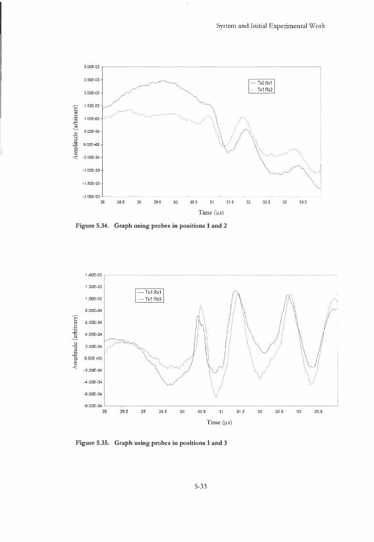
System and I n i t i a l Expe r imen ta l W o r k
3.00E-03
2.50E-03 Tx2 Rx1 Tx1 Rx2
2 OOE-03
1 S0E-03
1 .OOE-03
5 00E-04 u
•JA 0.00E+O0
B < -5 00E-M
J 1 OOE-03
1.50E-03
-2.00E-03 J
28 28.5 29 29.5 30 30.5 31 31.5 32 32.5 33 33.5
Time (us)
Figure 5.34. Graph using probes in positions 1 and 2
1 40E-03
1 20E-03 Tx3Rx1
1 OOE-03 Tx1 Rx3
f B 00E-04
6 00E-04
4.00E-04
2.00E-04
a 0.00E+O0 a
2.00E-04
-4 DOE-04
6OOE-04
-6.00E-04 1
28 28.5 29 29 5 30 30.5 31 31.5 32 32.5 33 33.5
Time (pis)
Figure 5.35. Graph using probes in positions 1 and 3
5-33

System and Initial Experimental Work
Table 5.4. Signal times and calculated distances fot second signal
Probe pairs T i m e us
+/-0 .05 us
Distance m m
+/-0.05 mm
2 & 3 31.30 184.67
1 & 2 33.00 194.70
1 & 3 32.40 191.16
A method was required to evaluate the signal transit distances recorded in Table 5.4.
and their possible paths. K u o et.al. (1998) describe several methods of using time
ellipses as a way of locating the tip o f surface breaking cracks [18]. Their method was
employed on surface breaking cracks on the inspected surface of the component,
however the method could be adapted for a crack in this case the notch, on the reverse
side of the component. T h e equations, 5.6. and 5.7., were used to calculate the ellipse
o f the spurious signal, with the ellipses being plotted against the V I calibration block in
Figure 5.36.
[5.6.]
Vertical Distance from Probe Centres =. Signal Distance ̂ ( Probe Separation
Signal Distance Horizontal Distance from Probe Centres =
[5.7.]
Probe Separation
5-34

System and I n i t i a l Expe r imen ta l W o r k
100mm Probes
//
Figure 5.36. Drawing of spurious signal ellipses plotted against the V I block
T h e ellipse test p r o v e d inconclus ive as t o the source o f the spurious signal, however i t
d i d el iminate the possibi l i ty o f the signal c o m i n g f r o m the 9 1 m m back-wal l . T h i s is
because the signal times are n o t l o n g enough and regardless o f w h i c h pair o f probes
was t r ansmi t t i ng or receiving, the signal w o u l d be speculatively ref lected away f r o m the
receiver. T h e t imings also show that the spurious echo signal cou ld n o t be a mode -
conver ted signal as the time calculat ion s h o w n i n Figure 5.36. and was conduc ted using
the pair o f probes that y ie ld the clearest signals, probes 2 and 3. T h e ve loc i ty o f the
transverse wave was taken as 3200 m/sec . i n steel [5] .
Table 5.5. Longitudinal and transverse wave transit times for signal paths C & B
Signal pa th distance taken
f r o m Figure 5.9.
( + / - 0.05mm)
L o n g i t u d i n a l wave
@ 5900 m/ sec
(+/-0.05 (is)
Transverse wave
@ 3200 m/ sec
(+/-0.05 (is)
(C.) 8 5 . 0 0 m m 14.40us 26.56us
(B.) 8 7 . 9 0 m m 14.90us 27.69us
5-35

System and I n i t i a l Expe r imen ta l W o r k
Transit time = C T + B L = 26.56 + 14.90 = 41.46us [5.8.]
Transit time = C L + B T — 14.40 + 27.69 = 42.09us [5.9.]
I t be seen f r o m the transit times calculated i n equations 5.8. and 5.9. the spurious signal
is n o t a l ong i tud ina l wave , m o d e conver ted at the n o t c h i n t o a transverse wave. T h e
time ellipses also show that the spurious echo is n o t a creep wave f r o m the near side o f
the n o t c h , t raversing a long the surface o f the n o t c h then d i f f r a c t i n g f r o m the far side to
a receiver. T h i s is because despite its name, a creep wave travels at the same veloc i ty as
its generating wave [6] , i n this case a compress ion wave. H o w e v e r a compress ion wave
requires 0.34(xs and a shear wave 0.63us to travel the 2 m m w i d t h o f no t ch . T h i s
a m o u n t o f time constitutes 1-2% o f the to ta l transit time and is w i t h i n the ant icipated
m a r g i n o f er ror and therefore addi t ional tests are required.
lW OJ
4mm notch
-<;< 6mm notch
10mm notch
Figure 5.37. L i n e drawing of the experimental set-up including the transducers in
position for examination of the 10mm notch
5-36
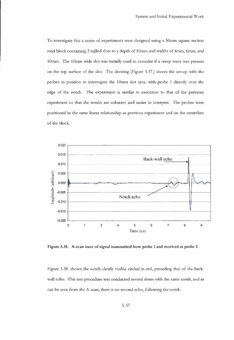
System and I n i t i a l Expe r imen ta l W o r k
T o investigate this a series o f experiments were designed us ing a 5 0 m m square section
steel b l o c k con ta in ing 3 m i l l e d slots to a dep th o f 1 0 m m and w i d t h s o f 4 m m , 6 m m , and
1 0 m m . T h e 1 0 m m w i d e slot was ini t ia l ly used to consider i f a creep wave was present
o n the t o p surface o f the slot. T h e d rawing (Figure 5.37.) shows the set-up w i t h the
probes i n p o s i t i o n to interrogate the 1 0 m m slot area, w i t h p robe 1 direct ly over the
edge o f the n o t c h . T h e exper iment is similar i n execut ion to that o f the previous
exper iment so that the results are coherent and easier to in terpre t . T h e probes were
pos i t ioned i n the same linear relat ionship as previous exper iment and o n the centreline
o f the b lock .
0.020 -I
0.015
0.010
1 0.005
0.000 u 1 -0.005 a
| -0.010
-0.015
-0.020
Back-wall echo
It - fT>
Notch echo ^
Time (pis)
Figure 5.38. A-scan trace of signal transmitted from probe 1 and received at probe 2
Figure 5.38. shows the n o t c h clearly vis ible c ircled i n red, preceding that o f the back-
w a l l echo. T h i s test procedure was conduc ted several times w i t h the same result , and as
can be seen f r o m the A-scan, there is n o second echo, f o l l o w i n g the no t ch .
5-37
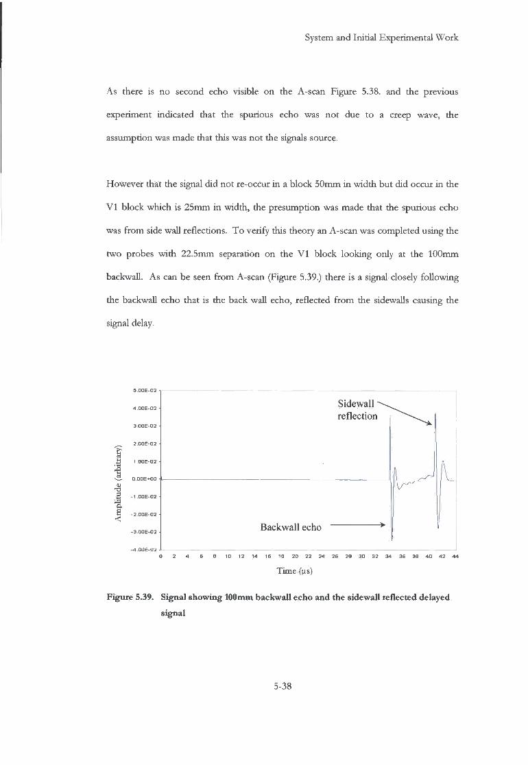
System and I n i t i a l Expe r imen ta l W o r k
A s there is n o second echo vis ible o n the A-scan Figure 5.38. and the previous
exper iment indica ted that the spurious echo was n o t due to a creep wave, the
assumpt ion was made that this was n o t the signals source.
H o w e v e r that the signal d i d n o t re-occur i n a b l o c k 5 0 m m i n w i d t h bu t d i d occur i n the
V I b l o c k w h i c h is 2 5 m m i n w i d t h , the p r e s u m p t i o n was made that the spurious echo
was f r o m side w a l l ref lect ions . T o v e r i f y this theory an A-scan was comple ted us ing the
t w o probes w i t h 2 2 . 5 m m separation o n the V I b l o c k l o o k i n g on ly at the 1 0 0 m m
backwal l . A s can be seen f r o m A-scan (Figure 5.39.) there is a signal closely f o l l o w i n g
the backwal l echo that is the back w a l l echo, ref lec ted f r o m the sidewalls causing the
signal delay.
2 0 0 E - 0 2 -
I a a <
O.DOE-rtJO - .
Sidewall reflection
Backwall echo
0 2 4 6 6 10 12 14 16 16 26 22 24 26 26 30 32 34 36 38 40 4 2 44
Time (us)
Figure 5.39. Signal showing 100mm backwall echo and the sidewall reflected delayed
signal
5-38

System and Initial Experimental Work
5.7. Conclusion
The measurement system was characterised and suitable operating conditions were
chosen, resulting in 5MH2 frequency setting being employed for the duration of this
project.
The test on the steel billet had proved inconclusive due partly to the fact that the defect
was large and obscured the back-wall echo signal. It was suggested that the project
progressed to an immersion test on the billet, with the additional probes in position.
However it was decided that it was premature to move the project in this direction at
this stage, as it added additional variables to the experiment. Because of the potential
confusing signal traces, it was decided to eliminate as many of the variables as possible.
The subsequent series of experiments was carried out on a subject containing a simple
known target. The options considered included a section of billet with a flat-bottomed
hole, as the target defect, as this method is widely employed within the N D T industry
[6]. However as the quality of the material could not be assured, it was decided to use a
V I calibration block, as the steel was of certified quality (BS 2704:1978). The 2mm
notch could be utilized as a pseudo defect, and as this was a standard calibration tool, it
would aid repeatability.
The next section of the Chapter was initiated to evaluate the potential within the probe
array to reliably detect a known defect. For this the 2mm wide notch that is 85mm
from the inspection surface of the V I calibration block was used as a pseudo defect.
5-39

System and Initial Experimental Work
The aim of this series of experiments was to evaluate what features within the V I block
the individual probes, while operating in standard pulse/echo configuration, could be
discerned. The experiment was simulating what the probes would detect i f this were an
online system and to provide a point of reference for future experiments.
The first set of experiments using the V I calibration block showed that the probe at
position 3, could detect the notch and the back-wall echoes from both the 91mm back-
wall and the 100mm back-wall. This was as expected because the probe was positioned
direcdy above these features and therefore able to receive the direcdy reflected signal.
That the probe in position 2 also picked up a returning signal from the 2mm notch
however was unexpected. At 13 degrees away from the centreline of maximum
intensity, the notch was outside of the stated theoretical extremities of the main
ultrasonic lobe. This could also account for the large increase in signal gain required to
detect the notch (Figure 5.21. and 5.25.). That the signal was detected and identified
requires some form of non-specular reflection, the probable method of which is
diffraction, as diffuse reflection requires a rough surface and the boundary variations to
be of the same order of magnitude or larger than the ultrasound wavelength being used
[19].
For the notch to be detected at the probe in position 2 using an automated system
would prove problematic to threshold the defect due to low signal to noise ratio. Also
operating at the required elevated levels of signal gain would lead to an increase in false
alarms.
5-40
System and Initial Experimental Work
Section 5.5.3. was concerned with the spurious second echo and set out to investigate
its source. This second signal was present on all of the experimental results from the
V I calibration block, and could not be ignored or dismissed as an anomaly. The
procedure to discover the signals source proved to be longer and more involved than
initially anticipated. However the evaluation showed that the signal was due to internal
reflections owing to the V I block being relatively narrow in profile and interacting with
the diverging ultrasonic beam.
The investigation into the spurious signal, introduced a technique devised by Kuo et. al.
(1998) [18] for measuring the depth of surface breaking cracks on the inspection
surface, using pairs of half ellipses. This half ellipse method was adapted for use on the
back surface of the V I block, and was used successfully to evaluate the source of the
echo. In the next chapter, the technique will be evaluated further and in detail.
This initial experimental work served to layout the path of the next series of
experiments. These experiments will be conducted using the experience and
understanding taken from this work, in that care must be taken as to the source of the
echo signal and the half ellipse technique can be employed for echolocation.
5-41

System and Initial Experimental Work
5.8. References:
1. Chen, C.-T., Digital Signal Processing; Spectral Computation <& Filter Design. 2001, New York, U.S.A.: Oxford University Press.
2. Soh, H.T., et al., Silicon micromachined ultrasonic immersion transducers. Journal of American Institute of Physics, 1996. 69(24): p. 3674-3676.
3. Ladabaum, I . , et al. Silicon Substrate Ringing in Microfabricated Ultrasonic Transducers. in IEEE Ultrasonics Symposuim. 2000. San Juan, Puerto Rico., p.943-946
4. Payne, P.A., Ultrasonic Transducers: Design, Construction and Applications. International Journal of Materials, 1994. 9: p. 403-427.
5. Krautkramer, J. and H. Krautkramer, Ultrasonic Testing of Materials. 1990, New York: Springer-Verlag. 677.
6. Birks, A.S. and R.E. Green Jr., Ultrasonic Testing. 2nd ed. Nondestructive Testing Handbook, ed. P. Mclntire. Vol. 7. 1991, Baltimore, Maryland, U.S.A.: American Society for Nondestructive Testing. 893.
7. Wolfram, A. Automated ultrasonic inspection, in 15th WCNDT conference. 2000. Rome, Italy: www.karldeutsch.de/PDF/Automated UT inspection May00.PDF.
8. Hellier, C.J., Handbook of Nondestructive Evaluation. 2001, New York, U.S.A.: McGraw-Hill.
9. Brooks, D., Signal Integrity Issues and Printed Circuit Board Design. 2003, New Jersey: Prentice Hall.
10. Kingsbury, R.F., Elements of Physics. 1965, Princeton, New Jersey, U.S.A.: D. Van Nostrand Co. Inc.
11. Halmshaw, R., Mathematics and Formulae in NDT. 2nd ed. 1993, Northampton: The British Institute of Non-Destructive Testing.
5-42

System and Initial Experimental Work
12. Sathish, S., et al., ljocal surface skimming longitudinal wave velocity and residual stress mapping. The Journal of the Acoustical Society of America, 2004.115(1): p. 165-171.
13. Markucic, D., et al. Quality Requirements for Ultrasonic Testing Calibration Blocks, in 8th ECNDT. 2003. Barcelona, Spain.
14. Pohanish, D . and C. McCauley, Machinery's Handbook Pocket Companion: A Reference Book for the Mechanical Engineer. 2000, New York, USA: Industrial Press Inc. 317.
15. Webb, P. and C. Wykes, Suppression of second-time-around echoes in high firing rate ultrasonic transducers. N D T & E International, 1995. 28(2): p. 89-93.
16. Kumar, Y. and A. Kumar. The Calibration of Ultrasonic Flaw Detectors, in NDE 2002 Indian Society for Non-Destructive Testing. 2002. Chennai (Madras), India.
17. Ben Amor, M., et al., Influence of attenuation on the behavior of refracted elastic waves at the interface between anisotropic media. Ultrasonics, 2002. 40: p. 561-565.
18. Kuo, M.K., et al., Locating the crack tip of a surface-breaking crack. Part I. Line crack. Ultrasonics, 1998. 36: p. 803-811.
19. Charlesworth, J.P. and J.A.G. Temple, Engineering Applications of Ultrasonic Time-of Flight Diffraction. Second Edition ed. Ultrasonic Inspection in Engineering, ed. M.J. Whitde. 2002, Baldock: Research Studies Press Ltd. 254.
5-43

Time Ellipse Defect Location
Chapter 6.
Time Ellipse Defect Location
6.1. Introduction
This chapter further explores the potential for using the ellipse method, introduced in
the previous chapter. In the previous chapter, the factors affecting the ellipse
technique were investigated. In this section, the technique will be evaluated as a tool for
locating the notch of the V I calibration block. This sample was chosen as the material
and propagation properties have already been characterised.
The method used during this series of experiments differs from the one utilised by Kuo
et.al. (1998) [1] who employed the technique for the location of nearside surface
breaking cracks. In their paper, the basic principle was to align the source and the
receivers geometrically on either side of the surface-breaking cracks, which is similar to
time-of-flight diffraction (TOED), whereas the probes in this experiment would be
positioned either above the defect or to one side of the defect.
6-1

Time Ellipse Defect Location
The ellipse scans would be conducted using the identical probe configuration as all of the previous experiments i.e. 22.5mm and 45mm. Charlesworth et.al. (2002) during their study of the ToFD technique, advocated the use of multi-probe scans and specifically the use of different probe separations as a method for ensuring reliable detection [5].
6.2. Ellipse Equations
An ellipse has two axes of symmetry, the Major axis 2a and the Minor axis 2,, [2]. In
this experiment, each transmitter receiver pair was considered as the twin foci of the
ellipse (Fi&cF2).
2
!
2c
2a
Major axis
Figure 6.1. Diagram of the ellipse dimensional relationships
6-2

Time Ellipse Defect Location
With the distance between the probes (2c) and half distance between the probe centres being the centre of the ellipse (C). The signal transit time between the probe pair of which has diffracted from the defect was considered as the radii (r,+ t^).
The following equations (Eq.6.1. and Eq.6.2.) provide the Minor and Major axis of the
ellipse.
Minor Axis
^ ! + r 2 V (2c [6.1.] V ^ )
Major Axis
2a = rx + r2 [6.2.]
6.3. Ellipse Calculations
As discussed in the previous chapter (Chapter 7.3.), the probes are at normal incidence
to the upper surface of a V I calibration block and each probe sequentially transmitted
pulses. The experiment was repeated several times and the average transit time of the
signal returning to the two passive probes was recorded. The sampling frequency
employed was 50MHz (20ns/point) to give accurate reproduction of the waveform [3].
This frequency was also sufficiendy above that of the signal frequency of 5MHz, to
avoid the problems of signal aliasing [4].
6-3

Time Ellipse Defect Location
Table 6.1. displays the average of recorded times together with the distances calculated using 5900 m/s for the speed of sound in steel and the relationship in Equation 5.3.
Table 6.1 Signal path distance calculated at 5900m/sec
Distance (mm) Time (|j.s)
Signal path +/-0.05mm +/-0.05(xs
A & B 182.60 30.95
A & C 179.40 30.40
B & C 172.30 29.20
The calculated signal path distances were substituted into the two ellipse equations
(Equation 6.1 and 6.2.) Using the dimensions calculated from the equations, ellipses
were drawn and plotted against a drawing of the V I calibration block.
Probes 1 and 2, signal path A-B.
Minor Axis 2 b = 2. 182.61 \ 2
f 22.5 Y v ^ J
[6.3.]
.\b = 90.61mm
MajorAxis2 a =91.30 + 91.30 = 182.60 [6.4.]
. . a = 91.30 mm
6-4
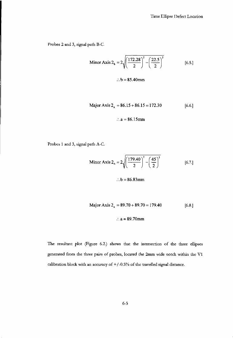
Time Ellipse Defect Location
Probes 2 and 3, signal path B-C.
Minor Axis 2 b = 2. f 172.28? (22.5^2
V ^ J [6.5.]
b = 85.40mm
Major Axis2 a =86.15 + 86.15 = 172.30 [6.6.]
a = 86.15mm
Probes 1 and 3, signal path A-C.
Minor Axis 2K = 2, 179.40 f 4 5 ?
v ^ J
[6.7.]
b = 86.83mm
Major Axis 2 a = 89.70 + 89.70 = 179.40 [6.8.]
.-. a = 89.70mm
The resultant plot (Figure 6.2.) shows that the intersection of the three ellipses
generated from the three pairs of probes, located the 2mm wide notch within the V I
calibration block with an accuracy of +/-0.5% of the travelled signal distance.
6-5

Time Ellipse Defect Location
Probe8 Ellip
[ 1
<
\
\ Figure 6.2. Drawing of ellipses plotted against the V I block, showing signal paths
6.4. Conclusion
The first section of this chapter investigated the half ellipses as a geometric method of
accurately locating a defect. Kuo et.al. (1998) had successfully employed the technique
to size surface breaking cracks. The experimental work conducted using the ellipse
method of geometric location described in this chapter shows that the technique was
successfully adapted the to locate the defect on the bottom surface of the V I
calibration block. The use of three probes and the combination of signal paths
provided data to locate the notch to an accuracy of +/-0.5%, using the intersection of
the three ellipses. However, the weaker echo signals required a subjective approach in
their time estimation. The next chapter will set out to address this problem with the
application of DSP techniques to the signals.
This work was presented at the 30 t h Annual Review of Progress in Quantitative Non
destructive Evaluation (QNDE) July 27-August 1, 2003, held in Green Bay, Wisconsin
U.S.A. Also a modified version of this work was published in the journal, Non
destructive Testing and Evaluation [6],
6-6
Time Ellipse Defect Location
References
Kuo, M.K., T.R. Lin, P.L. Liu, and T.T. Wu, Locating the crack tip of a surface-breaking crack. Parti. Line crack. Ultrasonics, 1998. 36: p. 803-811.
Stroud, K.A., Mathematics for Engineering Technicians. Vol. 2A, Practical Applications. 1981, Cheltenham, UK.: Stanley Thornes.
Fritsch, C, M. Parrilla, T. Sanchez, and O. Martinez, Beamforming with a reduced sampling rate. Ultrasonics, 2002. 40: p. 599-604.
Chen, C.-T., Digital Signal Processing. 2001, New York: Oxford University Press, Inc. 440.
Charlesworth, J.P. and J.A.G. Temple, Engineering Applications of Ultrasonic Time-of-Flight Diffraction. Second Edition ed. Ultrasonic Inspection in Engineering, ed. M.J. Whittle. 2002, Baldock: Research Studies Press Ltd. 254.
Snowdon, P.C., S. Johnstone, and S. Dewey, A 2D Static Ultrasonic Array of Passive Probes for Improved Probability of Detection. Nondestructive Testing And Evaluation, 2003.19(3): p. 111-120.
Signal Echo Enhancement using DSP
Chapter 7.
Signal Echo Enhancement using DSP
7.1. Introduction
This chapter sets out to investigate and subsequently employ the most suitable digital
signal filter to enhance the signal to noise ratio of the received ultrasonic signal. In
previous chapters, the signal returning from the notch has been preceded by low
frequency high amplitude noise. This has been identified using Equation 5.3. as a
surface wave reflecting from the sides of the test material. It is however an un-required
signal, and it will be treated as noise and filtered out, as this could cause problems with
automated defect detection systems that rely upon signal thresholding, which requires
the defect signal to be of greater amplitude than the ambient noise.
The MathWorks program, MATLAB®, is extensively used to apply several various
signal filters in order to improve the signal to noise ratio (SNR). To obtain these
results, the unprocessed signals were recorded using the digital oscilloscope with a
sampling rate of 50M samples/sec (50MHz) as stated in Chapter 5., and transferred via
Microsoft EXCEL digitally into MATLAB®.
7-1

Signal Echo Enhancement using DSP
The chapter will then progress and investigate the potential of combining the two techniques, that of ellipse geometry and the application of DSP to enhance the likelihood of detection of the defect within the V I calibration block.
7.2. Digital Signal Processing
The discontinuity signals measured by an ultrasonic N D T system; include the effects of
the measurement system, and are corrupted by different types of noise. According to
Kazanavicius et.al. (2003), an A-scan signal may carry information on material
properties and defects, but the information appears within, or together with, various
guises of noise [2]. There is a complex interaction between the defect geometry,
diffracted, mode converted waves and the back-scattered ultrasonic waves inside the
test piece.
Current means of automated defect detection use various preset level gates within the
flaw detector. The system is alerted when the amplitude level moves above or below
the set threshold of the gate and is defined as monitor level or thresholding [3]. Much
research has been done on ultrasonic signal processing, for more reliable and versatile
signal processing techniques without a definitive solution [4].
It was decided to conduct the initial DSP filtering using the signal with the best signal
to noise ratio (SNR) and with the most defined notch diffraction signal. The signals
from the previous ellipse experiment were collated and transferred into MATLAB®.
7-2
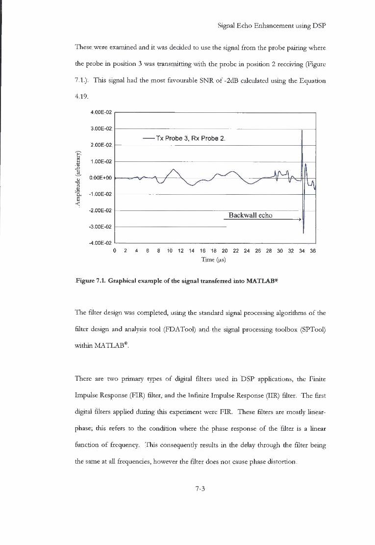
Signal Echo Enhancement using DSP
These were examined and it was decided to use the signal from the probe pairing where the probe in position 3 was transmitting with the probe in position 2 receiving (Figure 7.1.). This signal had the most favourable SNR of -2dB calculated using the Equation 4.19.
4.00E-02
3.00E-02
2.00E-02
f H 1.00E-02
i V 0.00E+00
1 O. -1.00E-02 a
<
-2.00E-02
-3.00E-02
-4.00E-02
Tx Probe 3, Rx Probe 2.
ft
Backwall echo
0 2 4 6 8 10 12 14 16 18 20 22 24 26 28 30 32 34 36
Time ([is)
Figure 7.1. Graphical example of the signal transferred into MATLAB®
The filter design was completed, using the standard signal processing algorithms of the
filter design and analysis tool (FDATool) and the signal processing toolbox (SPTool)
within MATLAB®.
There are two primary types of digital filters used in DSP applications, the Finite
Impulse Response (FIR) filter, and the Infinite Impulse Response (IIR) filter. The first
digital filters applied during this experiment were FIR. These filters are mosdy linear-
phase; this refers to the condition where the phase response of the filter is a linear
function of frequency. This consequendy results in the delay through the filter being
the same at all frequencies, however the filter does not cause phase distortion.
7-3
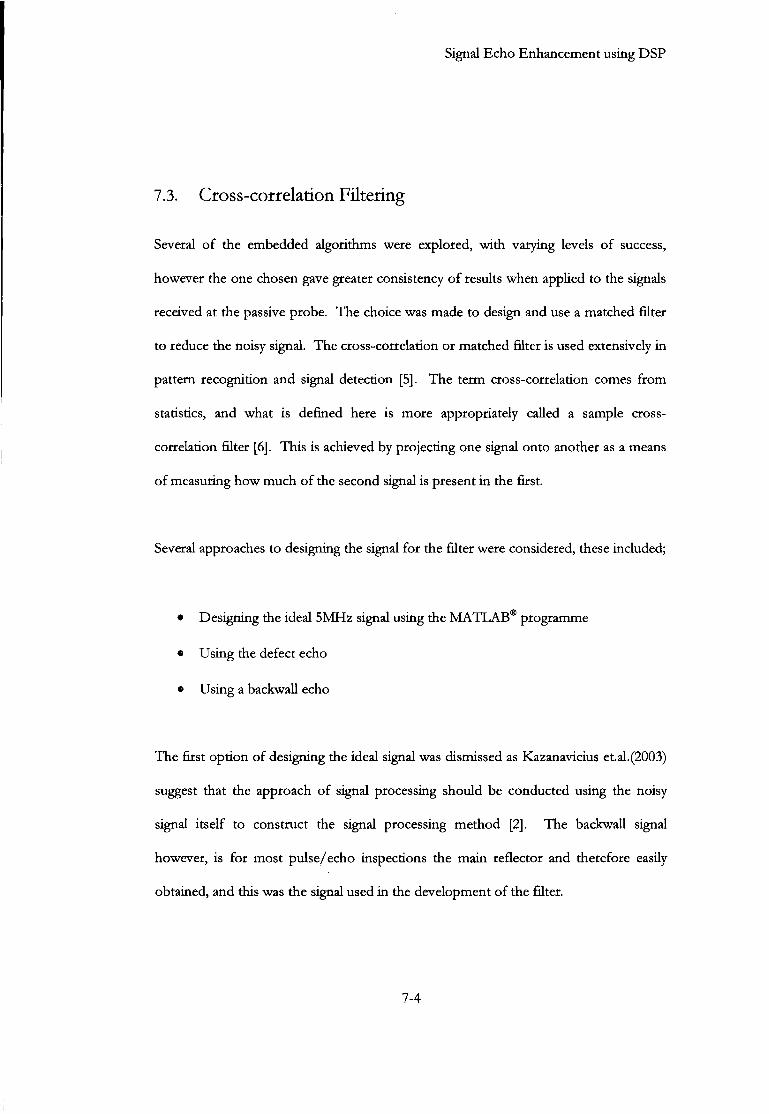
Signal Echo Enhancement using DSP
7.3. Cross-correlation Filtering
Several of the embedded algorithms were explored, with varying levels of success,
however the one chosen gave greater consistency of results when applied to the signals
received at the passive probe. The choice was made to design and use a matched filter
to reduce the noisy signal. The cross-correlation or matched filter is used extensively in
pattern recognition and signal detection [5]. The term cross-correlation comes from
statistics, and what is defined here is more appropriately called a sample cross-
correlation filter [6]. This is achieved by projecting one signal onto another as a means
of measuring how much of the second signal is present in the first.
Several approaches to designing the signal for the filter were considered, these included;
• Designing the ideal 5MHz signal using the MATLAB® programme
• Using the defect echo
• Using a backwall echo
The first option of designing the ideal signal was dismissed as Kazanavicius et.al.(2003)
suggest that the approach of signal processing should be conducted using the noisy
signal itself to construct the signal processing method [2]. The backwall signal
however, is for most pulse/echo inspections the main reflector and therefore easily
obtained, and this was the signal used in the development of the filter.
7-4
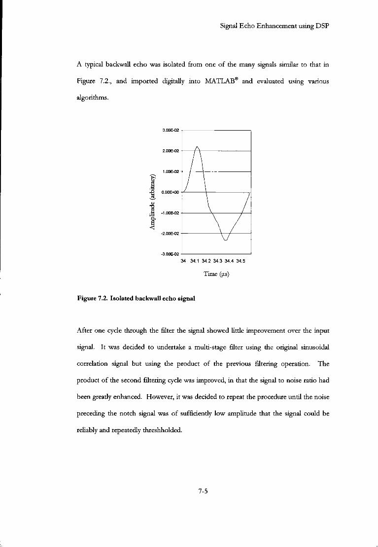
Signal Echo Enhancement using DSP
A typical backwall echo was isolated from one of the many signals similar to that in Figure 7.2., and imported digitally into MATLAB® and evaluated using various algorithms.
3.0OE-O2 -i 1
2.00E-02
1.00E-02
r O.OOE+00
1.00E-02
a 2.0OE-O2
-3.00E-02 J 1
34 34.1 34.2 34.3 34.4 34.5
Time ([AS)
Figure 7.2. Isolated backwall echo signal
After one cycle through the filter the signal showed kttle improvement over the input
signal. It was decided to undertake a multi-stage filter using the original sinusoidal
correlation signal but using the product of the previous filtering operation. The
product of the second filtering cycle was improved, in that the signal to noise ratio had
been gready enhanced. However, it was decided to repeat the procedure until the noise
preceding the notch signal was of sufficiendy low amplitude that the signal could be
reliably and repeatedly threshholded.
7-5
Signal Echo Enhancement using DSP
0.3
J -0.1
0.2
-0.3
10 20 30 40 Time ([JIS)
Figure 7.3. Signal after fourth filter cycle
As previously stated, because o f the way that FIR filters operate, they cause a delay in
the signal, and therefore every additional filtering operation causes additional delay.
This signal required an additional two cycles to give the result in Figure 7.3., totalling
four filter cycles. The signal to noise ratio was then re-calculated using the equation
4.19. for the filtered signal at 12.0dB.
The two signals were superimposed upon each other wi th the unfiltered signal shown
in blue and the filtered signal in red, as in Figure 7.4. showing a time delay, estimated at
2(xs, equating to a distance in the material o f 12mm. The signal time is taken f rom the
first point o f significant deviation, as shown in Figure 7.8. This time delay is only o f
relevance to the accuracy o f location o f a defect, but not in detection o f a defect.
7-6

Signal Echo Enhancement using DSP
o :4 •
0D3
O C I
•0.01 -
1 ^ 7
a Time delay -0C2
-0D3
... i 0 OS 1 15 2 2.5 3 3i 4 4.5 5
Time (|XS)10
Figure 7.4. Unfiltered signal (blue) and 4* cycle filtered signal (red), with markers
showing delay
7.4. Pass-band Filtering
The various filter parameter permutations available within the filter design and analysis
tool (EDATool) and signal processing toolbox were explored and applied to the signal.
The results were evaluated and o f the multitude o f parameter permutations, Figure 7.5.
shows the parameters o f the filter chosen wi th the best compromise o f signal time
delay and signal to noise ratio. Figure 7.6. shows the Tx3 Rx2 signal wi th the
application o f the 10 t h order FIR bandpass filter. Due to the linear-phase FIR filtering
process the resultant signal shows time delay as wi th the correlation filter. The delay
was measured by superimposing the filtered signal upon the unfiltered signal, as shown
in Figure 7.7. Figure 7.8. is a close up o f the two signals wi th the unfiltered signal i n
red and the bandpass signal in blue. The signal to noise ratio was then re-calculated,
using the equation 4.19. at 17.0dB for the band-pass filtered signal.
7-7
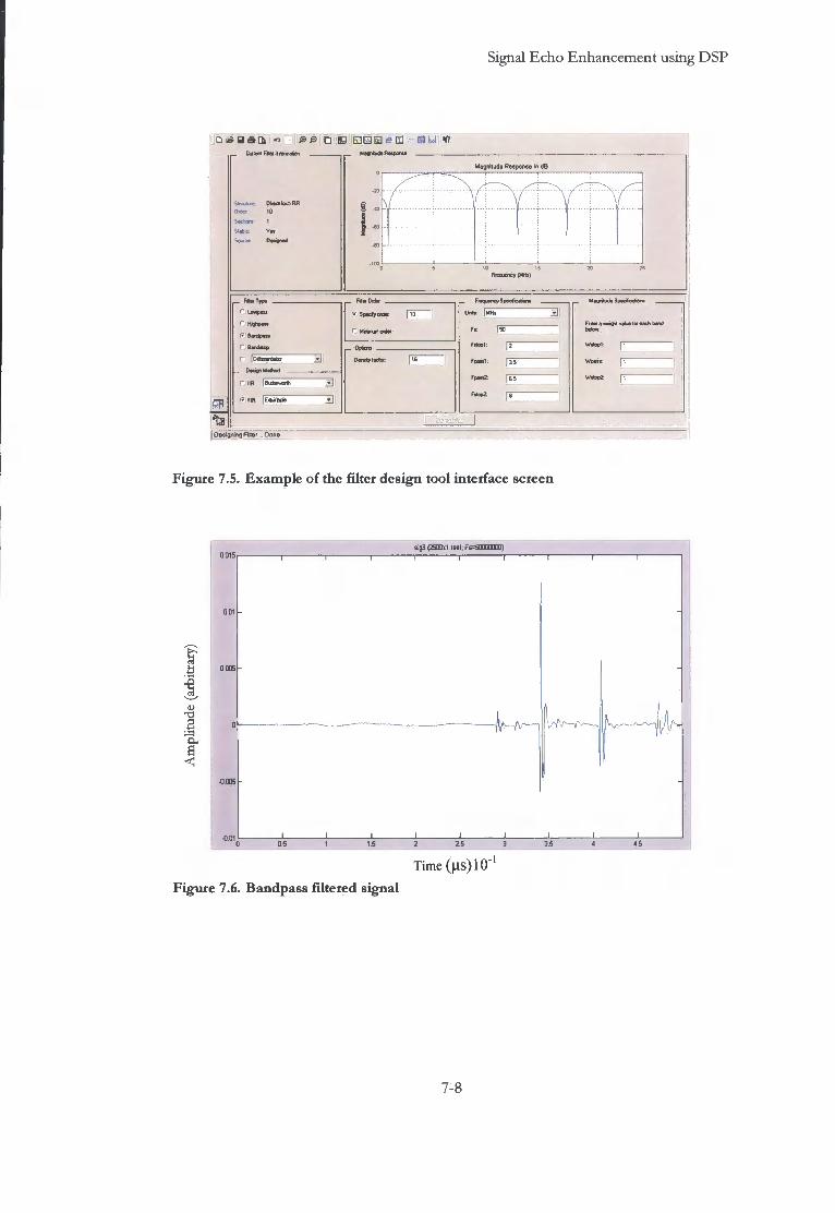
Signal Echo Enhancement using DSP
i y i . i l « Curiam Fytw
D 63 Q Q S i S a -Hsgntuda Rwponte
; . HI
Sktctmr DMC* for- FiP
S«ctem: 1
Sttbn V H
Magnitude Response in dB
Frequency SptsaScaaora
F* [SO
Ftttpl:
FpMt2:
Fftce2
(IT
Designing Fids' Done
Figure 7.5. Example of the filter design tool interface screen
Mas?*** Spadfieafeai.
Erta a value la eaai band
WPMC [i
5ig3 (2HBxl real, Fs=50QD00DD)
Time (jxs) 10"
Figure 7.6. Bandpass filtered signal
7-8
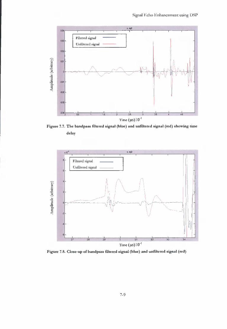
Signal Echo Enhancement using DSP
. . s i « 3
Filtered signal
Unfiltered signal
1 1
! 11 , 1.5
Time (}XS)10
Figure 7.7. The bandpass filtered signal (blue) and unfiltered signal (red) showing time
delay
a, sig3
Filtered signal
Unfiltered signal
I • T -
3 2 3 3 2 3 3 I 2 3
Time (us) 10
Figure 7.8. Close-up of bandpass filtered signal (blue) and unfiltered signal (red)
7-9
Signal Echo Enhancement using DSP
7.5. Filtering a Weak Echo Signal
It has being shown that Digital Signal Processing (DSP) can improve the signal to noise
ratio of the defect echo signal. However to this point the DSP had only been applied
to the signal from adjacent probes with the strongest echo signal, but to confirm the
choice of filter, it must also realise the defect from the weaker echo signals scattered
from the defect. The signals were re-examined and it was decided to use the signal
from the probe in position 3 with the probe in position 1 receiving the signal. This
signal had the least favourable SNR, calculated using the equation 4.19. as —5.5dB. The
notch echo was still distinguishable from the noise, however it would not be revealed
by signal thresholding methods.
7.6. Cross-correlation Filtering of a Weak Echo Signal
The first of the two most successful FIR filters form the previous experiment, the
cross-correlation filter, was applied to the weaker signal. The cross-correlation filter
used the same backwall echo signal (Figure 7.2.), as the previous experiment. This
enabled a true evaluation of the filter as it had been applied to both a strong and weak
echo signal. After the first cycle through the filter the signal showed litde improvement
over the input signal. It was decided to again employ a multi-stage filtering approach as
in the previous experiment. This was conducted using the original sinusoidal
correlation signal but using the product of the previous filtering operation. The
procedure was repeated through six cycles until the noise preceding the notch signal
was sufficiently low in amplitude that the signal could be reliably threshholded
7-10

Signal Echo Enhancement using DSP
!
I
Unfiltered signal
Filtered signal x 100
nut i
1 f f . r . i
0 1 / 4
•0025^ : : 5 5 :5 1 5 ' 5
Time (ns)10
Figure 7.9. Unfiltered signal (blue) and 6th cycle filtered signal (red) increased in
amplitude by 2 orders of magnitude
Figure 7.9. shows the unfiltered signal overlaid wi th the filtered signal, however the
filtered signal has been increased in amplitude by 2 orders o f magnitude to increase
visual clarity o f the graphical representation. The delay due to the filtering mechanism
was measured at 2.5us equating to a distance o f approximately 14.75mm in steel. The
signal to noise ratio was re-calculated at 9.5dB.
7.7. Pass-band Filtering of a Weak Echo Signal
The filter designed for theTx3 Rx2 signal, the 10 t h order FIR bandpass filter (Figure
7.8. ) , was applied to the weaker echo signal, Tx3 R x l . This enabled a true evaluation o f
the filter as i t had been applied to both a strong and weak echo signal.
7-11
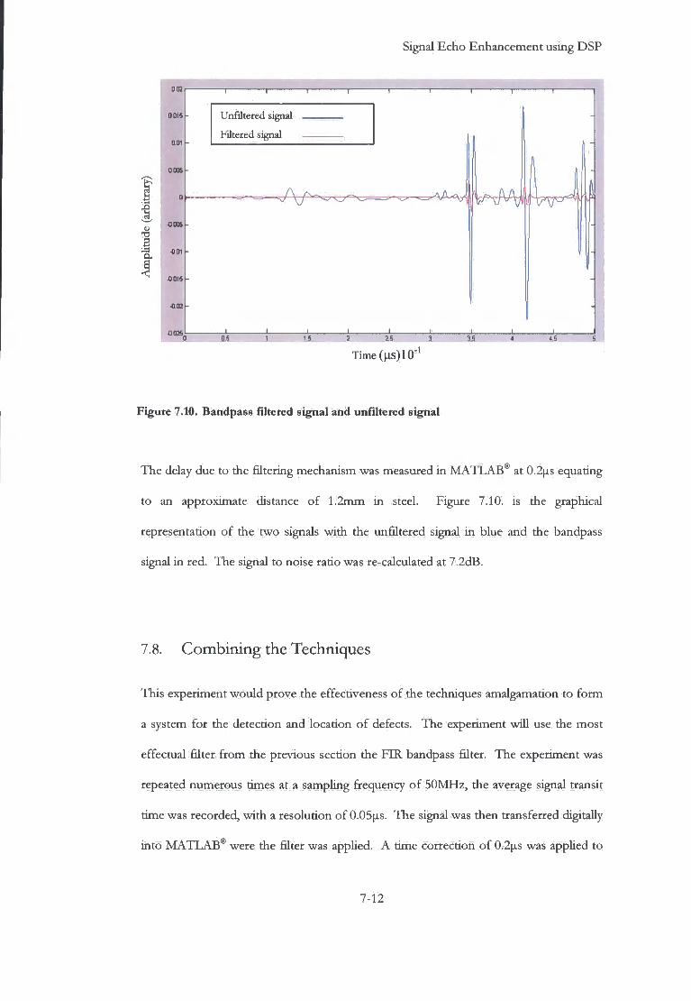
Signal Echo Enhancement using DSP
002
0005
r i -0.005 1
•5 -001
•0Q15
- i 1 1 r
Unfiltered signal
Filtered signal
05 15
Time(|XS)10
Figure 7.10. Bandpass filtered signal and unfiltered signal
The delay due to the filtering mechanism was measured in M A T L A B * at 0.2\xs equating
to an approximate distance o f 1.2mm in steel. Figure 7.10. is the graphical
representation o f the two signals with the unfiltered signal in blue and the bandpass
signal i n red. The signal to noise ratio was re-calculated at 7.2dB.
7.8. Combining the Techniques
This experiment would prove the effectiveness o f the techniques amalgamation to fo rm
a system for the detection and location o f defects. The experiment wi l l use the most
effectual filter f r o m the previous section the FIR bandpass filter. The experiment was
repeated numerous times at a sampling frequency o f 50MH2, the average signal transit
time was recorded, wi th a resolution o f 0.05us. The signal was then transferred digitally
into MATLAB® were the filter was applied. A time correction o f 0.2\xs was applied to
7-12

Signal Echo Enhancement using DSP
all the filtered signal times to compensate for the filtering effect. However the time of 0.2us is for the total transit time within the material, equating to 1.2mm, which is also the wavelength of the ultrasound within the material. This equates to a maximum effective location accuracy of X/2 (0.6mm) [8], even without the compensation, the location of the defect would not be overly affected. Table 7.1. displays the average of filtered times with the corresponding distances calculated using 5900 m/s for the speed of sound in steel and the relationship shown in Equation 7.1.
Table 7.1. Filtered signal path distance calculated at 5900m/sec
Distance (mm) Time (us)
Signal path +/-0.05 mm +/-0.05 us
A & B 184.10 31.20
A & C 180.50 30.60
B & C 172.90 29.30
The results displayed in Table 7.3. are the distances when 1.2mm is subtracted, to
compensate for the effect of the filter. The ellipse equations 6.1. and 6.2. were applied
to the corrected distances in Table 7.3. and the results plotted against the V I calibration
block.
Distance Velocity
= Transit Time [7.1.]
The difference in distances between the unfiltered signal and the filter-corrected signal
are listed in Table 7.4. This shows that the largest difference in distance is 0.60mm
(<0.5%), between probes 2 and 3, and is equivalent to the effective minimum defect
detection of half of the wave length (X/2) [8].
7-13

Signal Echo Enhancement using DSP
Table 7.3. Filtered signal path distance calculated at 5900m/sec
Signal path
Filtered signal distance (mm)
+/-0.05mm
Corrected distances (mm)
+/-0.05mm
A & B 184.10 182.90
A & C 180.50 179.30
B & C 172.90 171.70
Table 7.4. Signal path distance differences
Signal path
Unfiltered distance
+/-0.05mm
Filtered and corrected
distances
+/-0.05 mm
Difference between
filtered and
unfiltered distance
A & B 182.60mm 182.90mm 0.30mm
A & C 179.40mm 179.30mm 0.10mm
B & C 172.30mm 171.70mm 0.60mm
Table 7.5. Signal to Noise Ratios (dB)
Probe Pairs Unfiltered Signal Bandpass filtered
Signal
Correlation Filtered
Signal
Tx3 Rx2 signal -2.0dB 12.0dB 17.0dB
Tx3 Rxl signal -5.5dB 7.2dB 9.5dB
Two variations of FIR filters were evaluated, a bandpass filter and a correlation filter
using an isolated backwall echo as the filter signal. The signal required several passes
through the correlation filter to effectively improve the signal to noise ratio (Table 7.5.)
7-14
Signal Echo Enhancement using DSP
7.9. Conclusion
The first section of this chapter investigated the half ellipses as a geometric method of
locating a defect. The experimental work conducted in this chapter show that the
technique could be adapted the to locate the defect on the bottom surface of the V I
calibration block. The use of three probes and the combination of signal paths
provided data to locate the notch, using the intersection of the three ellipses, to an
accuracy of <0.5% of the transit distance. However, the weaker echo signals required a
subjective approach in their time estimation.
The MATLAB® filter design and analysis tool (FDATool) and signal processing
toolbox (SPTool) were employed to design and develop a FIR bandpass filter, and
effectively apply the filter to the signals. The developed filter was similar in its
effectiveness to the correlation filter in improving the signal to noise ratio. However,
the time delay imparted upon the signal was a tenth of that of the correlation filter, and
thereby chosen as the most effectual filter for this application, with the SNR results
shown in Table 7.5. The application of the FIR bandpass filter to the weaker echo
signals enabled the signal to be thresholded, and thereby objectively measure their
transit times. The application of the ellipse geometry equations to the FIR filtered
signals proved that the techniques were compatible and that with relatively basic signal
time correction the defect could be located.
This work was presented at the 30 t h Annual Review of Progress in Quantitative Non
destructive Evaluation (QNDE) July 27-August 1, 2003, held in Green Bay, Wisconsin
U.SA. Also a modified version of this work was published in the journal, Non
destructive Testing and Evaluation [9]
7-15
Signal Echo Enhancement using DSP
7 .10 . References
1. Kuo, M.K., T.R. Lin, P.L. Liu, and T.T. Wu, Locating the crack tip of a surface-breaking crack. Parti. Line crack. Ultrasonics, 1998. 36: p. 803-811.
2. Kazanavicius, E., A. Mikuckas, I . Mikuckiene, and V. Kazanavicius, Noisy signal processing in real time DSP systems. Ultragarsas Journal, 2003. 46(1): p. 31-36.
3. Birks, A.S. and R.E. Green Jr., Ultrasonic Testing. 2nd ed. Nondestructive Testing Handbook, ed. P. Mclntire. Vol. 7. 1991, Baltimore, Maryland, U.S.A.: American Society for Nondestructive Testing. 893.
4. Fomitchev, M.I . , Y.E. Grigorashvily, and S. Volkov, Ultrasonic pulse shaping with optimal lag. International Journal of Imaging Systems and Technology, 1999. 10(5): p. 397-403.
5. Chen, J., Y. Shi, and S. Shi, Noise analysis of digital ultrasonic nondestructive evaluation system. International Journal of Pressure Vessels and Piping, 1999. 76(9): p. 619-630.
6. Smith I I I , J.O., Mathematics of the Discrete "Fourier Transform (DFT), with Music and Audio Applications. 2003, Stanford, California: W3K Publishing.
7. Hasnselman, D. and B. Littlefield, Mastering MATLAB 6: A Comprehensive Tutorial and Reference. 2001, New Jersey: Prentice Hall.
8. Diederichs, R., The Online Journal of Nondestructive Testing. 2005, www.ndt.net.
9. Snowdon, P.C., S. Johnstone, and S. Dewey, A 2D Static Ultrasonic Array of Passive Probesfor Improved Probability of Detection. Nondestructive Testing And Evaluation, 2003.19(3): p. 111-120.
7-16
Multi-Probe Scan
Chapter 8.
Multi-Probe Scan
8.1. Introduction
The project remit required that the inspection be carried out on an immersed and
moving steel billet. This required two additional variables into the development of the
system. I t was decided that the immersion section of the project be conducted as the
last section of the project. The moving billet experiment would be conducted by
indexing the transducer array by a specific distance after each individual pulse
examination was conducted. This procedure will then be repeated over the designated
area of the V I block to be examined.
As previously stated in section 2.2. of this thesis, each individual 10mm diameter probe
is firing every 8mm of billet, when travelling at lm/s. However the scans for this
experiment will be conducted in 1mm increments, this being the lower figure of the 1-
2mm that is stated by Wolfram (2000) [1], equating to 60 individual A-scans of the V I
block.
8-1

Multi-Probe Scan
This chapter wi l l also bring together the elements o f the project that f o r m the Normal Probe Dif f rac t ion technique (NPD) the term given to the amalgamation o f the processes elements. These elements comprise o f the scanning o f the billet, ellipse geometry location o f the defect, and the Digital Signal Processing.
8.2. Detection Limits
This experiment would be completed using the V I calibration block utilised as the test
material. I t was necessary to ascertain the extent o f the region o f which the passive
probes could receive the diffracted signal f r o m the notch. This would minimise the
quantity o f individual readings required o f each scan. The method was to use two
probes, one as the dedicated transmitter the other as the receiver, and scan the V I
block maintaining the 22.5mm probe separation.
Probe separation 22.5mm
3 Direction of scan
Figure 8.1. Probe positions and direction scan
8-2

Multi-Probe Scan
The transducer array scanned the V I block unti l the notch signal was indistinguishable
f r o m that o f the background noise. The starting position o f the probes was wi th the
transmitting probe positioned directly over the notch, and the receiver over the 100mm
bottom surface (Figure 8.1.). The experiment was repeated numerous times, alternating
the probes used and their position within the two probe array.
The results were collated and filtered wi th the FIR filter designed in the previous
chapter (section 7.6.), using Microsoft E X C E L and MATLAB®. The signal threshold
for this experiment was set at 6dB Signal to Noise Ratio and any signal above this
would indicate positive defect detection.
Probability of Detection
P/E 100 -• - - - NPD r 80 -•
60
40 ••
20 -•
0
/ 1 45 42 39 36 33 30 27 24 21 18 15 12 9 6 3 0
Distance from Defect (mm)
Figure 8.2. Comparison of Probability of Detection for NPD and Pulse-Echo
8-3

Multi-Probe Scan
The scans showed that the diffracted signal was detectable by the passive probe, when
the receiver was over 42mm from the notch and the transmitter 20mm from the notch.
Figure 8.2. shows the increase of detection ability using the standard single-probe-
multi-receiver scan over the conventional single-probe pulse/echo scan. It shows that
the NPD system starts detecting the defect at a lateral distance of 41mm from the
defect whereas the pulse-echo probe needs to be within a range of 15mm. However, at
the 41mm distance the reliability of detection was erratic, and only became stable when
the distance from the notch was less than 35mm (Figure 8.2.) The detection limit is
defined by Birks (1991) as the smallest measurement having a probability of 97.5% of
not being caused by noise [2]. The application of the limits advocated by Birks, equates
to a distance from the notch of 33mm. From these results it was decided to scan for
60mm, i.e. 30mm either side of the notch.
8.3. Scanning the V I Block
The method was to use two probes, one as the dedicated transmitter the other as the
receiver, and scan the V I block mamtaining the 22.5mm probe separation. The starting
position of the probes array was with the centre of the array 30mm from the notch,
with the transmitting probe facing the radius of the V I block (Figure 8.3.). The scan
was conducted in 1mm increments, being the lower figure of the l-2mm that is stated
by Wolfram (2000) [1], that is 60 individual A-scans of the V I block.
8-4

Multi-Probe Scan
T o make the data more manageable and easier to analyse, a matrix was formed f r o m the data using Microsoft E X C E L , allowing the A-scans to be stacked, creating a B-scan o f the V I block (Chapter 3.2.) [3].
Probe separation 22.5mm
I i
Centreline of Direction of scan probe array
Figure 8.3. Probe transmitter/receiver location and direction of scan
The collated data was interrogated wi th the B-scan result plotted in Figure 8.4. wi th the
first 20\xs o f the signals removed as it contained no relevant data. Removing the first
20\xs o f the signals and concentrating on the defect also negated the lengthy process o f
filtering the 60 individual A-scans. The filtering o f the scan would be added to the
process later in the experiment.
The greyscale B-scan shows all o f the features o f the V I block, the 100mm backwall,
the notch and the 91mm backwall, that are recognised by their time position on the
scan. However, the greyscale graduation can be adjusted for the signal amplitude,
effectively making it a signal threshold, and required some diligence in ensuring a linear
scale.
8-5
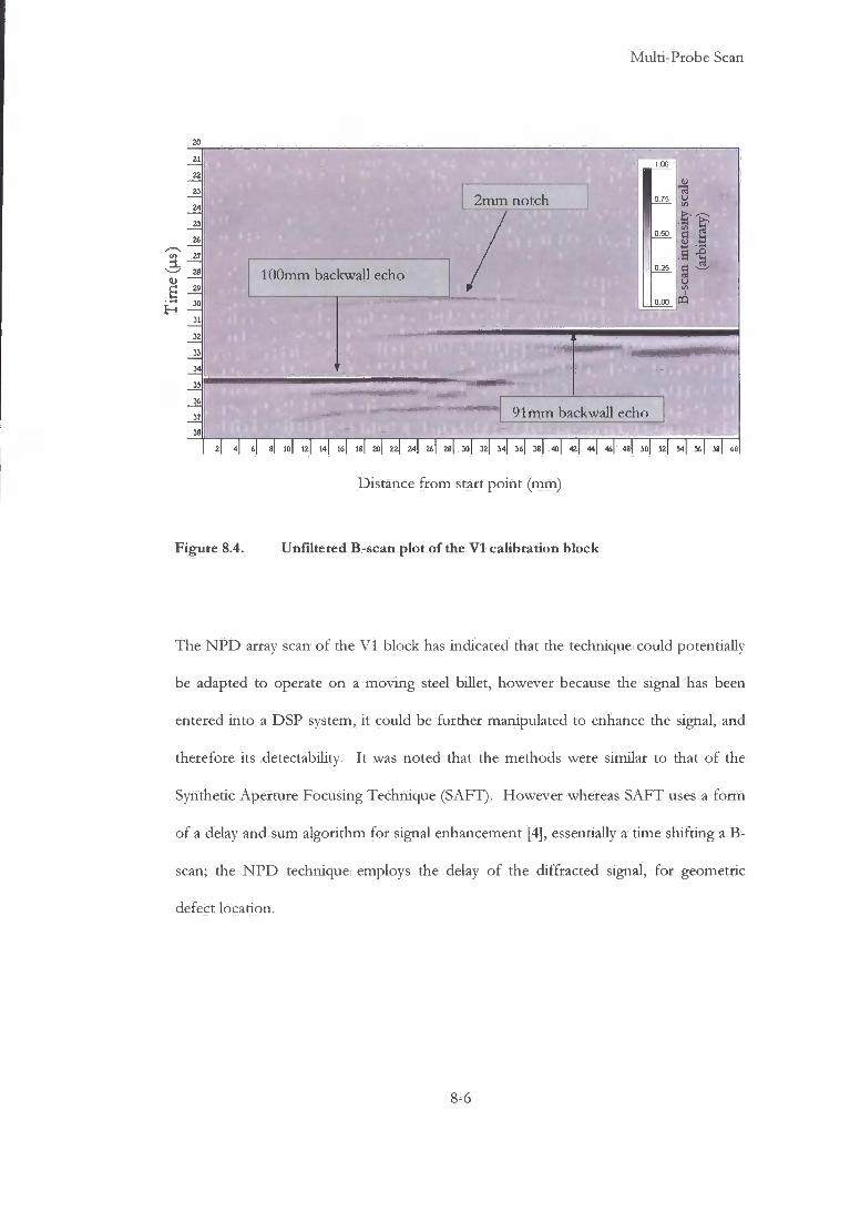
Multi-Probe Scan
2mm notch
100mm backwall echo
91mm backwall echo
10 12 14 16 18 20 22 24 26 23 JO 32 3 4 3 6 38 40 42 44 46 48 50 52 54 56 58 60
Distance f r o m start point (mm)
Figure 8.4. Unfiltered B-scan plot of the V I calibration block
The N P D array scan o f the V I block has indicated that the technique could potentially
be adapted to operate on a moving steel billet, however because the signal has been
entered into a DSP system, it could be further manipulated to enhance the signal, and
therefore its detectability. I t was noted that the methods were similar to that o f the
Synthetic Aperture Focusing Technique (SAFT). However whereas SAFT uses a f o r m
o f a delay and sum algorithm for signal enhancement [4], essentially a time shifting a B-
scan; the N P D technique employs the delay o f the diffracted signal, for geometric
defect location.
8-6

Multi-Probe Scan
8.4. Filtering the B-scan
2mm notch
100mm backwall echo
1.00
M 0 75
I 0.50
1
f t .s -e
(4
91mm backwall
2| 4| 6 S| 101 121 141 16| 181 20 1 22 | 24| 26| 2S| 301 32| 34| 361 3S| 401 42| 441 461 481 50| 521 5«\ 56\ 581 60
Distance from start point (mm)
Figure 8.5. Filtered B-scan plot of the V I calibration block
The digital data that formed the B-Scan o f the previous experiment was imported into
MATLAB® to be filtered. The previously developed filter, die FIR filter designed in
chapter (Chapter 7.6.), was applied to the signals. The resultant signals were collated,
stacked and plotted out graphically re-forming the B-scan. The application o f this filter
would facilitate the application o f a defect detection threshold level enabling the defect
to be detected automated system. The filtered B-scan in Figure 8.5. shows much less
noise and the features are clearly defined, wi th the notch at 29(is, the 100mm backwall
at 34\xs and the 91mm backwall at 31 us.
8-7
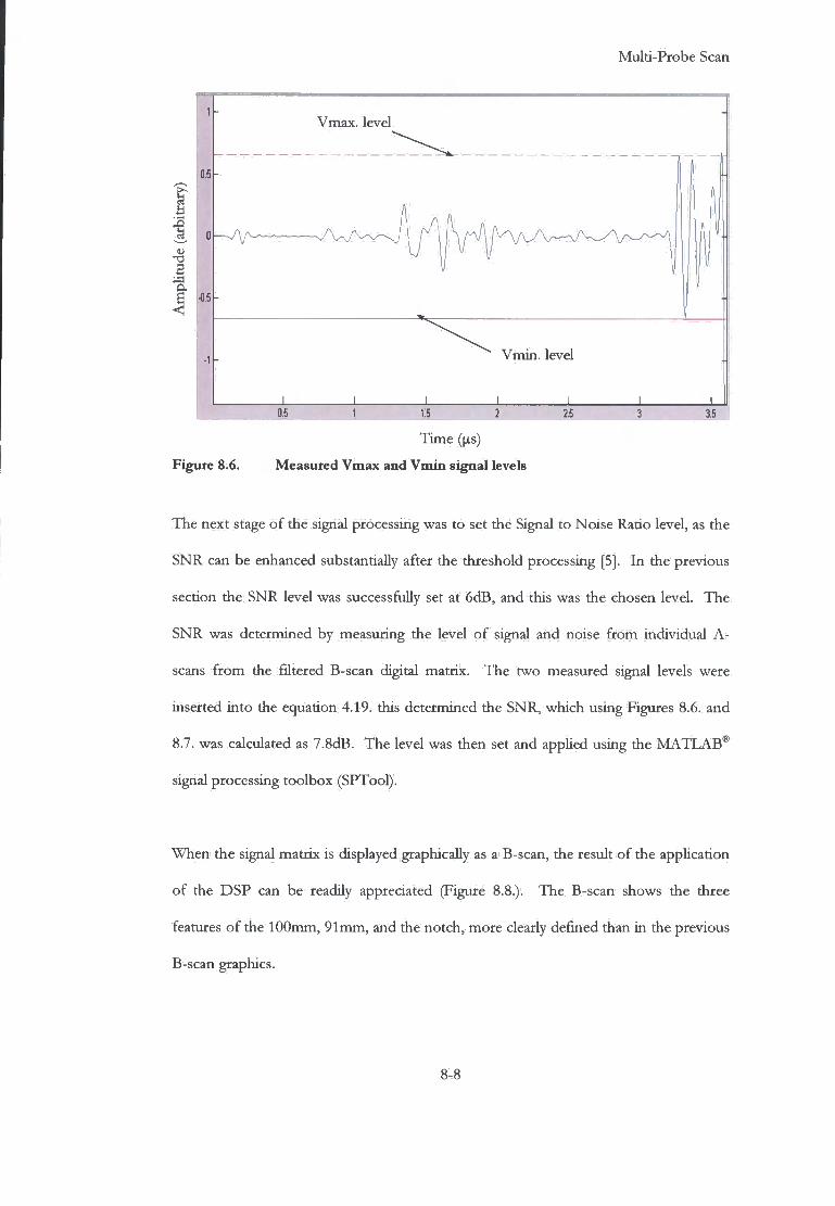
Multi-Probe Scan
Vmax. level
1
0
a -0-5 r 9.
Vmin . level
5 1.5 3.5 2 25 3
Time (^s)
Figure 8.6. Measured Vmax and Vmin signal levels
The next stage o f the signal processing was to set the Signal to Noise Ratio level, as the
SNR can be enhanced substantially after the threshold processing [5]. I n the previous
section the SNR level was successfully set at 6dB, and this was the chosen level. The
SNR was determined by measuring the level o f signal and noise f r o m individual A -
scans f r o m the filtered B-scan digital matrix. The two measured signal levels were
inserted into the equation 4.19. this determined the SNR, which using Figures 8.6. and
8.7. was calculated as 7.8dB. The level was then set and applied using the MATLAB®
signal processing toolbox (SPTool).
When the signal matrix is displayed graphically as a B-scan, the result o f the application
o f the DSP can be readily appreciated (Figure 8.8.). The B-scan shows the three
features o f the 100mm, 91mm, and the notch, more clearly defined than in the previous
B-scan graphics.

Multi-Probe Scan
i
Vmax. level
-0 5
Vrnin. level
OS 1 5 1
Time (us)
Figure 8.7. Measured Vmax and Vmin noise level
j
21 1 00
M 0.75
JLSL
22 'J
2mm Notch 23 : 7l V3
24
r 91mm Backwall ojo. a 100mm Backwall 26
•7 ox c •
29 0.00 ffl
30
31
32
:l 1
35
-r,
37
'••»
0 j | 4| 6\ i\ 101 121 u | 1 es| t s ] 20[ 22[ 2<f| 261 28 301 32 34| 361 3S| 401 421 44j 461 481 501 521 54| 561 581 60
Distance from start point (mm)
Figure 8.8. Filtered and thresholded B-scan plot of the V I calibration block
8-9

Multi-Probe Scan
8.5. The NPD System
Described in this section is the layout design o f the potential automated defect
detection system, incorporating all o f the successful elements developed during the
project. The order i n which the individual elements are positioned within the system is
significant. The positioning within is required to maximise the processing power and to
minimise the overall financial cost. A block diagram was designed and drawn for the
proposed system, and is displayed in Figure 8.9.
Pulser Flaw detector Flaw detector
Receiver
Signal out
Echo signal
Alarm
Digital Signal Processing
FIR Filter
Time correction
Threshold level
Ellipse calculations
Read-out of defect locations
A
1 No further action
Figure 8.9. Block diagram of the proposed system
8-10
Multi-Probe Scan
The ultrasonic pulse is generated in a generic transmitter/receiver — flaw detection
system, with the received signal being diverted into the Digital Signal Processor. The
signal is then filtered to maximise defect detection, and time corrected, to remove the
delay imparted during the F I R filtering process. It is envisaged that the filtering process
could have variable parameters, depending upon the input frequency. The threshold
level may require a parameter variance, dependent upon material dimensions and
sensitivity required. The output signal now has two alternatives. This is dependent
upon how the threshold D S P has categorised the signal as either defect, or no-defect.
I f no-defect is registered, then no further action is required. I f however a defect has
been identified, then the signal remains within the DSP system for additional
processing. This additional processing is the application of the ellipse equations for the
geometric location and positioning of the defect. The data on the defect could be
displayed as 3-dimensional co-ordinates, or be graphically displayed.
8-11
Multi-Probe Scan
8.6. Conclusion
The project required that the inspection be carried out on an immersed and moving
steel billet. The immersion experiments are conducted later in the project, in Chapter
10. Indexing the probes a specific distance over the billet and recording the individual
A-scans overcame the problem of conducting the examination on a moving billet,
successfully simulating the billet traversing the probe array.
The extent of the region of which the passive probes could receive the diffracted signal
from the notch was ascertained to minimise the length of the scan. These scans
showed that the diffracted signal was detectable at over 40mm from the notch by the
passive probe receiver, after filtering. The results indicated that the signal could be
reliably and repeatedly detected from a distance from the probes of 33mm from the
defect with a >6dB Signal to Noise Ratio.
The results from the unfiltered scan (Figure 8.4.) showed that the passive probe could
reliably define the features within the V I block. The unfiltered B-scan showed a
graininess indicating background noise; also, the graphics displayed long diffraction arcs
from the notch. Once the filtering process had been applied (Figure 8.5.), the B-scan
was cleaner in appearance with the notch in particular being more clearly defined.
The next stage of the filtering process was to threshold the filtered signal, this proved
to be successful as the background noise and the diffraction arc from the notch were
8-12

Multi-Probe Scan
effectively filtered out (Figure 8.8.). The process demonstrates that time of flight diffraction can be realized using passive normal probes (Normal Probe Diffraction, N P D ) to effectively locate and realise defects.
The use of a N P D system could increase the throughput speed of the steel billet due to
its increase of volumetric inspection per individual transducer pulse. A proposed
system was designed and laid out in the form of a block diagram and is displayed in
Figure 8.9., with the various elements shown in there relative positions. The design of a
working system will be addressed in the final chapter, conclusions and further work.
The first section of this chapter covering the signal detection limits and the filtering of
the signal matrix formed part of a poster presented at The 31 s t Annual Review of
Progress in Quantitative Non-destructive Evaluation ( Q N D E ) held in Golden,
Colorado U.S.A. 2004.
A journal paper based upon this work was presented at The 42nd Annual British
Conference on N D T held in Bransford, Worcester U .K. on 16-18 September 2003, and
subsequently published in the Insight journal of the British Institute of Non-
Destructive Testing [6].
8-13
Multi-Probe Scan
References
Wolfram, A. Automated ultrasonic inspection, in 15th WCNDT conference. 2000. Rome, Italy: www.karldeutsch.de/PDF/Automated U T inspection MayOO.PDF.
Birks, A.S. and R . E . Green Jr., Ultrasonic Testing. 2nd ed. Nondestructive Testing Handbook, ed. P. Mclntire. Vol. 7. 1991, Baltimore, Maryland, U.S.A.: American Society for Nondestructive Testing. 893.
Hellier, C.J. , Handbook of Nondestructive Evaluation. 2001, New York, U.S.A.: McGraw-Hill.
Lingvall, F . , A method of improving overall resolution in ultrasonic array imaging using spatio-temporal deconvolution. Ultrasonics, 2004. 42: p. 961-968.
Chen, J . , et al., Noise analysis of digital ultrasonic nondestructive evaluation system. International Journal of Pressure Vessels and Piping, 1999. 76(9): p. 619-630.
Snowdon, P.C. , et al.,^4 2D Static Ultrasonic Array of Passive Probesfor Improved Probability of Detection. Nondestructive Testing And Evaluation, 2003.19(3): p. 111-120.
8-14

N P D Applied to a Section of Steel Billet
Chapter 9.
NPD Applied to a Section of Steel Billet
9.1. Introduction
The application of the developed technique has so far been conducted using a known
test sample containing a pseudo defect, the V I calibration block. In this chapter, the
technique is applied to the original 70mm x 70mm section of steel billet first used in
Chapter 5 of this thesis. The first part of this chapter describes the general experiment
set-up using an immersion multi-probe transmitter/receiver array and a 2.5mm
diameter 10mm deep flat-bottomed hole as a simulated defect machined into the steel
billet. The identical inspection is then repeated on a billet containing a defect produced
during its manufacture.
This series of experiments completes the remit of the project and the investigation into
the development of a potential system or techniques' using an array of normal angle
immersion probes for billet inspection. Geometric defect location using ellipse
calculations have been characterised in numerous previous experiments, and will
therefore not form part of the final series of tests.
9-1

N P D Applied to a Section o f Steel Billet
9.2. General Experimental Set-Up
A section o f steel billet was characterised in terms o f the presence and approximate
location o f defects using a single probe pulse-echo method. A defect was then
simulated in the section by machining a 2.5mm diameter flat-bottomed hole machined
to a depth o f 10mm [1]. The use o f a flat-bottomed hole is a standard method for
characterising defect detection instrumentation. The following series o f experiments
are conducted as immersion tests, and use a similar stand o f f distance o f 70mm, to that
o f the bar mil l . The probes were held stationary above the billet, while the billet was
indexed passed the array. The temperature o f the water was thermostatically regulated
at 24 + / - 1 degrees Celsius, as this is above that o f the ambient temperature o f room,
and was chosen to give consistent readings regardless o f the surrounding environmental
conditions. The set-up was pre-tested to ensure that the indexing mechanism operated
as expected, wi th the probe holder remained static over the period o f the tests (Figure
9.1.)
Probe holder
Steel billet /
Probes
Figure 9.1. Photograph of an immersion set-up used during initial pre-trials
9-2

N P D Applied to a Section o f Steel Billet
The Doppler effect o f the propagating wave through the moving billet was also considered. Using equation 7.1. and with the wave front propagating at 5900m/s, the signal transit time through the 70mm square section steel billet is 23.73us. The transit time o f the signal within the water was also calculated using a signal velocity o f 1480m/s as 94.59 \is. Therefore wi th the steel billet moving at l m / s , the billet wi l l have moved 0.11832 mm, during the 118.32us, and was considered negligible. Numerous individual A-scans were conducted over the section o f the billet containing the 10mm deep, 2.5mm diameter flat-bottomed hole defect, to ensure that the investigation was conducted over the correct section o f steel billet.
9.3. Immersion Inspection of a 2. 5mm Flat-bottomed Hole
Probe separation 22.5mm
I I r n
Centre of two-probe array * Direction of scan
Centre of two-probe array *
•
30mm 30mm 4 'w 1 i i 1
2 5mm flat-bottomed hole 10mm deep
Figure 9.2. Drawing of the immersion set-up used for the flat-bottomed hole test
9-3
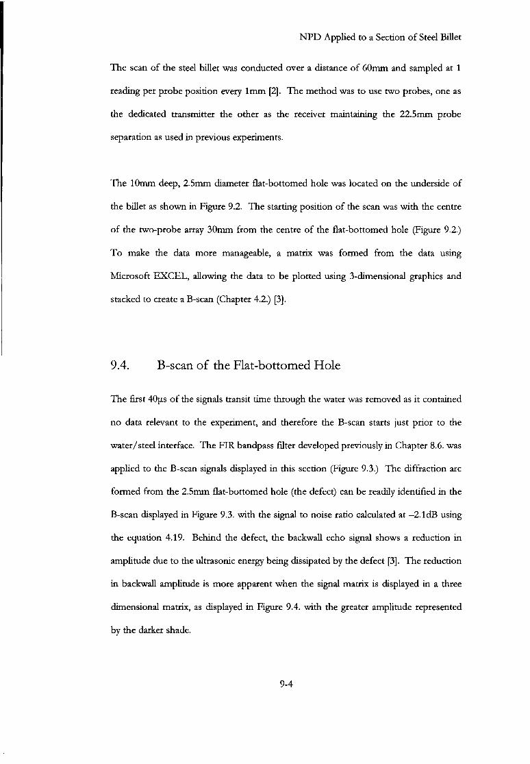
N P D Applied to a Section of Steel Billet
The scan of the steel billet was conducted over a distance of 60mm and sampled at 1 reading per probe position every 1mm [2]. The method was to use two probes, one as the dedicated transmitter the other as the receiver maintaining the 22.5mm probe separation as used in previous experiments.
The 10mm deep, 2.5mm diameter flat-bottomed hole was located on the underside of
the billet as shown in Figure 9.2. The starting position of the scan was with the centre
of the two-probe array 30mm from the centre of the flat-bottomed hole (Figure 9.2.)
To make the data more manageable, a matrix was formed from the data using
Microsoft E X C E L , allowing the data to be plotted using 3-dimensional graphics and
stacked to create a B-scan (Chapter 4.2.) [3].
9.4. B-scan of the Flat-bottomed Hole
The first 40us of the signals transit time through the water was removed as it contained
no data relevant to the experiment, and therefore the B-scan starts just prior to the
water/steel interface. The F I R bandpass filter developed previously in Chapter 8.6. was
applied to the B-scan signals displayed in this section (Figure 9.3.) The diffraction arc
formed from the 2.5mm flat-bottomed hole (the defect) can be readily identified in the
B-scan displayed in Figure 9.3. with the signal to noise ratio calculated at -2.1dB using
the equation 4.19. Behind the defect, the backwall echo signal shows a reduction in
amplitude due to the ultrasonic energy being dissipated by the defect [3]. The reduction
in backwall amplitude is more apparent when the signal matrix is displayed in a three
dimensional matrix, as displayed in Figure 9.4. with the greater amplitude represented
by the darker shade.
9-4

N P D Applied to a Section o f Steel Billet
60 1.00
'r. •f.
.3 c
i
40 41 42 40 41 42 43 44 45 48 47 48 49 50 51 52 53
Time (us)
Figure 9.3. B-scan of 2.5mm flat-bottomed hole
Time (us)
42 44 46 48 5Q 52 Linear !
Distance Bickwall echo (mm)
-0.015
•0.005 X I
0.005
0 01
Figure 9.4. 3D time domain data display of 2.5mm flat-bottomed hole
9-5

N P D Applied to a Section o f Steel Billet
9.5. NPD applied to a Naturally Occurring Discontinuity
The next experiment carried out on the steel billet required the use o f all o f the
positions o f the probe array holder (Figure 3.3.) The central probe position o f the array
used as the dedicated transmitter (Figure 9.5.) The diagram in Figure 9.5. shows the
probe array holder over the steel billet, wi th the positions o f the probes labelled A to H ,
wi th the probe in position E as the dedicated transmitter. As previously stated in
section 4.2. the oscilloscope has only two input channels and therefore the experiment
required the receiving probes position, wi thin the probe holder, to be alternated to
simulate a complete array. The scan was conducted over a distance o f 60mm and
sampled at 1 reading per probe position every 1mm [2].
Flat-bottomed hole
Steel Billet
Probe Array
Probe Holder © C D © • © <§> ©
© ©
Figure 9.5. Diagram of the probe holder showing billet with flat-bottomed hole
and probe array
The signal corresponding to a reflection f r o m the signal can be seen on several o f the
unfiltered B-scans and indicate that the defect is identifiable by visual observation wi th
the passive probes. However, because o f the way B-scans display the signal i.e. they are
A-scans rotated 90 degrees around they-axis and stacked, the defect is not as readily
recognisable as in previous experiments displayed in A-scans.
9-6

NPD Applied to a Section of Steel Billet
0.1 •Defect
0.1 Backwall
0.2
— i 1 1 1 1 1
54 55 56 « 58 59 60 Time ((is)
Figure 9.6. A-scan from a typical section of steel billet (Probe D at 17mm)
50 1.00
50
D.75 3 40
•a 0 30 0 5L
20 3 5 0.26
a 1 ° •
03
54 55 56 57 58 59 60
Time ((is)
Figure 9.7. B-scan showing defect arc taken from Probe D
9-7
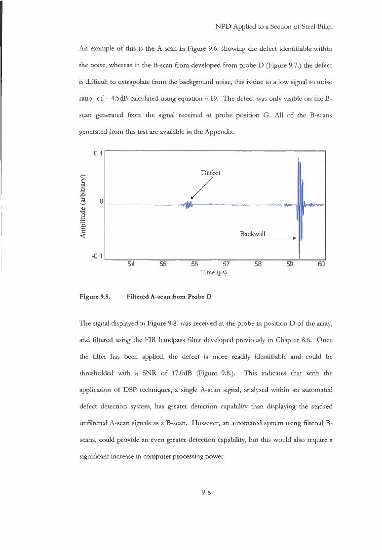
NPD Applied to a Section of Steel Billet
An example of this is the A-scan in Figure 9.6. showing the defect identifiable within the noise, whereas in the B-scan from developed from probe D (Figure 9.7.) the defect is difficult to extrapolate from the background noise, this is due to a low signal to noise ratio of - 4.5dB calculated using equation 4.19. The defect was only visible on the B-scan generated from the signal received at probe position G. All of the B-scans generated from this test are available in the Appendix.
0.1
L Defect
0
Backwall
-0.1 | 54 55 56 57 58 59 60
Time (|is)
Figure 9.8. Filtered A-scan from Probe D
The signal displayed in Figure 9.8. was received at the probe in position D of the array,
and filtered using the FIR bandpass filter developed previously in Chapter 8.6. Once
the filter has been applied, the defect is more readily identifiable and could be
thresholded with a SNR of 17.0dB (Figure 9.8.). This indicates that with the
application of DSP techniques, a single A-scan signal, analysed within an automated
defect detection system, has greater detection capability than displaying the stacked
unfiltered A-scan signals as a B-scan. However, an automated system using filtered B-
scans, could provide an even greater detection capability, but this would also require a
significant increase in computer processing power.
9-8
NPD Applied to a Section of Steel Billet
9.6. Conclusion
The geometric defect location using the ellipse calculations have been proved in
numerous previous static billet experiments. However it would require a significant
amount of development time to be successfully adapted for use on a moving steel billet.
As the project contained time constraints, it was decided that the geometric location
method would not be included in the final series of tests.
The application of the NPD technique had up to this chapter been developed only
using the V I calibration block as a test sample. During these experiments, the
technique detected the 2mm notch that was used as a defect with a SNR of -1.5dB.
However, because of the additional complexities associated with immersion testing
coupled with the extra problems of mode conversions, refraction etc., the technique
would therefore require additional development to be employed on a moving
submersed steel billet.
In this final chapter of the thesis, the technique was applied to a section of steel billet
70mm x 70mm in cross-section. A 2.5mm flat-bottomed hole was used as defect, and a
pseudo scan was conducted on the billet (Figure 9.3.). The 2.5mm flat-bottomed hole
was apparent in the B-scan, through the diffraction arc formed, and thereby detecting
the flat-bottomed hole with a SNR of -2.1dB using the NPD process.
The technique was subsequently applied to the section of steel billet with a naturally
formed discontinuity. The defect was located prior to the NPD scan using a single
pulse/echo probe scan, and conducted to ensure that a discontinuity was present in the
section under inspection.
9-9
NPD Applied to a Section of Steel Billet
The scan was conducted using all of the positions of the array, with each individual probe giving a different perspective of the defect. Several of the probes did not indicate the presence of the defect. This is due to the shape of the defect or unfavourable defect orientation in relation to the probes concerned. The SNR was improved significandy from -4.5dB of the unfiltered signal to 17.0dB using the technique.
The remaining probes received an echo signal from the defect of varying clarity.
Because the defect was naturally formed void with an uneven surface structure, how the
signals arrived at the transducers (diffraction, reflection, refraction etc.) was uncertain,
however the signal was successfully interpreted and the defect detected.
The displaying of the signals as filtered A-scan stacked to form B-scans is the simplest
way of displaying the signals resulting from the application of the NPD technique. Due
to the amount of data involved, it is the only practical method for manual inspection, as
i f the data was displayed as A-scans, 420 individual A-scans would have required
analysis. This requires the designed automated system to have sufficient digital signal
processing power to manipulate the volume of data received.
The experimental work conducted during this project has repeatedly proved that under
laboratory conditions, the use of the passive probes in conjunction with the application
of DSP can enhance the detection of discontinuities within steel sections.
9-10

NPD Applied to a Section of Steel Billet
References
Birks, A.S. and R.E. Green Jr., Ultrasonic Testing. 2nd ed. Nondestructive Testing Handbook, ed. P. Mclntire. Vol. 7. 1991, Baltimore, Maryland, U.S.A.: American Society for Nondestructive Testing. 893.
Wolfram, A. Automated ultrasonic inspection, in WCNDT conference. 2000. Rome, Italy. www.karldeutsch.de/PDF/Automated_UT_inspection_May 00
Hellier, C.J., Handbook of Nondestructive Evaluation. 2001, New York, U.S.A.: McGraw-Hill.
9-11
Conclusions and Further Work
Chapter 10.
Conclusions and Further work
The remit of the project was to investigate and develop the present ultrasonic system
currently employed at the steel mill. The motivation being that the system is not being
fully utilised to its full potential in that only one probe, within the array, is in use at any
time. Therefore, i f more than one probe or all probes could be simultaneously used,
the system could be operated more effectively, theoretically leading to a faster
throughput of inspected material, or increased defect detection sensitivity, or higher
reliability of defect detection, or a combination of the gains. The system developed in
this project was initially to be designed as an immersion technique using an array of
normal angle probes used for billet inspection. However the technique developed is
potentially transferable to other ultrasonic multi-probe array applications.
The preliminary experiment of the project was conducted on a section of steel billet,
and proved inconclusive due to the received signals being complex and not immediately
interpretable. This was due partly to the fact that the defect was large and unknown
and it was decided that there were too many variables for the initial experiment.
10-1

Conclusions and Further Work
Because of the complexities of signal trace, it was decided to eliminate as many of these variables as possible. The subsequent series of experiments were therefore carried out on a subject containing a simple known target.
It was decided to use a V I calibration block as the quality of the material could be
assured [1], and the 2mm notch could be utilized as a pseudo defect. The first series of
experiments on the V I block indicated that the signal from the 2mm notch was
detectable from outside that of specular reflection. Also, at 13 degrees away from the
centreline of maximum intensity; the notch was also outside of the stated 20dB drop
inspection zone of the main ultrasonic lobe [2]. This required a form of non-specular
reflection as the method of signal propagation. The probable method of this being
diffraction, because diffuse reflection requires a rough surface and the boundary
variations to be of the same order of magnitude or larger than the ultrasound
wavelength being used [3], and the V I block had a known surface finish. The
experiments showed that the signal generated from one probe was detected by the
reflection of f the backwall outside the 20dB drop inspection zone of the main
ultrasonic lobe, and that the notch was detected through signal diffraction. The next
experiment was conducted to determine the origin of a spurious echo generated within
the V I block. This experiment also introduced the ellipse method of geometric defect
location technique devised by Kuo et. al. (1998) [4]. The experiment indicated that the
echo was from an internal sidewall reflection, due to the 25mm width of the V I block.
Chapter 6 of this thesis further developed the ellipse method to locate the defect on the
bottom surface of the V I calibration block by using the three probes and the
combination of signal paths, locating the notch by using the intersection of the three
ellipses, achieving an accuracy of <0.5% of the transit distance.
10-2
Conclusions and Further Work
The weaker echo signals received during the ellipse experiment however required a subjective approach in their time estimation and to address this problem it was decided to employ DSP techniques to the signals. The MATLAB® filter design and analysis tool (FDATool) and signal processing toolbox (SPTool) were employed to design, develop and effectively apply the various filters to the echo signals. Two variations of FIR filters were extensively evaluated, a bandpass filter and a correlation filter. The successful application of the FIR bandpass filter to the weaker echo signals enabled the signal to be thresholded, and thereby measure their transit times. The appliance of the designed correlation filter, improved the SNR form -2.0dB to 17.0dB, with the band pass filter achieving an improvement from -2.0dB to 12.0dB when applied to the same signal. However the time delay imparted upon the signal was a tenth of that of the correlation filter, and thereby selected as the most effectual filter for this application.
The work conducted to this point was presented at the 30 t h Annual Review of Progress
in Quantitative Non-destructive Evaluation (QNDE) July 27 t h -August 1 s t , 2003, held in
Green Bay, Wisconsin U.SA. A modified version of this work was also published in
the journal, Non-destructive Testing and Evaluation [5].
The project then investigated the potential of combining the two techniques, that of
ellipse geometry and the application of DSP to enhance the likelihood of detection of
the defect within the V I calibration block. The application of the ellipse geometry
equations to the FIR filtered signals proved that the techniques were compatible and
that with relatively simple signal time correction the defect could be located. The
process demonstrates that time of flight diffraction can be realized using passive
normal probes (Normal Probe Diffraction, NPD) to effectively locate and realise
defects.
10-3

Conclusions and Further Work
A journal paper also based upon this work was presented at The 42nd Annual British
Conference on N D T held in Bransford, Worcester U.K. on 16-18 September 2003, and
subsequendy published in the Insight journal of the British Institute of Non-
Destructive Testing [6].
The project brief required the inspection to be conducted on a moving section of steel
billet. This was initially conducted on the V I block by indexing the probes to a specific
distance over the block and recording the individual A-scans, and simulating the
material traversing passed the probe array.
This work formed part of a poster presented at The 31 s t Annual Review of Progress in
Quantitative Non-destructive Evaluation (QNDE) held in Golden, Colorado U.S.A.
2004. A copy of the poster is available in the appendix of this thesis.
A proposed system was designed and laid out in the form of a block diagram giving an
explanation to the proposed system. The design and development of system hard and
software was considered as the main area for future development and research.
In April 2005, a paper on this development work was presented by Lei Zhang, at the
Institute of Materials, Minerals and Mining Conference on advances in on-line
instrumentation for materials characterisation in the metals industry. A second paper
was presented at the British Institute of Non-Destructive Testing Annual Conference
2005. Copies of both papers are available in the appendix of this thesis [7, 8].
10-4

Conclusions and Further Work
The final chapter of the thesis concludes with the inspection of a section steel billet.
The developed NPD technique was applied to a section of billet containing both a
2.5mm flat-bottomed hole, and a void, formed during the steel making process. The
technique located both types of defect.
At the commencement of this project, phased array systems were complex and costly
for implementation into a steel mill, requiring additional technician training. The
reduction in cost of processing power and reduced production costs has however
increased the accessibility of these systems. The development of more user friendly
and simpler user interface has also reduced the training required on these systems.
The Normal Probe Diffraction technique developed increases the detection of a defect
within a static probe array, using standard low cost normal angle probes. The project
has repeatedly proved that under laboratory conditions, the use of the passive probes in
conjunction with the application of DSP can enhance the detection of discontinuities
within steel.
10-5

Conclusions and Further Work
10.1. References
1. Markucic, D., V. Mudronja, S. Mahovic, and B. Runje. Quality Requirementsfor
Ultrasonic Testing Calibration Blocks, in 8th ECNDT. 2003. Barcelona, Spain.
P.353-375
2. Krautkramer, J. and H. Krautkramer, Ultrasonic Testing of Materials. 1990, New
York: Springer-Verlag. 677.
3. Charlesworth, J.P. and J.A.G. Temple, Engineering Applications of Ultrasonic Time-
of-Flight Diffraction. Second Edition ed. Ultrasonic Inspection in Engineering, ed.
M.J. Whittle. 2001, Baldock: Research Studies Press Ltd. 254.
4. Kuo, M.K., T.R. Lin, P.L. Liu, and T.T. Wu, Locating the crack tip of a surface-
breaking crack. Parti. Line crack. Ultrasonics, 1998. 36: p. 803-811.
5. Snowdon, P.C., S. Johnstone, and S. Dewey, A 2D Static Ultrasonic Array of
Passive Probes for Improved Probability of Detection. Nondestructive Testing And
Evaluation, 2003.19(3): p. 111-120.
6. Snowdon, P.C., S. Johnstone, and S. Dewey, Improving the Probability of Detection
for a 2D Ultrasonic Array using Digital Signal Processing Techniques. Insight (Journal
of The BINDT), 2003. 45(11): p. 743-745.
7. Zhang, L., S. Johnston, P.C. Snowdon, and S. Dewey. Normal Probe Diffraction -
Improving the capability of industrial ultrasonic probe arrays, in The IoM3 Conference.
2005. London.
8. Zhang, L., S. Johnstone, P.C. Snowdon, and S. Dewey. Real-Time DSP System for
Normal Probe Diffraction Technique, in The 44th Annual British Conference on NDT
2005. Harrogate, UK.
10-6
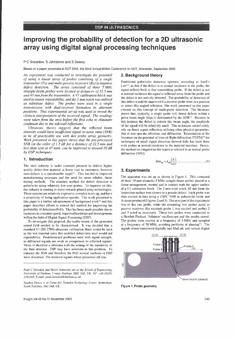
DSP IN ULTRASONICS
Improving the probability of detection for a 2D ultrasonic array using digital signal processing techniques
P C Snowdon, S Johnstone and S Dewey
Based on a paper presented at NDT 2003, the 42nd Annual British Conference on NDT, Worcester, September 2003.
An experiment was conducted to investigate the potential of using a linear array of probes consisting of a single transmitter (Tx) and multi-passive receivers (Rx) to improve defect detection. The array consisted of three 5 MHz straight-beam probes were located at distances of 22.5 mm and 45 mm from the transmitter. A VI calibration block was used to ensure repeatability, and the 2 mm notch was utilised as substitute defect. The probes were used in a single transmission with dual-receiver formation in alternate positions. This experimental set-up was used to reveal the clearest interpretation of the received signal. The readings were taken from the area before the first echo to eliminate confusion due to the sidewall reflections.
Ultrasonic theory suggests that the reflected beam intensity would have insufficient signal-to-noise ratio (SNR) to be of practicable use with this probe array geometry. Work presented in this paper shows that the pre-processed SNR (in the order of 1.5 dB for a distance of 22.5 mm and less than zero at 45 mm), can be improved to around 20 dB by DSP techniques.
1. Introduction The steel industry is under constant pressure to deliver higher quality defect-free material at lower cost to customers; however zero-defects is a questionable target'". This has led to improved manufacturing processes and the need for more reliable, faster testing methods. The standard method for defect detection is pulse/echo using relatively low-cost probes. To improve on this, the industry is tending to move towards phased array technologies. These systems are relatively expensive, complex in set-up, and have a propensity of being application-specific. The work presented in this paper is a further advancement of background work<2> and this paper describes efforts to extend this method for improving the probability of detection (PoD). This has been made possible due to increases in computer speed, improved hardware and developments within the field of Digital Signal Processing (DSP).
To investigate this proposal, the usable extent of the generated sound field needed to be characterised. It was decided that a standard V I (BS 2704) ultrasonic calibration block would be used as the test material since this certified defect-free steel would aid repeatability. Predetermined problems were with signal strength, as diffracted signals are weak in comparison to reflected signals. There is therefore a dilemma with the setting of the sensitivity of the flaw detector. DSP may have solutions to this problem. To enhance the SNR and therefore the PoD several methods of DSP were discussed. The received signals where processed off-line.
Paul C Snowdon and Sherri Johnstone are at the School of Engineering, University of Durham, County Durham, DHI 3LE, UK. Tel: +44 (0)191 3342445; E mail: [email protected]
Stephen Dewey is at Corus pk, Swinden Teclmology Centre, Rolherham, South Yorkshire, S60 3AR, UK.
2. Background theory Traditional pulse/echo detection operates, according to Snell's Law 1 3', in that if the defect is at normal incidence to the probe, the signal reflects back to that transmitting probe. If the defect is not at normal incidence the signal is reflected away from the probe and the defect is not actively detected. The probability of detection of this defect would be improved if a receiver probe were in a position to detect this angled reflection. The work presented in this paper extends on this concept of multi-probe detection. The literature shows that, typically, a single probe will detect defects within a given beam angle (Eqn.l) determined by the SNR ( 4'. Because in this instance the defect is outside this beam angle, the amplitude of the signal will be relatively small. This technique cannot solely rely on direct signal reflection, utilising other physical properties, that of non-specula refection, and diffraction. Examination of the literature on the potential of time-of-flight diffraction (TOFD)' 5 1 for techniques of small signal detection showed little has been done with probes at normal incidence to the material interface. Hence, the method investigated in this report is referred to as normal probe diffraction (NPD).
s « y „ - * « ( | ) (i)
3. Experiments The apparatus was set up as shown in Figure 1. This consisted of three 10 mm-diameter 5 MHz straight-beam probes placed in a linear arrangement, normal and in contact with the upper surface of a V I calibration block. The 2 mm-wide notch, 85 mm from the inspection surface was chosen as a pseudo defect. Each probe was then excited in turn using a USPC 3100 in pulse/echo mode and A-scans produced (Figures 2 and 3). The next part of the experiment was to fire one probe, while the remaining two probes acted as passive receivers (for example probe 1 was excited and probes 2 and 3 acted as receivers). These two probes were connected to a Hewlett Packard 'Infinium' oscilloscope and the results stored. The probes were excited at a frequency of 5 MHz and sampled at a frequency of 50 MHz, avoiding problems of aliasing'61. The signals where transferred digitally into MatLab, and various digital
22.50 . . . 22.50
Probe 1 Probe 3
100 Probe 2
2mm Notch (defect)
Figure 1. Probe geometry
Insight Vol 45 No 11 November 2003 743
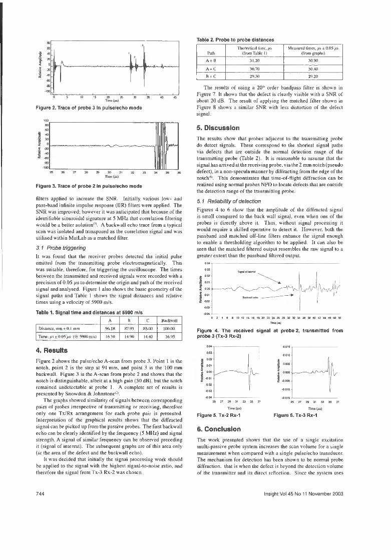
Time (us)
Table 2. Probe to probe distances
Figure 2. Trace of probe 3 in pulse/echo mode
Time (us)
Figure 3. Trace of probe 2 in pulse/echo mode
filters applied to increase the SNR. Initially various low- and pass-band infinite impulse response (IIR) filters were applied. The SNR was improved; however it was anticipated that because of the identifiable sinusoidal signature at 5 MHz that correlation filtering would be a better solution17'. A backwall echo trace from a typical scan was isolated and transposed as the correlation signal and was utilised within MatLab as a matched filter.
3.1 Probe triggering It was found that the receiver probes detected the initial pulse emitted from the transmitting probe electromagnetically. This was suitable, therefore, for triggering the oscilloscope. The times between the transmitted and received signals were recorded with a precision of 0.05 fis to determine the origin and path of the received signal and analysed. Figure l also shows the basic geometry of the signal paths and Table 1 shows the signal distances and relative times using a velocity of 5900 m/s.
Table 1. Signal time and distances at 5900 m/s A B C Backwall
Distance, mm ± 0.1 mm 96.18 87.93 85.00 100.00
Time, lis ± 0.05 lis (cs 5900 m/s) 16.30 14.90 14.40 16.95
4. Results Figure 2 shows the pulse/echo A-scan from probe 3. Point 1 is the notch, point 2 is the step at 91 mm, and point 3 is the 100 mm backwall. Figure 3 is the A-scan from probe 2 and shows that the notch is distinguishable, albeit at a high gain (50 dB). but the notch remained undetectable at probe 1. A complete set of results is presented by Snowdon & Johnstone0'.
The graphs showed similarity of signals between corresponding pairs of probes irrespective of transmitting or receiving, therefore only one Tx/Rx arrangement for each probe pair is presented. Interpretation of the graphical results shows that the diffracted signal can be picked up from the passive probes. The first backwall echo can be clearly identified by the frequency (5 MHz) and signal strength. A signal of similar frequency can be observed preceding it (signal of interest). The subsequent graphs are of this area only (ie the area of the defect and the backwall echo).
It was decided that initially the signal processing work should be applied to the signal with the highest signal-to-noise ratio, and therefore the signal from Tx-3 Rx-2 was chosen.
Path Theoretical time, /<s
(from Table 1) Measured times, /<s ± 0.05 /*s
(from graphs)
A+ B 31.20 30.90
A + ( 30.70 30.40
B + C 29.30 29.20
The results of using a 20* order bandpass filter is shown in Figure 7. It shows that the defect is clearly visible with a SNR of about 20 dB. The result of applying the matched filter shown in Figure 8 shows a similar SNR with less distortion of the defect signal.
5. Discussion The results show that probes adjacent to the transmitting probe do detect signals. These correspond to the shortest signal paths via defects that are outside the normal detection range of the transmitting probe (Table 2). It is reasonable to assume that the signal has arrived at the receiving probe, via the 2 mm notch (pseudo defect), in a non-specula manner by diffracting from the edge of the notch'8'. This demonstrates that time-of-flight diffraction can be realised using normal probes NPD to locate defects that are outside the detection range of the transmitting probe.
5.1 Reliability of detection Figures 4 to 6 show that the amplitude of the diffracted signal is small compared to the back wall signal, even when one of the probes is directly above it. Thus, without signal processing it would require a skilled operative to detect it. However, both the passband and matched off-line filters enhance the signal enough to enable a thresholding algorithm to be applied. It can also be seen that the matched filtered output resembles the raw signal to a greater extent than the passband filtered output.
I 10 12 14 16 18 20 22 24 26 28 30 32 34 36 38 40 42 44 46 48 50 Time (Ms)
Figure 4. The received signal at probe 2, transmitted from probe 3 (Tx-3 Rx-2)
Q 001
26 27 29 31 33
Time (us)
Figure 5. Tx-2 Rx-1
6. Conclusion
00-5
0010
I 0 005
J 0.000
-0 005
-0010
-0.015
25 27 2S 31 33 35 37
Time (us)
Figure 6. Tx-3 Rx-1
The work presented shows that the use of a single excitation multi-passive probe system increases the scan volume for a single measurement when compared with a single pulse/echo transducer. The mechanism for detection has been shown to be normal probe diffraction, that is when the defect is beyond the detection volume of the transmitter and its direct reflection. Since the system uses
744 Insight Vol 45 No 11 November 2003
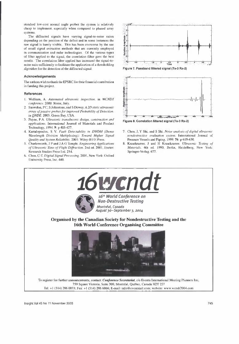
standard low-cost normal angle probes the system is relatively cheap to implement, especially when compared to phased array systems.
The diffracted signals have varying signal-to-noise ratios depending on the position of the defect and in some instances the raw signal is barely visible. This has been overcome by the use of small signal extraction methods that are currently employed in communication and radar technologies. Of the various types of filter applied to the signal, the correlation filter gave the best results. The correlation filter applied has increased the signal-to-noise ratio sufficiently to facilitate the application of a thresholding algorithm for the detection of the diffracted signal.
Acknowledgements The authors wish to thank the EPSRC for their financial contribution in funding this project.
References 1. Wolfram, A. Automated ultrasonic inspection, in WCNDT
conference. 2000. Rome, Italy. 2. Snowdon, P C , S Johnstone, and S Dewey. A 2D static ultrasonic
array of passive probes for improved Probability of Detection. in QNDE. 2003. Green Bay, USA.
3. Payne, P A . Ultrasonic transducers: design, construction and applications. International Journal of Materials and Product Technology, 1994. 9: p 403-427.
4. Kartalopoulos, S V. Fault Detectability in DWDM (Dense Wavelength Division Multiplexing): Toward Higher Signal Quality and System Reliability. 2001: Wiley-IEEE Press.
5. Charlesworth, J P and J A G Temple. Engineering Applications of Ultrasonic Time-of-Flight Diffraction. 2nd ed. 2001, Exeter: Research Studies Press Ltd. 254.
6. Chen, C-T. Digital Signal Processing. 2001, New York: Oxford University Press. Inc. 440.
i6wcndt 16th World Conference on Non-Destructive Testing
Montreal, Canada August30~September3, 2004
Organised by the Canadian Society for Nondestructive Testing and the 16th World Conference Organising Committee
1 1,1
To register for further announcements, contact: Conference Secretariat, c/o Events International Meeting Planners Inc, 759 Square Victoria, Suite 300. Montreal, Quebec, Canada H2Y 2J7
Tel: +1 (514) 286 0855; Fax: +1 (514) 286 6066; E-mail: [email protected]; website: www.wcndt2004.com
n-1 • • 5
T i m e
Figure 7. Passband filtered signal (Tx-3 Rx-2)
<
—JlnM
Sample number*! 50MHz
Figure 8. Correlation filtered signal (Tx-3 Rx-2)
7. Chen, J, Y Shi, and S Shi. Noise analysis of digital ultrasonic nondestructive evaluation system. International Journal of Pressure Vessels and Piping, 1999. 76: p 619-630.
8. Krautkramer, J and H Krautkramer. Ultrasonic Testing of Materials. 4th ed. 1990, Berlin, Heidelberg, New York: Springer-Verlag. 677.
Insight Vol 45 No 11 November 2003 745

Presented at BINDT Conference 2005
Real-Time DSP System for Normal Probe Diffraction Technique
Lei Zhang, Paul C. Snowdon, Sherri Johnstone Affiliation
School of Engineering, University of Durham, County Durham DH1 3LE, UK 0191 3342542
Steve Dewey Corus pic. Swinden Technology Centre, Rotherham, South Yorkshire S60 3AR, UK
Abstract
In steelmaking, on-line defect position and real-time size detection are desired. Many methods have been tried and developed for achieving a reliable cost-effective solution. Ultrasonic detection is commonly used in this field of non-destructive testing (NDT) in the steel industry. Traditional ultrasonic defect detection systems use an array of probes in which each probe pulses and receives sequentially. One new ultrasonic detection technology-Normal Probe Diffraction (NPD) has been proven to enhance the probability of detection for steel testing in the previous research.
In this project, a rapid Digital Signal Processing (DSP) prototype for realising the realtime system is modelled and simulated to implement the NPD technique. A DSP integrated development board is used to implement the NPD algorithm and process the digital signal in real-time. An analog expansion daughterboard is also applied in order to gain a fast digital-to-analogue conversion speed for the desired high frequency pulse signal. Variable frequency and wave shape pulse signals can be used in order to gain the best testing effect. A custom high frequency high voltage power amplifier is also designed to get a good response from the transducers. To remove the randomly distributed background noise that disturbs the recognition of the defect echoes and increase the behaviour of the system, several DSP algorithms such as correlation are applied and different filters including FIR filter and IIR filter can be chosen for experiments as well.
The developed real-time system will help increase the probability of detection of defects in steel billets and produce low-cost system solution for ultrasonic billet inspection in steel industry.
1. Introduction
Various defects such as inclusions, bubbles and cracks can affect the quality of the steel and may cause tremendous waste in the steel industry; therefore the detection and recognition of these defects without destructing the tested object is becoming increasingly significant. In steelmaking, on-line defect position and real-time size detection are desired under the urgent requirement for higher quality products. Many methods have been tried and developed for achieving a reliable cost-effective solution. Ultrasonic detection is commonly used in this field of non-destructive testing (NDT) in the steel industry. Traditional ultrasonic defect detection systems use an array of probes

Presented at BINDT Conference 2005
in which each probe pulses and receives sequentially. One new ultrasonic detection technology-Normal Probe Diffraction (NPD) has been proven to enhance the probability of detection for steel testing in the previous researchIn this work, the necessary realtime system is simulated with software and the corresponding hardware is to be realised and tested to demonstrate the result. In order to gain the best testing effect, a high voltage amplifier is designed for the high frequency output ultrasonic to get a good response from the transducers and gain a better feedback from the tested object. A variable frequency and pulse shape can be completely and flexibly controlled in realtime. To remove the randomly distributed background noise that disturbs the recognition of the defect echoes and increase the behaviour of the system, several Digital Signal Processing (DSP) algorithms are applied and different filters can be chosen for real-time analysis as well.
2. Normal Probe Diffraction
2.1 Background Knowledge
The nature of the project dictates the specific areas of concentrated ultrasonic research, however all areas of wave propagation are to be briefly researched to ensure no potential avenue is overlooked.
The transducer forms the core of all non-destructive ultrasonic inspection procedures, and whether a work-piece can be inspected or not depends upon the acoustic properties they possess. The choice of the correct transducer is therefore indicative for the quality and the reliability of inspection results. Ultrasonic transducers work almost exclusively according to the piezoelectric effect, and there are four fundamental transducer types: Straight beam transducers, Angle beam transducers, Delay line transducers and Twin crystal transducers. In this project, the straight beam transducer is initially required and is dictated by the remit. This type of transducer has one main drawback, in that the poor recognition of near-to-surface discontinuities due to the width of the initial pulse, however in this project it is the core of the material that is of most interest.
Transducers also differ with respect to the size of the active piezoelectric elements, their frequency, bandwidth and the basic design. The selection of bandwidth is essential for achieving certain test results - narrow bandwidth for highly sensitive testing, or broad banded for high resolution testing. The sound field characteristics of a transducer, is generally derived from the diameter and the frequency of the piezoelectric element.
The Near Field is the region in an ultrasonic beam that is subject to variations of intensity due to diffraction effects. It extends from the source of radiation to a point just short of the far field. Diffraction is a particular example of wave interference and is common to all wave motion. Defect detection in the near zone should be avoided unless the characteristics of the probe used are accurately known. Figure 1 shows the near field N, the angle of divergence of ^ and the far field for a typical circular probe.
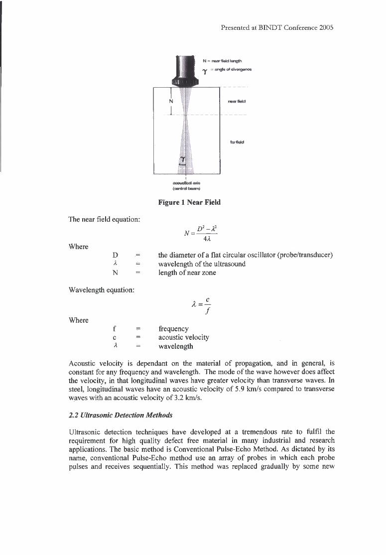
Presented at BINDT Conference 2005
1 rw«H»ld
I
tarMd
(antral
Figure 1 Near Field
The near field equation:
Where D A
N
N = D 2 - A 2
AX
the diameter of a flat circular oscillator (probe/transducer) wavelength of the ultrasound length of near zone
Wavelength equation:
Where
c
k
/
frequency acoustic velocity wavelength
Acoustic velocity is dependant on the material of propagation, and in general, is constant for any frequency and wavelength. The mode of the wave however does affect the velocity, in that longitudinal waves have greater velocity than transverse waves. In steel, longitudinal waves have an acoustic velocity of 5.9 km/s compared to transverse waves with an acoustic velocity of 3.2 km/s.
2.2 Ultrasonic Detection Methods
Ultrasonic detection techniques have developed at a tremendous rate to fulfil the requirement for high quality defect free material in many industrial and research applications. The basic method is Conventional Pulse-Echo Method. As dictated by its name, conventional Pulse-Echo method use an array of probes in which each probe pulses and receives sequentially. This method was replaced gradually by some new
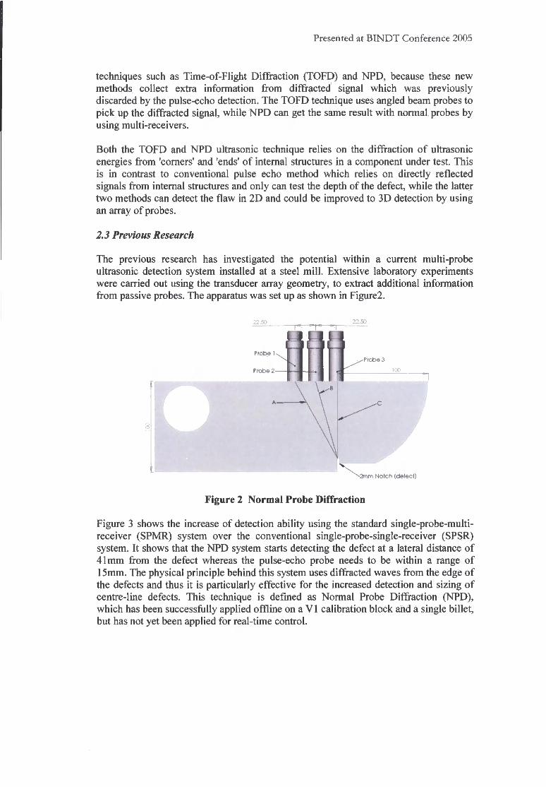
Presented at BINDT Conference 2005
techniques such as Time-of-Flight Diffraction (TOFD) and NPD, because these new methods collect extra information from diffracted signal which was previously discarded by the pulse-echo detection. The TOFD technique uses angled beam probes to pick up the diffracted signal, while NPD can get the same result with normal probes by using multi-receivers.
Both the TOFD and NPD ultrasonic technique relies on the diffraction of ultrasonic energies from 'corners' and 'ends' of internal structures in a component under test. This is in contrast to conventional pulse echo method which relies on directly reflected signals from internal structures and only can test the depth of the defect, while the latter two methods can detect the flaw in 2D and could be improved to 3D detection by using an array of probes.
2.3 Previous Research
The previous research has investigated the potential within a current multi-probe ultrasonic detection system installed at a steel mill. Extensive laboratory experiments were carried out using the transducer array geometry, to extract additional information from passive probes. The apparatus was set up as shown in Figure2.
Figure 3 shows the increase of detection ability using the standard single-probe-multi-receiver (SPMR) system over the conventional single-probe-single-receiver (SPSR) system. It shows that the NPD system starts detecting the defect at a lateral distance of 41mm from the defect whereas the pulse-echo probe needs to be within a range of 15mm. The physical principle behind this system uses diffracted waves from the edge of the defects and thus it is particularly effective for the increased detection and sizing of centre-line defects. This technique is defined as Normal Probe Diffraction (NPD), which has been successfully applied offline on a V I calibration block and a single billet, but has not yet been applied for real-time control.
22.50 m Probe 3
Probe 2
2mm Notch (defectl
Figure 2 Normal Probe Diffraction
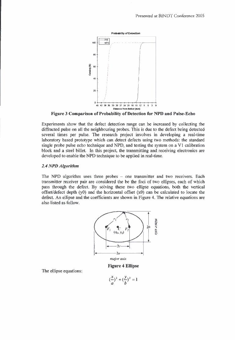
Presented at BINDT Conference 2005
Probability of Detection
100
PIE
N P D
T 80
* 60
40
20
0 1 45 42 39 36 33 30 27 24 21 16 15 12 9 6 3 0
Distance from Defect (mm)
Figure 3 Comparison of Probability of Detection for NPD and Pulse-Echo
Experiments show that the defect detection range can be increased by collecting the diffracted pulse on all the neighbouring probes. This is due to the defect being detected several times per pulse. The research project involves in developing a real-time laboratory based prototype which can detect defects using two methods: the standard single probe pulse echo technique and NPD, and testing the system on a V I calibration block and a steel billet. In this project, the transmitting and receiving electronics are developed to enable the NPD technique to be applied in real-time.
2.4 NPD Algorithm
The NPD algorithm uses three probes - one transmitter and two receivers. Each transmitter receiver pair are considered the be the foci of two ellipses, each of which pass through the defect. By solving these two ellipse equations, both the vertical offset/defect depth (yO) and the horizontal offset (xO) can be calculated to locate the defect. An ellipse and the coefficients are shown in Figure 4. The relative equations are also listed as follow.
lb ^ F\ T* (J*>>h)
2c
major axis
Figure 4 Ellipse The ellipse equations:
( - ) 2 + # 2 = l a

Presented at BINDT Conference 2005
a2=b2+c2
r, + r2 =2* a
Table 1. Transmit Distance and Time
Path Distance (mm) Time (us) A 96.18 16.3 B 87.93 14.9 C 85 14.4
Backwall 100 16.95 Note: d = v*t;v = 5900 m/s
Table 1 gives out the tested distances of path A, B and C in millimetre, with the theoretical time in microsecond calculated from the distances with the velocity of 5900m/s. The experiment setups and ellipse graphs for double probes and triple probes are shown separately in Figure 5 and Figure 6. The distance between each two probes is set to 22.5mm and the depth of the defect (notch) is 85mm (2).
For double probe NPD, probe 1 transmits signal and then receives the diffracted signal, so the first path is 2 x B and forms a circle whose radius (R) is B. The second path is formed by transmitter probe 1 and receiver probe 2, making an ellipse whose major axis equals to B plus C.
Similarly, for triple probes NPD, probe 1 only transmits signal and forms two ellipses with receiver probe 2 and receiver probe 3. The major axes for each are A plus B and A plus C separately.
1 2 1 2 3 Tx - Transmitter R1 - Receiver 1 R2- Receiver 2 31
B\ C A v =2' B
A+B V =B + C Q*V=A+C
Doubk ProWti N30 Tr.pla Probes
RX R1ITR2 Tx !3 E ps.
-
: i r 153 — I I
•
70 •
-1! t l l ipsel
i T.M02 : I •a x i ICC 40 • i -•100 •- •20
Figure 6 Triple Probes Scheme Figure 5 Double Probes Scheme 2.5 NPD Simulation Model

Presented at BINDT Conference 2005
Simulink Models have been built to simulate the Pulse-echo, Double Probes NPD and Triple Probes NPD algorithms. Figure 7 shows that by calculating the time delay of two transmit paths - t l and t2, the algorithm can locate the pseudo defect in 2 dimensions. These blocks can be called as individual functions during the idle time in real-time data acquisition.
31.2 2 2 ^ 1 • I t1 fus )A+B
xO 3p 30.7 t2 NPD_Tr ip leProbes
1
t2(us)A+C 84.95 y£>
5900
yO 3p v(m/s) Mat lab E m b e d d e d Funct ion
f 1 .:• Doub leProbes
i 29.8 • I 22.68
t1 fus12 'B 29.3 ub leProbes X0 2p
84 .94 t2(us) B+C
yO_2p Mat lab E m b e d d e d Func t ion l
•
28.8
84.96 t fus)2*C PulseEoho
yO PE
Mat lab E m b e d d e d Funct ion2
Figure 7 NPD Algorithm Simulation Model
3. DSP System
3.1 Hardware
• TMS320C6713 DSK • AED 330 Analog Expansion Daughterboard • High Voltage High Frequency Amplifier •
3.2Software • Matlab and Simulink • Code Composer Studio

Presented at BINDT Conference 2005
3.3 System Architecture Figure 8 depicts the architecture of a rapid Digital Signal Processing (DSP) prototype for the real-time testing system. Firstly a Simulink model is built using the MATLAB
A Rapid Real-Time DSP Prototype
Matlab System mode g . ^ . ^
ime
Build project AED-330
I Daughterboard
Code Composer Studio
Load program TI C6713 DSK
Figure 8 A Rapid Real-Time DSP Prototype
Embedded Target for DSP and DSP blockset which enable the rapid prototyping of realtime software for the TMS320C6713 floating-point processor and generates efficient code for the processor directly from the Simulink model. The generated code is readable and editable for manual optimization. The Embedded Target automates the creation of a link to the Integrated Development Environment, IDE, which provides board support software for the DSK board. It then invokes the compiler and linker to create a DSP executable file and finally downloads the executable to the DSK board and sets it running for real-time algorithm evaluation. An AED-330 analogue expansion daughterboard is mounted on the DSK to gain high speed digital to analogue and analogue to digital conversion for the desired high frequency pulse signal. Variable frequency and wave shape pulse signals can be used in order to gain the optimum testing conditions. A high voltage power amplifier is also designed to get a good response from the transducers (3). To remove the randomly distributed background noise that disturbs the recognition of the defect echoes and increase the behaviour of the system, several DSP algorithms such as correlation are applied and different filters including FIR filter and IIR filter can be chosen for real-time analysis as well (4).
4. Conclusion
The real-time system leads to a great improvement in verifying and realising NPD. Much information discarded by conventional test methods of ultrasonic billet inspection can be used due to modern advances in DSP. Therefore, the system not only improves the test integrity and sensitivity, but also makes the experiment data easy to acquire, analyze and visualise. After the successful simulation of the signal-channel system, a probe array based on the geometry in a typical ultrasonic defect detection system is being built and driven using sequential transmitter and parallel receiver processing units. The electronic hardware to achieve this goal has been designed and constructed.

Presented at BINDT Conference 2005
References
1. P C Snowdon, S Johnstone, S Dewey, (2003), A 2D static ultrasonic array of passive probes for improved Probability of Detection, Nondestructive Testing and Evaluation, 19(3), pp. 111-120
2. PC Snowdon, S Johnstone, S Dewey, (2003), Improving the probability of detection for a 2D ultrasonic array using digital signal processing techniques, Insight 45(11)
3. R. L. Tutwiler, S Madhavan, K. V. Mahajan, (1999), Design of a Test System to Characterize Very High-Frequency Ultrasound Transducer Arrays, SPIE 3664(182)
4. R. Venteris, (2002) Exploration of DSP architectures in ultrasonic measurement application, Ultragarsas Journal 42(1)

Presented at IoM3 Conference 2005
Normal Probe Diffraction - Improving the capability of industrial ultrasonic probe arrays
Lei Zhang, Sherri Johnstone, Paul C. Snowdon, School of Engineering, University of Durham, DH1 3LE Steve Dewey, STC, Rotherham, Corus
Abstract
In bloom and billet mills, on-line defect detection systems exist, in which each probe is sequentially used to produce a radio frequency pulse, which is then reflected from the defect and detected by the same probe. The work carried out in this project shows that extra information can be obtained about the defect i f the diffracted signal is also collected by neighbouring probes and digital signal processing algorithms are applied to improve the signal to noise ratio. This technique is similar to time-of-flight diffraction, but does not require angled probes, and is thus referred to as normal probe diffraction, NPD. The advantage of this method is that it is possible to apply it in real-time thus giving the possibility of improved on-line defect detection, sizing and orientation. This paper describes the physical principles of NPD together with the hardware and software development required to implement the system in real time. The results on a simulated defect show that it can be detected from a distance of 41mm using NPD as opposed to 15mm with the sequential single probe pulse-echo method.
Key words: Normal Probe Diffraction (NPD), Digital Signal Processing (DSP), real-time, ultrasonic detection, non-destructive testing (NDT)
1. Introduction
The defects of steel mainly include inclusions, bubbles and cracks, all of which can affect the quality of the steel to some degree, therefore their detection and recognition is becoming increasingly significant, due to the customer lead demand for higher quality products. In steel making, on-line defect position and real-time size detection are desired. Many methods have been tried and developed for achieving a reliable cost-effective solution. Ultrasonic detection is commonly used in this field of non-destructive testing (NDT) in the steel industry. Traditional ultrasonic defect detection systems use an array of probes in which each probe pulses and receives sequentially. One new ultrasonic detection technology-Normal Probe diffraction (NPD) has been proven to enhance the probability of detection for steel testing in the previous researchfl]. In this work, the necessary real-time system is simulated with software and the corresponding hardware is to be realised and tested to demonstrate the result. In order to gain the best testing effect, an ultrasonic pulser is designed to generate a variable frequency and pulse shape, which can be completely and flexibly controlled in real-time. A high voltage power amplifier is also designed to get a good response from the transducers. To remove the randomly distributed background noise that disturbs the recognition of the defect echoes and increase the behaviour of the system, several Digital Signal Processing (DSP) algorithms are applied and different
filters can be chosen for real-time analysis as well. The developed real-time system will help increase the probability of detection of defects in steel billets and produce low-cost system solution for ultrasonic billet inspection in steel industry.
2. Previous Research
The previous research has investigated the potential within a current multi-probe ultrasonic detection system installed at a steel mill. Extensive laboratory experiments were carried out using the transducer array geometry, to extract additional information from passive probes. The apparatus was set up as shown in Figurel [2].
2250 • 1
41 Piobe 1 P r o b » 3
Probe 2
^ ^ S m m N o t c h ( d e f e c t )
Figure 1 Probe Geometry
1
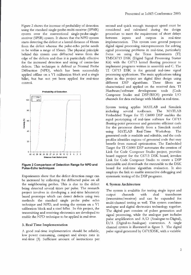
Presented at IoM3 Conference 2005
Figure 2 shows the increase of probability of detection using the standard single-probe-multi-receiver (SPMR) system over the conventional single-probe-single-receiver (SPSR) system. I t shows that the NPD system starts detecting the defect at a lateral distance of 41mm from the defect whereas the pulse-echo probe needs to be within a range of 15mm. The physical principle behind this system uses diffracted waves from the edge of the defects and thus it is particularly effective for the increased detection and sizing of centre-line defects. This technique is defined as Normal Probe Diffraction (NPD), which has been successfully applied offline on a V I calibration block and a single billet, but has not yet been applied for real-time control.
Probability of Detection
45 42 39 36 33 30 27 24 21 18 15 12 9 6 Distance from Defect (mm)
Figure 2 Comparison of Detection Range for NPD and Pulse-Echo techniques
Experiments show that the defect detection range can be increased by collecting the diffracted pulse on all the neighbouring probes. This is due to the defect being detected several times per pulse. The research project involves in developing a real-time laboratory based prototype which can detect defects using two methods: the standard single probe pulse echo technique and NPD, and testing the system on a V I calibration block and a steel billet. In this project, the transmitting and receiving electronics are developed to enable the NPD technique to be applied in real-time.
3. Real Time Implementation
A good real-time implementation should be reliable, low power consuming, compact and always runs in real-time [3]. Sufficient amount of instructions per
second and quick enough transport speed must be considered and calculated during the design procedure to meet the requirement of short delays between inputs and outputs in real-time implementation. This system uses general purpose digital signal processing microprocessors for solving signal processing problems in real-time, particularly focus on using the Texas Instruments (TI) TMSC6713 DSK (Digital Signal Processing Starter Kit) with the C6713 kernel floating processor to implement programs written in assembly and C. The T I C6713 DSK is for general real-time signal processing applications. The main applications taking place in this project are digital filter design using different DSP algorithms. These filters are characterized and applied on the received data. T I Hardware/software development tools (Code Composer Studio and DSP/BIOS) provide I / O channels for data exchange with Matlab in real-time.
System testing applies MATLAB and Simulink including several toolboxes. The MATLAB Embedded Target for T I C6000 DSP enables the rapid prototyping of real-time software for C6713 floating-point processor and generates efficient code for the processor directly from a Simulink model using MATLAB Real-Time Workshop. The generated code is readable and editable, and the code profiler identifies regions of generated code that may benefit from manual optimisation. The Embedded Target for T I C6000 DSP automates the creation of Link for Code Composer Studio project, provides board support for the C6713 DSK board, invokes Link for Code Composer Studio to create a DSP executable and downloads the executable to the DSK board for real-time algorithm evaluation. It also employs the link to enable interactive debugging and systematic testing of the DSP programs.
4. System Architecture
The system is available for testing single input and output channels with dual transducers (transmitter/receiver) and can be expanded for multi-channel testing as well. This system combines analogue and digital electronics technology together. The digital part consists of pulser generation and signal processing, while the analogue part includes pulse amplification and A / D (Analogue-to-Digital), D / A (Digital-to-Analogue) conversion. A single channel system is illustrated in figure 3. The digital pulse signal generated by C6713DSK, with a variable
2
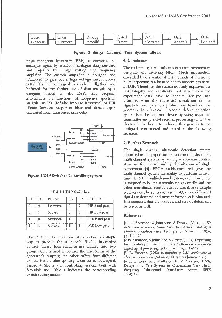
Presented at IoM3 Conference 2005
Pulse D / A Analog Tested A m n l i f i T a rm*t H A / D Data Data
A nalircic T r\rr anrl
Figure 3 Single Channel Test System Block
pulse repetition frequency (PRF), is converted to analogue signal by AED330 analogue daughter-card and amplified by a high voltage high frequency amplifier. The custom ampKfier is designed and fabricated to give out a high voltage output above 200V. The echoed signal is received, digitised and buffered for the further use of data analysis by a program loaded on the DSK. The program implements the functions of frequency spectrum analysis, an IIR (Infinite Impulse Response) or FIR (Finite Impulse Response) filter and defect depth calculated from transceiver time delay.
Trigger ,
swo
SW1
S W 2
SW3
hign sine square sawtootn custom
logical operatoi
00 h igh
01
10 lew 11
• F 2
logical operator Filters
Figure 4 DIP Switches Controlling system
Tablel DIP Switches
DO D l PULSE D 2 D3 F I L T E R
0 0 Sinewave 0 0 I IR Band pass
0 1 Square 0 1 I I R L o w pass
1 0 Sawtooth 1 0 FIR Band pass
1 1 Custom 1 1 FIR L o w pass
The 6713DSK includes four DIP switches as a simple way to provide the user with flexible interactive control. These four switches are divided into two groups. One is used to control the waveforms of the generator's outputs; the other offers four different choices for the filter applying upon the echoed signal. Figure 4 Shows the controlling system built with Simulink and Table 1 indicates the corresponding switch setting modes.
6. Conclusion
T h e real-time system leads to a great i m p r o v e m e n t i n v e r i f y i n g and realising N P D . M u c h i n f o r m a t i o n discarded by convent ional test methods o f ultrasonic bil let inspection can be used due to mode rn advances i n DSP. Therefore , the system n o t only improves the test integri ty and sensitivity, bu t also makes the experiment data easy to acquire, analyze and visualise. A f t e r the successful s imulat ion o f the signal-channel system, a probe array based o n the • geometry i n a typical ultrasonic defect detection system is to be bui l t and dr iven by using sequential transmitter and parallel receiver processing units. T h e electronic hardware to achieve this goal is to be designed, constructed and tested i n the f o l l o w i n g research.
7. Further Research
T h e single channel ultrasonic detection system discussed i n this paper can be replicated to develop a mul t i -channel system by adding a sof tware con t ro l structure f o r con t ro l and synchronizat ion o f single componen t [4]. F P G A architecture w i l l give the mul t i -channel system the ability to p e r f o r m i n real-t ime. I n N P D mult i -channel system, each transducer is assigned to be the transmitter sequentially and the other transducers receive echoed signal. A s mul t ip le receivers can be set up to test i n 3 D , more d i f f r ac ted signal are detected and more i n f o r m a t i o n is obtained. I t is expected that the pos i t ion and size o f defect can be tested as wel l .
References
[ I ] PC Snowdon, S Johnstone, S Dewey, (2003), A 2D static ultrasonic array of passive probes for improved Probability of Detection, Nondestructive Testing and Evaluation, 19(3), pp. 111-120 [2]PC Snowdon, S Johnstone, S Dewey, (2003), Improving the probability o f detection for a 2 D ultrasonic array using digital signal processing techniques, Insight 45(11) [3] R Venteris, (2002) Exploration of DSP architectures in ultrasonic measurement application, Ultragarsas Journal 42(1) [4] R. L . Tutwiler, S Madhavan, K . V . Mahajan, (1999), Design o f a Test System to Characterize Very High-Frequency Ultrasound Transducer Arrays, SPIE 3664(182)
3
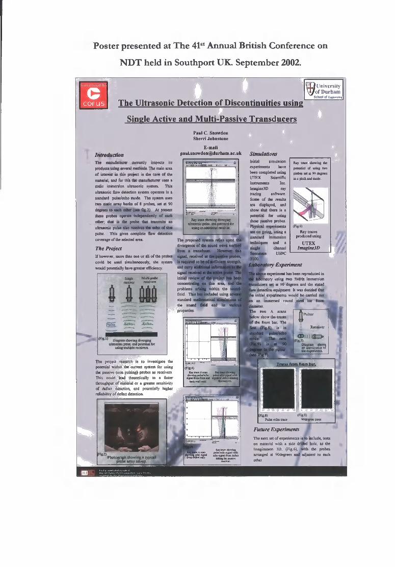
Poster presented at The 41st Annual British Conference on
NDT held in Southport UK. September 2002.
S I H H I M M id In
I O I I I S The Ultrasonic Detection of Discontinuities using
Single Active and Multi-Passive Transducers Paul C . Snowdon Sherri Johnstone
ED University \J/of Durham
School of B -
Introduction The manufacturer currently inspects its products using several methods. The main area of interest in this project is the core of the material, and for this the manufacturer uses a static immersion ultrasonic system. This ultrasonic flaw detection system operates in a standard pulse/echo mode. The system uses two static array banks of 8 probes, set at 90 degrees to each other (see fig.2). At present these probes operate independently of each other, that is the probe that transmits an ultrasonic pulse also receives the echo of that pulse. This gives complete flaw detection coverage of the selected area
The Project If however, more than one or all of the probes could be used simultaneously, the system would potentially have greater efficiency.
Single receiver
Multi probe receivers
(Fig.1) Diagram showing diverging ultrasonic pulse, and potential for
using multiple receivers.
The project research is to investigate the potential within the current system for using the passive (non pulsing) probes as receivers. This could lead theoretically to a faster throughput of material or a greater sensitivity of defect detection, and potentially higher reliability of defect detection.
E-mail [email protected]
Ray (race showing diverging ultrasonic pulse, and potential for
using an additional receiver
Ray trace showing the potential of using two probes set at 90 degrees in a pitch and mode.
The proposed system relies upon the divergence of the sound wave emitted from a transducer. However this signal, received at the passive probes, is required to be of •ufficieol strength, and carry additional mformatior signal received at the active probe The initial review of the project has been concentrating on this area, and the problems arising within the agalH field This has included using : standard mathematical the sound field and its properties.
Fig 2) Photograph showing a ty
probe array set-up
fcjStS
lFig.4) b y
ligral from frcrt iod m bbi -wi l l only
Simulations Initial simulation experiments have been completed using UTEX Scientific Instruments Inc. Imagine3D ray tracing software. Some of the results are displayed, and show that there is a potential for using these passive probes. Physical experiments are on going, using a standard immersion techniques and a single channel Socomate USPC 3JO0.
Laboratory Experiment t experiment has been reproduced in story using two 5MHz immersion
lucers set at 90 degrees and the stated detection equipment. It was decided that
initial experiments would be carried out an immersed round steel bar
two A scans tow show the traces the 8mm bar. The
•st (Fig.S), is in standard pulse/echo mode The next
(Fig.6) Ray traces
produced using
U T E X Imagined D
Pulsar
CD
Diagram show s III apprvnini.ili .il 01 ihe experiment
Traces from 8mm bar
into Wdegrce trace PIIINC echo kpjee
Future Experiments The next set of experiments is to include, tests on material with a side drilled hole, as the Imagination 3D, (Fig 6), Jrith the probes arranged at 90degrees and adjacent to each other.
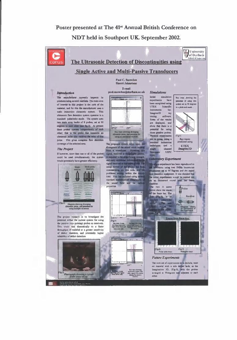
Poster presented at The 41st Annual British Conference on
NDT held in Southport UK. September 2002.
1 ersity r h a m
ScblMll Of 1 neili..rllis
The Ultrasonic Detection of Discontinuities using
Single Active and Multi-Passive Transducers
Introduction The manufacturer currently inspects its products using several methods. The main area of interest in this project is the core of the material, and for this the manufacturer uses a static immersion ultrasonic system. This ultrasonic flaw detection system operates in a standard pulse/echo mode. The system uses two static array banks of 8 probes, set at 90 degrees to each other (see fig.2). At present these probes operate independently of each other, that is the probe that transmits an ultrasonic pulse also receives the echo of that pulse. This gives complete flaw detection coverage of the selected area
The Project If however, more than one or all of the probes could be used simultaneously, the system would potentially have greater efficiency
Mulu probe
6 6 (Fig-D Diagram showing diverging
ultrasonic pulse, and potential for using mutuple receivers
The project research is to investigate the potential within the current system for using the passive (non pulsing) probes as receivers. This could lead theoretically to a faster throughput of material or a greater sensitivity of defect detection, and potentially higher reliability of defect detection.
Paul C . Snowdon Sherri Johnstone
E-mail [email protected]
Ray trace showing diverging ultrasonic pulse, and potential for
using an additional receiver
Ray trace showing the
potential of using two
probes set at 90 degrees
in a pitch and mode.
The proposed system relies upon the divergence of the sound wave emitted from a transducer. However this signal, received at the passive probes, is required to be of sufficient strength, and carry additional inforn signal received at the a c i initial review of the project has been concentrating on this area, and the problems arising within the s^^^H field This hu included using ; standard mathematical the sound field and properties.
Simulations Initial simulation experiments have been completed using UTEX Scientific Instruments Inc. Imagined D ray tracing software. Some of the results are displayed, and show that there is a potential for using these passive probes. Physical experiments are on going, using a standard immersion techniques and a single channel Socomme USPC 3100.jK|
Laboratory Experiment ^ ^ B n experiment has been reproduced in Wm htroratory using two 5MHz immersion pransducers set at 90 degrees and the stated
w detection equipment. It was decided that « initial experiments would be carried out
i immersed round steel bar
(Fig.6) Ray traces
produced using U T E X
Imagine3D
two A scans low show the traces the 8mm bar. The
(Fig.§j, is in standard pulse/echo mode The next
Photograph showing a probe array set-up
(Fig-4) e»y (race A
fit I M i:.̂ Uil-»all only
Traces from 8mm bar,
Pulsar
Receiver
Diagram show s in approxunalioa o f ibe experiment
lFig-9) Pulse echo trace 90degrce trace
Future Experiments The next set of experiments is to include, tests on material with a side drilled bole, as the Imagination 3D, (Fig 6), fcith the probes arranged at 90degrees and adjacent to each other. i ,
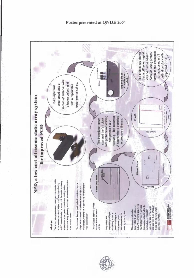
Poster presented at Q N D E 2004
(<*) < M * | » , i
S I * 1