Page 1 of 12

Establishing Meaningful Expectations for Test Performance via Invariant Latent Standards

Greg Hurtz & Ross Brown PSI Services LLC

Presented at the Annual Meeting of the National Council on Measurement in Education Chicago, Illinois, April 2015

Abstract In applied measurement contexts, both test-takers and decision-makers need to comprehend expectations regarding test-taker performance. Setting latent standards that are invariant to specific test content helps to define such expectations across key competence levels. We demonstrate this process, and compare quantitative methods for setting latent standards from standard setting ratings. Introduction In applied measurement contexts, especially high-stakes environments, both test-takers and decision-makers need to comprehend expectations regarding sufficient test-taker performance. To say an assessment program has established “meaningful expectations” is to say that test-takers and those who prepare them know what is expected of them as they prepare for the test, and that decision-makers know where to set the bar on a particular test form to best match those same expectations. These questions are generally asked in reference to performance on an observed test, but they are best answered in reference to the latent competence continuum that underlies test performance. This distinction is made, either implicitly or explicitly, in some standard setting methodologies—but the importance of distinguishing the latent standard from the observed cutscore is not always recognized. The focus of this paper is to emphasize the importance of this distinction, demonstrate its relation to an emerging theme of using construct maps in standard setting to help communicate performance expectations, and review and compare methods for identifying the latent competence thresholds from standard-setting ratings. Invariant Latent Standards vs. Observed Test Cutscores

Performance cutscores on a test are manifestations of underlying thresholds along a latent competence continuum, as depicted in Figure 1. Competence (horizontal axis) is a property of people, not items or tests. The latent threshold lies along this continuum and defines the point at which a person’s competence is sufficient to achieve the objectives of the measurement process—for example, the point beyond which it is expected that a person can practice in the domains covered by the test without harming the public, or multiple points at which different letter grades should be assigned to test performance. But the levels of competence along the latent continuum are independent of – or invariant to – the content of any particular test or set of alternative test forms. This distinction, represented by the horizontal versus vertical axes in Figure 1, is crucial but sometimes given only superficial attention.

Lord and Novick (1968) identified invariance as an ideal condition for item response models. Invariance essentially means that person properties and item/test properties are independent of one another: Item parameters do not vary across different groups of people, and person parameters do not vary across different groups of items. Invariance generally does not hold for classical test theory methods but is an important feature of Rasch and IRT models (Engelhard, 2013; Hambleton, Swaminathan, & Rogers, 1991; Lord & Novick, 1968).

Here we use the phrase “invariant latent standards” in reference to performance level thresholds that are identified along the latent continuum, which can subsequently be applied to any test comprised of items calibrated within the same frame of reference, such as items in the same bank. The latent standard is invariant to the specific content on the items used in the process of establishing the standard, and invariant to any particular sample of test-takers on which item parameters were estimated, and the goal is for it to also be

Page 2 of 12

invariant to any particular sample of subject matter experts used in the standard setting process. Establishing invariant latent standards creates an efficient and reliable means of setting consistent performance standards across all alternate test forms tied to the same latent scale. Once the standards are set, they can be applied to many different alternate forms without the need to conduct separate standard-setting studies for each form. This is even true for items that have never been rated in a standard setting process but have been calibrated to the same scale as those items that have been rated.

Figure 1:

While this general notion of applying the same standard across alternate forms is, admittedly, routine for many practitioners in the test development field who use Rasch or IRT methods, it is common among those using classical test theory methods to spend extensive amounts of time, money, and resources on standard setting workshops for every new form or cycle of alternative forms in order to establish (hopefully) equivalent cutoff scores. Hurtz, Muh, Pierce, and Hertz (2012) argued that when shifting the focus of standard setting to the latent continuum (as opposed to the observed cutoff score), it becomes clear that the practice of running separate workshops for every form is unnecessarily costly, and even worse it can increase the chances of shifting standards across forms. They argued that focusing on the latent scale provides a stronger theoretical basis for standard setting across alternate forms, due largely to maintaining constant standards across the forms. Of course, this assumes that items are calibrated in a Rasch or IRT frame of reference1.

Wyse (2013) recently articulated the use of construct maps, a common component of Rasch measurement (e.g., Engelhard, 2013; Wilson, 2005), in the standard setting realm. Perie (2008) also discussed the use of IRT-calibrated items falling within each defined performance level as way of adding detail to the definition of each performance level. The notion of invariant latent standards is in line with these procedures and recommendations, as they define the critical thresholds along the continuum at which performance-level decisions are made about individuals. Consult Perie (2008) for an extensive discussion of performance-level descriptors, and Wyse (2013) for a thorough articulation of defining construct maps for standard setting purposes. Here our primary focus is identifying the cutoff score thresholds along the latent continuum of a construct map that are invariant to any particular sampling of items from the test’s content domain. 1 Even if this is not the case, standard-setting ratings can be equated across forms to maintain equivalent observed-score standards (Norcini, 1990; Norcini & Shea, 1992), making recurring separate workshops impractical and probably unnecessary. As Norcini and Shea (1997) stated, “…it is unrealistic and perhaps unreasonable to ask experts to devote several days of their time to a process that will produce a result that is substantively indistinguishable from the result of a briefer, but still rigorous process” (p. 44).

Form A

Form B

Form A Cutscore

Form B Cutscore

Page 3 of 12

Identifying the Latent Standards from Angoff Ratings A number of methods have been derived for determining performance standards on the latent Rasch or IRT scale. For example, the Bookmark (Lewis et al., 1996) and Objective Standard Setting (Stone, 2001) methods are aimed directly at identifying the latent threshold. The Angoff method, as commonly applied, is only indirectly related to the latent scale inasmuch as raters can conceptualize minimum competence and translate it into a probability estimate. However, these judgment-based estimates can be analyzed in conjunction with Rasch/IRT-based probability estimates from their item characteristics curves (ICC) to help identify the threshold underlying ratings (Hurtz, Jones, & Jones, 2008; Hurtz et al., 2012; Kane, 1987) and to evaluate rater consistency with actual item properties as displayed in the ICCs (Hurtz & Jones, 2009; van der Linden, 1982).

Kane (1987) outlined several methods of identifying the latent standard, θ*, from Angoff-type probability estimates—some that operate at the individual item level using ICCs, as depicted in the left panel of Figure 2, and others that operate at the test level using test characteristics curves (TCCs) as depicted in the right panel of Figure 2. He also developed variations on these methods that involve weights accounting for rater agreement and conditional item slopes at θ*. Using the conditional item slopes at θ*gives more weight to items that provide their maximum information at cutscore, in attempt to align Angoff ratings (which are sometimes criticized as being “pulled from thin air”) with empirically estimated item properties when deriving the θ*standard. Using rater agreement in the derivation of weights gives more weight to items on which a panel of experts shows less variance in ratings. Assuming agreement is tantamount to accuracy, this factor makes sense; however, Hurtz et al. (2008) cautioned that in practice rater agreement may arise from a number of factors that run counter to accuracy, such as social influence effects or shared heuristics or biases that produce artificially lower variance on some items compared to others. We speculate that differences in rater variance are more idiosyncratic than differences in rater means within different expert panels, and that using rater variance in the derivation of latent standards might therefore work against the generalizability (and invariance) of the standards across rater panels.

Figure 2: Deriving Latent Standards (θ*) from Angoff Ratings via ICCs (left) and the TCC (right)

To demonstrate methods for deriving latent standards from observed Angoff ratings, we use archival

data from an associate level exam for a pre-licensure program sponsored by a private, non-profit college. Angoff ratings were made on 88 unique items from two alternate forms (some are included on both forms as anchors), at four performance levels corresponding to recommended letter grades (A, B, C, and D), which were labeled “Highly Competent,” “Competent,” “Marginally Competent,” and “Weak.” Prior to providing ratings, raters discussed and modified, if needed, the performance level definitions to calibrate the raters on

Page 4 of 12

their conceptions of competence at each level. They were then trained on the Angoff rating process and went through multiple rounds of ratings and discussion until they felt comfortable with the process. They then rated the remaining items and nominated items they had difficulty with for discussion with the group. Their final ratings were recorded and are analyzed in this paper. While all items had been pre-calibrated through pre-testing in the 3-parameter IRT model, it was not standard practice at the time these archival data were recorded for this information to be used in the standard setting process, so raters did not have access to any item performance data. The correlation between ratings and item b values were -0.49, -0.52, -0.54, and -0.56 at the A, B, C, and D performance thresholds.

Preliminary analyses. Prior to exploring different strategies for deriving θ* we performed an item × rater × grade generalizability theory analysis on both the raw ratings and the ratings converted to the latent scale through the items’ ICCs. This conversion process can be conceptualized as finding each rater’s probability estimates for each item along the item’s ICC, and recording the corresponding θ as the equivalent value. Kane (1987) recommended running a generalizability theory analysis on the converted ratings in order to understand the sources of variance impacting θ* and perhaps guide the design of improvements to study design, such as sampling more raters. We ran the analysis on raw ratings as well in order to compare the effects of the conversion process on relative amounts of variance explained by each source both before and after the conversion. This comparison is summarized in Figure 3.

Figure 3:

For interpretation of Figure 3, note first that variance in ratings due to items and grades are good

sources of variance. Ratings should differentiate item difficulties, and ratings should also differentiate performance levels. Together, items and grades accounted for 73% of the variance in raw ratings and 71% of the variance in converted ratings, but the relative portions differed from pre- to post-conversion. For raw ratings, items accounted for a much smaller portion of variance than grade levels (9% vs. 64%) while after conversion through ICCs to the latent scale these percentages were approximately equal (35% vs. 36%). This finding in conjunction with the fairly strong correlations between ratings and item b values reported earlier suggests that raters did a good job of judging the rank order of item difficulties in most cases, but the differences in magnitudes of those differences were constrained in the raw ratings. Aligning ratings with actual item properties through the ICCs spread out the item difficulties in accordance with properties discovered through the separate IRT calibration of items.

73% 71%

26% 19%

1% 11%

Page 5 of 12

The increase in the item × grade interaction component from raw ratings (1%) to converted ratings (11%) may seem troubling at first, as this component indexes changes in the rank ordering of rated item difficulties across grade levels. The trivial 1% in raw ratings suggests that raters did not change rank orders of item difficulties from one grade level to the next. The increase in this component when ICCs were brought into the process is a function of the fact that the ICCs are not parallel in the 3-parameter IRT model. Differing item slopes caused rank orders of item difficulties to differ in the upper versus lower range of the latent continuum, and the addition of the c parameter to account for guessing among low-ability test-takers further exaggerated these differences at the lower end of the continuum. Thus, the increase in this component is fully expected as ratings were aligned to the ICCs that themselves differed in rank ordering of item difficulties at different points along the continuum. Note that if the exam had been calibrated in the 2-parameter IRT model these differences would likely have been smaller, and if the 1-parameter IRT model or the Rasch model were used the ICCs would have been parallel and the I × G component would not be expected to increase from raw to converted ratings.

Figure 4 demonstrates the influence of nonparallel ICCs on the I × G component by reporting the relative results of re-running the analysis for each pairwise comparison of grade levels. The I × G interaction component was largest for those contrasts involving the D performance threshold, which was closest to the lower end of the continuum where the c parameters exaggerated the differing rank orders of items in comparison to the upper end of the continuum. As would be expected, the largest interaction occurred for the contrast between A and D thresholds (19%) followed by the contrast between B and D (17%) and then the contrast between C and D (12%). The A-C contrast was also 12%, followed by B-C (6%) and A-B (4%). Adjacent categories in the mid to upper end of the continuum showed the least change in rank orders, as the ICCs tend to be closer to parallel in these regions.

Figure 4:

Finally, it is noteworthy in Figure 3 that each source of error variance involving raters – the main effect

of raters and the various interactions involving raters – was reduced after conversion to the latent scale. Overall the variance accounted for by the set of rater error components dropped from 26% in the raw ratings to 19% in the converted ratings. This again suggests that using raw ratings in conjunction with item properties contained in the ICCs helped resolve some of the rater inconsistencies in raw ratings. Most noteworthy was

Page 6 of 12

the reduction of the rater × item error component, indexing inconsistencies across raters in rank orders of item difficulties, from 12% to 9%.

Some attention (e.g., Eckes, 2011; Engelhard, 1998; Kaliski, et al., 2013) has been given to applying the many-facets Rasch model (MFRM) to Angoff ratings to explore rater effects such as leniency/severity and interactions among measurement facets. Following this approach, a final preliminary screen on the ratings was carried out by submitting the raw ratings to a many-facets Rasch analysis with a binomial trials model, following procedures similar to Engelhard (1998). For these purposes ratings were collapsed into 21 successive categories where 0 was its own category, 1-5 was recoded to 1, 6-10 was recoded to 2, and so on until 96-100 was recoded to 20. This was carried out to help the algorithm converge, as there were many unobserved values along the 0-100 scale used for raw ratings. This analysis revealed highly reliable separation of item difficulties (reliability = .96) and grade levels (reliability > .99). Raters were also reliably separated by the model (reliability = .99) indicating a lack of perfect consensus, although the differences between raters was well accounted for by the model with all outfit mean square values falling within the recommended range of .60 and 1.50 (Engelhard, 1998). Analysis of mean squares outfit indices for items revealed that out of 88 items, 73 met these standards for fit, while 10 exhibited underfit with values above 1.50 and 5 exhibited overfit with values below .60. For grade levels, strong fit was indicated for levels A, B, and C while slight underfit was indicated for level D. Overall, 77.3% of the variance in raw observations was explained by the Rasch model.

Given a few indications of points of misfit in the model, interactions among facets were explored to determine if they accounted for a substantial portion of the 22.7% residual variance. Each two-way interaction was analyzed separately to determine how much of the residual variance each term would account for. Rater × item interactions reduced the residual by 16.8 to 5.9% remaining unexplained, while rater × grade interactions reduced the residual by 1.7 to 21.1% and item × grade interactions reduced the residual by 0.7 to 22.1%. The average absolute value of the interaction (bias) term for rater × item was 0.36, compared to 0.11 and 0.07 for the other two terms, and the average mean squared outfit value was .31 compared to 1.00 and 1.04. These findings showed a larger interaction (bias) for the rater × item component, and that less variance was left unexplained (residual mean squares outfit) by this component, compared to the other two-way interactions. These findings are consistent with the generalizability study of raw ratings summarized in Figure 3. Since actual ICCs of items were not involved in the MFRM analysis the results are not directly comparable to the generalizability study of converted ratings. In other words, despite it being a latent trait model, the MFRM analysis is most relevant to the measurement properties of raw ratings and cutscores on the observed score scale, and not to the latent standards on the theta scale that involve conversions through the ICCs or TCC based on IRT calibrations of the items. We turn next to exploration of methods for carrying out these conversions.

Converting raw ratings to the latent scale. Figure 5 summarizes the results of six different methods for deriving latent standards from raw Angoff ratings. The first four of the six methods in the Figure correspond to equations presented by Kane (1987). The last two variations involve methods unique to the current paper. Method 3’ was prompted by Hurtz et al.’s (2012) finding that Kane’s optimal weights in Method 3 – which are influenced by both rater agreement (low variance) and the conditional slopes of the ICCs at each θ* threshold – were overwhelmingly influenced by the conditional slopes. Given Hurtz et al.’s (2008) reservations about using rater variance to influence item weights when deriving the standard, and our view stated above that using rater variance might counteract the objective of establishing invariant standards, we explored here the impact of factoring out the rater variance component and using only conditional item slopes when deriving weights. The “MFRM + Method 2” method was implemented to allow the MFRM to adjust for rater effects such as leniency/severity in the resulting “fair average” cutscores, which were then used in place of raw average ratings in the Method 2 conversion process.

Page 7 of 12

Figure 5:

The resulting standards across methods in Figure 5 varied considerably. Deciding on the method to use

for determining the latent standard can be informed by a few pieces of information. First is consideration of the results of a small number of Monte Carlo studies comparing Kane’s (1987) methods. Plake and Kane (1991) evaluated Methods 1, 2, and 3 (but not 2w) and concluded that they yielded nearly equivalent results, leading to essentially the same observed-scale cutscore as simply averaging the Angoff ratings without use of the ICCs or TCC at all. They concluded that none of the IRT-based methods were clearly preferable to any other. By implication, however, this conclusion would support the simplest of the methods, Method 2, that simply converts the traditional Angoff cutscore to the latent scale through the TCC. Ferdous and Plake (2008) later compared Methods 1 and 2 (but not 2w or 3) and drew the same conclusion as Plake and Kane that the methods led to essentially the same observed-score cutoff value. Hurtz et al. (2008), on the other hand, focused entirely on comparisons of results on the latent scale (not back-translated to the observed score scale) and compared all of Kane’s methods across a wider range of θ*values, and concluded that the optimally weighted Method 3 was preferable as long as constraints were placed on the rater variance component of the optimal weights (as they were for the values in Figure 5).

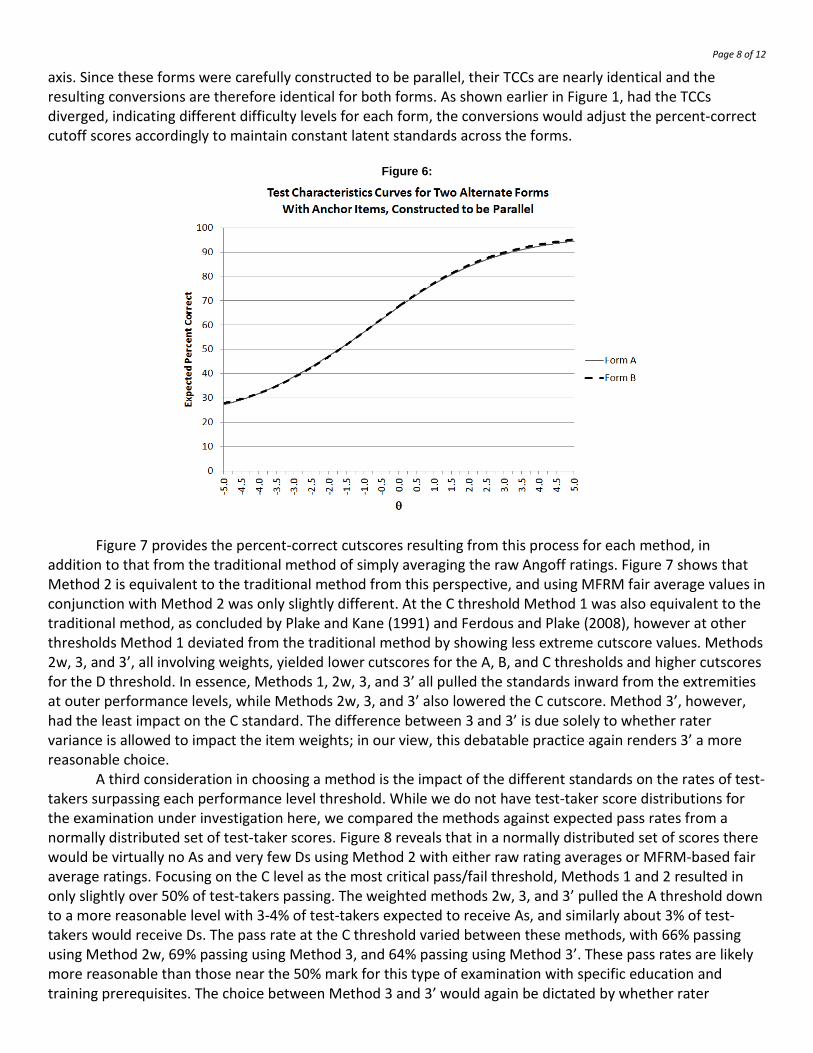
Looking at the results in Figure 5, it is apparent that Methods 1 and 2 were roughly equivalent only at the C threshold (comparable to the minimal competence threshold used in the Plake and Kane and Ferdous and Plake studies), while they diverged when ratings were made at other thresholds. Method 2 seemed unreasonably high at the A threshold in the current data, and applying the MFRM fair average values only exacerbated the divergence of Method 2 from other methods at thresholds other than C. The methods involving weights (2w, 3, and 3’) were not so extreme. Given the extremity of Method 2 in Figure 5 above, the conclusions of Hurtz et al. (2008) provide some comfort in choosing the standards derived through Method 3. However, since rater variance is allowed to influence the standards in Method 3 via their use in the weights, we favor Method 3’ which excludes this factor. A second consideration in deciding on the latent standard is to look at the impact of the different methods on percent-correct equivalents on the observed-score scale, as was the focus of Plake and Kane (1991) and Ferdous and Plake (2008). Figure 6 shows the TCCs for the two forms whose items were rated in this exam. Back-conversions from θ* to an observed cutscore for a given form involves locating the θ* along the horizontal axis of each form’s TCC and finding the corresponding expected percent-correct on the vertical

Page 8 of 12

axis. Since these forms were carefully constructed to be parallel, their TCCs are nearly identical and the resulting conversions are therefore identical for both forms. As shown earlier in Figure 1, had the TCCs diverged, indicating different difficulty levels for each form, the conversions would adjust the percent-correct cutoff scores accordingly to maintain constant latent standards across the forms.

Figure 6:

Figure 7 provides the percent-correct cutscores resulting from this process for each method, in addition to that from the traditional method of simply averaging the raw Angoff ratings. Figure 7 shows that Method 2 is equivalent to the traditional method from this perspective, and using MFRM fair average values in conjunction with Method 2 was only slightly different. At the C threshold Method 1 was also equivalent to the traditional method, as concluded by Plake and Kane (1991) and Ferdous and Plake (2008), however at other thresholds Method 1 deviated from the traditional method by showing less extreme cutscore values. Methods 2w, 3, and 3’, all involving weights, yielded lower cutscores for the A, B, and C thresholds and higher cutscores for the D threshold. In essence, Methods 1, 2w, 3, and 3’ all pulled the standards inward from the extremities at outer performance levels, while Methods 2w, 3, and 3’ also lowered the C cutscore. Method 3’, however, had the least impact on the C standard. The difference between 3 and 3’ is due solely to whether rater variance is allowed to impact the item weights; in our view, this debatable practice again renders 3’ a more reasonable choice.

A third consideration in choosing a method is the impact of the different standards on the rates of test-takers surpassing each performance level threshold. While we do not have test-taker score distributions for the examination under investigation here, we compared the methods against expected pass rates from a normally distributed set of test-taker scores. Figure 8 reveals that in a normally distributed set of scores there would be virtually no As and very few Ds using Method 2 with either raw rating averages or MFRM-based fair average ratings. Focusing on the C level as the most critical pass/fail threshold, Methods 1 and 2 resulted in only slightly over 50% of test-takers passing. The weighted methods 2w, 3, and 3’ pulled the A threshold down to a more reasonable level with 3-4% of test-takers expected to receive As, and similarly about 3% of test-takers would receive Ds. The pass rate at the C threshold varied between these methods, with 66% passing using Method 2w, 69% passing using Method 3, and 64% passing using Method 3’. These pass rates are likely more reasonable than those near the 50% mark for this type of examination with specific education and training prerequisites. The choice between Method 3 and 3’ would again be dictated by whether rater

Page 9 of 12

variance is considered an acceptable reason for the substantially different expected pass rates at the most critical C threshold. Our general perspective would give favor to the standards resulting from Method 3’.

Figure 7:

Figure 8:

To further explore the difference between Methods 3 and 3’, and whether excluding rater variance from the weights was a benefit or detriment to the process, we compared rater fit indices developed by van der Linden (1982) and Hurtz and Jones (2009). The error (E) index proposed by van der Linden, which is the

Page 10 of 12

average absolute deviation of the rating from the ICC at θ*, was .172 across performance levels for Method 3 and .167 for Method 3’; the corresponding values for the consistency (C) index were .769 and .778. Both E and C show a very slight improvement in fit when rater variance was excluded from the weights. Hurtz and Jones’ PWFI.10 index revealed that 46.9% of ratings fell within ±.10 of the ICCs for the Method 3 cutoff score, compared to a slightly larger 48.1% for Method 3’. Likewise, the PWFI.05 index showed 27.9% of ratings falling within ±.05 of the ICCs for Method 3 compared to the slightly larger 29.9% for Method 3’. These indices again show a small improvement in fit when differences in rater variances were removed from the weights. Helping to better understand the nature of the effects of using versus not using the rater variance in the weights, Hurtz and Jones’ rater balance (RB) index revealed that ratings tended to be biased upward (RB = .04) with respect to the ICCs at θ* when rater variances were used while they tended to be balanced above and below the ICCs (RB = .00) when rater variances were excluded from the weights when deriving θ*. The largest differences in RB were at the C and B thresholds where the respective values were .12 and .06 for Method 3, versus .03 and -.01 for Method 3’. Note that it was at these thresholds that the θ* values differed the most in Figure 5, leading to the greatest differences in percent-correct equivalents (Figure 6) and expected pass rates (Figure 7). The overall pattern of findings with respect to these rater fit indices suggests that using rater variances in the weights for Method 3 contributed to a greater misalignment of ratings with respect to the ICCs and negatively impacted the accuracy of the resulting θ*, lending further support to the θ* values from Method 3’ as the optimal choice. Using the Latent Standards to Define Performance Expectations

Once identified, the latent standards can be used to add details to the definitions of expected performance levels and to the construct map (Perie, 2008; Wyse, 2013). When explicating a construct map the continuum is conceptualized along two parallel dimensions as displayed in Figure 9: The arrangement of respondent abilities from high to low and the corresponding arrangement of item responses matched to different ability levels. In the context of the example to be used in the current paper, Figure 9 displays four thresholds of interest along the respondent ability continuum. Each can be explicated by identifying items that challenge test-takers at each threshold. This can be repeated for each major content domain within the test plan.

While a complete example with actual item content is not available for the test used in this paper due to test security concerns, the generic shell presented in Figure 9 displays an example of how the construct map would be used to define expectations of test-taker performance at each threshold. In this display, sample items with IRT b parameters falling at each threshold would be placed on the chart to operationally define the threshold in terms of actual test content. The table would be repeated for each content domain, with at least one item presented at each of the thresholds. These may be items that have been retired from active use due to overexposure but are still current and relevant, and because of the invariance property the specific exemplars can be swapped over time.

To help communicate expectations of test-taker performance via the construct map, they can be told the items are typical of those found to represent the competence levels of different test-takers. Starting from the bottom of the map and working upward, if they find an item fairly easy then they likely fall above that level of competence. As they move upward, if they find at a certain threshold that they are challenged to the point of feeling the likelihood of the correctness of their answer is about 50/50, they are near their competence level. By providing such a map, the expectations of different levels of performance are operationally defined in a meaningful way. Test-takers and educators/trainers can use the map to inform their training, and test-developers can use the map as guidance for item writing, using the exemplars as standards for comparison for writing new items at each targeted difficulty level. In future standard-setting efforts, perhaps focused on confirming the existing standards after the passage of a specified period of time or when

Page 11 of 12

changes to prerequisite training or test specifications have been made, the map can be used to guide future judgments of item difficulty.

Figure 9:

Construct Map Template for Defining Performance Expectations to Achieve Different Levels of Performance

Summary and Future Directions In this paper, as in similar recent work (Hurtz et al., 2012), we have argued that it is crucial in standard setting to distinguish the latent competence continuum from the observed score scale, and that focusing on the latent continuum provides the opportunity to derive invariant standards that can be applied across alternate forms constructed from a bank. We then compared several methods of deriving latent-scale standards from Angoff ratings, suggesting promising properties of a new method variant (called Method 3’ in this paper) that gives more weight to item ratings at each performance level for items providing their maximum information at that level. We then demonstrated how the latent-scale standards can be used as part of a construct map to operationally define the thresholds of each performance level in directly meaningful ways for presenting the information to stakeholders. Future research should continue to explore the relative merits of the different methods for deriving the latent-scale standards from Angoff ratings and methods for evaluating the invariance of the resulting standards across samples of both items and raters. In addition, future research should explore the utility and comprehensibility of the construct map format such as that depicted in Figure 9, or a much more elaborate form such as in Wyse (2013), from the perspectives of different stakeholders (test-takers, educators/trainers, test developers, standard-setters).

Page 12 of 12

References

Eckes, T. (2011). Introduction to many-facet Rasch measurement: Analyzing and evaluating rater-mediated assessments. New York: Peter Lang.

Engelhard, G. (1998). A binomial trials model for examining the ratings of standard-setting judges. Applied Measurement in Education, 11, 209-230.

Engelhard, G. (2013). Invariant measurement: Using Rasch models in the social, behavioral, and health sciences. New York: Routledge.

Ferdous, A. A., & Plake, B. S. (2008). Item response theory-based approaches for computing minimum passing scores from an Angoff-based standard-setting study. Educational and Psychological Measurement, 68, 779-796.

Hambleton, R. K., Swaminathan, H., & Rogers, H. J. (1991). Fundamentals of item response theory. Newbury Park, CA: Sage.

Hurtz, G. M., & Jones, J. P. (2009). Innovations in measuring rater accuracy in standard-setting: Assessing “fit” to item characteristic curves. Applied Measurement in Education, 22, 120-143.

Hurtz, G. M., Jones, J. P., & Jones, C. N. (2008). Conversion of proportion-correct standard-setting judgments to cutoff scores on the IRT θ scale. Applied Psychological Measurement, 32, 385-406.

Hurtz, G. M., Muh, V. P., Pierce, M. S., & Hertz, N. R. (2012, April). The Angoff method through the lens of latent trait theory: Theoretical and practical benefits of setting standards on the latent scale (where they belong). In Barney, M. (Chair). To raise or lower the bar: Innovations in standard setting. Symposium presented at the 27th Annual Conference of the Society for Industrial and Organizational Psychology, San Diego, CA.

Kaliski, P. K., Wind, S. A., Engelhard, G., Morgan, D. L., Plake, B. S., & Reshetar, R. A. (2013). Using the many-faceted Rasch model to evaluate standard setting judgments: An illustration with the advanced placement environmental science exam. Educational and Psychological Measurement, 73, 386-411.

Kane, M. T. (1987). On the use of IRT models with judgmental standard setting procedures. Journal of Educational Measurement, 24, 333-345.

Lewis D. M., Mitzel, H. C., & Green, D. R. (1996, June). Standard setting: A bookmark approach. In D. R. Green (Chair), IRT-Based Standard-Setting Procedures Utilizing Behavioral Anchoring. Symposium presented at the Council of Chief State School Officers National Conference on Large-Scale Assessment, Phoenix, AZ.

Lord, F. M., & Novick, M. R. (1968). Statistical theories of mental test scores. Reading, MA: Addison-Wesley.

Norcini, J. J. (1990). Equivalent pass/fail decisions. Journal of Educational Measurement, 27, 59–66.

Norcini, J. J., & Shea, J. A. (1992). Equivalent estimates of borderline group performance in standard setting. Journal of Educational Measurement, 29, 19–24.

Norcini, J. J., & Shea, J. A. (1997). The credibility and comparability of standards. Applied Measurement in Education, 10, 39–59.

Perie, M. (2008). A guide to understanding and developing performance-level descriptors. Educational Measurement: Issues and Practice, 27, 15-29.

Plake, B. S., & Kane, M. T. (1991). Comparison of methods for combining the minimum passing levels for individual items into a passing score for a test. Journal of Educational Measurement, 28, 249-256.

Stone, G. (2001). Objective standard setting (or truth in advertising). Journal of Applied Measurement, 1, 187-201.

van der Linden,W. J. (1982). A latent trait method for determining intrajudge inconsistency in the Angoff and Nedelsky techniques of standard-setting. Journal of Educational Measurement, 19, 295-308.

Wilson, M. (2005). Constructing measures: An item response modeling approach. Mahwah, NJ: Erlbaum.

Wyse, A. E. (2013). Construct maps as a foundation for standard setting. Measurement, 11, 139-170.