nchrp report 626 – ndt technology for quality assurance …€¦ · ndt technology for quality...
TRANSCRIPT

NDT Technology for Quality Assurance of
HMA Pavement Construction
NATIONALCOOPERATIVE HIGHWAYRESEARCH PROGRAMNCHRP
REPORT 626

TRANSPORTATION RESEARCH BOARD 2009 EXECUTIVE COMMITTEE*
OFFICERS
CHAIR: Debra L. Miller, Secretary, Kansas DOT, Topeka VICE CHAIR: Adib K. Kanafani, Cahill Professor of Civil Engineering, University of California, Berkeley EXECUTIVE DIRECTOR: Robert E. Skinner, Jr., Transportation Research Board
MEMBERS
J. Barry Barker, Executive Director, Transit Authority of River City, Louisville, KYAllen D. Biehler, Secretary, Pennsylvania DOT, HarrisburgJohn D. Bowe, President, Americas Region, APL Limited, Oakland, CALarry L. Brown, Sr., Executive Director, Mississippi DOT, JacksonDeborah H. Butler, Executive Vice President, Planning, and CIO, Norfolk Southern Corporation, Norfolk, VAWilliam A.V. Clark, Professor, Department of Geography, University of California, Los AngelesDavid S. Ekern, Commissioner, Virginia DOT, RichmondNicholas J. Garber, Henry L. Kinnier Professor, Department of Civil Engineering, University of Virginia, CharlottesvilleJeffrey W. Hamiel, Executive Director, Metropolitan Airports Commission, Minneapolis, MNEdward A. (Ned) Helme, President, Center for Clean Air Policy, Washington, DCWill Kempton, Director, California DOT, SacramentoSusan Martinovich, Director, Nevada DOT, Carson CityMichael D. Meyer, Professor, School of Civil and Environmental Engineering, Georgia Institute of Technology, AtlantaMichael R. Morris, Director of Transportation, North Central Texas Council of Governments, ArlingtonNeil J. Pedersen, Administrator, Maryland State Highway Administration, BaltimorePete K. Rahn, Director, Missouri DOT, Jefferson CitySandra Rosenbloom, Professor of Planning, University of Arizona, TucsonTracy L. Rosser, Vice President, Corporate Traffic, Wal-Mart Stores, Inc., Bentonville, ARRosa Clausell Rountree, Consultant, Tyrone, GAHenry G. (Gerry) Schwartz, Jr., Chairman (retired), Jacobs/Sverdrup Civil, Inc., St. Louis, MOC. Michael Walton, Ernest H. Cockrell Centennial Chair in Engineering, University of Texas, AustinLinda S. Watson, CEO, LYNX–Central Florida Regional Transportation Authority, OrlandoSteve Williams, Chairman and CEO, Maverick Transportation, Inc., Little Rock, AR
EX OFFICIO MEMBERS
Thad Allen (Adm., U.S. Coast Guard), Commandant, U.S. Coast Guard, Washington, DCRebecca M. Brewster, President and COO, American Transportation Research Institute, Smyrna, GAPaul R. Brubaker, Research and Innovative Technology Administrator, U.S.DOTGeorge Bugliarello, President Emeritus and University Professor, Polytechnic Institute of New York University, Brooklyn; Foreign Secretary,
National Academy of Engineering, Washington, DCSean T. Connaughton, Maritime Administrator, U.S.DOTClifford C. Eby, Acting Administrator, Federal Railroad Administration, U.S.DOTLeRoy Gishi, Chief, Division of Transportation, Bureau of Indian Affairs, U.S. Department of the Interior, Washington, DCEdward R. Hamberger, President and CEO, Association of American Railroads, Washington, DCJohn H. Hill, Federal Motor Carrier Safety Administrator, U.S.DOTJohn C. Horsley, Executive Director, American Association of State Highway and Transportation Officials, Washington, DCCarl T. Johnson, Pipeline and Hazardous Materials Safety Administrator, U.S.DOTDavid Kelly, Acting Administrator, National Highway Traffic Safety Administration, U.S.DOTSherry E. Little, Acting Administrator, Federal Transit Administration, U.S.DOTThomas J. Madison, Jr., Administrator, Federal Highway Administration, U.S.DOT William W. Millar, President, American Public Transportation Association, Washington, DCRobert A. Sturgell, Acting Administrator, Federal Aviation Administration, U.S.DOTRobert L. Van Antwerp (Lt. Gen., U.S. Army), Chief of Engineers and Commanding General, U.S. Army Corps of Engineers, Washington, DC
*Membership as of January 2009.

TRANSPORTAT ION RESEARCH BOARDWASHINGTON, D.C.
2009www.TRB.org
N A T I O N A L C O O P E R A T I V E H I G H W A Y R E S E A R C H P R O G R A M
NCHRP REPORT 626
Subject Areas
Materials and Construction
NDT Technology forQuality Assurance of
HMA Pavement Construction
Harold L. Von Quintus
Chetana RaoAPPLIED RESEARCH ASSOCIATES, INC.
Champaign, IL
Robert E. Minchin, Jr.UNIVERSITY OF FLORIDA
Gainesville, FL
Soheil NazarianUNIVERSITY OF TEXAS AT EL PASO
El Paso, TX
Kenneth R. MaserINFRASENSE, INC.
Arlington, MA
A N D
Brian ProwellNATIONAL CENTER FOR ASPHALT TECHNOLOGY
Auburn, AL
Research sponsored by the American Association of State Highway and Transportation Officials in cooperation with the Federal Highway Administration

NATIONAL COOPERATIVE HIGHWAYRESEARCH PROGRAM
Systematic, well-designed research provides the most effective
approach to the solution of many problems facing highway
administrators and engineers. Often, highway problems are of local
interest and can best be studied by highway departments individually
or in cooperation with their state universities and others. However, the
accelerating growth of highway transportation develops increasingly
complex problems of wide interest to highway authorities. These
problems are best studied through a coordinated program of
cooperative research.
In recognition of these needs, the highway administrators of the
American Association of State Highway and Transportation Officials
initiated in 1962 an objective national highway research program
employing modern scientific techniques. This program is supported on
a continuing basis by funds from participating member states of the
Association and it receives the full cooperation and support of the
Federal Highway Administration, United States Department of
Transportation.
The Transportation Research Board of the National Academies was
requested by the Association to administer the research program
because of the Board’s recognized objectivity and understanding of
modern research practices. The Board is uniquely suited for this
purpose as it maintains an extensive committee structure from which
authorities on any highway transportation subject may be drawn; it
possesses avenues of communications and cooperation with federal,
state and local governmental agencies, universities, and industry; its
relationship to the National Research Council is an insurance of
objectivity; it maintains a full-time research correlation staff of
specialists in highway transportation matters to bring the findings of
research directly to those who are in a position to use them.
The program is developed on the basis of research needs identified
by chief administrators of the highway and transportation departments
and by committees of AASHTO. Each year, specific areas of research
needs to be included in the program are proposed to the National
Research Council and the Board by the American Association of State
Highway and Transportation Officials. Research projects to fulfill these
needs are defined by the Board, and qualified research agencies are
selected from those that have submitted proposals. Administration and
surveillance of research contracts are the responsibilities of the National
Research Council and the Transportation Research Board.
The needs for highway research are many, and the National
Cooperative Highway Research Program can make significant
contributions to the solution of highway transportation problems of
mutual concern to many responsible groups. The program, however, is
intended to complement rather than to substitute for or duplicate other
highway research programs.
Published reports of the
NATIONAL COOPERATIVE HIGHWAY RESEARCH PROGRAM
are available from:
Transportation Research BoardBusiness Office500 Fifth Street, NWWashington, DC 20001
and can be ordered through the Internet at:
http://www.national-academies.org/trb/bookstore
Printed in the United States of America
NCHRP REPORT 626
Project 10-65ISSN 0077-5614ISBN: 978-0-309-11777-7Library of Congress Control Number 2009902460
© 2009 Transportation Research Board
COPYRIGHT PERMISSION
Authors herein are responsible for the authenticity of their materials and for obtainingwritten permissions from publishers or persons who own the copyright to any previouslypublished or copyrighted material used herein.
Cooperative Research Programs (CRP) grants permission to reproduce material in thispublication for classroom and not-for-profit purposes. Permission is given with theunderstanding that none of the material will be used to imply TRB, AASHTO, FAA, FHWA,FMCSA, FTA, or Transit Development Corporation endorsement of a particular product,method, or practice. It is expected that those reproducing the material in this document foreducational and not-for-profit uses will give appropriate acknowledgment of the source ofany reprinted or reproduced material. For other uses of the material, request permissionfrom CRP.
NOTICE
The project that is the subject of this report was a part of the National Cooperative HighwayResearch Program conducted by the Transportation Research Board with the approval ofthe Governing Board of the National Research Council. Such approval reflects theGoverning Board’s judgment that the program concerned is of national importance andappropriate with respect to both the purposes and resources of the National ResearchCouncil.
The members of the technical committee selected to monitor this project and to review thisreport were chosen for recognized scholarly competence and with due consideration for thebalance of disciplines appropriate to the project. The opinions and conclusions expressedor implied are those of the research agency that performed the research, and, while they havebeen accepted as appropriate by the technical committee, they are not necessarily those ofthe Transportation Research Board, the National Research Council, the AmericanAssociation of State Highway and Transportation Officials, or the Federal HighwayAdministration, U.S. Department of Transportation.
Each report is reviewed and accepted for publication by the technical committee accordingto procedures established and monitored by the Transportation Research Board ExecutiveCommittee and the Governing Board of the National Research Council.
The Transportation Research Board of the National Academies, the National ResearchCouncil, the Federal Highway Administration, the American Association of State Highwayand Transportation Officials, and the individual states participating in the NationalCooperative Highway Research Program do not endorse products or manufacturers. Tradeor manufacturers’ names appear herein solely because they are considered essential to theobject of this report.


CRP STAFF FOR NCHRP REPORT 626
Christopher W. Jenks, Director, Cooperative Research ProgramsCrawford F. Jencks, Deputy Director, Cooperative Research ProgramsEdward T. Harrigan, Senior Program OfficerEileen P. Delaney, Director of PublicationsKami Cabral, Editor
NCHRP PROJECT 10-65 PANELField of Materials and Construction—Area of Specifications, Procedures, and Practices
Jimmy W. Brumfield, Burns Cooley Dennis, Inc., Jackson, MS (Chair)Terrie Bressette, California DOT, Sacramento, CA Bouzid Choubane, Florida DOT, Gainesville, FL Gregory S. Cleveland, HDR, Inc., Pflugerville, TX Ronald Cominsky, Pennsylvania Asphalt Pavement Association, Harrisburg, PA Roger L. Green, Ohio DOT, Columbus, OH Larry L. Michael, Hagerstown, MD Stefan A. Romanoschi, University of Texas - Arlington, Arlington, TX Kim A. Willoughby, Washington State DOT, Olympia, WA Katherine A. Petros, FHWA Liaison Victor “Lee” Gallivan, Other Liaison David E. Newcomb, Other Liaison Frederick Hejl, TRB Liaison
C O O P E R A T I V E R E S E A R C H P R O G R A M S
This report contains the findings of research performed to investigate the applicationof nondestructive testing (NDT) technologies in the quality assurance of hot mix asphalt(HMA) pavement construction. The report contains the results and analyses of the researchperformed and presents several key products, notably a recommended manual of practicewith guidelines for implementing selected NDT technologies in an agency’s routine qualityassurance (QA) program for HMA pavement construction and detailed test methods for therecommended NDT technologies. Thus, the report will be of immediate interest to con-struction and materials engineers in state highway agencies and the private sector.
Test methods used for in-place quality assurance of individual HMA and unbound pave-ment layers have changed little in past decades. Such quality assurance programs typicallyrely on nuclear density measurements or the results of testing conducted on pavementcores. Roughness measurements are often used to confirm that the newly constructed pave-ment has an adequate initial smoothness.
More recently, NDT methods, including lasers, ground-penetrating radar, falling weightdeflectometers, penetrometers, and infrared and seismic technologies, have been signifi-cantly improved and have shown potential for use in the quality assurance of HMA pave-ment construction. Furthermore, the new Mechanistic-Empirical Pavement Design Guide(MEPDG) uses pavement layer stiffness modulus as a key material property for design ofnew and rehabilitated HMA pavements. The availability of this tool to predict pavementperformance will lead to increased measurement of layer moduli by owner agencies, anactivity that has not been a typical component in the past for HMA project acceptance.
This research had two objectives. The first was to conduct a comprehensive field experi-ment to determine the effectiveness and practicality of promising, existing NDT technolo-gies for the evaluation of the quality of unbound and bound pavement layers during orimmediately after placement or for acceptance of the entire HMA pavement at its comple-tion. The second objective was to prepare a recommended manual of practice and test meth-ods for those NDT technologies judged ready for implementation by AASHTO.
The research identified several NDT technologies with the potential for immediate imple-mentation in a quality assurance program of HMA pavement construction, including thatof individual HMA, base, and subgrade layers. This was assessed based on (1) the ability toaccurately identify construction anomalies and (2) the ability to predict material propertiesindicative of pavement performance. The GeoGauge is the device recommended for esti-mating the modulus of unbound layers, while the portable seismic pavement analyzer(PSPA) is recommended for estimating the modulus of HMA layers. The PaveTracker is alsorecommended for use in establishing and confirming the rolling pattern for HMA layers.
F O R E W O R D
By Edward T. HarriganStaff OfficerTransportation Research Board
These recommendations do not mean that other NDT devices included in the evaluation—e.g., the dynamic cone penetrometer (DCP), ground penetrating radar (GPR), the electri-cal density gauge (EDG), and the pavement quality indicator (PQI)—do not provide use-ful data for pavement and materials testing purposes. Several of these devices demonstrateddistinct benefits and advantages that are documented in this report for routine pavementevaluation, but were judged to require additional development or evaluation before they arefully implemented in routine practice for QA of HMA pavements.
The research was performed by Applied Research Associates, Inc. The report fully docu-ments the research leading to the recommended manual of practice and NDT methods. Therecommendations are under consideration for possible adoption by the AASHTO HighwaySubcommittee on Construction and Subcommittee on Materials.

C O N T E N T S
1 Summary1 Introduction2 NDT Devices Included in the Field Evaluation7 Projects and Materials Included in the Field Evaluation8 Field Evaluation of NDT Devices
18 Conclusions21 Recommendations
23 Data Interpretation and Application
24 Chapter 1 Applicability of NDT Technologies on Construction Projects
24 1.1 Ultrasonic—PSPA and DSPA 26 1.2 Steady-State Vibratory—GeoGauge27 1.3 Deflection-Based Methods30 1.4 Dynamic Cone Penetrometer31 1.5 Ground Penetrating Radar33 1.6 Electric Current/Electronic Methods35 1.7 Intelligent Compactors/Rollers with Mounted Response Measuring Devices36 1.8 Summary of Process Impact
38 Chapter 2 Materials Testing for Construction Quality Determination
38 2.1 Identification of Material Anomalies and Differences42 2.2 Estimating Target Modulus Values51 2.3 Accuracy and Precision57 2.4 Comparison of Results Between NDT Technologies67 2.5 Supplemental Comparisons74 2.6 Summary of Evaluations
80 Chapter 3 Construction Quality Determination80 3.1 Quality Control and Acceptance Application80 3.2 Control Limits for Statistical Control Charts81 3.3 Parameters for Determining PWL
84 References
85 Appendix A Glossary
87 Appendix B Volume 1—Procedural Manual

AUTHOR ACKNOWLEDGMENTS
The research described herein was performed under NCHRP Project 10-65 by the Transportation Sec-tor of Applied Research Associates (ARA), Inc. Mr. Harold L. Von Quintus served as the Principal Inves-tigator on the project.
Mr. Von Quintus was assisted by Dr. Chetana Rao of ARA as the Project Manager and Engineer on theteam. The team also included Richard Stubstad of ARA; Dr. Kenneth Maser with Infrasense; Dr. SoheilNazarian, with the University of Texas at El Paso (UTEP); Mr. Brian Prowell with the National Center forAsphalt Technology (NCAT); and Dr. Edward Minchin with the University of Florida, Gainesville.
In addition, the project team was supported by several individuals who conducted field testing, includ-ing Mr. Ajay S. Singh, Mr. Brandon Artis, and Mr. David Goodin from ARA; Mr. Manuel Celaya fromUTEP; and Mr. Dennis Andersen from EDG, LLC. Dr. Brian Prowell from NCAT and Dr. Allen Cooleyfrom BCD, Inc., provided oversight for laboratory testing of asphalt and unbound materials, respectively.Dr. Buzz Powell assisted with coordinating field tests at the NCAT test track during the construction ofthe test tracks. Mr. Brandon Von Quintus, Mr. Ajay Singh, and Mr. Mark Stanley of ARA assisted withdevelopment of databases for field test results and in preparation of field notes from test sites. Ms. RobinJones, Ms. Jaime DeCaro, and Ms. Alicia Pitlik provided editorial review, final report formatting, and tab-ulation of appendices, respectively.
The project team also appreciates and acknowledges the support and technical assistance of variousagency and contractor personnel, as well as representatives from nondestructive testing equipment man-ufacturers who were involved in the construction and testing of pavement structures and mixturesincluded in various phases of the project. Those individuals directly involved in the coordination and con-struction of the projects included in the field testing plan are listed as follows:
Minnesota: Mr. John Siekmier (Minnesota DOT), Mr. Art Bolland (Minnesota DOT), Mr. Chris Dun-nick (Dunnick Brothers)
Alabama: Ms. Sharon Fuller (Alabama DOT), Mr. Andy Carol (Scott Bridge Company), East AlabamaPaving
Texas: Mr. Tom Scullion (Texas Transportation Institute), Mr. Gregory Cleveland (Texas DOT), Mr. James Klotz (Texas DOT), Mr. Tim Wade (Texas Turnpike Authority), Dr. Weng-On Tam (AvlisEngineering), Texas Lone Star Infrastructure
Missouri: Mr. John Donahue (Missouri DOT), Mr. Tim Hellebusch (Missouri DOT)North Dakota: Mr. Bryon Fuchs (North Dakota DOT), Mr. Joel Wilt (North Dakota DOT), Mr. Greg
Semenko (North Dakota DOT)Ohio: Mr. Roger Green (Ohio DOT), Mr. Brian French (Ohio DOT)NDT Devices and IC Rollers: Mr. Chris Connelly (BOMAG), Mr. Jeff Fox (Ammann), Mr. Christopher
Dumas (FHWA), Mr. Bob Horan (Salut), Mr. Scott Fielder (Humbolt Scientific, Inc. [Part A testing]),Mr. Melvin Main (Humboldt Scientific, Inc. [Part B testing]), Mr. William Beck, (Dynatest), Caterpillar,Fugro/CarlBro, Transtech Systems Inc., Troxler Electronic Laboratories, Inc.

S U M M A R Y
Introduction
Quality assurance (QA) programs provide the owner and contractor a means to ensure that thedesired results are obtained to produce high-quality, long-life pavements. Desired results are thosethat meet or exceed the specifications and design requirements. Traditional pavement constructionquality control and quality acceptance (QC/QA) procedures include a variety of laboratory andfield test methods that measure volumetric and surface properties of pavement materials. Thetest methods to measure the volumetric properties have changed little within the past couple ofdecades.
More recently, nondestructive testing (NDT) methods, including lasers, ground-penetratingradar (GPR), falling weight deflectometers (FWD), penetrometers, and infrared and seismictechnologies have been improved significantly and have shown potential for use in the QC/QA offlexible pavement construction. Furthermore, the new Mechanistic-Empirical Pavement DesignGuide (MEPDG) uses layer modulus as a key material property. This should lead to increasedmeasurement of layer moduli—a material property that can be estimated through NDT tests,which is not included, at present, in the acceptance plan.
This research study investigated the application of existing NDT technologies for measuringthe quality of flexible pavements. Promising NDT technologies were assessed on actual fieldprojects for their ability to evaluate the quality of pavement layers during or immediately afterplacement or to accept the entire pavement at its completion. The results from this projectidentified NDT technologies ready and appropriate for implementation in routine, practicalQC/QA operations.
Objectives
The overall objective of NCHRP Project 10-65 was to identify NDT technologies that haveimmediate application for routine, practical QA operations to assist agency and contractorpersonnel in judging the quality of hot mix asphalt (HMA) overlays and flexible pavementconstruction. This objective was divided into two parts:
1. Conduct a field evaluation of selected NDT technologies to determine their effectiveness andpracticality for QC/QA of flexible pavement construction.
2. Recommend appropriate test protocols based on the field evaluation and test results.
Effectiveness and practicality are key words in the first part of the objective. The field evaluation plan was developed to determine the effectiveness and practicality of different
NDT Technology for Quality Assurance of HMA Pavement Construction
1

2
NDT technologies for use in QA programs. These terms are defined as follows for NCHRPProject 10-65:
• Effectiveness of NDT Technology—Ability or capability of the technology and device todetect changes in unbound materials or HMA mixtures that affect the performance anddesign life of flexible pavements and HMA overlays.
• Practicality of NDT Technology—Capability of the technology and device to collect andinterpret data on a real-time basis to assist project construction personnel (QC/QA) inmaking accurate decisions in controlling and accepting the final product.
Integration of Structural Design, Mixture Design, and Quality Assurance
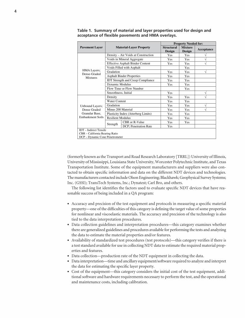
The approach taken for this project was to use fundamental properties that are needed forboth mixture and structural design for both control and acceptance of flexible pavements andHMA overlays. Figure 1 illustrates this integration or systems approach. The material or layerproperties were grouped into three areas—volumetric, structural, and functional—and the NDTtechnologies were evaluated for their ability to estimate these properties accurately. Using thesame mixture properties for accepting the pavement layer that were used for structural and mix-ture design allows the agency to more precisely estimate the impact that deficient materials andpavement layers have on performance. The material tests that are needed for structural andmixture design using the newer procedures are listed in Table 1.
Two structural properties that are needed to predict the performance of flexible pavementsand HMA overlays are modulus and thickness. These are called “quality characteristics,” andthey are defined in Transportation Research Circular E-C037 as “That characteristic of a unitor product that is actually measured to determine conformance with a given requirement.When the quality characteristic is measured for acceptance purposes, it is an acceptance qualitycharacteristic (AQC).”
Products
The final deliverables for NCHRP Project 10-65 were divided into three volumes. Volume 1is the procedural manual for implementing the NDT methods for QA application. It is includedherein as Appendix B. It contains some of the examples for application of the modulus valuesfor controlling and accepting flexible pavements. Volume 2 is the standard NCHRP final report.Part 3 of Volume 2 is the main body of NCHRP Report 626. Volume 3 includes the appendicesfor the other two volumes. It is not published herein. The appendices in Volume 3 also include thedata generated from this project. The complete three volumes are presented in NCHRP Web-OnlyDocument 133.
NDT Devices Included in the Field Evaluation
A large number of NDT technologies and devices have been used for pavement evaluation andforensic studies. Table 2 summarizes the technologies and methods that have been used to mea-sure different properties and features of flexible pavements. As tabulated, GPR has been used forestimating many more volumetric properties and features than any other NDT technology, whilethe deflection and ultrasonic-based technologies have been used more for estimating structuralproperties and features.
To narrow the list of NDT devices that have potential for QA application, several highwayagencies were contacted to collect information on their practices and experiences. Research

reports of several agencies were also reviewed. These agencies include Arizona, California,Connecticut, Florida, Georgia, Illinois, Maryland, New Hampshire, Minnesota, Mississippi,Missouri, Nevada, Ohio, Oklahoma, Pennsylvania, Texas, Virginia, Washington, and WisconsinDepartments of Transportation (DOTs), the Federal Aviation Administration (FAA), FederalHighway Administration (FHWA), Eastern Federal Lands Division, Central Federal LandsDivision, U.S. Air Force, U.S. Army Corps of Engineers Engineer Research and DevelopmentCenter, Loughborogh University, Nottingham Trent University, Transport Research Laboratory
3
Select Strategy: Trial cross-sections for
pavement structural design or rehabilitation.
Complete structural design using mixture specifications; Select structural properties to minimize distress.
Material selection & certification; Source
approval.
MaterialSpecifications:
Aggregate, Asphalt Binder, Additives, etc.
Volumetric Mixture Design; Superpave
Gyratory Compactor
Feedback from
monitoringpavement
performance, NCHRP
Project 9-30
Confirmation – Adjustment of
volumetricmixture design.
Prepare specimens over range of
volumetric conditions.Perform NDT QA tests
on laboratory test specimens.
Mix Design Tests, NCHRP Project 9-33
QA Tests; NCHRP Project
10-65
Select final mixture design & measure E* master curve.
Field Verification of Mixture Design
Select/Establish QA criteria for measuring quality;
determine seismic design modulus.
Agency Acceptance Plan & Specifications
Contractor Quality Control Plan
Pavement Management: Monitoring projects – Functional, Structural,
Volumetric Properties & Surface Distress.
Confirmationof structural
designassumptions & performanceexpectations
Perform torture test(s) (APA, Hamburg, etc.) or Dynamic modulus, fracture, permanent deformation tests,
etc.; NCHRP Project 9-19.
Site Features & Inputs:Climate TrafficFoundation
Structural Design, NCHRP Project 1-
37A
Calibrate NDT QA tests; control strips, NCHRP
Project 10-65.
PRS, NCHRP
Project 9-22
Figure 1. Example flow chart for the systems approach for specifying, designing, and placing quality HMA mixtures.
4
(formerly known as the Transport and Road Research Laboratory [TRRL]) University of Illinois,University of Mississippi, Louisiana State University, Worcester Polytechnic Institute, and TexasTransportation Institute. Some of the equipment manufacturers and suppliers were also con-tacted to obtain specific information and data on the different NDT devices and technologies.The manufacturers contacted include Olson Engineering; Blackhawk; Geophysical Survey Systems;Inc. (GSSI); TransTech Systems, Inc.; Dynatest; Carl Bro, and others.
The following list identifies the factors used to evaluate specific NDT devices that have rea-sonable success of being included in a QA program:
• Accuracy and precision of the test equipment and protocols in measuring a specific materialproperty—one of the difficulties of this category is defining the target value of some propertiesfor nonlinear and viscoelastic materials. The accuracy and precision of the technology is alsotied to the data interpretation procedures.
• Data collection guidelines and interpretation procedures—this category examines whetherthere are generalized guidelines and procedures available for performing the tests and analyzingthe data to estimate the material properties and/or features.
• Availability of standardized test procedures (test protocols)—this category verifies if there isa test standard available for use in collecting NDT data to estimate the required material prop-erties and features.
• Data collection—production rate of the NDT equipment in collecting the data.• Data interpretation—time and ancillary equipment/software required to analyze and interpret
the data for estimating the specific layer property.• Cost of the equipment—this category considers the initial cost of the test equipment, addi-
tional software and hardware requirements necessary to perform the test, and the operationaland maintenance costs, including calibration.
Property Needed for: Pavement Layer Material-Layer Property Structural
DesignMixtureDesign
Acceptance
Density – Air Voids at Construction Yes Yes Voids in Mineral Aggregate Yes Yes Effective Asphalt Binder Content Yes Yes Voids Filled with Asphalt Yes Gradation Yes Yes Asphalt Binder Properties Yes Yes IDT Strength and Creep Compliance Yes Yes Dynamic Modulus Yes Yes Flow Time or Flow Number Yes
HMA Layers; Dense-Graded
Mixtures
Smoothness, Initial YesDensity Yes Yes Water Content Yes Yes Gradation Yes Yes Minus 200 Material Yes Yes Plasticity Index (Atterberg Limits) Yes Yes Resilient Modulus Yes Yes
CBR or R-Value Yes Yes
Unbound Layers; Dense Graded Granular Base,
Embankment Soils
StrengthDCP; Penetration Rate Yes
IDT – Indirect Tensile CBR – California Bearing Ratio DCP – Dynamic Cone Penetrometer
Table 1. Summary of material and layer properties used for design andacceptance of flexible pavements and HMA overlays.

5
• Complexity of the equipment or personnel training requirements.• Ability of the test method and procedure to quantify the material properties needed for QA,
mixture design, and structural design (see Figure 1). In other words, is the NDT test resultapplicable to mixture and structural design?
• Relationship between the test result and other traditional and advanced tests used in mixturedesign and structural design.
NDT Technologies and MethodsType of Property or Feature
HMA Layers Unbound Aggregate Baseand Soil Layers
Density GPRNon-Nuclear Gauges; PQI, PaveTracker
GPRNon-Nuclear Gauges; EDG, Purdue TDR
Air Voids or Percent
Compaction
GPRInfrared Tomography Acoustic Emissions Roller-Mounted Density Devices
GPRRoller-Mounted Density Devices
Fluids Content GPRGPRNon-Nuclear Gauges; EDG, Purdue TDR
Gradation;Segregation
GPRInfrared Tomography ROSAN
NA
Volumetric
Voids in Mineral Aggregate GPR (Proprietary Method) NA
Thickness
GPRUltrasonic; Impact Echo, SPA, SASW Magnetic Tomography
GPRUltrasonic; SASW, SPA
Modulus; Dynamic or Resilient
Ultrasonic; PSPA, SASW Deflection-Based; FWD, LWD, Roller-Mounted Response Systems; Asphalt Manager
Impact/Penetration; DCP, Clegg Hammer Ultrasonic; DSPA, SPA, SASW Deflection-Based; FWD, LWD Steady-State Vibratory; GeoGaugeRoller-Mounted Response Systems
Structural
Bond/Adhesion Between Lifts
Ultrasonic; SASW, Impulse Response Infrared Tomography
NA
Profile; IRI Profilograph, Profilometer, Inertial Profilers
NA
Noise Noise Trailers NAFunctional
Friction CT Meter, ROSAN NASPA – Seismic Pavement Analyzer PSPA – Portable Seismic Pavement Analyzer SASW – Spectral Analysis of Surface Waves LWD – Light Weight Deflectometer ROSAN - ROad Surface ANalyzer EDG – Electrical Density Gauge TDR – Time Domain Reflectometry DSPA – Dirt Seismic Pavement Analyzer PQI – Pavement Quality Indicator DCP – Dynamic Cone Penetrometer CT – Circular Texture FWD – Falling Weight Deflectometer
Table 2. NDT methods used to measure properties and features of flexiblepavements in place.

6
NDT Devices Included in the Field Evaluation
The following list contains, in no particular order, the NDT technologies and devices that wereselected for use in the field study:
• Deflection Based Technologies—The FWD and LWD were selected because of the largenumber of devices that are being used in the United States and the large database that has beencreated under the FHWA Long Term Pavement Performance (LTPP) program. The LWDwas used to evaluate individual layers, especially unbound layers, while the FWD was used toevaluate the entire pavement structure at completion to ensure that the flexible pavementstructure or HMA overlay met the overall strength requirements used in the structural designprocess. Deflection measuring devices are readily available within most agencies for immedi-ate use in QA.
• Dynamic Cone Penetrometer—The DCP was selected because of its current use in QA oper-ations in selected agencies and its ability to estimate the in-place strength of unbound layersand materials. In addition, the DCP does not require extensive support software for evaluatingthe test results. DCP equipment is being manufactured and marketed by various organizations,making it readily available.
• Ground Penetrating Radar—GPR was selected because of its current use in pavement foren-sic and evaluation studies for rehabilitation design and for estimating both the thickness andair voids of pavement layers. If proven successful, this will be one of the more importantdevices used for acceptance of the final product by agencies, assuming that the interpretationof the data can become more readily available on a commercial basis. The GPR air-coupledantenna was used successfully within the FHWA-LTPP program to measure the layer thicknesswithin many of the 500-ft test sections.
• Seismic Pavement Analyzer—Both the PSPA and DSPA were selected because they providea measure of the layer modulus and can be used to test both thin and thick layers during andshortly after placement. This technology can also be used in the laboratory to test both HMAand unbound materials compacted to various conditions (e.g., different water contents forunbound materials and soils or temperature and asphalt content for HMA to evaluate the effectof fluids and temperature).
• GeoGauge—The GeoGauge has had mixed results in testing unbound pavement layers in thepast. It was selected for this study because it is simple to use and provides a measure of theresilient modulus of unbound pavement layers and embankment soils and can be used to testtypical lift thicknesses.
• Non-Nuclear Electric Gauges; Non-Roller-Mounted Devices—Non-nuclear density gaugeshave a definite advantage over the nuclear devices simply from a safety standpoint. Thesegauges have been used on many projects but with varying results. They were selected for thecurrent study because the devices have been significantly improved since their previous eval-uations. Moreover, many agencies are allowing their use by contractors for QC, and someagencies are beginning to use the contractor QC results for acceptance. They also representthe baseline comparison to the results from the nuclear gauges for measuring density for usein acceptance procedures. Thus, non-nuclear density gauges that provide location-specificresults were selected for evaluation under this study. The gauges selected for initial use were thePQI and PaveTracker for HMA mixtures, while the EDG was selected for unbound materials.
NDT Devices Excluded from the Field Evaluation
The following list contains NDT technologies and devices that were excluded from the fieldevaluation study. It also contains explanations for the exclusion.

7
• Roller-Mounted-Density/Stiffness Devices—Non-nuclear density and stiffness monitoringdevices attached to the rollers (for example, the BOMAG Varicontrol and Onboard Measur-ing System) were excluded because these devices have not been extensively used for QC, fewagencies are evaluating this technology for possible use in the future, and there are a limitednumber of these rollers available for contractor use. Although the roller-mounted devices wereexcluded from the field evaluation, the roller manufacturers were contacted to determine theiravailability for use on selected projects.
• Surface Condition Systems—None of the surface condition measuring systems or deviceswas suggested for further evaluation under NCHRP Project 10-65. Although the initial Interna-tional Roughness Index (IRI) is an input to the MEPDG, the smoothness measuring devicesused for acceptance of the wearing surface are already included in the QA programs of manyagencies. In addition, none of the devices provides an estimate of the volumetric and struc-tural properties of the wearing surface.
• Noise and Friction Methods—Noise and friction measuring devices were excluded from furtherconsideration because these properties are not needed in the MEPDG or any other structuraldesign procedure, and no agency is considering their use for acceptance.
• Infrared Tomography—Infrared cameras and sensors were excluded from the field evaluationbecause their output only provides supplemental information to current acceptance plans. Inother words, the devices are used to identify “cold spots” or temperature anomalies. Other testmethods are still used to determine whether the contractor has met the density specification.This statement does not imply that this technology should be abandoned or not used—theinfrared cameras and sensors do provide good information and data on the consistency ofthe HMA being placed by the contractor. However, they do not provide information that isrequired for QA programs.
• Other Ultrasonic Test Methods—Impact echo and impulse response methods, as well asthe ultrasonic scanners, were excluded because they are perceived to have a high risk of implementation into practical and effective QA operations.
• Continuous Deflection-Based Devices—Rolling wheel deflectometers that are under devel-opment were also excluded from the field evaluation. These devices are considered to be inthe research and development stage and are not ready for immediate application into a QAprogram.
Projects and Materials Included in the Field Evaluation
The field evaluation was divided into two parts, referred to as Parts A and B. The primarypurpose of the Part A field evaluation was to accept or reject the null hypothesis that a givenNDT technology or device can accurately identify construction anomalies or physical differ-ences along a project. A secondary purpose of this part of the field evaluation was to confirmthat the NDT device can be readily and effectively implemented into routine QA programs forflexible pavement construction and HMA overlays—an impact assessment. Part B of the fieldevaluation was to use those NDT technologies and devices selected from Part A and refine thetest protocols and data interpretation procedures for judging the quality of flexible pavementconstruction. Part B also included identifying limitations and boundary conditions of selectedNDT test methods.
Table 3 lists the projects and materials included in the field evaluation, while Table 4 lists thosedefects and layer differences that should have an impact on the quality characteristics measuredby the QA tests. Table 5 contains the anomalies and differences of unbound material sectionsplaced along each project. Likewise, Table 6 lists the anomalies and differences of HMA layers.None of the NDT operators were advised of these anomalies or physical differences.

8
Field Evaluation of NDT Devices
Identifying Anomalies and Physical Differences
A standard t-test and the Student-Newman-Keuls (SNK) mean separation procedure using a95 percent confidence level were used to determine whether the areas with anomalies or physicaldifferences were significantly different from the other areas tested. Table 7 lists identificationof the physical differences of the unbound and HMA layers within a project. The DSPA andGeoGauge are considered acceptable in identifying localized differences in the physical conditionof unbound materials, while the PSPA and PQI were considered acceptable for the HMA layers.
Part Project Identification & Location Layer/Material EvaluatedHMA Dense-Graded Base Mixture
Granular Base Class 6, Crushed Aggregate A 1
TH-23 Reconstruction Project; Wilmar/Spicer Minnesota Class 5
EmbankmentLow Plasticity, Improved Soil with Gravel & Large Aggregate Particles
A 2 I-85 Overlay Project; Auburn, Alabama
HMA12.5 mm Stone Matrix Asphalt Mix; PG76-22
HMA Coarse-Graded Base Mixture; PG67-22 Granular Base Crushed Limestone Base A 3
US-280 Reconstruction Project; Opelika, Alabama
Embankment Improved Soil; Aggregate-Soil Mix
A 4 I-85 Ramp Construction Project; Auburn, Alabama
Embankment Low Plasticity, Fine-Grained Soil
HMACoarse-Graded 19 mm Base Mixture; PG64-22
A 5 SH-130 New Construction Project; Georgetown, Texas
EmbankmentCoarse-Grained Aggregate/Soil; Improved Soil
A 6 SH-21 Widening Project; Caldwell, Texas
SubgradeHigh Plasticity Fine-Grained Soil with Gravel
HMA Coarse-Graded Base Mixture B 7
US-47 Widening Project; St. Clair, Missouri HMA Fine-Graded Wearing Surface
B 8 I-75 Rehabilitation Project, Rubblization; Saginaw, Michigan
HMA Dense-Graded Binder Mixture; Type 3C
HMA Coarse-Graded Base Mix; PG58-28
Granular Base Crushed Gravel with Surface Treatment; Class 5 B 9 US-2 New Construction; North Dakota
Embankment Soil-Aggregate Mixture HMA Coarse-Graded Binder Mixture
B 10 US-53 New Construction; Toledo, Ohio Granular Base Crushed Aggregate; Type 304
B 11 I-20 Overlay; Odessa, Texas HMA Coarse-Graded Mixture; CMHB B 12 County Road 103; Pecos, Texas Granular Base Caliche, Aggregate Base
NCAT; Alabama Overlay, Section E-5, Opelika, Alabama
HMAWearing Surface with 45% RAP; PG67, no modifiers used.
NCAT; Alabama Overlay, Section E-6, Opelika, Alabama
HMAWearing Surface with 45% RAP; PG76 with SBS. B 13
NCAT; Alabama Overlay, Section E-7, Opelika, Alabama
HMAWearing Surface with 45% RAP; PG76 with Sasobit.
HMA PMA Mixture with SBS; PG76 HMA Neat Asphalt Binder Mix; PG67 B 14
NCAT; Florida; Structural Test Sections N-1 & N-2
Granular Base Limerock Base HMA Polymer Modified Asphalt Mix; PG76 (SBS) HMA Neat Asphalt Binder Mix; PG64 B 15
NCAT; Missouri; Structural Test Section N-10
Granular Base Crushed Limestone
B 16 NCAT; Oklahoma; Structural Test Sections N-8 & N-9
Subgrade Soil High Plasticity Clay with Chert Aggregate
HMA Coarse-Graded Base Mix; PG67; Limestone B 17
NCAT; Alabama; Structural Test Section S-11 Granular Base Crushed Granite Base
CMHB – Coarse Matrix, High Binder Content (mixture type term used by the Texas DOT specifications) PG – Performance Grade PMA – Polymer Modified Asphalt RAP – Recycled Asphalt Pavement
Table 3. Projects and material types included in the field evaluation.

9
Estimating Laboratory Measured Moduli
Laboratory measured modulus of a material is an input parameter for all layers in mechanistic-empirical (M-E) pavement structural design procedures, including the MEPDG. Resilient mod-ulus is the input for unbound layers and soils, while the dynamic modulus is used for all HMAlayers. The values determined by each NDT modulus estimating device (DCP, DSPA, PSPA,GeoGauge, and deflection-based devices) were compared to the moduli measured in the labo-ratory on test specimens compacted to the density of the in-place layer. Different stress stateswere used for determining the resilient modulus of unbound layers, while different frequencies atthe in-place mat temperature were used to determine the dynamic modulus of the HMA layers.
None of the NDT devices accurately predicted the modulus values that were measured in thelaboratory for the unbound materials and HMA mixtures. However, all of the modulus estimat-ing NDT devices did show a trend of increasing moduli with increasing laboratory measuredmoduli.
Unbound Materials and Layers; Embankments
All projects
No construction defect was observed in any of the Parts A and B projects. As listed in Table 5, however, there were differences in the condition of the base materials and embankments that were planned to ensure that the NDT devices would identify those differences.
HMA Mixtures
US-280 HMA Base
Truck-to-truck segregation observed in some areas. Cores were taken in these areas, but some of the cores disintegrated during the wet coring process.
In addition, a significant difference in dynamic modulus was found between the initial and supplemental sections included in the test program. The supplemental section was found to have much higher dynamic modulus values. This difference was not planned.
I-85 SMA Overlay No defects noted. TH-23 HMA Base No defects noted.
SH-130 HMA Base
No defects noted during the time of testing, but there was controversy on the mixture because it had been exhibiting checking during the compaction process. Changes were made to the mixture during production. The change made and the time that the change was made were unclear relative to the time of the NDT evaluation.
US-47 HMA Base The mixture was tender; and shoved under the rollers.
US-47 Wearing Surface Portions of this mixture were rejected by the agency in other areas of the project.
I-75 HMA Base, Type 3-C No defects noted, but mixture placed along the shoulder was tender.
I-75 HMA, Type E3 & E10 No defects noted, but portions of this mixture were rejected by the agency in other areas of the project.
US-2 HMA Base Checking and mat tears observed under the rollers. US-53 HMA Base No defects noted. I-20 HMA CHMB Base No defects noted. NCAT – Alabama HMA RAP; with & without modifiers
No defects noted on any of the test sections.
NCAT – South Carolina HMA Base
No defects noted.
NCAT – Missouri HMA Base No defects noted. NCAT Florida – PMA Base No defects noted. NCAT Florida – HMA Base, no modification
Checking and mat tears observed under the rollers.
Table 4. Construction defects exhibited on some of the field evaluation projects.

10
ProjectIdentification
Unbound Sections Description of Differences Along Project
Area 2, No IC Rolling No planned difference between the points tested.SH-21 Subgrade,
High Plasticity Clay; Caldwell, Texas Area 1, With IC Rolling
With intelligent compaction (IC) rolling, the average density should increase; lane C received more roller passes.
Lane A of Sections 1 & 2Prior to IC rolling, Lane A (which is further from I-85) had thicker lifts & a lower density. I-85 Embankment,
Low Plasticity Clay; Auburn, Alabama All Sections
After IC rolling, the average density should increase & the variability of density measurements should decrease.
South Section – Lane C
Construction equipment had disturbed this area. In addition, QA records indicate that this area has a lower density—prior to final acceptance.
TH-23 Embankment, Silt-Sand-GravelMix; Spicer, Minnesota
North Section – Lane A Area with the higher density and lower water content—a stronger area.
SH-130, Improved Embankment, Granular;Georgetown, Texas
All Sections No planned differences between the areas tested.
Section 2 (Middle Section) – Lane C
Curb and gutter section; lane C was wetter than the other two lanes because of trapped water along the curb from previous rains. The water extended into the underlying layers.
TH-23, Crushed Aggregate Base; Spicer, Minnesota
Section 1 (South Section) – Lane A
Area with a higher density and lower moisture content; a stronger area.
US-280, Crushed Stone Base; Opelika, Alabama
Section 4
Records indicate that this area was placed with higher water content and is less dense. It is also in an area where water (from previous rains) accumulated.
Table 5. Physical differences in the unbound materials and soils placedalong some of the projects.
ProjectIdentification
HMA Sections Description of Differences Along the Project
TH-23 HMA Base; Spicer, Minnesota
Section 2, Middle or Northeast Section
QA records indicate lower asphalt content in this area—asphalt content was still within the specifications, but consistently below target value.
Section 2, Middle; All lanes
QA records indicate higher asphalt content in this area, but it was still within the specifications. I-85 SMA
Overlay; Auburn, Alabama Lane C, All Sections
This part or lane was the last area rolled using the rolling pattern set by the contractor, and was adjacent to the traffic lane. Densities lower within this area.
Initial Test Sections, defined as A; Section 2, All Lanes
Segregation identified in localized areas. In addition, QA records indicate lower asphalt content in this area of the project. Densities lower within this area.
Supplemental Test Sections near crushed stone base sections, defined as B.
Segregation observed in limited areas. US-280 HMA Base Mixture; Opelika, Alabama
IC Roller Compaction Effort Section, Defined as C.
Higher compaction effort was used along Lane C.
SH-130 HMA Base Mixture; Georgetown,Texas
All Sections No differences between the different sections tested.
Table 6. Different physical conditions (localized anomalies) of the HMAmixtures placed along projects within Part A.

11
To compensate for differences between the laboratory and field conditions, an adjustmentprocedure was used to estimate the laboratory resilient modulus from the different NDT tech-nologies for making relative comparisons. The adjustment procedure assumes that the NDTresponse and modulus of laboratory prepared test specimens are directly related and propor-tional to changes in density and water content of the material. In other words, the adjustmentfactors are independent of the volumetric properties of the material.
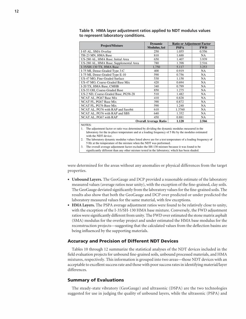
Table 8 lists the adjustment ratios for the unbound layers included in the field evaluation(Parts A and B), while Table 9 contains the ratios for the HMA layers. The adjustment ratios
Success Rates, % NDT Gauges Included in Field Evaluation Unbound Layers HMA Layers
Ultrasonic DSPA & PSPA 86 93 Steady-State Vibratory GeoGauge 79 ---
Impact/Penetration DCP 64 --- Deflection-Based LWD & FWD 64 56
Non-Nuclear Density EDG & PQI 25 71 GPR Single Air-Horn Antenna 33 54
Table 7. Success rates of the NDT devices for identifying physicaldifferences or anomalies.
Resilient Moduli, ksi Adjustment Ratios Relating
Laboratory Moduli to NDT ValuesProject Identification Laboratory
MeasuredValue
Predictedwith LTPPEquations
GeoGauge
DSPA DCP LWD
Fine-Grained Clay Soils Before IC Rolling 2.5 10.5 0.154 .0751 0.446 0.39 I-85 Low-
Plastic Soil After IC Rolling 4.0 13.1 0.223 0.113 0.606 0.39 NCAT; OK High Plastic Clay 6.9 19.7 0.266 0.166 0.802 --- SH-21, TX High Plastic Clay 26.8 19.6 1.170 0.989 3.045 2.78
Average Ratios for Fine-Grained Clay Soils 0.454 0.336 1.225 Embankment Materials; Soil-Aggregate Mixtures
South Embankment 16.0 15.7 0.696 0.367 1.053 3.13 TH-23, MN
North Embankment 16.4 16.3 0.735 0.459 0.863 3.13 US-2, ND Embankment 19.0 19.5 1.450 0.574 0.856 ---
SH-130, TX Improved Soil 35.3 21.9 1.337 1.029 1.657 1.43 Average Ratios for Soil-Aggregate Mixtures; Embankments 1.055 0.607 1.107
Aggregate Base MaterialsCo. 103, TX Caliche Base --- 32.3 1.214 --- 1.436 --- NCAT, SC Crushed Granite 14.3 36.1 0.947 0.156 --- --- NCAT, MO Crushed Limestone 19.2 40.9 0.747 0.198 --- ---
Crushed Stone, Middle 24.0 29.9 0.851 0.303 0.725 1.69 TH-23, MN
Crushed Stone, South 26.0 35.6 0.788 0.235 0.560 1.69 US-53, OH Crushed Stone 27.5 38.3 1.170 0.449 0.862 --- NCAT, FL Limerock 28.6 28.1 0.574 0.324 0.619 --- US-2, ND Crushed Aggregate 32.4 39.8 1.884 0.623 1.129 ---
US-280, AL Crushed Stone 48.4 49.3 1.010 0.244 0.962 1.04 Average Ratios for Aggregate Base Materials 1.021 0.316 0.899
Overall Average Ratios for Processed Materials 0.942 0.422 1.084 NOTES: 1. The adjustment ratio is determined by dividing the resilient modulus measured in the laboratory at a specific stress state by
the NDT estimated modulus. The overall average values listed above exclude those for the fine-grained clay soils. 2.
Table 8. Unbound layer adjustment ratios applied to the NDT moduli to representlaboratory conditions or values at low stress states.
12
were determined for the areas without any anomalies or physical differences from the targetproperties.
• Unbound Layers. The GeoGauge and DCP provided a reasonable estimate of the laboratorymeasured values (average ratios near unity), with the exception of the fine-grained, clay soils.The GeoGauge deviated significantly from the laboratory values for the fine-grained soils. Theresults also show that both the GeoGauge and DCP over predicted or under predicted thelaboratory measured values for the same material, with few exceptions.
• HMA Layers. The PSPA average adjustment ratios were found to be relatively close to unity,with the exception of the I-35/SH-130 HMA base mixture. Conversely, the FWD adjustmentratios were significantly different from unity. The FWD over estimated the stone matrix asphalt(SMA) modulus for the overlay project and under estimated the HMA base modulus for thereconstruction projects—suggesting that the calculated values from the deflection basins arebeing influenced by the supporting materials.
Accuracy and Precision of Different NDT Devices
Tables 10 through 12 summarize the statistical analyses of the NDT devices included in thefield evaluation projects for unbound fine-grained soils, unbound processed materials, and HMAmixtures, respectively. This information is grouped into two areas—those NDT devices with anacceptable to excellent success rate and those with poor success rates in identifying material/layerdifferences.
Summary of Evaluations
The steady-state vibratory (GeoGauge) and ultrasonic (DSPA) are the two technologiessuggested for use in judging the quality of unbound layers, while the ultrasonic (PSPA) and
Ratio or Adjustment Factor Project/Mixture DynamicModulus, ksi PSPA FWD
I-85 AL, SMA Overlay 250 1.055 0.556 TH-23 MN, HMA Base 810 1.688 NA US-280 AL, HMA Base; Initial Area 650 1.407 3.939 US-280 AL, HMA Base; Supplemental Area 780 1.398 2.516 I-35/SH-130 TX, HMA Base 1,750 5.117 3.253I-75 MI, Dense-Graded Type 3-C 400 0.919 NA I-75 MI, Dense-Graded Type E-10 590 0.756 NA US-47 MO, Fine-Graded Surface 530 1.158 NA US-47 MO, Coarse-Graded Base Mix 420 0.694 NA I-20 TX, HMA Base, CMHB 340 0.799 NA US-53 OH, Coarse-Graded Base 850 1.275 NA US-2 ND, Coarse-Graded Base, PG58-28 510 1.482 NA NCAT AL, PG67 Base Mix 410 0.828 NA NCAT FL, PG67 Base Mix 390 0.872 NA NCAT FL, PG76 Base Mix 590 1.240 NA NCAT AL, PG76 with RAP and Sasobit 610 1.3760 NA NCAT AL, PG76 with RAP and SBS 640 1.352 NA NCAT AL, PG67 with RAP 450 0.881 NA
Overall Average Ratio 1.128 2.566 NOTES:1. The adjustment factor or ratio was determined by dividing the dynamic modulus measured in the laboratory for the in-place temperature and at a loading frequency of 5 Hz by the modulus estimated with the NDT device.2. The laboratory dynamic modulus values listed above are for a test temperature of a loading frequency of 5 Hz at the temperature of the mixture when the NDT was performed.3. The overall average adjustment factor excludes the SH-130 mixture because it was found to be significantly different than any other mixture tested in the laboratory; which has been shaded.
Table 9. HMA layer adjustment ratios applied to NDT modulus valuesto represent laboratory conditions.

13
Statistical Value
Material Property NDT Devices StandardError
95%PrecisionTolerance
Pooled StandardDeviation
NDT Devices with Good Success Rates Based on Modulus or Volumetric Properties GeoGauge 2.5 4.9 1.1
Modulus, ksi DSPA 4.5 8.8 1.2
StructuralProperties
Thickness, in. None NA NA NADensity, pcf None NA NA NAAir Voids, % None NA NA NA
VolumetricProperties
StructuralProperties
VolumetricProperties
Fluids Content, % None NA NA NANDT Devices with Poor (or Undefined) Success Rates Based on Modulus or Volumetric Properties
DCP 3.8 7.4 1.9 Modulus, ksi
LWD/FWD 5.9 11.6 2.0 Thickness, in. GPR, single antenna NA NA NA
GPR, single antenna --- --- 4.2 Density, pcf
EDG 0.8 1.6 0.7 Water Content, % EDG 0.2 0.4 0.5
Table 10. NDT device and technology variability analysis for the fine-grainedclay soils.
Statistical Value
Material Property NDT Devices StandardError
95%PrecisionTolerance
Pooled StandardDeviation
NDT Devices with Good Success Rates Based on Modulus or Volumetric Properties GeoGauge 2.5 4.9 1.8
Modulus, ksi DSPA 4.5 8.8 1.5
StructuralProperties
Thickness, in. None NA NA NADensity, pcf None NA NA NAAir Voids, % None NA NA NA
Volumetric Properties
Fluids Content, % None NA NA NANDT Devices with Poor (or Undefined) Success Rates Based on Modulus or Volumetric Properties
DCP 3.8 7.4 5.3 Modulus, ksi
LWD/FWD 5.9 11.6 2.0 StructuralProperties
Thickness, in. GPR, single antenna 0.80 1.5 0.6 GPR, single antenna 3.4 6.7 3.0
Density, pcf EDG 1.0 2.0 0.8
VolumetricProperties
Water Content, % EDG 0.2 0.4 0.6
Table 11. NDT device and technology variability analysis for the processedmaterials and aggregate base materials.
Statistical Value
Material Property NDT Devices StandardError
95%PrecisionTolerance
Pooled StandardDeviation
NDT Devices with Good Success Rates Based on Modulus or Volumetric Properties StructuralProperties
Modulus, ksi PSPA 76 150 56
Density, pcf PQI & PT 1.7 3.4 2.5 Air Voids, % None NA NA NA
Volumetric Properties
StructuralProperties
Volumetric Properties
Fluids Content, % None NA NA NANDT Devices with Poor (or Undefined) Success Rates Based on Modulus or Volumetric Properties
Modulus, ksi FWD 87 170.5 55 GPR, single antenna 0.25 0.49 0.3
Thickness, in. GPR, multiple antenna 0.27 0.55 ---
Density, pcf GPR, multiple antenna 1.6 3.1 --- Asphalt Content, % GPR, multiple antenna 0.18 0.36 ---
GPR, single antenna 0.40 0.8 2.1 Air Voids, %
GPR, multiple antenna 0.22 0.4 ---
Table 12. NDT device and technology variability analysis for the HMA mixtures.

14
non-nuclear density gauges (the PaveTracker was used in Part B) are the technologies suggestedfor use of HMA layers. The GPR is suggested for layer thickness acceptance, while the IC rollersare suggested for use on a control basis for compacting unbound and HMA layers.
NDT Devices for Unbound Layers and Materials
• The DSPA and GeoGauge devices had the highest success rates for identifying an area withanomalies, with rates of 86 and 79 percent, respectively. The DCP and LWD identified abouttwo-thirds of the anomalies, while the GPR and EDG had unacceptable rates below 50 percent.
• Three to five repeat measurements were made at each test point with the NDT devices, withthe exception of the DCP.– The LWD exhibited low standard deviations that were less dependent on material stiffness
with a pooled standard deviation less than 0.5 ksi. One reason for the low values is that themoduli were less than for the other devices. The coefficient of variation (COV), an estimateof the normalized dispersion, however, was higher. It is expected that the supporting layershad an effect on the results.
– The GeoGauge had a standard deviation for repeatability measurements varying from 0.3to 3.5 ksi. This value was found to be material dependent.
– The DSPA had the lowest repeatability, with a standard deviation varying from 1.5 to21.5 ksi. The reason for this higher variation in repeat readings is that the DSPA sensor barwas rotated relative to the direction of the roller, while the other devices were kept stationaryor did not have the capability to detect anisotropic conditions. No significant differencewas found relative to the direction of testing for fine-grained soils, but there was a slightbias for the stiffer coarse-grained materials.
– The EDG was highly repeatable with a standard deviation in density measurements lessthan 1 pcf, while the GPR had poor repeatability based on point measurements. Triplicateruns of the GPR were made over the same area or sublot. For comparison to the other NDTdevices, the values measured at a specific point, as close as possible, were used. Use of pointspecific values from successive runs could be a reason for the lower repeatability, which areprobably driver specific. One driver was used for all testing with the GPR.
• The COV was used to compare the normalized dispersion measured with different NDT devices.The EDG consistently had the lowest COV with values less than 1 percent. The GeoGauge hada value of 15 percent, followed by the DSPA, LWD, DCP, and GPR. The GPR and EDG aredependent on the accuracy of other tests in estimating volumetric properties (density andmoisture contents). Any error in the calibration of these devices for the specific material isdirectly reflected in the resulting values, which probably explains why the GPR and EDGdevices did not consistently identify the areas with anomalies or physical differences.
• Repeated load resilient modulus tests were performed in the laboratory for characterizing anddetermining the target resilient modulus for each material. Adjustment ratios were deter-mined based on uniform conditions. The overall average ratio for the GeoGauge for the stiffercoarse-grained materials was near unity (1.05). For the fine-grained, less stiff soils, the ratiowas about 0.5. After adjusting for laboratory conditions, all NDT devices that estimate resilientmodulus resulted in low residuals (laboratory resilient modulus minus the NDT elasticmodulus). However, the GeoGauge and DCP resulted in the lowest standard error. The LWDhad the highest residuals and standard error.
• The DSPA and DCP measured responses represent the specific material being tested. TheDCP, however, can be affected significantly by the varying amounts of aggregate particles infine-grained soils and the size of the aggregate in coarse-grained soils. The GeoGauge measuredresponses are minimally affected by the supporting materials, while the LWD can be signifi-cantly affected by the supporting materials and thickness of the layer being tested. Thickness

deviations and variable supporting layers are reasons for LWD’s low success rate in identifyingareas with anomalies or physical differences.
• No good or reasonable correlation was found between the NDT devices that estimate modulusand those devices that estimate volumetric properties.
• Instrumented rollers were used on too few projects for a detailed comparison to the otherNDT devices. The rollers were used to monitor the increase in density and stiffness withincreasing number of roller passes. One potential disadvantage with these rollers is that theymay bridge localized soft areas. However, based on the results obtained, their ability of provideuniform compaction was verified and these rollers are believed to be worth future investmentin monitoring the compaction of unbound materials.
• The GPR resulted in reasonably accurate estimates to the thickness of aggregate base layers.None of the other NDT devices had the capability or same accuracy to determine the thicknessof the unbound layer.
NDT Devices for HMA Layers and Mixtures
• The PSPA had the highest success rate for identifying an area with anomalies with a rate of93 percent. The PQI identified about three-fourths of the anomalies, while the FWD and GPRidentified about one-half of those areas. The seismic and non-nuclear gauges were the onlytechnologies that consistently identified differences between the areas with and without seg-regation. These two technologies also consistently found differences between the longitudinaljoint and interior of the mat.
• The non-nuclear density gauge (PaveTracker) was able to identify and measure the detrimen-tal effect of rolling the HMA mat within the temperature sensitive zone. This technology wasbeneficial on some of the Part B projects to optimize the rolling pattern initially used by thecontractor.
• Three to four repeat measurements were made at each test point with the NDT devices.– The PSPA had a repeatability value, a median or pooled standard deviation, of about 30 ksi
for most mixtures, with the exception of the US-280 supplemental mixture that was muchhigher.
– The FWD resulted in a comparable value for the SMA mixture (55 ksi), but a higher valuefor the US-280 mixture (275 ksi).
– The non-nuclear density gauges had repeatability values similar to nuclear density gaugeswith a value less than 1.5 pcf.
– The repeatability for the GPR device was found to be good and repeatable, with a value of0.5 percent for air voids and 0.05 inches for thickness.
• The PSPA moduli were comparable to the dynamic moduli measured in the laboratory on testspecimens compacted to the in-place density at a loading frequency of 5 Hz and the in-placemixture temperature, with the exception of one mixture—the US-280 supplemental mixture.In fact, the overall average ratio or adjustment factor for the PSPA was close to unity (1.1). Thiswas not the case for the FWD. Without making any corrections for volumetric differences tothe laboratory dynamic modulus values, the standard error for the PSPA was 76 ksi (laboratoryvalues assumed to be the target values). The PSPA was used on HMA surfaces after com-paction and the day following placement. The PSPA modulus values measured immediatelyfollowing compaction were found to be similar to the values one or two days after placement—when making proper temperature corrections in accordance with the master curves measuredin the laboratory.
• A measure of the mixture density or air voids is required in judging the acceptability of themodulus value from a durability standpoint. The non-nuclear gauges were found to be acceptable, assuming that the gauges have been properly calibrated to the specific mixture—as for the PSPA.
15

16
• Use of the GPR single antenna method, even with mixture calibration, requires assumptionsthat specific volumetric properties do vary along a project. As the mixture properties change,the dielectric values may or may not be affected. Use of the proprietary GPR analysis methodon other projects was found to be acceptable for the air void or relative compaction method.This proprietary and multiple antenna system, however, was not used within Part A of the fieldevaluation to determine its success rate in identifying localized anomalies and physical differ-ences between different areas. Both GPR systems were found to be very good for measuringlayer thickness along the roadway.
• Water can have a definite effect on the HMA density measured with the non-nuclear densitygauges (PQI). The manufacturer’s recommendation is to measure the density immediatelyafter compaction, prior to allowing any traffic on the HMA surface. Within this project, theeffect of water was observed on the PQI readings, as compared to dry surfaces. The measureddensity of wet surfaces did increase compared to dry surfaces. From the limited testingcompleted with wet and dry surfaces, the PaveTracker was less affected by surface condition.However, wet versus dry surfaces was not included in the field evaluation plan for differentdevices. Based on the data collected within the field evaluation, wet surfaces did result in a biasof the density measurements with this technology.
• Another important condition is the effect of time and varying water content on the propertiesof the HMA mixture during construction. There have been various studies completed usingthe PSPA to detect stripping and moisture damage in HMA mixtures. For example, Hammonset al. (2005) recently used the PSPA (in combination with GPR) to successfully locate areaswith stripping along selected interstate highways in Georgia. The testing completed withinthis study also supports the use of ultrasonic-based technology to identify such anomalies.
• The instrumented rollers used to establish the increase in stiffness with number of passes wascorrelated to the increases in density, as measured by different devices. These rollers were usedon limited projects to develop or confirm any correlation between the NDT response andthe instrumented roller’s response. One issue that will need to be addressed is the effect ofdecreasing temperature on the stiffness of the mixture and how the IC roller perceives thatincrease in stiffness related to increases in density of the mat and a decrease in mat temperatureas it cools. A potential disadvantage with these rollers is that they will bridge segregated areasand may not accurately identify cold spots in the HMA mat. However, based on the resultsobtained, the ability to provide uniform compaction was verified and the rollers are believedto be worth future investments in monitoring the compaction of HMA mixtures.
Limitations and Boundary Conditions
• All NDT devices suggested for QA application, with the exception of the GPR and IC rollers,are point specific tests. Point specific tests are considered a limitation because of the numberof samples that would be required to identify localized anomalies that deviate from thepopulation.– Ultrasonic scanners are currently under development so that relatively continuous mea-
surements can be made with this technology. These scanners are still considered in theresearch and development stage and are not ready for immediate and practical use in a QAprogram.
– GPR technology to estimate the volumetric properties of HMA mixtures is available for useon a commercial basis, but the proprietary system has only had limited verification of itspotential use in QA applications and validation of all volumetric properties determinedwith the system.
– Similarly, the IC rollers take continuous measurements of density or stiffness of the materialbeing compacted. During the field evaluation, some of these rollers had both hardware and

software problems. Thus, these devices were not considered immediately ready for use in aday-to-day QA program. The equipment, however, has been improved and its reliability hasincreased. The technology is suggested for use on a control basis but not for acceptance.
• Ultrasonic technology (PSPA) for HMA layers and materials; suggested for use in control andacceptance plans.– Test temperature is the main boundary condition for the use of the PSPA. Elevated tem-
peratures during mix placement can result in erratic response measurements. Thus, thegauge may not provide reliable responses to monitor the compaction of HMA layers ordefine when the rollers are operating within the temperature sensitive zone for the specificmixture.
– These gauges need to be calibrated to the specific mixture being tested. However, this tech-nology can be used in the laboratory to measure the seismic modulus on test specimensduring mixture design or verification prior to measuring the dynamic modulus in thelaboratory.
– A limitation of this technology is that the results (material moduli) do not provide anindication on the durability of the HMA mixture. Density or air void measurements areneeded to define durability estimates.
– The DSPA for testing unbound layers is influenced by the condition of the surface. Highmodulus values near the surface of the layer will increase the modulus estimated with theDSPA. Thus, the DSPA also needs to be calibrated to the specific material being evaluated.
• Steady-state vibratory technology (GeoGauge) for unbound layers and materials; suggestedfor use in control and acceptance plans.– This technology or device should be used with caution when testing fine-grained soils at
high water contents. In addition, it should not be used to test well-graded, non-cohesivesands that are dry (i.e., well below the optimum water content).
– The condition of the surface of the layer is important and should be free of loose particles.A layer of moist sand should also be placed underneath the gauge to fill the surface voidsand ensure that the gauge’s ring is in contact with about 75 percent of the material’s surface.Placement of this thin, moist layer of sand takes time and does increase the time needed fortesting.
– These gauges need to be calibrated to the specific material being evaluated and are influencedby the underlying layer when testing layers that are less than 8 in. thick.
– These gauges are not applicable for use in the laboratory during the development of moisture-density (M-D) relationships that are used for monitoring compaction. The DSPA technologyis applicable for laboratory use to test the samples used to determine the M-D relationship.
– A relative calibration process is available for use on a day-to-day basis. However, if thegauge does go out of calibration, then it must be returned to the manufacturer for internaladjustments and calibration.
– These gauges do not determine the density and water content of the material. Alternatedevices are necessary to measure the water content and density of the unbound layer.
• Non-nuclear density gauges (electric technology) for HMA layers and materials; suggested foruse in control and acceptance plans.– Results from these gauges can depend on the condition of the layer’s surface—wet versus
dry. It is recommended that the gauges be used on relatively dry surfaces until additionaldata become available pertaining to this limitation. Free water should be removed fromthe surface to minimize any effect on the density readings. However, water penetrating thesurface voids in segregated areas will probably affect the readings (i.e., incorrect or highdensity compared to actual density from a core). The PSPA was able to identify areas withsegregation.
– These gauges need to be calibrated to the specific material under evaluation.
17

18
• GPR technology for thickness determination of HMA and unbound layers; suggested for usein acceptance plans.– The data analysis or interpretation is a limitation of this technology. The GPR data require
some processing time to estimate the material property. The time for layer thickness esti-mates is much less than for other layer properties.
– This technology requires the use of cores for calibration purposes. Cores need to be takenperiodically to confirm the calibration factors used to estimate the properties.
– Use of this technology, even to estimate layer thickness, should be used with caution whenmeasuring the thickness of the first lift placed above permeable asphalt treated base (PATB)layers.
– GPR can be used to estimate the volumetric properties of HMA mats, but that technologyhas yet to be verified on a global basis.
– Measurements using this technology cannot be calibrated using laboratory data.• IC rollers; suggested for use in a control plan, but not within an acceptance plan.
– The instrumented rollers may not identify localized anomalies in the layer being evalu-ated. These rollers can bridge some defects (may have insufficient sensitivity to identifydefects that are confined to local areas).
– Temperature is considered an issue with the use of IC rollers for compacting HMA layers.Although most IC rollers measure the surface temperature of the mat, the effect of temperature on the mat stiffness is an issue—as temperature decreases the mat stiffness willincrease, not necessarily because of an increase in density of the mat. Delaying the com-paction would increase the stiffness of the mat measured under the rollers because of thedecrease in temperature.
– The instrumented rollers also did not properly indicate when checking and tearing of themat occurred during rolling. The non-nuclear density gauges (PaveTracker) successfullyidentified this detrimental condition.
– Measurements using this technology and associated devices cannot be calibrated usinglaboratory data.
Conclusions
Unbound Layers and Materials
• The GeoGauge is a self-contained NDT device that can be readily incorporated into a QAprogram for both control and acceptance testing. This conclusion is based on the followingreasons:– It provides an immediate measure of the resilient modulus of the in-place unbound
material.– It identified those areas with anomalies at an acceptable success rate (second only to the
DSPA).– It adequately ranked the relative order of increasing strength or stiffness of the unbound
materials.– It provided resilient modulus values that were correlated to the dry density over a diverse
range of material types.– The normalized dispersion is less than for the other NDT devices that provide an estimate
of stiffness.– The training and technical requirements for this technology are no different than what is
required when using a nuclear density gauge.Two disadvantages of using this device in a QA program are (1) the need for measuring the
water content and density using other methods, which is also the case for the DSPA and other

modulus estimating devices and (2) the need to calibrate the test results to the material andsite conditions under evaluation. The latter is the more important issue and is discussed inmore detail.
The GeoGauge should be calibrated to the project materials and conditions to improve onits accuracy, especially when testing fine-grained soils. This calibration issue requires thatlaboratory repeated load resilient modulus tests be performed on each unbound layer forjudging the quality of construction. Most agencies do not routinely perform resilient modu-lus tests for design. Eliminating the laboratory resilient modulus tests from the calibrationprocedure will reduce its accuracy for confirming the design values, but not for identifyingconstruction defects. For those agencies that do not have access to or the capability to performresilient modulus tests, use of the FHWA-LTPP regression equations is an option that can beused to calculate the target resilient modulus at the beginning of construction. The targetresilient modulus should be the value used in structural design. For the MEPDG, this is theaverage value measured in the laboratory.
• The DSPA is also a self-contained unit that was successful in many of the areas noted for theGeoGauge. It was the device that had the highest success rate in identifying areas with differentphysical conditions or anomalies. An additional advantage of the DSPA is that the results canbe calibrated to the specific unbound material being tested prior to construction, when theM-D relationship is measured in the laboratory. This calibration procedure allows the DSPAto be used to detect volumetric, as well as physical, changes in the materials during construction.In other words, the DSPA modulus is measured on the M-D samples prepared at differentwater contents and dry densities. In short, the DSPA can be used in day-to-day operations toassist contractor and agency personnel in judging construction and materials quality by itselfor in tandem with other geophysical and/or ground truth sampling programs.
Two disadvantages of the DSPA are that it consistently resulted in a higher normalized dis-persion measured over a diverse range of conditions and materials, and that it requires moresophisticated training of technicians to correctly interpret the load pulse and responses toensure that satisfactory data have been collected by the device.
• The DCP was also successful in many of the areas noted for the GeoGauge. However, testingtakes much more time, especially for stiff materials and layers with large aggregate. In addition,the test results were found to be more dependent on aggregate size than the other NDT devices. The normalized dispersion was also found to be much higher than for the DSPAand GeoGauge.
Conversely, the DCP does have the capability to readily estimate the strength of thickerunbound layers and can measure the modulus gradient with depth. In fact, it can be used inconjunction with the GeoGauge and DSPA in adjusting the modulus values from those devicesto laboratory conditions for fine-grained soils for agencies that do not have resilient modulustesting capability in the laboratory. Use of the DCP can be considered an option in adjustingthe test results for the GeoGauge for those agencies that have no plans to incorporate a resilient modulus testing capability within their design or materials departments.
• The GPR (single antenna method) was found to have a poor success rate in identifying anom-alies. It did not provide a measure of modulus or strength of material. In addition, using thesingle antenna method requires that either the density or water content be assumed andthe other parameter calculated. Both vary along the project, resulting in higher variations ofthe property being calculated. Using an inaccurate value can lead to an incorrect finding. Forexample, the GPR found some of the areas tested to have the highest density, while most otherNDT devices found that area to be the softest and least dense. It was successful, however, inmeasuring the layer thickness of the unbound materials.
Two other disadvantages of this system are in the training requirements for using thistechnology and the need to calibrate the dielectric values to physical properties of the in-place
19

20
material. Samples need to be recovered and tested to determine the water contents and den-sities of those areas prior to using the results for QC or acceptance. This requires that controlstrips be used prior to construction, and these calibration factors should be checked periodicallyduring construction. Many agencies are not requiring control strips, or the first day of con-struction is the control strip. Training is another issue; this system requires more sophisticatedtraining for the operator to interpret the measurements taken with the GPR. Thus, with itscurrent limitations, it is not suggested for future use in testing unbound materials to determinethe quality characteristics of the in-place material. However, it is suggested that research withthe GPR continue because of its continuous coverage and speed of data collection.
• Similar to the GPR, the EDG was found to have a poor success rate in identifying areas withanomalies. However, this device is believed to have potential to provide volumetric data onthe unbound materials for use in a QA program with continued use. The density estimated fromthis device is definitely related to resilient modulus across a wide range of unbound materials.However, further improvements in the measurements will require a program to obtain addi-tional data. The variability of the water contents measured with this device was found tobe very low. Other agencies are beginning to use this device in their research programs. Forexample, Texas and Nevada have ongoing programs that could provide improvements to theequipment and procedures in the near future. As a result, further detailed evaluation of thisdevice and technology to improve its accuracy are warranted.
• The deflection-based methods (LWD and FWD) were found to have limited potential for QCpurposes. The LWD devices have greater mobility than the FWD, which is an advantage for theiruse over the FWD. These devices have more potential for use in acceptance programs of the finalstructure and certainly in forensic areas for evaluating the interaction between the pavementlayers and foundation. The following summarizes the conclusions reached on these devices:– Technology was unable to consistently identify those areas with anomalies.– The modulus values can be influenced by the underlying layers, resulting in lower or higher
and more variable modulus values.– The normalized dispersion was found to be high, relative to the other NDT devices.– The relationship between modulus from this technology and dry density was poor.– Any error in thickness of the layer being tested can result in large errors and more variabil-
ity that could lead to wrong decisions being made by the contractor and agency about theconstruction operation.
HMA Mixtures
• The PSPA is a self-contained NDT device that can be readily incorporated into a QA programfor both control and acceptance testing of HMA mixtures. As noted for unbound materials,an advantage of this technology is that the device can be calibrated to the specific materialsbeing tested during the mixture design stage for HMA mixtures. This calibration procedureallows the PSPA to be used to detect volumetric, as well as physical, changes in the materialsduring construction. In short, the PSPA can be used in day-to-day operations to assist con-tractor and agency personnel in judging construction and materials quality by itself or in tan-dem with other geophysical and/or ground truth sampling programs. This conclusion is basedon the following reasons.– The PSPA is the NDT device found best suited for QA applications because it adequately
identified all but one area with anomalies. The PSPA provides a measure of the dynamicmodulus that is needed for pavement structural designs, even before adjusting the PSPAmodulus for laboratory conditions. The PSPA modulus was found to be correlated to thedynamic modulus at elevated temperatures using the master curve developed from labo-ratory dynamic modulus tests.

– Similar PSPA modulus values were measured at higher temperatures and corrected fortemperature using a master curve in comparison to those measured in the laboratory.
– An important condition that the NDT device needs to consider is the effect of time andvarying moisture content on the properties of the HMA mixture near construction andhow those properties will change in service. There have been various studies completed onusing the PSPA to detect stripping in HMA mixtures. For example, the PSPA was used incombination with GPR to successfully locate areas with stripping along selected interstatehighways in Georgia (Hammons et al. 2005). The test results from the NCHRP 10-65 studysupport a similar conclusion.However, the PSPA does have some limitations regarding full-scale use in QA programs.
Use of the PSPA should be delayed after rolling to allow the mix to cool. Dr. Nazarian’s rec-ommendation is to delay all testing for one day after HMA placement and compaction. Ifrequired, this time restriction is considered a disadvantage for use in QA programs.
A measure of the mixture density or air voids is also required in judging the acceptabilityof the modulus value or durability of the HMA mixture. The two devices that deserve furtherevaluation include the GPR and non-nuclear density gauges. The GPR provides full coveragein a short period of time.
• The non-nuclear density gauges are also well suited for QA because they can be readily incor-porated into control programs. Some contractors are already using the non-nuclear densitygauges in controlling the compaction operation. This technology was also used to identifyanomalies at a reasonable rate and can be used to identify tender mixtures and the effects ofrolling in the temperature sensitive zone.
Variations in water have a definite effect on the HMA density measured with the PQI. Themanufacturer’s recommendation is to measure the density immediately after compaction,prior to allowing any traffic on the HMA surface. This type of time restriction is considered adisadvantage to the use of the PQI in a day-to-day practical QA program. This time effect,however, was not found within the Part A test program, but the moisture effect was observedin Part A of the field evaluation. Use of other non-nuclear density gauges (PaveTracker) didnot exhibit this moisture sensitivity. However, the effect of water on these gauges was notincluded in the field evaluation as a primary variable. Measurements were taken after heavy rainsin areas where the readings were previously taken prior to the thunderstorms. The same densityvalues were measured after removing and drying all free water at the surface. This potentialbias of free water on the surface is not considered a limitation but must be considered in takingmeasurements for control purposes.
• Use of the GPR technology using the single antenna method, even with mixture calibration,requires assumptions on specific volumetric properties that do vary along a project. Using themulti-antenna method is expected to improve on the measurement of the volumetric prop-erties and identification of areas with deficiencies or anomalies. Thus, the GPR is suggestedfor continued research studies, especially with the multiple antenna system, which is a propri-etary analysis system. The proprietary system needs additional validation prior to full-scaleimplementation into a QA program.
• The FWD is not suggested for use in QA programs, because this technology was unable toidentify some of the anomalies. In addition, the FWD has high variation in elastic modulusvalues, and those values are influenced by the strength of the underlying materials and layers.
Recommendations
The research team’s recommendations are based on the evaluation of NDT devices for imme-diate and practical use in QA programs. Thus the GeoGauge can be used for estimating themodulus of unbound layers, while the PSPA is the device suitable for use with HMA layers.
21

22
The PaveTracker can be used in establishing and confirming the rolling pattern for HMA mix-tures. Other NDT devices may provide useful data for pavement and materials testing purposes.Each has its own benefits and advantages for evaluating and designing pavements.
The IC or instrumented rollers can be valuable to a contractor in terms of controlling the com-paction operation. These rollers that operated without problems were used on too few projectsto suggest their immediate inclusion in QA programs. Nonetheless, they can assist the contractorin optimizing the compaction of the material. Their disadvantage for HMA layers is the temper-ature of the mat issue. Decreases in temperature will cause the stiffness of the mat to increase.Thus, other devices still need to be used with the IC rollers for control. The use of IC rollers foracceptance is not suggested at this time.
Research with the multi-antenna GPR device and proprietary data interpretation systemshould not be abandoned and should be validated in future studies. This system definitely showspromise in providing the volumetric properties for HMA mixtures. The data can be collected athighway speeds, and the proprietary data interpretation system can provide results on a real-timebasis. The disadvantage of this system is that it also needs field cores for calibrating the methodto project specific conditions. These cores should be taken periodically to confirm the calibra-tion factors being used in estimating the volumetric properties.

23
The research team submitted the following chapters as Part III—Data Interpretation andApplication. This part is published herein as Chapters 1, 2, and 3 of NCHRP Report 626. Thechapters describe the physical characteristics and process for using each NDT technology anddevices on construction projects to define construction quality. Each system was evaluated intwo parts: (1) the system’s potential to be integrated into the flexible pavement constructionprocess (level of process impact) and (2) the reliability and accuracy of the system (system accu-racy and reliability). Chapter 1 focuses on the level of process impact on construction. In otherwords, what impact will the device have on the contractor’s progress, and will agencies need sub-stantially more staff to use the technology? Chapters 2 and 3 focus on the system accuracy andreliability of the different technologies and devices included in the field evaluation study.
Data Interpretation and Application

24
Some NDT devices initially were operated by a representa-tive of the manufacturer and then used by field technicians orengineers. Those devices that were found to have a reasonablesuccess rate in identifying anomalies were used by the con-tractor and agency staff in their daily QA operations, in accor-dance with manufacturers’ guidelines. Clustered tests wereperformed using each NDT device to determine the repeata-bility and accuracy of each system in evaluating its effective-ness in defining construction quality. The time and personnelrequirements to perform each test were recorded. This infor-mation was considered in rating the level of impact that eachdevice may have on construction. Since the technology was ofprimary interest (not a particular system or manufacturer),reports on each system are presented under the heading of thetechnology used by the system.
1.1 Ultrasonic—PSPA and DSPA
This system is applicable to HMA, unbound aggregatebase, and embankment soils. The PSPA is used to test HMA,while the DSPA is used for unbound materials and soils. Bothdevices consist of a stand linearly connected by a stiff arm toa source and two receivers and by wire to a computer, as shownin Figure 2. The source contains a hammer which is droppedseveral times at regular intervals. The receivers, containingquartz-crystal accelerometers, measure the acceleration of theRayleigh waves induced by the dropping of the hammer andreport the resulting electrical charge to the data acquisitionsystem. An FFT transforms the electrical charge or data intothe frequency domain. There is also a temperature sensor inthe system. Sturdiness of the laptop is an important feature.
The PSPA test can be and was performed on cold materialone or multiple days after placement, as well as on surfacesat elevated temperatures immediately after compaction. Thesystem’s temperature gauge is used to incorporate the tem-perature into the calculation of the material’s modulus. Therubber pads beneath the receivers deteriorate more rapidly
when used on surfaces at elevated temperatures. In fact, theyhave been known to melt when used on HMA surfaces shortlyafter placement. The operator needs to check these periodi-cally to ensure adequate coupling between the receivers andthe surface. These pads are easily replaced.
Both devices work properly as long as all points are in firmcontact (coupled) with the surface being tested. Adequate cou-pling is the system’s primary limitation. The speed of datacollection makes this technology a good candidate for QCapplications, assuming that the temperature of the material is properly considered by the modulus calculation process.None of the PSPA and DSPA devices (including the laptops)used exhibited any problems. The main operational issue wasinspecting and replacing the rubber pads of the receivers toensure good contact with the surface being tested.
The data interpretation program that comes with the PSPAand DSPA devices uses this information to provide the outputin the form of the mean Young’s modulus to a particulardepth. The spacing of the receivers determines the depth ofmeasurement. The operator needs to be trained to visuallyinspect the load pulse and response data on the output screenfor judging the suitability of an individual test (see Figure 3).This training is considered more sophisticated than what isrequired for a nuclear density gauge. The operator also needsto ensure that the spring-loaded receivers are in contact withthe surface between each test. If one of the receivers getsstuck, the result will be a data anomaly or “false” reading.With proper training, the operator can easily identify falsereadings by viewing the shape of the load pulse and receiverresponse. The shapes of the load pulse and receiver responseare visually displayed on the laptop screen for each reading.
The PSPA is used to test HMA mixtures, while the DSPA isused to test crushed aggregate base layers, embankments, andprepared subgrades. The DSPA was used on the shoulders ofthe US-280 reconstruction project instead of on the mainroadway because the roadway base layer had been chip-sealed.This type of surface reduces the repeatability of the ultrasonic
C H A P T E R 1
Applicability of NDT Technologies on Construction Projects

device, as well as other NDT devices, because the points of thereceivers and source are not always in good contact with thesurface tested. Ensuring good contact with the surface beingevaluated is important for both the PSPA and DSPA.
The system initially converts the readings of the load pulseand response to a seismic modulus of the material. The seismicmodulus is internally adjusted to a modulus at a specific con-dition (temperature and load frequency for HMA). Each testlocation requires three to five tests for this system. Each testtook 10 to 20 seconds to complete. Therefore, the entire process(3 to 5 readings at a point) takes only slightly longer than thesystem currently used for QC, the nuclear density gauge,which is generally set for one 60-second reading.
This system can also be used to estimate the elastic proper-ties parallel and perpendicular to the direction of the rollers(refer to Chapters 2 and 3). Measuring the seismic propertiesin different directions actually increases the perceived vari-ability of the device. The variability can be reduced slightly byalways taking the readings in one direction. All other NDTdevices result in an average or equivalent value at a test point.
The spacing of the receivers can also be changed easily fortesting thin and thick layers. Layer thickness variation thatoccurs along a construction project can have less of an impacton the resulting seismic modulus values than on the resultingvalues from other NDT technologies.
Another advantage of this technology is that the system canbe calibrated easily to the specific materials being tested duringthe mixture design stage for HMA materials or in developingM-D relationships for unbound materials. This calibrationprocedure allows the PSPA and DSPA to be used to detectvolumetric, as well as physical, changes in the materials duringconstruction.
The DSPA can be used to develop modulus growth withcompaction relationships during the first day of constructionfor the unbound layers and periodically during the project.Use of the PSPA to develop HMA modulus growth relation-ships can be problematic because of the elevated temperature.It is more applicable to warm-mix projects.
The equipment (including the laptop) was found to bedurable, and it did not require more personnel than those now
25
Carriage case recently developed for facilitating the use of thePSPA & DSPA in data collection.
Figure 2. PSPA in operation for testing HMA layers. The DSPA is used for testingunbound layers.

being used for control or acceptance of flexible pavement con-struction. In fact, the same technician using the nuclear densitygauges or taking cores from the HMA layer could also operatethe PSPA and DSPA at the same time. Its main disadvantage istraining the operators to determine a “false” reading.
In summary, the ultrasonic technology can be used in day-to-day QA operations to assist contractor and agency personnelin judging construction and materials quality by itself or intandem with other geophysical and/or ground truth samplingprograms.
1.2 Steady-State Vibratory—GeoGauge
This system is applicable to HMA and unbound materialsand soils, and is similar to the roller-mounted devices thatare described in Section 1.7. The GeoGauge, however, is onlyused for testing unbound materials and soils. The GeoGaugeprovides elastic modulus values that are displayed on thegauge or stored in the device and downloaded to a computerat a later date. The resulting values were found to be similarto the resilient modulus values measured in the laboratoryor calculated from the resilient modulus regression equa-tions developed through the FHWA-LTPP program (Yauand Von Quintus 2002). The elastic modulus values from the
GeoGauge were found to be a function of the material’smoisture content and density. Stiffness readings were alsoreported by the test equipment and were a function of thestructure.
The process followed by the GeoGauge operator is almostidentical to that followed by an operator of the current state-of-the-art nuclear density gauge, except that the GeoGaugeoperator spreads a thin layer of sand on the pavement surface toset the instrument on before taking the reading (see Figure 4).The operator clears the surface to be tested with a small broomor other device to remove loose surface particles (see Figure 4).A thin layer of moist sand is used on rough surfaces to fill insurface voids to ensure that the ring under the gauge is in con-tact with at least 75 percent of the test surface. Moist sandshould be used because the gauge vibrations will cause drysand particles to shift under the gauge and disturb the reading.The layer of moist sand should only be thick enough to fill thesurface voids of the material being tested. A light pressure androtation of the GeoGauge was also used to ensure good contactwith the test surface.
Each test takes 75 seconds, as compared to the nucleardensity gauge’s 60 seconds. Thus, this test takes about twiceas long as the nuclear density gauge, including the time forspreading the sand. The test procedure is still quick enoughnot to be a hindrance to the contractor’s progress and does
26
Figure 3. DSPA and PSPA being used to test different materials.

not require more personnel than those now being used forcontrol and acceptance. As for the DSPA, the same technicianusing the nuclear density gauge or running sand-cone testscould also operate the GeoGauge at the same time. The train-ing and technical capability of the operator is no more thanwhat would be required for operating a nuclear density gauge.
Similar to the DSPA, the GeoGauge can easily be used todevelop relationships between modulus growth and com-paction effort in unbound layers. Such relationships can be initially developed at the start of the project to optimizethe compaction process and then be periodically verifiedthroughout the project. This feature becomes advantageouswhen the water content significantly varies from the optimumvalue measured in the laboratory.
The GeoGauge should be calibrated to the project materialsand conditions to improve on its accuracy, because of thepotential influence of the supporting materials. This calibrationissue requires that laboratory repeated load resilient modulustests be performed on each unbound layer for judging thequality of construction. Most agencies do not routinely per-form resilient modulus tests for design or for forensic evalu-ations, even though the 1993 AASHTO Design Guide suggeststhat they be performed (AASHTO 1993). Eliminating thelaboratory resilient modulus tests from the calibration proce-dure will reduce its accuracy for confirming the design values,
but not for identifying construction defects. As a replacementto the repeated load resilient modulus test, the regressionequations developed from repeated load resilient modulustests included in the LTPP program (Yau and Von Quintus2002) or the use of the DCP is permissible.
The disadvantage of the GeoGauge is that it will result inhigh variability when testing non-cohesive, well-graded sandsor similar soils. In addition, the elastic modulus readings fromthe gauge represent an equivalent modulus for the upper 10 to12 in. of the layer. Thus, the gauge in its current form shouldnot be used to test thin (less than 4 in.) or thick (greater than12 in.) layers without proper material calibration adjustmentsor changing the diameter of the ring under the gauge.
In summary, the GeoGauge has potential use in day-to-dayQA programs by both the contractor and the agency personnel.
1.3 Deflection-Based Methods
1.3.1 Falling Weight Deflectometer
The FWD is a large, expensive apparatus that is mountedon a trailer and pulled behind a tow vehicle. The operatorworks a computer and locates the apparatus for testing (seeFigure 5). This system is capable of applying dynamic loadsto the pavement surface, similar in magnitude and duration to
27
Figure 4. Humboldt GeoGauge.

that of a single heavy moving wheel load. It is being used withinthe LTPP program, and most state agencies have access to atleast one FWD. Thus, it is already being used in most agencies’day-to-day practice.
The response of the pavement system is measured in termsof vertical deformation, or deflection, over a given area usingseismometers or geophones. An FWD enables the user to deter-mine a deflection basin caused by a controlled load. Theseresults make it possible to determine the stiffness of existingpavement structures for use in M-E based rehabilitation designmethods.
The falling weight strikes a set of rubber buffers mountedto a 300-mm circular foot plate, which transmits the force tothe pavement (see Figure 5). A thin-ribbed rubber pad is alwaysmounted under the footplate. By varying the mass or the dropheight or both, the impulse load can be varied. This load maybe varied between 10 kN and 140 kN. Sensors measure thesurface deflections caused by the impulse load.
Most agencies use seven sensors at the spacing recommendedby LTPP. However, fewer or more sensors can be used, andthose can be spaced uniformly or at some other spacingselected by the user. Peak deflections are recorded, stored, and
displayed. In some cases, one of the geophones or sensors canbe incorrectly placed on the test surface by the sensor bar,especially on rough surfaces. The data acquisition softwarewill identify this anomaly, notifying the operator that the testshould be rejected and redone.
The test takes about 2 minutes to complete, including theuse of seating drops. Seating drops are important and shouldbe used at each test point. This does not include time to con-figure the trailer and set up the data acquisition system, whichshould only have to be done once per day for each project. Ittakes about 30 minutes to configure the trailer and 2 to 3 min-utes to set up the data acquisition program. Similar to thePSPA, the operator needs more technical and sophisticatedtraining in setting up the equipment and visually interpretingthe deflection basin data.
A separate data interpretation system or software is requiredfor producing elastic modulus values from the measureddeflection basins—Young’s modulus for each layer. Thecalculated elastic modulus values are structure dependent.Most data interpretation or analysis programs used back-calculation techniques for calculating layered elastic modulusvalues. Backcalculation programs do not determine unique
28
Figure 5. Trailer mounted FWD.

modulus values for each layer and are sensitive to layer thick-ness variations. Forward-calculation procedures have beendeveloped that result in unique layer modulus values for aparticular deflection basin, but these values are thicknessdependent. Any errors in the layer thickness will increase theerror and variability of the processed data.
Its use for acceptance of individual layers by the agencyshould be limited to the use of the forward-calculation proce-dure. Because the backcalculation procedures do not result inunique layer modulus values, it would be difficult to defend incontractor disputes where material has been rejected or pay-ment penalties issued to the contractor. The device can be usedto check or confirm the final flexible pavement for new con-struction or HMA overlays of existing pavements, but wouldprobably create many disputes with the contractor when theentire pavement structure is rejected at the end of the project.
In addition, the resulting values for the upper layer aredependent on the stiffness and variability of the supportinglayers. Calculating the elastic modulus of layers is generallyrestricted to those that are thicker than 3 in. The FWD mayalso require one additional field technician and tow vehicle.
The expense, size of the system, time needed to performeach test, and data interpretation software make this systemless practical for QC and acceptance. Thus, the FWD is believedto be less practical and effective for the QA uses that are thefocus of this study.
1.3.2 Light Weight Deflectometer
The LWDs use the same theory as the FWD, but offer anadvantage of being much more portable. In addition, thetraining and technical requirements for the LWD operatorsare no different than for nuclear density gauges, with oneexception—the operator needs to understand and be awareof the factors and physical features that affect layer moduluscalculated from the measured deflections. Results from theLWDs were significantly influenced by the supportingmaterials on some of the projects.
All three LWD devices used on selected projects havesimilar features. Only the Dynatest and Carl Bro devices arediscussed in the following paragraphs.
1.3.2.1 Dynatest Prima 100 LWD Device
The Prima 100 is manufactured by Dynatest and consistsof the weight (hammer) on a pole and the sensors (geophones)in a plate on the ground, all encompassed in one, connected,portable structure (see Figure 6). The sensors were connectedto a handheld computer by wireless remote technology.
The unit tested was somewhat flexible and the frame cameapart on multiple occasions. Besides slowing down the process,this resulted in questionable data because the wireless remote
would sense the jolt from the frame coming apart as a sepa-rate test, resulting in a deflection and modulus value for thatanomaly.
The wireless remote was troublesome and kept losing con-tact with the apparatus. This happened anytime the techniciancarrying the apparatus came within a few feet of the technicianholding the computer. This slowed down the operation becausethe computer had to be re-started each time it occurred.
When using the system on particularly stiff base material, thehammer can bounce high enough, such that it can strike theapparatus again—resulting in an appreciable rebound load.The rebound load can cause the remote to mistake that reboundas a second or separate test. The software, as written, causes theactual test results to be deleted and replaced by a reading of therebound.
The system, however, is fast. One test takes about 10 seconds,so the five tests conducted (and averaged) at each locationtake approximately the same amount of time that a nucleardensity reading takes at one location. However, the apparatusis bulky to handle, so the time that most non-nuclear systemsgain by not having to deal with the steps of transporting thenuclear device are lost.
29
Figure 6. Dynatest Prima 100 LWD.

1.3.2.2 Carl Bro LWD Device
The Carl Bro system looks exactly like the Dynatest system,except that it has additional sensors that are not attached tothe frame. These extended geophones do not change the theoryand applications. Although, the algorithms are slightly differ-ent to include input from the additional sensors, the theoryand application appear to be the same.
The geophones are arranged linearly at set distances fromthe plate. Since the sensors are connected to each other by a bar,but separate from the loading plate, connecting and placingthem at a specific distance from the plate for each test becomesproblematical. It is expected, however, that these perceiveddisadvantages can be resolved in future modifications to theequipment.
The process, from the beginning through the last of the fivedrops, takes an average of about 5.5 minutes. The procedurefollowed for using the system is listed.
1. Locate test point (surface must be even (flat) and must becleared of anything that could cause part of the plate tolose contact with the surface).
2. Set the loading plate on the surface to be tested (plate mustbe flat on the surface).
3. Measure for geophone location.4. Set the geophone arm and line up the sensors.5. Set data acquisition key for collecting the deflection data.6. Drop hammer (first drop “seats” the plate and is not read).7. Repeat last two steps for five drops at each location
(including the one to seat the plate).
This system had a wired connection to a laptop computerand was more cumbersome to set up because of the additionalgeophones. In addition, the seating drop of the plate some-times moved the plate. This increased the variability in the datagathered from the geophones and increased the number ofanomalies. The system is comparable in cost to the Prima 100.
1.3.2.3 Summary
This technology was tested on crushed aggregate basematerial, embankments, and prepared subgrades. However,there should be no difference between the procedures and thedevice’s reaction to a hard base material and those of HMAmixtures. A key advantage of this technology is that it givesthe operator a reading of the elastic modulus in about thesame time required to obtain a nuclear density gauge reading.The disadvantages are that the devices have limited reliabilitybecause of the range and reliability of the wireless remote andits software logic. In addition, the resulting values for theupper layer are dependent on the stiffness and variability ofthe supporting layer.
It is expected that these disadvantages of the equipmentcan be easily resolved with future modifications. These deviceswill likely make the technology and device more expensive. Itdoes, however, provide the agency with elastic modulus val-ues that can be used to confirm design assumptions withproper calibration. In summary, the LWDs are believed to beless practical and effective for the uses that are the focus ofthis study.
1.4 Dynamic Cone Penetrometer
The DCP is used to estimate the strength and modulus ofunbound materials and soils. The DCP is much like the LWDin appearance (see Figure 7); however, it uses a 15-lb (6.8-kg)steel mass falling 20 in. (50.8 cm) that strikes the anvil to causepenetration of a 1.5-in. (3.8-cm) diameter cone (45° vertexangle) that has been seated at the surface or in the bottom ofa hand augered hole (see Figure 8). The blows required to drivethe embedded cone a depth of 13⁄4 in. have been correlated byothers to N values derived from the Standard PenetrationTest (SPT). Experience has shown that the DCP can be usedeffectively in augered holes to depths of 15 to 20 ft (4.6 to 6.1 m).The system has been used in the past for the testing of soilsmore than anything else.
The technical skills and training requirements for the DCPoperator are no different than for a nuclear density gauge.Advantages of the DCP include its simplicity, low maintenance(using disposable tips, making sure that the allen screws are kept tight, etc.), mobility, and low cost. It can also be usedto test thick embankment layers, unlike some of the otherNDT technologies and devices.
Conversely, the manual apparatus is slow (tests took 5 to10 minutes at each location), its use is physically demanding,and the test is actually destructive to bases and pavements,that is, the test creates a hole in the material. Use of thedevice can also be dangerous, if the operator’s hand gets caught
30
Figure 7. DCP before assembly for use in measuringthe in-place strength of unbound materials and layers.

between the hammer and base for the hammer. Furthermore,soils or materials with boulders or large aggregate particles(refer to Figure 9) can cause refusal of the device. When thisoccurs, the test point should be moved and the test redone.An automated trailer mounted DCP is available, but is moreexpensive (see Figure 10). Only the manual DCP was used inthe field evaluation of NCHRP Project 10-65.
The manual DCP is considered to have potential for QCuse on a day-to-day basis, but an additional contractor andagency staff person would probably need to be assigned to usethe DCP under normal practices; however, the training andmaintenance of this device is considered minimal.
1.5 Ground Penetrating Radar
GPR is a pulse echo method for measuring pavement layerthicknesses and properties. GPR uses radio waves to penetratethe pavement by transmitting the wave energy into the pave-
ment from a moving antenna. These waves travel through thepavement structure and echoes are created at boundaries ofdissimilar materials. An air-coupled horn antenna attachedto the back of a small SUV (see Figure 11) was used in thefield evaluation of NCHRP Project 1065 to evaluate HMA,unbound aggregate base, and embankment soils.
The speed of data collection is one of the biggest advan-tages of GPR technology. There should be no impact to thecontractor’s operation, because this system collects the sameinformation regardless of material temperature and is capa-ble of taking measurements at speeds of up to 40 miles perhour. Higher speeds have been used on more recent projectsthrough enhancements made to the equipment and dataacquisition systems. The disadvantages of the technology arethe interpretation of the dielectric values that are measuredand personnel requirements for calibrating and maintainingthe equipment and data interpretation software.
The system is simple to operate and provides results imme-diately, at least in terms of dielectric values. The results are inthe form of a “picture” of the pavement system, much like anX-ray. Although the transducer is located above the surface,aimed downward, the picture can be viewed from “plan” or“elevation” (“profile”) perspective. Another huge advantageof this technology is that a continuous profile of the dielectricvalues is available. In fact, layer thickness profiles or completecontours of the layer can be developed in a short time period.
Currently, the technology requires operators with specialtechnical skills to interpret the data that have physical meaningto the quality of construction. Software programs are avail-able that provide color-coded charts and contours of thematerial. This system has been used to determine layer thick-ness at a reasonable accuracy—when layers with differentdielectric values are tested. The accuracy of the analysis pro-grams requires cores to accurately measure the in-place thick-ness and other volumetric properties.
Most of the data reduction-presentation programs, how-ever, still require some volumetric properties to be assumedin estimating density, air voids, and other volumetric prop-erties. These assumptions result in error of the properties thatare calculated from the dielectric values. The assumptionsare believed to be a reason why the GPR’s analysis and inter-pretation from the Part A projects did not coincide with someof the other NDT devices. There are programs available thatdo not require many assumptions, but all of the known pro-grams are proprietary. These proprietary programs werenot used in the Part A field evaluations, but were includedin the Part B summary at a few facilities. Data from some ofthese proprietary programs is presented and discussed inChapter 2.
Calibration is another issue that is important to the suc-cess of GPR antennas in estimating volumetric propertiesof materials. Cores have to be recovered and the physical
31
Figure 8. Manual DCP in operation (courtesy of Minnesota Road Research Section, Office of Materials,Minnesota DOT).

32
Large aggregate particles in the embankment soil caused refusal of the DCP in localized areas. These particles
found near the surface also had an impact on the DSPA and GeoGauge readings.
Figure 9. DCP test and large aggregate particles encountered at some of the projects, resulting in refusal of the test.
Figure 10. Automated DCP attached to a trailer (courtesy of Minnesota RoadResearch Section, Office of Materials, Minnesota DOT).

properties of those cores determined and correlated to thedielectric values measured by the GPR prior to and duringconstruction. This requires that control strips be used at thebeginning of a project and the correlations periodically con-firmed during construction. Many agencies are eliminatingor not requiring the contractor to use control strips, especiallyfor small projects. Thus, this technology has limited use inQC applications, but has greater potential for use in accept-able programs—especially those for which thickness is includedin the price adjustments or pay factors.
1.6 Electric Current/ElectronicMethods
This family of systems includes those that rely on technologysuch as electrical sensing fields, impedance, electric current,and radio waves to determine the quality of HMA pavement,base, or embankment (see Figures 12 and 13). The trainingand technical skills required to operate this technology are nodifferent than those required for nuclear density gauges. Inaddition, the calibration requirements to improve on the accu-racy of testing specific materials with the non-nuclear gaugesare similar in detail and extent for nuclear density gauges.
1.6.1 Electrical Density Gauge
An electrical density gauge was used in the Part A fieldevaluation projects, because of the equipment’s perceived easeof use and application to a diverse set of unbound materialsand soils. The specific gauge used was the one manufactured
33
Figure 12. Electrical density gauge.
b. Ground-Coupled Antenna Arrays Attached to Survey Vehicle
GPS Receiver
GPR Antenna
a. Air-Coupled GPR Antenna Attached to Survey Vehicle
GPS Data Acquisition& Storage
Figure 11. GPR antennas attached to a standard survey vehicle.

by EDG, which is confined to use on aggregate base layers,embankments and subgrades, or any unbound layer (see Fig-ure 14). The system uses 6-in. darts that are driven into thesoil within a 1.8 square foot area. This allows the system tomeasure a 1.0 cubic foot volume of material.
The system uses a 3-MHz radio signal, producing a currentof a certain voltage and phase, which allows measurements ofthe capacitance, resistance, and impedance. The connecteddata acquisition program uses algorithms and ratios of themeasured parameters to determine the density and watercontent of an unbound layer (refer to Figure 14).
This test takes several minutes to perform, but it appears tohave huge potential for use in replacing the nuclear densitygauges and other traditional QA tests, such as the sand-cone
tests. This technology does not require more personnel thanare now being used for QC/QA of unbound layers. The systemand devices should be easier to maintain and the operators ofthe equipment can be easily trained in its use—similar to anuclear density gauge.
The most time-consuming but critical part of the system isdeveloping a proper soil model for density and moisturecontent measurements. To date, other more traditional tests(such as sand cones) are performed in specific locations thatcover the range in density and water contents. A regressionmodel is then developed based on correlations between theEDG values and the density and water contents measuredfrom other tests. It is expected that this test will be improvedwith time, but at present, its use as a practical device for con-trolling construction of unbound layers is limited.
1.6.2 Pavement Quality Indicator
The PQI (see Figure 15[a]) uses a constant voltage, radio fre-quency, electrical impedance approach, in which a toroidalelectrical sensing field is established in the material being tested.This allows the PQI to make quick, in-situ measurements ofpavement density. The sensor consists of a set of flat plates thatare interconnected to form the electrodes of a planar capacitor.Variations in density are determined through changes in thedielectric constant of the medium between the capacitor plates.
Using this technology, the PQI can be used like the nucleardensity gauge, with the exception that it has the capability toadjust for moisture variations and mix type. The device alsohas an onboard, real-time system that takes the readings andkeeps a record of them, allowing it to be integrated seamlesslyinto the paving process.
1.6.3 PaveTracker
The PaveTracker (see Figure 15[b]) is a light weight non-nuclear device for measuring the uniformity of HMA mixtures.The measurements are practically instantaneous when thedevice is placed on an HMA surface. Areas of segregation,lower density levels along longitudinal joints or other non-uniformity areas can be detected by the PaveTracker Plus,which allows the operator to correct the problem before con-struction is complete.
The advanced software, built-in reference plate, and enlargeddisplay screen are some of the features offered by the Pave-Tracker. The large display screen is an advantage, becausethe device is compact and close to the ground. Like the PQI,the PaveTracker can be used exactly like the nuclear densitygauge, without the use of any nuclear device. The PaveTrackeralso has an onboard, real-time system that takes the densityreadings and keeps a record of them for future use, allowingthe device to be easily integrated into the paving process.
34
Figure 13. Purdue TDR method (courtesy of DurhamGeo website).
Figure 14. Electrical density gauge in the field.

1.7 Intelligent Compactors/Rollerswith Mounted ResponseMeasuring Devices
These systems offer real-time pavement quality measure-ment with no negative impact to the contractor’s progress.They use accelerometers to measure parameters of the com-pactor’s vibratory signature. Other sensors are also used togain information about the pavement. Information from thesensors is then used to make decisions about pavement quality.Although these roller-mounted systems have been shownto be beneficial to a contractor from a control standpoint,they have not been used for acceptance and confirmationof the design-modulus values. Two of these systems wereused in the demonstrations sponsored by FHWA at theNCAT and MnROAD facilities and included in the NCHRPProject 10-65 field evaluations. They are described in thefollowing paragraphs.
1.7.1 Asphalt Manager and Varicontrol System
This system, developed by Bomag, contains an onboardpavement analysis system based on the electrical charge gen-erated by strategically mounted quartz-crystal accelerometersthat measure the acceleration of the vibratory drums of thecompactor. An onboard computer transforms the data fromthe sensors using an FFT into the frequency domain. Thistransformation allows the computer to calculate the material’s
modulus. There is also a temperature sensor in the system,which feeds data into the computer for use in modulus calcu-lations. In addition, the system takes this reading and altersthe compaction effort of the roller to avoid the damaging effectsof over-compaction. Stiffness readings are taken continuouslyand presented as a modulus value developed by Bomag andcalled Evib, in the form of MN/m2.
The Evib value should be related to the dynamic modulus ofthe material being compacted. However, this computed valueis expected to be affected by the underlying support conditions.To date, the Evib value has not been evaluated or checked againstdynamic modulus values measured in the laboratory or esti-mated through other NDT devices.
The system is fully integrated into a vibratory roller that ispart of an operational paving train (see Figure 16). The true testof this “intelligent compaction” system is whether it actuallysaves time (fewer passes), improves uniformity of the mat,and renders accurate, consistent readings. As for this part of theanalysis (impact on the contractor’s progress), assuming thatthe system does what it claims, it can only help the contractor’sprogress.
1.7.2 Ammann Compaction Expert
Ammann-America, the U.S. branch of the Swiss manufac-turer Ammann Compaction, Ltd., has introduced the AmmannCompaction Expert (ACE) to the U.S. market. The goal of theACE is the same as for the Asphalt Manager. The major differ-ence is that the ACE seems to take the paving environment
35
(a) PQI Non-Nuclear Density Gauge (b) PaveTracker Non-NuclearDensity Gauge
Figure 15. Non-nuclear, non-roller-mounted devices used to measure the densityof HMA layers.

into account more than the Asphalt Manager does in an auto-mated fashion. The computer in the ACE system is capable ofreceiving information such as lift thickness, number of passes,mix or soil type, which is used in the calculation of the mate-rial’s stiffness or modulus. Just as with the Asphalt Manager,the system is fully integrated into a vibratory roller that is partof an operational paving train.
1.7.3 Summary
The true test of this “intelligent compaction” system iswhether it actually saves time (fewer passes), improves uni-
formity of the mat, and results in accurate, consistent readings.For impact on the contractor’s progress, assuming that theroller-mounted devices do what is claimed, they can helpthe contractor’s progress and provide information so that thecontractor can make better decisions in real-time regardingcompaction of pavement layers.
1.8 Summary of Process Impact
Table 13 provides a summary of process impact on flexiblepavement construction for different NDT technologies anddevices regarding their use in QA programs.
36
a. BOMAG Asphalt Manager IC Roller b. AMMANN IC Roller
c. Caterpillar IC Roller d. Vibratory Roller Instrumented by TTI for Useon Research Projects
Figure 16. Fully equipped rollers measuring the stiffness of the material beingcompacted.

37
Table 13. Process impact of different NDT technologies and devices on QA programs.
NDT Technologies Deflection-Based DCP Non-Nuclear Devices Impact
Topics or Issues
Ultrasonic Gauges
Steady-State
Vibratory Trailer Portable Manual Automated GPR Non-
Roller-Mounted
Roller-Mounted
Easily used to develop density or modulus growth curves?
HMA-No
Unbound-Yes
Yes No Yes No No No Yes Yes
ResultingValue
Seismic Modulus
ElasticModulus
DeflectionDeflection& Elastic Modulus
Penetration Rate or Index
Penetration Rate or Index
DielectricValues
Density& Water Content
Stiffness or
DensityConversion required to adjustreadings?
Yes No No No No No Yes No No
Requires calibrationto specific materials or soils?
Yes Yes Yes Yes Yes Yes Yes Yes No
Can readily test thin layers (<3 in.)
Yes No No No Yes Yes Yes Yes Yes
Can readily test thick layers (>12 in.)
Yes No Yes Yes Yes Yes Yes No No
Readilyapplicableto control?
Yes Yes No Yes Yes Yes No Yes Yes
Readilyapplicabletoacceptance?
Yes Yes No, only
final structure
Yes Yes Yes Yes Yes No
Additionalauxiliaryequipment needed?
No No Yes, towvehicle
No No YesYes,
vehicleNo No
Additionalstaff needed?
No No Yes,operator
No No Yes Yes No No
Equipment readilyavailable on commercial basis?
Yes Yes Yes Yes Yes Yes Yes Yes Yes
Software readilyavailable on commercial basis?
Yes NA Yes Yes NA NA No; forProprietary
NA NA

38
This chapter focuses on the effectiveness of the NDT tech-nology and device for measuring or judging the quality of construction of unbound materials and HMA mixtures.“Effectiveness” is defined as the ability or capability of the NDTtechnology or device to detect changes in unbound materialsor HMA mixtures. The research problem statement notedthat, with the development of the MEPDG, layer modulus willbecome a more important property and should be considereda quality characteristic. Thus, the emphasis of the interpretationof data presented in Chapter 5 (available in NCHRP Web-OnlyDocument 133) was on identifying those NDT devices thatcan consistently and accurately determine when changesoccur within the construction process, as well as confirm theassumptions used in pavement structural design.
2.1 Identification of MaterialAnomalies and Differences
The testing under the Part A field evaluation was to con-firm that the NDT technologies can identify differences inconstruction quality of unbound pavement layers and HMAmixtures. The specific hypothesis used for this part of thefield evaluation was that the NDT technology and device candetect changes in the physical condition of pavement materialsand soils that affect flexible pavement performance. Tables 14and 15 present the anomalies and different conditions placedalong each project.
A standard t-test and the SNK mean separation procedureusing a 95 percent confidence level were used to determinewhether the areas with anomalies were significantly differentfrom the other areas tested. The following subsections sum-marize the results from the statistical analyses of the datacollected within Part A of the field evaluation.
2.1.1 Unbound Layers
Table 16 tabulates the results for checking the hypothesisfor the unbound material layers. The shaded cells in Table 16designate those where the hypothesis was incorrectly rejected
or accepted. The DSPA accurately identified most of the areaswith anomalies or material differences. The GeoGauge did areasonable identification of the areas, followed by the DCPand LWD. The EDG and GPR devices did a poor job in iden-tifying the different areas. Table 17 demonstrates the successrate by each device in identifying the physical differences ofthe unbound material within a project.
The DSPA and GeoGauge have acceptable success rates,while the EDG and GPR have unacceptable rates. Significantly,the modulus measuring devices (DSPA, GeoGauge, DCP, andLWD) found all the hypotheses to be true for the crushed aggre-gate materials (TH-23 and US-280 projects), while the volumet-ric devices (GPR and EDG) rejected all the hypotheses. Thisobservation suggests systematic differences between the tech-nologies. Some of the important differences observed betweenthe technologies and devices and the reason for the higher suc-cess rates for the DSPA and GeoGauge are listed as follows:
• The DSPA and GeoGauge induce small dynamic stresswaves into the material being tested. These small responsesemphasize the effect of changes in the density and moisturecontent of the material being tested. Significantly, bothdevices measure the responses in a relatively limited areaand depth. In fact, the sensors for the DSPA (refer to Fig-ures 2 and 3) were spaced so the measured responses wouldbe confined to the layer being tested. The GeoGauge mea-surements have a deeper influence, so its results can beinfluenced by the supporting layer. The depth of influencedepends on the thickness and stiffness of the material beingtested.
• The DCP is a point-based test and estimates the modulusof the material from the average penetration rate throughthe material. The penetration rate is dependent on the drydensity of the material. However, there are other physicalproperties that have a greater effect on the penetration rate.The amount and size of the aggregate particles can have alarger effect on the estimated modulus than for the DSPAor GeoGauge, especially for fine-grained soils with someaggregates. For example, the DCP found all the hypotheses
C H A P T E R 2
Materials Testing for Construction Quality Determination

39
ProjectIdentification
Unbound Sections Description of Differences Along Project
Area 2, No IC Rolling No planned difference between the points tested.
SH-21 Subgrade, High Plasticity Clay; Caldwell, Texas Area 1, With IC Rolling
With IC rolling, the average density should increase; lane C received more roller passes.
Lane A of Sections 1 & 2Prior to IC rolling, Lane A (which is further from I-85) had thicker lifts & a lower density. I-85 Embankment,
Low Plasticity Clay; Auburn, Alabama All sections tested
After IC rolling, the average density should increase & the variability of density measurements should decrease.
South Section – Lane C Construction equipment had disturbed this area. In addition, QA records indicate that this area has a lower density.
TH-23 Embankment, Silt-Sand-GravelMix; Spicer, Minnesota North Section – Lane A
The area with the higher density and lower moisture content—a stronger area.
SH-130, Improved Embankment, Granular;Georgetown, Texas
All sections tested No planned differences between the areas tested.
Section 2 (middle section) – Lane C
Curb and gutter section; lane C was wetter than the other two lanes because of trapped water along the curb from previous rains. The water extended into the underlying layers.
TH-23, Crushed Aggregate Base; Spicer, Minnesota
Section 1 (south section) – Lane A
Area with a higher density and lower moisture content—a stronger area.
US-280, Crushed Stone Base; Opelika, Alabama
Section 4
Records indicate that this area was placed with higher moisture contents and is less dense. It is also in an area where water (from previous rains) can accumulate over time.
Table 14. Local anomalies in the unbound materials and soils placedalong each project included in Part A.
ProjectIdentification
HMA Sections Description of Differences Along the Project
TH-23 HMA Base; Spicer, Minnesota
Section 2, Middle or Northeast Section
QA records indicate lower asphalt content in this area—asphalt content was still within the specifications.
Section 2, Middle; All Lanes
QA records indicate higher asphalt content in this area, but it was still within the specifications. I-85 SMA
Overlay; Auburn, Alabama Lane C, All Sections
This part or lane was the last area rolled using the rolling pattern set by the contractor, and was adjacent to the traffic lane. Densities lower within this area.
Initial Test Sections, defined as A; Section 2, All Lanes
Segregation identified in localized areas. In addition, QA records indicate lower asphalt content in this area of the project. Densities lower within this area.
Supplemental Test Sections Near Crushed Stone Base Sections, Defined as B.
Segregation observed in limited areas. US-280 HMA Base Mixture; Opelika, Alabama
IC Roller Compaction Effort Section, Defined as C.
Higher compaction effort was used along Lane C.
SH-130 HMA Base Mixture; Georgetown,Texas
All Sections No differences between the different sections tested.
Table 15. Different physical conditions (localized anomalies) of theHMA mixtures placed along projects within Part A.

40
NDT DeviceProject Hypothesis
GPREDG,
pcf Geo., ksi DSPA,
ksiDCP,
ksiDefl.,
ksiLane A 14.65 107.6 12.6 25.2 5.20 ---
Pre-ICRolling Lanes
B,C,D15.99 108.1 16.3 34.0 5.62 ---
Lane A is weaker No Yes Yes Yes No ---Area 1 21.61 108.3 17.1 39.4 6.93 9.99Post-ICArea 2 23.00 107.7 19.0 40.4 6.21 11.78
No Planned Difference Yes No No Yes Yes NoPre-IC 15.65 108.0 15.4 31.8 5.51 ---
All areas Post-IC 22.31 108.0 17.7 39.9 6.57 ---
I-85 Low Plasticity Soil Embankment
Post-IC area is stronger Yes No Yes Yes Yes --- Area 2 No IC --- --- 19.6 23.6 11.9 ---Area 1 With IC --- --- 22.9 27.1 9.1 ---Area 1 is stronger --- --- Yes Yes No ---
Lane C --- --- 20.1 30.4 9.9 12.9With IC Rolling Lanes A,B --- --- 24.4 25.4 8.7 8.00
SH-21 High Plasticity Clay
Lane C is stronger --- --- No Yes No YesSo. Area Lanes A,B 18.24 122.7 10.5 43.6 15.16 5.65No. Area Lanes B,C 29.16 124.1 10.1 35.7 19.01 4.77No Planned Difference No No Yes No No No
Lane C 19.33 122.9 7.5 31.1 11.47 5.58So. Area Lanes A,B 18.24 122.7 10.5 43.6 15.16 5.65
Lane C is weaker No No Yes Yes Yes NoLane A 20.32 123.9 12.6 51.7 18.52 4.69No. Area Lanes B,C 29.16 124.1 10.1 35.7 19.01 4.77
TH-23 Silt-Sand-Gravel MixEmbankment
Lane A is stronger No No Yes Yes No NoLane A 10.29 123.2 25.4 33.9 21.60 24.2Lane B 9.30 123.0 25.5 34.7 20.95 27.8All lanes Lane C 9.78 123.8 24.77 33.3 20.74 21.2
No Planned Difference Yes Yes Yes Yes Yes NoArea 1,2 9.74 123.5 26.3 36.5 20.64 24.6
All areas Area 3 9.88 123.1 22.3 28.9 22.01 24.1
SH-130GranularImprovedEmbankment
No Planned Difference Yes Yes No No Yes Yes Lanes A,B 9.37 129.8 14.4 100.4 42.05 16.75 South &
MiddleSections Lane C 10.62 129.8 10.8 50.7 21.33 8.31
Lane C is weaker No No Yes Yes Yes Yes So. Area Lanes A,B 9.79 129.9 15.0 110.7 46.45 19.38 MiddleSection
Lane C 10.38 129.8 9.8 28.0 18.55 7.95
All other areas 9.54 129.8 12.8 75.0 33.14 12.31 Lane C, middle section, is weaker No No Yes Yes Yes Yes
TH-23CrushedAggregateBase
Lanes A & B, south section, are stronger
No No Yes Yes Yes Yes
Lane 4 11.57 148.2 35.1 117.4 34.31 18.53 All areas
Lanes 1,2,3 11.95 147.4 47.9 198.6 50.29 46.46 US-280Crushed Stone Base Lane 4 is weaker No No Yes Yes Yes Yes NOTE: The results in the shaded or black cells represent areas where the hypothesis was rejected based on a 95 percent confidence interval, and are inconsistent with the construction records and experimental plan.
Table 16. Effectiveness of NDT devices to identify areas of unbound layers with anomalies or different physical conditions.
NDTDevice
DSPA GeoGauge DCP LWD GPR EDG
SuccessRate, %
86 79 64 64 33 25
Table 17. Success rate demonstrated by each device in identifying thephysical differences of the unbound material.

to be true for the coarse-grained materials and rejectedmany of the hypotheses for the fine-grained embankmentmaterials with varying amounts of coarse aggregate.
• The LWD induces larger strains into the underlyingmaterials. The measured deflections or responses are affectedby a much larger area and depth than for the DSPA,GeoGauge, and DCP. The modulus calculated from thedeflections is dependent on the thickness and stiffness ofthe material being tested, as well as the thickness and stiffnessof the supporting layers. In fact, some resulting modulusvalues were lower than expected for the type of materialbeing tested (TH-23 embankment and areas of the US-280crushed stone). The LWD found all the hypotheses to betrue where the layer thicknesses were well defined, butrejected many of the hypotheses for the materials where thelayer thickness was less defined—the embankments.
• Both the GPR and EDG devices are dependent on the den-sity and water content measurements made with other tra-ditional test methods. Any errors within those traditionalmethods are included in the GPR and EDG results. Averagewater contents were assumed for each area in calculating
the wet densities from the dielectric values measured withthe GPR. Obviously, water contents are not constant withina specific area. Errors in the water content will be reflectedin the wet density for a specific test. In addition, varyingplasticity of the fines and in the gradation of the material isdifficult to identify with the GPR and EDG by themselves.
• Variability of the measurements is another reason for theoutcome. The GeoGauge had lower variability, followed bythe DSPA and DCP. The deflection-based methods had thegreatest variability. The lower the variability, the higher theprobability to identify a difference, if a difference exists,given the same number of tests (refer to Section 2.3).
In summary, the DSPA and GeoGauge are consideredacceptable in identifying localized differences in the physicalcondition of unbound materials.
2.1.2 HMA Layers
Table 18 contains the results of checking the hypotheses forthe HMA layers. The shaded cells in Table 18 designate those
41
NDT DeviceProject Hypothesis
PSPA FWD GPR PQISection 2 Lanes A,B 285.0 568.9 6.18 149.9 Sections 1,3 Lanes A,B 262.0 405.4 10.14 146.6 Section 2 is Stronger or Stiffer Yes Yes Yes Yes Lane C Section 2,3 288.5 NA 8.51 141.6Lane C Sections 1 215.4 NA 8.62 140.3
I-85 SMA Overlay
Section 1 is Weaker/Less Dense Yes NA No YesSection 2 All Lanes 454.4 NA 7.04 145.2 Sections 1,3 All Lanes 489.8 NA 6.64 146.6 Section 2 is Weaker Yes NA Yes Yes Section 4 All Lanes 499.5 NA NA 143.9
TH-23 HMA Base
No Planned Difference; Sections 1,3,4 Yes NA NA NoInitial Sections Section 1 499.9 203.3 7.03 148.0Supplemental Sections Sections 1,2 555.0 877.2 5.50 140.4
US-280HMA Base
Supplemental Area is Stronger/Denser Yes Yes Yes NoSection 1 All Lanes 499.9 203.3 7.03 148.0Section 2 All Lanes 423.9 125.9 6.81 154.5Section 1 is Stronger/Denser Yes Yes No NoLongitudinal Joints Confined Joint 305.8 125.5 7.70 145.7 Joints are Less Dense/Weaker Yes No Yes Yes Segregated Areas All Lanes 329.9 144.5 7.28 147.1
US-280HMA Base, Initial Sections
Segregated Areas are Less Dense/Stiff Yes No No YesSection 1 All Lanes 559.8 569.0 5.55 140.4 Section 2 All Lanes 550.2 1185.3 5.45 140.5 No Planned Difference Yes No Yes Yes Longitudinal Joints All Lanes 596.0 379.0 5.78 135.8Joints are Les Dense/Weaker No Yes No YesSegregated Areas All Lanes 391.3 707.0 5.64 136.6
US-280HMA Base, Supplemental Sections
Segregated Areas are Less Dense/Stiff Yes No No YesSection 1 All Lanes 384.9 NA 5.95 126.5 Section 2 All Lanes 292.6 NA 5.61 124.0 Section 3 All Lanes 461.7 NA NA 125.1 Section 2 is Weaker/Less Dense Yes NA Yes Yes Joints All Lanes 297.5 NA 5.08 118.8
I-35/SH-130 HMA Base
Joints are Less Dense/Stiff Yes NA No Yes
Table 18. Effectiveness of NDT devices to identify areas of HMA layers withanomalies or different physical conditions.

areas where the hypothesis was incorrectly rejected. Anotherdifference that was found but not planned (so it was excludedfrom Table 18) was the difference between the initial andsupplemental sections of the US-280 project (see Chapter 5of NCHRP Web-Only Document 133). All NDT devices founda significant difference between these two areas—the supple-mental section had the higher dynamic modulus, which wasconfirmed with laboratory dynamic modulus tests. Both thePSPA and FWD resulted in higher modulus values and theGPR estimated lower air voids, but the PQI resulted in muchlower densities.
The PSPA did identify all but one of the areas with anom-alies or differences. The non-nuclear density gauge did a rea-sonable job, while the GPR and FWD only identified slightlymore than 50 percent of the areas with differences. The GPR,however, did measure the HMA lift thickness placed, whichwas confirmed through field cores. Table 19 contains the suc-cess rates for identifying the physical differences of the HMAmixtures within a project.
The PSPA had an excellent success rate, while the PQI hadan acceptable rate. The GPR and FWD had lower rates that areconsidered unacceptable. Some of the important differencesobserved between the technologies and devices and the reasonsfor the lower success rates of the GPR and FWD are listedas follows:
• The FWD is believed to have been influenced by the sup-porting layers creating noise and additional variabilitymaking it more difficult to identify the localized areas. Inaddition, its loading plate probably bridged some of thelocalized anomalies making it difficult to detect differencesnear the surface of the layer evaluated (e.g., segregation).
• The dielectric values measured by the GPR are minimallyaffected by some of the properties that can change withina project, and its success is heavily dependent on the num-ber of cores taken for calibration purposes—similar to thatfor unbound materials.
In summary, the PSPA and non-nuclear density gauges(PQI) are considered acceptable in identifying localized dif-ferences in the physical condition of HMA mixtures.
2.2 Estimating Target Modulus Values
Laboratory measured modulus of a material is an inputparameter for all layers in the MEPDG. Resilient modulus isthe input for unbound layers and soils, while the dynamic
modulus is used for all HMA layers. None of the NDT devicesaccurately predicted the modulus values that were measured inthe laboratory for the unbound materials and HMA mixtures(see Figures 17-1 and 17-2). All of the modulus estimatingNDT devices, however, did show a trend of increasing mod-uli with increasing laboratory measured moduli. The follow-ing subsections describe the use of adjustment factors forconfirming the assumptions used for structural design.
2.2.1 Unbound Layers
It has been previously reported that layer moduli calculatedfrom deflection basins must be adjusted (multiplied) by afactor for pavement structural design procedures that arebased on laboratory derived values at the same stress state(AASHTO 1993; Von Quintus and Killingsworth 1998). Inthe 1993 AASHTO Pavement Design Manual, the adjustmentfactor is referred to as the “C-factor,” and the value recom-mended for use is 0.33. Thus, there are differences betweenthe field and laboratory conditions that can cause significantbias when using NDT modulus values.
Von Quintus and Killingsworth found that this adjustmentfactor was structure or layer dependent but not material typedependent. Adjustment factors were determined for differenttypes of structures. The C-factor found for embankment orsubgrade soils ranged from 0.35 to 0.75 and averaged 0.62 foraggregate base materials. However, none of the deflectionbasins measured in this study was measured on the surfaceof the unbound layers themselves. Conversely, all testingunder this study was directly on the surface of the layer beingevaluated.
To compensate for differences between the laboratory andfield conditions, an adjustment procedure was used to estimatethe laboratory resilient modulus from the different NDTtechnologies for making relative comparisons. The adjustmentprocedure assumes that the NDT response and modulus oflaboratory prepared test specimens are directly related andproportional to changes in density and water content of thematerial. Figures 18, 19, and 20 compare the seismic (PSPA)modulus measured on the samples used in preparing an M-Drelationship. The PSPA modulus-water content relationshipfollows the M-D relationship. Thus, the assumption is believedto be valid.
For simplicity, the adjustment factors were derived usingthe same methodology within the FHWA-LTPP study, withthe exception that a constant, low stress state was used todetermine the adjustment factor. In other words, the average
42
NDT Device PSPA PQI GPR FWDSuccess Rate, % 93 71 54 56
Table 19. Success rates for identifying the physical differences of theHMA mixtures within a project.

43
0
50
100
150
200
0 10 20 30 40 50 60
Laboratory Resilient Modulus, ksi
Ela
stic
Mo
du
lus
fro
m N
DT
Dev
ices
, ksi
DSPA, Fine-Grained DSPA, Coarse-Grained Line of Equality
Geo., Fine-Grained Geo., Coarse-Grained
(a) DSPA and the GeoGauge.
0
10
20
30
40
50
60
0 10 20 30 40 50 60
Laboratory Resilient Modulus, ksi
Ela
stic
Mo
du
lus
fro
m N
DT
Dev
ices
, ksi
LWD, Fine-Grained LWD, Coarse-Grained DCP, Fine-Grained
DCP, Coarse-Grained Line of Equality
(b) Deflection-Based and DCP methods.
0
500
1000
1500
2000
0 500 1000 1500 2000
Laboratory Measured Dynamic Modulus (In-PlaceTemperature and 5 Hz.), ksi
ND
T E
stim
ated
Mo
du
lus,
ksi
Line of Equality FWD Modulus
PSPA Modulus - Part A PSPA Modulus - Part B
(a) Entire data set.
100200300400500600700800900
900800700600500400300200100
Laboratory Measured Dynamic Modulus (In-PlaceTemperature and 5 Hz.), ksi
ND
T E
stim
ated
Mo
du
lus,
ksi
Line of Equality FWD Modulus
PSPA Modulus - Part A PSPA Modulus - Part B
(b) Excludes data point for very stiff HMA mixture placed along SH-130.
Figure 17-1. Comparison of laboratory resilient modulus andthe elastic modulus values estimated with different NDT technologies and devices.
Figure 17-2. Comparison of laboratory dynamic modulus and the elastic modulus values estimated with differ-ent NDT technologies and devices.

44
100
102
104
106
108
110
112
114
116
8.5 10 12 14.5 16 18 20
Moisture Content, I-85 Embankment, percent
Dry
Den
sity
, pcf
01020
30405060
708090
Sei
smic
Mo
du
lus,
ksi
Seismic Modulus, ksi Dry Density, pcfi
Poly. (Seismic Modulus, ksi) Poly. (Dry Density, pcfi)
Figure 18. Comparison of the PSPA modulus to the M-D relationshipfor the I-85 low plasticity soil embankment.
114
116
118
120
122
124
126
128
7.5 8.5 9.6 10.5 12 13 14 15 16
Moisture Content, SH-130 Embankment, percent
Dry
Den
sity
, pcf
0102030405060708090100
Sei
smic
Mo
du
lus,
kis
Dry Density Seismic Modulus
Poly. (Seismic Modulus) Poly. (Dry Density)
Figure 19. Comparison of the PSPA modulus to the M-D relationshipfor the SH-130 improved granular embankment.
127
127.5
128
128.5
129
129.5
130
130.5
131
3.8 4.8 5.8 7 8 9 10
Moisture Content, US-280 Crushed Stone, percent
Dry
Den
sity
, pcf
0
20
40
60
80
100
120
140
Sei
smic
Mo
du
lus,
ksi
Dry Density Seismic Modulus
Poly. (Seismic Modulus) Poly. (Dry Density)
Figure 20. Comparison of the PSPA modulus to the M-D relationshipfor the US-280 crushed stone base.

laboratory measured modulus (triplicate repeated load resilientmodulus tests were performed) was divided by the averagemoduli estimated with each NDT device.
Table 20 contains the adjustment factors equating theNDT moduli to the resilient modulus measured in the lab-
oratory (see Tables 21 and 22) for the Part A field evaluationprojects.
The adjustment factors do not appear to be related to thepercent compaction, percent of optimum water content, ormaterial type. The adjustment factors for the deflection-based
45
Ratio or Adjustment FactorProject Material
PercentCompaction
Percent ofOptimumMoisture Geo. DSPA DCP LWD
I-85Embankment
Low Plasticity Clay 91 165 0.19 0.087 0.53 0.39
TH-23Embankment
Silt-Sand-Gravel Mix
100 132 0.90 0.41 0.95 3.13
SH-21Subgrade
High Plasticity Clay 99 84 1.16 0.99 2.94 2.78
TH-23 Base Crushed Aggregate 104 55 0.71 0.30 0.68 1.69
SH-130Embankment
Improved Granular Mix
105 101 1.39 1.04 1.67 1.43
US-280 Base Crushed Stone 101 52 1.01 0.24 0.96 1.04
The adjustment ratio or factor was determined by dividing the average resilient modulus measured in the laboratory by the average modulus from the NDT device (for a specific stress state, see Table 21).
Table 20. Adjustment factors or ratios applied to the NDT modulus values to represent laboratory conditions or values at low stress states;Part A projects.
Project & Materials
Area DryDensity, pcf
MoistureContent, %
PercentMaximumDensity, %
LaboratoryResilient
Modulus, ksi Before IC Rolling
Section 1, Lanes B,C,D
103.0 21.6 0.91 2.5 I-85 Low Plasticity Clay Embankment After IC
Rolling Section 1, Lanes B,C,D
108.0 16.9 0.96 4.0
NCAT; Oklahoma High Plasticity Clay 96.7 21.3 0.97 6.9 NCAT; South Carolina Crushed Granite Base 130.0 4.7 0.94 14.3
South Section
Lanes A,B 121.0 8.2 0.98 16.0 TH-23Embankment, Silt-Sand-Gravel Mix
NorthSection
Lane B,C 122.4 9.1 1.00 16.4
US-2 Embankment; Soil-Aggregate Mix 123.1 12.1 0.96 19.0 NCAT; Missouri Crushed Limestone Base 124.4 9.0 0.96 19.2 SH-21 High Plasticity Clay
Area 1, with IC rolling
Lanes A,B 107.3 18.4 0.99 26.8
Middle Area Lane B 139.4 4.3 1.04 24.0 TH-23 Crushed Aggregate Base South Area All Lanes 141.1 4.2 1.03 24.6 US-53 Crushed Aggregate Base, Type 304 136.0 9.1 1.01 27.5 NCAT; Florida Limerock Base 110.5 13.4 0.95 28.6 US-2 Class 5 Crushed Aggregate Base 134.4 5.9 0.95 32.4 SH-130Improved Granular
Sections 2, 3 Lanes A,B 128.7 9.1 1.05 35.3
US-280Crushed Stone
Areas 1,2,3 150.6 3.2 1.01 48.4
NOTES:Resilient modulus values for the fine-grained soils and embankments are for a low confining pressure (2 psi) and repeated stress of 4 psi, while a confining pressure of 6 psi and repeated stress of 6 psi was used for the granular base materials. These low stress conditions are not based on any theoretical analysis. One stress state for the embankment soils and one for aggregate base layers were selected for consistency in comparing the field estimated elastic modulus values from each NDT device to values measured in the laboratory, which were considered the target values. Percent maximum density is based on the maximum dry unit weight or density from the moisture-density relationship (the maximum dry densities are included in Table 23 for each material tested).
Table 21. Average repeated load resilient modulus values measuredin the laboratory at a specific stress state.

devices are approximately the inverse of the values reportedfrom the FHWA-LTPP study. Thus, the adjustment factorsderived from testing on bound pavement surfaces shouldnot be used when testing directly on the unbound layer beingevaluated.
Another important observation from the Part A projects isthat the adjustment factors for all NDT devices for the I-85 lowplasticity clay embankment prior to IC rolling are significantlylower than for any of the other materials. This observation sug-gests that the resilient moduli measured in the laboratory aremuch lower than for any of the other soils and materials. Thereason for the low values is unknown. This embankment soilhad the lowest dry density and highest water content relative toits maximum dry density and optimum water content also seeTable 23). However, these data were excluded from developingthe adjustment factors and selection of an NDT device that canbe used to confirm the structural design parameters becausethey were consistent across all NDT devices.
Table 24 contains the adjustment factors for all projectsincluded in the field evaluation (Parts A and B). The LWD isnot included in Table 24 because it was excluded from thePart B projects. On average, the GeoGauge and DCP pro-vided a reasonable estimate to the laboratory measured val-
ues, with the exception of the fine-grained, clay soils. TheGeoGauge deviated significantly from the laboratory valuesfor the fine-grained soils. The results also show that both theGeoGauge and DCP over- or under-predicted the laboratorymeasured values for the same material, with a few exceptions.
These ratios were compared to the percent compaction, per-cent of optimum water content, and material type, but no rela-tionship could be found. The GeoGauge and DSPA adjustmentratios appear to be related to the amount of fines in the mate-rial (percent passing number 200 sieve), as shown in Figure 21.
In summary, the GeoGauge can be used to estimate theresilient modulus measured in the laboratory for aggregatebase materials and coarse-graded soil-aggregate embankments,while the DCP provided a closer estimate for the fine-grainedsoils. However, the ratios for both of these devices werevariable—even within the same soil or material group. TheDSPA resulted in a positive bias (over-predicted the laboratoryresilient modulus) with variable ratios. It is suggested thatrepeated load resilient modulus tests be performed to deter-mine the target or design value and that those results be usedto calibrate the NDT devices for a specific soil or aggregatebase, because of the variability of these ratios. The resilientmodulus test should be performed on bulk material sampled
46
Modulus, ksi Project Material AreaLab.* GeoGauge DSPA DCP LWD
Section 2, Lane A 2.2 10.6 24.1 5.0 --- Section 1, All Lanes 2.5 15.4 30.0 5.9 ---
I-85Embankment Before IC Rolling
LowPlasticityClay Section 2, Lanes B,
C, D 2.5 17.0 36.6 5.2 ---
Section 1 4.0 16.8 30.4 6.9 9.99 I-85Embankment After IC Rolling
LowPlasticityClay Section 2 4.5 19.0 40.4 6.2 11.78
So. Section, Lane C 15.0 13.2 31.1 11.5 5.6 So. Sect., Lanes A,B 16.0 18.3 43.6 15.2 5.7 No. Sect., Lanes B,C 16.4 17.8 35.7 19.0 4.7
TH-23Embankment
Silt-Sand-Gravel Mix
No. Sect., Lane A 17.0 22.0 51.7 18.5 4.7 No IC Rolling 22.0 19.6 23.6 11.9 --- SH-21
SubgradeHigh Plasticity Clay After IC Rolling 26.8 22.9 27.1 8.8 9.6
Middle Sect., Lane C 19.5 21.6 28.0 18.6 8.0 North Section, All Lanes; Middle Section Lanes A, B
24.6 28.2 79.3 33.1 12.3 TH-23 Base Crushed AggregateBase
South Section, Lanes A, B
26.0 33.0 110.7 46.4 19.4
Section 3 34.5 19.4 33.3 20.7 24.1 SH-130Improved Embankment
Granular Sections 1, 2 35.3 26.4 34.3 21.3 24.6
Area 4 40.0 35.1 117.4 34.3 18.5 US-280 Base Crushed Stone Areas 1, 2, 3 48.4 47.9 198.6 50.3 46.5
NOTES:* The repeated load resilient modulus values measured in the laboratory, but corrected to the actual dry densityand moisture content measured for the specific section, in accordance with the LTPP procedure and regression equations.
Table 22. Elastic modulus values estimated from the NDT technologies anddevices, without adjustments, in comparison to resilient modulus valuesmeasured in the laboratory.

from the stockpiles or the roadway during construction(control strips).
Most state agencies do not have a resilient modulus test-ing capability, so other procedures will need to be used toestablish the design or target value during construction(Darter et al. 1997). The resilient modulus was calculated atthe same stress state shown in Table 21 using the regressionequations that were developed from an FHWA-LTPP study(Yau and Von Quintus). The following regression equationswere used:
Where:θ = Bulk Stress, psi
τ = Octahedral shear stress, psi
pa = Atmospheric pressure, 14.7 psi
τ σ σ σ σ σ σ= −( ) + −( ) + −( )( )1 22
2 32
3 12 0 5
3
.
(3)
θ σ σ σ= + +1 2 3 (2)
M k pp p
R aa
koct
a
k
= ( )⎛⎝⎜
⎞⎠⎟
+⎛⎝⎜
⎞⎠⎟1
2 3
1θ τ
(1)
σ1,2,3 = Principal stress, psi.k1,2,3 = Regression constants from laboratory resilient mod-
ulus test results.
The k regression constants are material specific. The fol-lowing defines the regression constants for the differentmaterials that were tested within the field evaluation proj-ects. These relationships for these regression constants weredeveloped from the FHWA-LTPP study (Von Quintus andKillingsworth).
k LL ws dry3 1 1720 0 0082 0 0014 0 0005= − − − ( )+. . ( ) . . γ ((6)
k P LL ws2 3 82 2159 0 0016 0 0008 0 038= − ( )+ − ( )
−
. . . ( ) .
00 0006 0 000000242
40
. .#
γγ
drydry
P( )+
⎛⎝⎜
⎞⎠⎟
(5)
Crushed Stone Base Materials
k1 0 7632 0 008= +. . PP LL ws
dry
3 8 0 0088 0 037
0 0001
( )+ − ( )
− ( ). ( ) .
. γ (4)
47
Project MaterialMaximumDry Unit
Weight, pcf
OptimumWater
Content, %
Average Dry Density, pcf
AverageWater
Content, % NCAT,Oklahoma
High Plasticity Clay 99.9 21.8 96.7 21.3
SH-21,TX
High Plasticity Clay 108.0 21.9 107.3 18.4
Low Plasticity Soil; Pre-IC 107.98 16.9 I-85, AL
Low Plasticity Soil; Post-IC 112.7 13.1
107.98 16.9 SH-130,TX
Improved Granular Embankment
122.0 9 123.3 8.32
Silt-Sand-Gravel Mix – South Area
122.77 8.69 TH-23,MN Silt-Sand-Gravel Mix –
North Area
122.6 12 123.80 7.87
US-2, ND Soil-Aggregate,Embankment
128.0 9.0 123.1 12.1
NCAT,FL
Limerock Base 116.1 12.5 110.5 13.4
CR-103 Caliche Base 127.5 10.0 125.0 9.5 NCAT,MO
Crushed Limestone 130.0 10.0 124.4 9.0
TH-23,MN
Crushed Aggregate Base 135.3 7.8 129.82 4.3
US-53,OH
Crushed Aggregate Base 134.1 8.5 136.0 9.1
NCAT,SC
Crushed Granite Base 138.1 5.0 130.0 4.7
US-2, ND Crushed Gravel Base 141.1 6.0 134.4 5.9 US-280,AL
Crushed Stone Base 148.5 6.2 147.58 3.9
NOTE: The maximum dry density and optimum water content for most of the materials and layers were determined using AASHTO T 180. The exception is the high plasticity clay from the Texas project and the North Dakota embankment material.
Table 23. Maximum dry density and optimum water content for the unboundmaterials and soils, as compared to the average test results from the EDG.

k P P2 4 2000 4951 0 0141 0 0061 1 3941= − ( )− ( )+. . . .# #
γ ddry
γ Max
⎛⎝⎜
⎞⎠⎟
(11)
Embankments, Soil-Aggregate Mixture,Fine-Grrained
k P P1 40 2000 7668 0 0051 0 0128= + ( )+ ( ). . .# # ++
− ( )+ ⎛⎝⎜
⎞⎠
0 0030
0 051 1 179
. ( )
. .
LL
woptdry
Max
γγ ⎟⎟ (10)
k PP
opt3 200
2
4
0 1906 0 0026 0 00000081= − − ( )+. . .##
γ00
⎛⎝⎜
⎞⎠⎟
(9)
k P PI M2 2000 7833 0 0060 0 0081 0 0001= − ( )− +. . . ( ) .# γ aax
s
opt
dryw
w P
( )
− ⎛⎝⎜
⎞⎠⎟
+0 1483 0 000000272
4
. .#
γ
00
⎛⎝⎜
⎞⎠⎟
(8)
Embankments, Soil-Aggregate Mixture, Coarse--Grained
k P P1 3 8 40 5856 0 0130 0 0174= + ( )− ( )+. . . # 00 0027
0 0149 0 0000016 0
200.
. ( ) .
#P
PI
( )+ + ( )−γ max ..
. .
0426
1 6456 0 3932
w
w
w
s
dry s
( )
+ ⎛⎝⎜
⎞⎠⎟
+γγ Max Maxx
⎛⎝⎜
⎞⎠⎟ − ⎛
⎝⎜⎞⎠⎟
0 000000822
40
.#
γ Max
P(7)
Figure 22 compares the laboratory measured resilientmodulus values and those calculated from the regressionequations (see Table 24). Use of the regression equations, onaverage, resulted in a reasonable prediction of the labora-tory measured values. Yau and Von Quintus, however,reported that the regression equations can result in significanterror and recommended that repeated load resilient modulustests be performed.
k P P P3 4 401 4258 0 0288 0 0303 0 0521= − ( )+ ( )−. . . .# # #2200
0 025 0 0535 0 0672
( )+ + − ( )
−
. ( ) . ( ) .Silt LL wopt
00 0026 0 0025 0 6055. . .γ γmax dry( )+ ( )− ⎛⎝⎜
⎞w
ws
opt ⎠⎠⎟(15)
k P P P2 4 400 5193 0 0073 0 0095 0 0027= − ( )+ ( )−. . . .# # #2200
0 0030 0 0049
( )− − ( ). ( ) .LL ws (14)
Fine-Grained Clay Soil
k Clay1 1 3577 0 0106= + (. . ))− ( )0 0437. ws (13)
k P LLdry
3 3 80 9303 0 0293 0 0036 3 8903= + ( )+ −. . . ( ) .γγγ Max
⎛⎝⎜
⎞⎠⎟
(12)
48
Resilient Modulus, ksi Adjustment Factors Relating Laboratory Values to NDT Values
Project Identification LaboratoryMeasured
Value
Predictedwith LTPP Equations
Geo Gauge DSPA DCP
Fine-Grained Clay Soils Before IC Rolling 2.5 10.5 0.154 .0751 0.446 I-85 Low-
Plastic Soil After IC Rolling 4.0 13.1 0.223 0.113 0.606 NCAT; OK High Plastic Clay 6.9 19.7 0.266 0.166 0.802 SH-21, TX High Plastic Clay 26.8 19.6 1.170 0.989 3.045 Average Ratios for Fine-Grained Soil 0.454 0.336 1.225
Embankment Materials; Soil-Aggregate Mixture South Embankment 16.0 15.7 0.696 0.367 1.053
TH-23, MN North Embankment 16.4 16.3 0.735 0.459 0.863
US-2, ND Embankment 19.0 19.5 1.450 0.574 0.856 SH-130, TX Improved Soil 35.3 21.9 1.337 1.029 1.657
Average Ratios for Soil-Aggregate Mixtures; Embankments 1.055 0.607 1.107 Aggregate Base Materials
Co. 103, TX Caliche Base --- 32.3 1.214 --- 1.436 NCAT, SC Crushed Granite 14.3 36.1 0.947 0.156 --- NCAT, MO Crushed Limestone 19.2 40.9 0.747 0.198 ---
Crushed Stone, Middle 24.0 29.9 0.851 0.303 0.725 TH-23, MN
Crushed Stone, South 26.0 35.6 0.788 0.235 0.560 US-53, OH Crushed Stone 27.5 38.3 1.170 0.449 0.862 NCAT, FL Limerock 28.6 28.1 0.574 0.324 0.619 US-2, ND Crushed Aggregate 32.4 39.8 1.884 0.623 1.129
US-280, AL Crushed Stone 48.4 49.3 1.010 0.244 0.962 Average Ratios for Aggregate Base Materials 1.021 0.316 0.899
Overall Average Values 0.942 0.422 1.084 NOTES:1. The adjustment ratio is determined by dividing the resilient modulus measured in the laboratory at a specific
stress state by the NDT estimated modulus. 2. The average ratios listed exclude the data from the I-85 low plasticity clay prior to IC rolling. The resilient
modulus regression equations are provided in Equations 1 through 15.
Table 24. Adjustment factors applied to the NDT modulus values to represent laboratory conditions or values at low stress states, all projects.

49
2.2.2 HMA Layers
Table 25 lists the laboratory dynamic moduli measured ata loading frequency of 5.0 Hz for the in-place average mixturetemperature measured during NDT. As for the unboundmaterials, it is expected that the modulus values determinedfrom the deflection-based methods are affected by the sup-porting materials. To compensate for differences between thelaboratory and field conditions, an adjustment procedure was
used to estimate the modulus values from the PSPA and FWDfor making relative comparisons. This field adjustment pro-cedure is the same as that used for the unbound materials.The adjustment ratios were determined for the areas withoutany anomalies or physical differences from the target proper-ties and are given in Table 26.
The PSPA adjustment ratios were found to be relatively closeto unity, with the exception of the I-35/SH-130 HMA basemixture. This HMA base mixture is a very stiff mixture in the
0
0.5
1
1.5
2
0 20 40 60 80 100
Percent Passing Number 200 Sieve, %A
dju
stm
ent
Rat
io f
or
Geo
Gau
ge
Fine-Grained Soil Aggregate-Soil Mixture Crushed Aggregate Base
(a) GeoGauge.
(b) DSPA.
Ad
just
men
t R
atio
fo
rD
SP
A
Fine-Grained Soil Soil-Aggregate Mixture Crushed Aggregate Base
0 20 40 60 80 100
Percent Passing Number 200 Sieve, %
0
0.2
0.4
0.6
0.8
1
1.2
Figure 21. Effect of the amount of fines on the adjustmentratio for the GeoGauge and DSPA devices.
0
10
20
30
40
50
0 10 20 30 40 50
Resilient Modulus Measured inLaboratory, ksi
Res
ilien
t M
od
ulu
s C
alcu
late
dfr
om
LT
PP
Eq
uat
ion
s, k
si
Line of Equality
Fine-Grained Soils
Embankment Soils;Coarse-Grained
Granular Base
Figure 22. Comparison of the resilient modulus values measuredin the laboratory to the resilient modulus values predicted withthe LTPP regression equations.

50
Laboratory Values, ksi NDT Values, ksi
PartProject
IdentificationLayer/Mixture 130 °F & 5
Hz
In PlaceTemp. & 5
Hz PSPA FWD
B I-75, Michigan Dense-Graded; Type 3-C 190 400 435.2 --- B NCAT, Florida Base, Mix; PG67 203 390 447.1 ---
BNCAT, S. Carolina
Base Mix; PG67 214 410 495.2 ---
B I-75, Michigan Fine-Graded Surface; Type
E10255 590 676.3 ---
A I-85, Alabama SMA Mixture 230 250 237 450
B NCAT, Alabama 45% RAP; Sect. E-5,
PG67250 450 510.7 ---
B US-47, Missouri Fine-Graded Surface 276 530 457.6 ---
ATH-23,
MinnesotaHMA Base Mixture 319 810 480 ---
AUS-280,Alabama
HMA Base; Initial Area 330 650 462 165
B US-47, Missouri Coarse-Graded Base 344 420 605.3 ---
B US-2, N. Dakota Coarse-Graded Base;
PG58-28356 510 344.3 ---
B NCAT, Florida Base Mix, SBS, PG76 366 590 475.8 ---
B NCAT, Alabama 45% RAP, Sect. E-7;
PG76 (Sasobit) 421 610 444.3 ---
B NCAT, Alabama 45% RAP, Sect. E-6;
PG76 (SBS) 427 640 473.4 ---
B US-53, Ohio Coarse-graded Binder Mix 479 850 666.7 --- B I-20, Texas HMA Base, CMHB 520 340 435.5 ---
AUS-280,Alabama
HMA Base; Supplemental Area
613 780 558 310
A SH-130, Texas HMA Base 965 1,750 342 725
Table 25. Elastic modulus values estimated from NDT devices, withoutany adjustments, in comparison to dynamic modulus values measuredin the laboratory.
Ratio or Adjustment Factor Project/Mixture DynamicModulus, ksi PSPA FWD
I-85 AL, SMA Overlay 250 1.055 0.556 TH-23 MN, HMA Base 810 1.688 NA US-280 AL, HMA Base; Initial Area 650 1.407 3.939 US-280 AL, HMA Base; Supplemental Area 780 1.398 2.516 I-35/SH-130 TX, HMA Base 1,750 5.117 3.253I-75 MI, Dense-Graded Type 3-C 400 0.919 NA I-75 MI, Dense-Graded Type E-10 590 0.756 NA US-47 MO, Fine-Graded Surface 530 1.158 NA US-47 MO, Coarse-Graded Base Mix 420 0.694 NA I-20 TX, HMA Base, CMHB 340 0.799 NA US-53 OH, Coarse-Graded Base 850 1.275 NA US-2 ND, Coarse-Graded Base, PG58-28 510 1.482 NA NCAT SC, PG67 Base Mix 410 0.828 NA NCAT FL, PG67 Base Mix 390 0.872 NA NCAT FL, PG76 Base Mix 590 1.240 NA NCAT AL, PG76 with RAP and Sasobit 610 1.3760 NA NCAT AL, PG76 with RAP and SBS 640 1.352 NA NCAT AL, PG67 with RAP 450 0.881 NA
Overall Average Ratio or Adjustment Factor 1.128 2.566 NOTES:1. The adjustment factor or ratio was determined by dividing the dynamic modulus measured in the laboratory
for the in-place temperature at a loading frequency of 5 Hz by the modulus estimated with the NDT device. 2. The laboratory dynamic modulus values listed are for a test temperature of a loading frequency of 5 Hz at
the temperature of the mixture when the NDT was performed (see Table 25). 3. The overall average adjustment factor excludes the SH-130 mixture (shaded in the table) because it was
found to be significantly different than any other mixture tested.
Table 26. Dynamic modulus values measured in the laboratory andadjustment factors for the modulus estimating NDT devices.

laboratory but was estimated to be similar to the US-2 HMAbase with the PSPA (see Table 25). The reason for the large dif-ference between the laboratory and field deviation from unityfor this one mixture is unknown. Conversely, the FWD adjust-ment factors are significantly different from unity. The FWDoverestimated the SMA modulus for the overlay project andunderestimated the HMA base modulus for the reconstructionprojects suggesting that the calculated values from the deflec-tion basins are being influenced by the supporting materials.
On the average, the PSPA can be used to estimate thedynamic modulus measured in the laboratory HMA mixtures,while the FWD was found to be extremely variable. The PSPAratios are variable, but that variability is less than the ratiosfor the unbound materials. These ratios were compared tothe binder type, gradation, and other volumetric propertiesbut no relationship was found. It is suggested that dynamicmodulus tests be performed to determine the target or designvalue and that those results be used to calibrate the PSPA fora specific mixture. The dynamic modulus test can be performedon bulk mixture compacted to the expected in-place densityduring the mixture verification process or during constructionof a control strip.
2.3 Accuracy and Precision
Important parameters in QA are the accuracy and precisionof a test method. The higher the precision of a test method,the fewer tests need to be completed at some confidence levelfor estimating properties of the population or lot and makingthe “right” decision regarding the quality of the lot. This sectionevaluates and compares the variability measured within thefield evaluation projects with different NDT devices. The moreprecise result, however, does not automatically imply thatthe test method can identify physical differences or informa-tion about the population related to performance.
2.3.1 NDT Devices for Unbound Layers
2.3.1.1 Variability of Response Measurements
Figures 23 through 26 compare the COV to the averagemodulus measured by each device. All COV point com-parisons were for the same test area. Thus, the materialvariance should be the same between the different NDTdevices.
The GeoGauge consistently had the lower COV, and thatvalue decreases with increasing material stiffness (Figure 26).The variations of the GeoGauge measurements were found tobe less dependent on type and size of aggregate, as well as lessdependent on the underlying materials for the thicker layerstested. The reason for the higher COV values for the otherdevices is that the DCP penetration rate is dependent on theamount and size of coarse aggregate particles, while theLWD modulus values are more dependent on the under-lying materials. The DSPA is dependent on the water contentvariations nearer the surface (water content-density gradi-ents) and the amount of fines in coarse-gained materials.
The DSPA had higher variability when testing stiff mate-rials that had water contents significantly below the opti-mum value or where the surface had been primed. Somelayers tested had a significant modulus gradient near the sur-face, which had a much larger effect on the DSPA responses.Some sites had a positive gradient (modulus increases withdepth), while other sites had a negative gradient. Those siteswith positive modulus gradients generally had higher adjust-ment ratios, while those with negative gradients had lowerratios. These modulus gradients were confirmed with theDCP—the only device that could readily measure these gra-dients in real time. Figure 27 shows some examples of thechange in modulus with depth, as calculated from the pene-tration rate (see Equation 16).
51
0
10
20
30
40
50
60
70
0 10 20 30 40 50 60
Mean Elastic Modulus, DCP, ksi
Co
effi
cien
t o
f V
aria
tio
n, %
Fine-Grained Coarse-Grained
Figure 23. Coefficient of variation versus the mean modulus calculated from the DCP penetration rates.
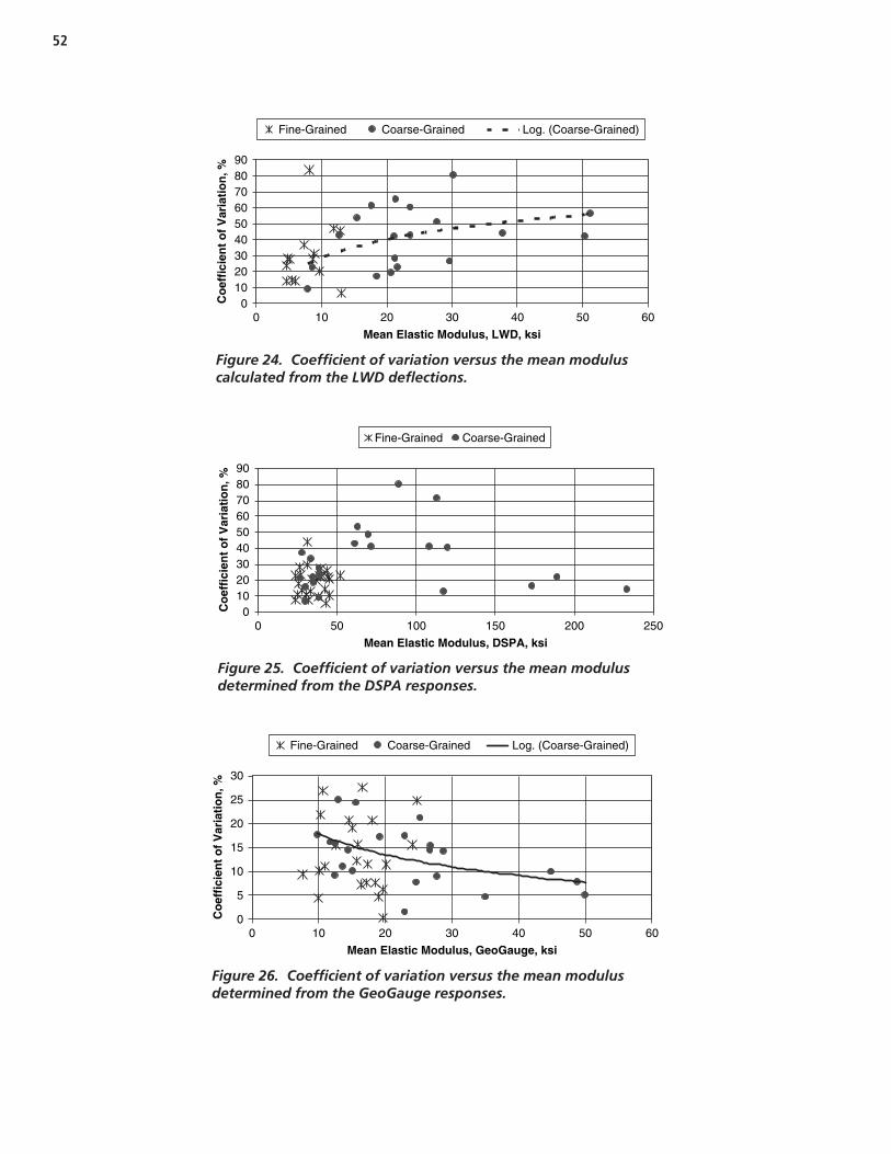
52
0 50 100 150 200 250
Mean Elastic Modulus, DSPA, ksi
0102030405060
8090
70
Co
effi
cien
t o
f V
aria
tio
n, %
Fine-Grained Coarse-Grained
Figure 25. Coefficient of variation versus the mean modulusdetermined from the DSPA responses.
Fine-Grained Coarse-Grained Log. (Coarse-Grained)
0
5
10
15
20
25
30
0 10 20 30 40 50 60
Mean Elastic Modulus, GeoGauge, ksi
Co
effi
cien
t o
f V
aria
tio
n, %
Figure 26. Coefficient of variation versus the mean modulusdetermined from the GeoGauge responses.
Fine-Grained Coarse-Grained Log. (Coarse-Grained)
0102030405060
8090
70
0 10 20 30 40 50 60
Mean Elastic Modulus, LWD, ksi
Co
effi
cien
t o
f V
aria
tio
n, %
Figure 24. Coefficient of variation versus the mean moduluscalculated from the LWD deflections.

53
10
20
30
40
50
60
0 4 82 6 10 12 14
Depth Below Surface, inches
Res
ilien
t M
od
ulu
sC
alcu
late
d f
rom
DC
PP
enet
rati
on
Rat
e, k
si
Ohio Crushed Stone North Dakota Crushed Stone
Florida Limerock Base
(a) Aggregate Base Materials/Layers.
0 4 82 6 10 12 14
Depth Below Surface, inches
0
5
10
15
20
25
Res
ilien
t M
od
ulu
sC
alcu
late
d f
rom
DC
PP
enet
rati
on
Rat
e, k
si
Oklahoma High PI Clay North Dakota Embankment
(b) Subgrade and Embankment Materials/Layers.
Figure 27. Modulus gradients in unbound layers, as determined with the DCP.
Where:ER = Resilient modulus, MPa.
DPI = Penetration rate or index, mm/blow.
The DSPA was also placed in different directions relative tothe roller direction for measuring modulus; the other NDTdevices do not have this capability—only an equivalent oraverage modulus value is reported for all directions. Figure 28compares the difference between the modulus values paralleland perpendicular to the roller’s direction to the modulusmeasured parallel to roller direction. For less stiff materials(especially fine-grained materials), there is no differencebetween the two readings. For stiffer, coarse-grained materials,however, there is a slight bias. The moduli measured parallelto roller direction were slightly higher, on the average. Thisdifference and bias resulted in a higher COV for the clusteredmeasurements.
EDPI
R = ⎛⎝⎜
⎞⎠⎟17 6
2921 12
0 64
.( ) .
.
(16)The LWD had higher variability in test results and
lower success rates. The higher COV value is related to the variability in the underlying layers and their influence onthe measured response with the deflection measuringdevices, as well as thickness variations of the layer beingevaluated. A constant layer thickness and subsurface con-dition were used.
The variability of the GPR and EDG for measuring the vol-umetric properties (density and fluids content) was found tobe significantly different from each other, as well as from theagencies’ QA data, when available. Both of these devices hadvery poor success rates in identifying physical differencesbetween different sections. The EDG resulted in very lowvariability in its estimates of dry density and water contentwithin a specific area or test section. Most of the COV valuesfor both properties were less than 2 percent (see Tables 27 and28). Thus, the average values determined at a test point andwithin a test section did not deviate significantly from theproject average that was determined from nuclear densitygauges and/or sand-cone tests.

54
Conversely, the GPR resulted in high variability of thedielectric values (see Table 29), as well as for the dry densities.The dry densities determined in some areas exceeded 160 pcf(see Figure 29)—an unlikely value. The reason for the improb-ably high as well as low values within a project was the assump-
tion used to convert the dielectric values to dry densities—aconstant water content for all areas within a lot was assumed.As a result, the GPR data interpretation technique needs to beimproved to determine the dry density and water contentalong the project prior to day-to-day use in QA programs.
Project Identification Area A B C DMean, pcf 107.92 108.9 108.6 107.7 I-85 Embankment, Silty Clay;
Section 1, Before IC Rolling COV, % 1.3 0.5 1.1 1.7 Mean, pcf 107.2 107.5 108.9 107.2 I-85 Embankment, Silty Clay;
Section 2, Before IC Rolling COV, % 0.8 0.8 1.1 1.9 Mean, pcf 108.1 108.2 108.5 108.4 I-85 Embankment, Silty Clay;
Section 1, After IC Rolling COV, % 1.0 0.5 0.7 0.3 Mean, pcf 107.4 107.7 108.0 107.6 I-85 Embankment, Silty Clay;
Section 2, After IC Rolling COV, % 0.5 0.5 0.8 1.3 Mean, pcf 123.9 123.7 124.4 --- TH-23 Embankment, Silt-Sand-
Gravel Mix; North Section COV, % 0.4 0.1 1.0 --- Mean, pcf 122.5 122.9 122.9 ---TH-23 Embankment, Silt-Sand-
Gravel Mix; South Section COV, % 1.8 1.8 0.8 ---Mean, pcf 123.7 123.7 124.9 --- SH-130 Improved
Embankment; Section 1 COV, % 0.3 0.1 0.6 --- Mean, pcf 122.6 123.1 122.7 --- SH-130 Improved
Embankment; Section 2 COV, % 2.0 2.0 0.8 --- Mean, pcf 123.3 122.3 123.7 SH-130 Improved
Embankment; Section 3 COV, % 1.4 0.1 0.2 Mean, pcf 129.9 129.8 129.8 --- TH-23 Crushed Aggregate;
North Section COV, % 0 0 0 --- Mean, pcf 129.8 129.8 129.8 ---TH-23 Crushed Aggregate;
Middle Section COV, % 0 0 0 ---Mean, pcf 129.8 129.9 129.8 --- TH-23 Crushed Aggregate;
South Section COV, % 0.1 0.1 0 --- Mean, pcf 147.4 US-280 Crushed Stone; Section
1 COV, % 0.7 Mean, pcf 148.8 US-280 Crushed Stone; Section
2 COV, % 0.3 Mean, pcf 145.9 US-280 Crushed Stone; Section
3 COV, % 0.5 Mean, pcf 148.2US-280 Crushed Stone; Section
4 COV, % 0.3Note: The shaded cells designate those areas with anomalies (refer to Table 14); the black cells denote the weaker areas, while the gray cells denote the stronger areas tested within a specific project.
Table 27. Dry densities measured with the EDG, pcf.
-40-30-20-10
010203040
0 10 20 30 40 50 60 70 80
Adjusted Seismic Modulus Parallel to Roller Direction,DSPA, ksi
Res
idu
al (
E, P
aral
lel -
E,
Per
pen
dic
ula
r), k
si
Coarse-Grained Fine-Grained Zero Residual Line
Figure 28. DSPA modulus values measured parallel to rollerdirection versus the difference between modulus values parallel and perpendicular to roller direction.

55
2.3.1.2 Standard Error
Another reason for using the adjustment ratios in evaluat-ing each NDT device is to eliminate or reduce bias by assum-ing that the target value is the laboratory resilient modulusmeasured at a specific stress state. Figure 30 compares the lab-oratory measured resilient modulus values to those estimatedwith different NDT devices but adjusted to laboratory con-ditions, while Figure 31 presents the residuals (laboratoryresilient modulus minus the NDT modulus), assuming thatthe laboratory value is the target value. On the average, theadjusted elastic modulus from all devices compare reasonablywell with the laboratory measured resilient modulus. Table 30contains the tabulation of the mean of the residuals and stan-dard error for the NDT devices that provide a direct measureof material stiffness.
In summary, the GeoGauge, DSPA, and DCP all providegood estimates with negligible bias (effect of adjustmentratios) of the laboratory measured resilient modulus val-ues. The GeoGauge has the lower standard error. The LWDhas a higher bias and over two times the standard error, incomparison to the GeoGauge.
2.3.2 NDT Devices for HMA Mixtures
2.3.2.1 Variability of Response Measurements
Figure 32 compares the COV between different tech-nologies and devices (PSPA, FWD, PQI, and GPR). ThePQI consistently had a low COV relative to the otherdevices, while the FWD had the largest value. It should benoted that a low COV does not necessarily mean that thedevice is providing an accurate measure of the HMA mix-ture property and variability. One reason for the lowerCOV values for the PQI relative to the other devices is thatfive tests were performed at each test point. In other words,the testing and sampling error or differences get averagedout through the testing sequence.
Two versions of the GPR air-coupled antennas were used.The first version was a single-antenna method, which wasonly used in Part A of the field evaluation. The second versionincluded the use of multiple antennas and the EPIC HyperOptics™ proprietary data interpretation system. The EPICGPR system was supposed to be used along the NCAT, Mis-souri (US-47), and Texas (I-20) sections; however, weather
Project Identification Area A B C DMean, % 16.9 16.8 16.9 16.9 I-85 Embankment, Silty Clay;
Section 1, Before IC Rolling COV, % 0.8 0.3 0.3 1.0 Mean, % 16.9 16.9 16.8 17.0 I-85 Embankment, Silty Clay;
Section 2; Before IC Rolling COV, % 0.7 0.3 0.3 1.5 Mean, % 16.9 16.9 16.9 16.9 I-85 Embankment, Silty Clay;
Section 1, After IC Rolling COV, % 0.5 0.3 0.4 0 Mean, % 17.0 16.9 16.9 16.9 I-85 Embankment, Silty Clay;
Section 2, After IC Rolling COV, % 0.5 0.3 0 0.7 Mean, % 8.0 8.0 7.6 TH-23 Embankment, Silt-Sand-
Gravel Mix; North Section COV, % 5.1 1.1 11.9 Mean, % 9.8 8.7 7.6TH-23 Embankment, Silt-Sand-
Gravel Mix; South Section COV, % 7.5 7.3 15.8Mean, % 8.1 8.05 7.23 SH-130 Improved
Embankment; Section 1 COV, % 4.4 1.2 6.8 Mean, % 8.85 8.43 8.7 SH-130 Improved
Embankment; Section 2 COV, % 19.8 21.6 8.4 Mean, % 8.35 9.1 8.05 SH-130 Improved
Embankment; Section 3 COV, % 14.4 1.6 0.9 Mean, % 4.26 4.28 4.34 TH-23 Crushed Aggregate;
North Section COV, % 1.3 1.0 2.1 Mean, % 4.24 4.28 4.30TH-23 Crushed Aggregate;
Middle Section COV, % 1.3 2.0 1.6Mean, % 4.18 4.18 4.38 TH-23 Crushed Aggregate;
South Section COV, % 3.9 3.9 1.0 Mean, % 3.92 US-280 Crushed Stone;
Section 1 COV, % 3.1 Mean, % 4.18 US-280 Crushed Stone;
Section 2 COV, % 2.9 Mean, % 3.77 US-280 Crushed Stone;
Section 3 COV, % 2.9 Mean, % 4.06US-280 Crushed Stone;
Section 4 COV, % 2.6Note: The shaded cells designate those areas with anomalies (refer to Table 14); the black cells denote weaker areas, while the gray cells denote the stronger areas tested within a specific project.
Table 28. Water content measured with the EDG, percent.

56
delays and equipment/plant problems resulted in changes tothe testing schedule. These schedule changes resulted in con-flicts with other projects, so ultimately, this system was usedonly on the NCAT test sections.
Data were made available for use from other projects inFlorida, which were not included in the original field evalu-ation (Greene 2007; Greene and Hammons 2006). The EPICsystem is reported to have much more accurate and repeat-able estimates of HMA volumetric properties. One reasonfor this increased accuracy and precision is that it does notrely on the assumptions that were included in the singleantenna method used along the Part A projects. The preci-sion and bias for both devices and systems are provided inthe next section.
2.3.2.2 Standard Error
As for the unbound materials, the adjustment ratios were used in evaluating the PSPA and FWD to reduce bias
by assuming that the target value is the laboratory dynamicmodulus measured at a specific load frequency and an aver-age in-place mix temperature. Figure 33 compares thePSPA and FWD modulus values that have been adjusted tolaboratory conditions using the factors or ratios listed inTable 26. On the average, the adjusted modulus valuescompare reasonably well to one another. Table 31 containsthe mean of the residuals (laboratory dynamic modulusminus the NDT modulus) and standard error from theexpected laboratory value—excluding all measurementstaken in areas with anomalies, segregation, and along lon-gitudinal joints.
While the difference between the two NDT devices is small,the PSPA had the lower residual and standard error.
2.3.3 Summary
Tables 32, 33, and 34 contain the statistical analyses of theNDT devices included in the field evaluation projects. This
Project Identification Area A B C DMean 15.38 15.79 14.29 15.19 I-85 Embankment, Silty Clay; Section
1, Before Rolling COV, % 17.8 23.3 53.6 25.7 Mean 13.91 17.47 16.82 16.38 I-85 Embankment, Silty Clay; Section
2, Before IC Rolling COV, % 29.0 20.5 30.7 24.1 Mean 20.37 21.23 21.61 23.23 I-85 Embankment, Silty Clay; Section
1, After IC Rolling COV, % 15.8 10.6 15.0 12.6 Mean 19.13 23.75 23.77 25.36 I-85 Embankment, Silty Clay; Section
2; After IC Rolling COV 10.2 10.7 17.6 8.4 Mean 23.004 13.468 19.334 ---TH-23 Embankment, Silt-Sand-
Gravel Mix; South Section COV, % 11.3 7.0 14.4 ---Mean 20.324 34.438 23.882 --- TH-23 Embankment, Silt-Sand-
Gravel Mix; North Section COV, % 22.2 32.7 22.7 --- Mean 9.225 10.00 7.65 --- SH-130 Improved Embankment;
Section 1 COV 33.1 42.3 42.9 --- Mean 12.875 8.875 9.825 --- SH-130 Improved Embankment;
Section 2 COV 90.3 47.4 20.1 Mean 8.775 9.025 11.85 SH-130 Improved Embankment;
Section 3 COV, % 51.5 50.8 48.7 --- Mean --- 8.796 10.042 --- TH-23 Crushed Aggregate; North
Section COV, % --- 1.6 5.4 --- Mean --- 8.950 10.87 ---TH-23 Crushed Aggregate; Middle
Section COV, % --- 6.1 10.9 ---Mean --- 9.792 10.378 --- TH-23 Crushed Aggregate; South
Section COV, % --- 8.2 4.3 --- Mean 11.723 US-280 Crushed Stone; Section 1
COV, % 8.3 Mean 12.222
US-280 Crushed Stone; Section 2 COV, % 11.4
Mean 11.919 US-280 Crushed Stone; Section 3
COV, % 7.3 Mean 11.569US-280 Crushed Stone; Section 4
COV, % 7.0Notes:
The shaded cells designate those areas with anomalies (refer to Table 14); the black cells denote the weaker areas, while the gray cells denote the stronger areas tested within a specific project.Due to construction sequencing, lane A of the TH-23 crushed aggregate base sections could not be tested with the GPR after it arrived on site.
Table 29. Dielectric values measured with the GPR on the unbound layers.

information is grouped into two areas—those NDT deviceswith an acceptable to excellent success rate and those withpoor success rates in identifying material/layer differences.
2.4 Comparison of Results BetweenNDT Technologies
This section provides a brief evaluation and comparison ofthe test results between different technologies to determinethe reasons for the low success rates of the DCP, LWD, GPR,and EDG.
2.4.1 NDT Modulus Comparisons
Figure 34 compares the NDT modulus values used toidentify areas with physical differences in the unbound lay-ers, except that the NDT values have been adjusted to lab-
oratory conditions with the adjustment ratios listed inTable 24. Figure 34(a) includes a comparison of the indi-vidual test points, while Figure 34(b) compares the data ona project basis. Figure 33 compared the adjusted PSPA andFWD modulus for the HMA layers using the adjustmentratios listed in Table 25.
The adjustment procedure reduced the bias between thedifferent devices, but not the dispersion. Thus, any of theseNDT modulus estimating devices can be used to estimate theresilient modulus of the material with proper calibration atthe beginning of the project, with some exceptions.
• Deflection-Based Devices: The calculated modulus valuesfrom the deflection-based devices can be affected greatly bythe underlying materials and soils. For example, the crushedstone base material placed in area 4 along US-280 nearOpelika, Alabama, is a stiff and dense material, even though
57
200.0 300.0 400.0 500.0 600.0110
120
130
140
150
160
170
Den
sity
(pc
f)
7956+00.4 7957+00 7958+00 7959+00 7959+99.4
1800.0 1900.0 2000.0 2100.0
Distance from S Catch Basin (ft.)
110
120
130
140
150
160
170
Dep
th (
in.)
GPS Stations
7971+23.3 7972+23.4 7973+22.3 7974+21.9 7975+21.9
Base Sections - Base Density
INFRASENSE, Inc.
TH23 - Spicer, MN
Arlington, MA 02476
Sheet: 1 of 1
Analyzed by: GLM Date: 10/21/04Checked by: KRM Date: 10/22/04
800.0 900.0 1000.0 1100.0 1200.0110
120
130
140
150
160
170
Den
sity
(pc
f)
7962+00.5 7963+02.1 7964+02.5 7965+04 7966+04.2
Moisture Content Assumed Constant at 4.12%
Figure 29. Density profiles generated from the GPR test results for the crushed aggregate base layerplaced along the TH-23 reconstruction project.

58
Geo., Fine-Grained Geo., Coarse-Grained Line of Equality
DSPA, Fine-Grained DSPA, Coarse-Grained
(b) Deflection-Based and DCP methods.
0
10
20
30
40
50
60
Ad
just
ed E
last
ic M
od
ulu
sfr
om
ND
T D
evic
es, k
si
0 10 20 30 40 50 60
Laboratory Resilient Modulus, ksi
(a) DSPA and the GeoGauge.
0 10 20 30 40 50 60
Laboratory Resilient Modulus, ksi
0
10
20
30
40
50
60
Ad
just
ed E
last
ic M
od
ulu
sfr
om
ND
T D
evic
es, k
si
DCP, Fine-Grained DCP, Coarse-Grained Line of Equality
LWD, Fine-Grained LWD, Coarse-Grained
Figure 30. Laboratory resilient modulus versus adjusted NDTmodulus.
-15
-10
-5
0
5
10
15
0 10 20 30 40 50 60
Laboratory Resilient Modulus,Target Value, ksi
Res
idu
al f
rom
Tar
get
Val
ue,
ksi
GeoGauge DSPA Zero Residual
(a) GeoGauge and DSPA.
-15
-10
-5
0
5
10
15
20
25
0 10 20 30 40 50 60
Laboratory Resilient Modulus, Target Value, ksi
Res
idu
al f
rom
Tar
get
Val
ue,
ksi
DCP LWD Zero Residual
(b) DCP and LWD.
Figure 31. Residuals (laboratory minus NDT modulus values) versus adjusted NDT modulus.

the deflection-based devices found it to be weaker than theother areas tested with a value less than 20 ksi. All otherNDT devices estimated the modulus for area 4 to be about35 ksi or higher. An in-place modulus of 20 ksi for thismaterial is too low. Thus, variations in the subsurface layersor materials/soils can incorrectly result in significant bias inthe resilient modulus.
• DSPA: The DSPA can significantly overestimate the labo-ratory measured resilient modulus values. The US-280crushed stone base was dry or significantly below the opti-mum water content during testing in some areas. It isbelieved that the surface of this dense, dry crushed stone isresponding like a bound layer—resulting in a much higher
modulus of the entire layer. In fact, the surface of thismaterial actually exhibited radial cracks during the seatingdrop of the DCP. Figure 35 shows the estimated moduluswith depth from the DCP.
2.4.2 NDT Volumetric Property Comparisons
2.4.2.1 Unbound Layers
The EDG and GPR were used to estimate the volumetricproperties of the unbound materials. The following list pro-vides a summary of the response measurements to the dry
59
NDT Device GeoGauge DSPA DCP LWDMean Residual, ksi -0.117 0.149 -0.078 0.614 Standard Error, ksi 2.419 4.486 3.768 5.884
Table 30. Tabulation of the mean of the residualsand standard error for NDT devices.
0
5
10
15
20
25
30
35
0 5 10 15 20 25 30 35
PSPA Coefficient of Variation, percent
Co
effi
cien
t o
f V
aria
tio
n,
Oth
er D
evic
es, p
erce
nt
FWD PQI GPR Line of Equality
Figure 32. Comparison of coefficients of variation of different NDT devices.
100
200
300
400
500
600
700
100 200 300 400 500 600 700
Adjusted Seismic Modulus, PSPA, ksi
Ad
just
ed E
last
ic M
od
ulu
s,F
WD
, ksi
Adjusted to Laboratory Conditions Line of Equality
Figure 33. Comparison of the PSPA and FWD modulus valuesadjusted to laboratory conditions.
NDT Device PSPA FWDMean Residual, ksi 13.5 39.0 Standard Error, ksi 76 87
Table 31. Tabulation of the mean of the residuals and standard error for NDT devices from the expected laboratory value.
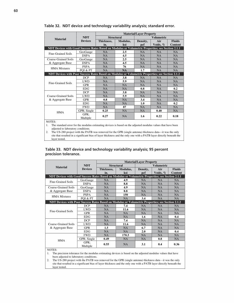
60
Material/Layer Property Structural VolumetricMaterial NDT
Devices Thickness,in.
Modulus,ksi
Density,pcf
AirVoids, %
FluidsContent
NDT Devices with Good Success Rates Based on Modulus or Volumetric Properties; see Section 2.1.1 GeoGauge NA 2.5 NA NA NA
Fine-Grained Soils DSPA NA 4.5 NA NA NA
GeoGauge NA 2.5 NA NA NACoarse-Grained Soils & Aggregate Base DSPA NA 4.5 NA NA NA
PSPA NA 76 NA NA NAHMA Mixtures
PQI & PT NA NA 1.7 NA NANDT Devices with Poor Success Rates Based on Modulus or Volumetric Properties; see Section 2.1.2
DCP NA 3.8 NA NA NALWD NA 5.9 NA NA NAGPR NA NA NA NA NA
Fine-Grained Soils
EDG NA NA 0.8 NA 0.2DCP NA 3.8 NA NA NALWD NA 5.9 NA NA NAGPR 0.8 NA 3.4 NA NA
Coarse-Grained Soils & Aggregate Base
EDG NA NA 1.0 NA 0.2FWD NA 87 NA NA NA
GPR; Single 0.25 NA NA 0.40 NAHMA GPR;
Multiple 0.27 NA 1.6 0.22 0.18
NOTES: 1. The standard error for the modulus estimating devices is based on the adjusted modulus values that have been
adjusted to laboratory conditions. 2. The US-280 project with the PATB was removed for the GPR (single antenna) thickness data—it was the only
site that resulted in a significant bias of layer thickness and the only one with a PATB layer directly beneath the layer tested.
Table 32. NDT device and technology variability analysis; standard error.
Material/Layer Property Structural VolumetricMaterial NDT
Devices Thickness,in.
Modulus,ksi
Density,pcf
AirVoids, %
FluidsContent
NDT Devices with Good Success Rates Based on Modulus or Volumetric Properties; see Section 2.1.1 GeoGauge NA 4.9 NA NA NA
Fine-Grained Soils DSPA NA 8.8 NA NA NA
GeoGauge NA 4.9 NA NA NACoarse-Grained Soils & Aggregate Base DSPA NA 8.8 NA NA NA
PSPA NA 150 NA NA NAHMA Mixtures
PQI & PT NA NA 3.4 NA NANDT Devices with Poor Success Rates Based on Modulus or Volumetric Properties; see Section 2.1.2
DCP NA 7.4 NA NA NALWD NA 11.6 NA NA NAGPR NA NA NA NA NA
Fine-Grained Soils
EDG NA NA 1.6 NA 0.4DCP NA 7.4 NA NA NALWD NA 11.6 NA NA NAGPR 1.5 NA 6.7 NA NA
Coarse-Grained Soils & Aggregate Base
EDG NA NA 2.0 NA 0.4FWD NA 170.5 NA NA NA
GPR; Single 0.49 NA NA 0.8 NAHMA GPR;
Multiple 0.55 NA 3.1 0.4 0.36
NOTES: 1. The precision tolerance for the modulus estimating devices is based on the adjusted modulus values that have
been adjusted to laboratory conditions. 2. The US-280 project with the PATB was removed for the GPR (single antenna) thickness data—it was the only
site that resulted in a significant bias of layer thickness and the only one with a PATB layer directly beneath the layer tested.
Table 33. NDT device and technology variability analysis; 95 percent precision tolerance.
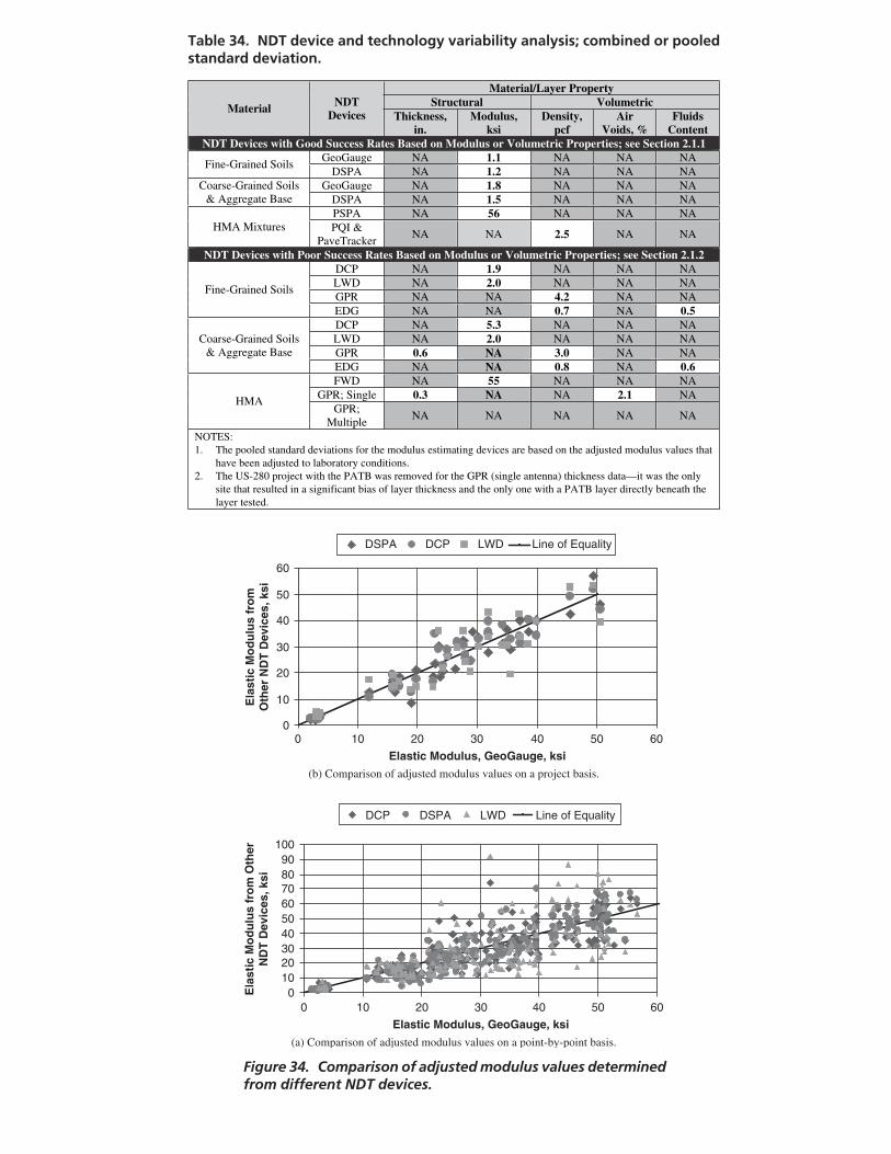
Material/Layer Property Structural VolumetricMaterial NDT
Devices Thickness,in.
Modulus,ksi
Density,pcf
AirVoids, %
FluidsContent
NDT Devices with Good Success Rates Based on Modulus or Volumetric Properties; see Section 2.1.1 GeoGauge NA 1.1 NA NA NA
Fine-Grained Soils DSPA NA 1.2 NA NA NA
GeoGauge NA 1.8 NA NA NACoarse-Grained Soils & Aggregate Base DSPA NA 1.5 NA NA NA
PSPA NA 56 NA NA NAHMA Mixtures PQI &
PaveTrackerNA NA 2.5 NA NA
NDT Devices with Poor Success Rates Based on Modulus or Volumetric Properties; see Section 2.1.2 DCP NA 1.9 NA NA NALWD NA 2.0 NA NA NAGPR NA NA 4.2 NA NA
Fine-Grained Soils
EDG NA NA 0.7 NA 0.5DCP NA 5.3 NA NA NALWD NA 2.0 NA NA NAGPR 0.6 NA 3.0 NA NA
Coarse-Grained Soils & Aggregate Base
EDG NA NA 0.8 NA 0.6FWD NA 55 NA NA NA
GPR; Single 0.3 NA NA 2.1 NAHMA GPR;
Multiple NA NA NA NA NA
NOTES: 1. The pooled standard deviations for the modulus estimating devices are based on the adjusted modulus values that
have been adjusted to laboratory conditions. 2. The US-280 project with the PATB was removed for the GPR (single antenna) thickness data—it was the only
site that resulted in a significant bias of layer thickness and the only one with a PATB layer directly beneath the layer tested.
Table 34. NDT device and technology variability analysis; combined or pooledstandard deviation.
0
10
20
30
40
50
60
0 10 20 30 40 50 60
Elastic Modulus, GeoGauge, ksi
Ela
stic
Mo
du
lus
fro
mO
ther
ND
T D
evic
es, k
si
DSPA DCP LWD Line of Equality
(b) Comparison of adjusted modulus values on a project basis.
0102030405060708090
100
0 10 20 30 40 50 60
Elastic Modulus, GeoGauge, ksi
Ela
stic
Mo
du
lus
fro
m O
ther
ND
T D
evic
es, k
si
DCP DSPA LWD Line of Equality
(a) Comparison of adjusted modulus values on a point-by-point basis.
Figure 34. Comparison of adjusted modulus values determinedfrom different NDT devices.

62
0
10
20
30
40
50
60
0 42 6 8 10 12
Depth Below the Surface, inches
Res
ilien
t M
od
ulu
s E
stim
ated
fro
m t
he
DC
P P
enet
rati
on
Rat
e, k
si
US-280 Base; Area 1-C US-280; Area 1-A
Figure 35. Modulus gradient measured with the DCP for theUS-280 crushed stone base material.
0
10
20
30
40
50
100 110 120 130 140 150
Dry Density, EDG, pcf
Die
lect
ric
Val
ues
, GP
R
I-85 Embankment TH-23 Embankment SH-130 Subgrade
TH-23 Base US-280 Base
Figure 36. GPR dielectric values versus the EDG dry densitiesmeasured along different projects.
densities obtained from construction records and traditionalvolumetric tests.
• Figure 36 compares the dielectric values to the dry densitiesmeasured with the EDG. No good correlation was foundbetween the different materials tested. In addition, nodefined relationship was found between the two responsemeasurements for the same material. This observationsuggests that there are different properties affecting theEDG and GPR results—none of which could identify thephysical differences at a reasonable success rate.
• Figure 37 compares the GPR dielectric values to the drydensity measured with different devices—the EDG, nucleardensity gauges, and sand-cone tests. No good correlationwas found; only a trend was identified between the GPRresults and the densities obtained from construction records.As the dry density increased, the GPR dielectric values
decreased, but across significantly different materials.Changes in material density along the same project werepoorly correlated to changes in the dielectric value.
• Figure 38 compares the dry densities measured with theEDG to those measured with a traditional nuclear den-sity gauge. There are two definite groups of data—onefor fine-grained soils and the other for crushed aggregatebase materials. As the dry density increased between dif-ferent materials, the density from the EDG also increased.Within each group, however, no reasonable relationshipwas found.
2.4.2.2 HMA Layers
Figure 39 compares the air voids measured with the GPR tothe results from other devices and methods. Figure 39(a) com-pares the densities measured directly with the nuclear density

63
90
100
110
120
130
140
150
0 10 20 30 40 50
GPR Dielectric Values
Dry
Den
sity
, pcf
Electrical Density Gauge Nuclear Density Gauge
Power (Nuclear Density Gauge)
Figure 37. GPR dielectric values versus dry densities measuredwith nuclear and non-nuclear density gauges.
9095
100105110115120125130135140
90 95 100 105 110 115 120 125 130 140135
Dry Density, EDG, pcf
Dry
Den
sity
, Nuc
lear
Den
sity
Gau
ge
Series1 Line of Equality
Figure 38. Dry densities measured with the EDG and nuclear density gauges.
gauge and PQI. There is a general trend between the air voidmeasurements and densities—as air voids increase, the densitydecreases, but any correlation is poor. There are significant dif-ferences between the volumetric properties measured withthese different devices. Figure 39(b) compares the air voids cal-culated from the maximum theoretical density provided foreach mixture to the air voids estimated from the GPR dielec-tric values. As shown, no correlation exists between the devicesfrom the field evaluation projects included in this study.
Figure 40 compares the densities measured with thenuclear density gauge and the PQI along the longitudinaljoints and in areas with localized segregation. These densitiesare compared with the values measured away from the jointsand outside any noticeable segregation. There is a greatervariation in density measured with the nuclear device thanwith the PQI. However, the wet surface may have affected thePQI readings when the measurements were recorded.
2.4.3 Volumetric—Modulus Comparisons
2.4.3.1 Unbound Layers
The in-place modulus of the unbound materials is depen-dent on its density. The FHWA-LTPP study reported that thelaboratory resilient modulus was dependent on dry densityfor all unbound materials (Yau and Von Quintus). In fact,density and water content are two volumetric properties thathave a significant affect on the modulus of the material. Thus,it follows that the NDT devices resulting in a material modu-lus should be related to the density and/or water content ofthe material. Dry densities and water contents were extractedfrom the QA reports for the different projects included in thefield evaluation.
Figure 41 compares the average modulus values esti-mated from the different NDT devices and dry densitiesreported by the individual agencies during construction.

64
120
130
140
150
160
170
120 140 160130 150 170
Density, nuclear, pcf
Den
sity
, PQ
I, p
cf
Joint Readings Segregated Areas HMA Mixture Line of Equality
Figure 40. Nuclear density gauge measurements compared to the PQI values along longitudinal joints and in areas with segregation.
130
140
150
160
170
4 6 8 10 12 14 16
Air Voids, GPR, percent
Den
sity
, pcf
PQI - TH-23 Base PQI - SMA Overlay PQI - US-280 Base
PQI - US-280 Base Nuclear - SMA Overlay Nuclear - US-280 Base
(a) Density measured with the different devices.
0
2
4
6
8
10
12
14
0 2 4 6 8 10 12 14
Air Voids, GPR, percent
Air
Vo
ids,
Oth
er D
evic
es,
per
cen
t
PQI, TH-23 PQI, SMA Nuclear, SMA PQI, US-280
Nuclear, US-280 PQI, US-280 Line of Equality
(b) Air voids calculated from the maximum theoretical density for the mixture.
Figure 39. Air voids measured with the GPR versus densitiesmeasured with the PQI and nuclear density gauges for different HMA mixtures.

65
(a) Unadjusted modulus values.
0
10
20
30
40
50
60
Mo
du
lus
fro
m N
DT
Tes
ts,
Un
adju
sted
, ksi
GeoGauge DCP LWD Poly. (DCP) Poly. (GeoGauge)
100 110 120 130 140 150 160
Dry Density, QA Records, pcf
0
10
20
30
40
50
60
100 110 120 130 140 150 160
Dry Density, QA Records, pcf
Ad
just
ed M
od
ulu
s fr
om
ND
T T
ests
, ksi
GeoGauge DCP LWD
DSPA Poly. (GeoGauge) Poly. (DCP)
(b) Modulus values adjusted to laboratory conditions.
Figure 41. Dry density versus NDT adjusted modulus valuesfor different materials.
The important observation from this comparison is thatthere is a good relationship between dry density and theDCP estimated modulus, prior to adjusting the modulusvalues to laboratory conditions (Figure 41[a]). The resilientmodulus from the GeoGauge is also related to the dry den-sity of the material, but appears to become insensitive todry density for less dense, fine-grained soils with high watercontent. The resilient modulus from the LWD is related todry density but has the greatest variation because of theinfluence of the underlying materials.
Figure 41(b) graphically presents the same comparisonincluded in Figure 40(a), but using the adjusted modulusvalues. The GeoGauge and DSPA have similar relationshipsto dry density for both conditions. The relationship for theDCP becomes less defined and it is improved for the LWD.Overall, the modulus values resulting from each NDT deviceare related to the dry density across a wide range material.The GeoGauge has the better correlation to dry density usingthe adjusted values, followed by the DSPA and DCP. Thus, theGeoGauge was the primary device used in comparing theelastic modulus to the EDG and GPR results.
The dry density and water contents from the QA recordswere fairly dispersed and were not taken at each NDT testlocation or individual area. As such, the QA data can only beused to evaluate the results for different types of materials,rather than actual density variations within a project or lot.The EDG was used to measure the density and water contentat specific test locations for the other NDT devices.
Figure 42 compares the dry densities measured with theEDG and modulus values estimated from the GeoGauge andDCP. The NDT modulus increases with increasing dry densityover a wide range of material types, which is consistent withprevious experience. However, there are clusters of data forthe EDG that correspond to similar unbound materials thatwere tested. Within each data cluster, the correspondencebetween dry density and NDT modulus is poor for bothdevices.
This observation suggests that there are other factors thatimpact the modulus within a specific area; for example,water content and amount of coarse aggregate varyingwithin each data cluster. The EDG did not measure largevariations in water content within each area. In summary,

66
the within-project area variation of the modulus valuesappears to be more dependent on properties other than drydensity (e.g., water content, gradation)—assuming that theEDG is providing an accurate estimate of the in-place drydensity. That assumption is questionable based on the dataaccumulated to date.
Figure 43 compares the GeoGauge modulus to the GPRdielectric values. No clear correspondence was found betweenthe dielectric values and modulus values. Specifically, a widerange of dielectric values and moduli were measured, but noconsistent relationship was found between the two properties.Thus, material/layer properties that affect modulus within anarea have little effect on the dielectric values.
2.4.3.2 HMA Layers
Figure 44 compares the PSPA modulus and the GPR airvoids. There is a general trend within this data set—decreasing
air voids and increasing PSPA modulus, but no good corre-lation. All NDT devices did correctly identify the differencebetween the US-280 initial and supplemental sections, withthe exception of the PQI. This difference was not planned butwas confirmed through the use of laboratory dynamic mod-ulus tests. The state agency’s and contractor’s QA data didnot identify any difference between these two areas or timeperiods.
Figure 45 compares the PSPA modulus and the PQI den-sity. A general trend exists for a specific mixture, but no cor-relation exists between these devices that can be used inday-to-day construction operations for control or accept-ance. A more important observation is that the volumetricmeasuring devices are not being influenced by those proper-ties that affect the modulus measuring NDT devices. As anexample, changes in the asphalt content and gradation inrelation to density, air voids, and stiffness changes do notaffect density measurements as they do modulus measure-
0
10
20
30
40
50
60
70
80
100 110 120 130 140 150 160
Dry Density, EDG, pcf
Ad
just
ed E
last
ic M
od
ulu
s, k
si
GeoGauge DCP Poly. (DCP)
Figure 42. NDT modulus values versus dry density measuredby the EDG.
0
10
20
30
40
50
60
0 10 20 30 40 50
GPR Dielectric Values
Res
ilien
t M
od
ulu
s, G
eoG
aug
e,ks
i
Figure 43. GPR dielectric values versus the GeoGauge modulus.

ments. This finding is applicable to all the NDT devices usedto test the HMA mixtures.
2.5 Supplemental Comparisons
This section provides an overview of three areas of supple-mentary information and data that were collected duringthe Part B field evaluation projects: (1) modulus and densitygrowth relationships for monitoring the rolling operations,(2) multiple operators and NDT devices, and (3) agency andcontractor use of NDT devices.
2.5.1 Modulus and Density-GrowthRelationships for Monitoring the Rolling Operation
Instrumented rollers were used on projects to monitor theincrease in density and stiffness of the unbound and HMAlayers, where the rollers could be scheduled for use. In acouple of cases, Asphalt Manager was on the project site, butit exhibited hardware or software problems. In other cases,
the unbound base layer had already been compacted by thecontractor, and the instrumented roller was only used to testthe surface. The contractor did not want to take the risk ofpotentially disturbing the aggregate base, requiring it to be re-compacted and tested. Figures 46 through 48 present some ofthe IC roller data, as related to HMA densities measured withother devices. Overall, the densities and stiffness measuredwith other devices correlated well with the output from theinstrumented rollers in the areas without localized anomalies.The instrumented rollers did not identify differences causedby localized anomalies (i.e., anomalies significantly less thanthe width of the roller).
Different NDT devices were also used to monitor thecompaction operation of HMA and unbound layers todemonstrate the value of these devices in real time. ThePSPA, DSPA, GeoGauge, and PaveTracker devices were usedon some of the Part A and most of the Part B field evaluationprojects. The following subsection contains importantobservations from the use of selected NDT devices for con-trolling the placement and compaction of both unboundand HMA layers in real time.
67
130
135
140
145
150
155
160
165
100 300 500200 400 600 700
PSPA Seismic Modulus, ksi
PQ
I Den
sity
, pcf
TH-23 Base SMA Overlay US-280 Base, InitialUS-280 Base, Supp.
Figure 45. PSPA modulus versus PQI density of HMA mixtures.
0
2
4
6
8
10
12
14
16
100 300200 400 500 600 700
PSPA Seismic Modulus, ksi
GP
R A
ir V
oid
s, p
erce
nt
TH-23 Base SMA Overlay US-280 Base, InitialUS-280 Base, Supp.
Figure 44. PSPA modulus versus GPR air voids.

2.5.1.1 Unbound Materials and Layers
Overall, the GeoGauge, DCP, and DSPA were successful inmonitoring the build up of modulus with the number ofroller passes for the unbound materials placed within the fieldevaluation, and they were beneficial in assisting the contractorin making decisions on the compaction operation used alongthe project. Some examples follow.
• Figure 49 presents data collected on a caliche base materialplaced along an entrance roadway from County Road 103near Pecos, Texas. Both the GeoGauge and DCP were used
to determine the increase in material modulus with com-paction. The DCP was used along this project because it wason a private facility, and delaying the compaction of this basematerial was not an issue. Both devices found an increase inmodulus with an increasing number of roller passes.
• Figure 50 presents data collected during the compaction ofa Missouri crushed limestone base material. The first rollerpass within this figure is after the material had been pre-liminarily compacted from other construction equipmentand roller passes. The maximum modulus for this materialwas achieved at about eight passes of the roller over a spe-cific area. The number of passes obviously is dependent on
68
U.S. 280 19.0 mm NMAS
y = 0.0819x + 131.94R2 = 0.47
130
135
140
145
150
155
160
0 50 150 250200100 300
Evib * 100, psi
Nu
clea
r D
ensi
ty, l
b/f
t^3
Figure 46. Comparison of the nuclear density gauge readings to theEvib values measured with the IC roller.
U.S. 280 19.0 mm NMAS
y = 0.0328x + 134.31R2 = 0.24
120
125
130
135
140
145
150
0 50 150 250200100 300
Evib * 100, psi
PQ
I Den
sity
, lb
/ft^
3
Figure 47. Comparison of the PQI density readings to the Evib valuesmeasured with the IC roller.

69
Location 3
130
135
140
145
150
155
160
0 1 2 3 4 4.53.52.51.50.5
Roller Passes
Den
sity
, lb/
ft^3
0
50
100
150
200
250
300
Density Site 6 Density Site 7 Evib Site 6 Evib Site 7
Figure 48. Example of a density growth curve prepared from the IC roller demonstration and NDT results.
5
10
15
20
25
30
0 42 6 8 10 12
Number of Roller Passes
Res
ilien
t M
od
ulu
s fr
om
ND
T D
evic
es, k
si
DCP GeoGauge Log. (GeoGauge) Log. (DCP)
Figure 49. Modulus-growth relationships for a calichebase along an entrance roadway to a facility fromCounty Road 103 near Pecos, Texas.
the water content of the in-place material; for the Missouricrushed limestone, the in-place water content was justbelow the optimum value.
• Figure 51 presents data collected during the compactionof a South Carolina crushed granite base material. Thiscrushed granite base material was difficult to compact withthe roller on the project site when compaction was initi-ated. In addition, the water content of this base materialwas well below the optimum value. Both the DSPA and theGeoGauge modulus values did not increase with the num-ber of roller passes. A nuclear density gauge was also usedalong the project, and it also showed no increase in densitywith the number of roller passes. Thus, rather than wasteadditional compaction effort, the contractor had to usea heavier roller and had to increase the water content ofthe material to obtain the specified density. This example
shows the benefit and advantage of using the GeoGauge orDSPA to make decisions in real time.
These examples show the benefit of developing modulus-growth curves using the DSPA or GeoGauge during con-struction for monitoring and optimizing the rolling pattern.
2.5.1.2 HMA Mixtures and Layers
Overall, the PSPA and PaveTracker were successful inmonitoring the build up of modulus and density with thenumber of roller passes for the HMA layers placed within thefield evaluation projects. Some examples follow.
• Figure 52 presents data collected along the Missouri widen-ing project (US-47) for two different areas. Figure 52(a)compares the densities measured using the contractor’snuclear density gauge on site for QC to those values mea-sured with the PaveTracker. The densities from the nucleargauge were related to the non-nuclear density gauge valueswith mixture specific calibration values. The contractorwas using one-test point readings with the nuclear gauge,while four readings at a test point were made with thePaveTracker within the same time.
The contractor was using the cold-side pinch methodfor compacting the longitudinal joint adjacent to the oldpavement. This HMA was tender based on visual observa-tions of its behavior under the roller—shoving of the matwas observed in front of, as well as across, the roller’sdirection. Rollers marks were also present after the lastpass of the finish roller. The HMA was being pushed away

10121416182022242628
0 2 4 6 81 3 5 7 9 10 11 12
Number of Roller PassesG
eoG
aug
e M
od
ulu
s, k
si
Missouri Crushed Limestone Base
0102030405060708090
0 42 6 8 10 12
Number of Roller Passes
DS
PA
Mo
du
lus,
ksi
0
5
10
15
20
25
30
Geo
Gau
ge
Mo
du
lus,
ksi
DSPA Modulus GeoGauge Modulus
Figure 50. Modulus-growth relationships for a Missouricrushed limestone base material for two different areas.
40
45
50
55
60
65
70
0 1 2 3 4 5 6 7 8 9 10 11 12 13 14 15 16 17
Number of Roller Passes
DS
PA
Mo
du
lus,
ksi
6
7
8
9
10
11
DSPA Modulus GeoGauge Modulus
5
6
7
8
9
10
0 4 2 6 8 10 12 14
Number of Roller Passes
Geo
Gau
ge
Mo
du
lus,
ksi
South Carolina Crushed Granite
Figure 51. Modulus-growth relationships for a South Car-olina crushed granite base material for two different areas.
70

from the confined longitudinal joint, rather than beingpushed down into the joint. Joint densities were madewith both the nuclear and non-nuclear density gaugesalong the joint, and the densities were found to be verylow—about 5 to 10 pcf below the densities measuredwithin the center of the mat. The contractor was asked tochange the rolling pattern for the confined longitudinaljoint using the hot-side method. With this method, thefirst pass of the roller is along the confined longitudinaljoint, with about a 6-in. overhang off the hot mat. Densi-ties were measured with both devices after changing therolling pattern. Figure 52(b) shows the densities along thelongitudinal joint, as compared to those in the center ofthe mat. The densities significantly increased after elimi-nating the roller pass on the cold side of the joint. Thus,the contractor was able to use the non-nuclear densitygauge in real time to significantly increase the joint den-sity by slightly revising the rolling pattern of the joint.
The PSPA was also used along this project, but the resultswere erratic during or immediately after compaction ofthe mat—the wave form was not consistent with HMAmixtures. The mixture was found to be too tender to obtainreliable readings, until the mix cooled below about 150°F.This HMA mixture was being used as the base for theshoulder or in a non-critical area. It was initially believedthat the PSPA had been damaged in transport, but thatwas found to be incorrect from latter testing of the HMAafter it had cooled down. At lower temperatures, the PSPAprovided reasonable results. Thus, its use would have beena benefit in identifying a tender mix, if this mix had beenused in a critical area under heavy traffic. Attempts weremade to use the PSPA on a couple of other projects, but thetemperature of those mixtures was too high to obtain reli-able results. Mix temperature is a limitation on testingHMA mixtures during rolling.
• Figure 53 presents density data collected on a MissouriHMA base mixture that was not tender, but was rolledwithin the temperature sensitive zone. The first pass of therubber-tired roller increased the density, but additionalpasses of that roller significantly decreased the density ofthe mat. The nuclear density gauge being used on site forQC gave the same results. The nuclear gauge, however, wasnot being used after each roller pass. This mixture did notexhibit the traditional mix “checking” or tearing under therollers, but the non-nuclear density gauge did identify thedetrimental effect of rolling within the temperature sensi-tive zone. More roller passes were required to regain thedensity that was lost by rolling within the temperature sen-sitive zone. Many of the other HMA mixtures that wereincluded within the field evaluation projects also exhibited
this temperature sensitivity under the rollers. SelectingHMA mixtures that checked and tore for the field evalua-tion was not planned.
• The I-75 Michigan overlay project was another projectwhere a HMA mixture was rolled within its temperaturesensitive zone. With three passes of a SAKAI vibratoryroller in the primary roller position, the HMA mixturedensity was greater than the specified value (see Figure 54).However, an intermediate roller continued to roll the mix,and was followed by two additional rollers. The use of thePaveTracker determined that the contractor was rollingin the temperature sensitive zone—the density began todecrease. By monitoring the density of the mat duringrolling, the result was that the contractor could eliminatetwo of the rollers and use fewer passes to obtain the requireddensity, as long as the rollers stayed out of the temperaturesensitive zone.
• Figure 55 shows an example for polymer modified asphalt(PMA) and conventional neat asphalt mixtures. These mix-tures were placed during the same time period. The conven-tional neat asphalt mixture exhibited the traditional checkingand tearing of the mat when it was rolled within the temper-ature sensitive zone, while the PMA mixture did not exhibittearing or checking. After pass 3 for the neat asphalt mix andafter pass 5 for the PMA mix, the densities decreased. Themix tearing and checking was observed under the roller toconfirm that the mix was rolled within the temperature zone.Thus, the mat had to be rolled much more to increase den-sity to the specified value for both mixtures.
Similar to the benefit for unbound layers, the non-nucleardensity gauges provide significant benefit to a contractor tooptimize the rolling pattern within the center of the mat, aswell as along longitudinal joints. The non-nuclear gauges canalso be used to determine when the rollers are being operatedwithin the temperature sensitive zone, so a contractor doesnot waste compaction effort or time and does not tear ordamage the HMA mix by operating the rollers within thetemperature sensitive zone.
2.5.2 Multiple Operators and NDT Gauges
For most of the Part B projects, multiple GeoGauges andPaveTrackers were used by different operators to determine theeffects of multiple operators on the variability of the devices.Figure 56 compares the measured responses from the twoGeoGauges that were used for testing unbound materials,while Figure 57 compares the measured densities from the twoPaveTracker devices used to monitor HMA mixtures. At theend of the field evaluation testing for each project, one of each
71

72
140141142143144145146147148149150
0 4 82 6 10 12 14 16
Number of Roller Passes
Den
sity
Mea
sure
d w
ith
Pav
eTra
cker
, pcf
Missouri HMA Mixture Compaction Operation:Pass 1-2; Vibratory RollerPass 3-4; Static Steel WheelPass 5-6; Vibratory RollerPass 7-11; Rubber TiredPass 12-14; Finish Roller
Figure 53. Density-growth relationship for an HMA base mixture from Missouri.
(a) PaveTracker versus nuclear gauge density measurements.
(b) PaveTracker density measurements made along a confined joint and within the center of the mat.
145
147
149
151
153
155
157
159
161
163
165
0 2 41 3 5
Number of Roller Passes
Den
sity
Mea
sure
d w
ith
Pav
eTra
cker
, pcf
170
180
190
200
210
220
230
Tem
per
atu
re o
f M
ixtu
re, °°
F
Mat Density Joint Density Mat Temperature Joint Temperature
136
138
140142
144
146
148150
152
154
0 2 41 3 5
Number of Roller Passes
HM
A M
at D
ensi
ty, p
cf
0
50
100
150
200
250
Mat
Tem
per
atu
re, °°
F
PaveTracker Density Nuclear Gauge Density Temperature
Figure 52. Typical density-growth curve measured with PaveTracker and nuclear densitygauge for the Missouri US-47 project.

device was left with the agency and contractor personnel. Thefollowing are observations from this comparative testing.
• Use of different GeoGauges and operators resulted in somebias that was modulus dependent for some materials; morebias was exhibited for the higher modulus values or stiffermaterial. Material specific calibration or adjustment factorsshould be determined and used for each material tested(see Table 24). This material specific calibration with asufficient number of replicate tests should minimize thebias between the different gauges. The variability betweendifferent gauges, however, will still exist.
• Use of different PaveTrackers and operators resulted inalmost no bias between the two gauges, with the exceptionof dense or high specific gravity mixtures. Material specificadjustments should be determined for these devices foreach mixture tested. The mixture specific factors shouldminimize bias, but the variability between different gaugeswill still exist.
2.5.3 Agency and Contractor Use of NDT Devices
During Part B of the field evaluation, one of the multiplegauges being used on a project was left with agency andcontractor construction personnel for continued use on aday-to-day QA basis. Those NDT devices left with the con-struction personnel included the GeoGauge, PSPA, andPaveTracker. Data from this additional use were includedin the comparison of multiple operators and devices at spe-cific project sites. This information was used in the evalua-tion described in Chapter 3, in determining the parametersneeded to set up control and acceptance plans when usingthese NDT devices.
The projects where construction personnel continued touse the devices included Missouri, North Dakota, andTexas. The NDT devices were going to be left at the Michi-gan I-75 project, but issues with the HMA mixture resultedin the project being stopped for a short term, so the con-
73
146.0
148.0
150.0
152.0
154.0
156.0
158.0
0 42 6 8 10 12
Number of Passes of the Rollers
Den
sity
of
Mat
Mea
sure
d w
ith
Pav
eTra
cker
, pcf
200
210
220
230
240
250
260
Tem
per
atu
re o
fM
ixtu
re, °°
F
Density Temperature
142.0
144.0
146.0
148.0
150.0
152.0
154.0
0 42 6 8 10 12
Number of Roller Passes
Den
sity
of
Mat
Mea
sure
d w
ith
Pav
eTra
cker
, pcf
210
220
230
240
250
260
270
Tem
per
atu
re o
fM
ixtu
re, ° °
F
SAKAI Vibratory SAKAI Pneumatic & Other Rollers
Temperature
VibratoryBreakdown
Roller
Intermediate &Finish Rollers
Figure 54. Density-growth curves for the Michigan mixturemeasured with PaveTracker and effects of rolling within thetemperature sensitive zone; two different areas.

struction personnel did not actually use the devices. For theMissouri project, weather delays resulted in the contractormoving to a different project so the devices were not usedon the same project, as that included in the Part B fieldevaluation. The devices were used for more than 2 weeks onthe North Dakota and Texas projects. In actuality, the con-tractor had already been using the PaveTracker and PSPAon the Texas I-20 project. The PaveTracker was a part of thecontractor’s standard or day-to-day QC plan, while thePSPA had been used on a research basis.
2.6 Summary of Evaluations
In summary, the steady-state vibratory (GeoGauge) andseismic (DSPA) technologies are suggested for use in judgingthe quality of unbound layers, while the seismic (PSPA) andnon-nuclear density gauges (the PaveTracker was used inPart B) are suggested for use on HMA layers. The GPR is sug-gested for layer thickness acceptance, while the IC rollers aresuggested for use on a control basis for compacting unboundand HMA layers. The following sections provide some of thereasons for these determinations.
2.6.1 NDT Devices for Unbound Layers and Materials
• The DSPA and GeoGauge devices had the highest successrates for identifying an area with anomalies, rates of 86 and79 percent, respectively. The DCP and LWD identifiedabout two-thirds of the anomalies, while the GPR andEDG had unacceptable rates, below 50 percent.
• Three to five repeat measurements were made at each testpoint with the NDT devices, with the exception of the DCP.— The LWD exhibited low standard deviations that were
less dependent on material stiffness with a pooled stan-dard deviation less than 0.5 ksi. One reason for the lowvalues is that the moduli were less than for the otherdevices. The COV, however, was higher. It is expectedthat the supporting layers had an effect on the resultsby reducing the modulus.
— The GeoGauge had a standard deviation for repeatabil-ity measurements varying from 0.3 to 3.5 ksi and werematerial dependent.
— The DSPA had the lowest repeatability with a stan-dard deviation varying from 1.5 to 21.5 ksi. The rea-son for this higher variation in repeat readings is that
74
132
134
136
138
140
142
144
0 42 6 8 10
Number of Roller Passes
Den
sity
Mea
sure
d w
ith
Pav
eTra
cker
, pcf
Florida PMA Base Mix
132
134
136
138
140
142
144
0 2 4 6 8 10 12
Number of Roller Passes
Den
sity
Mea
sure
d w
ith
Pav
eTra
cker
, pcf
Florida Neat Base Mix
Compaction Operation:Pass 1-4; Vibratory RollerPass 5; Static Steel DrumPass 6-8; Vibratory RollerPass 9; Finish Roller
Compaction Operation:Pass 1-4; Static Steel DrumPass 5-7; Rubber Tired RollerPass 8-10; Finish Roller
(a) Conventional Neat HMAMixture
(b) PMA Mixture
Figure 55. Density-growth curves for two Florida mixtures measured withPaveTracker and effects of rolling within the temperature sensitive zone.

the DSPA sensor bar was rotated relative to the direc-tion of the roller, while the other devices were keptstationary or did not have the capability to detectanisotropic conditions. No significant difference wasfound relative to the direction of testing for fine-grained soils, but there was a slight bias for the stiffercoarse-grained materials.
— The EDG was highly repeatable with a standard deviationin density measurements less than 1 pcf, while the GPRhad poor repeatability—based on point measurements.
Triplicate runs of the GPR were made over the samearea or sublot. For comparison to the other NDT devices,the values measured at a specific point, as close as possi-ble, were used. Use of point specific values from succes-sive runs could be a reason for the lower repeatability,which were probably driver specific. One driver wasused for all testing with the GPR.
• The COV was used to compare the normalized dispersionmeasured with different NDT devices. The EDG consis-tently had the lowest COV with values less than 1 percent.
75
Comparison between GeoGauge B 24C and B 25C (All Part B test data)
y = 0.9025x + 1.6607
R2 = 0.7615
0
5
10
15
20
25
30
35
40
45
0 5 10 15 20 25 30 35 40 45
GeoGauge, B 24C; Modulus, ksi
Geo
Gau
ge, B
25C
; M
odul
us, k
siComparison of GeoGauge B 24C and B 25C (By Section)
15
16
17
18
19
20
21
22
23
24
25
26
27
28
15 16 17 18 19 20 21 22 23 24 25 26 27 28
GeoGauge, B 24C; Modulus, ksi
Geo
Gau
ge, B
25C
; M
odul
us, k
si
(a) Comparison on a point-by-point basis. (b) Comparison on a project basis.
Comparison between GeoGauge B 24C and B 25C (Modulus, ksi)
5
10
15
20
25
30
35
40
45
5 10 15 20 25 30 35 40 45
GeoGauge, B 24C; Modulus, ksi
Geo
Gau
ge, B
25C
; Mod
ulus
, ksi
ND US-2 Base
NCAT, Missouri N10, Base
NCAT, Oklahoma, N8&N9, Subgrade
OH, SR-53, Base
Linear (ND US-2 Base)
Linear (NCAT, Missouri N10, Base)
Linear (NCAT, Oklahoma, N8&N9, Subgrade)
Linear (OH,SR-53, Base)
(c) Comparison on a material basis.
Figure 56. Comparison of modulus measurement with two independent GeoGauges.

The GeoGauge had a value of 15 percent, followed by theDSPA, LWD, DCP, and GPR. The GPR and EDG aredependent on the accuracy of other tests in estimating vol-umetric properties (density and moisture contents). Anyerror in the calibration of these devices for the specificmaterial is directly reflected in the resulting values. Thiscould be a probable reason why the GPR and EDG devicesdid not consistently identify the areas with anomalies orphysical differences.
• Repeated load resilient modulus tests were performed inthe laboratory for characterizing and determining thetarget resilient modulus for each material. Adjustmentratios were determined based on uniform conditions.The overall average ratio for the GeoGauge for the stiffercoarse-grained materials was near unity (1.05). For the
fine-grained, less stiff soils, the ratio was about 0.5. Afteradjusting for laboratory conditions, all NDT devices thatestimate resilient modulus resulted in low residuals (labo-ratory resilient modulus minus the NDT elastic modulus).However, the GeoGauge and DCP resulted in the loweststandard error. The LWD had the highest residuals andstandard error.
• The DSPA and DCP measured responses represent thespecific material being tested. The DCP, however, can be significantly affected by the varying amounts of aggregateparticles in fine-grained soils and the size of the aggregatein coarse-grained soils. The GeoGauge measured responsesare minimally affected by the supporting materials, whilethe LWD can be significantly affected by the supportingmaterials and thickness of the layer being tested. Thickness
76
Comparison between PaveTracker 10232 and 10233 (All Density Data)
y = 1.1315x - 17.635R2 = 0.2007
110
120
130
140
150
160
170
110 120 130 140 150 160 170
PaveTracker 10232; Density, pcf
Pav
eTra
cker
102
33; D
ensi
ty, p
cf
Comparison of PaveTracker 10232 and 10233 (Average Density, pcf)
120
125
130
135
140
145
150
155
160
165
170
120 130 140 150 160 170
PaveTracker 10232; Density, pcf
Pav
eTra
cker
102
33; D
ensi
ty, p
cf
(a) Comparison on a point-by-point basis. (b) Comparison on a project basis.
Comparison between PaveTracker 10232 and 10233 (Density, pcf)
110
120
130
140
150
160
170
110 120 130 140 150 160 170
PaveTracker 10232; Density, pcf
Pav
eTra
cker
102
33; D
ensi
ty, p
cf
MI I-75 Surface MO US-47 Surface ND US-2 Surface
OH SR-53 Base OH SR-53 Surface
(c) Comparison on a material or mixture basis.
y = 0.9506x + 7.1232R2 = 0.9179
Figure 57. Comparison of the density measurements with two non-nuclear PaveTracker devices used within thePart B field evaluation.

deviations and variable supporting layers are reasons thatthe LWD had a low success rate in identifying areas withanomalies or physical differences.
• No good or reasonable correlation was found between theNDT devices that estimate modulus and those devices thatestimate volumetric properties.
• The instrumented rollers were used on too few projects fora detailed comparison to the other NDT devices. The rollerswere used to monitor the increase in density and stiffnesswith an increasing number of roller passes. One potentialdisadvantage with these rollers is that they may bridge local-ized soft areas. However, based on the results obtained,their ability of provide uniform compaction was verifiedand these rollers are believed to be worth future investmentin monitoring the compaction of unbound materials.
• The GPR resulted in reasonably accurate estimates to thethickness of aggregate base layers. None of the other NDTdevices had the capability or same accuracy to determinethe thickness of the unbound layer.
2.6.2 NDT Devices for HMA Mixtures and Layers
• The PSPA had the highest success rate for identifying anarea with anomalies, 93 percent. The PQI identified aboutthree-fourths of the anomalies, while the FWD and GPRidentified about one-half of those areas. The seismic andnon-nuclear gauges were the only technologies that consis-tently identified differences between the areas with andwithout segregation. These two technologies also consis-tently found differences between the longitudinal joint andinterior of the mat.
• The non-nuclear density gauges (PaveTracker) were ableto identify and measure the detrimental effect of rolling theHMA mat within the temperature sensitive zone. Thistechnology was beneficial on some of the Part B projectsfor optimizing the rolling pattern initially used by thecontractor.
• Three to four repeat measurements were made at each testpoint with the NDT devices.— The PSPA had a repeatability value, a median or pooled
standard deviation, of about 30 ksi for most mixtures,with the exception of the US-280 supplemental mix-ture, which was much higher.
— The FWD resulted in comparable value for the SMAmixture (55 ksi), but had a higher value for the US-280mixture (275 ksi).
— The non-nuclear density gauges had repeatability valuessimilar to nuclear density gauges, a value less than 1.5 pcf.
— The repeatability for the GPR device was found to begood and repeatable, with values of 0.5 percent for airvoids and 0.05 in. for thickness.
• The PSPA moduli were comparable to the dynamic modulimeasured in the laboratory on test specimens compactedto the in-place density at a loading frequency of 5 Hz andthe in-place mixture temperature, with the exception ofone mixture—the US-280 supplemental mixture. In fact,the overall average ratio or adjustment factor for the PSPAwas close to unity (1.1). This was not the case for the FWD.Without making any corrections for volumetric differ-ences to the laboratory dynamic modulus values, the stan-dard error for the PSPA was 76 ksi (laboratory valuesassumed to be the target values). The PSPA was used onHMA surfaces after compaction and the day followingplacement. The PSPA modulus values measured immedi-ately following compaction were found to be similar to thevalues 1 or 2 days after placement—making proper tem-perature corrections in accordance with the master curvesmeasured in the laboratory.
• A measure of the mixture density or air voids is required tojudge the acceptability of the modulus value from a dura-bility standpoint. The non-nuclear gauges were found tobe acceptable, assuming that the gauges had been properlycalibrated to the specific mixture—as for the PSPA.
• Use of the GPR single antenna method, even with mixturecalibration, requires assumptions on specific volumetricproperties that do vary along a project. As the mixtureproperties change, the dielectric values may or may not beaffected. Use of the proprietary GPR analysis method onother projects was found to be acceptable for the air void orrelative compaction method. This proprietary and multipleantenna system, however, was not used within Part A of thefield evaluation to determine its success rate in identifyinglocalized anomalies and physical differences between differ-ent areas. Both GPR systems were found to be very good formeasuring layer thickness along the roadway.
• Water can have a definite affect on the HMA density mea-sured with the non-nuclear density gauges (PQI). The man-ufacturer’s recommendation is to measure the densityimmediately after compaction, before allowing any trafficon the HMA surface. Within this project, the effect of waterwas observed on the PQI readings, as compared to dry sur-faces. The measured density of wet surfaces did increase,compared to dry surfaces. From the limited testing com-pleted with wet and dry surfaces, the PaveTracker was lessaffected by surface conditions. However, wet versus drysurfaces were not included in the field evaluation plan fordifferent devices. Based on the data collected within thefield evaluation, wet surfaces did result in a bias of the den-sity measurements with this technology.
• Another important condition is the effect of time and vary-ing water content on the properties of the HMA mixtureduring construction. There have been various studies com-pleted on using the PSPA to detect stripping and moisture
77

damage in HMA mixtures. For example, Hammons et al.(2005) used the PSPA (in combination with GPR) to locateareas with stripping along selected interstate highways inGeorgia. The testing completed within this study also sup-ports the use of the seismic-based technology to identifysuch anomalies.
• The instrumented rollers used to establish the increase instiffness with number of passes was correlated to theincreases in density, as measured by different devices.These rollers were used on too few projects to develop orconfirm any correlation between the NDT response andthe instrumented roller’s response. One issue that willneed to be addressed is the effect of decreasing temperatureon the stiffness of the mixture and how the IC roller per-ceives that increase in stiffness related to increases in den-sity of the mat. A potential disadvantage with these rollersis that they will bridge segregated areas and may not accu-rately identify cold spots in the HMA mat. However, basedon the results obtained, the ability to provide uniformcompaction was verified, and the rollers are believed to beworth future investments in monitoring the compaction ofHMA mixtures.
2.6.3 Limitations and Boundary Conditions
The following lists the limitations and boundary conditionsobserved during the field evaluation for the NDT devicessuggested for QA application on an immediate, effective, andpractical basis.
• All NDT devices suggested for QA application, with theexception of the GPR and IC rollers, are point-specific tests.Point-specific tests are considered a limitation because ofthe number of samples required to identify localized anom-alies that deviate from the population distribution.— Ultrasonic scanners are currently under development.
Relatively continuous measurements can be made withthis technology. These scanners are still considered to bein the research and development stage and are not readyfor immediate and practical use in a QA program.
— GPR technology to estimate the volumetric propertiesof HMA mixtures is available for use on a commercialbasis, but the proprietary system has only had limitedverification of its potential use in QA applications andvalidation of all volumetric properties determined withthe system.
— Similarly, the IC rollers take continuous measurementsof density or stiffness of the material being compacted.During the field evaluation, some of these rollers hadboth hardware and software problems. Thus, thesedevices were not considered immediately ready for usein a day-to-day QA program. The equipment, however,
has been improved and its reliability has increased. Thetechnology is suggested for use on a control basis butnot for acceptance.
• Ultrasonic technology (PSPA) for HMA layers and materi-als is suggested for use in control and acceptance plans.— Test temperature is the main boundary condition for
the use of the PSPA. Elevated temperatures during mixplacement can result in erratic response measurements.Thus, the gauge may not provide reliable responses formonitoring the compaction of HMA layers or fordetermining when the rollers are operating within thetemperature sensitive zone for the specific mixture.
— These gauges need to be calibrated to the specific mix-ture being tested. However, this technology can be usedin the laboratory to measure the seismic modulus on testspecimens during mixture design or verification prior tomeasuring the dynamic modulus in the laboratory.
— A limitation of this technology is that the results(material moduli) do not provide an indication on thedurability of the HMA mixture. Density or air void mea-surements are needed to define durability estimates.
— The DSPA for testing unbound layers is influenced bythe condition of the surface. High modulus values nearthe surface of the layer will increase the modulus esti-mated with the DSPA. Thus, the DSPA also needs to becalibrated to the specific material being evaluated.
• Steady-state vibratory technology (GeoGauge) for unboundlayers and materials is suggested for use in control andacceptance plans.— This technology or device should be used with caution
when testing fine-grained soils with high water con-tents. In addition, it should not be used to test well-graded, non-cohesive sands that are dry.
— The condition of the surface of the layer is importantand should be free of loose particles. A layer of moistsand should also be placed to fill the surface voids andensure that the gauge’s ring is in contact with about75 percent of the material’s surface. Placing this thinlayer of moist sand takes time and increases the timeneeded for testing.
— These gauges need to be calibrated to the specific materialbeing evaluated. They are influenced by the underlyinglayer when testing layers that are less than 8 in. thick.
— These gauges are not applicable for use in the labora-tory during the preparation of M-D relationships thatwill be used for monitoring compaction. The DSPAtechnology is applicable for laboratory use to test thesamples used to determine the M-D relationship.
— A relative calibration process is available for use on aday-to-day basis. However, if the gauge does go out ofcalibration, it must be returned to the manufacturer forinternal adjustments and calibration.
78

— These gauges do not determine the density and watercontent of the material. The water content and densityof the unbound layer should be measured with otherdevices.
• Non-nuclear density gauges (electric technology) for HMAlayers and materials are suggested for use in control andacceptance plans.— The results from these non-nuclear density gauges can be
dependent on the condition of the layer’s surface—wetversus dry conditions. It is recommended that the gaugesbe used on relatively dry surfaces until additional databecome available relative to this limitation. Free watershould be removed from the surface to minimize anyaffect on the density readings. However, water penetrat-ing the surface voids in segregated areas will probablyaffect the readings—incorrect or high density readings,compared with the actual density from a core. The PSPAwas able to identify areas with segregation.
— These gauges need to be calibrated to the specific materialunder evaluation.
• GPR technology for thickness determination of HMA andunbound layers is suggested for use in acceptance plans.— The data analysis or interpretation is a limitation of
this technology. The GPR data requires some time toestimate the material property—the time for layerthickness estimates is much less than those for otherlayer properties.
— This technology requires the use of cores for calibrationpurposes. Cores need to be taken periodically to confirmthe calibration factors used to estimate the properties.
— Use of this technology, even to estimate layer thickness,should be used with caution when measuring the thick-ness of the first lift placed above PATB layers.
— GPR can be used to estimate the volumetric propertiesof HMA mats, but that technology has yet to be verifiedon a global basis.
— Measurements using this technology and associateddevices cannot be calibrated using laboratory data.
• IC rollers are suggested for use in a control plan, but not inan acceptance plan.— The instrumented rollers may not identify localized
anomalies in the layer being evaluated. These rollerscan bridge some defects, that is, they lack the level ofsensitivity required to identify defects that are confinedto local areas.
— Temperature is an issue with the use of IC rollers forcompacting HMA layers. Although most of these rollershave the capability to measure the surface temperatureof the mat, the effect of temperature on the mat stiffnessis an issue—as temperature decreases, the mat stiffnesswill increase, not necessarily because of an increase inthe density of the mat. Delaying the compaction wouldincrease the stiffness of the mat measured under therollers because of the decrease in temperature.
— The instrumented rollers also did not properly identifywhen checking and tearing of the mat occurred duringrolling. The non-nuclear density gauges (PaveTracker)did identify this detrimental condition.
— Measurements using this technology and associateddevices cannot be calibrated using laboratory data.
79

The approach taken for this project was to use fundamentalproperties needed for mixture and structural design for thecontrol and acceptance of flexible pavements and HMA over-lays. The NDT technologies included in the field evaluationwere evaluated for their ability to determine these propertiesaccurately on a practical and effective QA program. The NDTtechnology or QA tests are used to confirm the design assump-tions for the materials placed.
Chapter 2 identified those devices that were able to identifyor discriminate areas with different material properties or con-ditions. Chapter 3 presents the evaluation of the NDT deviceswith the potential to determine the quality of the unbound andHMA mixtures placed on some of the projects. These devicesinclude the GeoGauge for unbound materials and the PSPAfor HMA mixtures. Other evaluated devices, such as the DCP,were not as successful in identifying anomalies. In addition,the intent of this chapter is to show the use of NDT devicesthat estimate modulus for defining construction quality.
3.1 Quality Control and Acceptance Application
Of the many process control procedures that can be usedin highway construction, process control charts, particularlystatistical control charts, are most commonly used by contrac-tors and material producers for verifying that their process isunder control. Although there are different approaches thatcan be taken in implementing NDT technologies to verify thatthe process is in control, statistical control charts were usedwithin this project. As a result, the NDT test methods mustproduce results that can be adapted to existing AASHTO pro-cedures in pavement construction. The ASTM Manual onPresentation of Data and Control Chart Analysis was used forpreparing practical procedures that contractors can use indeciding whether their process is in control (ASTM 1992).
Similarly, there are different acceptance procedures thatare used to judge whether the pavement material meets the
required specifications. Two of the more common methodsthat have been used and adopted by most agencies are percentwithin limits (PWL) and average absolute deviation (AAD).PWL is the procedure used by over 75 percent of the agenciesthat have adopted statistical-based acceptance specifications.AASHTO R9, Acceptance Sampling Plans for Highway Con-struction, was used for preparing practical but effective pro-cedures that agencies can use in deciding whether the productmeets their specifications (AASHTO 2003).
Statistical control charts are the primary method fordetermining whether the construction is in-control or out-of-control, and PWL is the primary method for judging theacceptability of construction. To demonstrate the use of theNDT technology for use in a QA program, specific projectswere selected to cover the range of conditions encounteredduring construction. The following table contains the stepsneeded to set up a QA program that uses NDT devices to judgethe quality of construction of unbound materials and HMAmixtures using the material modulus.
3.2 Control Limits for Statistical Control Charts
The upper and lower control or action limits are calculatedfrom the NDT modulus tests in accordance with the followingequations.
Where:UCLX
– = Upper control limit for the sample means.LCLX
– = Lower control limit for the sample means.X––
= Target value for a project.s– = Pooled standard deviation that represents the pro-
cess variance.
LCL X A sX = −( )( )3 (17b)
UCL X A sX = +( )( )3 (17a)
C H A P T E R 3
Construction Quality Determination
80

81
The target value of the control chart for each material is theaverage value measured in the laboratory in accordance withAASHTO T 307 or the test protocol used by the agency. Bothaction and warning limits are normally included on the statis-tical control charts. The upper and lower action limits are set atthree standard deviations from the target value, while the warn-ing limits are set at two standard deviations from the target.
3.2.1 Target Modulus or Critical Value
The target value of the control chart for each material andproject is the modulus measured in the laboratory. This aver-age laboratory value should be the same as the input to theMEPDG for structural design. Tables 35 and 36 list the targetvalues for the unbound and HMA layers included in the fieldevaluation projects, respectively.
3.2.2 Combined or Pooled Standard Deviation
The pooled standard deviation was calculated in accordancewith the AASHTO R9-03, Standard Recommended Practice for
Acceptance Sampling Plans for Highway Construction. Thepooled standard deviation was determined for each projectand unbound material using the NDT results for the areaswithout anomalies or physical differences. The pooled stan-dard deviations for each project and material are listed inTables 35 and 36 for the unbound and HMA layers, respec-tively. These values were used to determine whether the proj-ects were in-control or out-of-control, using the action limits:upper control limits (UCL) and lower control limits (LCL)provided in Tables 35 and 36.
3.3 Parameters for Determining PWL
3.3.1 Determining Quality Indices
The upper and lower quality indices are calculated inaccordance with Equations 18 and 19, respectively. The upperand lower specification limits were determined using datafrom all projects with similar materials.
QX LSL
sL = −
(18)
Unbound Materials HMA Mixtures1. Develop M-D relationships in the laboratory prior to construction for the unbound material to determine the maximum dry unit weight.
Select the target density and water content for compacting the unbound layer.
1. Conduct an HMA mixture design to determine the target gradation and asphalt content.
Select the target density and job mix formula for the project mixture or lift being tested. The target job mix formula will likely be revised based on plant produced and placed material.
2. Prepare and compact test specimens at the average water content and dry density expected during construction; based on the project specifications.
2. Prepare and compact test specimens at the target asphalt content and the average density expected during construction; based on the project specifications.
3. Measure the repeated load resilient modulus in accordance with the agency’s procedure (AASHTO T307 or NCHRP 1-28A, as required by the MEPDG).
Determine the resilient modulus at a selected stress state. The resilient modulus should equal or exceed the value used during design.
If the agency does not have a resilient modulus testing capability, the FHWA-LTPP regression equations can be used to estimate the target value, until the laboratory resilient modulus test has been completed (see Equations 1 through 15).
3. Measure the dynamic modulus in accordance with the agency’s procedure or the test protocol in accordance with the MEPDG.
Determine the dynamic modulus for the test temperature expected during acceptance testing. Two values should be extracted from the test results or master curve; one for the day of paving (an elevated temperature expected after compaction) and the other for one or multiple days following placement. This target value for one or more days following placement will need to be adjusted back to a standard temperature depending on the actual pavement temperature.
4. Define the adjustment factor or ratio for the unbound material to laboratory conditions. Low stress states were used in establishing the ratios for this project.
4. Define the adjustment factor for the HMA mixtures to laboratory conditions. A load frequency of 5 Hz was used in establishing the adjustment ratios for this project.
5. Determine the combined or pooled standard deviation of the modulus for setting up the control limits of the unbound layer for the contractor (see Section 3.3).
Establish the action, as well as warning, limits for the statistical control charts; upper and lower control limits (see Section 3.2).
5. Determine the combined or pooled standard deviation of the seismic modulus for setting up the control limits of the HMA mixture for the contractor (see Section 3.3).
Establish the action, as well as warning limits for the statistical control charts; upper and lower control limits (see Section 3.2).
6. Determine the upper and lower specification limits (seeSection 3.3) for the resilient modulus of the unbound material. This includes the upper and lower specification limits for the resilient modulus of the unbound layer.
6. Determine the upper and lower specification limits (see Section 3.3) for the dynamic modulus of the HMA mixture. This includes the upper and lower specification limits for the dynamic modulus of the HMA mixture.
7. Prepare the statistical control charts. 7. Prepare the statistical control charts. 8. Determine the PWL criteria for different conditions. 8. Determine the PWL criteria for different conditions.

82
Where:QL = Lower quality index.QU = Upper quality index.
USL = Upper specification limit.LSL = Lower specification limit.
QUSL X
sL = −
(19)s = Sample standard deviation of the lot.
X–
= Sample mean of a lot.
The upper and lower quality indices are used to determinethe total PWL for each lot of material using Equation 20.The upper and lower PWL values are then determined from the Q-tables provided in the AASHTO QC/QA GuideSpecification.
Action WarningLimits, ksi
ProjectIdentification Material
TargetModulus,
ksi
PooledStandard
Deviation, ksi UCL LCLI-85, AL Low Plasticity Clay 4.0 0.8 5.6 2.4 NCAT, OK High Plasticity Clay 6.9 2.0 10.8 3.00 SH-21, TX High Plasticity Clay 26.8 2.5 30.4 23.2
TH-23, MN Soil-AggregateEmbankment
16.4 1.0 17.8 15.0
US-2, NDSoil-AggregateEmbankment
19.0 2.6 22.7 15.3
SH-130, TX Improved Soil Embankment
35.3 2.8 39.3 31.3
NCAT, SC Crushed Granite Base 36.1 2.7 41.4 30.8 NCAT, MO Crushed Limestone Base 19.2 2.7 24.5 13.9 TH-23, MN Crushed Stone Base 24.0 2.6 27.7 20.3 US-53, OH Crushed Stone Base 27.5 1.6 30.6 24.4 NCAT, FL Limerock Base 28.6 3.5 35.4 25.5 US-2, ND Crushed Aggregate Base 32.4 4.5 38.8 26.0 US-280, AL Crushed Limestone Base 48.4 10.0 62.7 33.7 NOTE: The target modulus for the South Carolina crushed granite base was determined using the FHWA-LTPP regression equation, because the densities were significantly below the maximum dry unit weight of the material during NDT testing. The pooled standard deviation for this project was assumed to be equal to the Missouri limestone base because the same contractor placed both materials.
Table 35. Parameters used to prepare statistical control charts for theunbound layers included in the field evaluation projects.
Action Warning Limits, ksiProjectIdentification Material
TargetModulus, ksi
PooledStandard
Deviation, ksi UCL LCL
I-85, AL SMA 250 14 270 230 TH-23, MN HMA Base 810 35 860 760 US-280, AL HMA Base 650 45 715 585 I-35, TX HMA Base 800 57 910 690 I-75, MI Type 3-C 400 86 520 280 I-75, MI Type E-10 590 86 715 465 US-47, MO Surface Mix 530 60 615 445 US-47, MO Base Mix 420 36 470 370 I-20, TX CMHB Base 340 40 420 260 US-53, OH HMA Base 850 44 915 785 US-2, ND HMA Base 510 33 555 465 NCAT, SC HMA Base 410 58 525 295 NCAT, FL HMA Base 390 40 470 310 NCAT, FL PMA Base 590 45 675 505 NCAT, AL PG76-Sasobit 610 40 690 530 NCAT, AL PG76-SBS 640 45 725 555 NCAT, AL HMA Base 450 50 550 350 NOTE: The Texas SH-130 target modulus was determined from Witczak’s regression equation because changes were made to the mixture just before NDT testing.
Table 36. Parameters used to prepare statistical control charts for theHMA layers included in the field evaluation projects.

Where:PWL = Percent within limits.
PWLL = Percent within limits from the lower specificationlimit.
PWLU = Percent within limits from the upper specificationlimit.
PWL PWL PWLL U= + −100 (20) 3.3.2 Determining Specification Limits
Tables 37 and 38 list the target values for the unbound andHMA layers included in the field evaluation projects, respec-tively. These values were used to determine the PWL for thedifferent materials used in the field evaluation projects andwere compared to the control limits determined for eachproject.
ProjectIdentification
MaterialMedian Standard
Deviation, ksiSpecification
Tolerance, (-) ksiI-85, AL Low Plasticity Clay NCAT, OK High Plasticity Clay SH-21, TX High Plasticity Clay
2.0 3.3
TH-23, MN Soil-AggregateEmbankment
US-2, NDSoil-AggregateEmbankment
SH-130, TX Improved Soil Embankment
2.1 3.5
NCAT, SC Crushed Granite Base NCAT, MO Crushed Limestone Base TH-23, MN Crushed Stone Base US-53, OH Crushed Stone Base NCAT, FL Limerock Base US-2, ND Crushed Aggregate Base US-280, AL Crushed Limestone Base
3.0 5.0
Table 37. Upper and lower specification limits for the unbound layersand materials included in the field evaluation projects.
ProjectIdentification
MaterialMedian Standard
Deviation, ksiSpecification
Tolerance, + ksiI-85, AL SMA 15 30 TH-23, MN HMA Base US-280, AL HMA Base I-35, TX HMA Base I-75, MI Type 3-C
50 100
I-75, MI Type E-10 US-47, MO Surface Mix
70 140
US-47, MO Base Mix I-20, TX CMHB Base US-53, OH HMA Base US-2, ND HMA Base NCAT, SC HMA Base NCAT, FL HMA Base NCAT, FL PMA Base
50 100
NCAT, AL PG76-Sasobit NCAT, AL PG76-SBS
45 90
NCAT, AL HMA Base 50 100
Table 38. Upper and lower specification limits for the HMA layersand mixtures included in the field evaluation projects.
83

84
AASHTO. Acceptance Sampling Plans for Highway Construction.AASHTO R9, American Association of State and Highway Trans-portation Officials, Washington, DC, 2003.
AASHTO. 1993 AASHTO Guide for Design of Pavement Structures,American Association of State and Highway Transportation Offi-cials, Washington, DC, 1993.
ASTM. Manual of Presentation of Data and Control Chart Analysis,6th ed. ASTM Manual Series MNL 7 Revision of Special TechnicalPublication (STP) 15d, American Society of Testing and Materials,July 1992.
Darter, M. I., Von Quintus, H. L., Owusu-Antwi, E. B., and Jiang, J.Systems for Design of Highway Pavements, Final Report, NCHRPProject 1-32, National Cooperative Highway Research Program,Transportation Research Board, National Research Council, Wash-ington, DC, 1997.
Greene, J. H., and Hammons, M. I. Analysis of Relative CompactionProfile (RCP) Data, Report Number 17601, Report prepared forRandall Brown, EPIC, Inc., Applied Research Associates, Inc.,Gainesville, Florida, October 2006.
Greene, J. H. Hyper Optics Technology Precision and Bias Study, FinalReport, Prepared for Randall Brown, EPIC, Inc., Applied ResearchAssociates, Inc., Gainesville, Florida, July 2007.
Hammons, M. I., Von Quintus, H. L., Maser, K., and Nazarian, S. Detection of Stripping in Hot Mix Asphalt, Final Report Number16355, Applied Research Associates, Inc., Gainesville, Florida,February 2005.
Transportation Research Board (TRB). Transportation Research Circu-lar E-C074: Glossary of Highway Quality Assurance Terms. Trans-portation Research Board of the National Academies, Washington,DC, 2005.
Von Quintus, H. L., and Killingsworth, B. Analyses Relating to Pave-ment Material Characteristics and Their Effects on Pavement Per-formance. Report Number FHWA-RD-97-085, Federal HighwayAdministration, Washington, DC, January 1998.
Yau, A. A., and Von Quintus, H. L. Study of LTPP Laboratory ResilientModulus Test Data and Response Characteristics, Report NumberFHWA-RD-02-051, Federal Highway Administration, Washington,DC, 2002.
References

85
Abbreviations and Nomenclature
AAD Average Absolute DeviationAASHTO American Association of State Highway and
Transportation OfficialsADCP Automated Dynamic Cone PenetrometerASNT American Society of Nondestructive TestingASTM American Society for Testing and MaterialsBCI Base Curvature IndexCBR California Bearing RatioCCC Continuous Compaction ControlCMV Compaction Meter ValueCT Circular TextureDBP Deflection Basin ParameterDCP Dynamic Cone PenetrometerDMI Distance Measuring InstrumentDOT Department of TransportationEDG Electrical Density GaugeEPIC Electronic Pavement Infrastructure, Inc.EMAT Electromagnetic-Acoustic TransducerFAA Federal Aviation AdministrationFCC Federal Communication CommissionFFT Fast Fourier TransformFHWA Federal Highway AdministrationFWD Falling Weight DeflectometerGDP German Dynamic PlateGPR Ground Penetrating RadarHMA Hot Mix AsphaltHWD Heavy Weight DeflectometerIC Intelligent CompactionIE Impact EchoIR InfraredIV Impact ValueJMF Job Mix FormulaKTC Kentucky Transportation CenterLCL Lower Control LimitLSL Lower Specification Limit
LTPP Long Term Pavement PerformanceLWD Light Weight DeflectometerM-D Moisture-DensityM-E Mechanistic-EmpiricalMEPDG Mechanistic-Empirical Pavement Design GuideMMA Machine Milled AccelerometerMnROAD Minnesota Road ResearchMTV Material Transfer VehicleNCAT National Center for Asphalt TechnologyNDE Nondestructive EvaluationNDT Nondestructive TestingODMS Onboard Density Measuring SystemOGFC Open-Graded Friction CourseOMV Oscillo-Meter-ValuePATB Permeable Asphalt Treated BasePCA Pavement Composition AnalysisPCC Portland Cement ConcretePFWD Portable Falling Weight DeflectometerPG Performance GradePQI Pavement Quality IndicatorPR Penetration RatePRS Performance Related SpecificationPSPA Portable Seismic Pavement AnalyzerPTA Pavement Thickness AnalysisPVA Pavement Void AnalysisPWL Percent Within LimitsQA Quality AssuranceQC Quality ControlQC/QA Quality Control/Quality AcceptanceRAP Recycled Asphalt PavementRCP Relative Compaction ProfileRDD Rolling Dynamic DeflectometerROSAN Road Surface AnalyzerRTRRM Response Type Road Roughness MeterRWD Rolling Wheel DeflectometerSASW Spectral-Analysis-of-Surface-WavesSHRP Strategic Highway Research Program
A P P E N D I X A
Glossary

86
SMA Stone Matrix AsphaltSPA Seismic Pavement AnalyzerSPL Standard Plate LoadSPS Special Pavement StudiesSSG Soil Stiffness Gauge (now referred to as the
GeoGauge)SSR Subgrade Stress RatioTDR Time Domain ReflectometryTF Transfer FunctionTFT TRL Foundation TesterTTI Texas Transportation IndexUBW Ultrasonic Body WaveUCL Upper Control LimitUSL Upper Specification LimitUSW Ultrasonic Surface WaveVMA Voids in Mineral AggregateVTM Voids in Total Mix
Terms and Symbols
a = AccelerationAGPR = Amplitude of the reflection from the top of the
layeraGPR = Regression coefficient from calibration of GPR
data using coresApl = Amplitude of the reflection from a metal platebGPR = Regression coefficient from calibration of GPR
data using coresCBR = California Bearing RatioC = Damping coefficientClay = Percent clay in the soilD = Depth of the reflectorE = Young’s or elastic modulusE = Emissivity of an objectEvib = Dynamic stiffness under vibratory loadingf = frequencyfr = Resonance frequencyG = Shear modulusIV = Impact Valuek1,2,3 = Regression constants from resilient modulus testsK = Spring stiffnessLr = Wave lengthLL = Liquid limitM = Constrained or Bulk modulus
MR = Resilient ModulusN = Phase spectrumpa = Atmospheric pressure, psiP3/8 = Percent passing the 3/8 in. sieveP#4 = Percent passing the number 4 sieveP#40 = Percent passing the number 40 sieveP#200 = Percent passing the number 200 sievePI = Plasticity indexPR = Penetration rate (from DCP)Q = Radiation emitted from an objectSilt = Percent silt in a soilt = Travel time of a wave between the source and
receivertGPR = Time delay between the reflections from the top
and bottom of the layer from GPR readingsTIR = Absolute temperature of an objectTo[IR] = Absolute temperature of the surroundingsTF = Transfer functionV = Velocity of object from vibrationsVGPR = Velocity from GPR reflectionVP = Compression wave velocityVR = Rayleigh (surface) wave velocityVS = Shear wave velocityws = Water content of the soilwopt = Optimum water content of the soil; AASHTO
T 180X = Receiver spacingX(f) = FFT of the hammer inputY(f) = FFT of the receiver outputΔ = Displacement�a[GPR] = Dielectric constant of the layer�s[GPR] = Dielectric constant of surface layerθ = Bulk stressΦ = Phase angle or shiftρ = Mass densityσ1,2,3 = Principal stressσIR = Stefan-Boltzman constantτoct = Octahedral shear stressλ = Lame’s constantγ = Density of layerγMax = Maximum dry density of a material, AASHTO
T 180γs = Dry density of a materialν = Poisson’s ratio

This appendix contains the Volume 1—Procedural Manual for NCHRP Project 10-65.
A P P E N D I X B
Volume 1—Procedural Manual
87

88
Project No. 10-65
NONDESTRUCTIVE TESTING TECHNOLOGY FOR QUALITY CONTROL AND ACCEPTANCE OF FLEXIBLE
PAVEMENT CONSTRUCTION
FINAL REPORT VOLUME 1—PROCEDURAL MANUAL
Prepared for: National Cooperative Highway Research Program
Transportation Research Board National Research Council
Of National Academies
Prepared By: Harold L. Von Quintus, P.E., ARA (Principal Investigator)
Chetana Rao, PhD., ARA (Project Manager) Robert E. Minchin, Jr., PhD., P.E., UFL, Gainesville
Kenneth R. Maser, PhD., P.E., Infrasense, Inc. Soheil Nazarian, PhD., P.E., UT, El Paso
Brian Prowell, P.E., NCAT
Submitted by Applied Research Associates, Inc. 100 Trade Centre Drive, Suite 200 Champaign, Illinois 61820-7233
July 2008

89
NCHRP 10-65—Part 1: Procedural Manual June 2008 Final Report
Volume I—Procedural Manual Judging the Quality of and Accepting Flexible Pavement
Construction Using NDT Methods
1.1 INTRODUCTION
Key properties that are needed to predict the performance of flexible pavements and hot mix asphalt (HMA) overlays are modulus, thickness, and density—called quality characteristics. Transportation Research Circular Number E-C037 defines a quality characteristic as (TRB 2005): “That characteristic of a unit or product that is actually measured to determine conformance with a given requirement. When the quality characteristic is measured for acceptance purposes, it is an acceptance quality characteristic (AQC).” Agencies and contractors have been using density as a quality characteristic for many years. Density is normally measured using nuclear density gauges for control, while cores are almost always used for acceptance of HMA layers. Modulus is not included in the acceptance plan of any agency but is a required input for structural design. Modulus is also becoming a material property for selecting and designing materials.
Using the same mixture properties for accepting the pavement layer as those used for structural and mixture design allows an agency to more precisely estimate the impact that deficient and superior materials or construction quality have on performance. This direct relationship to the mixture and structural design methods is especially important when developing and implementing performance-related specifications (PRS). The Guide for the Mechanistic-Empirical Design of New and Rehabilitated Pavements developed under NCHRP Project 1-37A and 1-40D (MEPDG1) as well as the simple performance tests developed under NCHRP Project 9-19 in support of the Superpave volumetric mixture design procedure use modulus and other fundamental engineering properties for characterizing the materials.
Nondestructive testing and evaluation offers a high production method of determining the structural and volumetric properties of pavement layers that are required for both mixture and structural design. This document provides a procedure for including the material modulus as a quality characteristic in controlling and accepting flexible pavements and HMA overlays.
2.1 SCOPE OF MANUAL
The manual provides guidelines for implementing the selected NDT technologies in routine quality control and acceptance (QC/QA) procedures of an agency’s quality assurance program (QA). The manual contains 5 sections. The first section covers the introduction to using NDT for QA of flexible pavement construction, and discusses the basis for selecting NDT technologies for implementation; the second section summarizes the scope of this manual. The third section provides a description of the devices that are recommended for use in QC/QA and also refers to the procedures used in developing quality control and quality
1 The product from NCHRP 1-37A project is also alluded to in industry as the Mechanistic-Empirical Pavement Design Guide (MEPDG).

90
NCHRP 10-65—Part 1: Procedural Manual June 2008 Final Report
acceptance plans for agencies. The recommended QA procedures using NDT devices are covered in the fourth and fifth sections for HMA mixtures and unbound materials, respectively. Each of these two sections is further divided into two subsections that list the step-by-step procedures for including material modulus in quality control and acceptance (QC/QA) plans.
3.1 SUMMARY OF EQUIPMENT TO MEASURE QUALITY CHARACTERISTICS
The procedures presented herein use the dynamic modulus for HMA mixtures and resilient modulus for all unbound materials. The dynamic modulus is estimated with the Portable Seismic Pavement Analyzer (PSPA), while the resilient modulus is estimated with the GeoGauge. The PSPA uses ultrasonic methods, and the GeoGauge uses steady-state vibratory methods. Adjustment ratios have to be developed or determined for the specific material being evaluated to relate field to laboratory conditions. Both the PSPA and GeoGauge can be used for controlling and accepting HMA mixtures and unbound materials, respectively.
The PSPA is designed to determine the average modulus of an in-place HMA layer (see Figures 1 and 2). The PSPA consists of two receivers (accelerometers) and a source packaged into a hand-portable system, which can perform high frequency seismic tests. The device measures the velocity or propagation of surface waves that is used to determine the material’s modulus. A software program that controls the testing comes with the device and keeps record of all measurements taken.
Figure 1. PSPA, Carrying Case, and Laptop
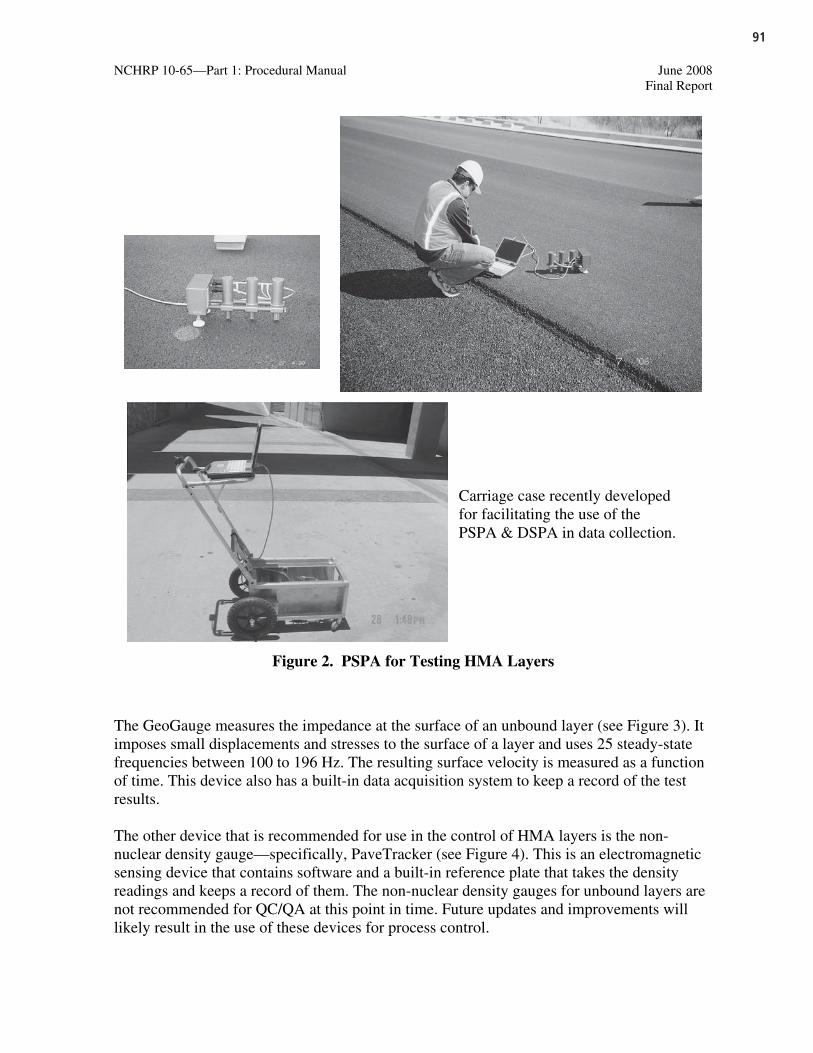
91
NCHRP 10-65—Part 1: Procedural Manual June 2008 Final Report
Figure 2. PSPA for Testing HMA Layers
The GeoGauge measures the impedance at the surface of an unbound layer (see Figure 3). It imposes small displacements and stresses to the surface of a layer and uses 25 steady-state frequencies between 100 to 196 Hz. The resulting surface velocity is measured as a function of time. This device also has a built-in data acquisition system to keep a record of the test results.
The other device that is recommended for use in the control of HMA layers is the non-nuclear density gauge—specifically, PaveTracker (see Figure 4). This is an electromagnetic sensing device that contains software and a built-in reference plate that takes the density readings and keeps a record of them. The non-nuclear density gauges for unbound layers are not recommended for QC/QA at this point in time. Future updates and improvements will likely result in the use of these devices for process control.
Carriage case recently developed for facilitating the use of the PSPA & DSPA in data collection.

92
NCHRP 10-65—Part 1: Procedural Manual June 2008 Final Report
Figure 3. Humboldt GeoGauge
Figure 4. Non-Nuclear Density Gauge, PaveTracker

93
NCHRP 10-65—Part 1: Procedural Manual June 2008 Final Report
3.1.1 Acceptance Plan
Different acceptance procedures are used in judging whether the pavement material meets the required specifications. Two methods used by most agencies are Percent Within Limits (PWL) and Average Absolute Deviation (AAD). This document uses PWL for determining acceptance and specification compliance. AASHTO R 9-03, Acceptance Sampling Plans for Highway Construction, is recommended for use in preparing practical but effective procedures that agencies can use in deciding whether the product meets their specifications (AASHTO 2003). AASHTO R 9-03 should be followed in determining the number of tests per lot, lot size, and other specifics of the acceptance sampling plan.
The upper and lower quality indices are calculated in accordance with Equations 1 and 2, respectively.
s
LSLXQL ................................................................................................................ (1)
s
XUSLQL ................................................................................................................ (2)
Where:
LQ = Lower quality index.
UQ = Upper quality index.
USL = Upper specification limit. LSL = Lower specification limit. s = Sample standard deviation of the lot. X = Sample mean of a lot.
The upper and lower quality indices are used to determine the total PWL for each lot of material using Equation 3. The upper and lower PWL values are then determined from the Q-tables provided in the AASHTO QC/QA Guide Specification.
100UL PWLPWLPWL ......................................................................................... (3)
Where: PWL = Percent Within Limits. PWLL = Percent Within Limits from the lower specification limit. PWLU = Percent Within Limits from the upper specification limit.
Determine the Combined Variability for HMA MixturesThe combined variability includes the within-process variability and the target-miss variability or the precision of the target value. A reasonable combined variability for the initial use in setting the specification is provided for both HMA and crushed aggregate base layers in latter parts of this document. The combined variability is expected to be dependent on the target stiffness of the material.

94
NCHRP 10-65—Part 1: Procedural Manual June 2008 Final Report
Agencies should develop agency-specific values based on reasonable standard care and workmanship of producing, placing, and compacting HMA layers. A minimum of 10 projects should be used to determine the combined variability for a range of mixtures. The within-process and center or target-miss variability should exclude areas with anomalies or construction defects.
Determine Specification Limits for an HMA MixtureEstablishing the specification limits for a specific mixture requires that the acceptable and unacceptable (defined as rejectable material) be defined. The acceptance and rejectable quality levels are dependent on the within-process variability. These all become engineering decisions of the agency and are used to determine the PWL for the different materials.
3.2.1 Quality Control Plan
Of the many process control procedures that can be used in highway construction, process control charts, particularly statistical control charts, are commonly used by contractors and material producers for verifying that their process is under control. Although there are different approaches that can be taken in implementing NDT technologies to verify that the process is in control, statistical control charts are being used within this document. The ASTM Manual on Presentation of Data and Control Chart Analysis was used for preparing practical procedures that contractors can use in deciding whether their process is in control (ASTM 1992).
The upper and lower control or action limits for the sample means are calculated in accordance with Equations 4 and 5.
sAXUCLX 3 ........................................................................................................ (4)
sAXLCLX 3 ........................................................................................................ (5)
Where:
XUCL = Upper control limit for the sample means.
XLCL = Lower control limit for the sample means.
X = Target value for a project. s = Pooled standard deviation that represents the process variance. A3 = Factor for computing control chart limits and dependent on the number of
observations in the sample.
The target value of the control chart for each material is the average modulus measured in the laboratory. Both action and warning limits are normally included on the statistical control charts. The upper and lower action limits are set at three standard deviations from the target value, while the warning limits are set at two standard deviations from the target.

95
NCHRP 10-65—Part 1: Procedural Manual June 2008 Final Report
The upper and lower control limits for the sample standard deviations are calculated in accordance with Equations 6 and 7, while Equations 8 and 9 are the limits when the range ( R ) is used.
sBUCLs 3 ................................................................................................................ (6)
sBLCLs 4 ................................................................................................................ (7)
RDUCLR 3 .............................................................................................................. (8)
RDLCLR 4 .............................................................................................................. (9)
Where: B3,4 = Factors for computing control chart limits based on sample standard
deviations and dependent on the number of observations in the sample. D3,4 = Factors for computing control chart limits based on the range within the
sample and dependent on the number of observations in the sample.
4.1 HMA MIXTURES AND LAYERS
4.1.1 Acceptance Testing of HMA Mixtures and Layers
The dynamic moduli measured in the laboratory and the moduli measured with the PSPA were found to have a normal distribution, excluding areas with construction defects. Thus, the assumption of normality is applicable but should be checked, especially for harsh and tender HMA mixtures.
Step 1: Determine JMF and Target Mixture Properties
A master curve for each HMA mixture included in the design strategy (new construction or rehabilitation with HMA overlays) is normally assumed for structural design. This assumed master curve or specific modulus values are used within the mixture design process for determining the job mix formula (JMF) to ensure that the mixture design satisfies the structural design assumptions. The materials selection and mixture design should be completed in accordance with NCHRP Project 9-33.
Step 2: Verify the JMF with Plant Produced Mixture
The HMA mixture JMF should be verified with a plant produced mixture. If minor revisions are needed to satisfy the design criteria, those revisions should be completed and confirmed prior to determining the target modulus value for acceptance. The procedures recommended within NCHRP Project 9-33 should be followed for making any revisions to the JMF to ensure that the assumptions used for structural design have been met.

96
NCHRP 10-65—Part 1: Procedural Manual June 2008 Final Report
Step 3: Determine Target Dynamic Modulus for HMA Mixture
a. After the HMA mixture design has been verified from plant produced material, dynamic moduli should be determined for the mixture compacted to the target density specified for the in-place mixture (93 to 94 percent compaction or percent maximum theoretical density). The target density or percent compaction should be established by the agency. These dynamic moduli are used to determine the seismic shift factor. The purpose of the seismic shift factor is to translate the seismic modulus into a design modulus (see step 5).
The test temperatures should include those that are expected during the acceptance testing of the mixture. The recommended temperatures include 90, 110, 130, and 150 °F (see Figure 5). Higher temperatures may need to be used if the acceptance testing is completed the same day of paving. The load frequencies used during testing should include 0.1, 0.5, 1.0, 5.0, and 10.0 Hz. If an approved master curve was already measured from the mixture plant verification process, it is not necessary to redo the test. The results from the earlier testing can be used.
Not all agencies have the laboratory equipment in their district or field laboratories for HMA mixtures. Two options are provided: one for the case where the equipment is available for measuring the dynamic moduli and the second for the case where that equipment is unavailable.
Option A—Measure Dynamic ModulusSample plant produced mixture from the control strip or at the beginning of the project and compact three test specimens using a Superpave gyratory compactor to the density or air void level targeted or specified. Dynamic moduli are measured on the approved, plant verified JMF in accordance with AASHTO TP 62 over the range of temperatures expected during acceptance testing.
Option B—Calculate Dynamic Modulus of HMA Mixture with Regression EquationsCalculate the dynamic modulus over the range of frequencies and temperatures selected in accordance with NCHRP Project 9-33 or NCHRP Report 465 (see Figure 5). Use of regression equations is considered permissible because adjustments need to be made for the specific mixture.
b. The target dynamic modulus is determined for a specific or reference frequency (5 Hz is suggested) and temperature (the mid-range temperature expected during acceptance testing is suggested). See step 5 for additional discussion on the reference frequency and temperature. The target dynamic moduli should be compared to the value used for structural design. If the measured or calculated modulus is significantly different than the assumed value at the same frequency and temperature, revisions should be made to the mixture or structural designs.

97
NCHRP 10-65—Part 1: Procedural Manual June 2008 Final Report
c. The test specimens used to verify the JMF and prepared for dynamic modulus testing are also used in step 4 for measuring the seismic modulus of the mixture at different temperatures.
Figure 5. HMA Dynamic Moduli, Measured in the Laboratory or Calculated UsingMEPDG Regression Equation
Dynamic Modulus Regression Equation
0.1
1
10
100
0.1 1 10 100
Frequency, Hz.
Dyn
amic
Mo
du
lus,
E x
105 p
si
70 F90 F110 130 150
Dynamic Modulus Regression Equation
0.1
1
10
100
60 70 80 90 100 110 120 130 140 150 160
Temperature, F
Dyn
amic
Mo
du
lus,
E x
105 p
si
0.5151025
`

98
NCHRP 10-65—Part 1: Procedural Manual June 2008 Final Report
Step 4: Measure Laboratory Seismic Modulus on Plant Produced Mixture
The seismic modulus should be measured in accordance with ASTM D 5345. The seismic modulus can be measured on those test specimens that were prepared for the mixture verification process (see step 2), as long as they were compacted to the expected or specified in-place target density or air void level. The seismic modulus is measured on test specimens for each temperature selected under step 3 using a device, known as a V-meter, containing a pulse generator and a timing circuit, coupled with piezoelectric transmitting and receiving transducers (see Figure 6). The timing circuit digitally displays the time needed for a wave to travel through the test specimen. The measured travel time, the dimensions, and the mass of the test specimen are used to calculate the modulus.
The free-free resonant column (FFRC) test is a laboratory test to measure the modulus of the HMA mixture during the mixture design and field verification process. A cylindrical specimen is subjected to an impulse load at one end. Seismic energy over a large range of frequencies will propagate within the specimen. Depending on the dimensions and the stiffness of the specimen, energy associated with one or more frequencies are trapped and magnified (resonate) as they propagate within the specimen. The goal with this test is to determine these resonant frequencies. Since the dimensions of the specimen are known, if one can determine the frequencies that are resonating (i.e., the resonant frequencies), one can readily calculate the modulus of the test specimen.
Figure 6. Equipment for Measuring the Seismic Modulus of Laboratory Compacted Test Specimens

99
NCHRP 10-65—Part 1: Procedural Manual June 2008 Final Report
The seismic modulus should be translated into a design modulus (see Figure 7). This step is necessary because seismic moduli are low-strain, high-strain-rate values, whereas the design moduli are based on low-strain, low-strain-rate values. The method of calculating the design modulus is to develop a master curve based on the recommendations of NCHRP Report 465, "Simple Performance Test for Superpave Mix Design," or in accordance with the NCHRP Project 9-33 mixture design procedure.
Figure 7. Graphical Illustration for Shifting the Seismic Moduli to the Dynamic Moduli for a Specific Load Frequency Using the Mixture Master Curve
Select the mat temperatures that are expected during the acceptance testing (see step 3). Typical values that can be used include 90, 110, 130, and 150 °F. The seismic shift factor is determined using Equation 10.
TTc
TTcaLog
o
oT
2
1 (10)
Where: c1 = Regression coefficient determined from the dynamic modulus tests or
calculations (for neat mixtures this value has been reported to be 19 and for polymer modified asphalt mixtures the value is 17.44).
1
10
100
1000
1E-02 1
Seismic
Design Frequency
Design Modulus
10000
1E-04 1E+02
Frequency (Hz)
Mod
ulu
s (k
si)
1E+06 1E+081E+04
Step 5: Determine Seismic Shift Factor to Translate the Seismic Modulus into the Design Modulus

100
NCHRP 10-65—Part 1: Procedural Manual June 2008 Final Report
c2 = Regression coefficient determined from the dynamic modulus tests or calculations (for neat mixtures this value has been reported to be 92, while for polymer modified mixtures this value is 51.6).
To = Reference temperature, which should be the median value expected during acceptance testing.
T = Test temperature.
Equation 10 is used to translate the PSPA seismic moduli measured at varying surface temperatures during acceptance testing to the design modulus at the reference temperature and frequency. The reference temperature should be the approximate mid-range temperature during acceptance testing. Using the mid-range temperature should reduce or minimize potential bias that could be present if always translating to a higher or lower temperature.
The seismic shift factors are entered in the PSPA software to adjust the seismic values to the design frequency selected (see Figure 7). It is recommended that a load frequency of 5 Hz be used to determine the design modulus. However, the agency can select other frequencies to be consistent with the posted speed limit of the project—an input to the MEPDG.
Step 6: Determine the Field Adjustment Factor (Adjusting Field to Laboratory Conditions)
This step is to determine the field ratio for adjusting the design moduli to laboratory conditions. In other words, that ratio should be used to adjust the design moduli measured with the PSPA to laboratory conditions.
a. Select 8 to 10 random locations within the control strip or first day’s production and measure the PSPA modulus and surface temperatures in accordance with step 7.
b. Drill and recover cores at a minimum of three locations. One core should be recovered from a location where the higher seismic modulus was measured, one at the location of the lowest seismic modulus, and the third at the median modulus value.
c. Measure the bulk specific gravity (Gmb) of each core from the HMA mat in accordance with AASHTO T 166.
d. Measure the maximum specific gravity (Gmm) of each core in accordance with AASHTO T 209.
e. Calculate the air void level (Va) of each core in accordance with AASHTO T 269 and determine the percent compaction using Equation 11.
aVCompaction 100% (11)
f. Calculate or measure the dynamic modulus of the mixture using the average air void level measured from the three field cores.

101
NCHRP 10-65—Part 1: Procedural Manual June 2008 Final Report
g. Determine the specific adjustment ratio for the mixture in accordance with Equation 12.
Design
Lab
E
ER
*
(12)
h. Determine if the field ratio deviates significantly from values near unity. The following provides a summary of the average ratios that have been measured on other HMA mixtures. It is expected that the ratio should be within three standard deviations. If the field ratio is outside three standard deviations from the mean value, it is expected that a significant change has occurred to the mixture between field verification and production. If the values are outside three standard deviations from those listed in Table 1, the mixture should be evaluated in more detail to ensure that the values are correct.
Field Adjustment Ratios HMA Mixture Type
MeanStandardDeviation
High binder content mixtures that exhibit tenderness, including SMA type mixtures
0.89 0.153
Harsh mixtures, coarse-graded mixtures including PMA
1.34 0.231
Table 1. Summary of the Average Ratios That Have Been Measured on Other HMA Mixtures
Step 7: Acceptance Testing with the PSPA for Measuring Modulus of HMA Mixtures
a. Allow the mixture to cool prior to using the PSPA. Elevated temperatures can cause the rubber pads on the tips of the receivers to melt. The test should be performed on areas with surface temperatures less than 200°F. The PSPA test should be performed in accordance with the manufacturer’s recommendations.
b. Remove any loose material on the surface. The receivers or sensors should be in direct contact with the test surface.
c. Place the PSPA on the HMA surface. Align the sensor bar parallel to the direction of the paver and rollers. Slightly push the sensor bar to ensure that the receivers are in good contact with the surface. If mat tears or checking is observed in the test area, the PSPA should not be moved; the test should be conducted on that area, regardless of the surface condition.
d. After seating the PSPA, activate the software. Enter the type of surface tested and the mat thickness into the software. Inspect the graphical display of the load response and receivers on the screen of the laptop. If the load pulse has an irregular shape, repeat the test. One of the receivers may not be in good contact with the surface.

102
NCHRP 10-65—Part 1: Procedural Manual June 2008 Final Report
e. Record the seismic-design modulus and surface temperature reported by the PSPA.
f. Lift and rotate the PSPA 90° to the first direction of testing and repeat steps b to d.
g. Lift and rotate the PSPA by 45° between the first two readings and repeat steps b to d.
Step 8: Determine the Combined Variability for Setting the Specification Limits
The specification limits are defined by the combined variability for the HMA. Most agencies will have insufficient data to date for estimating this value in terms of setting the specification limits. Based on multiple operators and gauges, the following provides the recommended combined variability for dense-graded HMA mixtures to be used until sufficient data become available (based on the number of tests recommended above).
Dynamic Modulus Combined Variability = 95 ksi
The target dynamic modulus for the specifications was defined under step 3.
Step 9: Determine Quality Indices and PWL for a Lot
The upper and lower quality indices are calculated in accordance with Equations 1 and 2, respectively, and used to determine the total PWL for each lot of material using Equation 3. The upper and lower PWL values are then determined from the Q-tables provided in the AASHTO QC/QA Guide Specification.
4.2.1 Quality Control Testing of HMA Mixtures and Layers
The quality control plan uses the non-nuclear density gauges. The PaveTracker gauge was specifically used to determine the control limits and other required information; that gauge is referred to specifically within this document, but other non-nuclear density gauges can be used if found to be acceptable.
Step 1: Determine the Density Correction Factor for the Non-Nuclear Density Gauge Used for Process Control
a. The density of the HMA mat should be measured with the PaveTracker device at each of the 8 to 10 locations selected for seismic testing within the control strip of the first day’s production (see Acceptance Testing).
b. Determine the average density correction factor (DCF) between the PaveTracker density values and the densities (bulk specific gravities) measured on the field cores.
Gauge
CoreDCF or )(
)(
Gaugemb
Coremb
G
G
γγ
(13)

103
NCHRP 10-65—Part 1: Procedural Manual June 2008 Final Report
It is recommended that a contractor take a total of five cores at the beginning to increase the sample size for determining the average density correction factor. As the contractor becomes more familiar with the non-nuclear density gauges, that number for the control strips can be reduced to three for most mixtures. In addition, make sure that the surface is dry when establishing the DCF.
c. The densities measured with the PaveTracker or other non-nuclear density gauges are multiplied by the DCF to obtain the in-place density.
Step 2: Establish Density-Growth Curve and Temperature Sensitive Zone
a. At the beginning of the paving process, it is recommended that a density-growth curve be developed for the specific mixture and compaction train being used.
b. Measure the density after each pass of the roller over a specific point, in at least two locations or test points. Two readings should be taken at each point, and the average value recorded and used to determine the DCF. The surface temperature should also be recorded after each pass of the roller used in the compaction train—including the finish roller(s). The reason for reducing the number of density measurements in developing the density-growth curve is avoid delaying the compaction operation of the rollers. If time permits between each roller pass over a specific point, a minimum of three readings should be taken and the average value used.
c. A density-growth curve should be prepared for each test point used during the control strip or first day’s production (see Figure 8). This testing is recommended for two reasons:
To determine the number of passes of each roller for obtaining the target or specified density level. To determine whether the rollers will be operating within the temperature sensitive zone, and if so, to determine the temperature range through which the rollers should be restricted from rolling the mat (see Figure 9). Rolling within the temperature sensitive zone can significantly reduce the density of the HMA mat and cause the mat to check and tear. If this condition occurs, the owner agency will likely require that the mat be removed and replaced.
Step 3: Process Control Testing with Non-Nuclear Density Gauges
a. The non-nuclear density gauge should be operated according to the manufacturer’s recommendations.
b. If the surface is wet (free water or water ponded on the surface), all free water should be removed and the surface allowed to dry in the area of the test prior to taking any readings.

104
NCHRP 10-65—Part 1: Procedural Manual June 2008 Final Report
c. Determine the number of test points per lot and sublot for controlling the HMA compaction. As a minimum, it is recommended that three test points per sublot be used for process control. The lot should be determined based on other tests being used by the contractor for process control (i.e., sampling the mixture for volumetric property determination using the gyratory compactor in the field or plant laboratory).
d. Identify or mark the area to be tested within each sublot.
e. Take four readings around the sides of each test point or test location. The gauge should be oriented in the same direction for each reading—in the direction of the paver and rollers is recommended. After the first reading, lift the gauge and move it to the next consecutive or adjacent side of the test point. Repeat until all sides of the test point have been taken. All four readings should be taken within a 1- to 2-foot square area.
f. Record all four readings and the surface temperature at each test point, and average the values for the test point.
145
147
149
151
153
155
157
159
161
163
165
0 1 2 3 4 5
Number of Roller Passes
Den
sity
Mea
sure
d w
ith
Pav
eTra
cker
, pcf
170
180
190
200
210
220
230
Tem
per
atu
re o
f M
ixtu
re, F
Mat Density Joint Density Mat Temperature Joint Temperature
Figure 8. Density-Growth Curve Measured with the PaveTracker
Step 4: Determine the Combined Variability for Setting the Control Limits
The control limits are defined by the contractor’s within-process variability of density for HMA. Most contractors should have sufficient data for estimating this value in terms of setting the action and warning limits for the statistical control charts. Based on multiple operators and gauges, the following provides the recommended pooled standard deviation for density of the non-nuclear density gauges (PaveTracker), excluding all areas with anomalies and those areas where mat checking and tearing were exhibited.

105
NCHRP 10-65—Part 1: Procedural Manual June 2008 Final Report
Pooled Standard Deviation for Density = 2.5 pcf
146.0
148.0
150.0
152.0
154.0
156.0
158.0
0 2 4 6 8 10 12
Number of Passes of the Rollers
Den
sity
of
Mat
Mea
sure
d w
ith
Pav
eTra
cker
, pcf
200
210
220
230
240
250
260
Tem
per
atu
re o
fM
ixtu
re, F
Density Temperature
Figure 9. Density-Growth Curve Showing the Effects of Rolling within the Temperature Sensitive Zone
5.1 UNBOUND MATERIALS AND LAYERS
5.1.1 Acceptance Testing for Unbound Materials and Layers
The resilient moduli measured in the laboratory and the moduli measured with the GeoGauge were found to have a normal distribution, excluding areas with construction defects.
Step 1: Determine the Moisture-Density Relationship of the Soil and Material
Determine the moisture-density (M-D) relationship of the unbound material or soil in accordance with AASHTO T 180. The optimum water content and maximum dry density are the target values for determining the resilient modulus of the unbound layer.
Step 2: Determine Target Resilient Modulus
The target value for acceptance should be the average resilient modulus used as the input to the MEPDG. This value may have been determined from other physical properties and may or may not relate to the optimum water content and maximum dry unit weight of the material.
The resilient modulus, however, should be determined in the laboratory on test specimens prepared and compacted to the target density specified for the in-place mixture (100 percent of the maximum dry density as determined by AASHTO T 180). The target density should be

106
NCHRP 10-65—Part 1: Procedural Manual June 2008 Final Report
established by the agency. The resilient modulus determined for the specified density and water content is the target resilient modulus for process control (see Figures 10 and 11). This target resilient modulus may or may not be the target value for acceptance.
Not all agencies have the laboratory equipment in their district or field laboratories for measuring the resilient modulus of the unbound layers. Thus, two options are provided: one for the case where the repeated load resilient modulus measuring equipment is available and the second for the case where that equipment is unavailable.
Option A—Measure Resilient ModulusSample the unbound materials from the stockpiles or from the control strip and compact three test specimens. Measure the resilient modulus of the unbound material over the range of stress states in accordance with AASHTO T 307. Determine the target resilient modulus at a low confining pressure and repeated vertical stress suggested below.
Layer & Material Type Confinement,
psiRepeatedStress, psi
Total Vertical Stress, psi
Subgrade; Fine-Gained Soils with Plasticity
2 2 4
Embankment; Soil-Aggregate Mixture
4 4 8
Crushed Aggregate Base 6 6 12
Table 2. Option A—Measure Resilient Modulus
Figure 10. Resilient Modulus Measured in the Laboratory for a Crushed Stone Base Material
10000
30000
50000
70000
90000
110000
130000
0.0 10.0 20.0 30.0 40.0 50.0 60.0 70.0 80.0 90.0 100.0
Bulk Stress, psi
Res
ilien
t M
od
ulu
s, p
si
Confinement = 3 psi Confinement = 6 psi Confinement = 10 psi
Confinement = 15 psi Confinement = 20 psi

107
NCHRP 10-65—Part 1: Procedural Manual June 2008 Final Report
Figure 11. Resilient Modulus Measured in the Laboratory for a Crushed Stone or Aggregate Base Material
Option B—Calculate Resilient Modulus of the Unbound Material with Regression EquationsCalculate the resilient modulus for the stress states listed above in accordance with one of the regression equations from the Federal Highway Administration (FHWA) Long Term Pavement Performance (LTPP) program. These regression equations are shown below. Use of the regression equations is considered permissible because adjustments need to be made for the specific material.
32
11
k
a
oct
k
aaR pp
pkMθ
θθ
τ
τ
τ
σ
σ
σ σ σ σ σ σ
σ σ
(14)
Where: = Bulk Stress, psi
321 15)
= Octahedral shear stress, psi
3
5.0213
232
221
(
(16)
ap = Atmospheric pressure, 14.7 psi.
3,2,1 = Principal stress, psi.
3,2,1k = Regression constants from laboratory resilient modulus test results.
10
20
30
40
50
60
70
80
90
0 10 20 30 40 50 60 70 80 90 100
Bulk Stress, psi
Res
ilien
t M
od
ulu
s, k
si
Confinement = 3 psi Confinement = 6 psi Confinement = 10 psi
Confinement = 15 psi Confinement = 20 psi

108
NCHRP 10-65—Part 1: Procedural Manual June 2008 Final Report
The k regression constants are material specific. The following defines the regression constants for the different materials that were tested within the field evaluation projects. These relationships for these regression constants were developed from the FHWA-LTPP study (Von Quintus and Killingsworth 1998)
Crushed Stone Base Materials:
dryswLL γ
γ
γγ
γ
γ
γ
γγ
γγ
γγ
γ
γ
γγ
Pk 0001.0037.00088.0008.07632.0 8/31 (17)
40#
2
8/32
00000024.00006.0
038.00008.00016.02159.2
P
wLLPk
drydry
s
(18)
dryswLLk 0005.00014.00082.01720.13 (19)
Embankments, Soil-Aggregate Mixture, Coarse-Grained
40#
2
200#4#8/31
00000082.0
3932.06456.10426.00000016.0
0149.00027.00174.00130.05856.0
P
w
ww
PIPPPk
Max
Max
s
Max
drySMax (20)
40#
2
200#2
00000027.0
1483.00001.00081.00060.07833.0
P
w
wPIPk
dry
opt
sMax
(21)
40#
2
200#3 00000081.00026.01906.0P
Pk opt (22)
Embankments, Soil-Aggregate Mixture, Fine-Grained
Max
dryoptw
LLPPk
179.1051.0
0030.00128.00051.07668.0 200#4#1
(23)
Max
dryPPk 3941.10061.00141.04951.0 200#4#2 (24)
Max
dryLLPk 8903.30036.00293.09303.0 8/33 (25)

109
NCHRP 10-65—Part 1: Procedural Manual June 2008 Final Report
Fine-Grained Clay Soil
swClayk 0437.00106.03577.11 (26)
swLL
PPPk
0049.00030.0
0027.00095.00073.05193.0 200#40#4#2 (27)
opt
sdryopt w
wwLL γ γ
SiltPPPk
6055.00025.00026.00672.00535.0
025.00521.00303.00288.04258.1
max
200#40#4#3
(28)
Step 3: Determine the Field Adjustment Factor (Adjusting Field to Laboratory Conditions)
The GeoGauge results in a field modulus and needs be adjusted to be consistent with the structural design assumptions based on laboratory resilient modulus. This step is to determine the field ratio for adjusting the GeoGauge measurements to laboratory conditions. Once this field ratio or factor is determined, that ratio should be used to adjust the GeoGauge modulus to laboratory conditions for all readings.
a. At a minimum of two locations within the control strip or first day’s production, use the GeoGauge to measure the increase in modulus of the material under the roller. In other words, develop a modulus-growth curve (see Figure 12). The number of passes of the roller should be increased until the modulus remains the same.
b. Select 8 to 10 random locations within the control strip or first day’s production and measure the GeoGauge modulus in accordance with step 7.
c. Measure the density and moisture content at three of these locations using the sand-cone test to ensure that the material has been compacted to the dry density established by the agency’s specifications.
d. Calculate or measure the resilient modulus of the in-place material using the average density and moisture contents measured from the sand-cone tests.
e. Determine the specific field ratio for the layer in accordance with the following equation.
DesignM
LabMR
R
RResilient Modulus (29)
f. Determine if the field ratio deviates significantly from values near unity. The following provides a summary of the average ratios that have been measured on other unbound materials. It is expected that the ratio should be within three standard deviations. If the adjustment ratio is outside three standard deviations from the mean value, it is expected that a significant change has occurred to the material between field calibration and production. If the values are outside three standard deviations

110
NCHRP 10-65—Part 1: Procedural Manual June 2008 Final Report
from those listed below, the material should be evaluated in more detail to ensure that the values are correct.
Field Adjustment Ratios for Aggregate Base Materials and Soil-Aggregate Mixtures for Embankments:
Mean Value = 1.031 Standard Deviation = 0.370
Figure 12. Modulus-Growth Curve Measured with the GeoGauge
Step 4: Use GeoGauge for Measuring Modulus of Unbound Layers for Acceptance and Conformance
a. The material modulus should be measured on the in-place material using the GeoGauge in accordance with the manufacturer’s recommendations.
b. Remove any loose material on the surface, being careful not to disturb or remove an excessive amount of material. Figure 3 shows the tools that can be used to clean the test surface.
c. Place the moist sand on the test surface and pad it into place to fill any surface voids. The layer of moist sand should just cover the test surface and be sufficient in area so that three different readings of the GeoGauge can be made within this test area. This area should be about 1 to 2 square feet in size. This thin, moist sand layer is to ensure that the bottom ring of the GeoGauge is in contact with the surface for at least 75 percent of it surface area.
d. Place the GeoGauge on the surface of the sand. Lightly twist the GeoGauge, but do not push the GeoGauge into the test material. The bottom plate of the GeoGauge (not the bottom of the ring) must not be in contact with the material being tested. After the
5
10
15
20
25
30
0 2 4 6 8 10 12
Number of Roller Passes
Res
ilien
t M
od
ulu
s fr
om
ND
T D
evic
es, k
si
DCP GeoGauge Log. (GeoGauge) Log. (DCP)

111
NCHRP 10-65—Part 1: Procedural Manual June 2008 Final Report
test, the surface of the layer should be inspected to ensure that it was not in contact with the GeoGauge.
e. Take a reading of the GeoGauge and record the modulus displayed. These readings can be stored in the device and downloaded at the end of the lot testing.
f. Adjust the readings externally to determine the laboratory equivalent resilient modulus values read by the GeoGauge.
g. Lift the GeoGauge and observe the surface of the thin layer of sand and test area. The thin layer of sand or test surface should not be indented by the gauge such that the bottom of the GeoGauge was in contact with the surface. If that was the case, the test result should be so noted and not used in the acceptance testing and the test repeated in a different area of the test area.
h. Move it to a different area with the sand layer and repeat steps d to g.
i. Lift the GeoGauge and move it to a third location and repeat steps d to g.
Step 5: Determine the Combined Variability for Setting the Specification Limits
The specification limits are defined by the combined variability for the unbound layers. Most agencies will have insufficient data to date for estimating this value in terms of setting the specification limits. Based on multiple operators and gauges, the following provides the recommended combined variability for dense-graded crushed stone base layers to be used until sufficient data become available (based on the number of tests recommended above).
Resilient Modulus Combined Variability = 3.10 ksi
The target resilient modulus for the specifications was defined under step 2 and is the value assumed and used as an input to the MEPDG.
Step 6: Determine Quality Indices and PWL for a Lot
The upper and lower quality indices are calculated in accordance with equations 1 and 2, respectively, and used to determine the total PWL for each lot of material using equation 3. The upper and lower PWL values are then determined from the Q-tables provided in the AASHTO QC/QA Guide Specification.
5.2.1 Quality Control Testing of Unbound Materials and Layers
The quality control plan uses the GeoGauge to determine the control limits and other required information. The non-nuclear electrical density gauges require future improvements for use in process control. Thus, most of the steps included for acceptance testing also apply to process control, with the following exceptions.

112
NCHRP 10-65—Part 1: Procedural Manual June 2008 Final Report
The target value of the control chart for the unbound layers is the average value measured in the laboratory in accordance with AASHTO T 307 and compacted to the specified density and water content specified by the agency.
Both action and warning limits are normally included on the statistical control charts. The upper and lower action limits are set at three standard deviations from the target value, while the warning limits are set at two standard deviations from the target. The pooled standard deviation used to set the control limits will be contractor and material specific. The following provides the overall pooled standard deviation until contractors develop sufficient information and data for setting their own control limits.
Overall pooled standard deviation for setting the limits of statistical control charts for process control = 3.10 ksi
Abbreviations and acronyms used without definitions in TRB publications:
AAAE American Association of Airport ExecutivesAASHO American Association of State Highway OfficialsAASHTO American Association of State Highway and Transportation OfficialsACI–NA Airports Council International–North AmericaACRP Airport Cooperative Research ProgramADA Americans with Disabilities ActAPTA American Public Transportation AssociationASCE American Society of Civil EngineersASME American Society of Mechanical EngineersASTM American Society for Testing and MaterialsATA Air Transport AssociationATA American Trucking AssociationsCTAA Community Transportation Association of AmericaCTBSSP Commercial Truck and Bus Safety Synthesis ProgramDHS Department of Homeland SecurityDOE Department of EnergyEPA Environmental Protection AgencyFAA Federal Aviation AdministrationFHWA Federal Highway AdministrationFMCSA Federal Motor Carrier Safety AdministrationFRA Federal Railroad AdministrationFTA Federal Transit AdministrationIEEE Institute of Electrical and Electronics EngineersISTEA Intermodal Surface Transportation Efficiency Act of 1991ITE Institute of Transportation EngineersNASA National Aeronautics and Space AdministrationNASAO National Association of State Aviation OfficialsNCFRP National Cooperative Freight Research ProgramNCHRP National Cooperative Highway Research ProgramNHTSA National Highway Traffic Safety AdministrationNTSB National Transportation Safety BoardSAE Society of Automotive EngineersSAFETEA-LU Safe, Accountable, Flexible, Efficient Transportation Equity Act: A Legacy for Users (2005)TCRP Transit Cooperative Research ProgramTEA-21 Transportation Equity Act for the 21st Century (1998)TRB Transportation Research BoardTSA Transportation Security AdministrationU.S.DOT United States Department of Transportation