NBER WORKING PAPER SERIES

HOW LARGE ARE THE SOCIAL RETURNS TO EDUCATION? EVIDENCE FROM

COMPULSORY SCHOOLING LAWS

Daron AcemogluJoshua Angrist

Working Paper 7444http://www.nber.org/papers/w7444

NATIONAL BUREAU OF ECONOMIC RESEARCH1050 Massachusetts Avenue

Cambridge, MA 02138December 1999

We thank Chris Mazingo and Xuanhui Ng for excellent research assistance. Paul Beaudry, Bill Evans, BobHall, Larry Katz, Enrico Moretti, Jim Poterba, Robert Shimer, and seminar participants at the 1999 NBERSummer Institute, University College London, the University of Maryland, and the University of Torontoprovided helpful comments. Special thanks to Stefanie Schmidt for helpful advice on compulsory schoolingdata. The views expressed herein are those of the authors and not necessarily those of the National Bureauof Economic Research.

© 1999 by Daron Acemoglu and Joshua Angrist. All rights reserved. Short sections of text, not to exceedtwo paragraphs, may be quoted without explicit permission provided that full credit, including © notice, is givento the source.

How Large are the Social Returns to Education?Evidence from Compulsory Schooling LawsDaron Acemoglu and Joshua AngristNBER Working Paper No. 7444December 1999JEL No. I20, J31, J24, D62, O15

ABSTRACT

Average schooling in US states is highly correlated with state wage levels, even after controlling

for the direct effect of schooling on individual wages. We use an instrumental variables strategy to

determine whether this relationship is driven by social returns to education. The instrumentals for average

schooling are derived from information on the child labor laws and compulsory attendance laws that

affected men in our Census samples, while quarter of birth is used as an instrument for individual schooling.

This results in precisely estimated private returns to education of about seven percent, and small social

returns, typically less than one percent, that are not significantly different from zero.

Daron Acemoglu Joshua AngristDepartment of Economics Department of EconomicsMIT, E52-371 MIT, E52-35350 Memorial Drive 50 Memorial DriveCambridge, MA 02142 Cambridge, MA 02142and NBER and NBERdaron@mit.edu angrist@mit.edu

1 Introduction

Many studies …nd that an additional year of schooling increases individual wages by 6-10

percent. The economic consequences of a change in average schooling may di¤er from

this private return, however. Changes in average education levels raise wages by less than

the private returns to schooling if schooling has signaling value in addition to raising

productivity, or if some other factor of production is inelastically supplied. On the other

hand, the value of education to society may exceed the private return because of positive

social returns due to changes in relative wages, or human capital externalities from a

more educated labor force. Despite the potential importance of this question for economic

policy, much less is known about the social returns to education than the private returns.

In this paper, we develop a framework for estimating social returns by investigating the

e¤ect of state average schooling levels on individual wages, while controlling for the e¤ect

of individual schooling.

The principal challenge in any e¤ort to estimate the e¤ects of education on wages is

identi…cation. Individual education and average schooling levels are correlated with wages

for a variety of reasons, so the observed association between schooling variables and wages

is not necessarily causal. To solve this problem, we use instrumental variables to estimate

the e¤ect of both individual schooling and the average schooling level in an individual’s

state. The instruments for average schooling are derived from compulsory attendance laws

and child labor laws in states of birth. Together we refer to these as Compulsory Schooling

Laws (CSLs). The problem of estimating social returns is complicated by the fact that

there are two endogenous regressors a¤ected by CSLs, individual schooling and average

schooling. This problem is solved by using quarter of birth dummies as instruments for

individual schooling, as in Angrist and Krueger (1991), while using CSLs as instruments

for average schooling.

State CSLs generate an attractive “natural experiment” for the estimation of social

returns for a number of reasons. Although these laws were determined by social forces in

the states at the time of passage, the CSLs that a¤ected an individual in childhood are not

a¤ected by future wages. We also show that CSLs a¤ected schooling almost exclusively

in middle school and high school grades. This suggests that CSLs are not correlated with

omitted state-of-birth and cohort e¤ects, since these e¤ects would likely be related to

college-going behavior as well. Finally, changing CSLs were part of the 1910-1940 “high

school movement” that Goldin (1998) has argued was responsible for much of the human

capital accumulation in the US in the twentieth century.

The bulk of the empirical work in the paper uses samples of white men aged 40-49 from

the 1960-80 Censuses, although some estimates are computed using an extended sample

that includes 1950 and 1990 data. Blacks are excluded from the estimation because

cohorts of blacks in these data sets experienced marked changes in school quality (see,

e.g., Card and Krueger, 1992a; Margo, 1990; Welch, 1973). We focus on the 1960-80

Censuses because they include information on quarter of birth and because the census

schooling variable changes in 1990. The fact that men in their 40s are on a relatively

‡at part of the age-earnings pro…le also facilitates the use of quarter of birth dummies as

instruments.

OLS estimates using data from the 1960-80 Censuses show a large positive relationship

between average schooling and individual wages. A one-year increase in average schooling

is associated with about a 7 percent increase in average wages, over and above the roughly

equal private returns. In contrast with the OLS estimates, IV estimates of social returns in

1960-80 are typically less than one percent, and signi…cantly lower than the corresponding

OLS estimates. Adding data from the 1990 Census results in somewhat larger estimates

of social returns, but this …nding seems to be generated at least in part by problems with

the schooling variable in the 1990 Census.

In addition to having theoretical e¤ects on overall wage levels, exogenous changes

in average schooling may change the private returns to schooling. Changes in average

schooling caused by compulsory schooling laws provide an attractive source of variation

to estimate the e¤ect of supply shocks on the private returns to schooling. We explore

this issue by simultaneously estimating social returns and changes in private returns to

schooling. The results of this analysis also provide no evidence for signi…cant social

returns. They do suggest, however, that the returns to education may actually go up

when state average education increases.

Previous studies of the social returns to education include Rauch (1993), Mare (1995),

Peri (1998), and Moretti (1999), who estimate the e¤ect of average schooling in US cities

on individual wages, and Topel (1999), who estimates social returns using cross-country

data on education and labor productivity. Rauch, Mare, and Peri treat both individual

and average schooling variables as exogenous. In contrast, Moretti (1999) instruments

for average schooling with changes in city age structure, tuition costs and the presence

of a land-grant college, though he treats individual schooling as exogenous. We show

2

that instrumenting average schooling but not individual schooling may also be misleading

if instrumental variables (IV) estimates of private returns di¤er from OLS estimates.

Another di¤erence between our paper and Moretti’s is that compulsory schooling laws

mainly a¤ected pupils in middle school or high school, while most of the variation in

Moretti’s sample comes through changes in college attendance and graduation.

The next section lays out a simple economic model that shows how human capital

externalities can generate social returns to schooling. We focus on human capital exter-

nalities because they play an important role in recent discussions of economic growth (e.g.,

Lucas, 1988). The model is used to develop an estimation framework and to highlight

the econometric issues raised in attempts to separate private from social e¤ects. Section 3

discusses the data and reports OLS estimates from regressions on individual and average

schooling. Section 4 describes the CSL instruments, Section 5 reports the IV estimates,

and Section 6 estimates the impact of greater supply of education on private returns to

schooling.

2 Social returns: theory and measurement

2.1 Theoretical framework

A model similar to Acemoglu (1996) is used to highlight the economic forces that may

generate social returns to education, and to derive an estimating equation. Consider an

economy lasting two periods, with production only in the second period, and a continuum

of workers normalized to 1. An individual’s human capital is given by

hi = exp(´i ¢ si);

where si is worker i’s schooling. Workers have unobserved ability ´i = µi´(si), which

depends on an individual characteristic, µi, and also potentially on schooling. This de-

pendence captures potential decreasing returns to individual schooling, as in Lang (1993).

A worker’s consumption, Ci, is equal to his labor income. Schooling is chosen by

workers so as to maximize

lnCi ¡ 12Ãi ¢ s2i : (1)

The parameter Ãi is the cost of education for individual i and can be interpreted as a

personal discount rate, along the lines of Card (1995a).

3

There is also a continuum of risk-neutral …rms. In period 1, …rms make an irreversible

investment decision, k, at cost rk. Workers and …rms come together in the second period.

The labor market is not competitive; instead, …rms and workers are matched randomly,

and each …rm meets a worker. The only decision workers and …rms make after matching is

whether to produce together or not to produce at all (since there are no further periods).

If …rm j and worker i produce together, their output is

k®j ¢ hºi (2)

where ® < 1, º · 1 ¡ ®, and the worker receives a share ¯ of this output as a result ofbargaining.

An equilibrium in this economy is a set of schooling choices for workers and a set of

physical capital investments for …rms. Firm j maximizes the following expected pro…t

function:

(1¡ ¯) ¢ k®j ¢ E[hºi ]¡ r ¢ kj ; (3)

with respect to kj. Since …rms do not know which worker they will be matched with,

their expected pro…t is an average of pro…ts from di¤erent skill levels. The function (3) is

strictly concave, so all …rms choose the same level of capital investment, kj = k, given by

k =

µ(1¡ ¯) ¢ ® ¢H

r

¶1=(1¡®)(4)

where

H ´ E[hºi ] = E[exp(º ¢ ´i ¢ si)]

is the measure of aggregate human capital. Substituting (4) into (2), and recalling that

wages are equal to a fraction ¯ of output, the wage income of individual i is given by

Wi = ¯³(1¡¯)®H

r

´®=(1¡®)(exp(´isi))

º. Taking logs, this is:

lnWi = c+®

1¡ ® lnH + º´isi; (5)

= c+®

1¡ ® lnH + º lnhi;

where c is a constant and ®1¡® and º are positive coe¢cients.

1

1As in Acemoglu (1996), human capital externalitites are additive in logs, so the marginal product ofa more skilled worker increases when the average workforce skill level increases. Acemoglu (1998, 1999)discuss models in which log wage di¤erences between skilled and unskilled workers increase with averageskill levels.

4

Human capital externalities arise here because …rms choose their physical capital in

anticipation of the average human capital of the workers they will employ in the future.

Since physical and human capital are complements in this setup, a more educated labor

force leads to greater investment in physical capital and to higher wages. In the absence

of the need for search and matching, …rms would immediately hire workers with skills

appropriate to their investments, and there would be no human capital externalities.2

The model is completed by individual schooling decisions, which are determined by

maximizing (1), taking (5) as given. This yields equilibrium schooling levels satisfying

ºµi [´(si) + si´0(si)] = Ãisi, or (6)

´0(si)¡"¡1´ + 1

¢=

Ãiºµi;

where "´ is the elasticity of the function ´. The population average return to optimally

chosen schooling levels is E[ºµi(´i(si) + si´0i(si))]. But the average return for particular

subpopulations interacts with discount rates in a manner noted by Lang (1993) and Card

(1995a). For example, if ´0(si) < 0, those with high Ãi will get less schooling, and a

marginal year of schooling will be worth more to such people than the population average

return.

Equation (5) provides the theoretical basis for our empirical work. Since H is unob-

served, however, we use the following approximation to write lnH as a function of average

schooling:

lnH = lnE[exp(º´isi)] ¼ c0 + c1E(´isi) ¼ c2 + c3E(si):

The …rst step approximates the mean of the log with the log of the mean. The second step

takes E(´i) and the covariance between ´i and si to be constant, una¤ected by changes

in average education. Estimation can therefore be based on the following equation for

individual i residing in state j:

lnWij ¼ °0 + °1Sj + °2´isi (7)

where Sj = E(si) is average schooling in state j.

The scenario outlined here is not the only mechanism that might generate a relation-

ship like (7). One possibility, noted by Marshall (1964), Jacobs (1970), and Lucas (1988),

2In a frictionless world, …rms maximize pro…ts conditional on realized worker-…rm matches insteadof conditional on the expected match. In this case, …rm j matched to worker i chooses capital kj =³®hºir

´1=(1¡®)and worker i’s wage is lnWi = c

0 + º®1¡® lnhi.

5

is that workers learn from each other in local labor markets. There can also be (local)

human capital externalities if more educated workers produce higher quality intermediate

goods, and monopolistically competitive upstream and downstream producers locate in

the same area. Our empirical strategy does not attempt to distinguish between these

mechanisms and the one outlined in this section, since they have similar implications.

2.2 Econometric framework

This section discusses instrumental-variables strategies to estimate equation (7), the

causal relationship of interest.3 In practice, of course, there are many factors beside

schooling that determine wages. An error term is therefore added to the estimating

equation. Also, we adopt notation that re‡ects the fact that di¤erent individuals are

observed in di¤erent years in our data. The resulting equation is

Yijt = X0i¹+ ±j + ±t + °1Sjt + °2isi + ujt + "i; (8)

where Yijt is the log weekly wage, ujt is a state-year error component, and "i is an individ-

ual error term. The vector Xi includes state-of-birth and year-of-birth e¤ects, and ±j and

±t are state-of-residence and Census year e¤ects. The random coe¢cient on individual

schooling is °2i ´ °2´i, while the coe¢cient on average schooling, °1; is taken to be …xed.The most important identi…cation problem raised by equation (8) is omitted variables

bias from correlation between average schooling and other state-year e¤ects embodied

in the error component ujt. For example, economic growth may increase wages in a

state, while also increasing the demand for schooling. To solve this problem, the CSLs

that di¤erent cohorts were exposed to at age 14 are used to construct instruments for

Sjt: CSL instruments are correlated with individual schooling because di¤erent cohorts

in each state were exposed to di¤erent CSLs. Since people tend to live in their states of

birth, this generates correlation with average schooling in states of residence

While omitted state-year e¤ects are the primary motivation for this IV strategy, the

fact that one regressor, Sjt, is the average of another regressor, si, also complicates the

interpretation of OLS estimates. To see this, consider an “atheoretical” regression of

Yij on both si and Sj, which for purposes of illustration is assumed to have constant

3Brock and Durlauf (1999) survey non-instrumental variables approaches to estimating models withsocial e¤ects.

6

coe¢cients and a cross-section dimension only:

Yij = ¹¤ + ¼0si + ¼1Sj + »i; where E[»isi] = E[»iSj] ´ 0: (9)

Now, let ½0 denote the coe¢cient from a bivariate regression of Yij on si only and let ½1denote the coe¢cient from a bivariate regression of Yij on Sj only. Note that ½1 is the

two-stage least squares (2SLS) estimate of the coe¢cient on si in a bivariate regression of

Yij on si using a full set of state dummies as instruments. Appendix A shows that

¼0 = ½1 + Á(½0 ¡ ½1) (10)

¼1 = Á(½1 ¡ ½0)

where Á = 11¡R2 > 1; and R

2 is the R-squared from a regression of si on state dummies.

Thus, if for any reason OLS estimates of the bivariate regression di¤er from 2SLS esti-

mates using state-dummy instruments, the coe¢cient on average schooling in (9) will be

nonzero. For example, if grouping corrects for attenuation bias due to measurement error

in si, we would have ½1 > ½0 and the appearance of positive social returns even when

°1 = 0 in (8). In contrast, if grouping eliminates correlation between si and unobserved

earnings potential, we would have ½1 < ½0, and the appearance of negative social returns.4

The interpretation of OLS estimates is complicated even further when returns to educa-

tion vary across individuals, as in our random coe¢cients speci…cation, (8). Nevertheless,

an instrumental variables strategy that treats both si and Sj as endogenous can generate

consistent estimates of social returns. The key to the success of this approach is …nding

the right instrument for individual schooling.

To develop this point more formally, consider a simpli…ed version of the random co-

e¢cient model (8), again with no covariates and no time dimension. Assume also that

a single binary instrument is available to estimate °1, say zi; a dummy for having been

born in a state with restrictive CSLs. Finally, suppose we adjust for the e¤ects of si by

subtracting °¤2si; where °¤2 is some average of °2i. In other words, subtract °¤2si from

both sides of (8) to obtain

Yij ¡ °¤2si ´ eYij (11)

= ¹+ °1Sj + [uj + "i + (°2i ¡ °¤2)si]:4The coe¢cient on average schooling in an equation with individual schooling can be interpreted as

the Hausman (1978) test statistic for the equality of OLS estimates and 2SLS estimates of private returnsto schooling using state dummies as instruments. Borjas (1992) discusses a similar bias in the estimationof ethnic-background e¤ects.

7

What value of °¤2 allows us to use zi as an instrument for Sj in (11) to obtain a consistent

estimate of °1? The instrumental variables estimand in this case, °IV1 , is given by the

Wald formula:

°IV1 =E[eYijjzi = 1]¡ E[eYijjzi = 0]E[Sjjzi = 1]¡ E[Sjjzi = 0]

= °1 +

·E[°2isijzi = 1]¡E[°2isijzi = 0]E[sijzi = 1]¡E[sijzi = 0] ¡ °¤2

¸¢·E[sijzi = 1]¡E[sijzi = 0]E[Sjjzi = 1]¡E[Sjjzi = 0]

¸:

This shows that °IV1 estimates social returns to education consistently (i.e., equals °1) if

the adjustment for individual schooling uses the coe¢cient:

°¤2 =E[°2isijzi = 1]¡ E[°2isijzi = 0]E[sijzi = 1]¡ E[sijzi = 0] (12)

=E[(Yij ¡ °1Sj)jzi = 1]¡ E[(Yij ¡ °1Sj)jzi = 0]

E[sijzi = 1]¡ E[sijzi = 0] :

In other words, the adjustment for e¤ects of si should use the (population) IV estimate of

private returns generated by zi, once we subtract the e¤ect of human capital externalities.

Of course, we cannot use zi to estimate both private and social returns, even though

(12) appears to require this. But instruments based on quarter of birth can be used to

estimate °¤2: Let qi denote a single instrument derived from quarter of birth, say a dummy

for …rst quarter births. Since qi is orthogonal to Sj ; we have

°¤q =E[Yijjqi = 1]¡E[Yijjqi = 0]E[sijzi = 1]¡E[sijzi = 0] =

E[°2isijqi = 1]¡ E[°2isijqi = 0]E[sijqi = 1]¡ E[sijqi = 0] :

If °¤q = °¤2; the quarter-of-birth instrument provides an appropriate adjustment for private

returns in (11).5

To see why °¤q should be close to °¤2, let wi(si) ´ °2isi, and note that w

0i(si) is the

causal e¤ect of schooling on i’s (log) wages with Sj …xed (see equation (8)). Also, let s1idenote the schooling i would get if zi = 1, and let s0i denote the schooling i would get if

5In practice, we have more than one CSL instrument, so it may be possible to use CSLs to instrumentsi and Sjt simultaneously. Note, however, that because of the group structure of Sjt and the CSLinstruments, the projection of si on the CSL instruments is almost identical to the projection of Sjt onthe CSL instruments. This is not a problem with quarter of birth instruments since they are independentof Sjt.

8

zi = 0:6 Angrist, Graddy, and Imbens (1995) show that

°¤2 =

RE[w0i(¾)j s1i ¸ ¾ > s0i]P [s1i ¸ ¾ > s0i]d¾R

P [s1i ¸ ¾ > s0i]d¾ ; (13)

which is an average derivative with weighting function P [s1i ¸ ¾ > s0i] = P [si · ¾jzi =0] ¡ P [si · ¾jzi = 1]: In other words, IV estimation using zi produces an average of

the derivative w0i(¾), with weight given to each value ¾ in proportion to the instrument-

induced change in the cumulative distribution function (CDF) of schooling at that point.

Similarly, °¤q is a CDF-weighted average with s1i and s0i de…ned to correspond to the

values of qi.CSL instruments and quarter of birth instruments both estimate individual returns

for people whose schooling is a¤ected by compulsory schooling laws—i.e., individuals who

would have otherwise dropped out of school. So the weighting functions P [si · ¾jzi =0] ¡ P [si · ¾jzi = 1] and P [si · ¾jqi = 0] ¡ P [si · ¾jqi = 1] should be similar. In

fact, we show below that, like quarter of birth instruments, CSLs changed the distribution

of schooling primarily in the 8-12 range. This suggests that °¤q and °¤2 capture similar

features of the causal relationship between individual schooling and earnings.

3 Data and OLS estimates

3.1 Data sources

Most of the analysis uses an extract of US-born white males aged 40-49 from the 1960-

80 Census microdata samples. These samples were chosen because they include data

on quarter of birth, and are limited to groups on the ‡attest part of the age-earnings

pro…les.7 This reduces bias from age or experience e¤ects when using quarter-of-birth

dummies as instruments. We also look at samples that include data from the 1950 and

1990 Censuses. Because these censuses do not include quarter of birth, estimates using

6These potential schooling choices can be described in terms of the theoretical framework. Suppose,for example, that ´(si) = ´ and the CSL instrument changes discount rates from Ã0i or Ã1i as in Card(1995a). Using (6), individual schooling choices would be s0i =

ºµi´Ã0i

and s1i =ºµi´Ã1i

:7Data are from the following IPUMS …les (documented in Ruggles and Sobek, 1997): the 1 percent

sample for 1960, Form 1 and Form 2 State samples for 1970 (giving a 2 percent sample), and the5 percent PUMS-A sample for 1980. The 1950 sample includes all Sample Line individuals in therelevant age/sex/race group, and the 1990 data are from the IPUMS self-weighting 1 percent …le. Stackedregressions are weighted so that each year gets equal weight. For additional information, see AppendixB.

9

the extended sample must treat individual schooling as exogenous. A second problem

with the 1990 data is that the schooling variable is categorical.

The schooling variable for individuals in 1950-80 data is highest grade completed,

capped at 17 years to impose a uniform topcode across censuses. Average schooling in

a state and year is measured as the average of the capped highest grade completed for

the full sample of workers aged 16-64 (i.e., not limited to white men). The averages

are weighted by individuals’ weeks worked the previous year. For 1990 data, we assigned

average years of schooling to categorical values using the imputation for white men in

Park (1994). Average schooling in 1990 is the average capped value of this imputed years

of schooling variable.8

The relevant “labor market” for the estimation of equation (8) is taken to be a state.

Previous work on social returns in the US has used cities, while macroeconomic studies

of education and growth have used countries (see, e.g., Mankiw, Romer, and Weil, 1992;

Barro and Sala-i-Martin, 1995; Bils and Klenow, 1998; Topel, 1999; or Krueger and

Lindahl, 1999). We use states because all three PUMS samples record state of residence

while the 1960 and part of the 1970 PUMS fail to identify cities or metropolitan areas.

Since the instruments used here are derived from individuals’ states of birth and not their

cities of birth, little is lost from this aggregation.

Table 1 gives descriptive statistics for the extract. The average age is constant across

censuses, while average schooling increases by slightly less than a year between 1950-60,

and by slightly more than a year between 1960-70, 1970-80 and 1980-90. The mean of

state average schooling, shown in the row below individual schooling, refers to the entire

working age population. The standard deviation of average schooling indicates the extent

of variation in this average across states. The next two rows record the lowest and highest

average schooling. For example, in 1980 the lowest average education was 11.8 years,

in Kentucky, while Washington, DC had the highest average education at 13.1. The

last eight rows of Table 1 report the fraction in each census a¤ected by child labor and

compulsory attendance laws as we have coded them. We discuss these variables in detail

in Section 4, below.

8Only 1 percent samples are used for the calculation of averages. Alternative weighting schemes formeasures of average schooling (e.g., unweighted) generated similar results.

10

3.2 OLS estimates

OLS estimates of private returns are similar to those reported elsewhere, and do not

change much with controls for average schooling. For example, the estimates show a

marked increase in schooling coe¢cients between 1980 and 1990. This can be seen in

Table 2, which reports OLS estimates of models with and without Sjt, using pooled

samples, and separately by census year. The pooled regressions include state of residence

e¤ects, year e¤ects, year of birth e¤ects, and state of birth e¤ects. Regressions using

the individual censuses omit state of residence e¤ects. All standard errors reported in

the paper are corrected for state-year clustering using the formula in Moulton (1986).

Corrected standard errors are as much as two times larger than uncorrected standard

errors because of the group structure of some of the instruments and regressors.

OLS estimates of social returns for 1960-80 imply that a one-year increase in state av-

erage schooling is associated with a .073 increase in the wages of all workers in that state.

Using data from 1950-80 generates an estimate of .061, whereas the 1950-90 sample leads

to an estimated social return of .072. These are similar to Moretti’s (1999) estimates of

social returns using within-city variation, which range from .08 to .13. The estimates in

Table 2 using single censuses are from models without state e¤ects. The resulting coe¢-

cients on average schooling are considerably larger, suggesting that at least some of the

relationship between average schooling and wages is due to omitted state characteristics.9

4 Compulsory schooling laws and schooling

4.1 Construction of CSL variables

The CSL instruments were coded from information on …ve types of restrictions related to

school attendance and work permits that were in force at the time census respondents were

aged 14. These restrictions specify the maximum age for school enrollment (enroll_age);

the minimum dropout age (drop_age); the minimum schooling required before dropping

out (req_sch); the minimum age for a work permit (work_age); and the minimum

schooling required for a work permit (work_sch). Information was collected for every

3-6 years from 1914-65, and missing years were interpolated by extending older data. For

9Rauch (1993) reports cross-section estimates around .05 using data from the 1980 Census. Theseestimates are not directly comparable to ours because Rauch’s model includes occupation dummies andaverage experience.

11

example, data for cohorts aged 14 in 1924-28 come from a source for 1924. Sources for

the CSLs are documented in the data appendix.

The …ve CSLs vary considerably over time and across states. This can be seen in

Table 3, which reports the mean and standard deviation for each CSL component in the

years for which we have CSL data. Statistics in the table are averages using micro data;

that is, they weight state requirements using the sample distribution of states for each

cohort. The data show that compulsory attendance requirements have generally been

growing more restrictive, with the maximum enrollment age falling and the minimum

dropout age rising. The minimum age for work has also increased. The cross-section

variability in age requirements for dropout and work permits has fallen over time.

Margo and Finnegan (1996) show that in the 1900s, child labor laws were at least

as important as attendance restrictions for educational attainment, and the evidence pre-

sented in Schmidt (1996) suggests the same for 1920-1935.10 This is probably because,

historically, the main reason for leaving school was to work. We therefore combine the

…ve CSL components into two variables, one summarizing compulsory attendance laws

and one summarizing child labor laws. Compulsory attendance laws are summarized as

the minimum years in school required before leaving school, taking account of age require-

ments. This is the larger of schooling required before dropping out and the di¤erence

between the minimum dropout age and the maximum enrollment age:

CA = max freq_sch; drop_age¡ enroll_ageg

Similarly, child labor laws are summarized as the minimum years in school required before

work is permitted. This is the larger of schooling required before receiving a work permit

and the di¤erence between the minimum work age and the maximum enrollment age:

CL = max fwork_sch; work_age¡ enroll_ageg

These variables combine the CSLs into two measures that are highly related to educational

attainment both conceptually and empirically.

Over 95 percent of men aged 40-49 in both the 1960-80 and 1950-90 censuses have

CL in the 6-9 range, while CA is concentrated in the 8-12 range, with almost no one in

the “11” category. The distribution of CL and CA can therefore be captured using four

10Edwards (1978), Ehrenberg and Marcus (1982), Lang and Kropp (1986), and Angrist and Krueger(1991) also present evidence that compulsory schooling laws a¤ect schooling.

12

dummies for each variable. For CL, the dummies are:

CL6 for CL · 6;

CL7 for CL = 7;

CL8 for CL = 8;

CL9 for CL ¸ 9:

Similarly, for CA, the dummies are:

CA8 for CA · 8;

CA9 for CA = 9;

CA10 for CA = 10;

CA11 for CA ¸ 11:

Proportions in each group are reported with the descriptive statistics in Table 1. In the

empirical work, the omitted categories are the least restrictive groups for CL and CA.

4.2 CSL e¤ects on individual schooling

There is a large and statistically signi…cant relationship between individual schooling

and both sets of CSL dummies. This is shown in Table 4a, which reports results from

regressions of individual schooling on CL7 ¡ CL9 and CA9 ¡ CA11, along with yeare¤ects, year of birth e¤ects, and state of birth e¤ects. For example, the entry in column

1 shows that in the 1960-80 sample, men born in states with a child labor law that required

9 years in school before allowing work ended up with .26 more years of school completed

than those born in states that required 6 or fewer years. The results are similar in models

that do not include state-of-residence e¤ects.

The right half of Table 4a shows that adding 1950 Census data to the sample leads

to CSL e¤ects similar or slightly smaller than those estimated in the 1960-80 data alone.

Incorporating both 1950 and 1990 data leads to larger e¤ects. Also, the relationship

between CSLs and schooling is larger and more precisely estimated in samples that pool

three or more censuses than in a sample using 1980 data only. For example, column 4

shows that with 1980 data alone, the e¤ect of CL9, though still statistically signi…cant,

falls to .17.

Overall, the estimates re‡ect a pattern consistent with the notion that more restrictive

laws caused higher educational attainment. This pattern can be seen in Figures 1 and 2,

13

which plot di¤erences in the probability that educational attainment is at or exceeds the

grade level on the X-axis (i.e., one minus the CDF). The di¤erences are between men

exposed to di¤erent CSLs in the 1960-80 sample, with men exposed to the least restrictive

CSLs as the reference group.

Figure 1 shows that men who were exposed to more restrictive child labor laws were

1-6 percentage points more likely to complete grades 8-12. These di¤erences decline at

lower grades, and drop o¤ sharply after grade 12. Figure 2 shows a similar pattern

for compulsory attendance laws. If CSLs cause schooling changes, and not vice versa, we

would in fact expect the impact of these laws to primarily shift the distribution of schooling

in middle- and high-school grades. On the other hand, if the laws pick up omitted factors

related to macroeconomic conditions, tastes for schooling, or family background, we might

have found that more restrictive CSLs increase the proportion attending college as well

as the proportion completing high school.11

Table 4b quanti…es the CDF di¤erences plotted in the …gures for 1960-80 and shows

analogous results for the 1950-80 sample. The table reports CSL coe¢cients in regres-

sions of dummy variables for whether an individual has completed the level of schooling

indicated in the column heading. All of the positive di¤erences for grades 8-12 are statis-

tically signi…cant. The negative di¤erences at schooling levels above 12 are smaller and

less likely to be signi…cant. The estimates in the table also suggest that child labor laws

shifted the distribution of schooling at younger grades more than compulsory attendance

laws. This too is consistent with a causal interpretation of the relationship between

CSLs and schooling since child labor laws refer to lower schooling levels than compulsory

attendance laws. Interestingly, we replicate Margo and Finnegan’s (1996) …nding for the

1900s that child labor laws have been more important for educational attainment than

compulsory attendance laws.

For the most part, the CDF di¤erences in the …gures and in Table 4b are ordered by

increasing severity, as would be expected if these di¤erences re‡ect increasingly restrictive

laws. For example, using 1960-80 data, the di¤erence at grade 9 for men with CL9 = 1

exceeds the di¤erence for men with CL8 = 1. This in turn exceeds the di¤erence for men

with CL7 = 1. Adding 1950 data leaves this pattern unchanged.

11Up to 12th grade, the CSLs increase schooling above required levels. For example, CL9 makeshigh-school graduation more likely. This may re‡ect “lumpiness” of schooling decisions, peer e¤ects, orthe fact that our coding is imperfect. Lang and Kropp (1986) note that educational sorting might alsolead people not a¤ected directly by CSLs to change their schooling when CSLs change.

14

A …nal noteworthy feature of the …gures is their similarity to di¤erences in the CDF

of schooling induced by quarter of birth (as reported in Angrist and Imbens, 1995). Like

CSLs, quarter of birth changes the distribution of schooling primarily in the 8-12 grade

range. This supports our claim that CSL instruments and quarter of birth instruments

are likely to generate similar estimates of the private return to schooling, since, as noted in

Section 2.2, IV estimates implicitly weight individual causal e¤ects using CDF di¤erences.

4.3 Private returns to education

Table 4a shows that CSLs are an important determinant of individual schooling, so, in

principle, they can be used as instruments for individual schooling in wage equations. On

the other hand, if there are social returns to schooling, IV estimates of private returns

using CSL instruments will be biased because the instruments will pick up the e¤ect

of state average schooling on earnings.12 In fact, one simple test for social returns is

to compare estimates using quarter of birth instruments, which are uncorrelated with

average education, to estimates using CSL instruments.

Table 5 reports 2SLS estimates of the private returns to schooling using three di¤erent

sets of instruments. Using 30 quarter of birth/year of birth dummies, the private return

to schooling is estimated at .073 (with a standard error of .012). This is less than the

Angrist and Krueger (1991) estimate from a similar speci…cation using 1980 data only.

Columns 2 and 3 show that the discrepancy is explained by the fact that 1960 and 1970

data generate smaller quarter-of-birth estimates than the 1980 sample.13

Estimates of private returns using CSL instruments in the 1960-80 sample exceed those

using quarter of birth instruments, though the di¤erences are not large or statistically

signi…cant. The 2SLS estimate of private returns using CL6 ¡ CL8 as instruments,reported in column 4, is .076 (s.e.=.034). Using CA8¡CA10 as instruments generates anestimate of .092 (s.e.=.044), shown in column 7. Models estimated using CSL instruments

without state of residence e¤ects produce similar but less precise estimates. This loss of

precision re‡ects the impact of state-year clustering on the corrected standard errors.

12Similarly, positive social returns may also bias IV estimates of private returns using aggregate distanceinstruments, as in Card (1995b).13Bound, et al (1995) note that with many instruments, 2SLS estimates may be biased towards OLS

estimates, and argue that this is a problem for some of the speci…cations reported by Angrist and Krueger(1991). However, re-analyses of these data by, among others, Chamberlain and Imbens (1996), Stock andStaiger (1997), and Angrist and Krueger (1995), suggest that using 3 quarter of birth dummies interactedwith 10 year of birth dummies as instruments produces approximately unbiased estimates.

15

Although we present a more detailed analysis below, the fact that quarter of birth

and CSL instruments generate similar schooling coe¢cients in the 1960-80 data already

suggests that social returns are modest in this period. As noted above, signi…cant social

returns would likely lead to estimates of private returns that are biased upwards when

using CSL instruments, since CSLs are correlated with average schooling. Quarter of

birth instruments, on the other hand, are not subject to this bias.

Estimates adding 1950 and 1990 data use only CSL instruments, and not quarter of

birth. Adding 1950 data to the sample leads to somewhat larger estimates with CL in-

struments. Adding 1990 data as well leads to even larger estimates using CL instruments,

and to a substantial increase in precision with both sets of instruments. On the other

hand, the estimates using CA instruments are remarkably insensitive to the inclusion of

1950 and 1990 data.

Finally, it is noteworthy that the IV estimates using quarter of birth are very close to

the OLS estimates for the same period; compare, for example, the estimates of .073 in

column 1 of Table 5 and column 1 of Table 2. Thus, estimates of social returns that treat

individual schooling as exogenous and endogenous should give similar results, at least for

the 1960-80 sample.

5 Social returns to education

5.1 Results for 1960-80

The bottom panel of Table 6 shows the relationship between CSL dummies and average

schooling in 1960-80 data. The …rst-stage equations include year, year of birth, state of

birth, and state of residence dummies. CSL e¤ects are identi…ed in these models because

cohorts born in di¤erent years in the same state were exposed to di¤erent laws. The e¤ect

of CSL dummies on average schooling is similar to, though typically somewhat smaller

than, the corresponding e¤ect on individual schooling. A moderately weaker relationship

is not surprising since the average schooling variables refer to a broader group than our

sample of white men in their 40s.

The instrumental variables estimates reported in the top half of the table are from

models that treat both si and Sjt as endogenous. Using quarter of birth and child labor

laws as instruments generates a private return of .074 (s.e.=.012) and a social return of

.003 (s.e.=.040). This is considerably smaller, though less precise, than the corresponding

16

OLS estimate of social returns. The 90 percent con…dence interval for social returns, [-

.065, .066], excludes the OLS estimate of .073 (see Table 2). Using compulsory attendance

laws as instruments generates a somewhat higher social return, not signi…cantly di¤erent

from OLS estimates, but still considerably lower at .017 (s.e.=.043). Note, however, that

the …rst stage for average schooling using CA9¡CA11 is not as sharply patterned as the…rst stage using CL7¡ CL9.Using both sets of CSL dummies as instruments generates a more precisely estimated

social return of .004 (s.e.=.035). The 90 percent con…dence interval for this estimate

is [-.053, .061], which now comfortably excludes the OLS estimate. Finally, column 4

reports results using both CL and CA dummies, and a full set of interactions between

them, as instruments. This is useful because child labor and compulsory attendance laws

may work together to encourage students to stay in school longer. The results in this

case are somewhat more precise than estimates that do not use the interaction terms as

instruments, showing social returns of 0.005 with standard error of .033.

Earlier we argued that it is important to use the “right” private return to adjust for

individual schooling when estimating social returns. On the other hand, the IV estimates

of private returns in columns 1-4 of Table 6 are remarkably close to the OLS estimates of

private returns reported in Table 2. This suggests that estimates of social returns from

models that treat individual schooling as exogenous may not be biased. Columns 5-8 in

Table 6 report estimates from models that treat individual schooling as exogenous and

drop the quarter of birth instruments. The estimates of social returns in columns 5-8

are indeed similar to those in columns 1-4, though slightly more precise. For example,

the estimated social return using CL dummies is .002 (s.e.=.038). With both sets of

CSL dummies, the estimated social return is .005 (s.e.=.032), while adding interactions

between the two sets of dummies generates slightly negative social returns with a standard

error of .03. Overall, the results in Table 6 o¤er no evidence for substantial social returns

to education.

5.2 Additional estimates

Regardless of changes in sample and model speci…cation, IV estimates using child labor

laws fail to generate evidence of signi…cant social returns,. This is documented in Table

7, which reports …rst- and second-stage estimates in subsamples, and results from models

that allow private returns to vary by census year and state. An analysis in subsamples is

17

worth checking since men aged 40-49 in the 1970 Census served in World War II, while

those in the 1960 Census were in school during the Great Depression. Allowing for

di¤erent private returns is useful since there is region and time variation in the private

returns to schooling.

Estimates of social returns using child labor laws as instruments (CL7¡CL9) changelittle when the sample is limited to 1960 and 1980, or to 1970 and 1980. Moreover, the

…rst-stage estimates in these samples still show more restrictive CSLs leading to higher

average schooling. These results can be seen in columns 2 and 3 of Table 7. Models

where private returns vary by year and state were estimated treating individual schooling

as exogenous. Allowing private returns to vary by year generates an estimated social

return of .007 (s.e.=.036), shown in column 4, while allowing private returns to vary by

year and state generates an estimate of -.024 (s.e.=.039), reported in column 5.

If IV estimates of private returns were actually larger than OLS estimates, as sug-

gested by results in some of the studies surveyed by Card (1999), then the estimates of

social returns computed here would be biased upward (see section 2.2). To illustrate the

implications of a higher IV estimate of private returns, we estimated social returns im-

posing a private return of .08 or .09 (i.e., using Yijt¡ :08si or Yijt¡ :09si as the dependentvariable). The estimated social returns in this case, reported in columns 6 and 7, are

even smaller than the estimates in columns 1-5. With private returns of 9 percent, for

example, the social return is estimated to be -.018 (s.e.=.039).

Results from variations on the basic speci…cation using compulsory attendance instru-

ments (CA9¡CA11) are reported in panel B of Table 7. Estimates using 1960 and 1980data only or 1970 and 1980 data only are notably larger than the estimates using CL

instruments reported in panel A. But controlling for private returns that vary by year

leads to considerably smaller estimates, and controlling for private returns that vary by

state and year leads to a negative social return. Overall, therefore, the results in Table

7 largely reinforce the …nding of no social returns in Table 6.14

14A possible concern with the estimates in Tables 6 and 7 is that CSL dummies are correlated withmeasures of school quality. But since school quality is associated with higher wages, the omission ofthese variables could not be responsible for the apparent lack of a social return to education. In fact,controlling for the school quality variables used by Card and Krueger (1992a) leads to more negativeestimates, though also less precise, than in our baseline speci…cation. It should be noted, however, thateven conditional on quality variables, there is a clear …rst-stage relationship between CSLs and averageschooling.

18

5.3 Results using 1950 and 1990 data

Individual schooling is treated as exogenous in analyses using 1950 and 1990 data, since

there is no quarter of birth information in these data sets. In principle, this may lead to

biased estimates, although in practice, the estimates of social returns for 1960-80 are not

sensitive to the exogeneity assumption. A second and potentially more serious problem

is that the schooling variable in the 1990 Census is categorical, with no direct information

on highest grade completed, so we have to use an imputed years of schooling measure for

1990. Since individual schooling has to be treated as exogenous when using 1990 data,

the resulting measurement error may lead to biased estimates of social returns (see the

discussion in Section 2.2).15

Table 8 reports estimates of social returns in the extended samples. Using child labor

laws as instruments generates small positive or zero estimates of social returns with 1950-

80 data. These estimates are more precise than those using 1960-80 data only. In

column 1, for example, the estimated social return is .009 with a standard error of .025.

As before, using compulsory attendance laws as instruments leads to somewhat larger

estimates. But these estimates are less precise than those using CL instruments, and the

…rst-stage relationships are not uniformly consistent with a causal interpretation of the

correlation between CSLs and schooling. For example, in column 1, CA9 has a larger

coe¢cient than both CA10 and CA11. Moreover, allowing private returns to schooling

to vary by year and state leads to an estimated social return of only .017.

In contrast with the results using 1950-80 data, adding data from the 1990 census

leads to statistically signi…cant positive estimates of social returns when child labor laws

are used as instruments. For example, the baseline estimate reported in column 2 shows a

social return of .048 with a standard error of .02. Controlling for separate private returns

by census year leads to an even larger social return of .074. Using CA instruments does

not lead to signi…cant estimates of social returns in the 1950-90 sample, though again the

estimates using CA dummies are considerably less precise than the estimates using CL

dummies.

The relatively large and precise social return estimates for 1950-90 generated by CL

instruments may signal a change in the social value of human capital. But this result

could also re‡ect the switch to a categorical schooling variable in 1990. The econometric

discussion in Section 2.2 highlights the possibility of spurious social return estimates when

15A detailed description of the schooling variables used here appears in Appendix B.

19

the impact of individual schooling is poorly controlled. Measurement error in the 1990

schooling variable could generate a problem of this type.

To check whether measurement problems could be responsible for the 1950-90 results,

we assigned mean values from the 1980 Census to a categorical schooling variable available

in the 1960, 1970 and 1980 Censuses. This variable is similar to the categorical 1990

variable. We then re-estimated social returns in 1960-80 treating the imputed individual

schooling variable as exogenous.16 This leads to markedly larger estimates of social

returns. For example, using CL instruments to estimate social returns with imputed

schooling data generates a social return of .024 instead of the estimate of .003 reported in

Table 6. Similarly, using CA instruments generates a social return of .034 instead of .017

with the better-measured schooling variable. These results suggest that the higher social

returns estimated with 1990 data are likely due to changes in the way the education data

were collected in 1990.

6 Changes in returns to schooling

In addition to a¤ecting overall wage levels, changes in average schooling may a¤ect the

private returns to schooling. Mechanisms for this include externalities of the type dis-

cussed in Section 2.1. Suppose, for example, equation (2) is replaced by a general function

F (kj ; hi). Assuming F (kj ; hi) is concave in kj, all …rms choose the same level of capital.

This level is an increasing function of aggregate human capital, say, k = G[H]. Log

wages can therefore be written as

lnWi ¼ c+ lnF (G[H]; hi)

This more general functional form induces interaction terms between H and individual

schooling, unless F is Cobb-Douglas as in Section 2.1. This can be viewed as generating a

version of the additive social returns model, (7), where the coe¢cient on average schooling

is a random function of hi. Instrumental variables methods then estimate a weighted

average of this random coe¢cient (see, for example, Angrist, Graddy, and Imbens, 1995).

A second and perhaps more important consideration is that even in frictionless com-

petitive labor markets, the private returns to education change with average schooling

when high and low education workers are imperfect substitutes (see, e.g., Freeman, 1976

16This exercise uses the IPUMS variable EDUCREC, which provides a uniform categorical schoolingmeasure for the 1940-90 Censuses.

20

and Katz and Murphy, 1992). In a neoclassical framework, part of what we are calling

social returns includes a combination of declining returns to schooling and increased wages

for less-educated workers in response to the increased supply of more-educated workers.

In the appendix, we show that, as a theoretical matter, the net impact of these forces

is to make the overall social return in an additive model larger. But since the impact

of increasing education supplies is of independent interest, we brie‡y present empirical

results from models with interaction terms between individual and average schooling.17

When estimating models that include interactions terms between si and Sjt; the Sjtmain e¤ects and interactions are treated as endogenous, and instrumented with CSL

dummies and interactions between si and CSL dummies. For the purposes of this analysis,

the si main e¤ect was treated as exogenous. The interaction term is parameterized as

(si ¡ 11) ¢ (Sjt ¡ 11), so the reported main e¤ects are evaluated at 11 years of schooling.This is appropriate because CSL instruments have a large e¤ect on high school graduation

rates and because mean schooling is between 11-12 years. The models also include

interactions between si and year and state main e¤ects. This leads to a setup similar to

Card and Krueger’s (1992b) study of school quality, where the returns to schooling vary

with cohort- and state-speci…c characteristics, conditional on additive cohort and state

e¤ects.

Panel A of Table 9 reports main e¤ects and interaction terms estimated using 1960-80

data. The OLS estimates of social returns are about .05, and the interaction term suggests

that private returns decline as average schooling levels rise. But both of these …ndings are

reversed in the IV estimates. The social return main e¤ects are negative and insigni…cant.

Perhaps more surprisingly, CL instruments generate a positive and statistically signi…cant

interaction term of .029 (with other instruments, the interaction term is positive but not

signi…cant). This result is not consistent with a standard competitive model of the labor

market, but it is consistent with a model of the sort discussed above, or in Acemoglu

(1999).

IV estimates of models with interaction terms using the 1950-80 sample, reported in

Panel B, yield social return main e¤ects that are positive, but imprecise and not statis-

tically signi…cant. The interaction term estimated with CL instruments is again statis-

tically signi…cant, and perhaps of a more plausible magnitude, suggesting that private

returns to schooling increase by about .017 when average schooling increases by one year.

17For similar theoretical reasons, Moretti (1999) also estimates models with interactions between indi-vidual and average schooling.

21

Overall, however, the results with interaction terms are not very precise. We therefore

leave a more detailed investigation of models with interactions between individual and

average schooling for future work.

7 Concluding remarks

Evidence on the returns to education has implications for both economic policy and

economic theory. A large literature reports estimates of private returns to education

on the order of 6-10 percent. However, private returns may be only part of the story.

If there are positive social returns to education, then private returns underestimate the

economic value of schooling.

Identi…cation of social returns requires exogenous variation in both individual and

average schooling. In this paper, we use quarter of birth and state CSLs to generate

this variation. These two sources are conceptually similar, since quarter of birth a¤ects

schooling because of CSLs as well. This identi…cation strategy works because quarter of

birth primarily a¤ects individual schooling, while CSLs a¤ect both individual and average

schooling.

Estimates using CSLs as instruments for average schooling in 1960-80 data generate

statistically insigni…cant social return estimates ranging from -1 to less than 2 percent.

Adding data from 1950 leads to somewhat more precise estimates, without changing

the basic pattern. Regressions using data from the 1990 Census, in contrast, generate

statistically signi…cant estimates of social returns of 4 percent or more with one set of

instruments. This may re‡ect the increased importance of human capital after 1980.

Further investigation, however, suggests that the larger estimates in samples with 1990

data are probably explained by changes in the schooling variable in the 1990 Census. On

balance, therefore, the analysis here o¤ers little evidence for sizeable social returns to

education, at least over the range of variation induced by changing CSLs.

22

References

Acemoglu, Daron (1996), “A Microfoundation for Social Increasing Returns in Human

Capital Accumulation,” Quarterly Journal of Economics 111 [3], 779-804.

Acemoglu, Daron (1998), “Why Do New Technologies Complement Skills? Directed

Technical Change and Wage Inequality,” Quarterly Journal of Economics 113 [4], 1055-

1089.

Acemoglu, Daron (1999), “Changes in Unemployment and Wage Inequality: An Al-

ternative Theory and Some Evidence,” forthcoming in the American Economic Review.

Angrist, Joshua, Kathryn Graddy, and Guido W. Imbens (1995), “Nonparametric

Demand Analysis with an Application to the Demand for Fish,” NBER Technical Working

Paper No. 178, April (forthcoming in The Review of Economic Studies).

Angrist, Joshua D. and Guido W. Imbens (1995), “Two-Stage Least Squares Estimates

of Average Causal E¤ects in Models with Variable Treatment Intensity,” Journal of the

American Statistical Association 90(430), 431-42.

Angrist, Joshua D. and Alan B. Krueger (1991), “Does Compulsory School Attendance

A¤ect Schooling and Earnings?” Quarterly Journal of Economics 106, 979-1014.

Angrist, Joshua D. and Alan B. Krueger (1995),“Split-Sample Instrumental Variables

Estimates of the Return to Schooling,” Journal of Business and Economic Statistics 13,

225-235.

Angrist, Joshua D. and Alan B. Krueger (1999),“Empirical Strategies in Labor Eco-

nomics,” Chapter 23 in O. Ashenfelter and D. Card, eds., The Handbook of Labor Eco-

nomics Volume III, Amsterdam: Elsevier.

Barro, Robert and Xavier Sala-i-Martin (1995), Economic Growth, New York: Mc-

Graw Hill.

Becker, Gary (1993), Human Capital: A Theoretical and Empirical Analysis, with

Special Reference to Education, 3rd edition, Chicago: The University of Chicago Press.

Bils, Mark, and P.J. Klenow (1998), “Does Schooling Cause Growth or the Other Way

Around?,” NBER Working Paper No. 6393.

Borjas, George (1992), “Ethnic Capital and Intergenerational Mobility,” Quarterly

Journal of Economics 107, 123-150.

Bound, John, David Jaeger and Regina Baker (1995),“Problems with Instrumental

Variables Estimation when the Correlation Between the Instruments and the Endogenous

23

Explanatory Variable is Weak,” Journal of the American Statistical Association 90, 443-

50.

Brock, William and Steve Durlauf (1999), “Interactions-Based Models,” forthcoming

in James Heckman and Edward Leamer, eds.,The Handbook of Econometrics, Amsterdam:

Elsevier.

Card, David E. (1995a), “Earnings, Schooling and Ability Revisited,” in Solomon W.

Polachek, ed., Research in Labor Economics, Greenwich, CT: JAI Press.

Card, David E., (1995b), “Using Geographic Variation in College Proximity to Es-

timate the Return to Schooling,” in L.N. Christo…des, E.K. Grant, and R. Swidinsky,

eds, Aspects of Labor Market Behavior: Essays in Honour of John Vandekamp, Toronto:

University of Toronto Press.

Card, David E. (1999), “The Causal E¤ect of Education on Earnings,” in O. Ashen-

felter and D. Card, eds., The Handbook of Labor Economics Volume III, Amsterdam:

Elsevier.

Card, David E. and Alan Krueger (1992a), “School Quality and Black-White Relative

Earnings: A Direct Assessment,” Quarterly Journal of Economics 107, 151-200.

Card, David E. and Alan Krueger (1992b), “Does School Quality Matter? Returns

to Education and the Characteristics of Public Schools in the United States,” Journal of

Political Economy 100, 1-40.

Chamberlain, Gary and Guido W. Imbens (1996) Hierarchical Bayes Models With

Many Instrumental Variables,” National Bureau of Economic Research Technical Paper

204, September.

Edwards, Linda (1978) “An Empirical Analysis of Compulsory Schooling Legislation,”

Journal of Law and Economics 21, 203-22.

Ehrenberg, Ronald and AlanMarcus (1982), “MinimumWages and Teenagers Enrollment-

Employment Outcomes,” Journal of Human Resources 27, 39-58.

Goldin, Claudia (1998), “America’s Graduation from High School: The Evolution and

Spread of Secondary Schooling in the Twentieth Century,” Journal of Economic History

58, 345-74.

Hausman, Jerry (1978), “Speci…cation Tests in Econometrics,” Econometrica 46, 1251-

1271.

Jacobs, Jane (1970), The Economy of Cities, New York: Vintage Books.

Katz, Lawrence F. and Kevin M. Murphy (1992), “Changes in Relative Wages, 1963-

24

1987: Supply and Demand Factors,” Quarterly Journal of Economics 107(1), 35-78

Krueger, Alan, and Mikael Lindahl (1999), “Education for Growth in Sweden and the

World,” NBER Working Paper No. 7190, June.

Lang, Kevin (1993) “Ability Bias, Discount Rate Bias and the Return to Education,”

Boston University, Department of Economics, Mimeo.

Lang, Kevin, and David Kropp (1986), “Human Capital Versus Sorting: The E¤ects

of Compulsory Attendance Laws,” Quarterly Journal of Economics 101, 609-624.

Lucas, Robert (1988), “On the Mechanics of Economic Development,” Journal of

Monetary Economics 22, 3-42.

Mankiw, N. Gregory, David Romer, and David N. Weil (1992), “A Contribution to

the Empirics of Economic Growth,” Quarterly Journal of Economics 107, 407-37.

Maré, David (1994), “Living with Graduates: Human Capital Interactions inMetropoli-

tan Areas,” New Zealand Department of Labour, Mimeo.

Marshall, Alfred (1961), Principles of Economics, London: MacMillan, for the Royal

Economic Society.

Moretti, Enrico (1998), “Estimating the External Return to Education: Evidence

from Repeated Cross-sectional and Longitudinal Data,” University of California, Berkeley,

Department of Economics, Mimeo.

Margo, Robert A. (1990), Race and Schooling in the South: 1880-1950, Chicago:

University of Chicago Press.

Margo, Robert A., and T. Aldrich Finegan (1996), “Compulsory Schooling Legisla-

tion and School Attendance in Turn-of-The Century America: A ‘Natural Experiment’

Approach,” Economics Letters 53, 103-10.

Moulton, Brent R. (1986), “Random Group E¤ects and the Precision of Regression

Estimates,” Journal of Econometrics XXXII, 385-397.

Park, Jin Heum (1994), “Estimation of Sheepskin E¤ects and Returns to Schooling

Using the Old and New CPS Measures of Educational Attainment,” Princeton Industrial

Relations Section Working Paper No. 338, December.

Peri, Giovanni (1998), “Human Capital Externalities in US Cities,” University of

California, Berkeley, Department of Economics, Mimeo.

Rauch, James E. (1993), “Productivity Gains from Geographic Concentration of Hu-

man Capital: Evidence from the Cities” Journal of Urban Economics 34, 380-400.

Ruggles, Steven, and Matthew Sobek (1997), Integrated Public Use Microdata Series

25

Version 2.0, Volume 1: User’s Guide, Historical Census Projects, University of Minnesota,

Department of History.

Schmidt, Stefanie (1996), School Quality, Compulsory Education Laws, and the Growth

of American High School Attendance, 1915-1935, MIT Ph.D. dissertation.

Staiger, Douglas and James H. Stock (1997), “Instrumental Variables Regression with

Weak Instruments,” Econometrica 65(3), 557-86.

Topel, Robert (1999), “Labor Markets and Economic Growth” chapter in O. Ashen-

felter and D. Card, eds., The Handbook of Labor Economics Volume III, Amsterdam:

Elsevier.

Welch, Finis (1973), “Black-White Di¤erences in Returns to Schooling,” American

Economic Review 63, 893-907.

26

Appendix A: Mathematical Details

A.1 Derivation of equation (10)Rewrite equation (9) as follows

Yij = ¹¤ + ¼0¿ i + (¼0 + ¼1)Sj + »i;

where ¿ i ´ si ¡ Sj: Since ¿ i and Sj are uncorrelated by construction, we have:

½1 = ¼0 + ¼1:

¼0 =C(¿ i; Yij)

V (¿ i):

Simplifying the second line,

¼0 =C[(si ¡ Sj); Yij][V (si)¡ V (Sj)]

=

·C(si; Yij)

V (si)

¸ ·V (si)

V (si)¡ V (Sj)

¸¡·C(Sj; Yij)

V (Sj)

¸ ·V (Sj)

V (si)¡ V (Sj)

¸= ½0Á+ ½1(1¡ Á) = ½1 + Á(½0 ¡ ½1)

where Á ´ V (si)

V (si)¡V (Sj) : Solving for ¼1, we have

¼1 = ½1 ¡ ¼0 = Á(½1 ¡ ½0):

A.2. Relative Price E¤ects and Social ReturnsA key ingredient in models with general equilibrium price e¤ects is less-than-perfect

substitution between labor types. Imperfect substitution is easiest to describe in a world

with two schooling groups. Suppose labor markets are perfectly competitive, and workers

have either high education (H) or low education (L). The aggregate production function

is

Y = [AlL½ +AhH

½]®=½K1¡®: (14)

Normalize the price of capital to 1 ¡ ®, so that K = [AlL½ +AhH

½]1=½. Substituting

into (14), gives Y = [AlL½ +AhH½]1=½. The wages of skilled and unskilled workers can

therefore be written as

wL = Al [Al +Ah(H=L)½](1¡½)=½ and wH = Ah

£Al(H=L)

¡½ +Ah¤(1¡½)=½

27

An increase in average schooling is equivalent to an increase in the share of H.

To see the implications of this set-up for our estimates of social returns, normalize the

total population to 1, and let H = S, so that L = 1¡S. We interpret “social returns” inthis model as the derivative of total log wage income with respect to S minus the e¤ect

of S due to private returns. This can be written as

d lnW

dS¡ ln!;

where W is the sum of log wages, lnW ´ L lnwL +H lnwH = lnwL + S(lnwH ¡ lnwL),and ln! = lnwH ¡ lnwL is the private return to schooling. Di¤erentiating, we have

d lnW

dS= ln! + S

d ln!

dS+d lnwLdS

: (15)

This shows that the overall impact of changing S includes (i) the private return to school-

ing; (ii) a negative term due to declining returns to schooling since d ln!dS

< 0; (iii) a

positive term re‡ecting increased wages of less-educated workers.

The second and third terms in equation (15) can be simpli…ed further to give

d lnW

dS= ln! +

1

(1¡ S)21

¾& l (! ¡ 1) (16)

where & l = [AlL½ +AhH

½]¡1AlL½ is the share of low education workers in total labor

costs and ¾ ´ 11¡½ is the elasticity of substitution between skill groups. The expression

1(1¡S)2

1¾& l (! ¡ 1) is always positive because ! = wH

wL> 1. Therefore, increases in average

education raise total wages by more than the private return to schooling unless ¾ = 1,as in the model of Section 2.1. Intuitively, average wages go up by more than private

returns because the wages of less educated workers increase more than enough to o¤set

the decline in the wages of more educated workers.

28

Appendix B: Data sources and methods1. Micro Data

The paper uses data from the 1950, 1960, 1970, 1980, and 1990 PUMS files. Census data were taken from theIPUMS system (Ruggles and Sobek, 1997). The files used are as follows:

1950 General (1/330 sample)1960 General (1% sample)1970 Form 1 State (1 % sample)1970 Form 2 State (1% sample)1980 5% State (A Sample)1990 1% unweighted (a 1% random self-weighted sample created by IPUMS)

Our initial extract included all US-born white men aged 21-58. The 1950 sample is limited to “sample line”individuals (i.e., those with long-form responses). Our sample excludes men born or living in Alaska or Hawaii. Estimates were weighted by the IPUMS weighting variable SLWT, adjusted in the case of 1970 to reflect the factthat we use two files for that year (i.e., divided by 2). The weights are virtually constant within years, but varyslightly to reflect minor adjustments by IPUMS to improve estimation of population totals.

The schooling variable was calculated as follows: For 1950-80, the variable is HIGRADED (General), theIPUMS recode of highest grade enrolled and grade completed into highest grade completed. For the 1990 Census,which has only categorical schooling, we assigned group means for white men from Park (1994, Table 5), who usesa one-time overlap questionaire from theFeburary 1990 CPS to construct averages for essentially the same Censuscategories. This generates a years of schooling variable roughlt comparable across censuses (GRADCOMP). Finally, we censored GRADCOMP at 17 since this is the highest grade completed in the 1950 census. We call thisvariable GRADCAP.

The dependent variable is log weekly wage, calculated by dividing annual wages by weeks worked, wherewages refer to wage and salary income only. Wage topcodes vary across censuses. We imposed a uniform topcodeas follows. Wage data for every year for the full extract of white men aged 21-58 were censored at the 98thpercentile for that year. The censoring value is the 98th percentile times 1.5. Weeks worked are grouped in the1960 and 1970 censuses. We assigned means to 1960 categorical values using 1950 averages and we assignedmeans to 1970 categorical values using 1980 averages.

The analyses in the paper, including first-stage relationships, are limited to men with positive weeklywages. Analyses using 1960-80 data are limited to men born 1910-1919 in the 1960 Census, 1920-29 in the 1970Census, and 1930-39 in the 1980 Census. Since year of birth variables are not available in the 1950 and 1990censuses, analyses using those data sets are limited to men aged 40-49.

2. Calculation of average schooling

Average schooling is the mean of GRADCAP by state and census year for all US-born persons aged 16-64. For1970, we used only the Form 2 State sample (a 1 % file) and for 1980 we used a 1% random subsample, drawn fromthe 5% State (A Sample) using the IPUMS SUBSAMP variable. The SLWT weighting variable was adjusted toreflect the fact that this leaves a 1% sample for each year. The averages use data excluding Alaska and Hawaii(residence or birthplace). Average schooling was calculated for individuals with positive weeks worked andweighted by the product of SLWT and weeks worked. Categorical weeks worked variables were imputed asdescribed above.

3. Match to CSLs and state average schooling

The CSLs in force in each year from 1914-72 were measured using the five variables described in Section 4 of thisappendix. For each individual in the microdata extract, we calculated the approximate year the person was age 14using age on census day (not year of birth, which is not available in 1950 and 1990). The CSLs in force in that yearin the person’s state of birth were then assigned to that person. State average schooling was matched to individualstate of residence and census year.

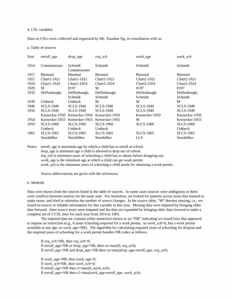
4. CSL variables

Data on CSLs were collected and organized by Ms. Xuanhui Ng, in consultation with us.

a. Table of sources

Year enroll_age drop_age req_sch work_age work_sch 1914 Commissioner Schmidt Schmidt Schmidt Schmidt

Commissioner1917 Biennial Biennial Biennial Biennial Biennial1921 Chart1-1921 Chart1-1921 Chart1-1921 Chart2-1921 Chart2-19211924 Chart1-1924 Chart1-1924 Chart1-1924 Chart2-1924 Chart2-19241929 M #197 M #197 #1971935 Deffenbaugh; Deffenbaugh; Deffenbaugh; Deffenbaugh; Deffenbaugh;

Schmidt Schmidt Schmidt Schmidt1939 Umbeck Umbeck M M M1946 SCLS-1946 SCLS-1946 SCLS-1946 SCLS-1946 SCLS-19461950 SCLS-1949 SCLS-1949 SCLS-1949 SCLS-1949 SCLS-1949

Keesecker-1950 Keesecker-1950 Keesecker-1950 Keesecker-1950 Keesecker-19501954 Keesecker-1955 Keesecker-1955 Keesecker-1955 M Keesecker-19551959 SCLS-1960 SLCS-1960 SLCS-1960 SLCS-1960 SLCS-1960

Umbeck Umbeck Umbeck Umbeck1965 SLCS-1965 SLCS-1965 SLCS-1965 SLCS-1965 SLCS-1965

Steinhilber Steinhilber Steinhilber LLS Steinhilber

Notes: enroll_age is maximum age by which a child has to enroll at school.drop_age is minimum age a child is allowed to drop out of school.req_sch is minimum years of schooling a child has to obtain before dropping out.work_age is the minimum age at which a child can get work permit.work_sch is the minimum years of schooling a child needs for obtaining a work permit.

Source abbreviations are given with the references.

b. Methods

Data were drawn from the sources listed in the table of sources. In some cases sources were ambiguous or therewere conflicts between sources for the same year. For resolution, we looked for patterns across years that seemed tomake sense, and tried to minimize the number of source changes. In the source table, “M” denotes missing, i.e., wefound no source or reliable information for this variable in this year. Missing data were imputed by bringing olderdata forward. Inter-source years were imputed and the data set expanded by bringing older data forward to make acomplete set of 5 CSL laws for each year from 1914 to 1965.

The imputed data set contains either numerical entries or an “NR” indicating we found laws that appearedto impose no restriction (e.g., 6 years schooling required for a work permit, so work_sch=6, but a work permitavailable at any age, so work_age=NR). The algorithm for calculating required years of schooling for dropout andthe required years of schooling for a work permit handles NR codes as follows:

If req_sch=NR, then req_sch=0;If enroll_age=NR or drop_age=NR, then ca=max(0, req_sch);If enroll_age£NR and drop_age£NR then ca=max(drop_age-enroll_age, req_sch).

If work_age=NR, then work_age=0;If work_sch=NR, then work_sch=0;If enroll_age=NR then cl=max(0, work_sch);If enroll_age£NR then cl=max(work_age-enroll_age, work_sch).

We coded a general literacy requirement without a specific grade or age requirement as NR. We coded a graderequirement of “elementary school” as 6, even though this was distinct from sixth grade in some sources (ourdummies would group these requirements anyway).

5. References for Appendix B

[Deffenbaugh] Deffenbaugh, Walter S. and Keesecker, Ward, W., Compulsory School Attendance Laws and TheirAdministration, US Department of Interior, Office of Education, Bulletin 1935, No. 4, Washington: USGPO (1935).

[Keesecker-1950] Keesecker, Ward, W. and Allen, Alfred, C., Compulsory School Attendance and MinimumEducational Requirements in the United States, 1950, Federal Security Agency, Office of Education,Circular No. 278 (September 1950).

[Keesecker-1955] Keesecker, Ward, W. and Allen, Alfred, C., Compulsory School Attendance and MinimumEducational Requirements in the United States, US Department of Health, Education, and Welfare, Officeof Education, Circular No. 440, Washington: US Department of Health, Education and Welfare (March1955).

[Schmidt] Schmidt, Stefanie, R., School Quality, Compulsory Education Laws, and the Growth of American HighSchool Attendance, 1915-35, MIT Ph.D. dissertation (1996).

[Steinhilber] Steinhilber, A.W. and Sokolowski, C.J., State Law on Compulsory Attendance, US Department of Health,Education and Welfare, Office of Education, Circular 793, Washington: US GPO (1966).

[Umbeck] Umbeck, Nelda, State Legislation on School Attendance and Related Matters - School Census and ChildLabor, US Department of Health, Education and Welfare, Office of Education, Circular No. 615, Washington:US GPO (January 1960).

[Biennial] US Department of the Interior, Bureau of Education, Biennial Survey of Education 1916-18. Bulletin 1919,No. 90 (1921).

[Commissioner] US Department of the Interior, Office of Education, Report of the Commissioner of Education forthe Year Ended June 30, 1917, Vol. 2, p. 69, Washington: US GPO.

[LLS] U.S. Department of Labor, Bureau of Labor Standards, Summary of State Child Labor Laws, Labor Law SeriesNo. 3-A, Washington: US Department of Labor (September 1966).

[SCLS-1946] U.S. Department of Labor, Division of Labor Standards, State Child-Labor Standards: A State-by-StateSummary of Laws Affecting the Employment of Minors Under 18 Years Of Age, Child Labor Series No. 2,Washington: US GPO (July 1946).

[SCLS-1949] _____, State Child-Labor Standards: A State-by-State Summary of Laws Affecting the Employment ofMinors Under 18 Years of Age, Bulletin 114, Washington: US GPO (September 1949).

[SCLS-1960] _____, State Child-Labor Standards: A State-by-State Summary of Laws Affecting the Employment ofMinors Under 18 Years of Age, Bulletin 158 (Revised 1960), Washington: US GPO (May 1960).

[SCLS-1965] _____, State Child-Labor Standards: A State-by-State Summary of Laws Affecting the Employment ofMinors Under 18 Years of Age, Bulletin 158 (Revised 1965), Washington: US GPO (September 1965).

[Chart1-1921] US Department of Labor, Children’s Bureau, State Child-Labor Standards, January 1, 1921," ChartSeries No. 1, Washington: US GPO.

[Chart1-1924] _____, State Child-Labor Standards, January 1, 1924, Chart Series No. 1, Washington: US GPO.[Chart2-1921] _____, State Compulsory School Attendance Standards Affecting the Employment of Minors, January

1, 1921, Chart Series No. 2, Washington: US GPO.[Chart2-1924] _____, “State Compulsory School Attendance Standards affecting the employment of minors, January

1, 1924," Chart Series No. 2, Washington: US GPO.[#197] _____ Child Labor Facts and Figures (October 1929) Bulletin 197, Washington: US GPO.

Table 1Descriptive Statistics for Census IPUMS

QOB SamplesVariables 1950 1960 1970 1980 1990

Covariates

Age 44.16(2.87)

44.55(2.88)

44.74(2.90)

44.66(2.94)

44.10(2.84)

Individual Education 9.67(3.40)

10.52(3.22)

11.59(3.18)

12.62(2.98)

13.70(2.49)

Regressors

State Average Education 9.94(0.72)

10.65(0.54)

11.52(0.41)

12.46(0.30)

13.10(0.23)

Lowest State AverageEducation

7.87[MS]

9.24[MS]

10.45[SC]

11.81[KY]

12.62[AR]

Highest State AverageEducation

11.18[UT]

11.80[UT]

12.38[UT]

13.07[DC]

13.74[DC]

Dependent Variable

Log Weekly Wage 4.06(0.77)

4.64(0.63)

5.17(0.65)

5.90(0.72)

6.44(0.73)

Instruments

Percent Child Labor 6 0.45 0.23 0.19 0.05 0.03

Percent Child Labor 7 0.45 0.36 0.24 0.24 0.16

Percent Child Labor 8 0.10 0.36 0.50 0.41 0.37

Percent Child Labor 9+ 0.01 0.05 0.07 0.31 0.44

Percent CompulsoryAttendance 8

0.57 0.35 0.24 0.11 0.11

Percent CompulsoryAttendance 9

0.40 0.53 0.44 0.44 0.44

Percent CompulsoryAttendance 10

0.02 0.06 0.08 0.09 0.06

Percent CompulsoryAttendance 11+

0.01 0.07 0.24 0.37 0.39

N 16659 72344 161029 376479 103184

Notes: Standard deviations are in parentheses. Bracketed entries in the ‘Lowest State Average Education’ and ‘HighestState Average Education’ rows are abbreviations indicating the state with the lowest and highest average schooling. Allother entries are means. The data are from the Census IPUMS for 1960 through 1980, with the sample restricted towhite males aged 40-49 in the Census year.

Table 2OLS Estimates of Private and Social Returns to Schooling

1960-1980

(1)

1950-1980

(2)

1950-1990

(3)

1950

(4)

1960

(5)

1970

(6)

1980

(7)

1990

(8)

A. Private Returns

Private Returnto Schooling

0.073(0.0003)

0.068(0.0003)

0.075(0.0003)

0.055(0.002)

0.069(0.001)

0.076(0.001)

0.075(0.001)

0.102(0.001)

State ofResidence

Main Effects?YES YES YES NO NO NO NO NO

B. Private and Social Returns

Private Returnto Schooling

0.073(0.000)

0.068(0.000)

0.074(0.000)

0.055(0.002)

0.068(0.001)

0.075(0.001)

0.074(0.000)

0.102(0.001)

Social Returnto Schooling

0.073(0.016)

0.061(0.004)

0.072(0.003)

0.136(0.017)

0.136(0.016)

0.128(0.021)

0.160(0.027)

0.168(0.047)

State ofResidence

Main Effects?YES YES YES NO NO NO NO NO

N 609852 626511 729695 16659 72344 161029 376479 103184

Notes: Standard errors corrected for state-year clustering are shown in parentheses. The data are from the CensusIPUMS for 1950 through 1990, with the sample restricted to white males aged 40-49 in the Census year. All regressionscontain Census year, year of birth, and state of birth main effects.

Table 3Description of Child Labor and Compulsory Schooling Laws

Year at Age 14(Census Year)

EarliestDrop Out

Age

(1)

LatestEnrollment

Age

(2)

MinimumSchooling

for Dropout

(3)

EarliestWork Age

(4)

RequiredSchoolingfor Work

Permit(5)

1914 (50) 15.31(1.20)

7.49(0.52)

1.90(3.40)

11.00(5.75)

1.70(2.56)

1917 (50) 15.55(0.89)

7.63(0.49)

1.93(2.74)

13.43(1.98)

2.98(2.66)

1921 (50) 15.69(0.99)

7.42(0.51)

4.28(3.63)

13.94(1.71)

4.19(2.97)

1924 (60) 15.88(0.97)

7.29(0.57)

5.64(3.64)

14.11(1.33)

4.91(3.04)

1929 (60) 15.97(0.93)

7.30(0.58)

5.66(3.62)

14.16(1.33)

5.31(3.01)

1935 (70) 15.96(0.94)

7.24(0.55)

7.24(3.73)

14.14(0.76)

6.02(2.67)

1939 (70) 16.16(1.05)

7.16(0.51)

7.29(3.74)

14.15(0.77)

6.01(2.70)

1946 (80) 16.31(0.63)

7.09(0.53)

7.91(4.00)

14.77(1.16)

4.67(3.37)

1950 (80) 16.27(0.60)

7.08(0.53)

7.94(4.49)

15.03(1.14)

3.51(3.47)

1954 (80) 16.30(0.63)

7.05(0.52)

7.79(4.65)

15.02(1.20)

4.06(3.67)

1959 (90) 16.25(0.60)

7.05(0.53)

7.40(4.79)

15.19(1.19)

3.49(3.56)

1964 (90) 16.20(0.60)

7.05(0.54)

7.44(4.79)

15.17(1.22)

3.51(3.57)

Notes: Standard deviations are in parentheses. All other entries are means. The data are from the Census IPUMS for1950 through 1990, with the sample restricted to white men aged 40-49 in the Census year. See the data appendix forsources and method.

Table 4aThe Effect of Compulsory Attendance Laws and Child Labor Laws on Individual Schooling

Including State of Residence Controls Without State of Residence Controls

1960-1980

(1)

1950-1980

(2)

1950-1990

(3)

1980

(4)

1960-1980

(5)

1950-1980

(6)

1950-1990

(7)

1980

(8)

Child Labor Laws

CL 7 0.095(0.030)

0.117(0.024)

0.173(0.021)

0.050(0.041)

0.105(0.077)

0.115(0.051)

0.175(0.043)

0.062(0.041)

CL 8 0.124(0.034)

0.130(0.032)

0.213(0.026)

0.132(0.034)

0.120(0.093)

0.119(0.075)

0.202(0.059)

0.143(0.034)

CL 9 0.259(0.039)

0.220(0.038)

0.398(0.028)

0.167(0.041)

0.269(0.098)

0.225(0.084)

0.410(0.059)

0.182(0.041)

Compulsory Attendance Laws

CA 9 0.117(0.027)

0.083(0.025)

0.189(0.020)

-0.011(0.034)

0.103(0.072)

0.068(0.057)

0.171(0.043)

-0.009(0.034)

CA 10 0.095(0.034)

0.059(0.036)

0.113(0.020)

0.100(0.044)

0.106(0.085)

0.074(0.077)

0.133(0.063)

0.104(0.045)

CA 11 0.167(0.038)

0.144(0.036)

0.260(0.028)

0.115(0.037)

0.184(0.103)

0.165(0.085)

0.290(0.063)

0.119(0.038)

N 609852 626511 729695 376479 609852 626511 729695 376479

Notes: Standard errors corrected for state-year clustering are shown in parentheses. The data are from the CensusIPUMS for 1950 through 1990, with the sample restricted to white males aged 40-49 in the Census year. All regressionscontain Census year, year of birth, and state of birth main effects.

Table 4bEffects of Child Labor and Compulsory Schooling Laws on Discrete Levels of Schooling

Results for 1960-1980 Results for 1950-1980

Completed 8Years orHigher

(1)

Completed10 Years or

Higher

(2)

Completed12 Years or

Higher

(3)

Completed14 Years or

Higher

(4)

Completed16 Years or

Higher

(5)

Completed 8Years orHigher

(6)

Completed10 Years or

Higher

(7)

Completed12 Years or

Higher

(8)

Completed14 Years or

Higher

(9)

Completed16 Years or

Higher

(10)

Dependent VariableMean

0.908 0.747 0.617 0.249 0.167 0.884 0.695 0.562 0.226 0.151

Child Labor Laws

CL 7 0.019(0.004)

0.019(0.005)

0.014(0.005)

-0.005(0.006)

-0.005(0.004)

0.031(0.004)

0.014(0.004)

0.009(0.003)

-0.004(0.004)

-0.004(0.003)

CL 8 0.032(0.005)

0.023(0.005)

0.018(0.005)

-0.014(0.007)

-0.014(0.046)

0.033(0.005)

0.019(0.005)

0.016(0.005)

-0.009(0.006)

-0.010(0.003)

CL 9 0.061(0.005)

0.045(0.006)

0.035(0.006)

-0.019(0.007)

-0.018(0.052)

0.065(0.005)

0.034(0.006)

0.024(0.006)

-0.021(0.007)

-0.007(0.004)

Compulsory Attendance Laws

CA 9 0.036(0.004)

0.014(0.004)

0.010(0.004)

-0.009(0.005)

-0.011(0.004)

0.032(0.004)

0.010(0.004)

0.006(0.004)

-0.010(0.005)

-0.010(0.003)

CA 10 0.020(0.004)

0.023(0.005)

0.025(0.005)

-0.011(0.006)

-0.008(0.005)

0.016(0.005)

0.022(0.005)

0.022(0.005)

-0.011(0.006)

-0.009(0.005)

CA 11 0.030(0.005)

0.034(0.006)

0.037(0.006)

-0.013(0.007)

-0.009(0.005)

0.022(0.005)

0.032(0.006)

0.032(0.005)

-0.010(0.007)

-0.005(0.005)

Notes: Standard errors corrected for state-year clustering are shown in parentheses. All entries are OLS estimates from a regression of a dummy for having completedthe indicated year of schooling on child labor law or compulsory attendance law dummies. All regressions also contain Census year, year of birth, state of birth, andstate of residence main effects. The data are from the Census IPUMS for 1950 through 1980, with the sample restricted to white males aged 40-49 in the Census year.The sample size for the 1960-1980 columns is 609,852; the sample size for the 1950-1980 columns is 626,511.

Table 52SLS Estimates of Private Returns to Schooling

CSL InstrumentsQOB Instruments CL Instruments CA Instruments

1960-1980

(1)

1980

(2)

1960-1970

(3)

1960-1980

(4)

1950-1980

(5)

1950-1990

(6)

1960-1980

(7)

1950-1980

(8)

1950-1990

(9)

Including State ofResidence Main

Effects

0.073(0.012)

0.090(0.016)

0.063(0.017)

0.076(0.034)

0.103(0.038)

0.113(0.018)

0.092(0.044)

0.099(0.052)

0.081(0.023)

No State of ResidenceMain Effects

0.073(0.012)

0.088(0.016)

0.063(0.017)

0.080(0.064)

0.112(0.060)

0.126(0.027)

0.101(0.088)

0.094(0.086)

0.100(0.040)

N 609852 376479 233373 609852 626511 729695 609852 626511 729695

Notes: Standard errors corrected for state-year clustering are in parentheses. All entries are two-stage least squares estimates of private returns to schooling,using the excluded instruments indicated above and discussed in the text. The data are from the Census IPUMS for 1950 through 1990, with the samplerestricted to white males aged 40-49 in the Census year. ‘QOB’ refers to the set 30 dummies interacting quarter of birth and year of birth. . ‘CL’ refers to a set ofdummies indicating state and year specific child labor laws. ‘CA’ refers to a set of dummies indicating state and year specific compulsory attendance laws. Allmodels contain Census year, year of birth, and state of birth main effects.

Table 62SLS Estimates of Private and Social Returns to Schooling

Individual Schooling Endogenous Individual Schooling Exogenous(1) (2) (3) (4) (5) (6) (7) (8)

Second-Stage Estimates

Instrument Set QOB& CL

QOB& CA

QOB,CA & CL

QOB,CA & CL,

Interactions

CL CA CL& CA

QOB,CA & CL,interactions

Private Returnto Schooling

0.074(0.012)

0.074(0.012)

0.075(0.012)

0.060(0.013)

0.073(0.0003)

0.073(0.0003)

0.073(0.0003)

0.073(0.0003)

Social Returnto Schooling

0.003(0.040)

0.017(0.043)

0.004(0.035)

0.005(0.033)

0.002(0.038)

0.018(0.042)

0.006(0.033)

-0.011(0.030)

First-Stage for State-Year Average Schooling

CL 7 0.080(0.028)

0.062(0.025)

0.084(0.028)

0.062(0.025)

CL 8 0.107(0.035)

0.068(0.031)

0.107(0.035)

0.068(0.031)

CL 9 0.227(0.036)

0.184(0.034)

0.226(0.035)

0.183(0.034)

CA 9 0.128(0.026)

0.102(0.023)

0.128(0.026)

0.104(0.030)

CA 10 0.122(0.030)

0.104(0.029)

0.122(0.030)

0.104(0.029)

CA 11 0.144(0.038)

0.094(0.036)

0.143(0.038)

0.094(0.036)

Notes: Standard errors corrected for state-year clustering are reported in parentheses. All entries are two-stage least squares estimates of returns to schooling,using the excluded instruments indicated above and discussed in the text. ‘QOB’ refers to a set of dummies interacting quarter of birth and year of birth.‘CL’ refers to a set of dummies indicating state and year specific child labor laws. ‘CA’ refers to a set of dummies indicating state and year specificcompulsory attendance laws. The data are from the Census IPUMS for 1960 through 1980, with the sample restricted to white males aged 40-49 in theCensus year. All regressions contain Census year, year of birth, state of birth, and state of residence main effects. The sample size for all columns is 609852.

Table 72SLS Estimates of Social Returns to Schooling: Additional Results

Individual Education Endogenous 1960-1980 Individual Education ExogenousBaseline

1960-1980

(1)

1960 & 1980Only

(2)

1970 & 1980Only

(3)

PrivateReturns

Separate byCensus

(4)

Private ReturnsSeparate byCensus and

State(5)

PrivateReturns=.08

(6)

PrivateReturns=.09

(7)

A. Results Using Child Labor Laws as Instruments

Social Returnto Schooling

0.003(0.040)

-0.006(0.036)

0.013(0.052)

0.007(0.039)

-0.024(0.039)

-0.006(0.038)

-0.018(0.039)

First Stage for State-Year Average Schooling

CL 7 0.080(0.028)

0.140(0.041)

0.057(0.032)

0.083(0.028)

0.080(0.026)

0.084(0.028)

0.084(0.029)

CL 8 0.107(0.035)

0.164(0.044)

0.074(0.034)

0.104(0.034)

0.100(0.031)

0.107(0.035)

0.107(0.035)

CL 9 0.227(0.036)

0.311(0.046)

0.154(0.033)

0.223(0.035)

0.210(0.032)

0.227(0.036)

0.227(0.035)

B. Results Using Compulsory Attendance Laws as Instruments

Social Returnto Schooling

0.017(0.043)

0.055(0.035)

0.047(0.049)

0.021(0.043)

-0.018(0.043)

0.011(0.042)

0.010(0.043)

First-Stage for State-Year Average Schooling

CA 9 0.128(0.026)

0.223(0.040)

0.090(0.018)

0.125(0.026)

0.118(0.023)

0.128(0.026)

0.128(0.026)

CA10 0.122(0.030)

0.260(0.048)

0.108(0.023)

0.120(0.030)

0.112(0.027)

0.122(0.030)

0.122(0.030)

CA 11 0.144(0.038)

0.239(0.051)

0.142(0.031)

0.141(0.037)

0.134(0.034)

0.143(0.038)

0.143(0.038)

C. OLS Estimates

Social Returnto Schooling

0.073(.0003)

0.081(0.015)

0.011(0.027)

0.079(0.017)

0.044(0.016)

0.069(0.017)

0.063(0.017)

N 609852 448823 537508 609852 969877 609852 609852

Notes: Standard errors corrected for state-year clustering are reported in parentheses. All entries are estimates of returns toschooling, using dummies for child labor laws or compulsory attendance laws as excluded instruments. The data are from theCensus IPUMS. Unless otherwise indicated, the sample is restricted to white males aged 40-49 in the Census year. Allregressions contain individual education, Census year, year of birth, state of birth, and state of residence main effects.

Table 82SLS Estimates of Private and Social Returns to Schooling: Additional Samples, Individual Education Treated As Exogenous

Baseline Results Separate Private Returns byCensus

Separate Private Returns byCensus and State

50-80(1)

50-90(2)

50-80(3)

50-90(4)

50-80(5)

50-90(6)

A. Results Using Child Labor Laws as Instruments

SocialReturn

0.009(0.025)

0.048(0.019)

0.023(0.025)

0.074(0.019)

-0.034(0.025)

0.041(0.021)

First-Stage for State-Year Average Schooling

CL 7 0.173(0.024)

0.165(0.019)

0.170(0.023)

0.162(0.019)

0.158(0.020)

0.145(0.016)

CL 8 0.126(0.036)

0.144(0.027)

0.123(0.035)

0.139(0.027)

0.113(0.031)

0.121(0.022)

CL 9 0.278(0.039)

0.333(0.026)

0.275(0.039)

0.327(0.026)

0.250(0.034)

0.280(0.022)

B. Results Using Compulsory Attendance Laws as Instruments

SocialReturn

0.040(0.038)

0.0006(0.027)

0.053(0.039)

0.038(0.027)

0.017(0.038)

-0.008(0.029)

First- Stage for State-Year Average Schooling

CA 9 0.133(0.028)

0.172(0.019)

0.130(0.027)

0.168(0.019)

0.118(0.023)

0.143(0.015)

CA 10 0.106(0.037)

0.167(0.028)

0.105(0.036)

0.164(0.027)

0.096(0.031)

0.139(0.022)

CA 11 0.096(0.042)

0.182(0.029)

0.095(0.041)

0.178(0.028)

0.087(0.036)

0.154(0.023)

C. OLS Estimates

SocialReturn

0.061(0.009)

0.072(0.006)

0.076(0.009)

0.094(0.007)

0.039(0.008)

0.057(0.004)

N 626510 729695 626510 729695 626510 729695

Notes: Standard errors corrected for state-year clustering are reported in parentheses. Estimates of social returns toschooling use dummies for child labor and compulsory attendance laws as excluded instruments. Individual schooling istreated as exogenous. The sample is restricted to white males aged 40-49 in the Census year. All regressions containindividual schooling, Census year, year of birth, state of birth, and state of residence main effects.

Table 9Estimates of Social Return to Schooling and Changes in Private Returned to Schooling

OLS

(1)

CL

(2)

CA

(3)

CA & CL

(4)

A. 1960-1980

Social Return toSchooling

0.053(0.016)

-0.029(0.038)

-0.015(0.043)

-0.012(0.032)

Interaction term -0.021(0.002)

0.029(0.009)

0.015(0.009)

0.011(0.007)

B. 1950-1980

Social Return toSchooling

0.034(0.009)

0.020(0.025)

0.065(0.038)

0.031(0.022)

Interaction term -0.015(0.001)

0.017(0.006)

0.006(0.008)

0.005(0.005)

Notes: Standard errors corrected for state-year clustering are in parentheses. In Panel A, the interaction term is parameterized as(Individual Education-11)*(State-Year Average Education-11), and in Panel B, it is parameterized as High School GraduateDummy*(State-Year Average Education-11), so the estimates of individual and average schooling main effects are evaluated at11 years of individual and average schooling. Excluded instruments in Panel A are individual schooling interacted with CL andCA dummies. Excluded instruments in Panel B are a high school graduate dummy interacted with CL and CA dummies. Allregressions contain Census year, year of birth, state of birth, and state of residence main effects.