NBER WORKING PAPER SERIES

REPORTED INCOMES AND MARGINAL TAX RATES, 1960-2000:EVIDENCE AND POLICY IMPLICATIONS

Emmanuel Saez

Working Paper 10273http://www.nber.org/papers/w10273

NATIONAL BUREAU OF ECONOMIC RESEARCH1050 Massachusetts Avenue

Cambridge, MA 02138January 2004

I am very grateful to Dan Feenberg for his help using the micro tax return data and the TAXSIM calculator.I thank Alan Auerbach, Gerald Auten, Robert Carroll, Dan Feenberg, Martin Feldstein,Wojciech Kopczuk,Andrew Leigh, Thomas Piketty, James Poterba, and especially Joel Slemrod for very helpful comments anddiscussions. Financial support from the Sloan Foundation and NSF Grant SES-0134946 is gratefullyacknowledged. The views expressed herein are those of the authors and not necessarily those of the NationalBureau of Economic Research.

©2004 by Emmanuel Saez. All rights reserved. Short sections of text, not to exceed two paragraphs, maybe quoted without explicit permission provided that full credit, including © notice, is given to the source.

Reported Incomes and Marginal Tax Rates, 1960-2000: Evidence and Policy ImplicationsEmmanuel SaezNBER Working Paper No. 10273January 2004JEL No. H3

ABSTRACT

This paper use income tax return data from 1960 to 2000 to analyze the link between reported

incomes and marginal tax rates. Only the top 1% incomes show evidence of behavioral responses

to taxation. The data displays striking heterogeneity in the size of responses to tax changes overtime,

with no response either short-term or long-term for the very large Kennedy top rate cuts in the

early1960s, and striking evidence of responses, at least in the short-term, to the tax changes since

the 1980s. The 1980s tax cuts generated a surge in business income reported by high income

individual taxpayers due to a shift away from the corporate sector, and the disappearance of business

losses for tax avoidance. The Tax Reform Act of 1986 and the recent 1993 tax increase generated

large short-term responses of wages and salaries reported by top income earners, most likely due to

re-timing in compensation to take advantage of the tax changes. However, it is unlikely that the

extraordinary trend upward of the shares of total wages accruing to top wage income earners, which

started in the 1970s and accelerated in the 1980s and especially the late 1990s, can be explained

solely by the evolution of marginal tax rates.

Emmanuel SaezUniversity of California549 Evans Hall #3880Berkeley, CA 94720and NBERsaez@econ.berkeley.edu

1 Introduction

Over the last 40 years, the U.S. federal income has undergone very large changes. Perhaps the

most striking change has been the dramatic decrease in top marginal income tax rates. From

1950 to the early 1960s, the statutory top marginal income tax rate was 91%. This top rate was

reduced to 70% by the Kennedy tax cuts in the mid 1960s. During the Reagan administrations

of the 1980s, the top tax rate was further reduced to 50% in 1982 by the Economic and Recovery

Tax Act (ERTA) of 1981, and down to 28% in 1988 by the Tax Reform Act (TRA) of 1986. The

top tax rate was then increased to 31% in 1991, and further to 39.6% in 1993 by the Omnibus

Budget Reconciliation Act (OBRA) of 1993. The top rate has been changed by the 2001 tax

reform, it is currently 38.6% (year 2003) and is scheduled to decline to 35% by 2006. While

only about five hundred taxpayers were subject to the top marginal tax rate of 91% in the early

1960s, by 2000, more than half a million taxpayers are subject to the top rate.1 Thus, the

continuous and drastic progressivity of the federal income tax system up to the very highest

income taxpayers has been replaced by a much flatter tax structure where an upper middle class

family can face the same marginal tax rate as the highest income earners in the United States.

In addition to the redistributive effects, the dramatic reductions in top tax rates might

have generated large behavioral responses: the net-of-tax value of an additional dollar of pre-

tax income (excluding state and local taxes) for those in the highest bracket has experienced

enormous variations over the period, from less than 10 cents in the early 1960s to more than

70 cents by the late 1980s, and around 60 cents by 2000. It is plausible to think that such

variations might have had substantial effects on the economic activity of high-income earners

such as labor supply decisions, career choices, and savings decisions, as well as on the form of

compensation (salary versus untaxed fringe benefits for example). Indeed, the intellectual weight

behind the dramatic reduction in marginal tax rates in the 1980s was the logic of supply side

economics arguing that lower tax rates could generate important increases in economic activity,

and perhaps even tax revenues. As documented by Feenberg and Poterba (1993, 2000) and

Piketty and Saez (2003), there has indeed been an extraordinary increase in the share of total

income accruing to upper groups in the income distribution over the last 25 years. For example,1The statistics on the number of taxpayers in each tax bracket have been reported in the Internal Revenue

Service (IRS) annual publication Statistics of Income regularly since 1961.

2

the income share of the top 1% taxpayers (excluding capital gains from the analysis), has surged

from less than 8% in the early 1970s to almost 17% in 2000 (Piketty and Saez, 2003). Feenberg

and Poterba (1993) pointed out that the timing of the increase in top income shares, and most

notably the surge in top income from 1986 to 1988 around TRA of 1986, appears to be closely

related to the cuts in top tax rates. Slemrod and Bakija (2000) and Piketty and Saez (2003)

note, however, that the surge in top incomes accelerated in the late 1990s, although top income

tax rates increased substantially in 1993.

The goal of the present paper is to understand the effects of marginal income tax rates

on reported incomes by analyzing the shares and composition of incomes accruing to various

groups in the top tail of the income distribution, and the marginal income tax rates faced by

those groups. The analysis will focus on the 1960-2000 period because this period spans all the

important tax changes since World War II,2 and allows us to use the large and stratified public-

use tax return micro-files released by the IRS since 1960 as well as the TAXSIM tax calculator

created and maintained by the NBER to estimate marginal and average tax rates.3

There is a large literature trying to estimate the effects of taxes on such decisions as labor

supply, savings, and retirement decisions. Over the past decade, a new literature has emerged

which has pointed out that these standard behavioral responses are only components of what

drives reported incomes; other responses such as the form of compensation, tax-deductible ac-

tivities, unmeasured effort, and compliance also ultimately determine reported incomes, and

these may be more elastic with respect to taxation. Feldstein (1999) shows that, under certain

conditions, it is the overall elasticity of taxable income with respect to the net-of-tax rate (one

minus the marginal tax rate) that is relevant for assessing the implications of tax changes for

revenue raising and welfare. The influential studies of Lindsey (1987) and Feldstein (1995),

examining the 1980s tax cuts, estimated very large elasticities, in excess of one. This striking

conclusion has generated a substantial body of work on this central elasticity parameter and

generated a wide range of estimated elasticities, ranging from Feldstein and Lindsey’s estimates

at the high end to close to zero at the low end,4 depending on the estimation methodology and2There are few studies on behavioral responses to taxation in the United States in the pre-war era. Goolsbee

(1999) provides a simple analysis of the most important episodes.3See Feenberg and Coutts (1993) for a description of the TAXSIM calculator.4See Gruber and Saez (2002) for a survey.

3

the tax reforms considered.

It is important to note that, in contrast to most previous studies, our analysis focuses on

reported incomes before deductions such as adjustments to gross income, personal exemptions,

standard and itemized deductions. Therefore, our income concept is market income rather than

taxable income. As taxable income is a smaller base than gross income and as some components

of deductions such as charitable giving or mortgage interest deductions are also responsive to

marginal tax rates, the elasticities of taxable income are likely to be larger than the elasticities

of reported incomes that we analyze here.5.

Our analysis shows that only the reported incomes of taxpayers within the top 1% of the

income distribution appear to be responsive to changes in tax rates over the 1960-2000 period.

Even upper middle income class taxpayers (within the top decile but below the top 1%), which

experienced substantial changes in marginal tax rates, show no evidence of responses to taxation,

either in the short-run or the long-run. Attributing all the gains of the top 1% relative to the

average to the changes in tax rates produces very large elasticities of income with respect to

net-of-tax rates, in excess of one. However, allowing for simple secular and non-tax related time

trends in the top income share reduces the elasticity drastically (to about 0.5). Top income

shares within the top 1% show striking evidence of large and immediate responses to the tax

cuts of the 1980s, and the size of those responses is largest for the very top income groups. In

contrast, top incomes display no evidence of short or long-term response to the extremely large

changes in the net-of-tax rates following the Kennedy tax cuts in the early 1960s.

Data on the composition of income show that part of the response to the 1980s tax cuts has

been due to a sudden and permanent shift of corporate income toward the individual income

sector using partnerships and subchapter S corporations, legal entities taxed only at the individ-

ual level. However, most of the surge in top incomes since the 1970s has been due to a smooth

and extraordinary increase in the wages and salary component (which includes stock-option

exercises). This wage income surge started slowly in the early 1970s and has accelerated over5Gruber and Saez (2002) find indeed larger elasticities for taxable income than for Adjusted Gross Income.

We focus on gross income because the nature and size of deductions has changed considerably over time so

that, in contrast to gross income, it is not possible to construct consistent time series of “taxable income”. An

extensive literature has analyzed the response of the main components of itemized deductions such as charitable

contributions and interest deductions.

4

the period, and especially during the last decade, and does not seem to be closely related to the

timing of the tax cuts. There is evidence of short-term responses of the wage income component

around TRA 1986 and OBRA 1993: top wages shares spike just after the tax reduction of 1986

and just before the tax increase of 1993, suggesting that highly paid employees were able to

re-time their compensation to take advantage of the tax changes. It is, however, very difficult to

tell apart a long term effect of tax cuts from a non-tax related secular widening of the disparity

of earnings.

The paper proceeds as follows. Section 2 describes the key identification issues in estimating

behavioral elasticities of income with respect to marginal tax rates and shows how such elasticity

estimates can be used for tax policy analysis. Section 3 presents the results on income shares

and marginal tax rates, as well as the evolution of the composition of top incomes. Section 4

concludes by contrasting the U.S. experience with evidence from other countries.

2 Conceptual Framework and Methodology

2.1 Estimating Elasticities

The economic model underlying the estimation of behavioral responses to income taxation is

a simple extension of the static labor supply model. Individuals maximize a utility function

u(c, z) increasing in after tax income c (available for example for consumption) and decreasing

in before tax income z (earning income is costly for example). The budget constraint takes

the form c = (1 − τ)z + R where τ is the marginal tax rate and R is virtual income. Such

maximization generates an individual “reported income” function z(1− τ,R) which depends on

the net-of-tax rate 1− τ and virtual income R.6 Each individual has a particular income supply

function reflecting his skills, taste for labor, etc. Income effects are assumed away so that the

income function z is independent of R and depends only on the net-of-tax rate.7 The key point

is that, in contrast to the standard labor supply model, not only changes in hours of work can6This reported income supply function remains valid in the case of non-linear tax schedules, c = (1− τ)z + R

then represents the linearized budget constraint at the utility maximizing point.7Labor supply studies in general estimate modest income effects (see Blundell and Pencavel, 1999 for a survey).

Gruber and Saez (2002) try to estimate both income and substitution effects in the case of reported incomes, and

find very small and insignificant income effects.

5

affect earnings z but also intensity of work on the job, career choices, form of compensation,

tax-deductible activities, etc. The analysis below will show that it is indeed the full response of

reported incomes that is relevant for tax policy (a point made by Feldstein, 1999).

The literature on behavioral responses to taxation has attempted to use tax reforms to

identify the elasticity of reported incomes with respect to the net-of-tax rate defined as, e =

[(1−τ)/z]∂z/∂(1−τ) in the notation used above. In order to isolate the effects of the net-of-tax

rate, one would want to compare observed reported incomes after the tax rate change to the

incomes that would have been reported had the tax change not taken place. Obviously, the

latter are not observed and must be estimated. The simplest method consists in using as proxy

reported incomes before the reform and hence relate changes in reported incomes before and

after the reform to changes in tax rates.

Lindsey (1987) and Feldstein (1995) applied this methodology to the ERTA 1981 and TRA

1986 tax changes and found that top income groups, which experienced the largest marginal tax

cuts, also experienced the largest gains in reported incomes. As a result, Lindsey (1987) and

Feldstein (1995) obtain very large elasticities, between 1 and 3, with preferred estimates around

1.5. There are several important issues with those estimates.

First, as pointed out by Slemrod (1996,1998) and Goolsbee (2000b), those elasticities will

be upward biased if, for non-tax related reasons, top incomes were increasing more rapidly than

average incomes during that period. A large body of work has suggested that non-tax factors,

such as skill biased technical progress, the development of international trade, or the decline of

unions might have lead to a substantial increase in earnings disparity in the 1980s (see Katz

and Autor, 1999 for a survey). To overcome this issue, it would be preferable to compare

taxpayers with similar incomes rather than comparing high incomes to middle incomes. In the

case of income taxation, this is difficult for two reasons. First, for most reforms, taxpayers with

similar incomes face very similar tax changes.8 Second, although the discontinuity in marginal

tax rates due to the progressive bracket structure creates sharp changes in marginal incentives

for taxpayers with very similar incomes,9 this cannot be satisfactorily exploited to estimate8In contrast, redistributive programs such as the Earned Income Tax Credit which is targeted to taxpayers

with children, allows to use taxpayers with no children but similar income as a plausibly better control group to

identify the effects of the program (see, e.g., Eissa and Liebman, 1996).9Saez (2003) tries to exploit this feature and the ‘bracket creep’ from 1979 to 1981 to identify behavioral

6

elasticities because it appears that taxpayers either control imperfectly their incomes or are

not well aware of the details of the tax code and their precise location on the tax schedule.10

Therefore, it is conceivable that only large or salient tax changes are likely to generate behavioral

responses, raising some interesting and complicated issues about the estimation of behavioral

responses and the design of tax policy (see Liebman and Zeckhauser (2003) for an analysis along

those lines).

Second, comparing years just before and just after the reform might reveal a short-term elas-

ticity, which can be quite different from the long-term elasticity, which is the relevant parameter

for tax policy. Slemrod (1995) discusses this point and Goolsbee (2000a) shows convincingly

that executives exercised massively stock options in 1992 in order to avoid the higher tax rate

starting in 1993, creating a large short-term elasticity of reported income around OBRA 1993;

the longer term elasticity was much smaller and possibly equal to zero.11 Looking at times series

spanning a number of years before and after the reform, as in Poterba and Feenberg (1993),

can be helpful to make progress on those two issues. Slemrod (1996) proposes an aggregate

time-series regression framework, for the period 1954 to 1990, to try and disentangle tax and

non-tax influences on the share and composition of income accruing to the top .5% taxpayers.

Third, the Lindsey and Feldstein studies assume implicitly that reported income elasticities

are the same for all income groups and, as we will see, the data strongly suggests that those

taxpayers with very high incomes are much more responsive to taxation than taxpayers in the

middle or upper middle class. More precisely, instead of adopting the simple difference method

just described, they compare changes in the incomes of the very high incomes (experiencing the

largest tax rate changes), to changes in incomes of the middle and upper middle class (experi-

encing more modest tax changes). This difference-in-differences of (log) incomes is then divided

by the corresponding difference-in-differences of (log) net-of-tax rates to obtain an elasticity

responses.10Saez (2002) documents in detail the fact that we do not observe bunching, as predicted by theory, at the kink

points of the tax schedule.11Feldstein and Feenberg (1996) noted a decrease in top reported incomes from 1992 to 1993 and interpreted this

finding as evidence of large behavioral elasticities. As compensation of executives continued to soar throughout

the late 1990s, negative long-run elasticity estimates would be obtained by repeating Goolsbee’s analysis and

comparing incomes in 1992 to those of the late 1990s.

7

estimate of the form:

e =∆ log(zH)−∆ log(zM )

∆ log(1− τH)−∆ log(1− τM )

where zH , zM and τH , τM denote the incomes and marginal tax rates of the high (H) and

middle (M) income groups respectively; and ∆ denotes the changes from before to after the tax

change. But suppose that the middle class has a zero elasticity so that ∆ log(zM ) = 0 and that

high income individuals have an elasticity of e so that ∆ log(zH) = e∆ log(1 − τH). Assume

further that the middle class experiences an increase in its net-of-tax rates that is half as large

as that experienced by the high income taxpayers so that ∆ log(1− τM ) = 0.5 ·∆ log(1− τH).

Then, the estimated elasticity e will be twice the true elasticity e of the high income group, a

dramatic upward bias in the estimate. This simple but realistic example shows that it is not

appropriate to rely on comparisons of the responsiveness of the reported incomes of the middle

and upper income groups when there is a strong suspicion that the behavioral elasticities for the

two groups are quite different.

Fourth, the increases in top incomes following the 1980s tax changes might have been due

in part to income shifting rather than creation of new income. As we show below, the critical

distinction for policy and welfare analysis, is whether the increase in reported incomes comes at

the expense of untaxed activities (such as leisure, fringe benefits, perquisites) or taxed activities

(such as profits in the corporate sector, future capital gains, deferred compensation such as

pensions). Slemrod (1996) points out that part of the surge in top incomes following TRA 1986

was due to a dramatic increase in S-corporation income, suggesting that many business owners

switched the legal form of their corporations from subchapter C (facing the corporate income

tax on their profits) toward subchapter S (which do not face the corporate tax and whose profits

are taxed directly at the individual level) as the top individual income tax rate became lower

than the corporate income tax rate by 1988.12 Carroll and Joulfaian (1997) explore this issue12A C-corporation faces the corporate tax on its profits. Profits are then taxed again at the individual level

if paid out as dividends. If profits are retained in the corporation, they may generate capital gains that are

taxed at the individual level but in general more favorably than dividends, when they are realized. Profits from

S-corporations (or partnerships and sole proprietorships) are taxed directly and solely at the individual level.

Distributions from S-corporations to individual owners generate no additional tax. Thus, a S-corporation is

fiscally more advantageous than the C-corporation the lower the individual tax rate, the higher the corporate tax

8

in more detail using a panel of corporations from 1985 to 1990, and confirm Slemrod’s (1996)

earlier findings. Gordon and Slemrod (2000) perform a systematic study of income shifting by

analyzing simultaneously tax changes and reported incomes at the corporate and personal level.

In this paper, we analyze in detail the composition of reported individual incomes in order to

cast light on the source of the changes in reported incomes following tax reforms.

The early studies by Lindsey (1987) and Feenberg and Poterba (1993) used the large and

stratified annual cross-sectional public-use tax return data to document the evolution of top

reported incomes. Following Feldstein (1995) influential analysis of the TRA 1986, a number

of studies have used panel data to estimate elasticities. The main justification put forward for

using panel data instead of repeated cross-sections is that it might alleviate the issue of non-tax

related changes in income inequality, as the same individuals are followed from before to after the

reform. However, it is plausible to think that an increase in income inequality might be in large

part due to high income individuals experiencing larger gains than lower income individuals,

in which case a panel analysis does not solve the issue. Furthermore, a tax cut might induce

middle incomes to try harder to become rich, and this behavioral response will be missed by a

Feldstein type panel data analysis.

The use of panel data has two additional important drawbacks. First, the publicly available

panel of tax returns is not stratified, and hence does not allow nearly as precise a study of

the evolution of top incomes as the large stratified cross-sections.13 Second, comparing groups

ranked according to pre-reform incomes generates a mean reversion problem: if there is mobility

in incomes from year to year, then it can cause high income taxpayers in one year to appear low

income in the next, aside from any true behavioral response.14 Eliminating this mobility bias

requires to control for pre-reform income in the estimation but this will weaken and possibly

destroy identification as the size of net-of-tax rates changes is closely correlated with income.15

rate, and the higher the capital gains tax rate (see Scholes (1992), Chapter 4, for extensive details and examples).

A business can switch to and from the C and S status but S-corporations cannot have more than a limited number

of stock-holders (75 currently), issue more than one class of stock, or be a subsidiary of other corporations.13Auten and Carroll (1999) have used a larger panel available only at the Treasury to compare years 1985 and

1989. It is, however, difficult to create longer panels to analyze longer term time series because of attrition issues.14This would generate a downward bias in the elasticity estimates in the case of a tax rate decrease such as

TRA 1986 and an upward bias in the case of a tax rate increase such as OBRA 1993.15This point is discussed in Gruber and Saez (2002) who overcome this problem by using many years instead

9

Many authors, including Lindsey (1987) himself, have argued that comparing income groups

using repeated cross-sections is a valid strategy only if taxpayers stay in the same groups from

year to year. However, following a tax rate cut such as ERTA 1981 or TRA 1986, one would

like to know how the distribution of reported income has changed relative to a scenario where

the tax change does not take place. Whether or not there is mobility in incomes from year to

year is independent of this question, as long as the income distribution is stationary (absent

the tax change). In contrast, mobility in incomes is precisely what complicates the panel data

analysis. Panel data, however, have key advantages to study some questions more subtle than

the overall response of reported incomes. For example, if one wants to study how a tax change

affects income mobility (for example, do more middle incomes becomes successful entrepreneurs

following a tax rate cut?), panel data is clearly necessary.

Measuring the tax induced change in the income distribution is exactly what is needed

to derive the tax revenue consequences of the tax change. Because we do not observe the

counterfactual income distribution when no tax change takes place, we have to rely on income

distributions from previous years, and there is no systematic bias in the repeated cross-section

analysis as long as the income distribution remains stationary, absent the tax change. The direct

focus on the income distribution series over-time allows a much more concrete and simple grasp

on the evolution of incomes for different groups than panel analysis, as it is straightforward

to divide the population into various percentiles for each year, and analyze simultaneously the

evolution of the incomes and the marginal tax rates of these groups. By relating the changes in

incomes to the changes in net-of-tax rates, we can obtain elasticity estimates.

Finally, Slemrod (1998) and Slemrod and Kopczuk (2002) make the important point that

the elasticity of reported incomes with respect to tax rates might not be a fixed parameter and

depends on the legal details and the enforcement of the tax system: for example, if it is easy

for corporations to switch from subchapter C to subchapter S to avoid taxes, the individual tax

base might be much more elastic than in a setting where subchapter S corporations do not exist.

Kopczuk (2003) performs an empirical analysis of this issue for the United States from 1979 to

1990, and shows that taxable income elasticities are negatively related to the base of incomes

of just two in the analysis. The implicit assumption they need to make, however, is that mobility remains stable

from year to year.

10

subject to taxes. This results suggests that introducing additional deductions increases the

responsiveness of taxable incomes. Goolsbee (1999) studies the key tax changes in the United

States since the 1920s and finds enormous heterogeneity in the observed responses from episode

to episode, although he does not try to explain the discrepancies. The present analysis of the

period 1960-2000 also displays significant heterogeneity in responses over time.

2.2 Using Elasticities for Tax Policy

The empirical analysis that follows will show that evidence of behavioral responses to changes

in marginal tax rates is concentrated in the top of the income distribution, with little evidence

of any response for the middle and upper-middle income class.16 Therefore, it is useful to focus

on the analysis of the effects of increasing the marginal tax rate on the upper end of the income

distribution. Let us therefore assume that incomes in the top bracket, above a given threshold

z, face a constant marginal tax rate τ .17 We denote by N the number of taxpayers in the top

bracket.

We assume that incomes reported in the top bracket depend on the net-of-tax rate 1 − τ ,

and we denote by z(1 − τ) the average income reported by taxpayers in the top bracket. As

discussed above, we assume away income effects in the analysis and thus the net-of-tax rate

is the only relevant parameter. The elasticity (compensated or uncompensated, as there are

no income effects) of income in the top bracket with respect to the net-of-tax rate is therefore

defined as e = [(1− τ)/z]∂z/∂(1− τ). Suppose that the government increases the top tax rate

τ by a small amount dτ (with no change in the tax schedule for incomes below z). This small

tax reform has two effects on tax revenue. First, there is a mechanical increase in tax revenue

due to the fact that taxpayers face a higher tax rate on their incomes above z. Hence, the total

mechanical effect is16The low end of the income distribution is out of the scope of the present paper because many low income

families and individuals do not file income tax returns. The large literature on responses to welfare and in-

come transfer programs targeted toward low incomes has, however, displayed evidence of significant labor supply

responses (see e.g., Meyer and Rosenbaum, 2001 for a recent analysis).17In the case of year 2003 tax law, for example, taxable incomes above z = $311, 950, are taxed at the top

marginal tax rate of τ = 38.6%.

11

dM = N [z − z]dτ.

This mechanical effect is the projected increase in tax revenue, absent any behavioral response.

Second, the increase in the tax rate triggers a behavioral response which reduces the average

reported income in the top bracket by dz = −e · z · dτ/(1− τ) on average and hence produces a

loss in tax revenue equal to

dB = −N · e · z · τ

1− τdτ.

Summing the mechanical and the behavioral effect, we obtain the total change in tax revenue

due to the tax change:

dR = dM + dB = Ndτ(z − z) ·[1− e · z

z − z· τ

1− τ

].

Let us denote by a the ratio z/(z − z). Note that a ≥ 1 and that a = 1 when z = 0, that is,

when there is a single flat tax rate applying to all incomes. If the top tail of the distribution

is Pareto distributed,18 then the parameter a does not vary with z and is exactly equal to the

Pareto parameter. As the tails of actual income distributions are very well approximated by

Pareto distributions, it turns out that the coefficient a is extremely stable for z above $200,000.

Saez (2001) provides such an empirical analysis for 1992 and 1993 incomes using tax return

data. The parameter a measures the thinness of the top tail of the income the distribution:

the thicker the tail of the distribution, the larger is z relative to z, and hence the smaller a.

Feenberg and Poterba (1993) provide estimates of the Pareto parameter a from 1951 to 1990

for the distribution of AGI in the United States using income tax returns and show that a has

decreased from about 2.5 in the early 1970s to around 1.5 in the late 1980s.19

We can rewrite the effect of the small reform on tax revenue dR simply as:18A Pareto distribution has a density function of the form f(z) = C/z1+α where C and α are constant param-

eters. α is called the Pareto parameter.19Piketty and Saez (2003) provide estimates of thresholds z and average incomes z corresponding to various

fractiles within the top decile of the U.S. income distribution from 1913 to 2000, allowing a straightforward

estimation of the parameter a for any year and income threshold.

12

dR = dM

[1− τ

1− τ· e · a

]. (1)

Formula (1) is of central importance. It shows that the fraction of tax revenue lost through

behavioral responses – the second term in the square bracket expression – is a simple function

increasing in the tax rate τ , the elasticity e, and the Pareto parameter a. This expression is

also equal to the marginal deadweight burden created by the increase in the tax rate. More

precisely, because of the envelope theorem, the behavioral response creates no additional welfare

loss as the individual is maximizing utility, and thus the utility loss (in dollar terms) created by

the tax increase is exactly equal to the mechanical effect dM . However, tax revenue collected is

only dR = dM + dB with dB < 0. Thus −dB represents indeed the extra amount lost in utility

over and above the tax revenue collected dR. The marginal excess burden expressed in terms of

extra taxes collected is simply

−dB

dR=

e · a · τ1− τ − e · a · τ

. (2)

Those formulas are valid for any tax rate τ and income distribution, even if individuals

have heterogeneous utility functions and behavioral elasticities.20 as long as income effects are

assumed away. Thus, this formula should be preferred to the Harberger triangle approximations

which require small tax rates to be valid. The parameters τ and a are straightforward to obtain,

the elasticity parameter e is thus the central non-trivial parameter necessary to make use of

formulas (1) and (2). For example, in 2000, for the top .5% income cut-off (corresponding

approximately to the top 39.6% federal income tax bracket in that year), Piketty and Saez

(2003) estimate that a = 1.6. For an elasticity estimate e = 0.5, corresponding to the mid

to upper range of the estimates from the literature, the fraction of tax revenue lost through

behavioral responses (dB/dM), should the top tax rate be slightly increased, would be 52.5%,

more than half of the mechanical projected increase in tax revenue. In terms of marginal excess

burden, increasing tax revenue by $1 requires to create a utility loss of 1/(1− .525) = $2.11 for

taxpayers, and hence a marginal excess burden of $1.11 or 111% of the extra $1 tax collected.

Following the supply-side debates of the early 1980s, much attention has been focused on the

tax rate maximizing tax revenue, the so-called “Laffer rate”. The Laffer rate τ∗ maximizes tax20The elasticity e is the average (income weighted) of individual elasticities.

13

revenue, hence the bracketed expression in equation (1) is exactly zero when τ = τ∗. Rearranging

the equation, we obtain the following simple formula for the Laffer tax rate τ∗ for the top bracket:

τ∗ =1

1 + a · e. (3)

A top tax rate above the Laffer rate is a very inefficient situation because decreasing the tax

rate would both increase government revenue and the utility of high income taxpayers.21 At the

Laffer rate, the excess burden becomes infinite as raising more tax revenue becomes impossible.

Using our previous example with e = 0.5 and a = 1.6, the Laffer rate τ∗ would be 55.6%, not

much higher than the combined maximum federal, state, medicare, and sales tax rate. Note that

when z = 0, and the tax system has a single tax rate, the Laffer rate becomes the well-known

expression τ∗ = 1/(1 + e). As a ≥ 1, the flat rate maximizing tax revenue is always larger than

the Laffer rate for high incomes only. This is because increasing the top tax rate collects extra

taxes only on the portion of incomes above the bracket threshold z but produces a behavioral

response for high incomes as large as an across the board increase in marginal tax rates.

The analysis has assumed so far that the reduction in incomes due to the tax rate increase

has no other effect on tax revenue. This is a reasonable assumption if the reduction in incomes

is due to reduced labor supply (and hence an increase in untaxed leisure time), or due to a shift

from cash compensation toward untaxed fringe benefits or perquisites (more generous health

insurance, better offices, company cars, etc.). However, in many instances, the reduction in

reported incomes is due in part to a shift away from individual income toward other forms of

taxable income such as corporate income, or deferred compensation, that will be taxable to the

individual when paid out (see Slemrod, 1998). For example and we will come back to this later

on in detail, Slemrod (1996) and Gordon and Slemrod (2000) show convincingly that part of the

surge in top incomes after the Tax Reform Act of 1986 was due to a shift of income from the21In the case where the government has strong redistributive tastes and does not value the marginal consumption

of high income individuals relative to the average individual, the optimal income tax rate for high incomes is exactly

equal to the Laffer rate (3). In the general case where the government values the marginal consumption of high

incomes at 0 ≤ g < 1, the optimal tax rate for the high incomes is such that the bracketed expression in (1) is

equal to g. See Saez (2001) for a more detailed exposition following the classical optimal income tax theory of

Mirrlees (1971).

14

corporate sector toward the individual sector.

Let us therefore assume that the incomes that disappear from the individual income tax

base following the tax rate increase dτ are shifted to other bases taxed at rate t on average.

For example, if two thirds of the reduction in individual reported incomes is due to increased

leisure and one third is due to a shift toward the corporate sector, t would be one third of the

corporate tax rate, as leisure is untaxed. In that case, it is straightforward to show that formula

(1) becomes:

dR = dM

[1− τ − t

1− τ· e · a

]. (4)

The same envelope theorem logic applies for welfare analysis and the marginal deadweight burden

formula is also modified accordingly by replacing e · a · τ by e · a · (τ − t) in both numerator and

denominator of (2). The Laffer rate (3) becomes:

τ∗ =1 + t · a · e1 + a · e

. (5)

If we assume again that a = 1.6 and e = .5, but that incomes disappearing from the individual

base are taxed at t = 20% on average, the fraction of revenue lost due to behavioral responses

drops from 52.5% to 26%, and the marginal excess burden (expressed as a percentage of extra

taxes raised) decreases from 111% to 35%, if the initial top tax rate is τ = 39.6%. The Laffer

rate increases from 55.6% to 64.5%. This simple theoretical analysis shows therefore, that, in

addition to estimating the elasticity e, it is critical to analyze the source or destination of changes

in reported individual incomes.

2.3 Data and Methodology

We estimate the level and shares of total income accruing to various upper income groups using

the large cross-sectional individual tax return data annually released by the IRS since 1960.22

The data are a stratified sample of tax returns oversampled for high-income taxpayers, allowing

an extremely precise analysis of top reported incomes. The top income shares are estimated22There is no micro data for years 1961, 1963, and 1965.

15

based on the Piketty and Saez (2003) analysis.23 The unit of analysis is the tax unit defined

as a married couple living together (with dependents) or a single adult (with dependents), as

in the current tax law. It is important to keep in mind that top income shares series measured

at the tax unit level, as we do here, might be different from series estimated at the individual

level. As displayed in Table A, since 1960, the average number of individuals per tax unit has

decreased from 2.6 to 2.1 due to the decrease in the average number of dependent children per tax

unit as well as the decrease in the fraction of married tax units. Those long-term demographic

changes imply that real average income growth per tax unit will be substantially smaller than

real income growth per capita. These demographic changes can also affect top income shares

if the reduction in tax units size is not uniform across income groups. However, the tax return

data show that the reduction in tax unit size has been about the same for high incomes than

for the U.S. population as a whole. From 1960 to 2000, the number of individuals per tax unit

in the top decile has declined from 3.6 to 2.9, which is the same 20% decline as in the general

population (from 2.6 to 2.1).

From 1960 to 2000, the fraction of married tax units has declined from about 60% to 50% for

the population at large (due to the increased number of single parents and non married couples)

but only from 90% to 85% for the top decile tax units. An increase in single tax units with lower

incomes contributes to increasing top income shares. Similarly, an increase in the correlation

of earnings between spouses (due for example to increased labor force participation of married

women) would also increase top income shares estimated at the tax unit level. Those slow

moving demographic changes, however, are small relative to the dramatic trends we document

and can only explain at best a very small fraction of the changes in the very top income shares.

Each upper income group is defined relative to the total number of potential tax units in

the entire U.S. population, estimated from population and family census data as the sum of

married men, divorced and widowed men and women, and of single adults never married (aged

20 and above).24 The income definition we use is consistent over time and includes all income23The main (and very minor) difference is that government transfers such as Social Security benefits and

Unemployment Compensation have been excluded from the income definition in this paper in order to obtain

better consistency in the income definition over years. The estimates have been extended to year 2000.24From 1960 to 2000, between 90 and 95% of potential tax units actually filed an income tax return, as many

non-taxable families file in order to get tax refunds.

16

items excluding realized capital gains25 reported on tax returns and before all deductions such

as adjustments to gross income, exemptions, itemized and standard deductions. We exclude

government transfers such as Social Security (SS) benefits and Unemployment Insurance (UI)

benefits. Thus, our income measure is defined as Adjusted Gross Income (AGI) less realized

capital gains included in AGI, less taxable SS and UI benefits, plus all the adjustments to

gross income. Hence, our measure of income is a broader measure than taxable income on which

many previous studies have focused. If deductions to income such as charitable giving, mortgage

interest payments, etc. are also responsive to taxation, taxable income might be more responsive

to tax rates than our broader income measure. However, as the nature of deductions allowed

has changed substantially over the period 1960-2000, it is impossible to construct a consistent

taxable income definition over the full period. As a result, we refer the reader to previous studies

analyzing specifically the components of taxable income that we exclude from the analysis.

As in Piketty and Saez (2003), we consider various groups within the top decile of the income

distribution. In order to get a more concrete sense of those upper income groups, Table 1 displays

the thresholds, the average income level in each group, along with the number of tax units in

each group, all for 2000. The median income, as well as the average income for the bottom 90%

of tax units is quite low, around $25,000. Those numbers are smaller than those reported by

the Census Bureau based on the Current Population Survey (CPS) for two reasons. First, our

income definition does not include any government transfers. Second, CPS income is reported

at the household level which is a larger unit than the tax unit we consider.26

The groups in the top decile below the top 1% (the top 10-5% denotes the bottom half

of the top decile, and the top 5-1%, the next 4 percentiles) have average incomes of $100,000

and $160,000 respectively, which corresponds, perhaps surprisingly given how far up the income

distribution those groups are, to the popular view of the middle and upper middle income class.

In 2000, an annual family income of at least $280,000 is required to be part of the top 1%.

Hence, the top 1% corresponds perhaps to the popular view of the high incomes. About 140,000

tax units (or slightly more than 0.1% of all tax units) report incomes larger than one million25Realized capital gains are excluded because they form a very volatile component of income and face in general

a different tax treatment than other forms of income. There is a large literature focusing on the response of capital

gains realizations to tax changes. See Auerbach (1988) for a survey.26For example, a cohabiting couple or two roommates form a single household but two tax units.

17

dollars (the very high incomes). Finally, the top .01%, the smallest top group we consider, is

formed by the top 13,400 tax units, reporting on average $13 million of annual income in 2000,

these are the super high income American families.

We estimate shares of income by dividing the income amounts accruing to each group by re-

ported income, where we have assumed that non-filing units earn 20% of the average income.27

We then estimate the composition of income for each group and we consider seven compo-

nents: salaries and wages (including exercised stock-options, bonuses, and private pensions),

S-corporation income, sole proprietorship (Schedule C income) and farm income, partnership

income, dividends, interest income, and other income (including smaller item such as rents,

royalties, and other miscellaneous items).

Marginal tax rates are estimated using the TAXSIM tax calculator. For each individual

record, we compute a weighted marginal tax rate based on wage income and other income as

various provisions in the tax code generate differences in the tax treatment of wage income and

other forms of income. For each income group, we then estimate an average marginal tax rate

weighted by income.28 It is important to note that our marginal tax rate computations ignore

state income taxes because the data does not provide state information for high income earners.

Our tax measure also ignores other taxes such as social security and medicare taxes, corporate

taxes, and non-income taxes such as sales and excise taxes.

We use the same methodology to compute top wage shares using wages and salaries reported

on tax returns. Wages and salaries include exercised stock-options and bonuses. In this case,

groups are defined relative to the total number of tax units with positive wage income estimated

as the number of part-time and full workers from the National Income and Product Accounts less

the number of married women who are employees. The sum of total wages in the economy used

to compute shares is obtained from National Income and Product Accounts (total compensation

of employees). The marginal tax rates for upper wage income groups are of course those relevant

for wages and salaries and are also weighted by wage income (see Table A).

We propose a very simple time series regression methodology to obtain various elasticity

estimates, and illustrate some of the identification difficulties. Because of potential heterogene-27As only between 5 and 10% of tax units do not file returns, our results are not sensitive to this assumption.28As we saw above, for tax policy analysis, it is necessary to weight marginal tax rates by income.

18

ity in elasticities across income groups, all our regressions are run for a single income group.

The simplest specification consists in regressing log real incomes on log net-of-tax rates (and a

constant) for a given group. Of course, as real incomes grow over time, we can add time trends

in the regression to control for exogenous (i.e., non-tax related) real income growth. Those es-

timates are unbiased estimates of behavioral elasticities, if absent any tax change, real incomes

in that specific group do not change (first specification) or follow a regular time pattern (second

specification). These assumptions may not be met. As many years of data are included, these

estimates capture mostly the long-term behavioral elasticities.29 As we will see, the pattern of

average incomes for the full population does no appear to be related to the evolution of average

marginal tax rates, therefore, in order to control for average income growth, we run most of the

regressions in terms of log income shares instead of log average incomes.30 Those regressions

control automatically for overall income growth. Adding time trends in that case amounts to

assuming that incomes for the particular group considered may diverge from the average income

in the economy. As we are running time-series regressions and the error terms appear to be

correlated over time (according to the standard Durbin-Watson test), OLS standard errors are

not correct. Therefore, we compute the Newey-West standard errors assuming that the error

terms can be correlated up to an eight year lag.31

Due to the progressive structure of the income tax, increases in incomes lead to higher

marginal tax rates because of bracket-creep. As a result, an increase in top income shares (for

non-tax related reasons) might also induce a mechanical increase in the marginal tax rate faced

by those high incomes, hence potentially biasing downward our elasticity estimates. A simple

way to investigate the extent of the problem is to use the statutory top marginal income tax

rate (or more precisely the log of one minus the top rate) as an instrument for the effective log

net-of-tax rate variable. Our results show that the OLS and IV estimates are extremely close,

suggesting that this bracket-creep issue does not create a significant estimation problem.29We leave for future research the regression analysis of the dynamics of tax responses. Such a formal analysis

has been attempted in the case of capital gains realizations (see, e.g., Auerbach, 1988).30Slemrod (1996) adopted the same approach, although he controlled for non-tax factors explicitly rather than

using general time trends controls as we do here.31An eight year lag is close to maximizing the size of the standard errors, and thus should be seen as conservative.

19

3 Income Shares and Marginal Tax Rates

3.1 Trends in Average Incomes

We depict on Figure 1, the average federal marginal individual income tax rate (weighted by

income) and the average income (per tax unit) reported in real terms for the full population

from 1960 to 2000. Incomes are expressed in 2000 dollars using the standard CPI-U deflator

(see Table A). Figure 1 shows that real incomes increased quickly from 1960 to 1973 and then

hardly increased until the early 1990s. From 1993 to 2000, real incomes have increased quickly

but are only 13% higher than in 1973. Real growth depends critically on the CPI deflator.

Improvements in the CPI estimation have been made over the years and some of them have

been incorporated retrospectively in the so-called CPI-U-RS deflator (see Stewart and Reed,

1999). Using the CPI-U-RS instead of the CPI-U would display about 29% real income growth

instead of 13% from 1973 to 2000 (see Table A).

Average marginal tax rates display significant movements with a steady increase from 21-

22% to 30% from the mid 1960s to the early 1980s (with a temporary surge during the Vietnam

war surtaxes in 1968-70). In the 1980s, the average marginal tax rate decreased to 23%, and

increased slightly to 26% during the 1990s. Figure 1 displays no clear relation between the level

of real incomes and the level of marginal tax rates. As displayed in Table 2, Panel A, a simple

OLS regression of log average incomes on the log of the net-of-tax rate controlling or not for

time trends to account for exogenous economic growth, display insignificant elasticity coefficients.

Therefore, the aggregate data displays no evidence of significant behavioral responses of reported

incomes to changes in the average marginal tax rate.

Figure 2 shows a striking contrast between the bottom 99% tax units (Panel A) and the

top 1% (Panel B). The average real income of the bottom 99% increased steadily from 1960 to

1973 and then stagnated: real incomes in 2000 are hardly higher than in 1973.32 The decline in

marginal tax rates faced by the bottom 99% from almost 30% in 1981 to around 23% in 2000

does not seem to have noticeably improved the growth of real incomes. Indeed as shown in Table32If one uses the CPI-U-RS deflator, the bottom 99% real incomes would have grown by about 13%. In any

case, it is clear that real growth of incomes has been very slow in last quarter of the 20th century relative to the

1950-1973 period. It is also important to note that this slow growth is not due to a decrease in the number of

adults per tax units (see Table A).

20

2, Panel B, regressing the log average incomes on the log net-of-tax rate for the bottom 99%

displays negative (although insignificant) coefficients whether or not a time trend is included.

In stark contrast, the average real income of the top 1% has increased by 160% since the

early 1970s (or by 200% if one uses the CPI-U-RS), and the average marginal tax rate has also

declined substantially, from around 50% before 1981 to less than 30% by 1988. It is striking to

note that the top 1% incomes start increasing precisely in 1981 when marginal tax rates start

going down. The jump in top incomes from 1986 to 1988 corresponds exactly to the sharp drop

in marginal tax rates from 45% to 29% after the Tax Reform Act of 1986. These points, first

noted by Poterba and Feenberg (1993), suggest that high incomes are indeed quite responsive

to taxation. The other striking feature of the figure is the extraordinary increase in top incomes

from 1994-2000 in spite of the increase in tax rates from about 32% to almost 40% in 1993.

Thus, although the marginal tax rates faced by the high incomes in 2000 are hardly lower than

in the mid-1980s (39% instead of 44-45%), top incomes are more than twice larger.

Figure 2 illustrates very well the difficulty of obtaining convincing estimates of the elasticity

of reported income with respect to the net-of-tax rate. It seems clear that the sharp, and

unprecedented, increase in incomes from 1986 to 1988 is related to the large decrease in marginal

tax rates that happened exactly during those years. The central question, however, is whether

this short-term response persists overtime. In particular, how should we interpret the continuing

rise in top incomes in since 1994? If one thinks that this surge is evidence of diverging trends

between high incomes and the rest of the population independent of tax policy, which started

in the 1970s, then it is tempting to consider the response of TRA 1986 as a purely short-term

spike followed by lower growth from 1988 to 1993, before getting back to the normal upward

trend by 1994. On the other hand, one could argue that the surge in top incomes since the

mid-1990s might have been the long-term consequence of the decrease in tax rates in the 1980s

and that such a surge would not have occurred, had high incomes tax rates remained high as in

the 1960s and 1970s. We come back to this point later on.

Those issues are illustrated formally in the regression results of Table 2, Panel C. When no

time trend is included in the regression of log income on log net-of-tax rate, all the growth in top

incomes is attributed to the decline in top rates, and the elasticity obtained is extremely large

1.83 (.37). In contrast, including a time trend produces a much smaller, although still sizeable,

21

elasticity .71 (.22) because part of the rise in top incomes is attributed to a secular rise. Adding

an additional time square control further reduces the elasticity to 0.5 (0.18).

This analysis also shows that, comparing two single years by taking the ratio of the difference

in log incomes to the difference in log net-of tax rates, as done in most studies, can produce a

wide range of elasticity estimates. Comparing 1981 to 1984, as in Lindsey (1987), would produce

an elasticity of 0.77.33 Comparing 1985 and 1988, as in Feldstein (1995) and Auten and Carroll

(1999), would produce an extremely large 1.7 elasticity.34 In contrast, comparing 1991 to 1994

(as in Goolsbee, 2000a) would produce a zero elasticity because top incomes are about constant

while tax rates increase by almost 10 percentage points.35 The elasticity would even become

negative if one compares 1991 to the late 1990s as both top incomes and the tax rate have

increased.36 The large micro-data sets can be used to obtain those simple elasticity estimates

directly from regressions at the individual level as done in many studies, with very small standard

errors. The regression counterpart would be to pool the samples of top 1% earners for the pre

and post reform years, and run a 2SLS regression of log incomes on log net-of-tax rate using

as an instrument a post year dummy.37 In order to cast further light on those issues and try

to separate tax effects from other effects, we turn to a closer analysis of various upper income

groups, with particular emphasis on the change in the composition of reported incomes.33Lindsey obtains larger estimates because he compares the upper income to the middle income groups, creating

an upward bias if, as is apparent in the data, elasticities are increasing with income (see discussion above).34Auten and Carroll (1999) obtain a much smaller 0.6 elasticity because they compare 1985 to 1989 (instead of

1988 as Feldstein) and because of the mean reversion issue discussed above which is difficult to correct with only

two years of data.35In contrast, comparing 1992 to 1993 would produce a significant short-term elasticity of 0.63 as in Feldstein

and Feenberg (1996).36Carroll (1998) and Sammartino and Wiener (1997) analyze panel tax return data also show that short term

responses around OBRA 1992 are much larger than longer term responses.37It is doubtful, however, that those small standard errors would be accurate, as random year effects are

most likely to be present in the data making 2SLS standard errors far too low and hence worthless (in addition

to creating the identification problems discussed above). See Bertrand, Duflo, and Mullainathan (2003) for a

detailed discussion of those econometric issues.

22

3.2 Trends in Top Income Shares and Marginal Tax Rates

We have shown that average real incomes do not seem to respond to average marginal tax rates

in the aggregate, and that responses seem to be concentrated in the upper 1% fraction of the

income distribution. Therefore, from now on, we normalize top incomes by considering the shares

of total income accruing to various upper groups (as in Feenberg and Poterba, 1993 and 2000,

and Piketty and Saez, 2003). This has two advantages. First, the income share measures are

independent of the CPI deflator used. Second, the top shares are automatically normalized for

overall real and nominal growth in incomes. All our top income share series and corresponding

average marginal tax rates (income weighted) are reported in Tables B1 and B2 respectively.

Table 3 displays a number of regressions of the (log) top 1% income share on the log net-of-tax

rate, varying the number of time trends controls and instrumenting or not the tax variable with

the log net-of-tax top rate. As discussed above, introducing time trends reduces substantially the

elasticity (from 1.6 with no controls) to about 0.6-0.7 (with many controls). After adding linear

and square controls in time, the adjusted R-square reaches 98% and the elasticity coefficient is

not sensitive to adding further controls. The IV estimates are very close in magnitude to the

OLS estimates and have a strong first stage (except in the case of col. (4) where the first stage is

weak), suggesting that the issue of reverse causality because of the progressive nature of the tax

schedule is not an important issue. Figure 3 illustrates those issues by plotting, along with the

top 1% income share series, the fitted values from the regressions with no time controls (dotted

line) and with two time controls (solid line). The dotted line shows that the pure tax effects

explain quite poorly the evolution of the top 1% income share. In contrast, the solid line with

two time trends captures extremely well the pattern of the top 1% income share (the adjusted

R-square of the regression is 98%). The dashed line in Figure 3 displays the counterfactual

pattern assuming that the marginal tax rate for the top 1% had remained constant since 1960.

This curve shows that most of growth in the top 1% income share is due to the time trends and

that only 2 out of the 9 percentage point increase in the top 1% income share from the 1960s

to 2000 is due to the decline in marginal tax rates. Therefore in summary, attributing all the

increase in the top income shares to the tax developments generate very large elasticities but fits

the data poorly. Controlling for time trends fits the data much better and reduces substantially

the elasticity as well as the fraction of the increase in top incomes that can be attributed to tax

23

changes.

Figure 4 displays the share of income accruing to the bottom half of the top decile (Panel A),

and the bottom half of the top percentile (Panel B), along with the average marginal tax rate

faced by those two groups. The figure shows that the top 10-5% income group has experienced

very moderate gains since 1960 and the pattern of the gains does not appear to be correlated

with the pattern of the marginal tax rates they face (rising up to 1981, then declining in the

1980s, and then stable in the 1990s). Panels A and B in Table 4 show that regressing the log

of the top income shares of the top 10-5% and top 5-1% on their log net-of-tax rates, with or

without time trend controls produces elasticities very close to zero. Therefore, upper middle

income families and individuals (up to the top 1% threshold around $280,000 per year in 2000)

do not appear to be sensitive to taxation.38 It is striking, in particular, that those upper middle

income class shares increase very little during the 1980s although they experience quite sizeable

marginal tax rate cuts (about 9 percentage points for the top 10-5%, and over 13 points for the

top 5-1%).39 Note again that IV estimates are also virtually identical to OLS estimates.

Interestingly, Panel B of Figure 4 shows that the top 1-.5% share does not decrease during

the 1970s when the marginal tax rate increases from 40 to 50% and does not increase during

ERTA 1981 when the marginal tax rate decreases back to 40%. In contrast, TRA 1986, which

decreases the rate to around 32% (thus a smaller percentage change in the net-of-tax rate relative

to the 1970s or ERTA 1981) does produce a sizeable increase in the income share, producing

a noticeable break in the series. The increase in tax rates to about 38% following OBRA 1992

does not seem to have affected the upward trend following TRA 1986. Thus although marginal

tax rates in the late 1990s are about the same as in the 1960s, the income share is 30% larger.40

38In principle, the secondary earner labor supply responses should be captured by those elasticities. Thus our

results can be consistent with the large married women labor supply responses obtained by Eissa (1995) only if

secondary earners income is a small fraction of total reported family incomes.39A similar regression analysis for other income groups below the top decile generates small or even negative and

always insignificant elasticities. The estimates, however, are not very precisely estimated as changes in net-of-tax

rates are much smaller below the top decile.40Those considerations show again that elasticity estimates would be extremely sensitive to the time period

considered. The ERTA 1981 and OBRA 1993 episodes would produce zero elasticity estimates, and TRA 1986

would produce a sizeable 0.93 estimate (comparing 1986 and 1988). Comparing 2000 to 1984 and attributing all

the large increase in the share to the modest decrease in marginal tax rate would produce an enormous elasticity

24

The regressions for the groups top 1-.5% and top .5-.1% in Table 4 (Panels C and D) display

significant elasticities but the size of the elasticity is much smaller when income controls are

included.

Figure 5 displays the share of income and marginal tax rates for the very top groups: top

.1-.01% (Panel A), and the top .01% (Panel B). The responses to ERTA 1981, TRA 1986, and

the short-term response to OBRA 1993 followed by a surge in income shares since 1995, are

even more pronounced than for the groups just below. However, the Kennedy tax cuts of the

early 1960s provide striking new evidence. For the very top .01%, the very progressive tax

structure of the early 1960s generated extremely high marginal tax rates (around 80%) which

were reduced significantly by the Kennedy tax cuts in 1964-5 (to about 65%).41 This implies a

75% increase in the net-of-tax rate, a much larger increase than the ERTA 1981 and TRA 1986

tax rate reductions. In spite of this enormous marginal tax rate cut, the very top share remains

flat in the 1960s, and well into the 1970s, suggesting a complete absence of behavioral response

in both the short and the long-run.42 Note that, although the top nominal marginal tax rate

was 91%, the average marginal tax rate of the top .01% is “only” slightly above 80%. This is due

to various other provisions of the tax code such as the maximum average tax of 87% on income

and charitable gifts by the very wealthy.43 Table 4 (Panels E and F) show that the regressions

for the top .1-.01% and the top .01% display significant elasticities is all specifications, although

pure tax factors can only explain a fraction of the total increase in the very top shares once

exogenous time trends are included.

estimate of 4.94.41Those tax cuts were proposed by president Kennedy in the early 1960s but were actually implemented by the

Johnson administration after Kennedy’s death in 1963.42Lindsey (1990) claimed that the Kennedy tax cuts generated a surge in top incomes, but this erroneous result

is due to his very casual examination of the tabulations published by the IRS. Goolsbee (1999) makes a more

careful use of the same published data (although he does not exclude realized capital gains and does not measure

marginal tax rates very accurately) and finds no response, as we do here.43Considering smaller groups at the very top, such as the top .001%, never generates marginal tax rates higher

than 80-82%.

25

3.3 Composition

We have seen in the previous subsection that the income groups within the top decile display very

heterogeneous responses. Groups below the top 1% never display evidence of tax responsiveness.

Top groups display a sharp response to the 1980s tax cuts, and especially TRA 1986, but only

a short-term response to the tax increase of 1993, and no response for the earlier tax cuts in

the 1960s. In order to cast further light on these findings, we now turn to an analysis of the

composition of those incomes.44 The complete composition series of top income groups are

reported in Tables D1 and D2 of the longer working paper version Saez (2004).

Figure 6 displays the evolution of the top decile income share, and how those incomes are

decomposed into the seven sources described in Section 2, from 1960 to 2000. Wage income

forms the majority of the top 10% incomes, and its share has increased smoothly from two

thirds to about three quarters since 1960. Interesting, the large 12 percentage point gain in the

top 10% income share (from 32% to 44%) is due almost entirely to a smooth and secular increase

in the wage component (from 22 points to 33.5 points), with the size of the other components

remaining stable overall (around 10 points with a squeeze around 7 points in the late 1970s and

early 1980s).

As depicted in Figure 7, the top 1% income share increases from 8.3% to almost 17% from

1960 to 2000. The striking feature, however, is that 7 out of the 8.7 point increase in the top

1% share is due to the wage income component. As a result, although wages represented only

40% of total income of the top 1% in the early 1960s, they now represent over 60% of top 1%

incomes. The increase in the wage component appears to have started in the early 1970s and

has been fairly regular with an acceleration in the last two decades (especially the 1990s). There

are two spikes in the wage component series, one in 1988 (just after TRA 1986), and another in

1992 (just before the OBRA 1993 tax increase). However, the short-term nature of those two

spikes suggests that they were the consequence of re-timing of wage income to take advantage

of lower rates.45

44The previous literature has mostly focused on taxable income elasticities. Feenberg and Poterba (1993,2000)

analyze the composition of incomes for the top .5% from 1951 to 1990 and Slemrod (1994,1996) analyze the

composition of top incomes around TRA 1986.45Goolsbee (2000a) showed that executives exercised massively their stock-options in 1992 in order to take

advantage of the low rate of 31% in 1992 before the increase to 39.6% in 1993. This retiming explains the large

26

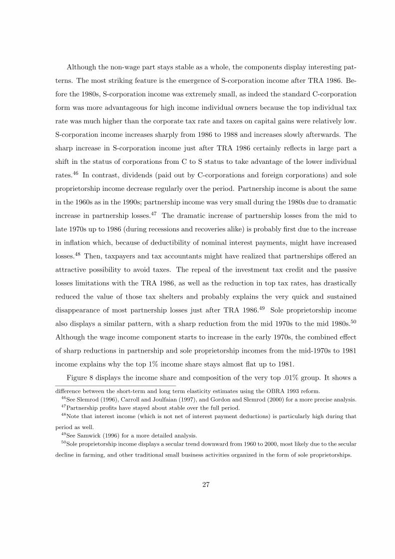
Although the non-wage part stays stable as a whole, the components display interesting pat-

terns. The most striking feature is the emergence of S-corporation income after TRA 1986. Be-

fore the 1980s, S-corporation income was extremely small, as indeed the standard C-corporation

form was more advantageous for high income individual owners because the top individual tax

rate was much higher than the corporate tax rate and taxes on capital gains were relatively low.

S-corporation income increases sharply from 1986 to 1988 and increases slowly afterwards. The

sharp increase in S-corporation income just after TRA 1986 certainly reflects in large part a

shift in the status of corporations from C to S status to take advantage of the lower individual

rates.46 In contrast, dividends (paid out by C-corporations and foreign corporations) and sole

proprietorship income decrease regularly over the period. Partnership income is about the same

in the 1960s as in the 1990s; partnership income was very small during the 1980s due to dramatic

increase in partnership losses.47 The dramatic increase of partnership losses from the mid to

late 1970s up to 1986 (during recessions and recoveries alike) is probably first due to the increase

in inflation which, because of deductibility of nominal interest payments, might have increased

losses.48 Then, taxpayers and tax accountants might have realized that partnerships offered an

attractive possibility to avoid taxes. The repeal of the investment tax credit and the passive

losses limitations with the TRA 1986, as well as the reduction in top tax rates, has drastically

reduced the value of those tax shelters and probably explains the very quick and sustained

disappearance of most partnership losses just after TRA 1986.49 Sole proprietorship income

also displays a similar pattern, with a sharp reduction from the mid 1970s to the mid 1980s.50

Although the wage income component starts to increase in the early 1970s, the combined effect

of sharp reductions in partnership and sole proprietorship incomes from the mid-1970s to 1981

income explains why the top 1% income share stays almost flat up to 1981.

Figure 8 displays the income share and composition of the very top .01% group. It shows a

difference between the short-term and long term elasticity estimates using the OBRA 1993 reform.46See Slemrod (1996), Carroll and Joulfaian (1997), and Gordon and Slemrod (2000) for a more precise analysis.47Partnership profits have stayed about stable over the full period.48Note that interest income (which is not net of interest payment deductions) is particularly high during that

period as well.49See Samwick (1996) for a more detailed analysis.50Sole proprietorship income displays a secular trend downward from 1960 to 2000, most likely due to the secular

decline in farming, and other traditional small business activities organized in the form of sole proprietorships.

27

dramatic shift in the composition of very top incomes away from dividends (which represented

more than 60% of top incomes in the early 1960s) toward wage income (which represents about

60% of top incomes in 2000).51 In the early 1960s, the top .01% incomes were facing extremely

high marginal tax rates of about 80% on average (while tax rates on long-term capital gains were

around 25%). Thus, dividends were a very disadvantaged form of income for the rich suggesting

that those top income earners had little control over the form of payment, and thus might have

been in large part passive investors. The Kennedy tax cuts did not reduce the top individual

rate enough (the top rate became 70%) to make the S-corporation form attractive relative

to the C-corporation form, explaining perhaps the contrast in behavioral responses between

the Kennedy tax cuts episodes and the tax changes of the 1980s. This shows, as argued by

Slemrod and Kopczuk (2002), that the elasticity of reported incomes is not a constant parameter

but may be extremely sensitive to the legal structure, and the complete tax environment for

corporations and individuals. The share of dividends falls regularly over the period while the

share of wage income starts to increase in 1971. By 1979, the wage component overtakes the

dividend component. Figure 8 shows clearly that ERTA 1981 produced a sudden burst of S-

corporation income (which was negligible up to 1981). This is most likely due to a shift from

C-corporations to S-corporations.52 It is interesting to note that the increase in S-corporation

income is concentrated mostly in the top .01% and does not happen at all for groups below the

top .1%. This is fully consistent with the tax minimization explanation: ERTA 1981 decreased

marginal tax rates significantly only for groups above the top .1% for whom the subchapter S

status started to become attractive when the top individual rate was reduced to 50%.53 Figure 8

shows that almost all the increase in top incomes from 1981 to 1984, first documented by Lindsey

(1987), is also due to the surge in S-corporation income. The wage component increases as well

but with no noticeable break in the upward trend around ERTA 1981.54 The S-corporation

component increases again sharply from 1986 to 1988, and then stay about stable afterwards.51This secular shift from rentiers to the working rich at the top of the U.S. income distribution is described in

more detail in Piketty and Saez (2003).52As discussed above, this phenomenon has been well documented in the case of TRA 1986.53From 1980 to 1986, the corporate tax rate was 42%.54Because of the maximum tax of 50% on labor income enacted in 1971-2, marginal tax rates for top wage

incomes actually did not change much with ERTA, see below.

28

The wage component also presents a spike in 1988, as well as in 1993, but those spikes seem to be

short-term responses in a generally upward trending curve. The tax cuts of the 1960s, although

extremely large, did not generate any behavioral response, perhaps because top individual rates

remained substantially higher than the corporate and capital gains tax rate and thus did not

induce top taxpayers to switch corporate income toward individual income.

Therefore, to sum up, the dramatic increase in top income shares is due primarily to a

secular increase in the wage income component starting in the early 1970s, and the large tax

changes of TRA 1986 and OBRA 1993 seem to have only generated short-term spikes in the

overall upward and accelerating trend of the wage component.55 The tax cuts of the 1980s

have generated a surge in business income taxed at the individual level. ERTA 1981 created a

surge in S-corporation income for the very top groups of the income distribution. With TRA

1986, S-corporation income surged for all upper income groups. Partnership income also rose

dramatically immediately after TRA 1986, mostly because of the disappearance of partnership

losses. Those business income components have remained relatively stable after TRA 1986,

suggesting that they were the consequence of a one-time shift from the corporate sector, and the

one-time closing of the partnership loss tax shelters. The top tax rate increase of 1993 to 39.6%

(with a corporate tax rate of 35%) was not large enough to induce business owners to switch back

to the C-corporation status. As a result, OBRA 1993 did not produce any long term income

shifting away from the individual sector and its only effect seem to have been a short-term

re-timing of salary income. The surge in business income reported on individual returns in the

1980s cannot be interpreted as a “supply-side” success as most of those individual income gains

came either at the expense of taxable corporate income, or could have been obtained from the

closing of tax-shelters by imposing stricter rules on losses from passive businesses.56 Therefore,

success or failure of the tax cuts to generate additional economic activity must be deferred to a55Top income shares are flat before 1981 masking the increase in the wage component, because of a large

decline in partnership and sole proprietorship income due perhaps to high interest rates and the development of

tax shelters in the 1970s. Partnership income (and to a lesser extent sole proprietorship income), increased back

to its early 1970s level immediately after TRA 1986.56It is doubtful that the decrease in tax rates, by reducing the incentives to avoid taxes, was necessary to

eliminate abusive partnership losses (as argued for example in Samwick, 1996) because partnership losses were

almost non-existent before the late 1970s, a time where tax rates were extremely high.

29

more precise analysis of the central wage income component, to which we now turn.

3.4 Top Wage Incomes

We have seen that most of the increase in top income shares since the 1970s is actually due to a

sharp increase in the wage income component. The time pattern of marginal tax rates for wage

income is not the same as the pattern for other forms of income because of the introduction of

the maximum tax rate on earned income in 1971 which reduced the top rate for earned income

from 70% (the top rate on other income) to 60% in 1971 and then 50% starting in 1972.57 This

provision became irrelevant in 1982 when the top tax rate for any income source was reduced

from 70% to 50%. Therefore, it is of particular interest to analyze separately the wage income

component. All our top wage income share series and corresponding average marginal tax rates

for wage income are reported in Tables C1 and C2 respectively.

As for average income, the evolution of average real wage income series (for the full pop-

ulation) does not appear to be correlated with the evolution of marginal tax rates. Figure 9

shows the pattern of real incomes and marginal tax rates for the bottom 99% wage earners

(Panel A) and the top 1% wage earners (Panel B). The bottom 99% experienced no real growth

in wage income since 1972, and the pattern of changes in real wages does not seem to be re-

lated to changes in marginal tax rates. In contrast, top 1% wage income earners experienced

accelerating growth over the 1960 to 2000 period, with almost a tripling in real wage income

since the early 1970s. Consistent with the pattern of the wage component for overall income,

top wage incomes experienced spikes just after TRA 1986 and just before OBRA 1993, clear

evidence of short-term responses (or re-timing) of labor income compensation. However, the

long-run pattern seems to be an extraordinary and accelerating growth independent of the tax

developments, as marginal tax rates on those wage income earners were about the same, around

40%, in the mid 1960s and in the most recent years. Indeed, the secular growth in top wages

starts in the early 1970s, a time when marginal tax rates were actually increasing (due mostly

to bracket creep). To understand better this unprecedented increase in top wage incomes, it is

useful to consider smaller groups within the top 1% as we did for overall income.57As described in Slemrod (1994), due to the interaction of this provision with the regular schedule, the marginal

income tax rate on labor income could be higher than those limits in a number of cases.

30

Table 5 produces the same regressions as Table 4 but for wage incomes instead of overall

income.58 The shares of the bottom groups of the top decile below the top 1% (top 10-5% and

top 5-1%) display very low elasticities, while all groups within the top 1% display significant

elasticities when no time trend is included, increasing sharply from 0.3 to 2.5 as we move up

the wage income distribution. This is because all the increase in the top wage income shares

is attributed to the secular decline in marginal tax rates since the 1960s. Including two time

trends reduces significantly the estimated elasticities which are below 0.4 except for the very top

groups. Even within the top 0.1%, where elasticities are sizeable, tax changes can only explain

a very small fraction of the dramatic surge in top wage incomes.

They key point to resolve is whether we should attribute the long-term increase in top wage

shares entirely to the long-term decrease in marginal tax rates. Comparing 1960 and 2000,

that seems to be an untenable view for groups below the top .1% because those groups faced

comparable marginal tax rates in 1960 and in 2000. As a result, the sizeable increase in the top

1-.5% and top .5-.1% wage income shares cannot be due entirely to marginal tax rates.

The problem is more complicated for the very top groups (within the top .1%) because those

groups experienced much larger gains but also experienced a non trivial decline in marginal tax

rates. Undoubtedly, a reason for the huge increase in top wage income shares (the top .01% share

increased more than ten-fold from .21% in 1970 to 2.45% in 2000) has been the development of

stock-options. Stock-options also create lumpiness in wage compensation as they are exercised

by executives only once every few years. As a result, the top .01% might be extremely large

in recent years because, in any given year, very top wage earners are executives who happen

to exercise their stock-options in that particular year. The stock-option phenomenon, however,

has clearly increased the average compensation of top executives as the top 1%, which certainly

includes virtually all the top employees receiving large option grants, even when they do not

exercise stock-options, more than doubles from 5.1% to 12.6% from 1970 to 2000.

Thus, the extraordinary increase in top wage incomes, a phenomenon certainly closely related

to the explosion of the compensation of CEOs and other top executives, sports, movies, and

television stars, appears too large to have been solely the direct consequence of the tax reductions58We have omitted the IV estimates in the case of wages because the first stage is not as strong as in the case

of income and the estimates are more noisy.

31

through supply-side effects. Furthermore, the surge in top wages is not related closely enough

to the timing of the tax cuts to suggest a direct and simple causal link. Particularly surprising

is the surge in top wages since 1994, in spite of the significant tax increase in 1993, which makes

the secular reduction in marginal tax rates faced by top wage groups appear rather small.59

A more pertinent question to ask is perhaps whether this surge in top wages could have

occurred, had the tax structure remained the same as in the early 1960s, and the working rich

had to pay in taxes more than three quarters of their compensation. It is plausible to think that

the drastic reduction in top marginal tax rates, which started in the 1960s, opened the possibility

of the dramatic increase in top wages that started in the 1970s, and accelerated in the 1980s

and the 1990s. It is of course impossible to provide a convincing answer to that important

question by looking only at individual income tax statistics in the United States. A promising

way to make progress would be look more closely into the top salaries surge phenomenon by

analyzing executive compensation data. There is a large literature on executive compensation

(see Murphy, 1999 for a survey). However, although there are many studies explaining disparity

of CEO pay in cross-sectional data, no convincing explanation for the time series evidence seems

to have been provided.60 If the dramatic surge in top compensation is not fully explained by a

comparable surge in the marginal productivity of top executives, then this is evidence of a market

failure which would certainly change the welfare and tax policy analysis that we presented above.

Alternatively, top executive pay may now be aligned to marginal product and was below market

value before. We note, however, that the surge in the top 1% salaries since the early 1970s has

been accompanied with a dismal growth for the bottom 99% salary earners, and thus does not

seem to have had a positive impact on the vast majority of working families. An alternative

way to make progress in our understanding is by looking at other countries experiences, a point

to which we now turn for our conclusion.59Companies, however, might have started granting stock-options more aggressively after TRA 1986 because

of the decrease in individual tax rates. Those options can be exercised (and thus appear on individual income

tax returns) only a number of years later. Hall and Murphy (2003) show, however, that grants of stock-options,

valued using the Black-Scholes formula, increased massively after the tax increase of 1993.60It is quite telling to read in the recent survey of Hall and Murphy (2003), two prominent and conservative

researchers in this field, that their best explanation for the surge in stock-option compensation was that “boards

and managers falsely perceive stock options to be inexpensive because of accounting and cash-flow considerations”.

32

4 Conclusion: International Comparisons

Unfortunately, no other country offers such a large body of empirical analysis on behavioral

responses to individual income taxation than the United States. Recently, however, a number of

studies have produced series of top income shares using tax return data. Although, those studies

do not produce corresponding series of marginal tax rates, as we have done here, interesting

findings emerge.

First, there is enormous heterogeneity in the behavior of top income shares in the recent

decades across countries. Some countries, such as the United Kingdom (Atkinson, 2002) or

Canada (Saez and Veall, 2003) have experienced notable increases in top income shares, although

those increases have not been as pronounced as in the United States. In contrast, countries from

continental Europe such as France (Piketty, 2001), the Netherlands (Atkinson and Salverda,

2003), or Switzerland (Dell, Piketty, and Saez, 2003) have experienced either declines or little

changes in top income shares since the 1960.

Second, the United Kingdom experience seems to be the closest to the U.S. experience.

Top income shares in the United Kingdom started increasing exactly in 1979 when the top

rate declined from 98% to 75%, although this increase seems modest relative to size of net-

of-tax increase at the top.61 In 1988, the top rate was further decreased to 40% and has not

changed since then. In contrast to the United States however, the increase in top share has been

relatively smooth since 1979 with no break around the tax changes. Studying the composition,

and estimating precisely the marginal tax rates faced by top U.K. incomes seems to be a priority

to understand whether the recent increase in top incomes is due to the tax developments.62

Third, Canada has experienced a surge in top incomes significantly larger than the United

Kingdom (although smaller than the United States), and as in the United States, this increase

has been due to a dramatic increase in top salaries since the early 1980s. However, in contrast

to the United States, top incomes in Canada have not experienced, very large tax cuts since the

1960s.63 Thus, the dramatic increase in top incomes in Canada cannot be attributed solely to61It might be the case, however, that for the top .1% incomes, the average decline in marginal tax rates has

been much more modest.62Dilnot and Kell (1988) try to analyze this issue but have only access to a single year of micro-tax returns and

have to rely on aggregate numbers for their time series analysis.63The top income tax rate in Canada, including provincial taxes, is about 50% in 2000.

33

fiscal developments in Canada. Saez and Veall (2003) argue that the threat of emigration toward

the United States have forced Canadian companies to increase the pay of their top employees to

retain them, thereby replicating in Canada the dramatic U.S. increase in top employees’ pay. If

the migration threat explanation is correct, it implies that the surge in top wage incomes in the

United States is a real phenomenon and not uniquely a consequence of repackaging of income

in order to avoid taxes.

Last, in contrast to the United States and the United Kingdom, France, Netherlands, and

Switzerland have experienced relatively small changes in their top tax rates. Piketty (1999)

shows that the small changes in the French top tax rates generated small short-term responses

of top incomes but that those responses do not seem to persist overtime. Switzerland has lower

top income tax rates than the United States (around 35% when adding federal, cantonal, and

local income taxes), but has much lower top income shares than the United States (the top 1%

share is around 8-9% in the 1990s, while it is between 13 and 17% in the United States).

In sum, high income tax rates do not seem to be able to account for the differences in

top income shares across countries, although it is more debatable whether they can account

for a substantial part of the time series pattern within countries. Therefore, it would be of

most interest to make a systematic analysis of top incomes in countries which have experienced

drastic cuts in top income tax rates in the recent decades, as in the United States and the

United Kingdom. Those results could teach us whether a dramatic cut in top rates is necessarily

associated with a rise in top incomes.

References

Atkinson, Anthony (2002). “Top Incomes in the United Kingdom over the Twentieth Century.”

mimeo Nuffield College, Oxford.

Atkinson, Anthony, and Wiemer Salverda (2003). “Top Incomes in the Netherlands and the

United Kingdom over the Twentieth Century.” mimeo Nuffield College, Oxford.

Auerbach, Alan (1988). “Capital Gains Taxation in the United States.” Brookings Papers on

Economic Activity 2, 595-631.

Auten, Gerald, and Robert Carroll (1999) “The Effect of Income Taxes on Household Behavior.”

Review of Economics and Statistics 81(4), 681-693.

34

Bertrand, Marianne, Esther Duflo, and Sendhil Mullainathan (2002). “How Much Should We

Trust Differences-in-Differences Estimates?”, NBER Working Paper No. 8841, forthcoming

Quarterly Journal of Economics.

Blundell, Richard, and Thomas MaCurdy (1999). “Labor supply: A Review of alternative

approaches.”. In O. Ashenfelter, D. Card (Eds.), Handbook of Labor Economics, Amsterdam:

North-Holland, Volume 3.

Carroll, Robert (1998). “Tax Rates, Taxpayer Behavior, and the 1993 Tax Act.” Office of Tax

Analysis working paper, U.S. Department of the Treasury.

Carroll, Robert, and David Joulfaian (1997). “Taxes and Corporate Choice of Organizational

Form.” Office of Tax Analysis Working Paper No. 73, U.S. Department of the Treasury.

Dell, Fabien, Thomas Piketty, and Emmanuel Saez (2003). “The Evolution of Income and

Wealth Concentration in Switzerland over the 20th Century.” mimeo UC Berkeley.

Dilnot, Andrew, and Michael Kell (1988). “Top-Rate Tax Cuts and Incentives: Some Empirical

Evidence.” Fiscal Studies 9, 70-92.

Eissa, Nada (1995). “Taxation and Labor Supply of Married Women: the Tax Reform Act of

1986 as a Natural Experiment.” NBER Working Paper No. 5023.

Eissa, Nada, and Jeffrey Liebman (1996). “Labor Supply Response to the Earned Income Tax

Credit.” Quarterly Journal of Economics, 111, 605-637.

Feenberg, Daniel, and Elisabeth Coutts (1993). “An introduction to the TAXSIM model.”

Journal of Policy Analysis and Management 12(1), 189-194.

Feenberg, Daniel, and James Poterba (1993). “Income Inequality and the Incomes of Very High

Income Taxpayers: Evidence from Tax Returns”, In Tax Policy and the Economy ed. J. Poterba,

(MIT Press: Cambridge), 7, 145-177.

Feenberg, Daniel, and James Poterba (2000). “The Income and Tax Share of Very High Income

Households, 1960-1995”, American Economic Review, 90(2), 264-270.

Feldstein, Martin (1995). “The Effect of Marginal Tax Rates on Taxable Income: A Panel Study

of the 1986 Tax Reform Act.” Journal of Political Economy 103(3), 551-572.

Feldstein, Martin (1999). “Tax Avoidance and the Deadweight Loss of the Income Tax”, Review

of Economics and Statistics 81(4), 674-680.

Feldstein, Martin, and Daniel Feenberg (1996). “The Effect of Increased Tax Rates on Taxable

35

Income and Economic Efficiency: A Preliminary Analysis of the 1993 Tax Rate Increases”, In

Tax Policy and the Economy ed. J. Poterba, (MIT Press: Cambridge), 10, 89-117.

Goolsbee, Austan (1999). “Evidence on the High-Income Laffer Curve from Six Decades of Tax

Reform.” Brookings Papers on Economic Activity 2, 1-47.

Goolsbee, Austan (2000a). “What Happens When You Tax the Rich? Evidence from executive

compensation.” Journal of Political Economy 108(2), 352-378.

Goolsbee, Austan (2000b). “It’s not about the Money: Why Natural Experiments Don’t Work

on the Rich.” In Slemrod J. (Ed.) Does Atlas Shrug? The Economic Consequences of Taxing

the Rich, Cambridge University Press.

Gordon, Roger, and Joel Slemrod (2000). “Are ‘Real’ Responses to Taxes Simply Income

Shifting Between Corporate and Personal Tax Bases?” In Slemrod J. (Ed.) Does Atlas Shrug?

The Economic Consequences of Taxing the Rich, Cambridge University Press.

Gruber, Jonathan, and Emmanuel Saez (2002). “The Elasticity of Taxable Income: Evidence

and Implications.” Journal of Public Economics 84, 1-32.

Hall, Brian, and Kevin Murphy (2003). “The Trouble with Stock Options”, NBER Working

Paper No. 9784.

Katz, Lawrence, and David Autor (1999). “Changes in the Wage Structure and Earnings In-

equality.” in Handbook of Labor Economics, eds. O. Ashenfelter and D. Card, Amsterdam:

North-Holland, Volume 3A.

Kopczuk, Wojciech (2003). “Tax Bases, Tax Rates and the Elasticity of Reported Income.”,

NBER Working Paper No. 10044.

Liebman, Jeffrey, and Richard Zeckhauser (2003). “Schmeduling”, Harvard University mimeo.

Lindsey, Lawrence (1987). “Individual Taxpayer Response to Tax Cuts: 1982-1984, with Impli-

cations for the Revenue Maximizing Tax Rate.” Journal of Public Economics 33, 173-206.

Lindsey, Lawrence (1990). The Growth Experiment: How the New Tax Policy is Transforming

the U.S. Economy (New York: Basic Books, Inc.)

Meyer, Bruce, and Daniel Rosenbaum (2001). “Welfare, the Earned Income Tax Credit, and

the Labor Supply of Single Mothers.” Quarterly Journal of Economics 116(3), 1063-1114.

Mirrlees, James A. (1971). “An Exploration in the Theory of Optimal Income Taxation.” Review

of Economic studies 38, 175-208.

36

Murphy, Kevin J. (1999). “Executive Compensation.” in Handbook of Labor Economics, eds.

O. Ashenfelter and D. Card, Amsterdam: North-Holland, Volume 3B.

Piketty, Thomas (1999). “Les Hauts Revenus face aux Modifications des Taux Marginaux

Superieurs de lImpot sur le Revenu en France, 1970-1996.” Economie et Prevision 138-139,

25-60.

Piketty, Thomas (2001). “Income Inequality in France, 1901-1998.” CEPR Discussion Paper

No. 2876, forthcoming Journal of Political Economy.

Piketty, Thomas, and Emmanuel Saez (2003). “Income Inequality in the United States, 1913-

1998.” Quarterly Journal of Economics 118(1), 1-39. Series updated to year 2000 at http://www.nber.org/papers/w8467

Saez, Emmanuel (2001). “Using Elasticities to Derive Optimal Income Tax Rates.” Review of

Economic Studies 68, 205-229.

Saez, Emmanuel (2002). “Do Taxpayers Bunch at Kink Points?” Mimeograph, University of

California at Berkeley.

Saez, Emmanuel (2003). “The Effect of Marginal Tax Rates on Income: A Panel Study of

‘Bracket Creep’.” Journal of Public Economics 87, 1231-1258.

Saez, Emmanuel (2004). “Reported Incomes and Marginal Tax Rates, 1960-2000: Evidence and

Policy Implications.” NBER Working Paper No. 10xxx.

Saez, Emmanuel, and Michael Veall (2003). “The Evolution of High Incomes in Canada, 1920-

2000.” NBER Working Paper No. 9607.

Sammartino, Frank, Weiner, David (1997). “Recent evidence on taxpayers’ response to the rate

increases in the 1990’s.” National Tax Journal 50(3), 683-705.

Samwick, Andrew (1996). “Tax Shelters and Passive Losses after the Tax Reform Act of 1986.”

In Empirical Foundations of Household Taxation, eds. M. Feldstein and J. Poterba, University

of Chicago.

Scholes, Myron and Mark A. Wolfson (1992). Taxes and Business Strategy: A Planning Ap-

proach, Prentice Hall.

Slemrod, Joel (1994). “On the High Income Laffer Curve.” in J. Slemrod (ed.) Tax Progressivity

and Income Inequality, Cambridge University Press: Cambridge, 177-210.

Slemrod, Joel (1995). “Income Creation or Income Shifting? Behavioral Responses to the Tax

Reform Act of 1986.” American Economic Review, 85(2), 175-180.

37

Slemrod, Joel (1996). “High Income Families and the Tax Changes of the 1980s: the Anatomy

of Behavioral Response.” In Empirical Foundations of Household Taxation, eds. M. Feldstein

and J. Poterba, University of Chicago.

Slemrod, Joel (1998). “Methodological issues in Measuring and Interpreting Taxable Income

Elasticities.” National Tax Journal 51(4), 773-788.

Slemrod, Joel, and Jonathan Bakija (2001). “Growing Inequality and Decreased Tax Progres-

sivity.” in K. Hassett (Ed.) Inequality and Tax Policy, Washington D.C: American Enterprise

Institute Press.

Slemrod, Joel, and Wojciech Kopczuk (2002). “The Optimal Elasticity of Taxable Income.”

Journal of Public Economics 84(1), 91-112.

Stewart, Kenneth J., and Stephen B. Reed (1999). “CPI Research Series Using Current Methods,

1978-98.” Monthly Labor Review, June.

U.S. Treasury Department, Internal Revenue Service, Annual since 1916 Statistics of Income:

Individual Income Tax Returns. (Washington, D.C.).

38

FIGURE 1.Average Real Income, Marginal and Average Tax Rate, all tax units, 1960-2000

Source: Table A.

0%

5%

10%

15%

20%

25%

30%

35%

40%

45%

19

60

19

62

19

64

19

66

19

68

19

70

19

72

19

74

19

76

19

78

19

80

19

82

19

84

19

86

19

88

19

90

19

92

19

94

19

96

19

98

20

00

Ma

rgin

al

Ta

x R

ate

$0

$5,000

$10,000

$15,000

$20,000

$25,000

$30,000

$35,000

$40,000

$45,000

Ave

rag

e R

eal I

nco

me

(200

0 d

olla

rs, C

PI-

U)

Marginal Tax Rate

Average Income

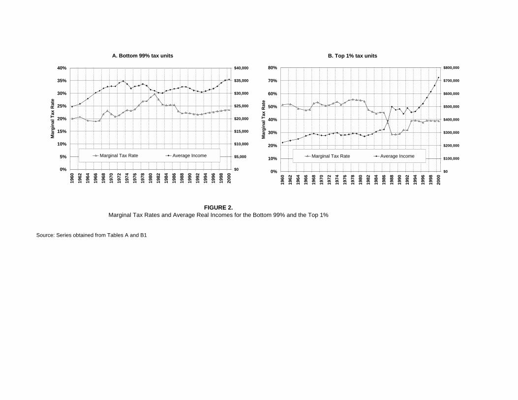
FIGURE 2.Marginal Tax Rates and Average Real Incomes for the Bottom 99% and the Top 1%

Source: Series obtained from Tables A and B1

A. Bottom 99% tax units

0%

5%

10%

15%

20%

25%

30%

35%

40%19

60

1962

1964

1966

1968

1970

1972

1974

1976

1978

1980

1982

1984

1986

1988

1990

1992

1994

1996

1998

2000

Mar

gin

al T

ax R

ate

$0

$5,000

$10,000

$15,000

$20,000

$25,000

$30,000

$35,000

$40,000

Marginal Tax Rate Average Income

B. Top 1% tax units

0%

10%

20%

30%

40%

50%

60%

70%

80%

1960

1962

1964

1966

1968

1970

1972

1974

1976

1978

1980

1982

1984

1986

1988

1990

1992

1994

1996

1998

2000

Mar

gin

al T

ax R

ate

$0

$100,000

$200,000

$300,000

$400,000

$500,000

$600,000

$700,000

$800,000

Marginal Tax Rate Average Income

FIGURE 3.Tax Rates and Income Shares for the Medium-High Income Groups

Source: Series obtained from Tables B1 and B2

A. Top 10-5% tax units

0%

5%

10%

15%

20%

25%

30%

35%

40%19

60

1962

1964

1966

1968

1970

1972

1974

1976

1978

1980

1982

1984

1986

1988

1990

1992

1994

1996

1998

2000

Mar

gin

al T

ax R

ate

0%

2%

4%

6%

8%

10%

12%

14%

16%

Inco

me

Sh

are

Marginal Tax Rate Income Share

B. Top 1-.5% tax units

0%

10%

20%

30%

40%

50%

60%

1960

1962

1964

1966

1968

1970

1972

1974

1976

1978

1980

1982

1984

1986

1988

1990

1992

1994

1996

1998

2000

Mar

gin

al T

ax R

ate

0%

1%

2%

3%

4%

5%

6%

Inco

me

Sh

are

Marginal Tax Rate Income Share

FIGURE 4.Tax Rates and Income Shares for the Very Top Groups

Source: Series obtained from Tables B1 and B2

A. Top 0.1-0.01% tax units

0%

10%

20%

30%

40%

50%

60%

70%19

60

1962

1964

1966

1968

1970

1972

1974

1976

1978

1980

1982

1984

1986

1988

1990

1992

1994

1996

1998

2000

Mar

gin

al T

ax R

ate

0.0%

0.5%

1.0%

1.5%

2.0%

2.5%

3.0%

3.5%

4.0%

4.5%

5.0%

Inco

me

Sh

are

Marginal Tax Rate Income Share

B. Top 0.01% tax units

0%

10%

20%

30%

40%

50%

60%

70%

80%

90%

1960

1962

1964

1966

1968

1970

1972

1974

1976

1978

1980

1982

1984

1986

1988

1990

1992

1994

1996

1998

2000

Mar

gin

al T

ax R

ate

0.0%

0.5%

1.0%

1.5%

2.0%

2.5%

3.0%

3.5%

Inco

me

Sh

are

Marginal Tax Rate Income Share

FIGURE 5.The Top 1% Income Share and fitted Values from Elasticity Regressions

Source: Series based on regression analysis presented in Table 3, columns (1) and (5).The diamond line is the top 1% income share. The dotted line is the fitted regression curveincluding only the net-of-tax rate. The solid line is the fitted regression curve including time controls.The dashed line is the same fitted regression curve but freezes the marginal tax rate at the 1960 value.

6%

8%

10%

12%

14%

16%

18%

19

60

19

62

19

64

19

66

19

68

19

70

19

72

19

74

19

76

19

78

19

80

19

82

19

84

19

86

19

88

19

90

19

92

19

94

19

96

19

98

20

00

Inc

om

e S

ha

re

Income Share(t)

A+1.58*log[1-MTR(t)]

A+0.62*log[1-MTR(t)]-.018*t+.00077*t^2

A+0.62*log[1-MTR(1960)]-.018*t+.00077*t^2

FIGURE 6.The Top 10% Income Share and Composition, 1960-2000

Source: Tables B1 and Table D1 in the working paper version Saez (2004).The figure displays the income share of the top 10% tax units, and how the top 10% incomes are divided into seven income components: wages and salaries (including exercised stock options), S-corporation profits, partnership profits, sole proprietorship profits, dividends, interest income, and other income.

0%

5%

10%

15%

20%

25%

30%

35%

40%

45%

50%19

60

1962

1964

1966

1968

1970

1972

1974

1976

1978

1980

1982

1984

1986

1988

1990

1992

1994

1996

1998

2000

Wages S-Corp. Partner. Sole P. Dividends Interest Other

FIGURE 7.The Top 1% Income Share and Composition, 1960-2000

Source: Tables B1 and Table D1 in the working paper version Saez (2004).The figure displays the income share of the top 1% tax units, and how the top 1% incomes are divided into seven income components: wages and salaries (including exercised stock options), S-corporation profits, partnership profits, sole proprietorship profits, dividends, interest income, and other income.

0%

2%

4%

6%

8%

10%

12%

14%

16%

18%19

60

1962

1964

1966

1968

1970

1972

1974

1976

1978

1980

1982

1984

1986

1988

1990

1992

1994

1996

1998

2000

Wages S-Corp. Partner. Sole P. Dividends Interest Other

FIGURE 8.The Top 0.01% Income Share and Composition, 1960-2000

Source: Tables B1 and Table D1 in the working paper version Saez (2004).The figure displays the income share of the top .01% tax units, and how the top .01% incomes are divided into seven income components: wages and salaries (including exercised stock options), S-corporation profits, partnership profits, sole proprietorship profits, dividends, interest income, and other income.

0.0%

0.5%

1.0%

1.5%

2.0%

2.5%

3.0%

3.5%19

60

1962

1964

1966

1968

1970

1972

1974

1976

1978

1980

1982

1984

1986

1988

1990

1992

1994

1996

1998

2000

Wages S-Corp. Partner. Sole P. Dividends Interest Other

FIGURE 9.Marginal Tax Rates and Average Real Wage Incomes for the Bottom 99% and the Top 1%

Source: Series obtained from Tables A, C1, and C2.

A. Bottom 99% tax units with wage income

0%

5%

10%

15%

20%

25%

30%

35%

40%

45%19

60

1962

1964

1966

1968

1970

1972

1974

1976

1978

1980

1982

1984

1986

1988

1990

1992

1994

1996

1998

2000

Mar

gin

al T

ax R

ate

$0

$5,000

$10,000

$15,000

$20,000

$25,000

$30,000

$35,000

$40,000

$45,000

Marginal Tax Rate Average Income

B. Top 1% tax units with wage income

0%

10%

20%

30%

40%

50%

60%

1960

1962

1964

1966

1968

1970

1972

1974

1976

1978

1980

1982

1984

1986

1988

1990

1992

1994

1996

1998

2000

Mar

gin

al T

ax R

ate

$0

$100,000

$200,000

$300,000

$400,000

$500,000

$600,000

Marginal Tax Rate Average Income

TABLE 1.

Percentile threshold

Income threshold Income Groups

Number of tax units

Average income in each

group

(1) (2) (3) (4) (5)

Full Population 133,589,000 $42,709

Median $25,076 Bottom 90% 120,230,100 $26,616

Top 10% $87,334 Top 10-5% 6,679,450 $100,480

Top 5% $120,212 Top 5-1% 5,343,560 $162,366

Top 1% $277,983 Top 1-0.5% 667,945 $327,970

Top .5% $397,949 Top 0.5-0.1% 534,356 $611,848

Top .1% $1,134,849 Top 0.1-0.01% 120,230 $2,047,801

Top .01% $5,349,795 Top 0.01% 13,359 $13,055,242

Notes: Computations based on income tax return statistics.

Income defined as annual gross income reported on tax returns excluding capital gains and all government transfers

(such as Social Security, Unemployment Benefits, Welfare Payments, etc.) and before individual income taxes and

employees' payroll taxes. Amounts are expressed in current 2000 dollars.

Column (2) reports the income thresholds corresponding to each of the percentiles in column (1). For example,

an annual income of at least $87,334 is required to belong to the top 10% tax units, etc.

Thresholds and Average Incomes in Top Income Groups in 2000

TABLE 2.Elasticities of income wrt net-of-tax rates in the Aggregate, Bottom 99%, and Top 1%

Regression Regression Regressionin Levels in Levels + in Levels +

Time ControlTime Controls(1) (2) (3)

PANEL A. All tax unitsElasticity -0.44 -0.02 0.20

(0.84) (0.38) (0.55)Time Trend YES YESTime Trend Square YES

PANEL B. Bottom 99% tax unitsElasticity -0.66 -0.41 -0.04

(0.70) (0.37) (0.38)Time Trend YES YESTime Trend Square YES

PANEL C. Top 1% tax units Elasticity 1.83 0.71 0.50

(0.37) (0.22) (0.18)Time Trend YES YESTime Trend Square YES

Notes: Estimates obtained by time-series regression of log(average real income) (using CPI-U deflator)

on a constant, log (1 - average marginal tax rate) from 1960 to 2000 (38 observations).

In column 1, simple OLS regression is run, Standard Errors from Newey-West with 8 lags.

In column 2, a time trend is added. In column 3, time^2 trend is added.

TABLE 3.Elasticities of the top 1% income share with respect to net-of-tax rates

OLS 2SLS OLS 2SLS OLS 2SLS OLS 2SLS(Newey-West (Top Rate (Newey-West (Top Rate (Newey-West (Top Rate (Newey-West (Top Rate

s.e.) Instrument) s.e.) Instrument) s.e.) Instrument) s.e.) Instrument)(1) (2) (3) (4) (5) (6) (7) (8)

Elasticity 1.58 1.70 0.85 -0.02 0.62 0.59 0.68 0.61(0.28) (0.19) (0.21) (0.34) (0.12) (0.08) (0.15) (0.09)

Time Trend YES YES YES YES YES YES

Time Trend Square YES YES YES YES

Time Trend Cube YES YES

Adjusted R-Square 0.72 0.71 0.86 0.74 0.98 0.98 0.98 0.98

First Stage t-statistics 10.10 5.37 10.1 11.7

Notes: Estimates obtained by time-series regression of log(top 1% income share)

on a constant, log (1 - average marginal tax rate), and polynomials time controls from 1960 to 2000 (38 observations).

In columns 1, 3, 5, and 7, simple OLS regression is run, Standard Errors from Newey-West with 8 lags.

In columns 2, 4, 6, and 8, 2SLS regression is run using log(1- top marginal tax rate) as an instrument.

TABLE 4.Elasticities of income shares wrt net-of-tax rates for various upper income groups

Newey-West Newey-West 2SLS Newey-West Newey-West 2SLSOLS Regression OLS Regression Regression OLS Regression OLS Regression Regressionno time controls with time controlswith time controls no time controls with time controlswith time controls

(1) (2) (3) (4) (5) (6)

A. Top Income Groups B. Intermediate Income Groups

Top 10% Top 10-5%Elasticity 0.77 0.33 0.32 -0.44 -0.11 -0.04

(0.36) (0.08) (0.05) (0.17) (0.09) (0.10)First-Stage t-stat. of instrument 9.94 6.5

Top 5% Top 5-1%Elasticity 1.25 0.43 0.39 0.14 0.12 0.09

(0.30) (0.09) (0.05) (0.28) (0.04) (0.04)First-Stage t-stat. of instrument 10.5 8.16

Top 1% Top 1-.5%Elasticity 1.58 0.62 0.59 0.92 0.30 0.29

(0.28) (0.12) (0.08) (0.21) (0.08) (0.07)First-Stage t-stat. of instrument 10.11 10.65

Top 0.5% Top 0.5-0.1%Elasticity 1.55 0.72 0.69 1.21 0.52 0.49

(0.25) (0.13) (0.09) (0.22) (0.09) (0.08)First-Stage t-stat. of instrument 9.9 9.21

Top 0.1% Top 0.1-0.01%Elasticity 1.54 0.94 0.89 1.44 0.78 0.76

(0.27) (0.19) (0.11) (0.23) (0.16) (0.11)First-Stage t-stat. of instrument 11.37 9.69

Top 0.01% Top 0.01%Elasticity 1.45 1.08 1.09 1.45 1.08 1.09

(0.36) (0.32) (0.16) (0.36) (0.32) (0.16)First-Stage t-stat. of instrument 18.01 18.01

Notes: Estimates obtained by time-series regression of log(top income share)

on a constant, log (1 - average marginal tax rate), time trend, and square of time trend from 1960 to 2000 (38 observations).

In columns 1 and 4, OLS regression is run, no time trend included. Newey-West standard errors with 8 lags reported.

In columns 2 and 5, OLS regression is run with time and time^2 trend included. Newey-West standard errors with 8 lags reported.

In columns 3 and 6, 2SLS regression is run with time and time^2 trend included and instrumented with log (1- top marginal tax rate).

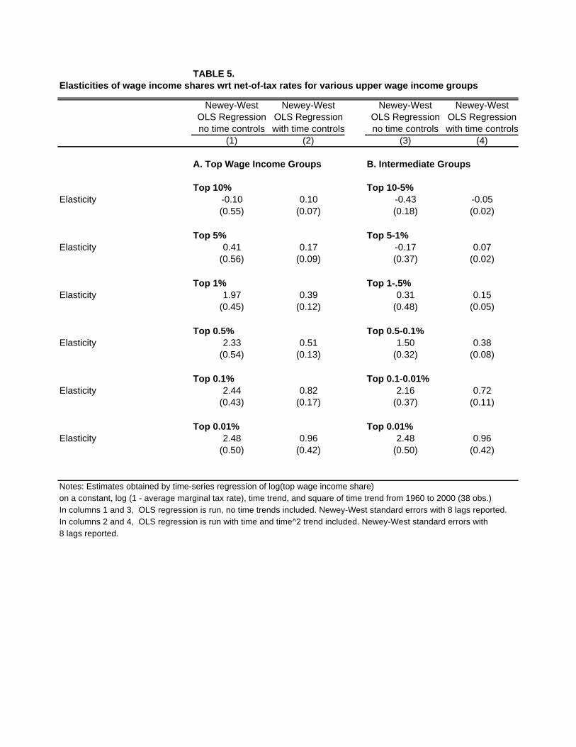
TABLE 5.Elasticities of wage income shares wrt net-of-tax rates for various upper wage income groups

Newey-West Newey-West Newey-West Newey-WestOLS Regression OLS Regression OLS Regression OLS Regressionno time controls with time controls no time controls with time controls

(1) (2) (3) (4)

A. Top Wage Income Groups B. Intermediate Groups

Top 10% Top 10-5%Elasticity -0.10 0.10 -0.43 -0.05

(0.55) (0.07) (0.18) (0.02)

Top 5% Top 5-1%Elasticity 0.41 0.17 -0.17 0.07

(0.56) (0.09) (0.37) (0.02)

Top 1% Top 1-.5%Elasticity 1.97 0.39 0.31 0.15

(0.45) (0.12) (0.48) (0.05)

Top 0.5% Top 0.5-0.1%Elasticity 2.33 0.51 1.50 0.38

(0.54) (0.13) (0.32) (0.08)

Top 0.1% Top 0.1-0.01%Elasticity 2.44 0.82 2.16 0.72

(0.43) (0.17) (0.37) (0.11)

Top 0.01% Top 0.01%Elasticity 2.48 0.96 2.48 0.96

(0.50) (0.42) (0.50) (0.42)

Notes: Estimates obtained by time-series regression of log(top wage income share)

on a constant, log (1 - average marginal tax rate), time trend, and square of time trend from 1960 to 2000 (38 obs.)

In columns 1 and 3, OLS regression is run, no time trends included. Newey-West standard errors with 8 lags reported.

In columns 2 and 4, OLS regression is run with time and time^2 trend included. Newey-West standard errors with

8 lags reported.

(1) (2) (3) (4) (5) (8) (9) (10) (11) (12) (13) (14) (15) (16)Tax Units Number of (2)/(1) Population (4)/(1) Total income Average incomeAverage Marginal Tax Units with Total Wages Average WagesAverage Marginal CPI-U CPI-U-RS

tax returns (%) (millions 2000 $(2000 $, CPI-U) Tax Rate (%) Wages (millions 2000 $,(2000 $, CPI-U) Tax Rate (%) (2000 base) (2000 base)('000s) ('000s) ('000s) CPI-U) CPI-U)

1960 68,681 61,028 88.9 180,671 2.63 1,850,218 26,939 22.55 52,554 1,587,214 30,201 22.68 17.189 20.1831961 69,997 61,499 87.9 183,691 2.62 1,907,985 27,258 51,946 1,615,622 31,102 17.361 20.3851962 71,254 62,712 88.0 186,538 2.62 2,011,233 28,226 23.32 53,338 1,705,361 31,972 23.35 17.552 20.6091963 72,464 63,943 88.2 189,242 2.61 2,099,285 28,970 53,893 1,772,347 32,886 17.762 20.8561964 73,660 65,376 88.8 191,889 2.61 2,236,911 30,368 21.64 55,216 1,877,056 33,995 21.66 17.993 21.1271965 74,772 67,596 90.4 194,303 2.60 2,361,753 31,586 57,239 1,987,572 34,724 18.299 21.4861966 75,831 70,160 92.5 196,560 2.59 2,500,162 32,970 21.30 60,358 2,125,707 35,219 21.19 18.830 22.1101967 76,856 71,652 93.2 198,712 2.59 2,600,178 33,832 21.62 61,571 2,213,824 35,955 21.59 19.376 22.7511968 77,826 73,729 94.7 200,706 2.58 2,719,064 34,938 24.33 62,836 2,337,364 37,198 24.10 20.190 23.6621969 78,793 75,834 96.2 202,677 2.57 2,794,675 35,469 25.53 64,371 2,435,448 37,834 25.15 21.280 24.6931970 79,924 74,280 92.9 205,052 2.57 2,845,542 35,603 24.11 63,778 2,447,144 38,370 24.20 22.535 25.8821971 81,849 74,576 91.1 207,661 2.54 2,905,636 35,500 23.06 63,194 2,484,179 39,311 23.29 23.527 27.0311972 83,670 77,573 92.7 209,896 2.51 3,093,721 36,975 23.62 64,750 2,630,468 40,625 23.73 24.280 27.8641973 85,442 80,693 94.4 211,909 2.48 3,225,502 37,751 24.77 67,614 2,748,251 40,646 24.68 25.785 29.6081974 87,228 83,340 95.5 213,854 2.45 3,195,330 36,632 25.82 68,518 2,697,802 39,373 25.61 28.621 32.5411975 89,127 82,229 92.3 215,973 2.42 3,093,548 34,709 25.40 66,671 2,609,012 39,132 25.91 31.226 35.2361976 91,048 84,670 93.0 218,035 2.39 3,235,043 35,531 26.04 68,459 2,722,938 39,775 26.53 33.037 37.2571977 93,076 86,635 93.1 220,239 2.37 3,339,935 35,884 27.71 70,898 2,825,066 39,847 28.33 35.185 39.6351978 95,213 89,771 94.3 222,585 2.34 3,480,248 36,552 29.16 74,503 2,961,075 39,745 29.87 37.859 41.3401979 97,457 92,694 95.1 225,055 2.31 3,503,689 35,951 29.19 77,038 2,979,812 38,680 30.04 42.137 45.2241980 99,625 93,902 94.3 227,726 2.29 3,412,006 34,248 30.66 76,913 2,880,118 37,446 31.77 47.825 50.2581981 101,432 95,396 94.0 229,966 2.27 3,419,549 33,713 31.68 77,439 2,876,292 37,143 32.95 52.751 54.9741982 103,250 95,337 92.3 232,188 2.25 3,405,788 32,986 29.22 75,771 2,844,255 37,537 30.71 56.022 58.1851983 105,067 96,321 91.7 234,307 2.23 3,466,971 32,998 27.36 76,260 2,913,254 38,202 28.90 57.814 60.6021984 106,871 99,439 93.0 236,348 2.21 3,637,968 34,041 26.99 80,008 3,075,930 38,445 28.36 60.300 63.0201985 108,736 101,660 93.5 238,466 2.19 3,760,935 34,588 27.27 81,936 3,193,778 38,979 28.59 62.471 65.1611986 110,684 103,045 93.1 240,651 2.17 3,876,141 35,020 27.26 83,340 3,321,487 39,855 28.77 63.658 66.3101987 112,640 106,996 95.0 242,804 2.16 4,046,941 35,928 24.47 85,618 3,442,337 40,206 25.98 65.950 68.5691988 114,656 109,708 95.7 245,021 2.14 4,305,720 37,553 22.92 88,121 3,572,571 40,542 24.75 68.654 71.0661989 116,759 112,136 96.0 247,342 2.12 4,350,842 37,263 23.06 90,145 3,609,277 40,039 24.65 71.949 74.1581990 119,055 113,717 95.5 250,132 2.10 4,377,181 36,766 23.05 91,348 3,632,403 39,764 24.77 75.834 77.8831991 120,453 114,730 95.2 253,493 2.10 4,286,889 35,590 23.11 89,813 3,574,052 39,794 24.61 79.019 80.7371992 121,944 113,605 93.2 256,894 2.11 4,356,547 35,726 22.99 89,883 3,645,188 40,555 24.91 81.390 82.8781993 123,378 114,602 92.9 260,255 2.11 4,320,595 35,019 23.94 91,279 3,687,902 40,402 25.60 83.832 85.0181994 124,716 115,943 93.0 263,436 2.11 4,424,217 35,474 24.29 93,270 3,783,593 40,566 25.82 86.011 86.8811995 126,023 118,218 93.8 266,557 2.12 4,581,375 36,353 24.58 95,388 3,891,745 40,799 26.29 88.419 89.0611996 127,625 120,351 94.3 269,667 2.11 4,730,336 37,064 24.75 97,338 3,986,011 40,950 26.65 91.072 91.4781997 129,301 122,422 94.7 272,912 2.11 4,974,958 38,476 25.33 100,161 4,170,993 41,643 27.32 93.167 93.4601998 130,945 124,771 95.3 276,115 2.11 5,268,063 40,231 25.56 103,069 4,429,422 42,975 27.79 94.657 94.7681999 132,267 127,075 96.1 279,295 2.11 5,522,779 41,755 25.84 105,233 4,626,416 43,963 28.39 96.740 96.7502000 133,589 129,272 96.8 282,339 2.11 5,705,414 42,709 26.13 107,693 4,836,329 44,909 28.99 100.000 100.000

Notes: Population and tax units estimates based on census and current population surveys (Historical Statistics of the United States, and Statistical Abstract of the United States)Tax units estimated as sum of married men, divorced and widowed men and women, and singles men and women aged 20 and over.Income defined as Adjusted Gross Income less realized capital gains, taxable SS and UI benefits and adding back all adjustments to gross income. Income of non-filers is imputed as 20% of average income.Marginal tax rates are weighted by income and estimated using TAXSIM calculator and the tax return micro-files and ignoring interactions with state income taxes.Marginal income tax rate in column (10) is a weighted average of marginal tax rate on earned income and other income.Tax units with wages defined as total number of employees (from National Income and Product Accounts) less number of married women employed (from Statistical Abstract of the United States).Total wages from total compensation of employees from National Income and Product Accounts.Marginal income tax rate in column (14) is the average (wage income weighted) marginal tax rate on wages and salaries.Consumer Price Index (CPI-U) is the official CPI index from Economic Report of the President. CPI-U-RS includes retrospectively improvements on CPI estimation method for 1967-1998 period.

TABLE A. Reference Totals for Population, Income, and Inflation, 1960-2000Tax Units and Population Inflation IndexesTotal Income Wage earners and wage income

Top 10% Top 5% Top 1% Top .5% Top .1% Top .01% Top 10-5% Top 5-1% Top 1-.5% Top .5-.1% Top .1-.01% Top .01%

(1) (2) (3) (4) (5) (6) (7) (8) (9) (10) (11) (12)

1960 31.70 20.81 8.28 5.53 2.13 0.59 10.89 12.53 2.75 3.40 1.54 0.591962 32.37 21.23 8.42 5.59 2.10 0.57 11.14 12.81 2.83 3.49 1.53 0.571964 32.18 21.04 8.25 5.46 2.05 0.56 11.14 12.78 2.80 3.41 1.49 0.561966 32.01 21.01 8.35 5.56 2.14 0.60 11.00 12.66 2.79 3.42 1.54 0.601967 32.12 21.12 8.42 5.61 2.15 0.59 11.00 12.70 2.80 3.47 1.56 0.591968 32.06 21.03 8.36 5.58 2.13 0.58 11.02 12.67 2.78 3.44 1.56 0.581969 31.86 20.72 8.03 5.30 1.99 0.54 11.14 12.70 2.73 3.31 1.45 0.541970 31.59 20.45 7.81 5.15 1.92 0.52 11.14 12.64 2.66 3.22 1.40 0.521971 31.82 20.54 7.79 5.11 1.90 0.51 11.28 12.76 2.68 3.21 1.39 0.511972 31.70 20.43 7.76 5.09 1.90 0.52 11.27 12.67 2.67 3.19 1.39 0.521973 31.93 20.64 7.75 5.06 1.87 0.49 11.29 12.89 2.69 3.19 1.38 0.491974 32.47 21.12 8.15 5.41 2.09 0.56 11.35 12.98 2.74 3.32 1.53 0.561975 32.74 21.14 8.04 5.32 2.02 0.55 11.61 13.09 2.73 3.29 1.47 0.551976 32.56 20.97 7.92 5.23 2.00 0.56 11.59 13.04 2.69 3.23 1.45 0.561977 32.60 20.99 7.96 5.27 2.03 0.56 11.60 13.04 2.69 3.24 1.47 0.561978 32.63 21.05 8.01 5.32 2.07 0.57 11.59 13.03 2.69 3.25 1.49 0.571979 32.53 21.01 8.09 5.40 2.15 0.61 11.52 12.91 2.69 3.26 1.54 0.611980 33.05 21.36 8.24 5.53 2.22 0.65 11.69 13.11 2.71 3.31 1.57 0.651981 32.96 21.16 8.03 5.38 2.17 0.64 11.80 13.13 2.65 3.21 1.54 0.641982 33.81 21.83 8.50 5.79 2.45 0.77 11.99 13.32 2.72 3.34 1.68 0.771983 34.37 22.25 8.71 5.99 2.60 0.86 12.12 13.55 2.72 3.39 1.74 0.861984 34.54 22.50 8.98 6.26 2.82 0.97 12.03 13.52 2.72 3.44 1.84 0.971985 34.86 22.81 9.20 6.44 2.94 0.96 12.05 13.61 2.76 3.50 1.98 0.961986 35.20 23.02 9.22 6.41 2.86 0.99 12.18 13.80 2.81 3.55 1.87 0.991987 36.68 24.70 10.87 7.83 3.74 1.30 11.98 13.83 3.04 4.09 2.44 1.301988 38.85 27.17 13.28 10.02 5.22 1.99 11.68 13.89 3.26 4.80 3.23 1.991989 38.70 26.89 12.74 9.45 4.76 1.75 11.82 14.15 3.29 4.69 3.02 1.751990 39.12 27.32 13.12 9.79 4.92 1.83 11.81 14.20 3.32 4.88 3.09 1.831991 39.00 26.98 12.48 9.12 4.44 1.61 12.02 14.50 3.36 4.68 2.83 1.611992 40.36 28.35 13.71 10.25 5.26 2.03 12.01 14.65 3.46 4.99 3.23 2.031993 39.99 27.85 13.03 9.58 4.75 1.75 12.14 14.82 3.45 4.83 3.01 1.751994 39.93 27.85 13.04 9.57 4.74 1.74 12.08 14.81 3.47 4.82 3.00 1.741995 40.54 28.46 13.53 9.99 4.98 1.82 12.08 14.93 3.54 5.00 3.17 1.821996 41.14 29.15 14.10 10.48 5.32 1.97 11.99 15.05 3.62 5.16 3.35 1.971997 41.70 29.83 14.77 11.12 5.80 2.19 11.87 15.07 3.65 5.31 3.61 2.191998 42.06 30.31 15.28 11.60 6.19 2.40 11.74 15.04 3.68 5.41 3.79 2.401999 42.59 30.91 15.85 12.14 6.63 2.63 11.68 15.06 3.71 5.51 4.00 2.632000 43.91 32.15 16.94 13.10 7.37 3.06 11.76 15.21 3.84 5.73 4.32 3.06

Notes: Computations by authors on tax return statistics. Taxpayers are ranked by gross income (excluding capital gains and government transfers).

Income of non-filers is imputed as 20% of average income. Groups defined relative to all tax units (filers and non-filers).The Table reports the percentage of total income accruing to each of the top groups. Top 10% denotes to top decile,

top 10-5% denotes the bottom half of the top decile, etc.

Table B1. Top Income Shares in the United States, 1960-2000

Top 10% Top 5% Top 1% Top .5% Top .1% Top .01% Top 10-5% Top 5-1% Top 1-.5% Top .5-.1% Top .1-.01% Top MTR

(1) (2) (3) (4) (5) (6) (7) (8) (9) (10) (11) (12)

1960 32.32 37.33 51.47 57.92 69.89 81.30 22.74 27.98 38.50 50.42 65.55 871962 33.17 38.02 51.89 58.05 69.07 79.31 23.92 28.91 39.73 51.41 65.27 871964 31.19 35.72 48.43 54.00 62.78 70.43 22.65 27.51 37.54 48.71 59.89 771966 30.58 34.91 47.13 52.00 59.90 65.22 22.32 26.85 37.42 47.06 57.84 701967 31.05 35.49 47.61 52.29 59.67 64.74 22.53 27.46 38.25 47.72 57.74 701968 34.55 39.38 52.37 57.03 64.31 67.44 25.32 30.82 43.03 52.51 63.15 75.251969 35.56 40.40 53.37 58.04 65.22 68.62 26.54 32.21 44.30 53.72 63.95 771970 34.29 39.05 51.53 55.76 61.87 64.28 25.57 31.34 43.33 52.12 60.98 71.751971 33.48 38.30 50.73 54.89 61.06 63.50 24.71 30.72 42.78 51.24 60.16 701972 34.55 39.42 51.19 54.48 59.36 61.40 25.72 32.22 44.94 51.57 58.60 701973 36.19 41.26 52.37 55.36 60.14 63.22 26.91 34.58 46.74 52.55 59.04 701974 37.56 42.73 53.79 56.56 61.20 63.68 27.95 35.78 48.32 53.64 60.30 701975 36.53 41.12 51.38 54.52 59.34 61.87 28.18 34.82 45.28 51.55 58.38 701976 38.32 43.02 53.10 56.04 60.77 64.36 29.82 36.89 47.39 53.10 59.40 701977 40.88 45.90 54.93 56.89 60.12 61.74 31.81 40.39 51.09 54.87 59.50 701978 42.65 47.43 55.45 57.37 60.62 62.75 33.96 42.50 51.67 55.30 59.80 701979 42.57 47.44 54.99 56.53 58.61 59.90 33.70 42.70 51.91 55.15 58.10 701980 44.14 48.46 54.84 56.18 57.79 58.79 36.25 44.46 52.10 55.11 57.37 701981 45.01 48.72 54.12 55.20 56.11 56.30 38.36 45.41 51.92 54.59 56.03 701982 40.60 43.72 47.44 47.45 46.49 44.90 34.92 41.34 47.44 48.15 47.22 501983 38.24 41.27 46.07 47.17 47.48 47.15 32.68 38.18 43.66 46.92 47.65 501984 37.33 40.22 44.65 45.72 45.88 46.56 31.92 37.28 42.18 45.59 45.53 501985 37.74 40.73 45.53 46.81 47.14 47.16 32.09 37.49 42.54 46.53 47.13 501986 37.58 40.52 45.34 46.51 47.31 46.72 32.03 37.30 42.66 45.87 47.62 501987 33.88 35.85 37.31 37.07 36.93 36.53 29.82 34.69 37.92 37.21 37.14 38.51988 29.03 29.46 28.59 27.53 27.33 27.07 28.05 30.29 31.83 27.76 27.49 281989 29.10 29.56 28.50 27.42 27.09 26.99 28.05 30.51 31.60 27.75 27.15 281990 29.20 29.74 28.91 27.90 27.65 27.57 27.96 30.50 31.90 28.15 27.70 281991 29.93 30.99 32.01 31.50 31.29 31.21 27.57 30.11 33.39 31.70 31.35 311992 29.87 30.88 31.83 31.34 31.25 31.15 27.47 30.00 33.29 31.42 31.32 311993 32.34 34.38 39.01 39.55 39.99 39.83 27.66 30.31 37.50 39.12 40.08 39.61994 32.57 34.61 39.27 39.68 39.95 39.80 27.86 30.51 38.14 39.41 40.04 39.61995 32.62 34.60 38.74 38.98 39.51 39.46 27.94 30.86 38.04 38.47 39.53 39.61996 32.39 34.17 37.74 37.90 38.42 38.38 28.05 30.83 37.26 37.37 38.44 39.61997 33.21 35.21 39.15 39.47 39.48 39.35 28.18 31.35 38.16 39.47 39.55 39.61998 33.63 35.54 39.05 39.36 39.43 39.37 28.69 31.98 38.07 39.29 39.47 39.61999 33.79 35.78 38.94 39.32 39.32 39.19 28.53 32.45 37.67 39.32 39.41 39.62000 33.95 36.02 38.83 39.28 39.21 39.01 28.37 32.93 37.27 39.35 39.35 39.6

Notes: Marginal Tax Rates computed using micro-files of tax returns and the TAXSIM calculator. Marginal tax rates include only federal income taxes and ignore state

income taxes. Marginal tax rates are weighted by income, and are a weighted average of marginal tax rates on earnings and other income (excluding capital gains).

Column (12) reports the top marginal tax rate. In 1960-1963, the top bracket rate is 91% but there is maximum average tax rate of 87%.

In 1971-1981, the top marginal tax rate for labor income is lower (see Table D2).

Table B2. Marginal Tax Rates for Top Income Groups in the United States, 1960-2000

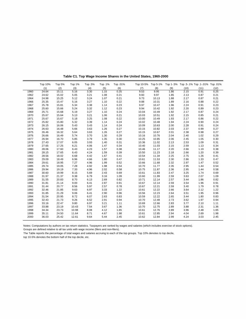
Top 10% Top 5% Top 1% Top .5% Top .1% Top .01% Top 10-5% Top 5-1% Top 1-.5% Top .5-.1% Top .1-.01% Top .01%

(1) (2) (3) (4) (5) (6) (7) (8) (9) (10) (11) (12)1960 24.64 15.11 5.16 3.30 1.15 0.25 9.53 9.95 1.86 2.15 0.91 0.251962 24.62 15.02 5.05 3.21 1.08 0.21 9.60 9.97 1.85 2.13 0.87 0.211964 24.98 15.25 5.12 3.24 1.07 0.21 9.73 10.13 1.88 2.17 0.87 0.211966 25.35 15.47 5.16 3.27 1.10 0.22 9.88 10.31 1.89 2.16 0.88 0.221967 25.78 15.81 5.34 3.38 1.14 0.23 9.97 10.47 1.96 2.24 0.91 0.231968 25.60 15.66 5.24 3.32 1.12 0.23 9.94 10.42 1.92 2.20 0.89 0.231969 25.71 15.68 5.19 3.27 1.10 0.24 10.04 10.49 1.92 2.17 0.87 0.241970 25.67 15.64 5.13 3.21 1.06 0.21 10.03 10.51 1.92 2.15 0.85 0.211971 25.67 15.67 5.18 3.25 1.08 0.22 10.00 10.49 1.93 2.17 0.86 0.221972 25.82 15.80 5.32 3.39 1.14 0.24 10.02 10.48 1.94 2.24 0.90 0.241973 26.15 16.06 5.43 3.43 1.14 0.24 10.09 10.63 2.00 2.28 0.91 0.241974 26.63 16.48 5.66 3.63 1.26 0.27 10.15 10.82 2.03 2.37 0.99 0.271975 26.46 16.32 5.64 3.63 1.26 0.27 10.15 10.67 2.01 2.38 0.98 0.271976 26.66 16.49 5.74 3.70 1.30 0.29 10.16 10.76 2.04 2.40 1.02 0.291977 26.94 16.70 5.85 3.79 1.35 0.30 10.25 10.85 2.06 2.45 1.05 0.301978 27.43 17.07 6.05 3.93 1.40 0.31 10.36 11.02 2.13 2.53 1.09 0.311979 27.65 17.25 6.21 4.06 1.47 0.34 10.40 11.03 2.15 2.59 1.13 0.341980 28.06 17.60 6.43 4.23 1.57 0.38 10.46 11.17 2.20 2.66 1.19 0.381981 28.15 17.65 6.43 4.24 1.59 0.39 10.50 11.23 2.18 2.66 1.20 0.391982 28.56 18.02 6.68 4.42 1.67 0.41 10.54 11.34 2.25 2.75 1.26 0.411983 29.09 18.49 6.96 4.66 1.80 0.47 10.61 11.53 2.30 2.86 1.33 0.471984 29.61 18.95 7.27 4.96 1.99 0.52 10.66 11.68 2.32 2.97 1.47 0.521985 29.74 19.05 7.28 4.92 1.98 0.54 10.70 11.77 2.35 2.95 1.44 0.541986 29.94 19.19 7.33 4.96 2.02 0.58 10.75 11.87 2.36 2.95 1.44 0.581987 30.60 19.99 8.15 5.69 2.43 0.69 10.61 11.83 2.47 3.25 1.74 0.691988 31.97 21.37 9.38 6.79 3.16 1.09 10.60 11.99 2.59 3.63 2.07 1.091989 31.55 20.83 8.70 6.13 2.69 0.82 10.71 12.14 2.57 3.44 1.86 0.821990 31.81 21.14 9.00 6.41 2.87 0.91 10.67 12.14 2.59 3.54 1.96 0.911991 31.44 20.77 8.56 5.97 2.57 0.78 10.67 12.21 2.59 3.40 1.79 0.781992 32.46 21.85 9.63 6.97 3.33 1.22 10.61 12.22 2.66 3.64 2.12 1.221993 31.85 21.29 9.06 6.41 2.90 0.96 10.56 12.23 2.64 3.51 1.95 0.961994 31.54 20.95 8.72 6.07 2.63 0.83 10.59 12.22 2.65 3.44 1.80 0.831995 32.43 21.73 9.26 6.52 2.91 0.94 10.70 12.48 2.73 3.62 1.97 0.941996 33.16 22.47 9.80 6.97 3.21 1.11 10.69 12.66 2.83 3.77 2.10 1.111997 33.88 23.19 10.43 7.54 3.67 1.36 10.70 12.75 2.89 3.88 2.31 1.361998 34.34 23.73 10.98 8.08 4.12 1.65 10.61 12.76 2.89 3.96 2.48 1.651999 35.11 24.50 11.64 8.71 4.67 1.98 10.61 12.85 2.94 4.04 2.69 1.982000 36.03 25.42 12.61 9.64 5.44 2.45 10.62 12.84 2.99 4.24 3.03 2.45

Notes: Computations by authors on tax return statistics. Taxpayers are ranked by wages and salaries (which includes exercise of stock options).Groups are defined relative to all tax units with wage income (filers and non-filers).

The Table reports the percentage of total wages and salaries accruing to each of the top groups. Top 10% denotes to top decile,

top 10-5% denotes the bottom half of the top decile, etc.

Table C1. Top Wage Income Shares in the United States, 1960-2000

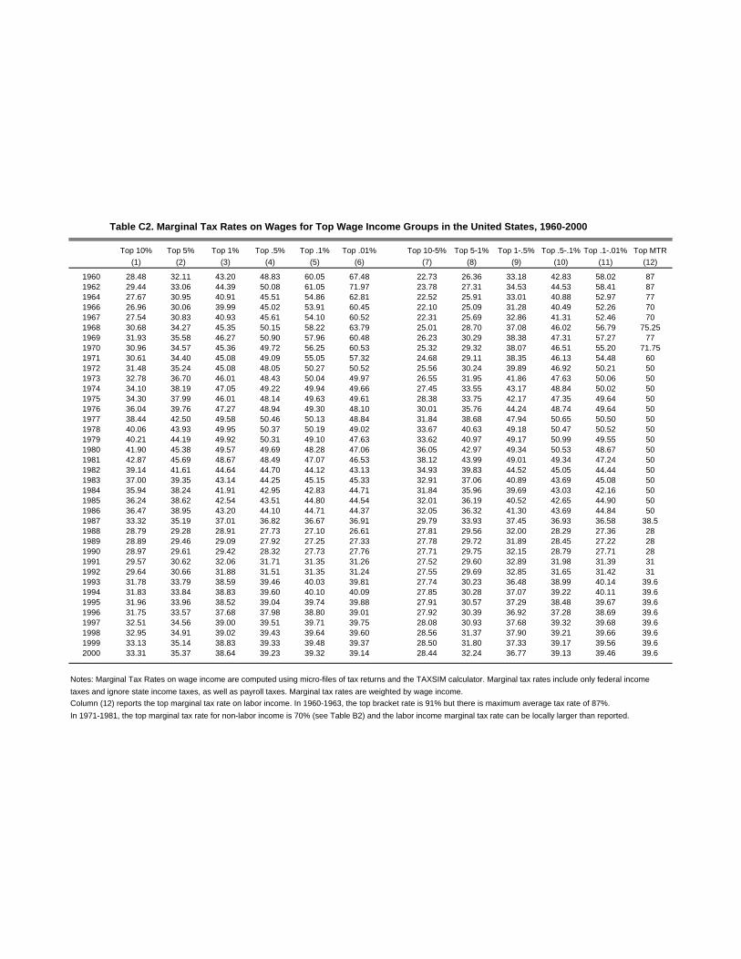
Top 10% Top 5% Top 1% Top .5% Top .1% Top .01% Top 10-5% Top 5-1% Top 1-.5% Top .5-.1% Top .1-.01% Top MTR

(1) (2) (3) (4) (5) (6) (7) (8) (9) (10) (11) (12)

1960 28.48 32.11 43.20 48.83 60.05 67.48 22.73 26.36 33.18 42.83 58.02 871962 29.44 33.06 44.39 50.08 61.05 71.97 23.78 27.31 34.53 44.53 58.41 871964 27.67 30.95 40.91 45.51 54.86 62.81 22.52 25.91 33.01 40.88 52.97 771966 26.96 30.06 39.99 45.02 53.91 60.45 22.10 25.09 31.28 40.49 52.26 701967 27.54 30.83 40.93 45.61 54.10 60.52 22.31 25.69 32.86 41.31 52.46 701968 30.68 34.27 45.35 50.15 58.22 63.79 25.01 28.70 37.08 46.02 56.79 75.251969 31.93 35.58 46.27 50.90 57.96 60.48 26.23 30.29 38.38 47.31 57.27 771970 30.96 34.57 45.36 49.72 56.25 60.53 25.32 29.32 38.07 46.51 55.20 71.751971 30.61 34.40 45.08 49.09 55.05 57.32 24.68 29.11 38.35 46.13 54.48 601972 31.48 35.24 45.08 48.05 50.27 50.52 25.56 30.24 39.89 46.92 50.21 501973 32.78 36.70 46.01 48.43 50.04 49.97 26.55 31.95 41.86 47.63 50.06 501974 34.10 38.19 47.05 49.22 49.94 49.66 27.45 33.55 43.17 48.84 50.02 501975 34.30 37.99 46.01 48.14 49.63 49.61 28.38 33.75 42.17 47.35 49.64 501976 36.04 39.76 47.27 48.94 49.30 48.10 30.01 35.76 44.24 48.74 49.64 501977 38.44 42.50 49.58 50.46 50.13 48.84 31.84 38.68 47.94 50.65 50.50 501978 40.06 43.93 49.95 50.37 50.19 49.02 33.67 40.63 49.18 50.47 50.52 501979 40.21 44.19 49.92 50.31 49.10 47.63 33.62 40.97 49.17 50.99 49.55 501980 41.90 45.38 49.57 49.69 48.28 47.06 36.05 42.97 49.34 50.53 48.67 501981 42.87 45.69 48.67 48.49 47.07 46.53 38.12 43.99 49.01 49.34 47.24 501982 39.14 41.61 44.64 44.70 44.12 43.13 34.93 39.83 44.52 45.05 44.44 501983 37.00 39.35 43.14 44.25 45.15 45.33 32.91 37.06 40.89 43.69 45.08 501984 35.94 38.24 41.91 42.95 42.83 44.71 31.84 35.96 39.69 43.03 42.16 501985 36.24 38.62 42.54 43.51 44.80 44.54 32.01 36.19 40.52 42.65 44.90 501986 36.47 38.95 43.20 44.10 44.71 44.37 32.05 36.32 41.30 43.69 44.84 501987 33.32 35.19 37.01 36.82 36.67 36.91 29.79 33.93 37.45 36.93 36.58 38.51988 28.79 29.28 28.91 27.73 27.10 26.61 27.81 29.56 32.00 28.29 27.36 281989 28.89 29.46 29.09 27.92 27.25 27.33 27.78 29.72 31.89 28.45 27.22 281990 28.97 29.61 29.42 28.32 27.73 27.76 27.71 29.75 32.15 28.79 27.71 281991 29.57 30.62 32.06 31.71 31.35 31.26 27.52 29.60 32.89 31.98 31.39 311992 29.64 30.66 31.88 31.51 31.35 31.24 27.55 29.69 32.85 31.65 31.42 311993 31.78 33.79 38.59 39.46 40.03 39.81 27.74 30.23 36.48 38.99 40.14 39.61994 31.83 33.84 38.83 39.60 40.10 40.09 27.85 30.28 37.07 39.22 40.11 39.61995 31.96 33.96 38.52 39.04 39.74 39.88 27.91 30.57 37.29 38.48 39.67 39.61996 31.75 33.57 37.68 37.98 38.80 39.01 27.92 30.39 36.92 37.28 38.69 39.61997 32.51 34.56 39.00 39.51 39.71 39.75 28.08 30.93 37.68 39.32 39.68 39.61998 32.95 34.91 39.02 39.43 39.64 39.60 28.56 31.37 37.90 39.21 39.66 39.61999 33.13 35.14 38.83 39.33 39.48 39.37 28.50 31.80 37.33 39.17 39.56 39.62000 33.31 35.37 38.64 39.23 39.32 39.14 28.44 32.24 36.77 39.13 39.46 39.6

Notes: Marginal Tax Rates on wage income are computed using micro-files of tax returns and the TAXSIM calculator. Marginal tax rates include only federal income

taxes and ignore state income taxes, as well as payroll taxes. Marginal tax rates are weighted by wage income.

Column (12) reports the top marginal tax rate on labor income. In 1960-1963, the top bracket rate is 91% but there is maximum average tax rate of 87%.

In 1971-1981, the top marginal tax rate for non-labor income is 70% (see Table B2) and the labor income marginal tax rate can be locally larger than reported.

Table C2. Marginal Tax Rates on Wages for Top Wage Income Groups in the United States, 1960-2000