nber working paper series real estate … · real estate and the tax reform act of 1986 patric 1-i....
TRANSCRIPT
NBER WORKING PAPER SERIES
REAL ESTATE AND THETAX REFORM ACT OF 1986
Patrjc H. Hendershott
James R. Foflian
David C. Ling
Working Paper No. 2098
NATIONAL BUREAU OF ECONOMIC RESEARCH1050 Massachusetts Avenue
Cambridge, MA 02138December 1986
The research reported here is part of the NBER's research programin Taxation. Any opinions expressed are those of the authors 3ndnot those of the National Bureau of Economic Research.
NBER Working Paper #2098December 1986
Real Estate and the Tax Reform Act of 1986
ABSTRACT
In contrast to the convdntjonal wisdom, real estate activity in theaggregate is not disfavored by the 1986 Tax Act. Within the broad aggregate,however, widely different impacts are to be expected. Regular rental andcommercial activity will be slightly disfavored, while historic and oldrehabilitation activity will be greatly disfavored. In contrast, owner—occupied housing, far and away the largest component of real estate, isfavored, both directly by an interest rate decline and indirectly owing to theincrease in rents. Low—income rental housing may be the most favored of allreal estate activities.
The rent increase for residential properties will be 10 to 15 percentwith our assumption of a percentage point decline in interest rates. Forcommercial properties, the expected rent increase is 5 to 10 percent. Themarket value decline, which will be greater the longer and further investorsthink rents will be below the new equilibrium, is unlikely to exceed 4 percentin fast growth markets, even if substantial excess capacity currently exists.In no—growth markets with substantial excess capacity, market values coulddecline by as much as 8 percent from already depressed levels.
Average housing costs will decrease slightly for households with incomesbelow about $60,000, but increase by 5 percent for those with incomes abovetwice this level. With the projected increase in
rents, homeownership shouldrise for all income classes, but especially for those with income under$60,000. The aggregate home ownership rate is projected to increase by threepercentage points in the long run in response to the Tax Act.
The new passive loss limitations are likely to lower significantly thevalues of recent loss—motivated partnership deals and of properties in areaswhere the economics have turned sour (vacancy rates have risen sharply) . Thelimitations should have little impact on new construction and market rents,however. Reduced depreciaijon write—offs, lower interest rates, and higherrents all act to lower expected passive losses.
Moreover, financing can berestructured to include equity—kickers or less debt generally at little loss ofvalue.
Patrjc H. Hendershott James R. Follairi David C. LingGalbreath Professor The Office of Real Estate Res. Cox School of BusinessThe Ohio State Univ. 430 Commerce West Southern Methodist Univ.1775 College Road 1206 South 6th Street Dallas, Texas 75275Columbus, Ohio 43210 University of Illinois (214) 692—2785(614) 292—0552 Champaign—urbana, Il 61820
(217) 244—0952
Real Estate and The Tax Reform Act of 1986
Patric 1-i. Hendershott
James R. FollajnDavid C. Ling
The U.S. Congress passed the Tax Reform Act of 1986 (the Act) on
September 27 and President Reagan signed it into law on October 22. This bill,
which is the Outcome of a process thatbegan several years ago and included
numerous tax reform proposals, radically alters the federal income tax system
and generally taxes investment activities more heavily. In fact, partial
equilibrium analysis leads to the implausible conclusion that tax reform will
reduce investment in all capital goods. Reduced investment in relatively
disadvantaged capital goods and increased investmentin relatively advantaged
goods would be a more plausible Outcome.
The mechanism by which a general decline in investment is converted into
a mixed investment response is a fall in interest rates. This fall would
follow directly from a general reduction in the demand for investable funds.
Allowing for an interest rate declinesignificantly alters the expected impact
of the Act upon real estate. In particular, one finds that depreciable real
estate will be negatively affected by the Act, but the effect is much less
negative when one factors in the interest rate decline. Moreover, owner—
occupied housing shifts from being unfavorably affected to being favorably
affected when a decline in interest rates is incorporated into the analysis.1
The analysis begins with a discussion of the main provisions of the Act
and their implications for interest rates. In Section ii, we turn to the
anti—tax shelter provisions of the bill: passive loss and interest expense
limitations and changes in at—risk rules and the minimum tax. Sections iii and
IV report the likely effects of the ActUOfl income—producing properties
(market rent levels and real estate values)and owner—occupied housing (the
cost of ownership and the aggregateownership rate). The provisions for low—
income housing are discussed in Section V, and a summary concludes the paper.

—2—
I. Maj.r Provisions of the Act and Their Implications for Interest Rates
Three classes of provisions are considered in turn: individual income
tax rates, tax depreciation schedules, and investment tax credits. The likely
interest—rate impact of these provisions is then discussed.
A. Individual Tax Rate Schedule
The new law replaces the previous 14—bracket tax rate schedule with what
is best viewed as a 4—bracket rate schedule. These four rates are 15, 28, 33,
and 28 percent. The rate schedule for nonitemizing households is drawn in
Figure 1. The 33 percent marginal rate reverts to 28 percent when a
household's average tax rate on all income above the standard deduction equals
28 percent (when area B in the figure equals area A) . That is, the benefits of
the zero tax rate on personal exemptions and of the initial 15 percent tax rate
will be phased out for taxpayers with sufficiently high incomes, the phase—out
mechanism being a five percent surcharge —— giving the 33 percent marginal rate
—— on income above the indicated level in Figure 1. The new rate schedule
takes effect in 1988 and will be adjusted for inflation beginning in 1989. A
transitional tax rate schedule that consists of five tax rates ranging from
11.5 percent to 38.5 percent will be in effect in 1987.
Breakpoints for the tax bracket changes are shown at the bottom of the
figure (in thousands of dollars) for four household types: married couples
with two dependents, married couples with no dependents, "other" household
heads with one dependent, and single households. The first breakpoint for
nonitemizers is governed by the standard deduction and the personal exemptions
(for itemizers, more of AOl goes untaxed, so all breakpoints would be further
to the right) . The Tax Reform Act increases the standard deduction (zero
bracket amount) by about a quarter (to $5,000 in 1988) for marrieds filing
jointly, by a full two—thirds (to $4,400) for heads of household, and by an

Figure 1
Tax Kate Schedule for Nonitem.tzers, 1988
Adjusted Gross
153.9 Zncome 105 • 5
I
— — —
A
B
a
.33
.28
.15
Married, 2 dep. Married, 0 dep. Other, 1 dep. Single
80.8 70.0 48.1
12.8 (8.4) 42.6 84.7 205.7 8.9 (6.1) 38.7
8.3 (3.8) 32.2 4.9 (2.6) 22.8
180.0
—3—
eighth (to $3,000) for singles. The personal exemption will be increased
gradually until 1989 at which time the exemption will equal $2,000 for the
taxpayer, the taxpayer's spouse and dependents. The standard deduction and the
personal exemption amounts will be adjusted annually for inflation beginning in
1989 and 1990, respectively. The numbers in parentheses following the first
breakpoint represent the extrapolated 1988 income levels at which nonitemizers
would have begun paying taxes under the old law (standard deduction plus 4,2,2
and 1 personal exemptions, respectively, for the four households). The
substantial increases under the new law are expected to remove 6 million
households from the federal income tax rolls.
The reductions in statutory tax rates, including the near doubling of the
personal exemption, significantly lower both the average and marginal tax rates
at which households will deduct housing expenses. Table 1 contains some sample
calculations for households with different adjusted gross incomes. While the
calculations are based on numerous specific assumptions (married couples with
two dependents, etc.), the general result —— a cut in these tax rates —— holds2
for virtually all households.
The Tax Act also alters the tax rate on capital gains income. In 1988
and beyond, the general capital gains exclusion will not exist (in 1987,
capital gains will be taxed at no more than a 28 percent tax rate). For most
households with significant assets other than consumer durables and their
residence, the capital gains rate will be increased from 20 percent or less to
28 or 33 percent. The effective exemption of capital gains taxation on owner—
occupied housing continues unaltered, however. That is, capital gains taxation
on owner—occupied housing can be totally postponed upon sale by purchasing
another home of at least equal value; in addition, a one—time capital gain of
up to $125,000 is excluded from taxation for taxpayers above the age of 55.

—4—
B. Depreciation Schedules
Economists have argued that tax depreciation should equal economic
depreciation at replacement cost. This generally means relatively low tax
depreciation in the early years of a property but much higher depreciation in
later years if significant inflation exists. Because depreciation allowances
would be inflation—indexed, more than 100 percent (possibly far more) of an
asset's value would be deductible over its life. Legislators have not bought
this argument in practice, although they seem to have accepted it in principle.
More specifically, when inflation became rampant in 1979 and 1980, tax
depreciation lives were sharply shortened (by ERTA) to offset the inflation.
Since then, inflation has fallen and depreciation lives for industrial and
commercial structures have been lengthened (from 15 to 19 years) . The 1986 Act
continues this lengthening.
Under previous law, residential rental property could be depreciated over
19 years using a 175 percent declining balance method with a switch to straight
line in about the ninth year. Nonresidentialproperty could use either
straight line or the 175 percent declining balancemethod, but given the
severity of the recapture provisions for those who used the accelerated
procedure, most nonresidential property was depreciated using straight line.
Equipment was depreciated over 5 years, on average, and public utility
structures over 10 or 15 years; 150 percent declining balance with a switch to
straight line was applicable to both asset types.
Under the new law, residential rental property is depreciable over 27.5
years and nonresidential property over 31.5 years. The depreciation method is
straight line, and the recapture provisions are eliminated. Tax lives for
public utility structures are lengthened to 15 or 20 years (still 150% DB)
While tax lives of equipment are lengthened,a more accelerated method (200% DB
versus the old 150% 05) is available. The net result isroughly no change in

—5-.
the preseT.; value of tax depreciation allowances. Finally, construction period
interest and property tax expenses are added to the basis of the property;
consequently, they will be amortized over either 27.5 or 31.5 years versus the
10 years under previous law.
C. Tax Credits
Under the old law, tax credits existed for equipment, public utility
structures, and rehabilitation expenditures on qualified properties. The
latter included historic structures and nonresidential old (over 40 years) and
quasi—old (over 30 years) structures. The credits were 10 percent for
equipment and public utility structures, 15 percent for quasi—old
rehabilitation outlays, 20 percent for old rehabs and 25 percent for historic
structures. The depreciation basis was reduced by the full credit for the
nonresidential rehabs and by half the credit for equipment and public utility
and historic structures.
The new bill removes the credits for equipment, public utility
structures, and rehabs of buildings built after 1936. For historic structures,
the credit is cut from 25 to 20 percent, and the depreciable basis must now be
reduced by the full credit. For old qualifying properties, the credit is
lowered from 20 to 10 percent Our calculations suggest that assets which
lose, partially or totally, their tax credits are the investment activities
most disadvantaged by the Tax Reform Act.
D. Tax Reform and Interest Rates
The Tax Reform Act of 1986 has negative direct implications for every
type of capital good. Longer depreciation lives raise the investment hurdle
rates (annual rental costs) for all structures except owner—occupied housing,
and the reduction or elimination of investment tax credits increases hurdle
—6—
rates for equipment, public utility structures, and rehabilitation projects.
Finally, the cut in personal tax rates lowers the demands for depreciable real
estate and owner—occupied housing. With the demand for all investment goods
falling, interest rates will certainly decline. The magnitude of the decline
depends on the interest sensitivities of both the supply of domestic and
foreign saving and of investment demand itself. Hendershott (1986) has
constructed a model in which total saving is independent of interest rates and
the demands for capital are approximately unitary elastic with respect to the
rental prices of capital goods. In this model, interest rates have to decline
by 1.4 percentage points to offset the negative capital provisions of the Act.
That is, rates have to decline by this muchto maintain aggregate investment at
its pre—reform level. A similar calculation with the more detailed Galper—
Lucke—Toder model (1986) yields a 1.74 percentage point decline.
Of course, interest rates will decline less if the supply of saving is
reduced, and a reduction might be expected. On the domestic side, the
deductibility of contributions to retirement accounts has been limited. IRA
contributions for those with established pensions will no longer be deductible
for households with incomes above $35,000 (singles) or $50,000 (married
couples). Also, the maximum deductible annual contributions to supplemental
retirement accounts (401k's) has been lowered from $30,000 to $7,000 (a similar
reduction occurs for 403b's). On the foreign side, any reduction in U.S.
interest rates reduces returns to foreigners because they pay taxes based on
foreign tax schedules, not U.S. schedules, and thus do not benefit from lower
U.S. tax rates. However, international capital flows are not infinitely
elastic, and even if they were, the U.S. is sufficiently large that its reduced
investment demand would lower the world level of interest rates.
—7—
In the calculations reported in Sections III and IV, a one (not 1.4 or
1.76) percentage point decline in U.S. interest rates is presumed. This does
not mean that interest rates should be expected to decline (abstracting from
other factors affecting interest rates) by 100 basis points from levels on the
Act's enactment date; some of the rate decline likely occurred earlier in
1986. All tax reform plans considered in 1986 proposed elimination of the
investment tax credit for equipment and public utility structures retroactive
to the beginning of 1986, and the likelihood of some version of tax reform
passing was high virtually all year. Thus the decline in interest rates and
the weakness in equipment expenditures experienced in 1986 was partially
attributable to the anticipated removal of this provision. Indeed, 75 basis
points of 140 basis point model—calculated decline in interest rates is due
solely to the elimination of this credit. Real estate likely benefited from
tax—reform induced lower interest rates during much of 1986.
II. Anti—Tax Shelter Provisions
The Tax Reform Act of 1986 contains multiple attacks on tax shelter
activities: (1) the establishment of a new income category (passive income)
the losses from which are generally not deductible against other income, (2) a
tightening of the limitations on interest expenses, (3) application of the at—
risk rules to real estate, but with major exceptions, and (4) an expansion of
the individual minimum tax. Each of these is discussed in turn. The section
concludes with an analysis of the market impacts of these changes.
A. Passive Loss Limitations
For many years, different sources of income have been taxed differently
under the federal tax code. For example, until 1981, "unearned" (nonlabor)
income was subject to a far higher maximum tax rate than was "earned" or labor
—8—
income. Also, capital gains have generally been taxed less heavily than other
income, owning both to the gains exclusion and deferral until realization.
Moreover, portfolio capital losses, while fully deductible against portfolio
capital gains, have been deductible against only $3,000 of other income.
The 1986 Act introduces a new income class, passive income, and puts
restrictions somewhat analogous to those on portfolio capital losses on passive
losses. Passive income is defined to include income generated from business
and trade activities in which the taxpayer does not materially participate and
from rental activities such as real estate. For individuals, partnerships,
trusts, and personal service corporations, losses from passive activities can
be used to offset income from other passive activities, but not other income
(e.g., wages, interest, etc.). Losses that cannot be claimed in a particular
year can be "banked" and used to offset passive income in futureyears. Also,
cumulative losses are allowed in full at the time of sale of the property if a
gain or loss is recognized. The effective date for this provision is January
1, 1987, but a transition period was established forproperties purchased
before the law was signed by the President. The transition rule allows 65
percent of passive losses to be used to offset nonpassjve income in 1987, 40
percent in 1988, 20 percent in 1989, and 10 percent in 1990.
An important exception applies to "small landlords." Taxpayers who
actively manage residential rental investments may deduct up to $25,000 in
losses against nonpassive income if their adjusted gross income computed
without regard to the losses is less than $100,000. This amount is phased out
one dollar for two dollars of income for taxpayers with incomesabove $100,000
so that no losses are allowed for anyone who earns above $150,000. An
identical exemption applies to tax credits in a deduction—equivalent sense;
that is, $7,000 in credits is allowed because a $7,000 credit is equivalent to
a $25,000 deduction for a taxpayer with a 28 percent tax rate ($25,000x.28 =
—9—
$7,000) . Active management requires that a taxpayer have at least a 10 percent
interest in the property (and not be a limited partner) and be involved in the
management of the property on a "substantial and continual" basis.
Two related rationales for the small landlord provision can be provided.
The first is based upon uncertainty regarding the true nature of the income
from actively—managed properties. With active management, some of the income
is earned income and thus should be aggregatable with other earned income. The
second rationale reflects the difficulties of real estate diversification for
small investors attempting to use their management/maintenance skills.
Diversification (by geographic area and real estate type) becomes particularly
important when passive losses are deductible against only passive gains.
Without diversification, large losses can more easily occur. While equity
mutual funds allow small equity investors to easily diversify, real estate
diversification for small managers/maintainers is impossible.
Other potentially important exceptions apply to certain types of
corporations. Regular C Corporations are not subject to the rule so they will
be able to use passive losses to offset both regular and portfolio income of
the corporation. Closely held C corporations other than personal service
corporations that are subject to the at—risk rules (generally where 5 or fewer
individuals own more than 50 percent of the stock) can use passive losses to
offset earned income, but not portfolio income (unearned income other than
passive income)
—10—
B. Interest Expense Limitations
Previous law employed the concept of net investment income (investment
income less investment expense) and investment interest expense (interest
expense associated with investment income) to limit the amount of investment
interest expense a taxpayer could deduct. The limit equalled $10,000 plus the
amount of the taxpayer's net investment income. The new law will tighten the
limitation by restricting the amount of investment interest expense that can be
deducted to net investment income. Excess interest expense can be banked for
possible deduction in future years, and the four—year transition period for
passive losses applies.
In general, interest expense and income (losses) for passive activities
will not be included in the calculation of investment income or investment
interest expense, i.e., real estate is not subject to the interest expense
limitation. However, during the transition period passive losses allowed
(e.g., 65 percent in 1987) will be subtracted from investment income. Thus, a
taxpayer for whom the investment interest expense limitation is binding will
not obtain any relief from the transition rule for the passive losses.
The new law prohibits the deduction of nonbusiness household interest
except that on debt secured by first and second residences. Moreover, this
interest is limited to that on mortgage debt which does not exceed the sum of
the original purchase price of the properties, the cost of improvements, and
(up to the current market value of the properties) educational and medical
expenses incurred. The mortgage debt ceiling applies only to debt incurred
after August 15, 1986. The prohibitions on nonmortgage, nonbusiness household
interest deductions are subject to the four—year transition period for passive
losses.

—11—
C. At Risk Rules
At risk rules limit the cummulated deductible losses on an investment to
the amount at risk (initial equity contribution plus cummulated taxable income
less cummulated cash distributions plus recourse debt). To the extent that
cummulative losses exceed investment at risk, the losses can be banked for
future possible deductibility. Under old law, real estate was exempt from the
at—risk rule.
The Tax Act extends the at—risk rules to real estate but simultaneously
expands the definition of the amount at risk for real property to include
nonrecourse debt secured by the property, including debt supplied on
commercially reasonable terms by a lender with an equity interest in the
property. Seller or installment sale financing, however, is not treated as
nonrecourse debt. While this extension will obviously discourage seller
financing, no general impact on the real estate market seems likely.
D. The Individual Minimum Tax4
Individuals must pay the higher of their regular tax liability or their
minimum tax liability. The latter is 21 percent of their income base ——
regular taxable income plus specified tax preferences less a $40,000 exemption
for married taxpayers ($30,000 for singles or individual filers). The
exemption is reduced 25 cents for each dollar by which the income base exceeds
$150,000; during this phase out, the effective tax rate is 26.5 percent.
The 1986 Act expands the list of tax preferences to include "accelerated
depreciation" on equipment (the difference between 200% DE and 150% DE), tax—
exempt interest on new private activity bonds (those issued after August 7,
1986), and the appreciation component of charitable contributions. These
expansions will increase the likelihood of taxpayers paying the minimum tax.
However, the real estate tax preferences are reduced because accelerated
—12—
depreciation and excluded capital gains on real estate no longer exist. Still
remaining is the excess of tax depreciation over 40—year straight line. This
could reduce the value of tax depreciation allowances by a sixth.5 Also, the
reduction in taxable income resulting from an installment sale is a tax
preference item. Moreover, during the transition period passive losses allowed
(e.g., 65 percent in 1987) will be included in the minimum tax.
E. Impacts of Anti—Shelter Provisions
Of all the anti—shelter provisions,only the new passive loss rules could
plausibly affect real estate markets significantly. Four areas of possible
impact include: market rents, the volume of transactions, the form of
financing and the form of ownership. Such impacts are considered in turn.
Using the simulation methodology described in the next section, we
computed the worse—case certainty impact of passive loss rules on rents. That
is, the investment earns the expected return with certainty, and no passive
gains on other investments are available to offset passive losses. The
analysis implies little impact. The combination of lengthened tax depreciation
and construction period interest and property tax (CPIT) deductions (to 27.5
years) , lower interest rates (one percentage point)• and higher rents (10
percent) virtually eliminates initial tax losses. Moreover, if passive losses
were expected to be greater, as they would be in a higher inflation (and thus
interest rate) environment, the financing could/would be restructured. The
simplest method would be greater use of equity. Alternatively, debt with
equity—kickers (share of asset appreciation or increase in rents) could be used
to lower direct interest costs and thus passive losses.
The passive loss rules could still affect market rents, however. While
no losses occur when the project "works," significantuncertainty surrounds the
net operating income from properties, and losses would occur if this income
—13—
falls signficantly below expectations. If incomes from other projects are not
sufficient to offset the passive losses, net losses would not be currently
deductible. This possibility would cause investors to raise the required
expected return on real estate investments. Also acting to raise the required
return is the reduction in importance of the relatively certain tax
depreciation component of real estate investment vis—a--vis the relatively
uncertain operating income and cash reversion component.
The passive loss rules will likely increase the number of real estate
transactions. At any point in time, some projects are likely to be souring ——
earning significant passive losses and promising to do so for some future
periods —— and others to be sweetening —— earning above expected returns and
thus promising significant passive gains in the future. A sale of the sour
project to the owner of the sweet one would allow the banked passive losses to
be immediately deducted and would transfer the expected future losses to an
owner who could use them as they accrue. While the sale price will be a
distressed one, the buyer and seller will gain vis—a—vis the Treasury in that
the losses will be deducted sooner.
A final issue is the impact on ownership form. Will large C corporations
increase their Ownership of real estate because they are able to deduct passive
losses against nonpassive income but individuals and partnerships are not?
—14—
This seems likely in the short run when substantial passive losses on numerous
projects exist, owing to both the large losses built into deals in the last few
years and the high vacancy rates for many types of real estate in many areas of
the country. In the longer run, however, expanded corporate ownership seems
unlikely. For the first time in decades, the corporate income tax rate will be
higher than the maximum personal tax rate. Moreover, the taxation of corporate
income at the personal level may even be rising with the increase in the
capital gains tax rate. The 1986 Tax Reform Act is unlikely to be a boon to
the corporate ownership form.
III. Impacts on Income—Producing Properties
This section reports the likely effects of the Tax Act upon the rents and
values for rental and commercial real estate. The discussion makes the
stylized distinction between the long— and short—run effects of the Act. The
short—run effect is to alter the values of existing properties, while the
long—run effect is to alter the level of rents. The likely impacts on rents
and values are reported in turn, but first we discuss the precise tax law
changes analyzed and the key underlying assumptions made.
The real estate provisions analyzed are: the lengthening of tax
depreciation from 19 years, 175% DB to 27.5 (or 31.5) years straight line, an
extension of the deduction period for Construction period interest and taxes
from 10 to 27.5 (or 31.5) years, the removal of the capital gains exclusion and
a Cut in personal tax rates. All of these changes tend to raise rents and
lower real estate values.
The precise tax rate change depends on the assumed marginal investor.
For the new law, a marginal federal rate of 0.33, which would be paid on
taxable income of $72,000 to $193,000 (itemizing married couple with two
dependents), seems reasonable enough. But the corresponding tax rates under
—15—
the old law (indexed to 1988) range from 0.42 ($68,000 to $97,000) to 0.49
($124,000 to $184,000) , with 0.45 lying in between. Because of our uncertainty
regarding the marginal investor, two sets of results will be reported, one
starting with a 0.52 tax rate [0.49 + (1 — .49).06, where .06 is the presumed
state and local income tax rate] and the other with a 0.45 rate [0.42 + (1 —
.42).052). In both cases, the marginal investor under new law is assumed to be
in the 0.36 bracket (0.33 + (1 — .33).045, the lower state and local rate
reflecting a presumed cut to offset the broadening of the taxbase]. That is,
the marginal rate will be cut by 0.09 or 0.16.
The major assumptions underlying the analysis are an expected inflation
rate of 0.045, a risk—free interest rate of 0.09 applied to debt maintained at
two—thirds of the market value of the project (see Hendershott and Ling, 1986),
depreciation rates of 2½ percent in rents and 3 percent in structure price,6
and a required after—tax return on equity of about 0.105 for the 52 percent tax
bracket investor and 0.115 for the 45 percent investor.7
A. Impact on Equilibrium Rent Levels
The computational procedures employed to determine the change in
equilibrium rent use a discounted cash flow model of an investment in real
estate. The model takes into account the downpayment, the expected after—tax
cash flows, and the expected net reversion at sale. The long—run equilibrium
level of rent is the initial rent that would equate the net present value of
the investment to zero for a given set of assumptions (inflation, interest
rate, required return on equity, etc.) and a particular tax regime. This rent
per dollar of investment serves as a hurdle rate for prospective investors in
income—producing properties. If a property can earn a rent greater than the
equilibrium rent, then new units will be built to expand the supply of real
estate. This process continues until the market rent declines to the
—16—
equilibrium rent. On the other hand, if the equilibrium rent were to jump
above the market rent, then new construction would be cut back until market
rent rose to the new equilibrium value. Theimpact of the Tax Act upon rents
is obtained by comparing the equilibrium level of rent under previous law to
that required under the new law. In this computation, real estate value is
assumed to equal its presumably unchanged replacement cost.
The equilibrium level of rent must increase under the Act to replace the
reduced tax benefits. Only then will investors in real estate earn a rate of
return comparable to what can be earned on other investments of similar risk.
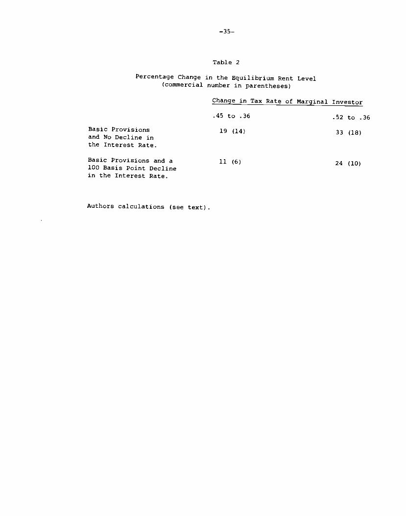
Estimates of the likely rent increase are presented in Table 2 for alternative
of assumptions regarding the tax rate of the marginal investor in real estate
and the size of the interest rate decline.The first numbers, which are
discussed first, are for residential properties; the second numbers (in
parentheses) are for commercial properties.
The top row indicates the equilibrium increase in rent assuming no change
in interest rates for two differentassumptions regarding the tax rate of the
marginal investor under prel9s6 law. With a 45 percent marginal tax rate,
rents will increase by 19 percent; witha 52 percent marginal rate, the rent
increase is 33 percent. These increasesare partially a result of increases in
the required rate of return (81 and 182basis points, respectively, for the 45
and 52 percent tax—bracket investors) owing to the generally lighter taxation
of pretax returns on alternative investments.Because ample evidence exists
that taxpayers with tax rates far below the maximum are active in the rental
market, the 19 percent increase seems more plausible than the 33 percent
increase.

—17—
In the second row a 100 basis point decline in interest rates (and a 68
basis point decline —— relative to that incorporated in the first row —— in the
required after—tax equity rate) is factored into the analysis. The result is a
substantial reduction in the required rent increase: from 19 percent to 11
percent for the 45 percent tax—rate investor and from 33 percent to 24 percent
for the 52 percent investor. The rational for believing that the Tax Act would
lower interest rates was developed earlier.
The required return on equity in real estate could rise relative to that
on other investments because the importance of the relatively certain tax
depreciation component of the return to real estate will decline vis—a—vis the
less certain net—operating—income component. Moreover, real—estate losses will
no longer be deductible against nonpassive income. If one's passive activities
should fall on hard times, the lack of deductibility against other income would
result in the investor shouldering the entire loss, as opposed to sharing it
with the U.S. Treasury. A one percent increase in the required return would
raise all equilibrium rent increases in Table 2 by about four percentage
points.
Our own view is that a 10 to 15 percent rent increase for residential
properties is most likely. That is, we believe (1) the marginal investor under
the old law to have been in the 45 percent tax bracket, (2) the likely decline
in interest rates to be 100 basis points, and (3) some increase in the required
return to be necessary to offset the increased riskiness of real estate
investments.
The rent increases for commercial properties —— the numbers in
parenthesis in Table 2 —— are lower. For the 45 percent tax rate, the
percentage increases are about 5 points less; for the 52 percent tax rate, the
increases are 7 points less. While tax depreciation for commercial properties
is less generous than for residential under the new law, depreciation for the
—18—
former was even less generous than for the latter under the old law. For
commercial properties, then, the expected range of "rent" increases is S to 10
percent.
It is important to reiterate the process by which rents increase in
competitive markets. Builders will find it less profitable to invest at the
current level of rents with the new tax incentives than with the old. The
combination of reduced new construction with normal growth in demand and steady
obsolescence of the existing stock will eventually generate higher rents for
the existing stock.
How quickly will rents rise from the old equilibrium level to the new?
The rise will occur at the mostrapid rate in fast—growing markets and will get
to the new equilibrium sooner the smaller the change in the equilibrium level.
Of course, in markets with high vacancy rates this rent rise will occur only
after current rents and occupancy rates get back to their equilibrium level
under old law. Our best guess is that it willtake four (Columbus, Ohio) to
ten (Houston, Texas) years for rents to rise to their new equilibrium level.
Which provisions of the Act are most responsible for the rent increases?
Estimates of the effects of the individualprovisions, including a change in
the marginal tax rate from 0.45 to 0.36, were computed two ways: the change
in the equilibrium rent if a specificprovision were the only change being made
and the change when this provision is added after all other provisions ——
including a 100 basis point decline in the rate of interest —— had been taken
into account. Either way, the depreciation change increases rents about twice
as much as the cut in the regular income taxrate does, and the impacts of the
CPIT and capital gains exclusion are negligible. Removal of the capital gains
exclusion is of little importance because(1) few gains are expected in a low
inflation enviromnent, (2) gains are expected to be realized in the far distant
—19—
future (see the next paragraph), and (3) the gains exclusion is also removed on
alternative investments, a fact that will lower the required return on real
estate and thus tend to offset the direct impact of the exclusion removal.
Trading should decrease under the new law. Under old law, trading before
tax depreciation disappeared in the 19th year was advantageous. Trading should
not be optimal prior to the new 27½ (or 31½) year tax depreciation life because
a penalty to trading —— the capital gains tax rate —— has been increased and an
advantage to trading —— getting on the new depreciation schedule —— has been
decreased (see Hendershott and Ling, 1984, on optimal trading). Moreover, the
value of installment sale transactions, a method of dampening the capital—gains
tax penalty, is greatly reduced in the Tax Act for sales of assets worth over
$150,000 for sellers with substantial debt. In effect, the fraction of taxes
that could formerly be deferred is reduced by the ratio of the seller's debt to
book value of assets.
B. Impact on the Value of Existing Properties
We now turn to the short—run impact of the Act upon the value of existing
real estate. The initial perspective taken is that of an investor in early
1987 contemplating purchase of property put in place in 1986. This new
investor will face a less generous tax depreciation schedule, a higher capital
gains tax rate, a lower marginal tax rate and, possibly, passive loss
limitations. The question, then, is how much will this new investor alter his
bid for the property relative to his bid under previous law? The standard of
comparison is the price of the property that would have made it a zero net
present value investment under the old law, assuming that rents were at their
equilibrium level.
If rent instantaneously jumped to its new equilibrium level, then value
would not decline; the higher rent would compensate exactly for the less
generous tax depreciation, lower marginal tax rates, etc. Because rent will
—20—
not rise instantaneously, value will decline, the magnitude depending on how
Slowly investors think rent will rise to the new equilibrium level (Hendershott
and Ling, 1985) . The longer is the expected adjustment —— the greater is the
present value of expected below equilibrium rents —— the greater will be the
fall in value. A useful analogy can be drawn to the pricing of discount bonds.
Bonds sell at a discount when they are earning a below—market coupon (rent)
The more the coupon is below market and the longer the bonds are expected to
earn the below—market coupon (the longer is the bond's maturity), the lower is
the market value relative to par.
Investor expectations of the rental adjustment process should vary with
both the growth rate of the area and the extent of initial disequilibrium. We
consider two growth rates (zero and positive) and three prereform states of the
market (equilibrium, 10 percent "excess capacity" and 20 percent excess
capacity) . In all cases, depreciation or obsolescence is assumed to occur at
the rate of 2 percent per year. Thus 10 percent excess capacity or below
market rent would be eliminated in 5 years even with zero growth. The positive
growth market is assumed to eliminate 5 percentexcess capacity per year, 2 for
obsolescence and 3 for growth. Thus 30percent initially below—market rents,
20 percent due to excess capacity and 10 percent due to tax reform, would be
eliminated in 6 years in the high growth area versus 15 years in the no—growth
area.
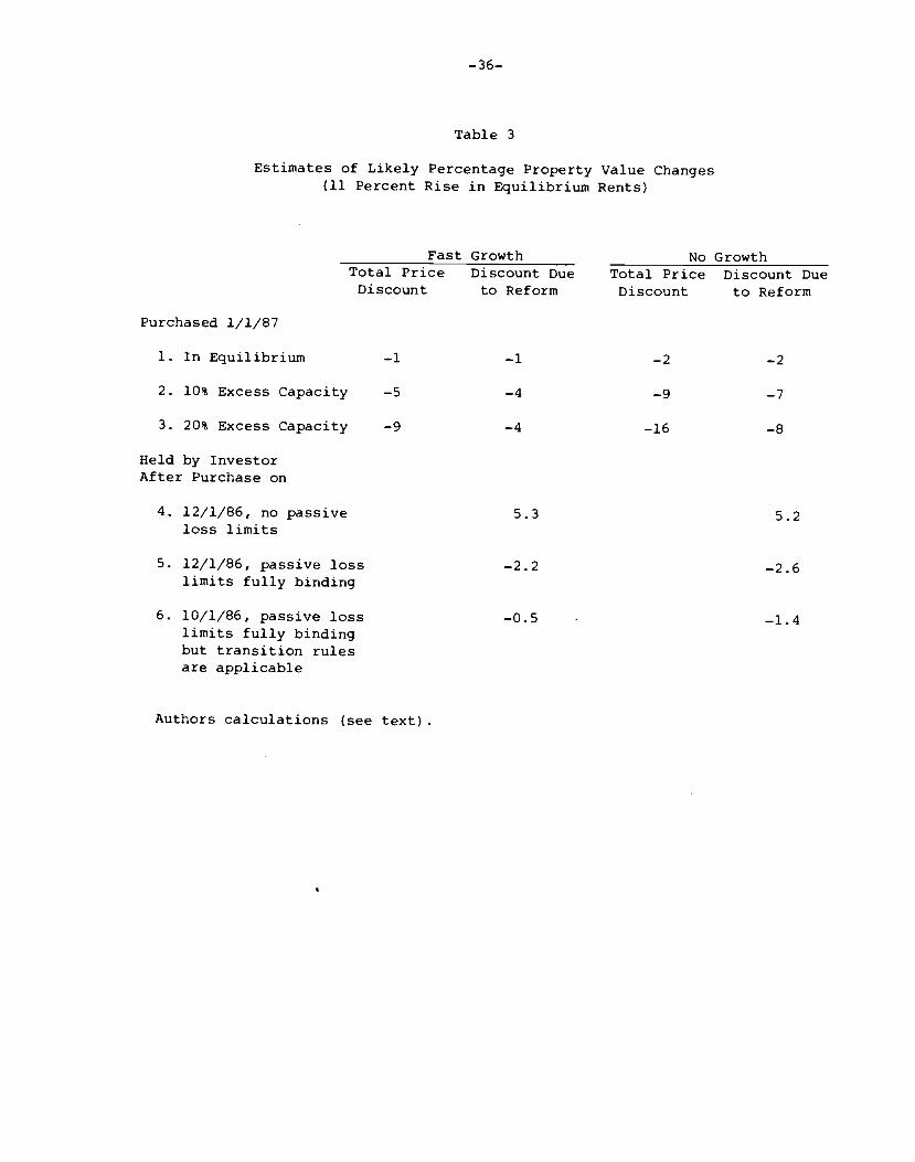
The upper half of Table 3 contains estimates of the percentage value
declines in a property purchased in early 1987 owing to an 11 percent increase
in equilibrium rents and the failure of actual rents to increase immediately to
that level. The first row is for a property that would have had a zero net
present value under the old law, i.e., is in a market in equilibrium prior, to
the enactment of the Tax Act. As can be seen, the value decline is a modest
one percent in a growth market and two percent in a no—growth market.
—21—
Rowe 2 and 3 pertain to cases of 10 and 20 percent excess capacity. In
these calculations, we first compute the total percentage price discount from
reproduction cost and then attribute some of it to the initial disequilibrium
and the remainder to tax reform. The calculations are illustrated in Figure 2
which plots real rent over time. The solid horizontal line is equilibrium real
rent in the absence of tax reform; the dashed horizontal line is equilibrium
rent with tax reform. Now consider a market initially in equilibrium. As a
result of tax reform at time 0 in the figure, rent rises along the BC segment,
the slope of which is steeper in growth areas than in no—growth areas. The
decline in value is measured as the ratio of the present value of triangle ABC
to the initial value (reproduction cost) . Next, consider a market with
substantial excess capacity prior to enactment of the Tax Act, i.e., initial
rent equal to p rather than B With passage of the Act, rent rises along the OF
segment. The percentage price discount from reproduction cost is the ratio of
the present value of triangle ADF to reproduction tost. The percentage decline
in value due to the Tax Act is then the ratio of the difference in the present
values of ADF and HOE —— the present value of ABEF —— to the initial below
market price (reproduction cost less the present value of triangle HOE)
As can be seen in Table 3, the value declines are far larger when
substantial excess capacity exists. The Tax Act is seen to reduce value, from
an already depressed level, by 7 or 8 percent in no—growth areas versus only 4
percent in a growth area. The 8 percent is probably the upper bound on value
decline. The 11 percent rent increase and 20 percent excess capacity is a
worse case commercial scenario and is probably equivalent to a worst case
rental scenario. While greater rent increases are possible for rental, excess
capacity is far less.

—21a—
Figure 2Rent Paths with and without the Tax Act
C F New Equilibrium
___________________________________Old Equilibrium
Time
—22—
The perspective taken above was that of new buyer of the property in
early 1987; an alternative perspective is that of the current owner of a new
property placed in service in 1986. The value of the investment to this person
will exceed that to the 1987 purchaser because this person will be able to use
the more generous tax depreciation schedule from previous law and, if he
purchased before 10/22/86, the passive loss transition rules. The computations
are contained in the lower half of Table 3. Note that the value to this
investor rises even if rents are expected to take 5 years to adjust (the no
growth assumption), as long as the passive loss limits are not binding. That
is, the present value of the tax saving from the more favorable tax
depreciation exceeds the present value of the below—market rents. However, if
the investor has no passive income to offset passive losses and is not eligible
for the transition rules (row 5), the more generous depreciation is of no
value. Because this investor is worse off than the marginal investor, who is
not affected by the passive loss limits by assumption, value declines are
greater than those in row 1. Finally, if this investor purchased the property
before 10/22/86 (row 6), the value declines would be less than those of the
marginal investor purchasing in 1987. That is, the transition rules would
nearly allow the investor to maintain value.
A comparison of row 1 with rows 4—6 yields interesting implications
regarding trading in 1987. Row 1 can be viewed as the maximum bid price,
relative to reproduction cost, of an investor for a property in 1987 whereas
rows 4—6 give the relative value to owners of the property in different tax
situations. An owner will sell only if the bid price of a new investor exceeds
the value of holding the property. These numbers suggest (1) a strong
disincentive by owners not subject to the passive loss limits to trade
properties purchased in 1986, (2) a mild disincentive for owners subject to the
limits but eligible for the transition rules, and (3) a strong incentive to

—23—
trade by those subject to the limits and not eligible for the transition rules.
In fact, the latter investor trades in the first or second period in our model
to maximize his return (minimize his loss). A disincentive to trade also holds
for investors not subject to the loss limits who purchased properties in
earlier years, but the disincentive is less the earlier the property was
purchased because the present value of the tax saving from the more generous
depreciation under old law is less.
IV. Impact on Owner—Occupied Housing
Current law grants important benefits to homeowners: imputed rental
income is not taxed, and capital gains are rarely taxed and then only on a much
deferred basis. Moreover, the deductibility of home mortgage interest ensures
that itemizing households who debt finance will benefit fully from the
nontaxation of owner—occupied housing. A consequence of these favorable
provisions is that homeowners receive substantial tax subsidies. The higher
the marginal tax rate of an individual, the larger the subsidy and the lower is
the after—tax cost of owner—occupied housing.
The Tax Act of 1986 does not directly alter any of these favorable
provisions, but it does affect the after—tax cost ofowner—occupied housing.
First, the tax rates at which households deduct housing costs are reduced.
Second, the pretax level of interest rates will be lower. Furthermore, the
combination of changes in owner costs and in market rents will likely change
the aggregate homeownership rate.
The annual after—tax cost of obtaining one unit of housing capital
depends upon the cost of debt, the cost of contributedequity, property taxes,
real economic depreciation, expected appreciation, and the tax savings
associated with owner—occupied housing. Two costs or "prices" of owner housing
are relevant: the average cost, which influences the tenure choice decision;
—24—
and the marginal cost, which affects the quantity demanded by households that
choose to own. The average and marginal costs, respectively, are higher the
lower are the average and marginal tax rates at which housing costs are
deductible.
Estimates of owner housing costs for households in different income
classes under both old law and the Tax Act are contained in Table 4, based on
the tax rates listed in Table i.8 If interest rates were not affected by the
Tax Act, then the marginal cost would be unchanged for households with incomes
under $30,000 but would rise by roughly 10 percent for those with higher
incomes because of the general decrease in the tax rates at which marginal
housing costs are deducted. If, however, interest rates decline by 100 basis
points, as we expect, then households with incomes below about $30,000 will
experience about a ten percent decrease in marginal housing costs, households
with incomes above about $130,000 will face a 5 percent increase, and the
change for other households will be negligible. Thus any tendency toward
softer house prices will be confined to only the very high end of the market
(over $250,000) and will be modest in magnitude.
In the absence of a decline in interest rates, average housing costs
increase 5 to 10 percent across the board. Costs increase for households with
incomes below $30,000, in spite of roughly no change in marginal tax rates,
because the Tax Act both raises the standard deduction and reduces nonhousing—
related itemized deductions (sales taxes, consumer interest, etc.), causing
more housing deductions of these households to be wasted than was the case
under the old law. With the 100 basis point decline in interest rates,
however, average housing costs will decrease slightly for households with
incomes below approximately $60,000; households with incomes above about
$120,000 will experience a 5 percent increase in costs.
—25—
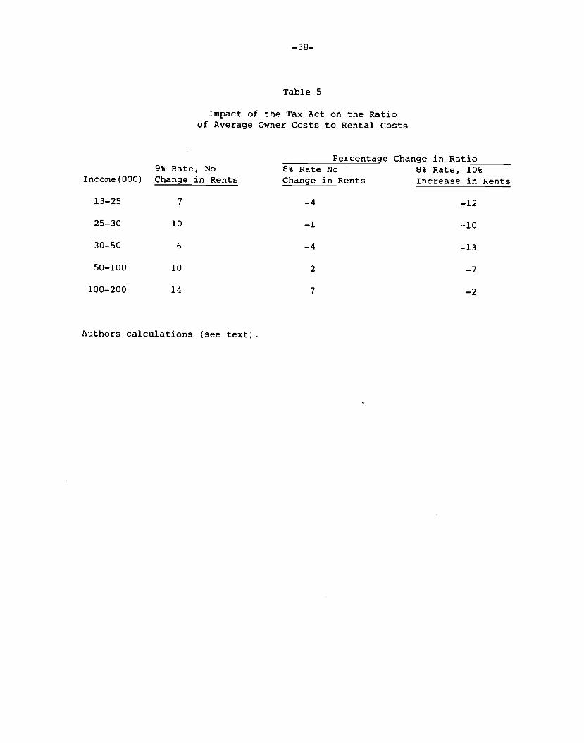
Homeownership depends on, among other things, the ratio of the average
cost of owning to the cost of renting. The percentage changes in these ratios
for households in the various income classes are reported in Table 5. The
calculations in column 1 assume no decline in interest rates and no change in
rents. Columns 2 and 3 factor in the 100 basis point decline in interest
rates, first without, then with, a 10 percent increase in rental costs.
Because rents are held constant in columns 1 and 2, the percentage changes
equal the percentage changes in average owner costs for each income level.
With the interest rate decline and no rent increase, the ownership rate will
likely increase modestly for households with incomes below about $60,000 and
decrease ever so slightly for higher income households. With the rise in
rents, all currently renting households will find homeownership relatively more
attractive than under old law. Overall, theaggregate homeownership rate would
eventually rise by about 3 percentage points.
V. Low—Income Rental Housing
Tax incentives to stimulate the construction of low—income rental housing
have been part of the law for many years. Previous law allowed investors in
low—income properties to depreciate the properties over 15 years and to use a
200 percent declining balance method; in addition, CPIT would be expensed
during the construction period. Furthermore, investors often had access to
tax—exempt financing at rates substantially below market.
The Tax Act changes this law in two important respects. First, the
preferential depreciation and construction period write—off schedules are
replaced with a system of tax credits that depends upon the type of housing
purchased or built and whether the project has access to tax—exempt financing
or other types of subsidy. Specifically, the investor receives:
—26—
1) An annual credit for 10 years which has a present value equal to 70
percent of the cost of construction (both new and substantially
rehabilitated projects) placed in service between 1/1/87 and
12/31/89. For 1987, the applicable Treasury discount rate converts
into a 9 percent annual credit, but this credit will rise if interest
rates rise and fall if rates decline.
2) For existing low—income housing or new construction with tax—exempt
financing or other rental housing subsidies (e.g., FmHA section 515
loans), the present value of the credit is 30 percent (the annual
credit for 1987 is 4 percent)
The depreciable basis is not reduced by the credit. Second, the availability
of tax—exempt financing is reduced.
An analogy to the passive loss limits applies to these credits, as does a
"small landlord provision." The latter says that up to $7,000 in credits (0.28
times $25,000) can be used to offset taxes on regular or portfolio income by
households with taxable income below $200,000 (no active management criterion
need be met) . The offset is phased out between $200,000 and $250,000. With a
nine percent annual credit, an investment of up to $77,778 ($7,000/.09) is
eligible for the full offset.
Potentially severe restrictions are placed upon investments to qualify
investors for the credits. First, at least 20 (40) percent of the units must
be occupied by tenants whose income cannot exceed 50 (60) percent of the area's
median income adjusted for family size, and only the units so occupied receive
the credit. (Previous law defined qualifying income as 80 percent of the
area's median income.) Second, tenants cannot pay more than 30 percent of
their income in rent. Third, the project must satisfy these
—27—
15 years after it is placed in service or purchased, otherwise a substantial
penalty will be levied. Fourth, the total value of the credits issued in a
state is limited to $1.25 times of the population of the state.
A number of difficult conceptual problems exist in modeling low—income
housing. These include specifying the expected sales prices at year 15 and
beyond and the depreciation rates and required equity returns, both which are
presumably higher than their counterparts for regular rental housing. These
and other problems must be addressed before a definitive statement can be made
on the treatment of low—income housing in the Tax Act vis—a—vis old law.
Nonetheless, we have made a few "minimum" rent calculations that are probably
instructive.
The minimum rent required by investors to earn their required rate of
return is half as large with the new 9 percent credit as it was under old law,
even when tax—exempt financing was employed (the debt rate was 200 basis points
below market). With the 4 percent credit andtax—exempt financing, the minimum
rent is roughly the same as under old law with tax exempt financing. This
suggests two things. First, the 9 percent credit dominates the 4 percent
credit with tax—exempt financing. Thus, limits on tax—exempt financing for
low—income housing may not be of importance. Second, the 9 percent credit is
far more generous than old law. Whether the credit is sufficient to generate a
substantial increase in the construction of low—incomehousing is unknown,
however.
—28—
VI. Summary
In contrast to the conventional wisdom, real estate activity in the
aggregate is not disfavored by the 1986 Tax Act. Within the broad real estate
aggregate, however, widely different impacts are to be expected. Regular
rental and commercial activity will be slightly disfavored (modest increases in
rents and declines in values will occur) , and historic and old rehabilitation
activity will be greatly disfavored. In contrast, owner—occupied housing, far
and away the largest component of real estate, is favored, both directly by an
interest rate decline and indirectly owing to the increase in rents.
Homeownership should rise significantly, and the quantity and value of houses
should increase slightly, except at the very high end of the market. Low—
income rental housing may be the most favored of all activities.
The rent increase for residential properties will be 10 to 15 percent
with our assumption of a percentage point decline in interest rates. For
commercial properties, the expected rent increase is 5 to 10 percent. The
market value decline, which will be greater the longer and further investors
think rents will be below the new equilibrium, is unlikely to exceed 4 percent
in fast growth markets, even if substantial excess capacity currently exists.
Moreover, the value of recently—purchased properties to their current holders
not subject to the passive loss limits will generally rise because the more
generous tax depreciation allowances under old law vis—a—vis new law adds more
value than the expected below—market rent subtracts. In no—growth markets with
substantial excess capacity, market values could decline by as much as 8
percent from already depressed levels.
Two offsetting factors operate on the after—tax cost of owner—occupied
housing. Lower tax rates increase the cost, but lower interest rates decrease
it. With a percentage—point interest—rate decline, the after—tax marginal cost
will fall by about 10 percent for most households with incomes below $30,000
—29—
and rise by about 5 percent for those with incomes above $130,000. Thus, Only
the highest price houses would experience weakness in value. Average housing
costs will decrease slightly in this scenario for households with incomes below
about $60,000, but increase by 5 percent for those with incomes above twice
this level. With the projected increase inrents, homeownership should rise
for all income classes, but especially for those with income under $60,000.
The aggregate home ownership rate is projected to increase by three percentage
points in the long run in response to the Tax Act.
The new passive loss limitations are likely to lower significantly the
values of loss—motivated partnership deals and of properties in areas where the
economics have turned sour (vacancy rates have risen sharply). The limitations
should have little impact on new construction and market rents, however.
Reduced depreciation write—offs, lower interest rates, and higher rents all act
to lower expected passive losses. Moreover, financing can be restructured to
include equity—kickers or less debt generally at little loss of value.
—30-.
Footnotes
This is not the first tax act whose impact on real estate would be
misunderstood without allowing for interest rate changes. Many (Brueggeman,
et. al., 1981, for example) predicted substantial rent decreases in response to
the more generous tax depreciation allowances contained in the Economic
Recovery Tax Act of 1981. Hendershott and shilling (1982)• however, foresaw a
sharp increase in interest rates as a result of the Act and forecast rising
real rents. Real rents have, in fact, risen by 10 percent since 1980.
2The households for which calculations are reported are also assumed to have
one wage earner and the average fringe benefits and nonhousing itemized
deductions of their income classes (based on 1983 SOl data), to own houses of
dollar value equal to twice their AGIs and to pay property taxes equal to 1.2
percent of their house values. The general methodology for computing these tax
rates is discussed in Hendershott and Slemrod (1983).
These credits are subject to the same passive loss treatment as is the credit
for low—income rental housing (see Section IV below).
See Graetz and Sunley (1986) for a detailed discussion of both the individual
and corporate minimum taxes.
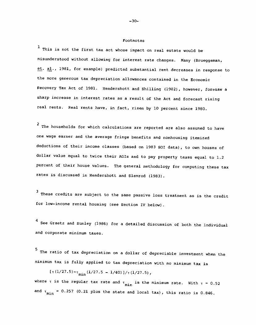
The ratio of tax depreciation on a dollar of depreciable investment when the
minimum tax is fully applied to tax depreciation with no minimum tax is
N /27STmin(1275 — 1/40) ]/t (1/27.5),
where T is the regular tax rate and t is the minimum rate. With t = 0.52mi n
and T = 0.257 (0.21 plus the state and local tax) , this ratio is 0.846.mm
—31—
6A potential problem with discounted cash flow models of this type is
consistency between the assumed patterns of future rents and prices (Ling and
Whinihan, 1985) Assuming that rents are initially at the equilibrium level,
the 2½ and 3 percent assumed depreciationrates provide consistency, e.g., the
resale price at year 20 is within one percent of the present value of cash
flows beyond year 20. This consistency holds for both old law and the Tax Act.
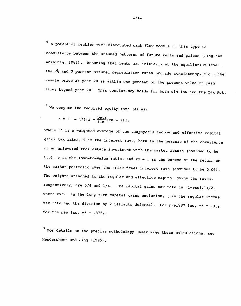
We compute the required equity rate Ce) as:
e = (1 — t*)[i + beta( — i)],where t is a weighted average of the taxpayer's income and effective capital
gains tax rates, i is the interest rate, beta is the measure of the covariance
of an unlevered real estate investment withthe market return (assumed to be
0.5), v is the loan—to—value ratio, and rm — i is the excess of the return on
the market portfolio over the (risk free) interest rate (assumed to be 0.06)
The weights attached to the regular and effectivecapital gains tax rates,
respectively, are 3/4 and 1/4. The capital gains tax rate is (l—excl.)1/2,
where excl. is the long—term capital gainsexclusion, t is the regular income
tax rate and the division by 2 reflects deferral.For prel987 law, t* =
for the new law, * = .87S.
For details on the precise methodologyunderlying these calculations, see
Hendershott and Ling (1986).
—32—
Ref erences
Brueggeman, William B., Jeffrey D. Fisher and Jerrold J. Stern, "Rental Housing
and the Economic Recovery Tax Act of 1981," Public Finance Quarterly, 10, April
1982, pp. 222—241.
Galper, Harvey, Robert Lucke and Eric Toder, "The Economic Effects of the Tax
Reform Act of 1986: Simulations with a General Equilibrium Model," Brookings
Tax Conference, October 30—31, 1986.
Graetz, Michael J. and Emil Sunley, "Minimum Taxes and Comprehensive Tax
Reform," Brookings Tax Conference, October 30—31, 1986.
Hendershott, Patric H., "Tax Changes and Capital Allocation in the 1980s," in
Feldstein (ed.), The Effects of Taxation on Capital Formation, University of
Chicago Press, 1987.
Hendershott, Patric H. and David C. Ling, 1984, "Trading and the Tax Shelter
Value of Depreciable Real Estate," National Tax Journal, June 1984, pp. 213—
223.
Hendershott, Patric H. and David C. Ling, 1985, "Prospective Changes in Tax Law
and the Value of Depreciable Real Estate," Journal of the American Real Estate
and Urban Economics Association, Fall 1984, pp. 297—317.
Hendershott, Patric H. and David C. Ling, 1986, "Likely Impacts of the
Administration Proposal and the House Bill," in Follain (ed.), Tax Reform and
Real Estate, The Urban Institute, 1986, pp. 87—112.
—33—.
Hendershott, Patric H. and James Shilling, "The Impacts on Capital Allocation
of Some Aspects of the Economic Recovery Tax Act of 1981," Public Finance
Quarterly, April 1982, pp. 242—273.
Hendershott, Patric H. and Joel Slemrod," "Taxes and the User Cost of Capital
for Owner—Occupied Housing," Journal of the An1erican Real Estate and Urban
Economics Association, Winter 1983, pp. 375—393.
Ling, David C. and Michael Whinihan, "Valuing Depreciable Real Estate: A New
Methodology," Journal of the American Real Estate and Urban Economics
Association, Summer 1985, pp. 181—194.

—34—
Table 1
Tax Rate at Which Housing Costs Are Deductible
Tenure Choice (Average) Quantity Demanded (Marginal)
Income (000) Old Law Tax Reform Old Law Tax Reform
13—25 .146 .074 .166 .176
25—30 .211 .128 .189 .180
30—50 .279 .242 .251 .184
50—100 .402 .316 .364 .316
100—200 .471 .370 .455 .370
Authors calculations (see footnote 2).
—35—
Table 2
Percentage Change in the Equilibrium Rent Level(commercial number in parentheses)
Change in Tax Rate of Marginal Investor
.45 to .36 .52 to .36
Basic Provisions 19 (14) 33 (18)and No Decline inthe Interest Rate.
Basic Provisions and a 11 (6) 24 (10)100 Basis Point Declinein the Interest Rate.
Authors calculations (see text).
—36—
Table 3
Estimates of Likely Percentage Property Value Changes(11 Percent Rise in Equilibrium Rents)
Fast Growth No GrowthTotal Price Discount Due Total Price Discount DueDiscount to Reform Discount to Reform
Purchased 1/1/87
1. In Equilibrium —l —l —2 —2
2. 10% Excess Capacity —5 —4 —9 —7
3. 20% Excess Capacity —9 —4 —16 —8
Held by InvestorAfter Purchase on
4. 12/1/86, no passive 5.3 5.2loss limits
5. 12/1/86, passive loss —2.2 —2.6limits fully binding
6. 10/1/86, passive loss —0.5 —1.4limits fully bindingbut transition rulesare applicable
Authors calculations (see text)

—37—
Table 4
Marginal and Average After—Tax Cost ofOwner—Occupied Housing by Income Class
Tax Act of 1986Old Law 9% Interest Rate 8% Interest Rate
Income(000) Marg. Ave. Marg. Ave. Marg. Ave.
13—25 .0818 .0851 .0808 .0909 .0729 .0820
25—30 .0795 .0777 .0804 .0865 .0726 .0772
30—50 .0734 .0700 .0800 .0743 .0722 .0673
50—100 .0633 .0610 .0670 .0670 .0624 .0624
100—200 .0567 .0550 .0629 .0629 .0588 .0588
Authors calculations (see footnote 2).
—38.-.
Table 5
Impact of the Tax Act on the Ratioof Average Owner Costs to Rental Costs
Percentage Change in Ratio9% Rate, No 8% Rate No 8% Rate, 10%
Income(000) Change in Rents Change in Rents Increase in Rents
13—25 7 —4 —12
25—30 10 —1 —10
30—50 6 —4 —13
50—100 10 2 —7
100—200 14 7 —2
Authors calculations (see text)