NBER WORKING PAPER SERIES

INTERNATIONAL R&D SPILLOVERSBETWEEN U.S. AND JAPANESE

R&D INTENSIVE SECTORS

Jeffrey L BernsteinPierre Mohnen

Working Paper No. 4682

NATIONAL BUREAU OF ECONOMIC RESEARCH1050 Massachusetts Avenue

Cambridge, MA 02138March 1994

The authors would like to thank Ned Nadiri, Zvi Griliches, and Dale Jorgenson for helpfulcomments and support. Financial support from the Canadian Social Sciences and HumanitiesResearch Council is gratefully acknowledged. This paper is part of NBER's research programin Productivity. Any opinions expressed are those of the authors and not those of theNational Bureau of Economic Research.

NBER Working Paper #4682March 1994

INTERNATIONAL R&D SPILLOVERSBETWEEN U.S. AND JAPANESE

R&D INTENSIVE SECTORS

ABSTRACT

A great deal of empirical evidence shows that a country's production structure and

productivity growth depend on its own R&D capital formation. With the growing role of

international trade, foreign investment and international knowledge diffusion, domestic production

and productivity also depend on the R&D activities of other countries. The purpose of this paper

is to empirically investigate the bilateral link between the U.S. and Japanese economies in terms

of how R&D capital formation in one country affects the production structure, physical and R&D

capital accumulation, and productivity growth in the other country.

We find that production processes become less labor intensive as international R&D

spillovers grow. In the short-run, R&D intensity is complementary to the international spillover.

This relationship persists in the long-run for the U.S., but the Japanese decrease their own R&D

intensity. U.S. R&D capital accounts for 60% of Japanese total factor productivity growth, while

Japanese R&D capital contributes 20% to U.S. productivity gains. International spillovers cause

social rates of return to be about four times the private returns.

Jeffrey L Bernstein Pierre MohnenDepartment of Economics Department of EconomicsCarleton University University of Quebec at MontrealOttawa, Ontario K1S 5B6 Montreal, Quebec H3C 3P8CANADA CANADAand NBER

1. tntroduction*

A wealth of evidence suggests that a country's production process and

productivity growth depend on its current and past investments in R&D

activities (see the surveys by Griliches (1988], and Nadiri (1993)).

Moreover, with the growing importance of international trade in products and

services, foreign direct investment, and international knowledge diffusion, a

country's production structure and productivity growth depend, not only on

the accumulation of its own R&D capital, but also on the R&D activities of

other economies.1 The purpose of this paper is to empirically investigate

how U.S. R&D capital accumulation affects the production structure, physical

and R&D capital formation, and productivity growth in the Japanese economy,

and simultaneously how Japanese R&D investment affects these same elements in

the U.S. economy.

There is a public good aspect to R&D capital accumulation. The benefits

from R&D cannot be be completely appropriated by the R&D performers, and,

inevitably, there are spillovers or externalities. R&D spillovers spur the

diffusion of new knowledge, while they simultaneously create disincentives to

undertake R&D investment. A number of recent empirical papers have shown the

importance of domestic R&D spillovers in generating productivity gains and in

affecting R&D capital accumulation (see the surveys by Griliches (1988),

Cohen and Levin (1989], and Nadiri [19933)

* The authors would like to thank Ned Nad.iri, Zvi Griliches, and DaleJorgenson for helpful comments and support. Financial support from theCanadian Social Sciences and Humanities Research Council is gratefully

acknowledged.

—2—

R&D spillovers are not necessarily contained within national boundaries.

International R&D spillovers are transmitted in a number of ways. Exports of

goods and services, international alliances between firms, such as licensing

agreements and joint ventures, foreign direct investment, international

labor markets for scientists and engineers, and international

communications, such as conferences, are some of the transmission mechanisms.

It is important to emphasize that international transactions do not have to

occur in order for spillovers to flow between nations. For example, Japanese

automobile producers operating in the U.S. can perform reverse engineering on

U.S. vehicles in the U.S. and transmit this information back to Japan. Thus

the potential magnitude and extent of international spillovers can be quite

pervasive.

In this paper we develop a bilateral model of production between the

U.S. and Japanese economies (see Jorgenson and Nishintizu [1978], and

Jorgenson, Sakuramoto, Yoshioka, and Kuroda [1990]). The significance of

this approach is that production and R&D decisions for the U.S. and Japan are

modeled simultaneously. International spillovers do not influence only

productivity growth or production cost, but they simultaneously alter

production structures, including decisions on R&D capital. Thus we estimate

the effects of international R&D spillovers on production cost, traditional

factor demands (such as the demand for labor), the demand for R&D capital,

and productivity growth rates in each country.

We generalize the bilateral production model to account for adjustment

costs associated with physical and R&D capital formation. Empirical evidence

—3—

3uggests that adjustment costs prevent producers from iwtnediately attaining

long—run equilibrium Csee Morrison and Berndt (1981), Epstein and Yatchew

(1985), Mobnen, Nadiri and Prucha (l986J, and Bernstein and Nadiri (1989)).

Producers adjust toward long—run equilibrium through successive short—run or

temporary equilibria. Thus we are able to determine the bilateral effects on

cost and production structure associated with international spillovers

between the U.S. and Japanese economies in both the short and long—runs.

Moreover, Berndt and Fuss [1986, Mohnen and Bernstein (1991], and Morrison

(1992) have shown that it is important to account for deviations from

long—run equilibrium in measuring productivity growth. Mistakenly assuming

that producers are at their long—run desired capital stock levels (both for

physical and R&D capital) can lead to significant biases in measured

productivity growth rates and biases in accounting for the various

determinants of productivity growth. In this paper we investigate the

contribution to productivity growth from international spiliovers within the

context of adjustment costs for physical and R&D capital accumulation.

This paper is organized into a number of sections. The next section

contains the specification of the model. Section 3 presents the estimation

results, results from various hypothesis tests, and measures of adjustment

costs. The international spillover effects in both the short and long—runs

are described in section 4. The contribution of international spillovers to

productivity growth and to the social rates of return are presented in

section 5. In the last section we conclude the paper.

—4—

2. Modal Specification

The model that we specify enables us to investigate the effects of

Japanese R&D capital on the production structure in the U.S., and conversely

the effects of U.S. R&D capital on Japanese production. Specifically, we

want to determine the effects of one country's R&D capital on cost, factor

demands, capital accumulation, and productivity growth in the other country.

Production process in each country can be represented by,2

Cl) F(v,K,4K,5)

where y is output, v is the n dimensional vector of variable factor demands,

K is the m dimensional vector of quasi—fixed or capital factor demands, S is

the o dimensional vector of R&D spillovers, which in a bilateral production

model is the R&D capital from the other country, F is the production

function,3 In the production function the presence of AX — —

signifies that there are adjustment costs associated with changes in the

capital inputs.

The capital inputs accumulate according to,

(2) 1< — I + CI —t t In t—l

where I is the vector of gross additions to the capital inputs, I is the m

dimensional identity matrix, (as there are in capital inputs), and 6 is the

—5—

diagonal matrix of constant depreciation rates.

Production decisions in each country are determined under

competitive conditions and according to the minimization of the expected

discounted stream of costs. Thus,

T T(3) man E(EQ a(O,r)(wv +

{v ,It .r t—o

where E is the conditional expectations operator in the current period, a is

the discount factor, w is the vector of exogenous variable factor prices, and

q is the vector of exogenous capital acquisition prices. Now (3) is

minimized subject to the production function, (equation (1)), the capital

accumulation conditions, (equation (2)), and the expected stream of output,

variable factor prices and capital acquisition prices. This problem can be

solved in two stages. The first stage pertains to the determination of the

variable factor demands, while the second stage relates to the demands for

the capital inputs. Suppose for the moment that the capital inputs are

given. In order to find the variable factor demands from (3), we minimize at

each point in time wtv subject to the production function and conditional on

the capital inputs. The variable factor demand functions which are obtained

as the solution to this problem are considered the short—run production

equilibrium conditions, because the capital inputs are fixed. Substituting

the short—run equilibrium conditions into variable factor cost (that is wtv)

yields the variable cost function,

—6—

(4) c CV(w,y,K1,AK,s1)

where cV is variable cost and is the variable cost function, which is

twice continuously differentiable, nondecreasing in w, y, and X,

nonincreasing in K, concave and homogeneous of degree one in w, convex in K

and ax.

We specify the following functional form for the variable cost function,

(5) — (aw + .5w'ftwW1 + wØS1)y +

1) T+ .5K' 1Q( W/y + K' 1(S 1W + .SAKMAKW/y

where w — w is an index of variable factor prices, where the coefficient

vector is known and defined by the particular index number.4 The parameters

are represented by the nfl vector a, the nxn matrix $, the nxo matrix 0, the

man matrix , the mxm matrix g, the mxo matrix t, the mxm matrix JS, and the

scalar ij. The parameter matrices are assumed to be symmetric. This

functional form is a simple extension of the one developed by Diewert and

Wales [1997). The extension involves the possibility of non—constant returns

to scale (7) is the inverse of the scale parameter) and adjustment costs (p is

the adjustment cost parameter matrix)) Adjustment costs are such that in

the long run when there is no net investment, marginal adjustment costs are

zero. The functional form incorporates the condition that the variable cost

—7—

function is homogeneous of degree one in variable factor prices. The

attractiveness of this functional form is that the concavity and convexity

properties of the variable cost function can be imposed without restricting

the flexibility of the function. In addition, under suitable expectations cf

the exogenous variables, closed form solutions can be obtained for the

quasi—fixed factors.

The demands for the variable factors are retrieved from the variable

cost function by applying Shephard's Lemma (see Diewert (1982]). Thus with

v — and using

(6) vt — (a + — .swww2v + 0T5 )yfl ..

+ ( .5K 1K 1/yfl + K1(S + .5AXTjthK/y)v.

The variable factor demands depend on the variable factor p;ices, output, the

capital inputs, net investment in the capital inputs and the R&D spillovers.

In order to determine the demands for the capital inputs, substitute the

right side of (5) into (3) for wv and maximize (3) subject to the capital

accumulation equations (given as equation set (2)) . Assuming that relative

variable factor prices Cw/W), output, R&D spillovers and the real discount

rate (a(t,t+l) (1+r)1) are not expected to change, then the demands for

the capital inputs are given by,6

(7) K — + (I — 14)Kt t m t—1

—8—

where H is the adjustment coefficient matrix, and the long—run demands for

the capital inputs are K - — 1A, where A — ('w/W + (S1 +

and w' — Cr1 + is the vector of rental rates for the capital inputs.

The matrix of adjustment coefficients must satisfy the following matrix

equation,

(8) + C + ri)M - — 0.

In general, we cannot solve for H in terms of and p. However, as shown by

Epstein and Yatchew [19851, we are able to solve for in terms of i and H.

Define B — —pM and C — —M(t, where B and C are symmetric matrices. Thus,

using (8), C + (1 + r) (B — rw)1, and the demands for the capital

inputs can be written as,

(9) K CA + (I +t t I' t—1

The demands for the capital inputs are written in terms of the parameter

matrices B and p. Notice that the adjustment coefficient matrix can be

obtained from these parameter matrices, as H — —M'B. The demands for the

capital inputs depend on the lagged values of these inputs, and through the A

matrix, the demands also depend on variable factor prices, the rental rates,

output quantity, and the R&D spillovers.7

The set of equations to be estimated consists of (6) and (9), which

—9—

relate to the demands for the factors of production. Our emphasis in this

paper is on the effects that international R&D spillovers have on production

structure and productivity growth. We see that this framework enables us to

investigate the impact of international R&D spillovers on factor demands in

the short and long runs, as well on the decomposition of productivity growth.

3. Estination Rasults

The data used to estimate the model relate to a common set of industries

and time period for the United States and Japan. There are eleven

industries. These are Food and and Kindred Products, Paper and Allied

Products, Chemicals and Allied Products, Petroleum and Coal Products, Stone

Clay and Glass, Primary Metals, Fabricated Metals, Non—electrical Machinery,

Electrical Products, Transportation Equipment, and Scientific Instruments.

The sample period is 1962—1988. the non—R&D data are described in detail in

Denny, Bernstein, Fuss, Waverman and Nakamura (19921.8 The industries for

each country are aggregated by Fisher indexes (see Diewert. (1989]) into a

single sector. We refer to this sector as the R&D intensive sector as 90% of

all manufacturing R&D investment is performed here.9 the industries are

aggregated into broad R&D sectors because we are interested in the effects

of international spillovers. We want to abstract from the spillovers that

exist between the industries within a country.10

The data consist of prices and quantities for two variable factors,

labor and intermediate; two capital inputs, physical and R&D, output

—10—

quantity, and R&D spillover, which is the R&D capital of the foreign R&D

intensive sector. The data for the Japanese and U.S. R&D intensive sectors

are treated as separate sets of observations. These observations are assumed

to be generated by an econometric model with distinct first order parameters

(represented by the a vector), distinct R&D spillover parameters (represented

by the 0, and ( matrices), distinct scale parameter (represented by the

inverse of ifl, and the remaining second order parameters are common. In this

model differences in the technology across countries at a point in time are

reflected in differences in the a and i parameters. Differences in the

technology over time between the countries are represented by differences in

the spillover parameters (that is by the 0 and ( matrices)

Unobservable stochastic disturbances are added to equation sets (6), and

(9) . These disturbances reflect random elements in the production process

not reflected in the variable cost function, and errors of implementation of

the production plans. The disturbances have zero expected value and

positive definite covariance matrix.'1

Equation sets (6) and (9) were jointly estimated using the nonlinear

Maximum Likelihood Estimator. The first set of estimates produced scale

estimates of 1.004 and 1.021 for the U.S. and Japan respectively. In this

case the log of the likelihood function increased by only 1.329 over the

constant returns to scale model. Thus we could not reject constant returns

to scale for both the U.S. and Japanese R&D intensive sectors.'2 We then

proceeded to estimate the model under constant returns to scale. In

addition, we generalized the flexible accelerator in the following way,

—11-

(10)

where is a two dimensional symmetric parameter matrix, and d is a duimny

variable that takes the value of 1 in short—run equilibrium and 0 in long—run

equilibrium.13 Recall that the M matrix is the adjustment matrix (see

equations (7) and (9)) . If • is zero then the model is consistent with the

flexible accelerator. Equation sets (6) and (9) were estimated under the

hypotheses that 0 — 0 and O 0. Under the null hypothesis the log of the

likelihood function was 484.474 and under the alternative hypothesis the

value was 534.223. Therefore we reject the simple flexible accelerator model

and adopt the generalized form. These estimates are presented in table ,14

In table 1 we see from the squared correlation coefficients, that the model

fits the data quite well.'5 We also estimated the model with only first order

and spillover parameters. In other words we set — — — Mkj 0k —

0, i — l,m, k,j — p,r. In this situation the log of the likelihood function

was 483.219. Thus we reject the absence of second order parameters in the

estimation model. The model was also estimated when the spillover parameters

were set to zero. We set — — 0, 1 — p,r. In this case the log of

the likelihood function was 521.297, and so we reject the model without R&D

spillovers.

In order to see if the U.S. and Japanese sectors are in long—run

equilibrium, the model was estimated under the condition that — 0 , i,j —

p,r. With the three adjustment parameters (since — j2) set to zero the

—12—

Table 1. EstimatiOn Results

Parameter Estimate Standard Error

0.1079 0.7875

cc5 2.4569 1.0472

1.3800 0.7272In

a1 0.9070 0.2164

—0.9150 0.4449

—0.8010E—06 0.1917E—05

—0.4233E—05 0.1266E—05

1p -2.1029 1.4615

1r 3.7565 3.0884

—4.9072 4.4812mp

mr 2.6887 4.5011

b —69.0859 54.0610pp

b 59.1626 88.1947Pr

b —104.4000 101.0550rr

0.2233E—04 0.2269E—04

0.8489E—05 0.8669E—05

C —0.2835E—04 0.2868E—04

—0.8282E—05 0.9111E—05

fL" 323.3500 235.9560

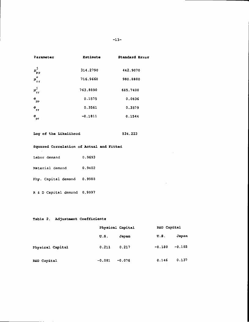
—13—

Parameter Estimate Standard Error

314.2790 442.9070

716.9660 960.8800

763.8890 685.7400

t 0.1575 0.0836pp

• 0.3561 0.3579rr

0 —0.1811 0.1544pr

Log of the Likelihood 534.223

Squared Correlation of Actual and Fitted

Labor demand 0.9693

Material demand 0.9402

Phy. Capital demand 0.9988

R & D Capital demand 0.9997

Table 2. Adjustment Coefficients

Physical Capital R&D Capital

U.S. Japan U.S. Japan

Physical Capital 0.211 0.217 —0.180 —0.185

R&D Capital —0.081 —0.076 0.146 0.137

—14—

log of the likelihood was 409.073. Thus we reject long—run equilibrium for

the R&D intensive sectors of the Japanese and U.S. economies. Indeed, we

can calculate the speeds of adjustment towards long—run equilibrium from

the matrix M — —jiB. The speeds of adjustment are presented in table 2.

This table shows us that the own adjustment speed for physical capital is 45%

faster than for R&D capital in the U.S., while in Japan, physical capital

adjusts 58% faster than R&D capital. Ignoring the cross adjustment

coefficients for the moment, we find in the U.S. that around 21% of the

adjustment for physical capital occurs in the first year. In this same time

period only about 15% of the gap between long and short—run R&D capital stock

closes. For Japan the corresponding speeds are 22% and 14%. The results on

the relative magnitudes of the own adjustment speeds are similar to Mohnen,

ladiri and prucha [19863, for U.S and Japanese manufacturing sectors,

Bernstein and Nadiri [1989] for U.S. firms, and Nadiri and Prucha [1990) for

U.S., and Japanese electrical products industries. However, we find that the

own adjustment speeds for the R&D intensive sectors of the two economies are

faster than for the manufacturing sector as a whole.

The cross adjustment coefficients in table 2 are negative. This means

that physical and R&D capital are adjustment complements. Thus when the

long—run demand for physical capital exceeds the short—run demand the

adjustment of R&D capital decelerates. This same process occurs when the

roles of the two capital stocks are reversed. An excess demand for physical

capital slows the adjustment process of R&D capital by around 18% in a single

year in the U.S. and in Japan. In addition, an excess demand for R&D capital

—15—

slows the physical capital adjustment by 0% in one year in the U.S. and

Japan. In general, we do not find adjustment speeds too dissimilar between

the U.S. and Japanese R&D intensive sectors.

4.- Spiflover Effects

In this section we consider the effects of international R&D spillovers

on the structure of production, We have seen that the estimation model

without international R&D spillovers can be rejected. Thus we want to

calculate the effects of the spillover on variable cost and factor demands.

In particular, we calculate both the short and long—run effects that Japanese

R&D capital exerts on the labor—output, intermediate input—output, physical

capital—output, and R&D capital—output ratios for the U.S. R&D intensivesector, Similarly, we compute the effects for the Japanese R&D intensive

sector based on changes in the U.S. R&D capital.

To determine the short—run spillover effects, differentiate the capital

input demand equations (equation set (9)) with respect to the spillovervariable,

(11) O(K/y)/8S — CC.

Since capital inputs affect the short—run demand for the variable factors

through the capital—output ratio and adjustment costs, differentiating

equation set (6) with respect to the spillover yields,

—16—

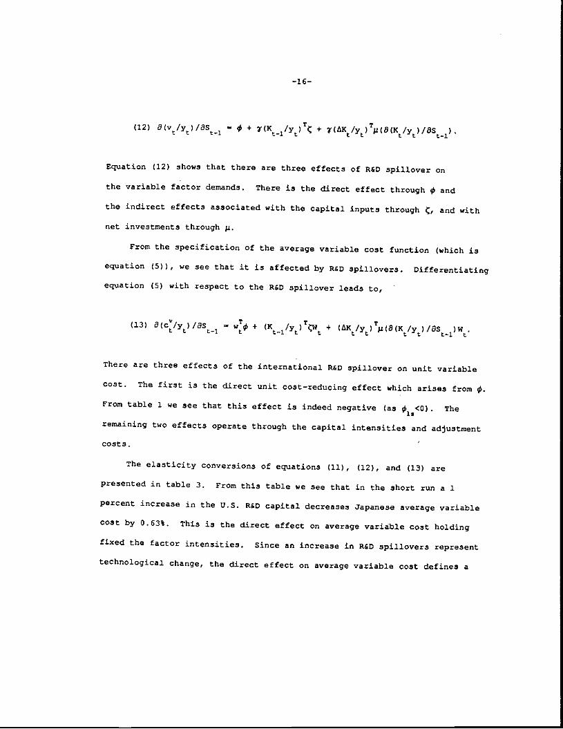
(12) 8(v/y)/88 + CR /y)T( + 7(AK/y)Tj.z(8(K/y)/8s)

Equation (12) shows that there are three effects of R&D spiliover on

the variable factor demands. There is the direct effect through and

the indirect effects associated with the capital inputs through ., and with

net investments through 2.

From the specification of the average variable cost function (which is

equation (5)), we see that it is affected by R&D spillovers. Differentiating

equation (5) with respect to the R&D spillover leads to,

(13) a(c/y)Ias — wT# + (K1/y)TQq + (AK/y)Tg(8(K/y)/3s)w

There are three effects of the international R&D spillover on unit variable

cost. The first is the direct unit cost—reducing effect which arises from0.

From table 1 we see that this effect is indeed negative (as 0<0). The

remaining two effects operate through the capital intensities and adjustment

costs.

The elasticity conversions of equations (11), (12), and (13) are

presented in table 3. From this table we see that in the short run a 1

percent increase in the U.S. R&D capital decreases Japanese average variable

cost by 0.53%. This is the direct effect on average variable cost holding

fixed the factor intensities. Since an increase in R&D spillovers represent

technological change, the direct effect on average variable cost defines a

—17—

Table 3: Short—Run Spiflover Effects

United States Japan

Mean Std. Dey. Mean stu. Dew.

Direct Avg. Vat. Cost —0.0538 0.0273 —0.6334 0.4493

Average Variable Cost 0.2410 0.1857 —0.4260 0.3583

Labor / Output —0.0144 0.0556 —3.5455 1.4255

Inter. Input I Output 0.3158 0.2051 0.3959 0.1385

Phy. Cap. / Output —0.0150 0.0085 0.1301 0.0235

R&D Cap./ Output 0.0255 0.0154 0.0526 0.0068

—18—

measure of the rate of technological change. Thus there are technological

gains for Japan from international spillovers. The U.S. also benefits from

international spillovers. Japanese R&D capital directly reduces U.S.

average variable cost, but the effect is about twelve times smaller than the

spillover effect generated for the Japanese R&D intensive sector.

From table 3 we see that international R&D spillovers reduce the

labor—output, and physical capital—output ratios for both the U.S. and

Japanese sectors. In the U.S., labor and physical capital output ratios

decline by 0.02%, but in Japan these ratios decrease by 3.5% and 0.13%

respectively. The effects from U.S. R&D capital are significantly greater

than the effects arising from the Japanese generated spillover. Moreover,

Japan's labor intensity dramatically declines as a result of U.S. R&D

investment. International spillovers alter Japan's production process such

that output is produced more intensively using intermediate inputs at the

expense of physical capital and especially labor.16

It is interesting to note that the R&D intensities increase for both

countries a result of the spillovers. As we observe from table 3,

international spillovers cause the Japanese R&D intensive sector to increase

its R&D intensity by more than twice the effect found in the U.S.. In a

sense own R&D intensity is complementary to new knowledge obtained from

foreign sources. Cohen and Levinthal (1989) have emphasized the

complementarity between R&D activities and domestic spillovers. In this

paper we see that this relationship also exists between international

spillovers and R&D capital.

—19—

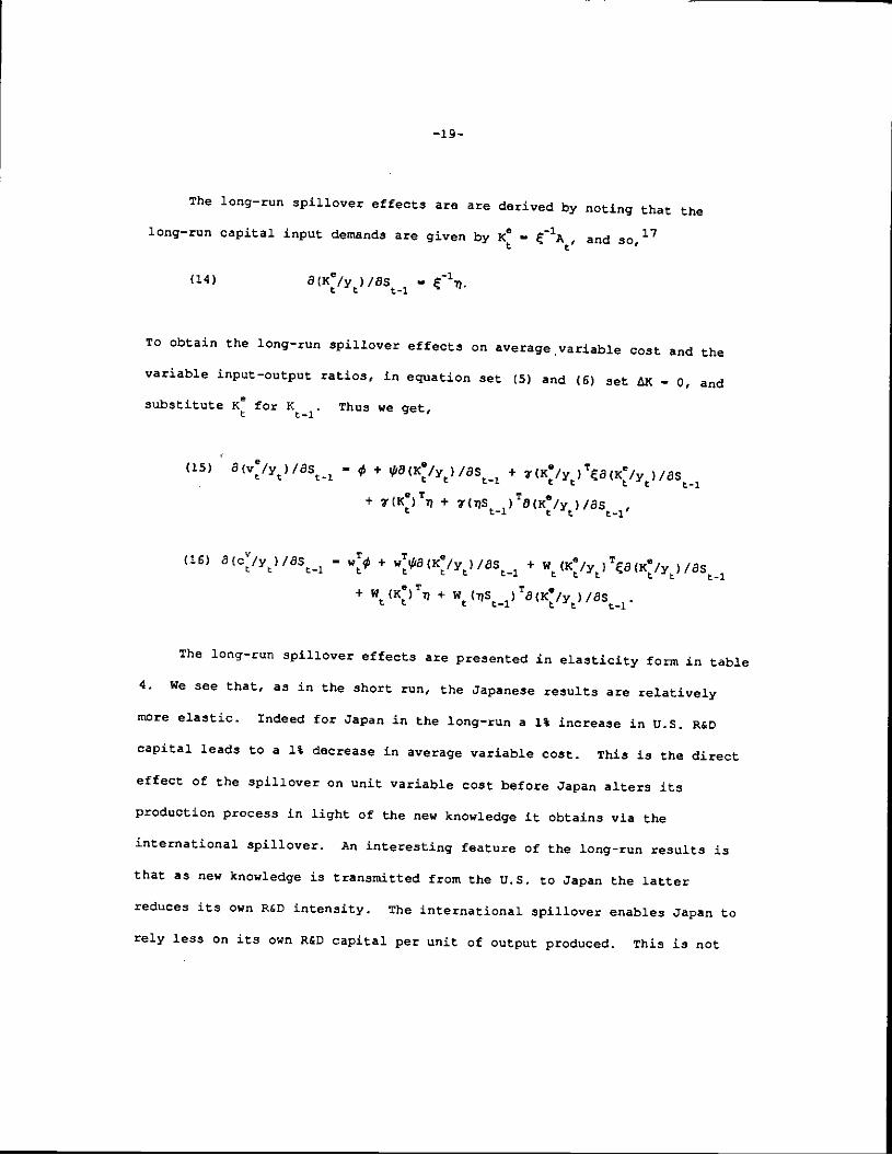
The long—run spillover effects are are derived by noting that the

long—run capital input demands are given by K: — and

(14) 3(x/y)/as —

To obtain the long—run spillover effects on average variable cost and the

variable input—output ratios, in equation set (5) and (6) set tic — 0, and

substitute f for K1. Thus we get,

(15) 8(Ve/Y)/3S — + c3(K/y)/as +

+ + v(s_l)To(x:,y),asl,

(16) 3(c/y)/3s — + w:a(K/Y),as +

+ + w(s)To(Ie,Y),aS

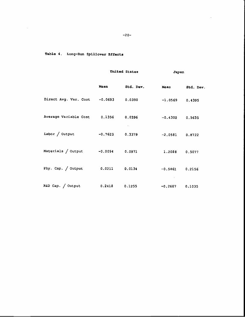
The long—run spillover effects are presented in elasticity form in table

4. We see that, as in the short run, the Japanese results are relatively

more elastic. Indeed for Japan in the long—run a 1% increase in U.S. R&D

capital leads to a 1% decrease in average variable cost. This is the direct

effect of the spillover on unit variable cost before Japan alters its

production process in light of the new knowledge it obtains via the

international spillover. An interesting feature of the long-run results is

that as new knowledge is transmitted from the U.S. to Japan the latter

reduces its own R&D intensity. The international spillover enables Japan to

rely less on its own R&D capital per unit of output produced. This is not

—20—

Table 4. Long-Run Spiflover Effects

United States Japan

Mean Std. Day. Mean Std. Day.

Direct Avg. Vat. Cost —0.0693 0.0390 —1.0569 0.4395

Average Variable Cost 0.1356 0.0396 —0.4300 0.5635

Labor / Output —0.7623 0.3379 —2.0581 0.8722

Materials / Output —0.0094 0.0971 1.2088 0.5077

Phy. Cap. / Output 0.0211 0.0134 —0.5461 0.2156

R&D Cap. / Output 0.2418 0.1255 —0.2607 0.1035

—21—

the case for the U.S., in the long—run, as in the short—run, R&D intensity

increases with the spillover fromJapan. The U.S. does not substitute its

own R&D capital per unit of output for theinternatjonaj spillover.

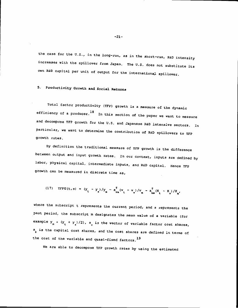
5. Productivity Growth and Social Returns

Total factor productivity (TFP) growth is a measure of the dynamic

efficiency of a producerj8 In this section of the paper we want to measureand decompcse TFP growth for the U.S. and

Japanese R&D intensive sectors. In

particular, we want to determine thecontribution of R&D SPillovers to TFP

growth rates.

By definition the traditional measure ofTFP growth is the difference

between output and input growth rates.In our context, inputs are defined by

labor, physical capital, intermediate inputs, and R&D capital. Hence TFP

growth can be measured in discrete time as,

(17) TFPG(t,s) (y — y )/y — s (v — v )/v — T(K — K )/Ks m Va t ' a km t s a

where the subscript t represents the current period, and s represents the

past period, the subscript in designates the mean value of a variable (for

example y (;+ y)/2), is the vector of variable factor cost shares,

is the capital cost shares, and the cost shares are defined in terms of

the cost of the variable and quasi—fixed factors.19

We are able to decompose TFP growth rates by using the estimated

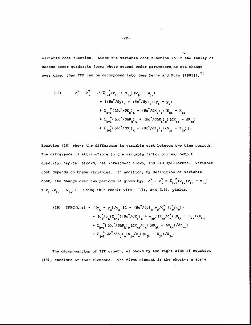
—22—

variable cost function. Since the variable cost function is in the family of

second order quadratic forms whose second order parameters do not change

over time, then TFP can be decomposed into (see Denny and Fuss (1983)1,20

(18) c — cV - .$t '(v + v ) (w — wt $ i—I. it is it is

+ (C8c/8Y) + (OcV/ay) ) Cy —

+ Eki((8c/ôKk)t + (8c"/BKk),) (K —Kk,)

+ S ( (Oc"/OAK ) + (ôcV/ÔM ) )(M — AKk—i k t k . kt cs

+ 5j((acv/OSj)t + (acV/aS)) (S1 — 5,)).

Equation (18) shows the difference in variable cost between two time periods.

The difference is attributable to the variable factor prices, output

quantity, capital stocks, net investment flows, and R&D spillovers. Variable

cost depends on these variables. In addition, by definition of variable

cost, the change over two periods is given by, c — — Z(w(v — v)+ v1(w1 — w1)). Using this result with (17), and (18), yields,

(19) TFPG(t,s) — ((y — y)/y) 11 — (8c"/ây) (yb") (c"Ic))

— (c"/c )S mUôc"/8K ) + w j (K Ic") (K — K )/Knm k—I.. kin km km. kt ks km

—

(oc"/OMk) (AKk/c) (Mkt— AK) /AKJ]

— S °(Oc"/8S ) (S Ic ) (S — S )/Sj—i jm jut m jt js jm

The decomposition of Tfl growth, as shown by the right side of equation

(19), consists of four elements. The first element is the short—run scale

—23—

effect, where (OcV/Oy) (y/Y) can be defined as the short—run cost

flexibility or the inverse of the short—run degree of returns to scale

(evaluated at the means of the variables). The second element relates to the

capital adjustment effects, which arise because the rental rate on each

capital input does not equal the cost reduction from this factor of

production. The third element consists of the adjustment cost effects

associated with both physical and R&D capital. The last element is the R&D

spillover effect.

The spillover effect can be further decomposed into two elements. These

two facets can be obtained from equation (13) where we observed that there is

both a direct and indirect effect of the spillover on variable cost. Noting

that Oc"/8S yO(c"/y)/ÔS, we can substitute the right side of equation (13)

into the last term on the right side of equation (19). The direct effect,

which is defined as the effect on variable cost when all input—output ratios

are held fixed, can be considered the traditional technological change effect

on TFP growth. Notice that although the spillover effect is exogenous to the

spillover receiver, it is not exogenous in the bilateral model of production,

since it is the R&D capital of the spillover source. The indirect spillover

effect on productivity growth represents the impact on factor intensities

from the new knowledge obtained from the foreign country.

Tfl growth and decomposition for the U.S. and Japanese R&D intensive

sectors are presented in table S. Japanese TFP growth generally exceeds the

rate obtained for the U.S. R&D intensive sector. Differences in TFP growth

are not that great until 1974. However, from the mid seventies until the mid

—24—

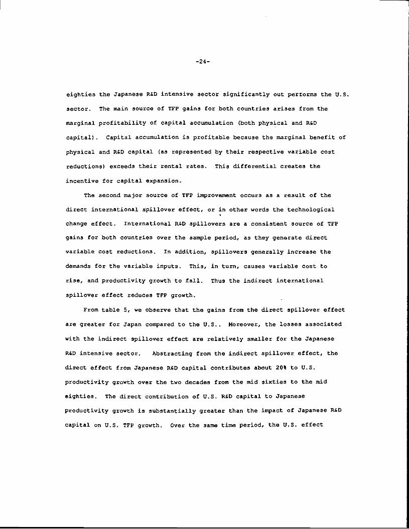
eighties the Japanese R&D intensive sector significantly out performs the U.S.

sector. The main source of Tfl' gains for both countries arises from the

marginal profitability of capital accumulation (both physical and R&D

capital) . Capital accumulation is profitable because the marginal benefit of

physical and R&D capital (as represented by their respective variable cost

reductions) exceeds their rental rates. This differential creates the

incentive for capital expansion.

The second major source of TFP improvement occurs as a result of the

direct international spillover effect, or in other words the technological

change effect. International R&D spillovers are a consistent source of TFP

gains for both countries over the sample period, as they generate direct

variable cost reductions. In addition, spillovers generally increase the

demands for the variable inputs. This, in turn, causes variable cost to

rise, and productivity growth to fall. Thus the indirect international

spillover effect reduces TFP growth.-

From table 5, we observe that the gains from the direct spillover effect

are greater for Japan compared to the U.S.. Moreover, the losses associated

with the indirect spillover effect are relatively smaller for the Japanese

R&D intensive sector. Abstracting from the indirect spillover effect, the

direct effect from Japanese R&D capital contributes about 20% to U.S.

productivity growth over the two decades from the mid sixties to the mid

eighties. The direct contribution of U.S. R&D capital to Japanese

productivity growth is substantially greater than the impact of Japanese R&D

capital on U.S. Tfl' growth. Over the same time period, the U.S. effect

—25—

Table 5. Decomposition of Average Annual TI'? Growth Rates

TF?G Scale Capital Adjust. Dirapil. Indspil.percent

United States

1963—1967 0.953 0.802 4.353 —3.861 0.175 —0.516

1968—1973 2.413 0.369 2.556 1.081 0.534 —2.127

1974—1979 —0.396 0.314 1.956 —0.180 0.405 —2.263

i.9BO—1985 —2.413 0.116 0.809 0.127 0.632 —4.097

1963—1985 0.104 0.219 2.334 —0.571 0.448 —2.326

Japan

1963—1967 1.749 —0.144 3.997 —1.685 1.136 —1.555

1968—1973 2.289 0.640 3.239 —1.830 1.125 —0.885

1974—1979 2.279 0.312 0.646 0.936 1.122 —0.737

1980—1985 1.394 0.000 1.118 —2.243 3.967 —1.448

1963—1985 1.935 0.217 2.174 —1.185 1.868 —1.139

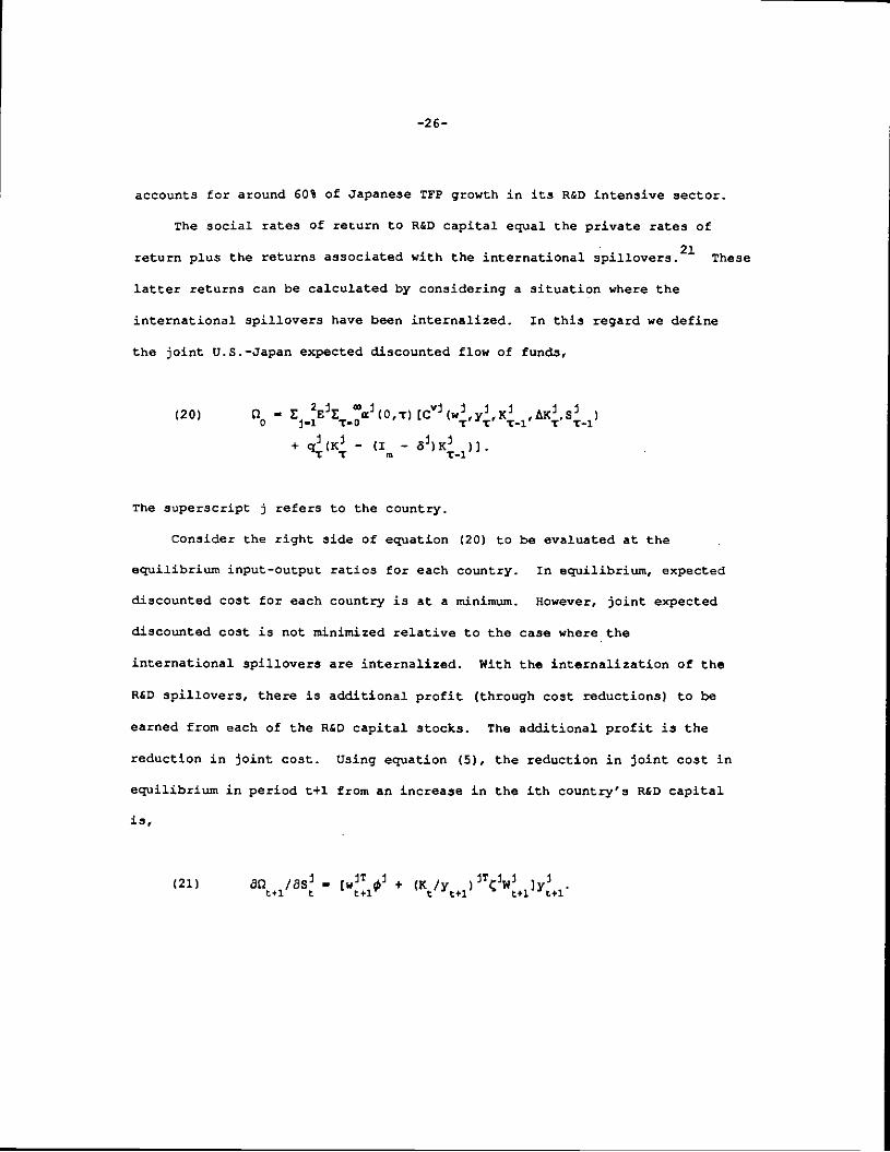
—26—

accounts for around 60% of Japanese TFP growth in its R&D intensive sector.

The social rates of return to R&D capital equal the private rates of

return plus the returns associated with the international spil1overs.2' These

latter returns can be calculated by considering a situation where the

international spillovers have been internalized. In this regard we define

the joint U.S.—Japan expected discounted flow of funds,

(20) — (C(w1,y4,K11AK,S1)+ cr1(K — (I — 5)1C H.

-V 'V 'V-i

The superscript j refers to the country.

Consider the right side of equation (20) to be evaluated at the -

equilibrium input—output ratios for each country. In equilibrium, expected

discounted cost for each country is at a minimum. However, joint expected

discounted cost is not minimized relative to the case where the

international spillovers are internalized, With the internalization of the

R&D spillovers, there is additional profit (through cost reductions) to be

earned from each of the R&D capital stocks. The additional profit is the

reduction in joint cost. Using equation (5), the reduction in joint cost in

equilibrium in period t+1 from an increase in the ith country's R&D capital

is'

(21) 8Q1/8S — (wØ +

—27—

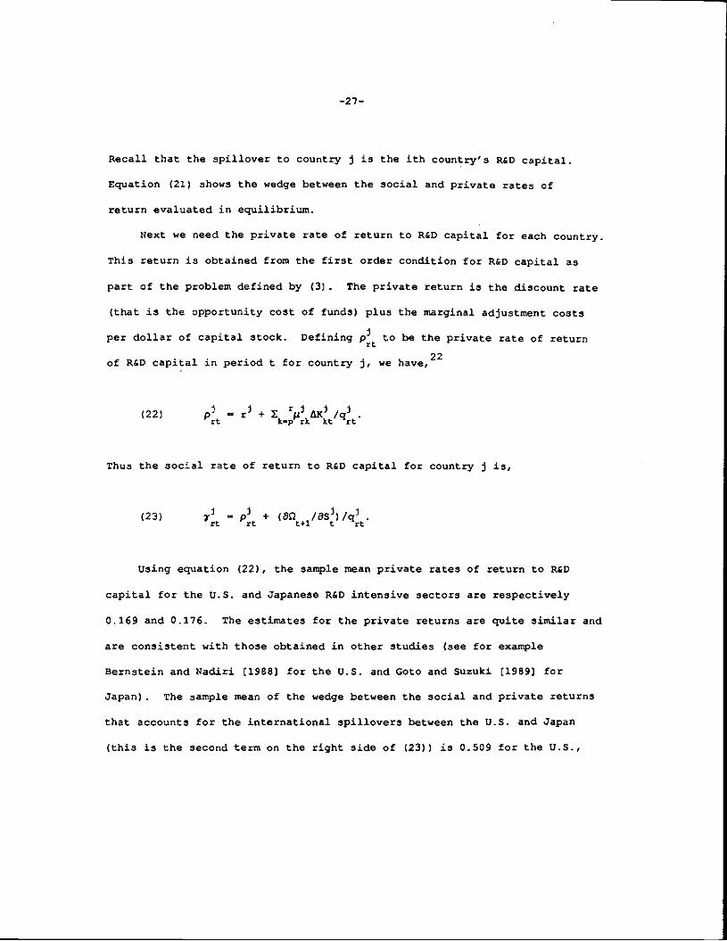
Recall that the spillover to country j is the ith Country's R&D capital.

Equation (21) shows the wedge between the social and private rates of

return evaluated in equilibrium.

Next we need the private rate of return to R&D capital for each country.

This return is obtained from the first order condition for R&D capital as

part of the problem defined by (3). The private return is the discount rate

(that is the opportunity cost of funds) plus the marginal adjustment costs

per dollar of capital stock. Defining p to be the private rate of returnof R&D capital in period t for country j, we have,22

(22) — r +

Thus the social rate of return to R&D capital for country j is,

(23) +

Using equation (22), the sample mean private rates of return to R&D

capital for the 13.5. and Japanese R&D intensive sectors are respectively

0.169 and 0.176. The estimates for the private returns are quite similar and

are consistent with those obtained in other studies (see for example

Bernstein and Nadiri (1968) for the U.S. and Goto and Suzuki [1969] for

Japan) . The sample mean of the wedge between the social and private returns

that accounts for the international apillovers between the U.S. and Japan

(this is the second term on the right aide of (23)) is 0.509 for the U.S.,

—28—

and 0.395 for Japan. Therefore the social rate of return for U.S. R&D

capital is 0.678 or more than 300% greater than the private rate of return.

For the Japanese R&D intensive sector the social rate of return is 0.571 or

about 225% greater than the private return.

The estimates of the social returns associated with the international

spillovers between the U.S. and Japan have not been previously calculated.

However, they are not out of line with the estimates associated with domestic

R&D spiflovers (see for example the survey by Nadiri (19931. It appears that

international spillovers are potentially as important as domestic spillovers.

6. Conclusion

The empirical results in this paper show that for the 13.5. and Japanese

R&D intensive sectors domestic production cost, traditional factor

intensities, and R&D capital intensity are affected by international R&D

spillovers between the two countries. These findings exist in both the short

and long—runs. However, there are important differences in the results

across runs and across countries. Short—run domestic R&D intensity is

complementary to the international spillover. In the U.S. a 1% increase in

the international spillover causes R&D intensity to rise by 0.02%, while for

Japan the effect is twice the U.S. elasticity. The complementarity persists

and becomes stronger for the U.S., in the long—run Japan substitutes U.S. R&D

capital for its own and thereby reduces its R&D intensity.

The most dramatic difference between the two countries has to do with

—29—

labor intensity. Japan reduces its labor intensity by 3.5% in response to a

1% increase in the international spillover from the U.S. . The corresponding

elasticity for the U.S. is only 0.01%. The Japanese R&D intensive sector

substantially increases its knowledge intensity as the international

spillover from the U.S. grows. In this situation we find that empirically

it is important to distinguish between short and long—run equilibrium

specifications, and to distinguish between the technologies in the U.S. and

Japan when investigating the effects of international spillovers.

International R&D spillovers directly contribute to productivity growthin both countries. International spillovers from the U.S. account for about

60% of Japanese productivity growth. The contribution front Japan to the U.S.

is smaller, but nevertheless not inconsequential, as the magnitude is 20%.

The existence of international spillovers imply that social rates of return

to R&D capital exceed private returns. We estimated that the private rates

of return to R&D capital are around 17% in both countries,, while the social

returns are three and a half to four times greater than the private return.

—30—

Footnotes

For a theoretical development of the international role of R&D capitalaccumulation see Ethier (1982], and Grossman and Helpman (1991).

2For simplicity, we do not introduce country specific notation. See

Diewert (1992) for the properties relating to production functions.

See Griliches [1979] for a discussion on the issues relating to R&Dspillovers in the production function. Bernstein and Nadiri (1999) haveapplied the production approach to the analysis of domestic intraindustry andinterindustry spillovers.

W is defined to be a Laspeyres price index of the variable factors ofproduction. Thus the y vector of coefficients consists of the variablefactor cost shares in the period of normalization, which is 1985.

Although there is the possibility of non—constant returns to scale, thedegree of returns to scale is assumed to be exogenous.

6We can also solve the model when expectations are based on autoregressive

processes, or when there is perfect foresight. In addition, if the capitalinputs are imediately productive then we just need to form expectations onreal output (y/W)

It should also be noted that the demand., for the variable factors are alsoaffected by the reparameterization of the solution to the capital inputs,since the parameter matrices M and appear in these demand equations.

The base period for the data in this paper is 1985. Thus we adjusted allU.S. price indexes to be one in 1985 and we adjusted the purchasing powerparities (PPP), obtained from Jorgenson and Kuroda (1990), to be indexed in1985. We also avoided double counting by subtracting the R&D expenditurecomponents from costs of labor, physical capital, and intermediate inputs.The R&D capital stock is developed by accumulating deflated R&D expenditures,assuming a depreciation rate of 10% (see Nadiri and Prucha (1993)) . Initialstocks were calculated by grossing up initial deflated expenditures by thedepreciation rate plus the growth rate of physical capital.

These industries also account for around 80% of manufacturing output andemployment in each country.

—31—

See Bernstein and Nadir! ttgeej for results on U.S. interindustryspillovers, and Goto and Suzuki (1989] for results on Japanese industries.

In the estimation of equation sets (6), and (9), we can impose theconditions that the variable cost function must be concave in the variablefactor prices and convex in the capital inputs and net investment. Theseconditions result in the following parameter restrictions, — — DD, -EE and ji — GG , where D,E and G are lower triangular matrices. We do notimpose these conditions because the estimates turn out to satisfy them. Inorder to identify the parameters we impose the restriction that i — 0

I'where i is the unity vector.

12The definition of returns to scale is inclusive of the R&D capital input

and adjustment costs in both physical and R&D capital inputs, There are noprevious estimates of returns to scale in these sectors, as a whole, althoughNadir! and Prucha [1990] found slightly increasing returns to scale in theU.S. and Japanese electrical products industries.

13The dummy variable is associated with the parameter matrix 0, because the

test regarding the flexible accelerator can only be conducted in a short—runequilibrium.

14Under constant returns to scale the model was estimated in ratio form. In

other words the endogenous variables are input—output ratios.

15The correlation coefficients are between observed and predicted endogenousvariables, where the predicted values are computed from the reduced form

estimated equations. In addition, we see from table 1 that without imposingthe curvature conditions that the variable cost function is concave in thevariable factor prices as fi11<0, the function is convex in the capital inputsas b <0, i — p,r, and b b — b2 >0 (recall that the B matrix is negativelyii pprr prrelated to the matrix from equations (7) and C9)), and the function is

convex in net investments as $L>0, i — p,r, and MppMrr —

16The directional changes found for international spillovers are similar to

those obtained from domestic spillover studies in the U.S. and Japan (seeBernstein and Nadiri (1988] and Gob and Suzuki (1989]).

17See equation (7), and the discussion that follows.

—32—

18 See Denny and Fuss t19831, and Diewert (1989] for discus3ions of thedifferent measures and interpretations of productivity growth.

19 All current period capital stocks refer to the beginning of periodquantities which are lagged one period.

20 A unit variable cost function was estimated. However, this does not posea problem for the Tfl' decomposition, since ac"/az — ya(cV/y)/Oz + 8, —

c"/y if z — y, and 0 otherwise.

21 The private rates of return relate to the R&D intensive sector in each

country. In addition, any intrasectoral spillovers have been internalized.Since we are focusing on international spillovers, domestic spilloversbetween the R&D intensive sector and other sectors of the economy of a

country are assumed to be inconsequential. This appears to be reasonablesince about 90% of R&D investment in both the U.S. and Japanese economies areperformed within the R&D intensive sector.

22The rate of return for R&D capital is found from the Euler equation by

equating the expected marginal benefit to the expected marginal cost. Theformer is the expected future cost reductions (including adjustment costsavings) net of depreciation per dollar of capital stock. Theexpected marginal coat is the discount rate plus marginal adjustment costsper dollar of capital stock. The rates of return on R&D capital are definedas before tax returns.

—33—

Referencea

Berndt, E., and H. Fuss: Productivity measurement with adjustmentsfor

variations in capacity utilization and other forms of temporaryequilibrium, Journal of Econometrics, 33,7—29, 1986.

Bernstein,J.I., and P. Mohnen: Price—cost margins, exports andproductivitygrowth: with an application to Canadian industries, Canadian Journal of

Economics, 24, 638—659, 1991. —Bernstein, LI. and 14.1. Nad.iri: Research and development and

intraindustryspillovers: an empirical application of dynamic duality, Review ofEconomic Studies 56, 249—269, 1989. —

Bernstein, J.I. and 14.1. Nadiri: Interindustry R&D spillovers, rates ofreturn and production in high—tech industries, American EconomicReviewr, Papers and Proceedings 78, 429—434, 1988.

Cohen, W., and R. Levin: Empirical studies of innovation and marketstructure, in R. Schmalensee and R. Willig, eds., Handbook of IndustrialOrganization 2, Elsevier Science Publishers, Amsterdam, The

Netherlands,1989.

Cohen, W., and D. Levinthal: Innovation and learning: the two faces of R&D-implications for the analysis of R&D investment, Economic Journal, 99,569—596, 1989.

Denny, M., Bernstein, J.I., Fuss, H., Nakamura, S. and L. Waverman:Productivity in manufacturing industries, Canada, Japan and the UnitedStates 1953—1986, Was the 'productivity slowdown' reversed?, CanadianJournal of Economics 25, 584—592, 1992.

Denny, H., and M. Fuss: The use of discrete variables in superlative index

number comparisons, International Economic Review, 24, 419—421, 1983.

Diewert, W.E.: Fisher ideal output, input and productivity indexes revisited,University of British Columbia, Dept. of Economics, Discussion Paper89—07, 1989.

Diewert, W.E.: Duality approaches to microeconomic theory, in K. Arrow andM. Intrilligator, eds., Handbook of Mathematical Economics 2, ElsevierScience Publishers, Amsterdam, The Netherlands, 1982.

Diewert, W.E. and T.J. Wales: Flexible functional forms and global curvatureconditions, Econometrica 55, 43—68, 1987.

Epstein, L. and A. Yatchew: The empirical determination of technology andexpectations: a simplified procedure, Journal of Econometrics 27,235—258, 1985.

—34—

Ethier, W: oecreasing costs in international trade and Frank Graham'sargument for protection, Econometrics, 50, 1243—1268, 1982.

Goto, A., and K. Suzuki: R&D capital, rate of return on R&D investment and

spillover of R&D in Japanese manufacturing industries, The Review ofEcononti-cs and Statistics, 71, 555—564, 1999.

Griliches, Zvi: Issues in assessing the contributions of research anddevelopment to productivity growth, Bell Journal of Economics, 10,

92—116, 1979.

Griliches, Zvi: Productivity puzzles and R&D: Another nonexplanation,Journal of Economic Perspectives, 2, 9—21, 1988.

Grossman G. M., and E. Helpman: Innovation and Growth in the Global Economy,

MIT Press, Cambridge, Massachusetts, 1991.

Jorgenson, D.W. and M. Kuroda: Productivity and internationalcompetitiveness in Japan and the United States 1960—1985, in C.Hulten, ed., Productivity Growth in Japan and the United States,

University of Chicago Press, Chicago, 1990.

Jorgenson, D.W., H. Sakuramoto, K. Yoshioka, and H. Kuroda: Bilateral modelsof production for Japanese and U.S. industries, in C. Rulten, ed.,Productivity Growth in Japan and the. United States, University of

Chicago Press, Chicago, 1990.

Jorgenson, D.W. and H. Nishntu. . U.S. and Japanese economic growth1952—1974, an international comparison, Economic Journal 88, 707—726,1978.

Mohnen, P.A., 14.1. Nadiri and I.R. Prucha: R&D production structure, andrate of return in the U.S., Japanese and German manufacturing sectors: anon—separable dynamic factor demand model, European Economic Review 30,

749—771, 1986.

Morrison, C: Unraveling the productivity growth slowdown in the United

States, Canada and Japan: the effects of subequilibriuiii, scaleeconomies and markups, The Review of Economics and Statistics, 74,

381—393, 1992.

Morrison, C. and E. Berndt: Short—run labor productivity in a dynamic model,Journal of Econometrics 15, 339—365, 1981.

Nadiri, WI: Innovation and technological spillovers, NBER Working Paper no.4423, 1993.

Nadiri, 14.1., and I. Prucha: Estimation of the depreciation rate of physicaland R&D capital in the U.S. total manufacturing sector, NBER WorkingPaper no. 4591, 1993.

—35—

Nadiri, 11.1., and I.R. Prucha: Comparison and analysis ofproductivity growthand R&D investment in the electrical machinery industries of the United

States and Japan, in C.R. Hulten ed., Productivity Growth in Japan andthe United States, University of Chcago Press, Chicago, 1990.