NBER WORKING PAPER SERIES

GOOD VERSUS BAD DEFLATION:LESSONS FROM THE GOLD STANDARD ERA

Michael D. BordoJohn Landon Lane

Angela Redish

Working Paper 10329http://www.nber.org/papers/w10329

NATIONAL BUREAU OF ECONOMIC RESEARCH1050 Massachusetts Avenue

Cambridge, MA 02138February 2004

This paper was prepared for the Federal Reserve Bank of Cleveland's ‘Conference on Low InflationEconomies’, November 20-21 2003. For helpful comments we thank: Tam Bayoumi, Jon Faust, DaleHenderson, Ulrich Kohli, Andy Levin, Marc Wiedenmeir, and our discussants: Larry Christiano and FrancoisVelde. For able research assistance we thank Sonal Dhingra. The views expressed herein are those of theauthors and not necessarily those of the National Bureau of Economic Research.

©2004 by Michael D. Bordo, John Landon Lane, and Angela Redish. All rights reserved. Short sections oftext, not to exceed two paragraphs, may be quoted without explicit permission provided that full credit,including © notice, is given to the source.

Good versus Bad Deflation: Lessons from the Gold Standard EraMichael D. Bordo, John Landon Lane, and Angela RedishNBER Working Paper No. 10329February 2004JEL No. E3, N20

ABSTRACT

Deflation has had a bad rap, largely based on the experience of the 1930's when deflation was

synonymous with depression. Recent experience with declining prices in Japan and China together

with the concern over deflation in Europe and the United States has led to renewed attention to the

topic of deflation. In this paper we focus our attention on the deflation experience of the United

States, the United Kingdom, and Germany in the late nineteenth century during a period

characterized by low deflation, rapid productivity growth, positive output growth, and where many

nations had a credible nominal anchor based on gold: circumstances which have resonance with the

world of today. We identify aggregate supply, aggregate demand, and money supply shocks using

a structural panel vector autoregression. We then use historical decompositions to investigate the

impact that these structural shocks had on output and prices. Our findings are that the deflation of

the late nineteenth century reflected both positive aggregate supply shocks and negative money

supply shocks. However, the negative money supply shocks had little effect on output. This we posit

is because the aggregate supply curve was very steep in the short run during this period. This

contrasts greatly with the deflation experience during the Great Depression. Thus our empirical

evidence suggests that deflation in the nineteenth century was primarily good.

Michael D. BordoDepartment of EconomicsRutgers UniversityNew Brunswick, NJ 08901and NBERbordo@econ.rutgers.edu

John S. Landon-LaneDepartment of EconomicsRutgers UniversityNew Brunswick, NJ 08901lane@econ.rutgers.edu

Angela RedishDepartment of EconomicsUniversity of British ColumbiaVancouver, B.C.Canada, V6T 1Z1anji@econ.ubc.ca

1

I. Introduction

Recent concerns by the FOMC at its meeting in May 2003 that the "balance of

risks in the US had shifted in favor of deflation", similar concerns raised by an IMF

Report on Deflation (2003) over the risk of deflation in Europe, especially Germany and

Switzerland, and the experience of declining price levels in China and Japan has sparked

new interest in the subject of deflation. In this paper we examine the issue from an

historical perspective. We focus on the experience of deflation in the late nineteenth

century when most of the countries of the world adhered to the classical gold standard.

The period 1880-1914 was characterized by two decades of secular deflation followed by

two decades of secular inflation.

The price level experience of the pre-1914 period has considerable resonance for

recent concerns over the possibility of deflation’s re-emergence. Four elements of the

earlier experience are relevant for today’s environment: deflation was relatively low (1-

3% in most countries); productivity advance was rapid; the real economy was growing;

and the price level was anchored by a credible nominal anchor – adherence to gold

convertibility.

Deflation has had a ‘bad rap’. Possibly as a consequence of the combination of

deflation and depression in the 1930s, deflation is associated with (for some, connotes)

depression. In contrast, a basic tenet of monetary theory – the Friedman rule – suggests

that deflation (albeit perfectly anticipated) is an outcome of optimal monetary policy. On

the face of it, the evidence from the late 19th century was mixed: on the one hand, the

mild deflation in the period 1870 - 1896 was accompanied by positive growth in many

countries, however, growth accelerated during the period of inflation after 1896.

We distinguish between good and bad deflations. In the former case, falling prices

may be caused by aggregate supply (possibly driven by technology advances) increasing

more rapidly than aggregate demand. In the latter case, declines in aggregate demand

outpace any expansion in aggregate supply. For example, negative money shocks that are

2

non-neutral over a significant period would generate a ‘bad’ deflation. This was the

experience in the Great Depression (1929-33), the recession of 1919-21, and may be the

case in Japan today.1 There is also a third possibility – the Classical case where deflation

– for example caused by negative money shocks - is neutral, as when monetary neutrality

holds.2

We focus on the price level and growth experience of the United States, the U.K.

and Germany from 1880-1913. All three countries adhered to the international gold

standard, under which the world price level was determined by the demand and supply of

monetary gold, and each member followed the rule of maintaining convertibility of its

national currency into a fixed weight of gold. This meant that the domestic price level

was largely determined by international (exogenous) forces.

We proceed by identifying separate ‘supply’ shocks, money supply shocks and

‘non-monetary’ demand shocks using a Blanchard-Quah methodology. We identify the

shocks by imposing long run restrictions on the impact of the shocks on output and

prices, and then do a historical decomposition to examine the impact of each shock on

output and the price level.3 We present three sets of empirical results: firstly, results for

each country from estimating a panel over the period 1880-1913, then results from

estimating a panel over only the deflationary period, 1880-96, and finally results from the

entire period in a model in which gold supply shocks are included as an exogenous

variable. Contrasting the first two series of results enables us to discuss the symmetry

between the deflationary and inflationary period, while in the third set we separate money

supply shocks coming from gold shocks from those coming from intermediation shocks.

1 The traditional explanation for this non-neutrality is nominal rigidities and more recently balance sheet effects are also ascribed an important role (Bernanke, 1983). 2 Many people take issue with the term “good” deflation on the view that any departures from price stability are problematic. An alternative set of terms that we could use are “benign” versus “malignant” deflation or “the good, the bad and the ugly” as used by Borio and Filardo (2003). These terms connote: productivity driven deflation as used by us; low deflation and stagnation as has been the case in Japan; and the interwar experience. 3 A similar methodology is followed in Bordo and Redish (2004). The results of the historical decompositions for the money stock, as well as the results from forecast error variance decompositions, are not presented in this paper for space reasons, but are available from the authors on request. The results are consistent with those reported in this text.

3

The paper begins by briefly describing the data and historical environment. We

then discuss the empirical methodology to be used. Our empirical analysis is presented in

the next three sections, and the final section discusses the results and their implications

and limitations.

Focussing on our interest in the deflationary episode, our results in a nutshell

suggest that the deflation was generated by monetary factors, but that these monetary

factors do not explain much of the behaviour of output. Output was determined by non-

monetary factors and the deflation was essentially good or neutral.

II. The context

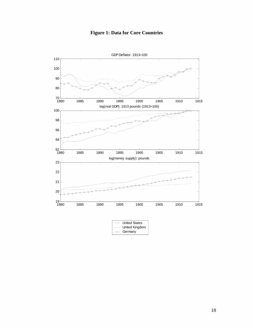
Figure 1 illustrates the behaviour of the money stock, prices (GDP deflators) and

real incomes in the three countries over the period 1880 - 1913. We use broad money

(M2) as our measure of money stock, real GDP as our measure of real income and the

GDP deflator as our measure of prices.4 While there are differences in the patterns there

are a few common trends: price levels declined – more in the U.S. than elsewhere - over

the period 1880 to the mid 1890s, and subsequently rose. The money stock rose secularly,

the most pronounced rise occurring in Germany, and in the U.S. the growth rate increased

after 1896. Income levels rose with a slight acceleration in the US and UK after the

1890s, but German output growth decelerated (very slightly) from its very rapid post-

1870s rate after the mid-1890s.

The period 1880-1913, encompassed myriad economic events. Technological

changes occurred rapidly, and earlier changes were implemented at the production level.

German and US growth outpaced that of England. Early historians had described the

period before 1896 as a ‘great depression’ but more recent historiography has recast the

period as one of deflation without depression (Craig and Fisher, 2000). Although there

were very severe recessions, particularly in the early 1890s, secularly incomes rose. 4 Data are available from the authors on request. Sources: US – Balke and Gordon (1986); UK – Mitchell (1998); Germany – Prices: Sommariva and Tullio (1987); GDP: Mitchell (1998); Money: Deutsche Bundesbank (1976). Real output is denominated in 1913 pounds sterling while nominal money supply is denominated in current pounds sterling. The GDP deflators are used as the price series and these are based in 1913.

4

Particularly noteworthy is the transmission of business cycles across economies, with all

three of our economies experiencing common cycles.5

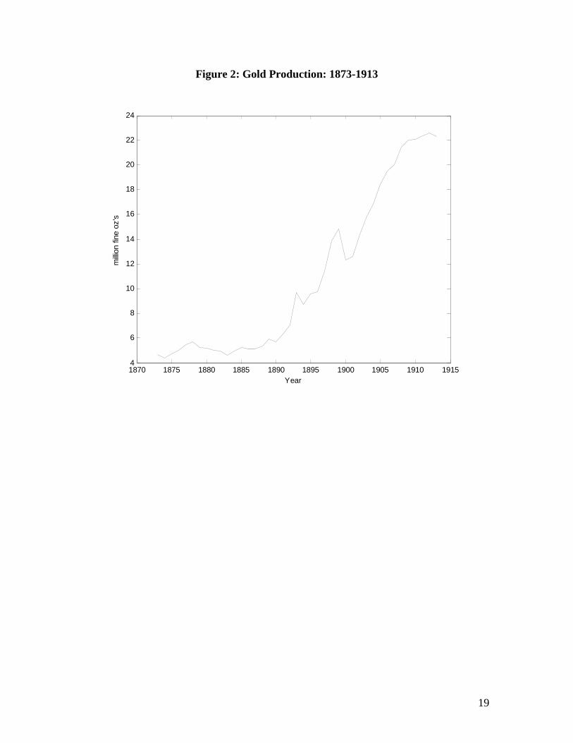
At the monetary level there were also secular trends and cyclical fluctuations. The

gold standard tied the quantity of money to the stock of gold. Figure 2 shows that world

gold production was constant and relatively low from 1870 to 1890 while after the early

1890s it grew. The growth reflected gold discoveries in South Africa as well as Australia

and North America.

III. Methodology

Our empirical analysis is grounded by a model of money supply under the gold

standard. The appropriate modeling strategy depends on the time horizon of interest,

whether one is interested in the very long run, the long run or business cycle frequency.

The ‘very long run’ we consider to be a period long enough for the quantity of gold

mined to respond endogenously to macroeconomic variables.6 Given the short span of

data available for our empirical analysis, we do not attempt to capture effects over this

period, and restrict ourselves to long run and business cycle frequencies.

The long run is defined here as a period over which purchasing power parity

holds, and we model a world comprising several gold standard economies linked together

by trade in gold, goods and capital. We assume that in each economy the quantity of

money is a stable function of the country’s stock of monetary gold, but the function is

allowed to vary across countries reflecting, for example, the existence or not of a central

bank, required reserve ratios, the degree of monetization and the nature of the banking

system. The world price level is determined by the world demand for money (based on

the determinants of velocity and aggregate income) and the supply of money (the supply

being determined by stocks of gold and the nature of intermediation). Individual

economies take the world price level as exogenous. For each country we identify three 5 See IMF (2002) and Bergman, Bordo and Jonung (1998). 6 For example, models in Bordo and Ellson (1985) and Dowd and Chappell (1997) allow the quantity of gold mined to respond endogenously to the price level, through investment in refining technologies and exploration. See also, Barro (1979) and Rockoff (1984). Rockoff argues that the increased gold production of the late 19th century was a response to the incentive of the high real price of gold (i.e. low price level).

5

shocks that drive the joint behaviour of prices, output and the money stock: a money

supply shock, a technology shock, and a non-monetary demand shock, where the

definition of each shock is implicit in the identifying assumptions described below.

We model output, prices and money supply using the following tri-variate VAR

in differences:

(1) ∑=

− +∆+=∆p

jtjtjtt yBDy

1

εα ,

where ( )tttt MGDPpricey ,,= and Dt is a matrix of deterministic variables that includes

a constant and possibly a time trend. The data are tested for the presence of a unit root

and are differenced to make them stationary.

Underlying the reduced form specification, (1), is a set of structural innovations,

ut, that are orthogonal to each other and are related to the reduced form innovations in (1)

by

(2) tt Cu=ε .

Our aim is to identify orthogonal shocks, ut, that can be interpreted as an

aggregate supply shock, a nominal money supply shock and a non-monetary aggregate

demand shock. To this end, we identify C by imposing long-run restrictions on the

structural impulse response functions implied by (1). These long-run restrictions are

imposed using the method described in Blanchard and Quah (1989).

In order to exactly identify C for each country, we need to impose at least three

independent long-run restrictions on the impulse response functions from (1). Our

preferred identification is as follows: An aggregate demand shock is assumed to have

zero long-run impact on output and prices. That is, the demand shock has no permanent

impact on prices or output. We also assume that the aggregate supply shock, in the

context of the gold standard, has no permanent impact on prices. That is, the long-run

impact of an aggregate supply shock on price is zero.

6

This identifying restriction follows from the fact that the countries in our sample

were all strictly adhering to the gold standard during the sample period. An aggregate

supply shock would be expected to initially lower the price level and increase real output.

The decline in the price level would lead in turn to a gold inflow via the current account,

hence raising the money supply and price level. Thus, gold flows will have the effect of

causing price levels, in the absence of further shocks, to return to their original levels.

These three long-run restrictions are enough to exactly identify C and hence

identify the structural shocks, ut. We thus impose no restrictions on the impact of the

third shock. This is the only long run influence on the price level and can be interpreted

as a world price level shock or, in the context of our model, as a money supply shock.

The aggregate demand shocks are presumably an aggregate of money demand shocks and

temporary spending shocks, which cannot be disentangled. The effect of such an

aggregate on prices and output in the short run would depend on its component mix, and

we essentially treat this as a reduced form construct.

A summary of our preferred identifying restrictions is:

1. An aggregate supply shock has no long-run impact on prices.

2. An aggregate demand shock (combining the impact of velocity and spending

shocks) has no long-run impact on either prices or output.

3. The long run (and short run) impact of a nominal money supply shock on money,

output and prices is unrestricted.

The long-run impact of shocks to ut, the structural innovation vector, is

(3) CAILR 1))1(( −−= ,

where pp LALAILA −−−= K1)( and ∑−= =

pj jAIA 1)1( . Assuming that the structural

innovation vector is ordered as )shockdemand,shocksupply ,shockmoney( ′= ttttu then

the long-run impact matrix is

7

(4)

=

333231

2221

11

0

00

LRLRLR

LRLR

LR

LR .

In addition to our preferred identification there are other possible long-run

restrictions that could have been imposed. The most likely additional restriction is money

neutrality, which would imply that the long-run impact of a money shock on output is

zero. The addition of this long-run restriction leads to the long-run impact matrix

(5)

=

333231

22

11

00

00

LRLRLR

LR

LR

LR .

Clearly this leads to an over-identified system. Following the method described in

Amisano and Giannini (1997), the over-identifying restrictions imposed in (5) can be

tested. If this extra long-run identification cannot be rejected it will be imposed.

However, we prefer not to impose money neutrality but rather allow the data to tell us if

money neutrality holds during this sample. Only then do we impose this additional long-

run restriction.

Another possible combination of the four long-run restrictions given in (4) and (5)

would be

(6)

=

333231

22

1211

00

0

LRLRLR

LR

LRLR

LR .

In this specification money neutrality would be imposed while the impact of the supply

shock would be unconstrained. The set of constraints given in (6) exactly identify the

structural shocks. If (5) is rejected we are left with a decision on whether to use (4) or (6),

and opt for (4) on the basis of the historical context.

Given the small sample size inherent in the data there are efficiency gains from

pooling the data and estimating a panel VAR (PVAR) given by

8

(7) ∑=

− Σ+∆+=∆p

jiititjitijitit NyBDy

1

),0(~εεα .

The maintained assumption in this exercise is that the slope coefficient matrices,

Bij, are common across the countries in the panel. Different growth rates between

countries and periods are allowed by permitting the constant terms in each VAR to be

different. Also, the variance-covariance matrix of the innovations for each country

specific VAR, i∑ , is allowed to differ across countries. This assumption allows for cross-

sectional heteroscedasticity in the data. One implication of permitting cross-sectional

heteroscedasticity is that individual countries are not constrained to have the same

responses to structural shocks. All that is being assumed is that all countries have the

same slope coefficient matrices in the reduced form VAR. Also, the values of the slope

coefficients do not change throughout the sample. These two assumptions are tested and

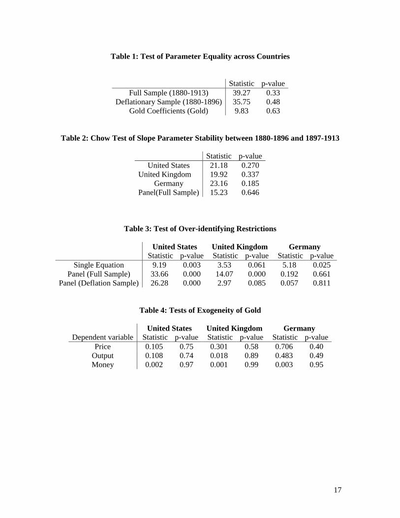
the results of these tests are reported in Table 1 and Table 2.

The PVAR in (7) is estimated using the standard seemingly unrelated regression

estimator (SURE) with cross-equation restrictions imposed as defined above. This allows

us to exploit the panel structure and any contemporaneous correlation in shocks between

countries to improve the efficiency of our estimates. After estimating our PVAR we then

estimate Ci for each country using the scoring algorithm defined in Amisano and

Giannini (1997) and use these estimates to calculate structural impulse response functions

for each country. Once we have Ci we are also able to construct the structural shocks

implied by (2).

The structural impulse response functions isolate the impact of each of our

identified shocks on each variable. Since we impose no restrictions on the impact effects

of the shocks, we can use consistency between the theoretical predictions for the impact

effects and the estimated impulse response functions to make the case that our economic

interpretation of the estimated shock is valid. Having made that case, the historical

decompositions allow us to do the counterfactual analysis that is inherent in our

questions: How would output and prices have evolved if there had been no monetary

9

shocks? What were the relative contributions of money and real shocks to the late 19th

century deflation? These results are reported in the next Sections.

IV. Results – Full Sample

Prior to estimation we analyzed the time series properties of the data and

concluded that all the series were I(1) and we therefore estimated the model in first

differences. That is, we estimated (7). Information criteria tests suggested that a model

with two lags fit the data well (that is p=2), and we included a trend break in all series in

1896. Given that the series are all non-stationary and that we estimated (7), the break in

trend is handled by putting a dummy variable that takes the value of 0 before 1897 and

takes the value of 1 from 1897 until 1913. Clearly using two lags in (7) would have

severely affected the degrees of freedom of the estimator for the individual estimation.

Table 1 reports tests of slope parameter equality across the countries in the sample. That

is, Table 1 reports Wald test results for the test given in (8):

(8)

.,:

.

,:0

jsomeforandkisomeforBBH

vs

jeachforkiBBH

kjijA

kjij

≠

∀=

This test was performed using data from the whole sample (1880-1913) and using

data for the deflationary sample (1880-1896). In both cases the null hypothesis could not

be rejected so that our assumption of similar short-run dynamics across the countries in

our panel is not rejected by the data. Given that there appears to be a trend break in 1896

a test was performed to see if there was also a structural break in the short-run dynamics

of the VAR. That is, we tested to see if the estimates of Bij were significantly different for

the two different periods. Results from these tests are reported in Table 2. For each

country individually and for the panel estimate there is no evidence of a structural break

in the short-run dynamics of the system. Therefore, we account for the break in trend

with intercept adjustments only.

Structural impulse response functions were estimated using identifications (4) and

(5). The over-identifying restrictions in (5) were tested and these results can be found in

10

Table 3. Estimating (1) using data from each country individually we see that the over-

identifying restrictions are rejected for each country. When we estimate (7) using the

panel estimator we see that neutrality is rejected for the US and the UK but not for

Germany. Therefore we do not impose neutrality and so use identification (4) to compute

the structural impulse response functions.

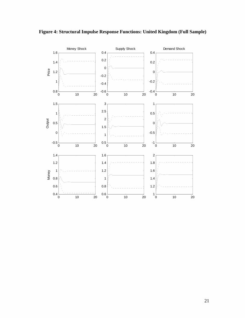
Structural impulse response functions showing the impact of a 1% shock are

reported in Figures 3 through 5. Standard error bands show 90% approximate asymptotic

confidence intervals calculated using the method described in Amisano and Giannini

(1997).7 We observe for all countries that the money supply shock has a large positive

impact on output in the short run, and a much smaller (zero for Germany) long run

positive impact. In the US, prices and the money stock rise proportionately in response to

the money shock, though in the other countries the price effect is larger. In each case the

supply shock is observed to cause a significant temporary decline in prices (recall that the

long run impact is imposed to be zero). In the US, the long run income elasticity of

money is roughly unitary (that is, the money stock increases proportionately with

increases in income) while in Germany and the UK it is somewhat less that unitary.

Consistently with the interpretation as a demand shock, the direction of the impact of the

third shock is the same for prices and output. In each case the shock has a negative short

run impact on prices and output, and a positive impact on money stocks, which is

consistent with an interpretation that velocity shocks dominated the demand influences.

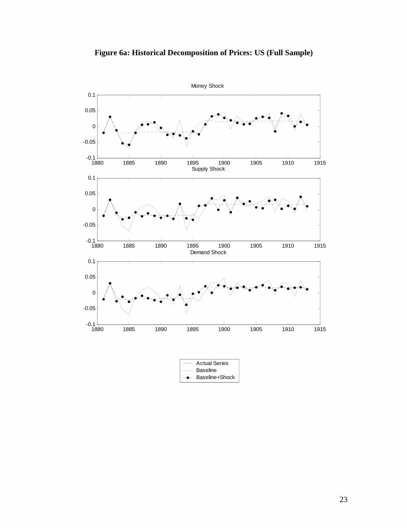
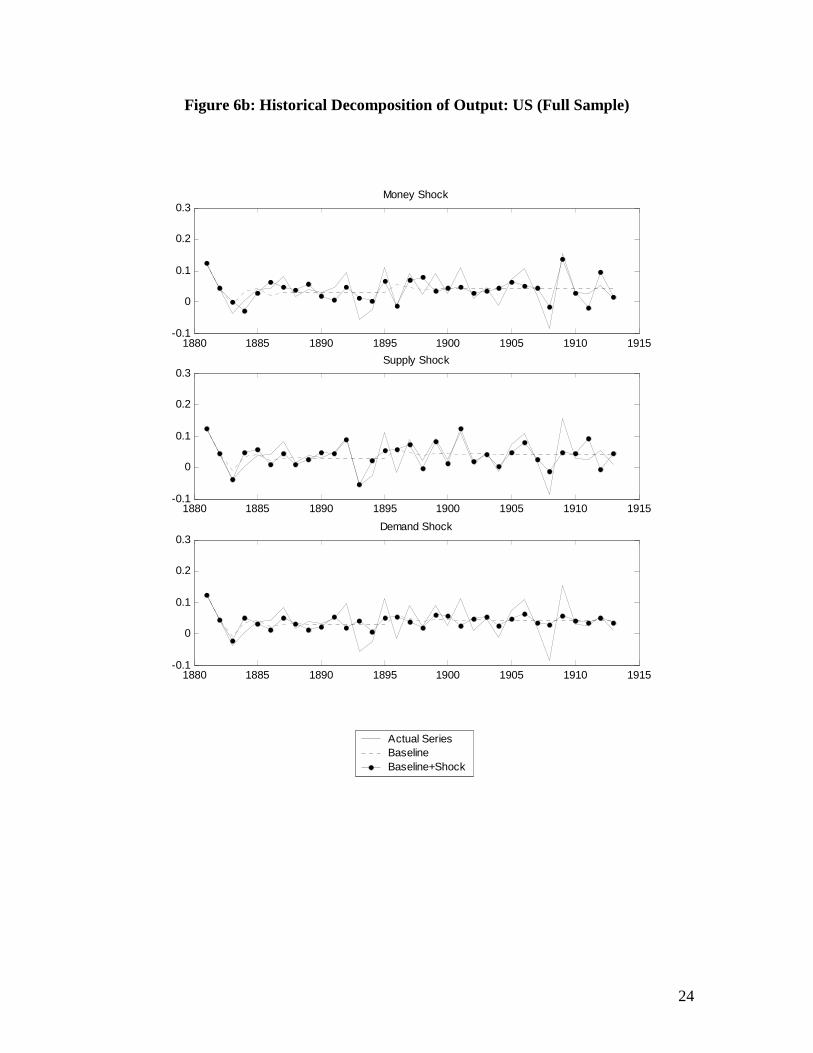
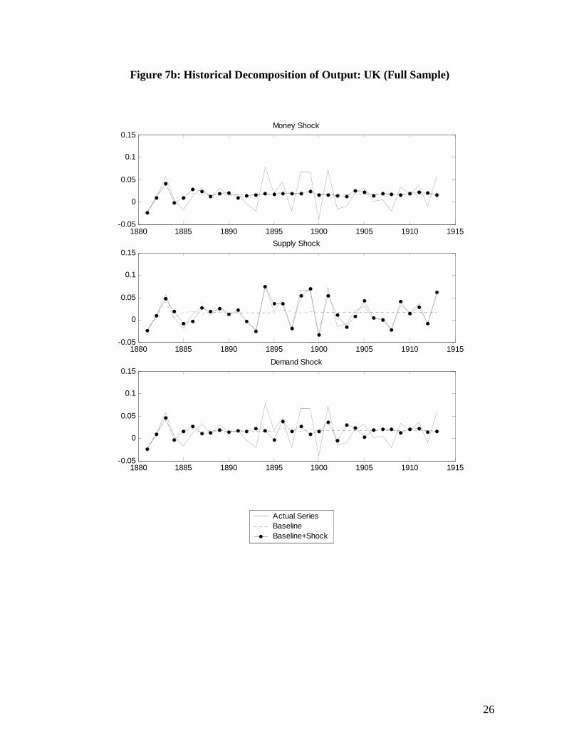
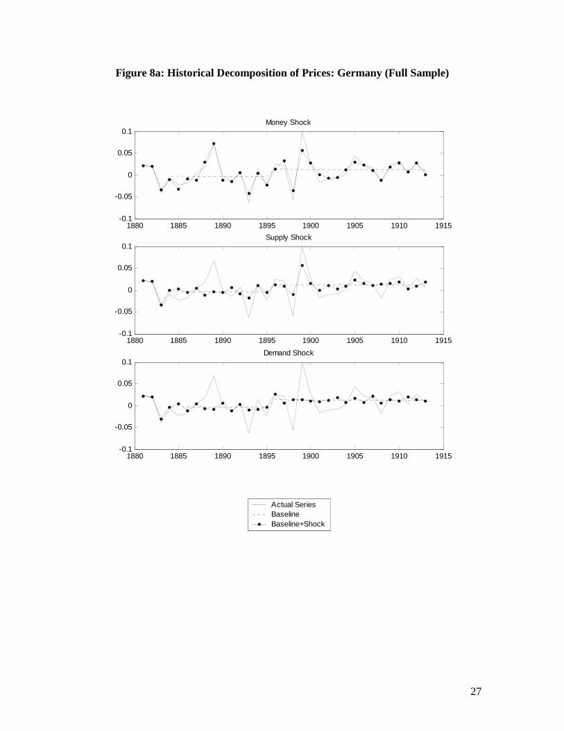
Historical decompositions for each shock are reported in Figures 6 through 8.

The three panels each contain plots of three series: the actual path of the variable, a

baseline – which incorporates trends and shocks before the estimated period but none of

the shocks during the estimated period; and a line showing the baseline plus the effect of

one of the structural shocks. If the third line lies essentially on top of the baseline, then

the isolated shock had no effect on the variable, while if the third line lies on top of the

actual line, it shows that the isolated shock accounts for the behaviour of the variable.

7 In fact probably less than 90% given our small sample size.

11

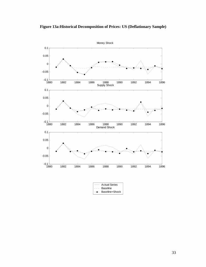
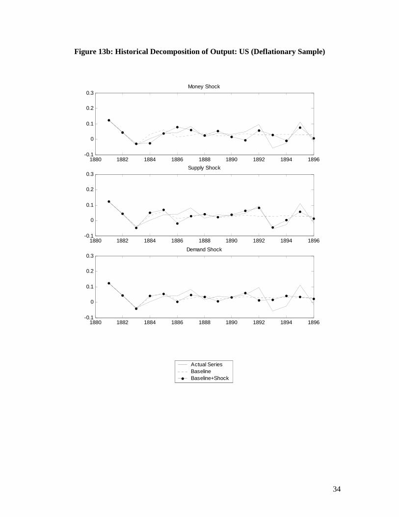
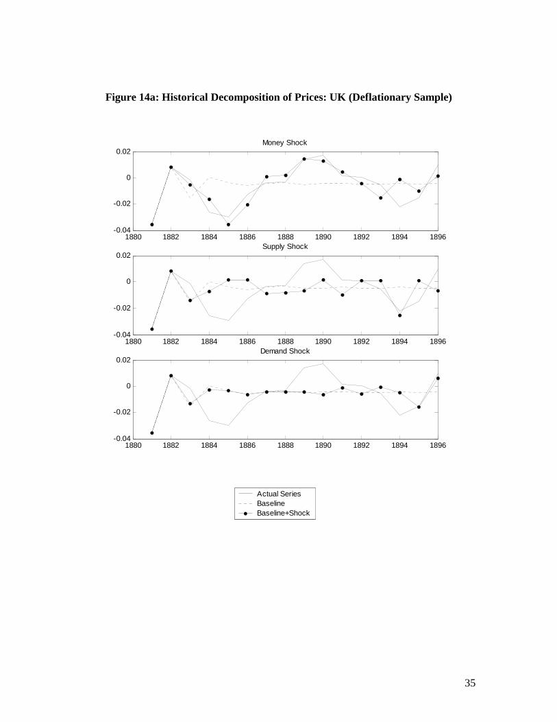
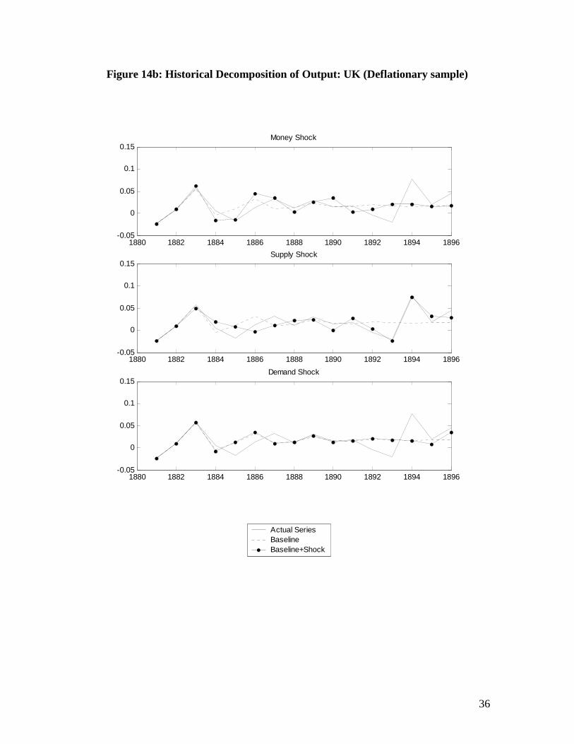
In all three countries the behaviour of the price level is driven by the money

shock. That is, while the impulse response functions show that supply shocks have short

run price effects, the quantitative impact of those effects is negligible. More germane to

our interests is the behaviour of output. In the UK and Germany supply shocks explain

virtually all output fluctuations. In the United States, supply shocks are the dominant

driving force, however, in a number of years money supply shocks have a noticeable

impact. This is consistent with the conventional wisdom that US monetary institutions

exacerbated output volatility in these periods. In all countries the impact of the demand

shocks was small.

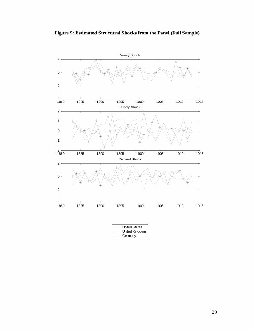
The estimated structural shocks are shown in Figure 9. Consistently with our

interpretation of the history of the period, the money supply shocks are correlated across

the three countries, as are the supply shocks. The demand shocks are uncorrelated,

suggesting that there was a significant idiosyncratic component to the temporary shocks.

Two sensitivity analyses were carried out to check the robustness of our results.

First we replaced M2 with M0, the monetary base, as our measure of money stock.

Second we included dummy variables for 1907 and 1908, a period of financial crisis for

the countries in our sample, in the VAR. In both cases, while the magnitudes of the

impulse response functions were slightly different, the qualitative results described above

remain. This was the case for the benchmark VAR for the entire period and the

subsequent VAR where we add in the world gold stock as an exogenous variable.

V. Deflationary Period Results

Using the panel consisting of the three core countries, a PVAR is estimated using

data from the period 1880-1896. This period saw a substantial price deflation as seen in

Figure 1. Taking into account the first three periods that are lost due to first differencing

the data and the two lags used in the PVAR, there are 14 observations for each country.

Clearly, this would not be enough data to estimate the VAR for each individual country

in the sample. However, in the PVAR data are pooled from the three countries in the

panel so that we have a total of 42 observations at our disposal. The test statistic of the

12

test of slope coefficient equality across countries is 35.75 with a p-value of 0.481 (see

Table 1). This means that there is no statistical evidence to suggest that we cannot pool

the data for the deflationary period.

We began by testing for the over-identifying restrictions in (5), and the results are

reported in Table 3. Similar to the full sample case we see that the test is rejected for the

US and is not rejected for Germany. However, for the UK the p-value is now 0.08. Using

the full sample in the PVAR the p-value for the UK was smaller than 0.001. Given that

the point estimate of the long run impact of money on output is similar, at about 0.5%,

the change in the p-value is most likely due to the smaller sample size, and hence larger

standard errors, rather than there being anything different for the UK in the deflationary

period. We therefore proceeded by estimating the model without monetary neutrality

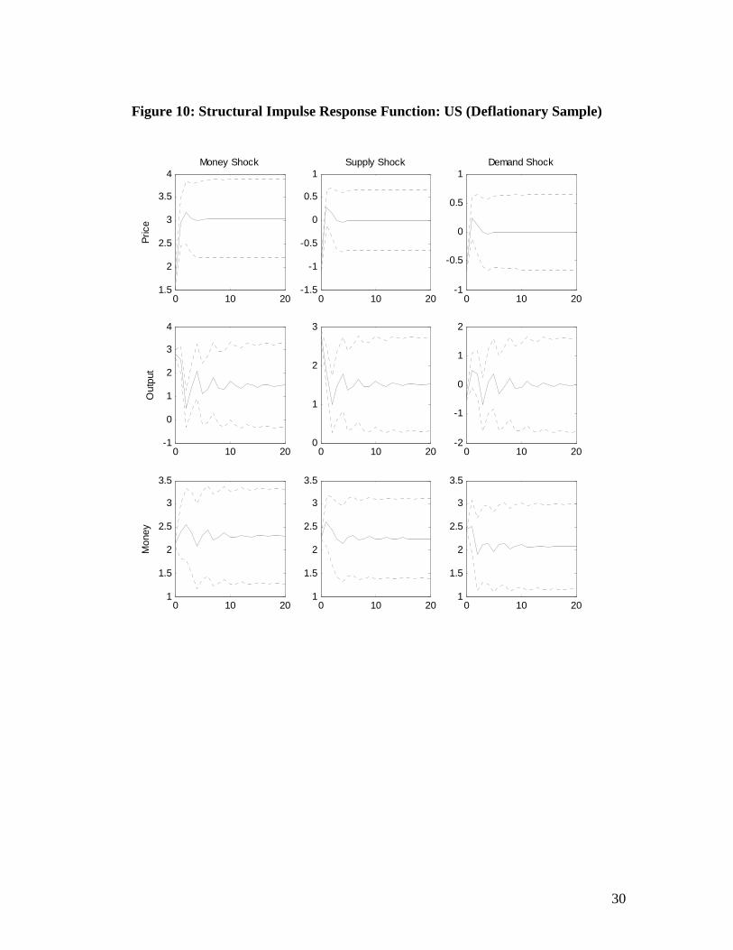
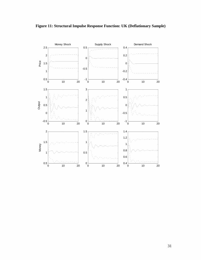
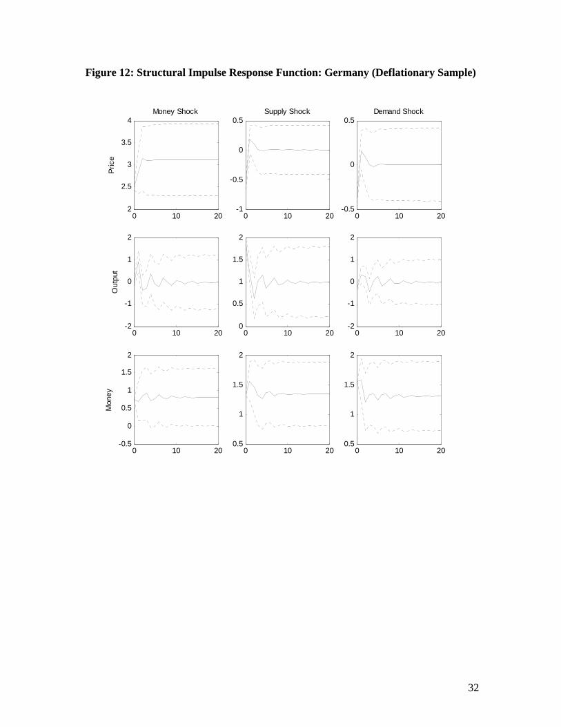
(that is, the model of equation (4)). Figures 10-12 report the structural impulse response

functions for each country.

Overall, the impulse response functions for the deflationary period have the same

qualitative appearance as in the full sample. In particular, for the US and UK the impulse

responses show that a money supply shock which has a given effect on the long run

money stock has the same estimated impact on output in both the full sample and the

deflationary sample. This is an implicit test of the symmetry of the responses in the

deflationary period and inflationary period, and suggests that, for the late nineteenth/early

twentieth period that we are examining, responses were symmetric in the two eras.

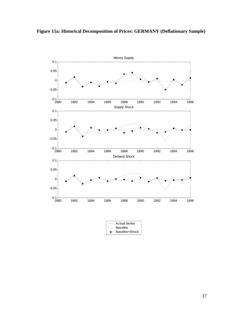
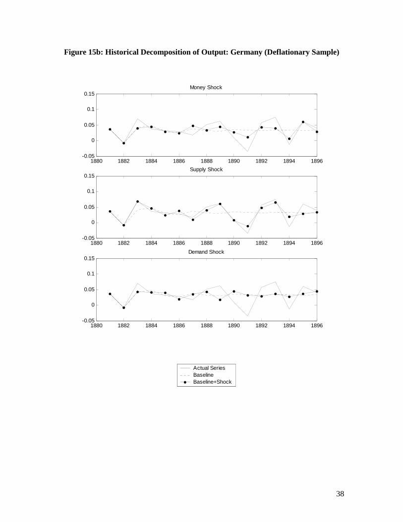
Finally the results of the historical decompositions of output are shown in Figures

13-15. While the sample sizes for the individual countries are small, it is clear for each

country that the behaviour of prices was driven by the money shock. That is, the deflation

of the late nineteenth century was generated by negative monetary shocks. The behaviour

of output is again largely driven by supply shocks, although in the mid-1880s US output

reflected the impact of all three types of shocks.

13

VI. Results for the full period with exogenous gold shocks

Our preferred identification, (5), is driven by the fact that during the period of our

sample, the countries in our panel were all on the gold standard. We are therefore

interested in knowing what role, if any, gold shocks played during this period. The model

that is estimated is

(9) ∑ ∑= =

−− +∆+∆++=∆p

j

m

kitktkjitjtiiit GoldyBDy

1 0189610 εγαα ,

where Goldt is the total world gold stock.8 In this specification gold is completely

exogenous to the system. As noted in Section 3, at very long horizons the world gold

stock may be endogenous, but given the time span of our data exogeneity is a reasonable

assumption. Table 4 shows the results of a Hausman type test for exogeneity. For all

countries and all variables we cannot reject the hypothesis that gold is exogenous to our

variables.9 A panel VAR is estimated using (9) with slope coefficients, Bj, and the impact

coefficients of gold, γj constrained to be equal across countries. Table 1 contains the

results of the Wald test that tests whether the coefficients on gold in (9) are common

across the countries in the panel. The reported p-value for this test is 0.63 so the

hypothesis that the gold coefficients are common across countries cannot be rejected.

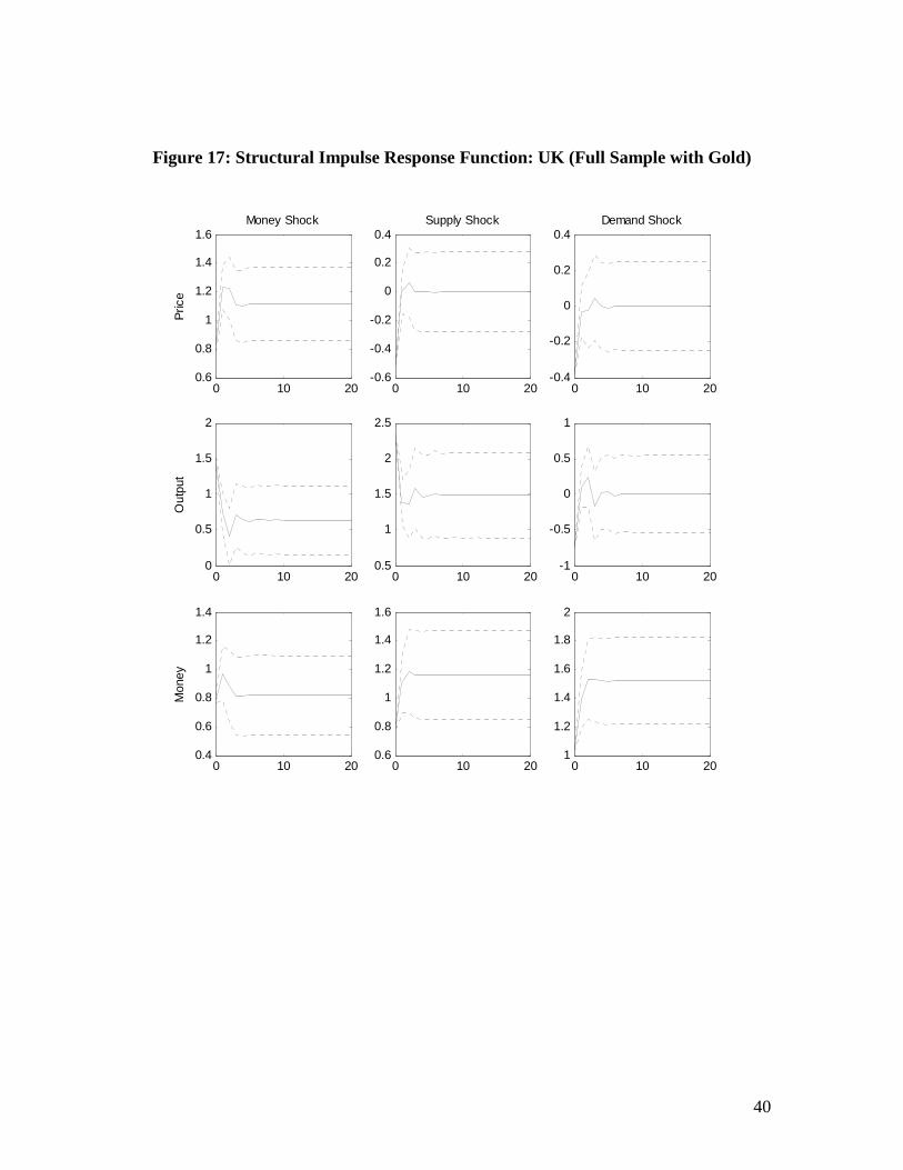
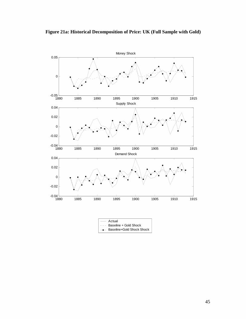
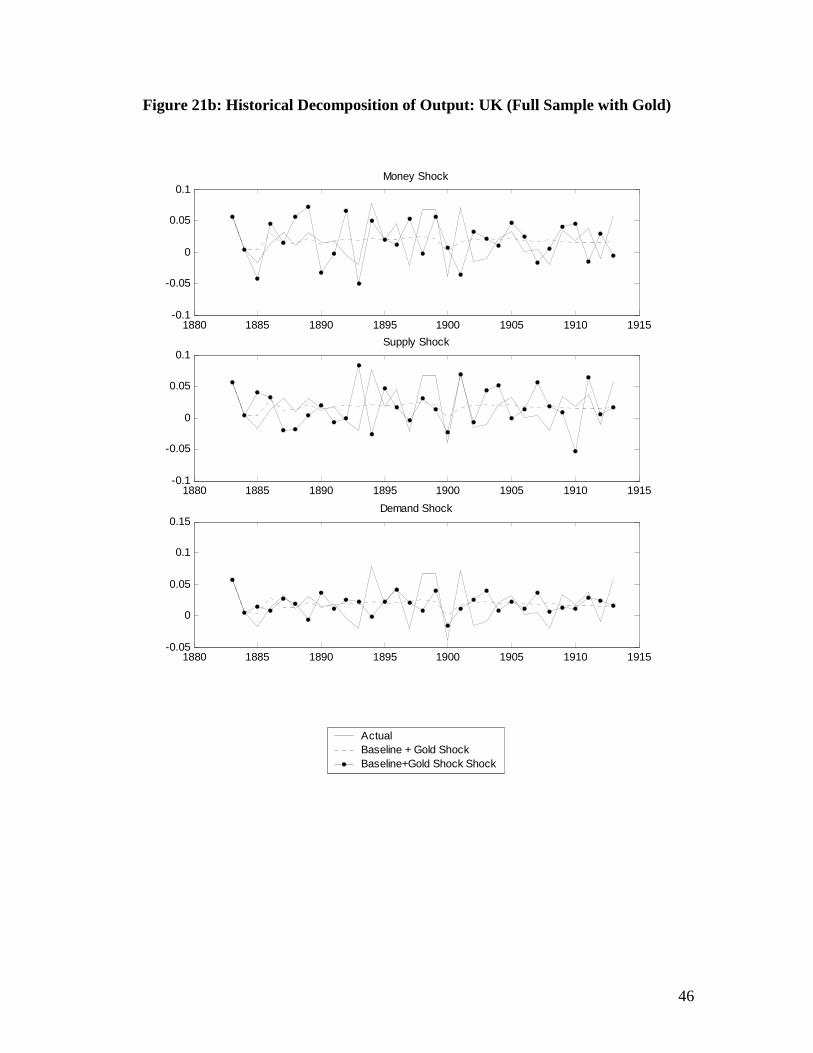
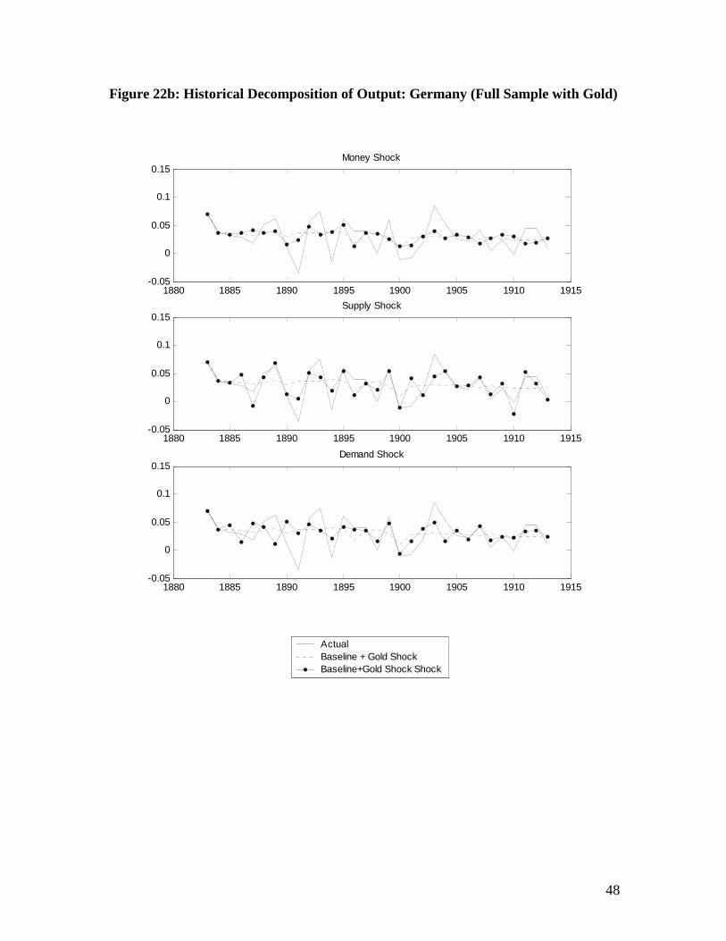
Figures 16 to 18 depict the structural impulse response functions calculated using

the estimates of (9). These figures are qualitatively similar to the previous impulse

response functions when gold was not included into the VAR.10 Figures 20 to 22 depict

the historical decompositions. Again we see that money contributes most to prices and

the supply shock explains most of the observed variation in output. It is interesting to

note that gold does not play an important role in the observed variation of prices and

output.

8 Gold data are from the US Gold Commission (1982), Vol. I Table SC-6. 9 Note that the Hausman test is really a test of whether ordinary least squares provide consistent estimates of (12). To conduct the Hausman test we use 2−∆ tgold as the instrument for tgold∆ . 10 The only qualitative difference is that the monetary shock has a small long run negative impact on German output (when we estimate over only the deflationary sample this result is overturned – see below).

14

We have also re-estimated the model for the deflation sample alone (1880-1896),

but for space reasons do not include the figures here.11 The historical decompositions for

prices show that, as in the case without gold, supply shocks and the non-monetary

demand shock contribute little to the behaviour of prices. But now the price level is

explained in part by gold shocks and in part by domestic money shocks. Gold shocks

however explain little of the output fluctuations.

Figure 19 shows the impact of a 1% increase in gold supply on prices, output and

money supply. We see that the long run impact of this gold shock is what we would

expect under the gold standard. That is, the long-run impact of a 1% increase in gold

supply is a 1% increase in prices, a 1% increase in money supply and no increase in

output. This result suggests that our assumptions based on the gold standard are not

unrealistic.

However, there is a puzzling result in that the initial impact of the gold shock on

prices is negative. One reason for this may be that the gold shocks that we are observing

could be price led rather than being exogenous to the system. That is, lower prices lead to

gold flows that appear in the data as positive gold supply shocks. This last observation

would suggest that gold is not entirely exogenous and the possible endogeneity between

price and gold should be modeled explicitly. How best to model this endogeneity is a

difficult question as gold supply most probably has an endogenous component and an

exogenous component. This problem is left for future research.

VII Conclusions

Inflation rates around the globe have fallen from historically high levels in the

1970s and 1980s to numbers close to zero as the 20th century ended. Indeed some

countries have experienced actual deflation. Yet output growth rates remain positive. Not

since the turn of the 19th century, have economies experienced such low inflation

associated with non-negative growth, and it seems natural to turn to that period to learn

about macro behaviour in low inflation or possibly deflationary environments.

11 Figures are available from the authors.

15

Deflation can reflect the impact of positive aggregate supply shocks (in the

absence of offsetting positive demand shocks) or negative demand shocks. In the latter

case, if the aggregate supply curve is non-vertical, the deflation will be ‘bad’ in that it

will be accompanied by negative output effects.

Our results show that the deflation in the late nineteenth century gold standard era

in three key countries reflected both positive aggregate supply and negative money

supply shocks. Yet the negative money shock had only a minor effect on output. This we

posit is because the aggregate supply curve was very steep in the short run. Thus our

empirical evidence suggests that deflation in the late nineteenth century was primarily

good.

Important issues for today’s environment arise from our findings. We need to be

clear about what was different between the late nineteenth century environment and that

of the twentieth and twenty first centuries. First, the historical era we analyze was the

classical gold standard regime under which all three countries were linked together via

common adherence to the gold standard convertibility rule and all faced a common

money shock – the vagaries of the gold standard.

Second, aggregate supply seems to have been an important source of the shocks

that we identify. This is likely in contrast to the other major deflationary episodes of the

the twentieth century including: 1920-21, 1929-33, and Japan in the 1990s, which many

observers posit reflected the consequences of severe monetary contraction.12 Today’s

environment in the US, Canada and the EU may indeed be closer to the pre-1914 era than

the earlier twentieth century episodes.

Third the short run aggregate supply seems to have been very steep pre-1913.

This meant that negative demand shocks did not have much of a contractionary bite. This

result is in sharp contrast to the experience of 1929-33. Many attribute the catastrophic

12 For a contrary view see Kehoe and Prescott (2002).

16

declines of output in the face of monetary contraction then to the presence of nominal

rigidities, in particular sticky wages (Bordo, Erceg and Evans, 2000).

Our analysis does not deal with many important issues that resonate in today’s

policy debate over what to do about the spectre of deflation. These include the zero

nominal bound problem -- that very low inflation by reducing nominal interest rates

makes it difficult to conduct monetary policy by conventional means (Orphanides, 2001).

In contrast to today, in the pre-1914 era, little emphasis was placed by the policy makers

in countries, like the UK and Germany, which had central banks, in using monetary

policy to stimulate the real economy. Hence the zero nominal bound was not viewed as a

problem.

We also do not explicitly distinguish between the effects of actual versus expected

price level changes. It is unexpected deflation that produces negative consequences.

However the steep slope of the aggregate supply curve revealed in our work suggests that

price level changes were large anticipated. We also do not consider the efficiency aspects

of deflation. According to Friedman (1969), the optimum holding of money would occur

at a rate of deflation equal to the long run growth rate of real output.

Finally, although we find that pre-1914 deflation was primarily of the good

variety, it doesn’t mean that people felt good about it. The common perception of the

1880s and 1890s in all three countries was that deflation was depressing. This in turn may

reflect the fact that deflation was largely unanticipated. It may also have reflected money

illusion.13 This was reflected in labor strife and political turbulence. This perception can

be seen in the views of US farmers who believed that the terms of trade had turned

against them and workers in all three countries who did not view falling money wages as

being compensated by even more rapidly falling commodity prices. It is doubtful if a true

deflation today would be any less unpopular.

13 Friedman and Schwartz ( 1963; 41-2) compare the U.S. experience of the 1870s when money growth exceeded the growth of the labor force but not the growth of real output so that nominal wages were rising, with the 1880s when money growth was less than the growth of the labor force and of real growth and money wages declined. They then relate these facts to the increase in labor unrest and agitation over the monetary standard.

17

Table 1: Test of Parameter Equality across Countries

Statistic p-value

Full Sample (1880-1913) 39.27 0.33 Deflationary Sample (1880-1896) 35.75 0.48

Gold Coefficients (Gold) 9.83 0.63 Table 2: Chow Test of Slope Parameter Stability between 1880-1896 and 1897-1913

Statistic p-value United States 21.18 0.270

United Kingdom 19.92 0.337 Germany 23.16 0.185

Panel(Full Sample) 15.23 0.646

Table 3: Test of Over-identifying Restrictions

United States United Kingdom Germany Statistic p-value Statistic p-value Statistic p-value

Single Equation 9.19 0.003 3.53 0.061 5.18 0.025 Panel (Full Sample) 33.66 0.000 14.07 0.000 0.192 0.661

Panel (Deflation Sample) 26.28 0.000 2.97 0.085 0.057 0.811

Table 4: Tests of Exogeneity of Gold

United States United Kingdom Germany Dependent variable Statistic p-value Statistic p-value Statistic p-value

Price 0.105 0.75 0.301 0.58 0.706 0.40 Output 0.108 0.74 0.018 0.89 0.483 0.49 Money 0.002 0.97 0.001 0.99 0.003 0.95

18

Figure 1: Data for Core Countries

1880 1885 1890 1895 1900 1905 1910 191570

80

90

100

110GDP Deflator: 1913=100

1880 1885 1890 1895 1900 1905 1910 191592

94

96

98

100log(real GDP): 1913 pounds (1913=100)

1880 1885 1890 1895 1900 1905 1910 191519

20

21

22

23log(money supply): pounds

United StatesUnited KingdomGermany

19

Figure 2: Gold Production: 1873-1913

1870 1875 1880 1885 1890 1895 1900 1905 1910 19154

6

8

10

12

14

16

18

20

22

24

Year

milli

on fi

ne o

z's

20

Figure 314: Structural Impulse Response Functions: United States (Full Sample)

0 10 201.5

2

2.5

3

3.5

4Money Shock

Pric

e

0 10 20-1

-0.5

0

0.5Supply Shock

0 10 20-1

-0.5

0

0.5

1Demand Shock

0 10 200

1

2

3

Out

put

0 10 201

1.5

2

2.5

3

3.5

0 10 20-2

-1

0

1

2

0 10 202

2.5

3

3.5

4

Mon

ey

0 10 201.5

2

2.5

3

0 10 201.5

2

2.5

3

3.5

14 The y-axis for all impulse response functions are measured in percentage points.

21

Figure 4: Structural Impulse Response Functions: United Kingdom (Full Sample)

0 10 200.8

1

1.2

1.4

1.6Money Shock

Pric

e

0 10 20-0.6

-0.4

-0.2

0

0.2

0.4Supply Shock

0 10 20-0.4

-0.2

0

0.2

0.4Demand Shock

0 10 20-0.5

0

0.5

1

1.5

Out

put

0 10 200.5

1

1.5

2

2.5

3

0 10 20-1

-0.5

0

0.5

1

0 10 200.4

0.6

0.8

1

1.2

1.4

Mon

ey

0 10 200.6

0.8

1

1.2

1.4

1.6

0 10 201

1.2

1.4

1.6

1.8

2

22

Figure 5: Structural Impulse Response Functions: Germany (Full Sample)

0 10 201.5

2

2.5

3Money Shock

Pric

e

0 10 20-0.6

-0.4

-0.2

0

0.2

0.4Supply Shock

0 10 20-1

-0.5

0

0.5Demand Shock

0 10 20-1

-0.5

0

0.5

1

Out

put

0 10 200.5

1

1.5

2

2.5

0 10 20-1

-0.5

0

0.5

1

0 10 200

0.5

1

1.5

2

Mon

ey

0 10 200.8

1

1.2

1.4

1.6

0 10 201.5

2

2.5

3

23

Figure 6a: Historical Decomposition of Prices: US (Full Sample)

1880 1885 1890 1895 1900 1905 1910 1915-0.1

-0.05

0

0.05

0.1

Money Shock

1880 1885 1890 1895 1900 1905 1910 1915-0.1

-0.05

0

0.05

0.1

Supply Shock

1880 1885 1890 1895 1900 1905 1910 1915-0.1

-0.05

0

0.05

0.1

Demand Shock

Actual SeriesBaselineBaseline+Shock

24

Figure 6b: Historical Decomposition of Output: US (Full Sample)

1880 1885 1890 1895 1900 1905 1910 1915-0.1

0

0.1

0.2

0.3Money Shock

1880 1885 1890 1895 1900 1905 1910 1915-0.1

0

0.1

0.2

0.3Supply Shock

1880 1885 1890 1895 1900 1905 1910 1915-0.1

0

0.1

0.2

0.3Demand Shock

Actual SeriesBaselineBaseline+Shock

25

Figure 7a: Historical Decomposition of Prices: UK (Full Sample)

1880 1885 1890 1895 1900 1905 1910 1915-0.04

-0.02

0

0.02

0.04Money Shock

1880 1885 1890 1895 1900 1905 1910 1915-0.04

-0.02

0

0.02

0.04Supply Shock

1880 1885 1890 1895 1900 1905 1910 1915-0.04

-0.02

0

0.02

0.04Demand Shock

Actual SeriesBaselineBaseline+Shock

26

Figure 7b: Historical Decomposition of Output: UK (Full Sample)

1880 1885 1890 1895 1900 1905 1910 1915-0.05

0

0.05

0.1

0.15Money Shock

1880 1885 1890 1895 1900 1905 1910 1915-0.05

0

0.05

0.1

0.15Supply Shock

1880 1885 1890 1895 1900 1905 1910 1915-0.05

0

0.05

0.1

0.15Demand Shock

Actual SeriesBaselineBaseline+Shock

27

Figure 8a: Historical Decomposition of Prices: Germany (Full Sample)

1880 1885 1890 1895 1900 1905 1910 1915-0.1

-0.05

0

0.05

0.1Money Shock

1880 1885 1890 1895 1900 1905 1910 1915-0.1

-0.05

0

0.05

0.1Supply Shock

1880 1885 1890 1895 1900 1905 1910 1915-0.1

-0.05

0

0.05

0.1Demand Shock

Actual SeriesBaselineBaseline+Shock

28

Figure 8b: Historical Decomposition of Output: Germany (Full Sample)

1880 1885 1890 1895 1900 1905 1910 1915-0.1

0

0.1

0.2Money Shock

1880 1885 1890 1895 1900 1905 1910 1915-0.1

0

0.1

0.2Supply Shock

1880 1885 1890 1895 1900 1905 1910 1915-0.1

0

0.1

0.2Demand Shock

Actual SeriesBaselineBaseline+Shock

29

Figure 9: Estimated Structural Shocks from the Panel (Full Sample)

1880 1885 1890 1895 1900 1905 1910 1915-4

-2

0

2Money Shock

1880 1885 1890 1895 1900 1905 1910 1915-2

-1

0

1

2Supply Shock

1880 1885 1890 1895 1900 1905 1910 1915-4

-2

0

2Demand Shock

United StatesUnited KingdomGermany

30

Figure 10: Structural Impulse Response Function: US (Deflationary Sample)

0 10 201.5

2

2.5

3

3.5

4Money Shock

Pric

e

0 10 20-1.5

-1

-0.5

0

0.5

1Supply Shock

0 10 20-1

-0.5

0

0.5

1Demand Shock

0 10 20-1

0

1

2

3

4

Out

put

0 10 200

1

2

3

0 10 20-2

-1

0

1

2

0 10 201

1.5

2

2.5

3

3.5

Mon

ey

0 10 201

1.5

2

2.5

3

3.5

0 10 201

1.5

2

2.5

3

3.5

31

Figure 11: Structural Impulse Response Function: UK (Deflationary Sample)

0 10 200.5

1

1.5

2

2.5Money Shock

Pric

e

0 10 20-1

-0.5

0

0.5Supply Shock

0 10 20-0.4

-0.2

0

0.2

0.4Demand Shock

0 10 20-0.5

0

0.5

1

1.5

Out

put

0 10 200

1

2

3

0 10 20-1

-0.5

0

0.5

1

0 10 200.5

1

1.5

2

Mon

ey

0 10 200

0.5

1

1.5

0 10 200.4

0.6

0.8

1

1.2

1.4

32

Figure 12: Structural Impulse Response Function: Germany (Deflationary Sample)

0 10 202

2.5

3

3.5

4Money Shock

Pric

e

0 10 20-1

-0.5

0

0.5Supply Shock

0 10 20-0.5

0

0.5Demand Shock

0 10 20-2

-1

0

1

2

Out

put

0 10 200

0.5

1

1.5

2

0 10 20-2

-1

0

1

2

0 10 20-0.5

0

0.5

1

1.5

2

Mon

ey

0 10 200.5

1

1.5

2

0 10 200.5

1

1.5

2

33

Figure 13a:Historical Decomposition of Prices: US (Deflationary Sample)

1880 1882 1884 1886 1888 1890 1892 1894 1896-0.1

-0.05

0

0.05

0.1

Money Shock

1880 1882 1884 1886 1888 1890 1892 1894 1896-0.1

-0.05

0

0.05

0.1

Supply Shock

1880 1882 1884 1886 1888 1890 1892 1894 1896-0.1

-0.05

0

0.05

0.1

Demand Shock

Actual SeriesBaselineBaseline+Shock

34

Figure 13b: Historical Decomposition of Output: US (Deflationary Sample)

1880 1882 1884 1886 1888 1890 1892 1894 1896-0.1

0

0.1

0.2

0.3Money Shock

1880 1882 1884 1886 1888 1890 1892 1894 1896-0.1

0

0.1

0.2

0.3Supply Shock

1880 1882 1884 1886 1888 1890 1892 1894 1896-0.1

0

0.1

0.2

0.3Demand Shock

Actual SeriesBaselineBaseline+Shock

35

Figure 14a: Historical Decomposition of Prices: UK (Deflationary Sample)

1880 1882 1884 1886 1888 1890 1892 1894 1896-0.04

-0.02

0

0.02Money Shock

1880 1882 1884 1886 1888 1890 1892 1894 1896-0.04

-0.02

0

0.02Supply Shock

1880 1882 1884 1886 1888 1890 1892 1894 1896-0.04

-0.02

0

0.02Demand Shock

Actual SeriesBaselineBaseline+Shock

36

Figure 14b: Historical Decomposition of Output: UK (Deflationary sample)

1880 1882 1884 1886 1888 1890 1892 1894 1896-0.05

0

0.05

0.1

0.15Money Shock

1880 1882 1884 1886 1888 1890 1892 1894 1896-0.05

0

0.05

0.1

0.15Supply Shock

1880 1882 1884 1886 1888 1890 1892 1894 1896-0.05

0

0.05

0.1

0.15Demand Shock

Actual SeriesBaselineBaseline+Shock

37

Figure 15a: Historical Decomposition of Prices: GERMANY (Deflationary Sample)

1880 1882 1884 1886 1888 1890 1892 1894 1896-0.1

-0.05

0

0.05

0.1Money Supply

1880 1882 1884 1886 1888 1890 1892 1894 1896-0.1

-0.05

0

0.05

0.1Supply Shock

1880 1882 1884 1886 1888 1890 1892 1894 1896-0.1

-0.05

0

0.05

0.1Demand Shock

Actual SeriesBaselineBaseline+Shock

38

Figure 15b: Historical Decomposition of Output: Germany (Deflationary Sample)

1880 1882 1884 1886 1888 1890 1892 1894 1896-0.05

0

0.05

0.1

0.15Money Shock

1880 1882 1884 1886 1888 1890 1892 1894 1896-0.05

0

0.05

0.1

0.15Supply Shock

1880 1882 1884 1886 1888 1890 1892 1894 1896-0.05

0

0.05

0.1

0.15Demand Shock

Actual SeriesBaselineBaseline+Shock

39

Figure 16: Structural Impulse Response Function: US (Full Sample with Gold)

0 10 201.5

2

2.5

3

3.5

4Money Shock

Pric

e

0 10 20-1

-0.5

0

0.5Supply Shock

0 10 20-1

-0.5

0

0.5

1Demand Shock

0 10 200

1

2

3

4

Out

put

0 10 201

1.5

2

2.5

3

3.5

0 10 20-2

-1

0

1

2

0 10 202.5

3

3.5

4

4.5

Mon

ey

0 10 201.5

2

2.5

3

0 10 201.5

2

2.5

3

3.5

40

Figure 17: Structural Impulse Response Function: UK (Full Sample with Gold)

0 10 200.6

0.8

1

1.2

1.4

1.6Money Shock

Pric

e

0 10 20-0.6

-0.4

-0.2

0

0.2

0.4Supply Shock

0 10 20-0.4

-0.2

0

0.2

0.4Demand Shock

0 10 200

0.5

1

1.5

2

Out

put

0 10 200.5

1

1.5

2

2.5

0 10 20-1

-0.5

0

0.5

1

0 10 200.4

0.6

0.8

1

1.2

1.4

Mon

ey

0 10 200.6

0.8

1

1.2

1.4

1.6

0 10 201

1.2

1.4

1.6

1.8

2

41

Figure 18: Structural Impulse Response Function: Germany (Full Sample with Gold)

0 10 201.5

2

2.5

3Money Shock

Pric

e

0 10 20-0.6

-0.4

-0.2

0

0.2

0.4Supply Shock

0 10 20-0.6

-0.4

-0.2

0

0.2

0.4Demand Shock

0 10 20-1.5

-1

-0.5

0

0.5

Out

put

0 10 200.5

1

1.5

2

2.5

0 10 20-1.5

-1

-0.5

0

0.5

1

0 10 200

0.5

1

1.5

Mon

ey

0 10 200.6

0.8

1

1.2

1.4

0 10 201

1.5

2

2.5

3

42

Figure 19: Impulse Response to a 1% Increase in Gold

0 2 4 6 8 10 12 14 16 18 20-2

-1

0

1

2

3P

rice

0 2 4 6 8 10 12 14 16 18 20-1

0

1

2

3

4

5

Out

put

0 2 4 6 8 10 12 14 16 18 20-1

0

1

2

3

4

Mon

ey

43

Figure 20a: Historical Decomposition of Price: US (Full Sample with Gold)

1880 1885 1890 1895 1900 1905 1910 1915-0.1

-0.05

0

0.05

0.1Money Shock

1880 1885 1890 1895 1900 1905 1910 1915-0.1

-0.05

0

0.05

0.1Supply Shock

1880 1885 1890 1895 1900 1905 1910 1915-0.1

-0.05

0

0.05

0.1Demand Shock

ActualBaseline + Gold ShockBaseline+Gold Shock Shock

44

Figure 20b: Historical Decomposition of Output: US (Full Sample with Gold)

1880 1885 1890 1895 1900 1905 1910 1915-0.1

0

0.1

0.2Money Shock

1880 1885 1890 1895 1900 1905 1910 1915-0.1

0

0.1

0.2Supply Shock

1880 1885 1890 1895 1900 1905 1910 1915-0.1

0

0.1

0.2Demand Shock

ActualBaseline + Gold ShockBaseline+Gold Shock Shock

45

Figure 21a: Historical Decomposition of Price: UK (Full Sample with Gold)

1880 1885 1890 1895 1900 1905 1910 1915-0.05

0

0.05Money Shock

1880 1885 1890 1895 1900 1905 1910 1915-0.04

-0.02

0

0.02

0.04Supply Shock

1880 1885 1890 1895 1900 1905 1910 1915-0.04

-0.02

0

0.02

0.04Demand Shock

ActualBaseline + Gold ShockBaseline+Gold Shock Shock

46

Figure 21b: Historical Decomposition of Output: UK (Full Sample with Gold)

1880 1885 1890 1895 1900 1905 1910 1915-0.1

-0.05

0

0.05

0.1Money Shock

1880 1885 1890 1895 1900 1905 1910 1915-0.1

-0.05

0

0.05

0.1Supply Shock

1880 1885 1890 1895 1900 1905 1910 1915-0.05

0

0.05

0.1

0.15Demand Shock

ActualBaseline + Gold ShockBaseline+Gold Shock Shock

47

Figure 22a: Historical Decomposition of Price: Germany (Full Sample with Gold)

1880 1885 1890 1895 1900 1905 1910 1915-0.1

-0.05

0

0.05

0.1Money Shock

1880 1885 1890 1895 1900 1905 1910 1915-0.1

-0.05

0

0.05

0.1Supply Shock

1880 1885 1890 1895 1900 1905 1910 1915-0.1

-0.05

0

0.05

0.1Demand Shock

ActualBaseline + Gold ShockBaseline+Gold Shock Shock

48

Figure 22b: Historical Decomposition of Output: Germany (Full Sample with Gold)

1880 1885 1890 1895 1900 1905 1910 1915-0.05

0

0.05

0.1

0.15Money Shock

1880 1885 1890 1895 1900 1905 1910 1915-0.05

0

0.05

0.1

0.15Supply Shock

1880 1885 1890 1895 1900 1905 1910 1915-0.05

0

0.05

0.1

0.15Demand Shock

ActualBaseline + Gold ShockBaseline+Gold Shock Shock

49

References Amisano, G. and C. Giannini, (1997) Topics in Structural VAR Econometrics, Springer-Verlag, Berlin. Balke, N. and R. Gordon (1986) “Historical Data” in Robert J. Gordon, ed., The American Business Cycle, Chicago: University of Chicago Press. Barro, R. (1979) “Money and the Price Level under the Gold Standard” Economic Journal, March (89): 13-33. Bergman, U., M. Bordo, and L. Jonung (1998), “Historical Evidence on Business Cycles: The International Experience” in J. Fuhrer and S. Schuh eds., Federal Reserve Bank of Boston Conference Series, Beyond Shocks: What causes Business Cycles? (42), 65-113. Bernanke, B. (1983), “Nonmonetary effects of the Financial Crisis in Propagation of the Great Depression,” American Economic Review, 73(3): 257-76. Blanchard, O.J. and Quah, D. (1989), “The Dynamic Effect of Aggregate Demand and Supply Disturbances,” American Economic Review, 79(4), 655-673. Bordo, M. (1981), “The Classical Gold standard: Some lessons for today,” Federal Reserve Bank of St. Louis Review, 63(5): 2-17. Bordo, M. and R. W. Ellson, (1985) “A Model of the Classical Gold Standard with depletion” Journal of Monetary Economics (16): 109-20. Bordo, M., C. Erceg and C. Evans (2000) “Money, Sticky Wages and the Great Depression,” American Economic Review, 90(5), 1447-63. Bordo, M. and A. Redish (2004) “Is Deflation Depressing?” in Richard Burdekin and Pierre Siklos ( eds) Deflation: Current and Historical Perspectives. New York: Cambridge University Press. (in press) Borio and Filardo (2003)" Back to the Future? Assessing the Threat of Deflation" Bank for International Settlements. Basle April. Canova, F. and M. Ciccarealli, (1999) “Forecasting and Turning Point Predictions in a Bayesian Panel VAR Model,” mimeo. Craig, L. and D. Fisher (2000), The European Macroeconomy: Growth and integration, 1500-1913, London: Edward Elgar. Deutsche Bundesbank (1976) Deutsches Geld- und Bankwesen in Zahlen, 1876-1975, Frankfurt: Herausgeber Deutsche Bundesbank.

50

Dowd, K. and D. Chappell, (1997) “A Simple Model of the Gold Standard” Journal of Money Credit and Banking (29:1): 94-105. Friedman, M. (1969) “The Optimum Quantity of Money” Milton Friedman, The Optimum Quantity of Money and other Essays. Chicago: Aldine Publishers. Holtz-Eakin, D., W. Newey, and H.S. Rosen, (1988) “Estimating Vector Autoregressions with Panel Data,” Econometrica, 56(6), 1371-1395. IMF (2002) “Chapter 3: Recessions and Recoveries”, World Economic Outlook Kehoe, T. and E. Prescott, (2002) “Great Depressions of the 20th century,” Review of Economic Dynamics, 5(1): 1-18. Kumar, Mannohan, S. Taimur Baig, Jorg Decressin, Chris Faulkner-MacDanagh and Tarhan Feyziogulu (2003) “Deflation: Determinants, Risks, and Policy Options.” IMF Occasional Paper #221. McCloskey, D. and J. R. Zecher (1976) “How the gold standard worked, 1880-1913” in J. A. Frenkel and H.G. Johnson, eds., The Monetary Approach to the Balance of Payments, Toronto: University of Toronto Press. Mitchell, B. (1998) International Historical Statistics: Europe, 1750-1993 4th edn. New York: Stockton Press. Orphanides, A. (2001) “Monetary Policy rules, macroeconomic stability and inflation: A view from the trenches.” Federal Reserve Board of Governors. Finance and Economics Discussion paper 2001-62. Pesaran, M.H. and R. Smith, (1995) “Estimating Long-Run Relationships from Dynamic Heterogeneous Panels,” Journal of Econometrics, 68, 78-113. Rockoff, H. (1984) “Some Evidence on the Real Price of Gold, Its Costs of Production, and Commodity Prices” in M.D. Bordo and A. J. Schwartz, A Retrospective on the Classical Gold Standard, 1821-1931 Chicago: University of Chicago Press. Sommariva, A. and G. Tullio, (1987) German macroeconomic history, 1880-1970: A study of the effects of economic policy on inflation, currency depreciation and growth, New York: St Martin’s Press. United States Gold Commission (1982) Report to the Congress of the Commision on the Role of Gold in the Domestic and International Monetary Systems. Washington DC March.