NBER WORKING PAPER SERIES

A CUSTOMS UNION WITH MULTINATIONAL FIRMS:THE AUTOMOBILE MARKET IN ARGENTINA AND BRAZIL

Irene Brambilla

Working Paper 11745http://www.nber.org/papers/w11745

NATIONAL BUREAU OF ECONOMIC RESEARCH1050 Massachusetts Avenue

Cambridge, MA 02138November 2005

I am grateful to my advisors Gene Grossman, Bo Honoré, and Elie Tamer for their guidance and suggestions.I also wish to thank Steve Berry, Don Davis, Penny Goldberg, Han Hong, Giovanni Maggi, Guido Porto, andseminar participants at Chicago GSB, Columbia, Georgetown, Harvard, the NBER Summer Institute, NYU,NYU Stern, Princeton, Santa Cruz, Texas-Austin, Toronto, di Tella, The World Bank, and Yale for manyhelpful comments. All errors are mine. email: irene.brambilla@yale.edu. 37 Hillhouse, P.O. Box 208264,New Haven, CT 06520-8264 The views expressed herein are those of the author(s) and do not necessarilyreflect the views of the National Bureau of Economic Research.

©2005 by Irene Brambilla. All rights reserved. Short sections of text, not to exceed two paragraphs, maybe quoted without explicit permission provided that full credit, including © notice, is given to the source.

A Customs Union with Multinational Firms: The Automobile Market in Argentina and BrazilIrene BrambillaNBER Working Paper No. 11745November 2005JEL No. F12, F13, F15

ABSTRACTThis paper looks empirically into the behavior of multinational firms in international oligopolistic

markets with trade balance constraints. I show how a particular form of non-tariff barrier applied at

the firm level can lead to an increase in trade flows in the presence of intra-firm strategic trade. In

my application, I estimate a model of demand, supply and trade policy in the automobile sector in

Argentina and Brazil during 1996-1999.

I measure the economic impact of a trade balance constraint that was in effect during that period and

I compute predicted economic outcomes for the full adoption of a customs union, as has been agreed

as part of the Mercosur negotiations, separating the sometimes opposing impacts of the removal of

non-tariff barriers and the adoption of a common external tariff. Results show that the elimination

of non-tariff barriers dominates the leveling of tariffs. Imports from outside of Mercosur increase

under the new regime even though tariffs against these goods become more discriminatory, and

exports from Brazil to Argentina decrease once the trade balance constraint is removed.

Irene BrambillaYale UniversityDepartment of Economics37 HilllhouseP. O. Box 208264New Haven, CT 06520-8264and NBERirene.brambilla@yale.edu

1 Introduction

This paper looks empirically into the behavior of multinational firms in international oligopolistic

markets with trade balance constraints. I show how a particular form of non-tariff barrier applied

at the firm level can lead to an increase in trade flows in the presence of intra-firm strategic trade.

In my application, I estimate a model of demand, supply and trade policy in the automobile sector

in Argentina and Brazil during 1996-1999. I measure the economic impact of a trade balance

constraint that was in effect during that period and I compute predicted economic outcomes for

the full adoption of a customs union, as it has been agreed as part of the Mercosur negotiations.

Argentina, Brazil, Uruguay and Paraguay formed a customs union - Mercosur - in 1995. The

inclusion of the automobile sector was initially negotiated for 2000, with programmed tariff and

non-tariff barriers (NTBs) phase-outs during 1996-1999. The complete elimination of the NTBs

was later postponed until 2006.

During the period 1996-1999, there were two non-tariff barriers in place both from the Argentine

and from the Brazilian sides: there was a quota on bilateral net imports, and there was a trade

balance constraint on global trade. Both of these restrictions were applied to each car manufacturer

in each of the two countries. The trade balance requirement restricted the value of imports of a

particular firm to be less or equal to the value of its exports plus some additional export credits.

Both imports and exports from the partner (Argentina and Brazil) and from other countries were

included in the trade balance requirement.

I model the behavior of the car manufacturers in Argentina and Brazil and incorporate the

effects of tariffs and NTBs into their price decision making. I first show that the effect of the trade

balance constraint is qualitatively not determined. The combination of trade balance constraints

with strategic intra-firm trade can lead to artificially high bilateral trade. The reason is that a given

firm needs to satisfy the constraints in both countries and can use bilateral trade as an instrument

to increase exports in the country where they are most needed. When NTBs are eliminated, the

directions of change in bilateral flows are a priori unpredictable. The evaluation of the effect of

trade balance constraint on trade flows shades light both on the behavior of multinational firms

under this particular trade policy and on the direction in which trade is going to move after the

customs union is fully adopted.

In addition, the Mercosur negotiations involve the adoption of a common external tariff which is

higher than the average tariffs in Argentina and Brazil during 1996-1999. Thus, the customs union

1

agreement involves two opposing changes in trade policy that have an impact on external imports:

the increase in the external tariff - which favors imports from the partners and domestic production

in detriment of imports from other countries - and the removal of the trade balance constraint -

which leads to an increase in external imports. Whether the trade diverting effect of the increase

in the tariff level is more than compensated by the trade creating effect from eliminating the trade

balance constraint is again an empirical question.

I estimate the imposed cost of the NTBs and simulate a counterfactual equilibrium in which

the NTBs are removed and the common external tariff is adopted. By comparing the observed

and predicted equilibrium outcomes during 1996-1999, I asses the impact of the customs union

on prices, trade flows, revenue, profits and welfare. Moreover, by computing an intermediate

equilibrium without NTBs but with the different tariff levels that were in effect during 1996-1999,

I decompose the effects of the two policy changes.

I find that the elimination of non-tariff barriers dominates the levelling of tariffs for all the

effects that I measure. In particular, imports from outside of Mercosur increase under the new

regime even though tariffs against these goods become more discriminatory. Another finding is

that the trade balance constraint imposes a higher cost to Brazilian subsidiaries relative to their

Argentine counterparts leading to excessive exports from Brazil to Argentina. Hence, under the

customs union regime, exports from Brazil to Argentina are predicted to decrease.

Previous evaluations of trade policy in automobile markets have looked at the voluntary export

restraint (VER) of Japanese vehicles exported to the U.S. that was set up in 1981. Dixit (1988)

calibrates a model with two differentiated products, American and Japanese. He computes the

optimal tariff on cars and finds that restricting Japanese imports, by means of a higher tariff,

would have been welfare enhancing for the U.S.. Feenstra (1984) and (1988) estimates the increase

in prices of Japanese cars that was due to the VER. He shows that part of the increase in prices

is explained by an upgrade in quality. Goldberg (1995) estimates a structural model of supply and

demand in the U.S. market and simulates the counterfactual equilibrium without the VER. Berry,

Levinsohn and Pakes (1999) run a similar exercise with a different demand specification. Verboven

(1996) and Goldberg and Verboven (2001) estimate structural models of supply and demand in the

European car market and indirectly focus on restrictions to Japanese car model in the context of

the study of price discrimination and price dispersion across several European countries.

The empirical strategy that I adopt is very similar in spirit to Goldberg (1995) and Berry,

2

Levinsohn and Pakes (1999). The estimation method consists on specifying a full structural model

of the behavior of the firms - including the choice variables, the nature of the competition and other

factors influencing the market - which can be summarized by a system of first order conditions. Such

system includes prices, marginal costs, costs imposed by trade policy, and a demand function and

price derivatives (or elasticities). If prices, quantities and price derivatives are observed, the cost of

each differentiated product can be estimated by finding the values of the cost that satisfy the system

of first order conditions. Firms choose prices (or quantities) given a demand function and marginal

costs; the researcher works backwards, given the observed prices and the demand function, the

marginal cost that generated those decisions can be recovered. In practice, the demand functions

are not observed and need to be estimated, either as a first step or jointly with the supply side.

The recovered marginal costs reflect both the cost of production and the costs imposed by

trade policy and it is necessary to disentangle the two of them to be able to run a counterfactual

exercise that involves a change in trade policy. The previous structural studies specify a parametric

functional form for the cost function in which the production cost depends on physical attributes

of the automobiles. Instead of estimating the production cost of each car directly, they reduce

the number of parameters by estimating the coefficients of a cost function (plus the trade policy

parameters). This procedure imposes further functional forms assumptions on a method that is

already substantially relying on structure.

In my application, I estimate a model of supply and trade policy in the automobile sector in

two countries - Argentina and Brazil. Since automobile firms are subsidiaries of multinational

corporations, the same agents are located in the two countries and maximize profits jointly in the

two markets. In terms of the estimation method, this translates into observing two sets of quantities,

prices and demand derivatives (one in Argentina and one in Brazil) while only one marginal costs

for each model (since each model is produced in only one country). I develop a minimum distance

estimator that takes advantage of the additional information from multiple equilibrium outcomes

(in this case two) and allows me to estimate the production cost and the trade policy parameters

directly from the behavior of firms, without imposing functional form assumptions on costs of

production.

This approach is suitable for applications in which there are data of product sales and prices

on more than one market but only one production cost. It is natural to apply the procedure

to trade models - as in Verboven (1996) and Goldberg and Verboven (2001),- it is also suitable

3

for closed-economy industrial organization applications with demand and price data on different

jurisdictions.

On the demand side, I adopt the random coefficients model of Berry (1994) and Berry, Levinsohn

and Pakes (1995). The procedure to estimate the supply side, however, is independent of the chosen

demand model.

In Section 2, I describe the characteristics of the automobile market in Argentina and Brazil

including the trade policy. In Section 3, I formalize the description of the industry into a model

of oligopoly with differentiated products. The estimation details of the supply side can be found

in Section 4. Section 5 describes the data and the results of the estimation both of supply and

demand parameters. Section 6 presents the description and results of the counterfactual adoption

of a customs union as has been scheduled for 2006.

2 Automobile market and trade policy

Automobiles are produced in Argentina and Brazil by subsidiaries of multinational corporations,

most of them associated with local investors. The firms located in the area are Ford, General Motors,

Chrysler, Fiat, Volkswagen, Mercedes Benz, Peugeot-Citroen, Renault, Toyota and Honda.1 There

are no purely domestic firms, and the participation of local capital in the joint ventures with

multinationals is minoritarian.

All these firms have production facilities in both countries. Renault, Toyota and

Peugeot-Citroen have regional headquarters in Argentina, while the remaining firms are primarily

based in Brazil. Generally, the car models produced in Argentina are different from the models

produced in Brazil. In some cases, there are overlaps of the main production lines across the two

countries but the models maintain some distinctive features such as different engine size or number

of doors. For example, between 1996 and 1997, Honda manufactured the Accord in Argentina and

the Civic in Brazil (different production lines); while between 1996 and 1999, Ford produced the

Escort in Argentina with the exception of the 1,000cc engine size version, that was produced in

Brazil (same production line but different final models).

Firms trade models between Argentina and Brazil and also import and export from and to other

countries. The largest fraction of trade is bilateral. Other export destinations are Latin America

and Europe, primarily Italy and France, although this varies substantially by year. Cars produced1Chrysler and Mercedes Benz merged in 2000 and formed Daimler-Chrysler

4

in Argentina and Brazil are mostly compact, small and medium sized, while models imported from

other countries include larger vehicles and SUVs. Brazil tends to specialize in smaller models than

Argentina. Trade in finished vehicles is a large fraction of bilateral trade. For example, in 1997,

imports of cars accounted for more than 17% of Brazilian imports from Argentina, and 10% of

Argentine imports from Brazil.

There are also car manufacturers that do not have production facilities in the area and whose

cars are only available in Argentina and Brazil through imports. The most important among these

corporations in terms of sales during the second half of the 1990’s are Rover, Isuzu and Daewoo.

These firms are subject to a different -more restrictive- trade regime in both countries and account

for less than 10 percent of domestic sales in Argentina and Brazil. Throughout this paper, I focus on

demand and supply for cars produced domestically in Argentina or Brazil or imported by firms with

local production facilities. Finally, there are firms that, although they do not produce in Argentina

or Brazil, have merged or established partnerships with firms that do have local production (for

example, Alfa Romeo and Fiat). These firms are subject to the trade regime described above and I

do include them in the analysis by considering that their car models are traded by the local firms.

The total number of vehicles sold and the share of each corporation in local production are

displayed in Table 1 for the period 1996-1999. During these four years, approximately 1 million

new cars were sold in Argentina and 5 million in Brazil (this 1 to 5 relation is similar to the ratio

of populations in the two countries). In Argentina, 70 percent of the number of cars is produced

domestically, while 14.4 percent are imports from Brazil and the remaining 16 percent are imports

from other countries. In Brazil, 83 percent of units are produced domestically and 13.5 percent

of cars originated in Argentina; imports from other countries only account for less than 4 percent.

The market in Brazil is dominated by Fiat, General Motors and Volkswagen which account for

85 percent of the number of vehicles sold. Participation of firms is more evenly distributed in

Argentina, with Fiat and Renault accounting for 46 percent of total units, followed by Volkswagen,

Ford, Peugeot-Citroen and General Motors.

In Argentina, imports from Brazil receive a different treatment from imports from other

countries, and vice versa in Brazil. Trade policy is subject to continuous negotiations both between

the two countries and between authorities and firms. There is no arbitrage between bilateral imports

and imports from other countries. For example, a car entering Argentina from Brazil is considered

a bilateral import only if it was indeed produced in Brazil. If it was produced elsewhere, it is

5

considered a non-Brazilian import and subject to the appropriate trade restrictions. In addition,

there are regional content agreements: a car produced in Brazil is subject to the bilateral imports

trade policy if 60 to 70 percent of its components originated in Mercosur countries. The exact

percentages vary by year and depend on the year of introduction of the car model - new car models

are allowed to have larger fractions of foreign components.

Historically, the industry has been heavily protected in Argentina and Brazil with very few

imports during the 1980s. The first liberalization episode took place in 1990 when the two countries

agreed to eliminate tariffs for bilateral imports, but kept tariffs on imports from other countries.

They also set quotas on bilateral net imported units in both countries that were in place until

the year 2000. By these quotas, the number of imported units could not exceed the number of

exported units by more than a negotiated limit. The purpose was to balance bilateral trade in

units. These quotas were negotiated by the two countries and then arbitrarily assigned to the

individual firms presumably based on past participation in the market. Each country kept its

own tariff rate on imports from other countries and later imposed a global trade balance constraint

(GTB) that restricted the total value of imports to be less or equal to the total value of exports

(further described below). Trade of vehicles grew rapidly and accounted for a large part of total

bilateral trade.

In 1995, Argentina, Brazil, Uruguay and Paraguay formed a customs union (Mercosur). A

customs union implies that there is free internal trade between partners (no tariffs or non-tariff

barriers) and a common external tariff for imports from outside the union. The automobile sector

received a different treatment from other goods. The sector was initially left out of the agreement

and its incorporation was scheduled for 2000 (and later postponed until 2006). The years 1996-1999

were established as an initial period to phase-out tariffs and non-tariff barriers and the Mercosur

trade partners signed bilateral agreements that regulated trade in cars until the customs union

was fully achieved. I refer to this transition from the beginning of 1996 to the end of 1999 as the

convergence period. The change in trade barriers from the convergence period to the customs union

is the focus of this study.

Before the formal adoption of Mercosur, at the beginning of 1995, imports from third countries

were subject to a tariff of 2 percent in Argentina and 32 percent in Brazil. The Mercosur members

agreed to adopt a common external tariff of 35 percent by the end of 1999. Convergence to the

common rate was gradual in Argentina, with steady trimestral increases. In Brazil, it was more

6

erratic, although never higher than 35 percent (it reached 35 percent in 1996 and in 1999). The

following table displays the average yearly tariff levels applied to external imports of finished cars

during 1996-1999.2

Argentina Brazil

1996 7% 35%

1997 10% 32%

1998 14% 28%

1999 17% 35%

The tariff for bilateral trade was zero since 1990 and continued to be zero during 1996-1999

and afterwards. The implementation of non-tariff barriers was more complicated as it involved

two different policy interventions. From 1996 to 1999, imports were subject to an intertemporal

global trade balance constraint (GTB) in each country, which stipulated that for each firm the

value of imports could not exceed the value of exports (plus other export credits) during the entire

convergence period. Trade flows with both the partner and with other countries were included in

the computation of the trade balance constraints. Exports were multiplied by a factor of 1.2.3 In

addition, firms were granted export credits that could be included in the value of exports for trade

balance purposes. Investment in capital goods and net exports of auto-parts were considered export

credits (which were not multiplied by 1.2). Firms could also buy export credits from independent

component producers.

For a given firm, the constraint in Argentina takes the following form

Imports from Brazil

+

Imports from

other countries

≤ 1.2

Exports to Brazil

+

Exports to

other countries

+

Export

credits

.

Firms faced an analogous constraint in Brazil and had to satisfy both of them intertemporally,

during 1996-1999. At the beginning of the period, each firm presented an investment and trade

plan for the following four years, which had to be approved by the authorities. In addition to the

GTB, there were the quotas on net bilateral imports described above.2Imports from Uruguay received special treatment as well, but I do not describe that here.3This coefficient can in principle be managed by the authorities to introduce slack into the constraint. In practice,

it remained constant during the 4 year period 1996-1999.

7

In 2000 the two non-tariff barriers (global trade balance and bilateral quotas) were eliminated.

However, the objective of free trade between partners agreed upon in 1995 was not achieved.

The 1996-1999 non-tariff barriers were replaced by a new form of NTB. Implementation of the

full customs union was deferred until 2006. The following table summarizes the regime during

1996-1999 and the planned customs union

Convergence Period (1996-1999) Customs Union

Internal tariff: 0% Internal tariff: 0%

Different external tariff (≤35%) Common external tariff (35%)

Global Trade Balance (GTB)

Quota on net Imports

In this study, I compare the policy during the convergence period with the projected policy for

the customs union. I estimate demand and production cost using observed data during 1996-1999

and in a second step use the results to predict counterfactual outcomes for the planned customs

union.

Expected changes in trade flows

There are two changes in trade policy that I evaluate via the counterfactual analysis: the

adoption of a common external tariff and the elimination of the NTBs. The adoption of the

common external tariff of 35 percent involves a large increase in the tariff level in Argentina (28

to 18 percentage points depending on the year) which makes external imports substantially more

costly relative to the actual trade policy during 1996-1999. The price of car models imported from

non-Mercosur countries is expected to increase in Argentina after the adoption in the common

external tariff and imports are expected to decrease. The expected changes are the same in Brazil

but of a smaller magnitude as the actual tariff level during the convergence period is substantially

higher in Brazil than in Argentina. In both countries, as external imports become more expensive,

external trade is diverted towards bilateral imports and domestic production. The bilateral tariff

level was already zero prior to the customs union agreement and therefore there is no trade creation

from the change in tariffs.

The effects of removing the global trade balance constraint are more complicated. Due to the

strategic behavior of the firms across the two countries, removing the NTBs is a movement towards

free trade but not necessarily towards more trade. Trade is intra-firm and the corporations can

8

manage trade flows to satisfy the trade balance constraint in Argentina and Brazil simultaneously.

Suppose that for a given firm the GTB is less binding in Argentina than in Brazil. The firm has

an incentive to increase its exports of Brazilian models to Argentina in order to loosen the GTB in

Brazil. By this mechanism, firms can shift export credits across countries according to where they

are most needed. They can use the export credits to increase imports from other countries.4 For this

particular firm, imports from Brazil to Argentina are artificially high due to the constraint, while

imports from Argentina to Brazil are artificially low. The removal of the trade balance constraint

implies a decrease of trade in one direction and an increase in the other. The answer needs to be

found empirically. In Sections (5) and (6) I find that the GTB is more binding in Brazil and that

Brazilian exports to Argentina decrease when the constraint is removed.

The effect of the GTB on external imports is not ambiguous. The price decision for exports

to countries outside of Mercosur is exogenous to the multinationals’ regional headquarters and do

not take into account the effects on the trade balance constraint in Argentina and Brazil. Hence,

there are no incentives to switch exports credits from or to other countries. The constraint reduces

trade and external imports are expected to increase under the customs union. Notice that the total

change in external imports due to the adoption of the customs union is driven by two opposite

forces: the increase in the external tariff and the removal of the GTB. I find that removing the

GTB has a larger impact, meaning that external imports increase in the counterfactual adoption

of the customs union.

3 A model of firm behavior under trade restrictions

I model the supply side of the car market as a differentiated-product oligopoly with price

competition. There are F multinational corporations with subsidiaries in the area, indexed by f .

Each firm has production facilities both in Argentina and in Brazil. In each of the two countries,

firms sell cars produced domestically, cars imported from the trade partner (Argentina or Brazil)

and cars imported from other countries. Let Aft, Bft and Wft denote the sets of cars produced by

firm f in period t in Argentina, Brazil and the rest of the world, respectively, and sold in Argentina;

while A′ft, B′

ft and W ′ft are the sets of cars sold in Brazil. In principle, the sets of cars sold in

Argentina and Brazil can differ.4Ideally, firms would like to shift export credits until the constraints were equally binding in both countries,

however, the bilateral quotas set a limit to the possibility to arbitrage.

9

Models are indexed by j. A given model j sold in Argentina or Brazil is not produced in more

than one country at the same time. Producers face constant marginal costs for each model, given

by cjt (t indexes time). For modelling purposes, it would be possible to specify a more general cost

function in which the marginal cost depended on the quantity produced. However, for estimation

purposes, it would require data on total quantity produced, which is not available for cars produced

in countries other than Argentina and Brazil. The constant marginal cost assumption side-steps

this restriction imposed by data unavailability.

Demands for model j in period t are fully observed by the firms and given by qajt(P

at ) and

qbjt(P

bt), in Argentina and Brazil respectively; where Pa

t is the price vector of all car models sold

in Argentina and Pbt its counterpart in Brazil. Demand functions vary by country and by time

period, and they are independent across countries and time. It is assumed that demand is static

and individuals do not consider future changes in prices in current decisions.

Bilateral imports are free of taxes, whereas outside imports face a tariff τat in Argentina and

τ bt in Brazil. These tariffs are different in the two countries and vary by year. Tariffs are applied

to the price at which car models are traded internationally, not the price at which they are sold

to consumers. Since all trade is intra-firm, firms can in principle choose convenient transfer prices

to minimize the effects of tariffs and NTBs and to switch profits across countries depending on

corporate tax rates. However, in practice, customs authorities elaborate guidelines of values per

model from which the values reported by firms cannot disagree substantially; the testimony of

industry experts suggests that these values are reasonably close to the costs of production. Since

I do not observe the prices at which firms trade internationally in the data, I assume that firms

trade at marginal cost.

Let pajt be the retail price of model j in Argentina, and pb

jt the price of the same model in Brazil.

Firm f ’s profits in each country are given by the sum of profits over all its models. Separating the

car models by origin – Argentina, Brazil, and the rest of the world,– profits in period t in Argentina

and Brazil are, respectively

πaft =

∑j∈Aft

(pajt − cjt)qa

jt(Pat ) +

∑j∈Bft

(pajt − cjt)qa

jt(Pat ) + (1)

+∑

j∈Wft

(pajt − cjt(1 + τa

t ))qajt(P

at )

10

πbft =

∑j∈A′

ft

(pbjt − cjt)qb

jt(Pbt) +

∑j∈B′

ft

(pbjt − cjt)qb

jt(Pbt) + (2)

+∑

j∈W ′ft

(pbjt − cjt(1 + τ b

t ))qbjt(P

bt).

Firms compete in prices taking the demand functions and the price of the competitors as given.

In each time period, they choose two prices for each car model, one for Argentina, pajt, and one for

Brazil, pbjt. When setting the price of a particular model, firms take into account the effect on the

demand for all models that they manufacture. Furthermore, characteristics of the products and

entry-exit decisions are assumed to be exogenous to the pricing decision.

As described so far, the problems in the two countries are independent because of the constant

marginal cost assumption, meaning that prices in Brazil - or in any other country - do not affect

prices in Argentina and vice versa. However, the price decisions need to contemplate the restrictions

imposed by trade policy. The non-tariff barriers link the decisions in the two countries.

Imports by each firm, in each country, are subject to the intertemporal global trade balance

constraint (GTB). The cumulative value of imports during the period in which the GTB was in

place cannot exceed the cumulative value of exports. Let T 0 denote this period, which in practice

corresponds to the convergence period 1996-1999. In addition, there is an annual quota for net

imports from the trade partner (measured in units).

The Argentine and Brazilian GTBs for firm f can be written respectively as

∑t∈T 0

∑j∈Bft

cjtqajt(P

at ) +

∑j∈Wft

cjt(1 + τat )qa

jt(Pat )

≤ (3)

1.2∑t∈T 0

∑j∈A′

ft

cjtqbjt(P

bt) + Xa

f

∑t∈T 0

∑j∈A′

ft

cjtqbjt(P

bt) +

∑j∈W ′

ft

cjt(1 + τ bt )qb

jt(Pbt)

≤ (4)

1.2∑t∈T 0

∑j∈Bft

cjtqajt(P

at ) + Xb

f .

The left-hand side corresponds to firm f ’s imports, and the right-hand side to its exports. Exports

of finished vehicles are multiplied by 1.2. Export credits from the acquisition or export of capital

11

goods and net exports of components are included in the exogenous terms Xaf and Xb

f . Exports to

other countries are also exogenous to the pricing decision in Argentina and Brazil and are therefore

included in Xaf and Xb

f as well.

The bilateral quantitative constraints dictate that net imports cannot exceed a negotiated

annual limit (quota) in each country. I model each firm’s constraint as a lower and an upper

bound on net imports of the Brazilian subsidiary, Qft

and Qft, exogenously assigned.5 The lower

bound is the negative of the quota in Argentina, and the upper bound the quota in Brazil. Thus,

Qft≤

∑j∈A′

ft

qbjt(P

bt)−

∑j∈Bft

qajt(P

at )

≤ Qft. (5)

Each firm maximizes profits during T 0 subject to the global and bilateral constraints. Given the

particular ownership structure of the firms, in which the same corporations are located in Argentina

and Brazil, the constraints link the equilibria in the two countries. When firms set prices, they add

to the usual determinants of equilibrium - competition among firms and among products within

the same firm - the restrictions imposed by trade policy. They manipulate imports and exports

in both locations to satisfy the trade balance constraints and the quotas on net imports. Hence,

prices in Brazil affect prices in Argentina, and vice versa.

Notice that the bilateral trade terms,∑

j∈Bftcjtq

ajt(P

at ) and

∑j∈A′

ftcjtq

bjt(P

bt), appear on

opposite sides of the Argentine and Brazilian trade balance equations (3) and (4). The first term,

for example, are imports from Brazil to Argentina. These imports are counted in both constraints,

once as Argentine imports and a second time as Brazilian exports. They tighten the constraint

in Argentina while loosening it in Brazil. Firms can manipulate both these terms (via prices) to

satisfy the balance constraints simultaneously. In particular they can export from the country

where export credits are most needed. This situation can lead to artificially high bilateral trade

due to the GTBs. In addition, since exports are multiplied by 1.2, bilateral trade can be artificially

high in both directions.

Let λaf and λb

f be the Lagrange multipliers associated to the GTBs in Argentina and Brazil

respectively; and let µaft and µb

ft denote the multipliers associated to the bilateral quantitative

constraint (µaft is associated to the lower bound, the quota in Argentina, and µb

ft to the upper

bound, the quota in Brazil). The first two are constant across time because there is a single5Anecdotal evidence suggests that they were assigned according to previous shares in imports and production.

12

cumulative constraint; the latter two, on the other hand, vary annually.

Let qhft(P

ht ) and ph

ft be the vectors of demand and prices of firm f in country h (with h = a, b,

Argentina and Brazil), and ∆hft(P

ht ) its matrix of partial derivatives of demand with respect to

price, with ∆hft(P

ht )(ij) = ∂qh

it/∂phjt(P

ht ). The first order conditions for firm f in period t and in

countries a and b can be written in matrix form as

qaft(P

at ) + ∆a

ft(Pat )(p

aft − c∗aft) = 0 (6)

qbft(P

bt) + ∆b

ft(Pbt)(p

bft − c∗bft) = 0

where c∗hft is a vector of adjusted marginal costs, defined as the production marginal costs augmented

by the implicit costs imposed by the trade taxes and restrictions. The definition of adjusted

marginal costs follows directly from the first order conditions and is given by

c∗ajt =

cjt for j ∈ Aft

cjt(1 + λaf − 1.2λb

f ) + (µaft − µb

ft) for j ∈ Bft

cjt(1 + τat )(1 + λa

f ) for j ∈ Wft

(7)

c∗bjt =

cjt(1 + λb

f − 1.2λaf )− (µa

ft − µbft) for j ∈ A′

ft

cjt for j ∈ B′ft

cjt(1 + τ bt )(1 + λb

f ) for j ∈ W ′ft

For a car produced and sold in Argentina (j ∈ Aft), the relevant cost for the price decision is the

marginal cost of production - there is no adjustment. In the case of a car produced in a third

country and imported into Argentina (j ∈ Wft), the relevant cost is the production cost augmented

by the percentage increase due to the tariff (1 + τat ) and the shadow increase in cost due to the

GTB constraint (1+λaf ). When a car is imported from Brazil to Argentina (j ∈ Bft), the cost does

not include a tariff since the bilateral tariff is zero, but there are two NTBs that apply, the GTB

and the net quota on imports. The cost of imports from Brazil is increased by (100× λaf ) percent

because each unit imported tightens the Argentine GTB. At the same time, each such export from

Brazil helps relax the Brazilian GTB, which reduces the cost by (100 × 1.2λbf ) percent. The net

effect of the GTB in Argentina is λaf − 1.2λb

f , which can be positive or negative. If this term is

negative, imports are larger than without the GTB. In addition, there is the cost imposed by the

net quota, given by µaft − µb

ft. If the bound in binding in Argentina, µaft is positive and µb

ft is zero.

13

This cost is additive and not multiplicative because the quota applies to units instead of values.

Notice that, as opposed to production costs, adjusted costs of a given model may differ in the

two countries due to different tariff levels or to different impacts of the NTBs; therefore c∗ajt is not

necessarily equal to c∗bjt .

Stacking the first order conditions for the two countries, all time periods and all firms, the

system can be written as

q(P) + ∆(P)(P− c∗(c, λ, µ, τa, τ b)) = 0 (8)

where q(P), P and c∗(c, λ, µ, τa, τ b) are the stacked quantity, price and adjusted cost vectors across

firms, years and countries, and ∆(P) is a block diagonal matrix, with ∆(P)ij = 0 when products i

and j are produced by different firms, sold in different countries or in different time periods. The

adjusted cost c∗(c, λ, µ, τa, τ b) satisfies the definition in (7) . This notation will be useful in the

estimation section that follows.

4 Estimation of the supply parameters

This section describes the estimation of the marginal cost of production of each car model and the

shadow cost of the non-tariff barriers - the Lagrange multipliers - described in Section 3. Since

marginal cost may vary over time due to changes in input prices, technical change and other factors,

I estimate a different marginal cost per model and per time period.

The estimators are derived from the firms’ first order conditions in (8). Intuitively, the

estimators are defined as the costs of production and shadow costs of NTBs that satisfy the firm

behavior described in the previous section, given prices, quantities and an estimate of the matrix

of price derivatives. Firms observe marginal costs, the trade restrictions and a demand function for

each model, and choose the optimal prices (and jointly the equilibrium quantities). If the researcher

observes prices, quantities and the matrix of price derivatives, the marginal costs that generated

the observed equilibrium outcome can be estimated under an explicit assumption about how firms

behave (i.e. the FOCs).

The data consists of information on prices and quantities sold for each car model in each country.

As a first step, it is necessary to obtain an estimate of the matrix of price derivatives, as this is

not directly observed in the data, which implies estimating demand functions for the two countries,

14

qajt (Pa

t ) and qbjt

(Pb

t

). Once there are available estimates for the demand functions, an estimate for

the matrix of price derivatives, ∆, can be constructed.

The supply model and the estimation method are general enough that they do not depend on

the specification of the demand side. The choice of a demand model depends mainly on available

data (individual vs. aggregate data, long or short time-series) and their different implications for

welfare evaluation. I model demand using the random-coefficient logit model of Berry (1994) and

Berry, Levinsohn and Pakes (1995). Consumers in Argentina and Brazil are assumed to choose

only one car - or none - among all available models by maximizing a utility function defined

over the characteristics of the different products and allowed to vary across individuals based on

household characteristics and random tastes. Since individual purchases data is not available,

the identification of heterogenous preferences is achieved through the variance in demographic

composition (individual characteristics) and car model shares (vehicle attributes) across geographic

regions and time periods. Aggregate demand is obtained by aggregating individual choices. 6,7 More

details about the specification of the demand side follow in Section 5. In what follows, I describe

the supply-side estimation for any consistent estimate of the matrix of derivatives.

The estimation of the production costs and shadow costs of the NTBs, (c, λ, µ), consists of a

minimum-distance procedure. The estimator is defined as the parameter values that minimize the

system of FOCs given the estimates of the price derivatives, as dictated by the following criterion

function

(c, λ, µ

)= arg min

(c,λ,µ)

(q + ∆

(P− c∗(c, λ, µ, τa, τb)

))TW

(q + ∆

(P− c∗(c, λ, µ, τa, τb)

)). (9)

Where the vector c∗ (.) represents the adjusted marginal costs defined as a function of the vector

of production costs and the trade policy parameters according to (7), and W is a square weighting

matrix, with its dimension equal to the number of price equations. For computational simplicity, I

use the identity matrix.6This same approach has been used in the estimation of demand for cars by Berry (1994), Berry, Levinsohn and

Pakes (1995) and Berry, Levinsohn and Pakes (1999). Goldberg (1995), Petrin (2002) and Berry, Levinsohn andPakes (2004) use other multinomial logit models to estimate demand for automobiles and include data on individualchoices.

7A more straightforward way of modelling aggregate demand for differentiated products would be to write a fullsystem with a demand function for each product that depends on all prices and other control variables, like the linearexpenditure demand system (LES) and the almost ideal demand system (AIDS) (see Deaton and Muellbauer (1980)).A limitation in the application of this approach is that the number of demand parameters increases exponentiallywith the number of available choices. In the present context, there are many car models available and the demandparameters easily outnumber the price-quantity observations.

15

The estimators for the Lagrange multipliers of the GTB, λ, are constrained to be non-negative.

As a result, their distribution is truncated at zero and asymptotically they are not normally

distributed. Since these parameters are estimated jointly with the costs of production and the

Lagrange multipliers associated to the net quotas, the distribution of these two sets of coefficients

is affected by the truncation and is not normal either.8 To estimate their variance, I take draws from

the estimated distribution of the matrix of price derivatives, recompute the estimates of (c, λ, µ)

for each draw, and calculate 90 percent confidence intervals with the results.

The estimators of the shadow cost of the net quotas, µaft and µb

ft, are separately identified since

the two bounds of the quotas cannot be binding at the same time. If µaft−µb

ft is positive, then µaft

is positive and µbft is zero, and vice versa.

Previous studies use a perfect fit solution of the first order conditions to estimate the supply

side. Goldberg (1995) and Berry, Levinsohn and Pakes (1999) use a variant of this method to

evaluate the impact of the Japanese VER on exports of cars to the U.S.; Verboven (1996) and

Goldberg and Verboven (2001) to study price discrimination and price dispersion in the European

car market; Petrin (2002) to quantify the effect of the introduction of the minivan; Nevo (2000)

and (2001) to investigate market power and mergers in the cereal industry. In these studies, the

system of FOCs is inverted to get an exactly identified solution of the marginal costs.9 In some of

these cases, additional costs parameters, such as the shadow cost of trade restrictions, need to be

estimated. The common practice is to specify a cost function and to run an additional regression

in which each car model’s marginal cost (recovered from the inversion of the FOCs) is explained

by its physical attributes and the trade restrictions that apply according to the country of origin

of the car. This later regression allows to separate the marginal cost recovered from the FOCs into

the cost of production and the cost imposed by the trade restrictions.

The minimum distance procedure has considerable advantages over the perfect-fit method. It

provides a test of the model since it is in principle possible to check if the first order conditions

are close enough to zero. At the same time, the fact that the minimum-distance estimator of the

two-country case does not satisfy the FOCs does not mean that firms are not maximizing profits.

The FOCs are satisfied when evaluated at the unobserved true value of the demand derivatives,

costs and Lagrange multipliers. Most importantly, there are enough degrees of freedom to estimate8One consequence is that the distance function is not distributed chi-square and a regular over-identifying

restrictions test cannot be performed in this particular case.9That does not mean, however, that the vector of marginal costs is estimated without error. There are estimation

errors derived from the fact that the matrix of price derivatives is estimated rather than observed.

16

the Lagrange multipliers together with the marginal costs without imposing additional structure

on the cost side. Namely, it is not necessary to make functional form assumptions about the

cost function, and to spread its potential misspecification errors to the estimation of the cost

of production and trade policy parameters. From a data point of view, the approach requires

information on sales and prices of the same products in different markets (countries, geographic

regions or cities). Intuitively, the system of first order conditions is overidentified due to the fact

that more than one price equation is derived for a same marginal cost of production. In the present

case, there is one price condition for Argentina and one for Brazil.

5 Data and first results

The vehicle data consist of semestral observations of sales, average prices and vehicle physical

characteristics from 1996 to 1999, for each car model sold in Argentina and Brazil. Data on sales

by region are available for Argentina but not for Brazil. There are 123 different models in Brazil,

and 128 in Argentina, not all of them available in all time periods.10

The estimation of the demand side is based on a multinomial logit model where the utility

relative to the outside alternative that individual i derives from car model j in a combination of

region-time period t and country h is given by

Uhijt = −uh

it − αhitp

hjt + xjtβ

hit + ξh

jt + εhijt (10)

where u denotes the alternative utility when the consumer chooses not to buy a car, p is price, x are

observed model attributes, ξ are model characteristics that are not observed by the econometrician,

and ε is an independent and identically distributed error term that follows a type I extreme-value

distribution. The characteristics that I include in the vector x are length, length squared,

horsepower and dummy variables for hatchback models, station wagons, sport utility vehicles

(SUVs) and minivans.

Consumers are allowed to have different tastes over the alternative utility, prices, and some

of the observed characteristics. These variable coefficients are parameterized as a function of10The data sources for quantities and prices are associations of car dealers and car manufacturers - the Asociacion

de Concesionarios de Automoviles de la Republica Argentina (Acara) and the Associacao Nacional dos Fabricantesde Veıculos Automotores (Anfavea) for Argentina and Brazil, respectively; - data on characteristics of vehicles arefrom the specialized publications Megaautos and Quatro Rodas.

17

individual characteristics and random tastes. I denote the individual deviation from the mean

alternative utility by Z and assume that they are independent across individuals and follow a

standard normal distribution. The alternative utility can be written as uhit = uh

o + uh1Zh

it, where

uho is the mean alternative utility and uh

1 its standard deviation. The price coefficient depends

on income and takes the functional form αhit = αh

o + αh1/yh

it, where y denotes income. The length

coefficient varies with family size. In particular, I interact length with a dummy variable B which

is equal to one for families with more than two children. The variable coefficient is βhLength,it =

βhLength,o+βh

Length,1×Bhit. The coefficients on all other car attributes are constant across individuals.

Since data for individual purchases of cars is not available, I use the distribution of demographic

variables across populations in different markets (time and geographic regions) to identify the

variable part of the coefficients, as proposed by Berry (1994) and Berry, Levinsohn and Pakes (1995).

I sample income and family size from household surveys and deviations from the mean alternative

utility from a standard normal.11 I take one hundred draws per semester and country. Households

in Brazil are surveyed only annually. However, the semestral disaggregation of sales, prices and

product characteristics is still important to estimate of the non-random part of the coefficients. In

the Argentine data, household characteristics and sales, but not prices, are disaggregated into four

geographical regions. For the purpose of demand estimation, the regions are different markets and

their treatment is analogous to that of different time periods.

The term ξ represents a combination of the vehicle characteristics that are observed by customers

and firms but not by the econometrician. Firms set prices given the demand function, which includes

ξ. In addition, some elements of ξ - for example, the shape of the car - affect production costs.

Thus, price is correlated with ξ both via demand and cost. As price is an explanatory variable

in the demand equation and the unobservables are the error term, instruments are needed to

obtain consistent estimates. Cost shifters (such as input prices) that vary across products could in

principle be used as instruments but I do not have this information available. The standard practice

in the literature is to use demand-side instruments. Equilibrium prices depend on a product’s own

characteristics and also on the characteristics of other alternatives. Intuitively, the price of a car

depends on how close in the space of characteristics it is to other models, and whether these

substitutes are produced by the same firm or by competitors. The instruments that I use are a

car’s own characteristics, an aggregate of the characteristics of the models manufactured by the11I use the Encuesta Permanente de Hogares (EPH) for Argentina, and the Pesquisa Nacional por Amostra de

Domicılios (PNAD) for Brazil.

18

same firm, and an aggregate of the characteristics of all models in the market.12 The identifying

assumption is that unobservable characteristics are independent from observable characteristics.

Results from the estimation of the demand coefficients are shown in Table 2. The first two rows

correspond to the alternative utility. The estimates are uait = 13.5−0.9×Za

it and ubit = 7.7−0.8×Zb

it,

which implies that the estimated distributions of the reservation utilities are uai ∼ N (13.5, 0.9) and

ubi ∼ N (7.7, 0.8) .13 The main results are the price coefficients, shown in the second two rows. The

estimates are αait = 0.19 + 0.17/ya

it and αbit = 0.09− 0.03/yb

it in Argentina and Brazil, respectively.

The coefficients on length and horsepower have the expected signs and the marginal utility of length

is larger for families with more than two children. Utility is higher for hatchback models, SUVs and

minivans, and lower for station wagons, all relative to sedan models. The average price coefficient

over the sample of consumers is 0.25 in Argentina and 0.08 in Brazil.

Using the individual price coefficients and the functional form for the demand functions, which

can be derived from (10) obtaining the usual multinomial logit form for market shares, I compute

estimated own and cross-price derivatives and elasticities for each car and each time period. I take

a sample of 1300 and 2000 individuals per period and region in Argentina and Brazil, respectively,

combine their demographic information with the estimates of the demand function parameters,

compute the individual derivatives and elasticities, and aggregate them at the national level. The

estimates of the price derivatives are used in the estimation of the supply parameters.

On the supply side, I estimate the marginal cost for each car model in each period of time in

which the model is available. For each firm, I estimate two Lagrange multipliers for the global

trade balance constraint (GTB), one for Argentina and one for Brazil, and eight multipliers for the

bilateral quotas (four years and two countries).

Table 3 displays the average price and the estimated elasticity, production cost and percentage

mark-up by country and origin. In Argentina, the mean elasticity is 3.4, and the mean price and

production cost are 16,700 and 11,300 dollars, respectively, with an average price-cost margin of

50 percent.14 Production cost is on average lower for domestic than Brazilian cars (10,600 and

11,600 dollars), while elasticities are similar. However, the price of domestic cars is on average12Berry, Levinsohn and Pakes (1995) show that these instruments are optimal.13Note that the coefficients of the deviations enter the equation with negative sign. This is a consequence of using

the same distribution - a standard normal - for all markets. When markets are identical, the signs of the coefficientsare not identified, in the sense that the vector −Z generates the same choices as Z. Still the inclusion of this variableis relevant because the variance of the mean utility is recovered.

14Berry, Levinsohn and Pakes (1995) estimates of own-price elasticity are relatively higher. The lowest elasticitythat they report is 3, for the Lexus in 1983.

19

higher (15,700 dollars compared to 15,100). This finding reflects the GTBs and the inter-country

interaction of firms. I argue below that the GTBs are more restrictive in Brazil and that Argentine

subsidiaries set lower prices for Brazilian goods to encourage Brazilian exports. The average cost

of extra-zone imports is higher than the average cost of Mercosur vehicles (14,700 dollars).

In Brazil, demand elasticity is relatively low (1.7), while the average percentage mark-up is 60

percent, 10 percent higher than in Argentina. The mean production cost of Mercosur cars is about

a thousand dollars lower in Brazil than in Argentina. This is the result of different compositions of

demand, as the cost of a given product is by assumption the same in both countries. The price of

imports from Argentina is higher than the price of domestic cars (15,900 dollars compared to 14,300

dollars), while costs are very similar (9,500 and 9,400 dollars) and demand elasticity is higher for

Argentine cars. This finding is the opposite of what occurs in Argentina and it is explained by the

same argument: Argentine imports are discouraged in Brazil because the GTB is more restrictive.

The average price of extra-zone imports is 29,000 dollars, which is high compared to the production

cost, the mark-up, and the price in Argentina.

The Lagrange multipliers for the GTB are displayed in the first two columns of Table 4. Since

the constraint is intertemporal there is only one multiplier per firm and country (λaf and λb

f ). The

Lagrange multipliers represent the increase in marginal costs of imports from third countries due

to the trade balance constraint, as defined in Equation (7) . For example, in the case of General

Motors, the augmented marginal cost of outside imports in Argentina is 40 percent higher than the

cost of production of these models. In Brazil, these increases in marginal cost range from 14 to 62

percent. Whereas in Argentina, several multipliers are zero, which signals that the price decisions

of those firms would be similar without the Argentine GTB. The Lagrange multipliers are non-zero

for Ford, General Motors, Peugeot-Citroen and Chrysler.

There are additional considerations when computing the augmented cost of imports from the

Mercosur partner (see Equation (7)): internal imports tighten one GTB but loosen the other. A

vehicle that is exported from Argentina to Brazil, tightens the Brazilian GTB by λbf percent and

loosens the Argentine GTB by 1.2λaf percent. The third and fourth columns of Table 4 show the

cost imposed by the GTB on bilateral imports, given by the differences λbf − 1.2λa

f and λaf − 1.2λb

f .

These differences can be negative. In the case of Ford, for example, the adjusted cost of internal

imports in Argentina is 25 percent lower than the production cost. The opposite happens in Brazil,

where the cost of Argentine products is 3 percent higher than the production cost. The decrease in

20

costs of internal imports in Argentina ranges from 11 to 57 percent. In Brazil, the cost of internal

imports increases between 3 and 48 percent, with the exception of General Motors, whose costs

decrease by 5 percent.

The fact that the cost of imports from Brazil is lower in Argentina than the production cost of

these vehicles intuitively indicates that prices of these models are lower and exports are higher than

what they would be if there was no GTB. Firms face a tighter constraint on outside imports in

Brazil (first two columns) and therefore export to Argentina to get export credits in Brazil. This is

further explored in Section 6. The bilateral quota on net imports imposes a limit to the possibilities

to arbitrage until the marginal costs in the two countries are equalized.

Table 5 reports the estimates of the Lagrange multipliers for the bilateral quotas. I estimate

the difference µ0 = µa − µb. If this difference is positive I assign the values µa = µ0 and µb = 0,

and vice versa when the difference is negative. A positive value for µa and a zero for µb, as is the

case for the Volkswagen corporation in 1996, means that Argentine net internal imports are as high

as allowed by the quota (the lower bound of the constraint is met). In other words, the Argentine

subsidiary is importing from Brazil as much as possible without a further increase in its exports.

The opposite happens when µb is positive, as is the case of Chrysler in 1997. In the majority of the

cases, µa is positive and µb is zero. This is consistent with the results in Table 5 that suggest that

the GTB constraint works in the direction of increasing Argentine imports of Brazilian products.15

The difference µa−µb is interpreted as the additional cost imposed by the bilateral quota (it is

not a percentage increase). In the case of Volkswagen in 1996, Brazilian products sold in Argentina

exceed their production cost by 170 dollars, while the cost of Argentine models sold in Brazil is 170

dollars lower.

The fact that the µ’s are different across firms suggests that the quotas were inefficiently

distributed among the corporations and that firms could benefit from trading import rights among

each other.

6 Counterfactual customs union equilibrium

The model and estimates from the previous sections describe the equilibrium under the trade

regime during 1996-1999, the convergence period, characterized by the presence of non-tariff barriers15Notice that the bilateral constraint, which in most cases restricts Argentine internal imports, is likely to mitigate

the effect of the GTB.

21

(NTBs) and different tariff schedules in the two countries. In this section, I study the effects of

forming a customs union on trade flows, prices and welfare. I compute two additional equilibria:

one equilibrium without NTBs, in which the GTB constraint and the bilateral quota for net imports

are removed but the tariff schedules remain unchanged, and one equilibrium that mimics the full

customs union – no NTBs and a common external tariff of 35 percent.

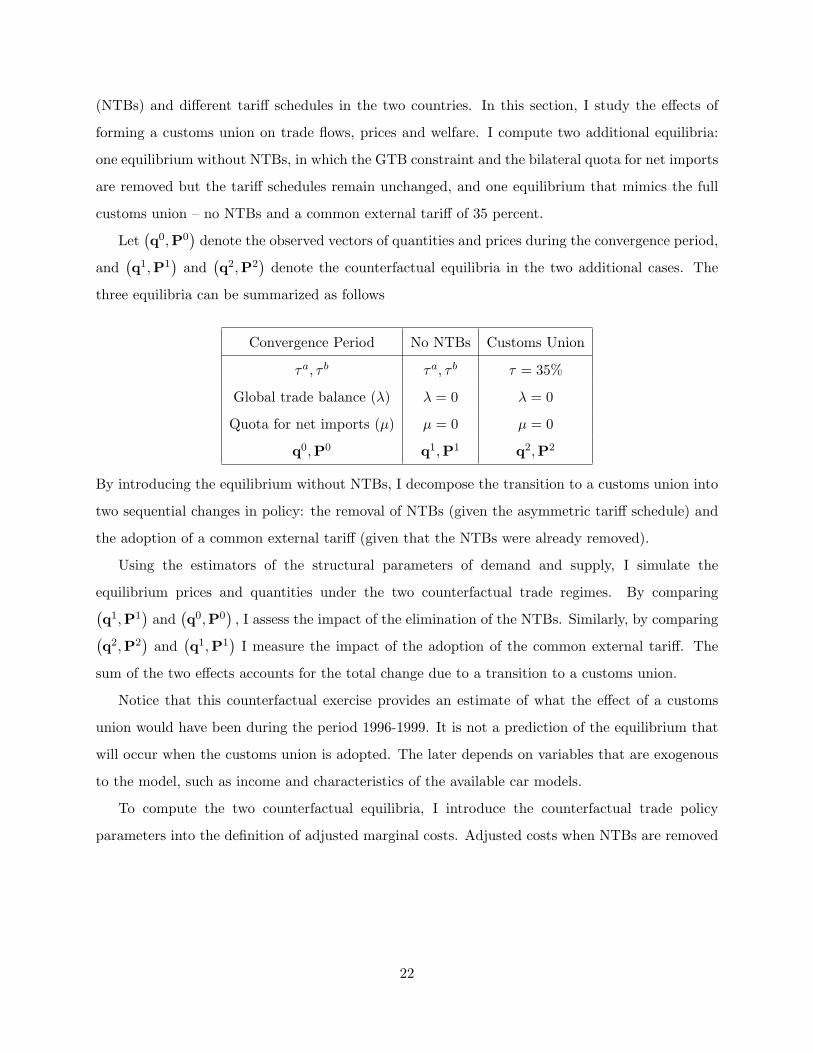
Let(q0,P0

)denote the observed vectors of quantities and prices during the convergence period,

and(q1,P1

)and

(q2,P2

)denote the counterfactual equilibria in the two additional cases. The

three equilibria can be summarized as follows

Convergence Period No NTBs Customs Union

τa, τ b τa, τ b τ = 35%

Global trade balance (λ) λ = 0 λ = 0

Quota for net imports (µ) µ = 0 µ = 0

q0,P0 q1,P1 q2,P2

By introducing the equilibrium without NTBs, I decompose the transition to a customs union into

two sequential changes in policy: the removal of NTBs (given the asymmetric tariff schedule) and

the adoption of a common external tariff (given that the NTBs were already removed).

Using the estimators of the structural parameters of demand and supply, I simulate the

equilibrium prices and quantities under the two counterfactual trade regimes. By comparing(q1,P1

)and

(q0,P0

), I assess the impact of the elimination of the NTBs. Similarly, by comparing(

q2,P2)

and(q1,P1

)I measure the impact of the adoption of the common external tariff. The

sum of the two effects accounts for the total change due to a transition to a customs union.

Notice that this counterfactual exercise provides an estimate of what the effect of a customs

union would have been during the period 1996-1999. It is not a prediction of the equilibrium that

will occur when the customs union is adopted. The later depends on variables that are exogenous

to the model, such as income and characteristics of the available car models.

To compute the two counterfactual equilibria, I introduce the counterfactual trade policy

parameters into the definition of adjusted marginal costs. Adjusted costs when NTBs are removed

22

are given by

c∗ajt =

cjt for j ∈ Aft and j ∈ Bft

cjt(1 + τat ) for j ∈ Wft

(11)

c∗bjt =

cjt for j ∈ A′ft and j ∈ B′

ft

cjt(1 + τ bt ) for j ∈ W ′

ft

Adjusted costs in the full customs union equilibrium are

c∗ajt =

cjt for j ∈ Aft and j ∈ Bft

cjt(1 + τ) for j ∈ Wft

(12)

c∗bjt =

cjt for j ∈ A′ft and j ∈ B′

ft

cjt(1 + τ) for j ∈ W ′ft

Since there are no NTBs in neither of the two computed equilibria, the Lagrange multipliers are

zero.16 Trade between partners is free and the relevant costs are the marginal costs of production.

The adjustment in costs only includes the tariff on imports from the rest of the world. The

elimination of NTBs makes the inter-country strategic component irrelevant and firms set prices

independently in Argentina and Brazil.

The estimator of(q1,P1

)satisfies the system of first order conditions given the estimated

demand function and marginal costs. Let q (P, θ) denote the demand function (with the demand

parameters summarized by the vector θ), ∆ (P, θ) the matrix of cross price derivatives, θ the

estimator of the demand parameters, and c the estimator of the marginal costs of production. The

estimator(q1, P1

)solves17

q(P1, θ) + ∆(P1, θ)(P1 − c∗(c, λ = 0, µ = 0, τa, τ b)

)= 0

q1=q(P1, θ)16The Lagrange multipliers are reduced form parameters. Their estimators are valid only for the particular trade

policy during the convergence period. Hence, the only counterfactual equilibria that can be consistently simulatedare those that involve removing all NTBs. The value of the Lagrange multipliers is known to be zero in these cases.

17Even though the system is non-linear and does not have a closed-form solution, I find that the operator

P1(n+1) = c∗(.)−∆(P1

(n), bθ)−1q(P1

(n), bθ)

works in practice like a contraction mapping and reaches a unique fixed-point in a small number of iterations.

23

Likewise, the estimator of(q2,P2

)is defined by

q(P2, θ) + ∆(P2, θ)(P2 − c∗(c, λ = 0, µ = 0, τa = τ b = 35%)

)= 0

q2=q(P2, θ)

By comparing quantities and prices in the different equilibria I estimate the changes in trade

flows, profits and tariff revenue and I decompose these changes into those caused by the elimination

of NTBs and those caused by the adoption of a uniform tariff.

To measure the change in consumers’ welfare I use the compensating variation, defined as the

negative of the change in income that leaves utility unchanged after a change in prices. In the

comparison of the equilibrium without NTBs and the observed convergence period equilibrium,

such change in income for consumer i at time t and country h, ∆y1,hit , satisfies

maxj

Uhjt

(yh

it + ∆y1,hit , p1,h

jt , θh)

= maxj

Uhjt

(yh

it, p0,hjt , θh

). (13)

This is the change in individual welfare due to the elimination of NTBs. The change due to the

adoption of a common external tariff is given by the additional change in income, ∆y2,hit , that solves

maxj

Uhjt

(yh

it + ∆y1,hit + ∆y2,h

it , p2,hjt , θh

)= max

jUh

jt

(yh

it, p0,hjt , θh

). (14)

To compute the change in aggregate welfare I take a sample of 1,300 and 2,000 individuals for

each time period-region combination in Argentina and Brazil, respectively (only time periods for

Brazil since regional data is not available). I compute the ∆y1,hit and ∆y2,h

it that solve (13) and (14)

given the estimator of utility parameters θ for each sampled individual and calculate the average

change in income across individuals.18 The aggregate change in welfare is the average change in

income multiplied by the market size.

I estimate the variance of the estimated quantities and prices, of the change in the trade flows,

profits and tariff revenue, and of the compensating variation by taking draws of θ from its asymptotic18The change in income for each individual does not have a closed form solution; I take draws of ε for each car

model from a type-I extreme-value distribution and numerically search over different changes in income; each stepinvolves finding the preferred car model.

24

distribution and recomputing all estimators for each sampled value of θ .19,20 The estimators are

not normal because of the non-negativity constraint imposed in the estimation of the Lagrange

multipliers in the cost side.

Results

Table 6 shows the proportional changes in prices of imports and trade volumes due to the

changes in policy. The first two columns show the changes in external imports in Argentina and

Brazil; the total effect is decomposed to capture the effect of the elimination of the NTBs and

the adoption of the common external tariff. Both changes in policies have the expected results.

The elimination of the trade balance constraint results in a sales-weighted average decrease in the

price of external imports of 15 percent in Argentina and 10 percent in Brazil; the number of cars

imported from other countries increases by 78 percent and 117 percent in Argentina and Brazil,

respectively.

The increase in the tariff level due to the adoption of the common external tariff has the opposite

effect. Prices of external imports go up by 12 percent in Argentina and 0.7 percent in Brazil - the

increase is small in Brazil because the counterfactual change in the tariff level is not high. The

number of imported cars decreases by 72 percent in Argentina and 4 percent in Brazil. All these

changes (both due to the elimination of NTBs and to the adoption of the common external tariff)

are significant at the 10 percent level.21

Overall, the effect of the elimination of the NTBs predominates and there is a net increase in

imports from the rest of the world although a customs union is formed. The trade creating effect

of the elimination of the NTBs more than compensates the trade diverting effect of the higher

external tariff. In Argentina the overall effect is relatively small - the average increase in price is 3

percent; the number of imported units increases by 6 percent - and not statistically significant. In

Brazil the effect of the change in the external tariff is very small and the overall change is mostly19Berry, Linton and Pakes (2004) provide a formal proof of the consistency and asymptotic normality of the Berry

(1994) and Berry, Levinsohh and Pakes (1995) estimator of demand.20Notice that for each draw it is also necessary to reestimate the marginal costs and Lagrange multipliers.21I do not compute 95 percent confidence intervals. This computation would involve the estimation of the 2.5 and

9.7 percentiles, which would require a large number of simulated draws as they are further away from the median.Additionally, as can be seen in the 90 percent confidence intervals, the distribution is not symmetric. The longtail on one side adds difficulty to the precise estimation of the limiting percentiles. Note also that this asymmetrymakes it impossible to compare the variance of the estimators to the variance that would arise from a standardnormal distribution. In particular, the 70 percent confidence intervals in the skewed distribution (not shown) aresubstantially smaller than the 70 percent intervals that would result from the hypothetical normal distributions thatyield the 90 percent confidence intervals displayed in Table 6.

25

explained by the positive effect of the elimination of the NTBs.

The last two columns show the changes in bilateral trade flows and prices. As was expected

from the estimation of the Lagrange multipliers, imports from Brazil to Argentina are artificially

high due to the GTB. The cost imposed by the GTB is larger in Brazil and firms have incentives

to switch export credits from Brazil to Argentina; the perceived cost of imports from Brazil to

Argentina is lower than the cost of production. Once this distortion is removed by eliminating the

GTB, the cost of Brazilian cars becomes higher in Argentina and prices of these vehicles go up (7

percent in average). The opposite happens in Brazil, where the price of Argentine vehicles decrease

by 5 percent. Bilateral imports decrease in one direction and increase in the other. The estimates

are relatively large in magnitude (43 and 13 percent respectively) but not precisely estimated and

zero falls within the 90 percent confidence interval. The net effect is an increase in bilateral trade

(not shown in the table).

Bilateral trade increases due to the increase in the external tariff (trade diversion). In Argentina

both changes move in opposite directions with the net effect being negative. Imports from Brazil

are reduced after the counterfactual customs union is adopted. In Brazil, both changes dictate an

increase in bilateral trade.

Table 7 displays the changes in welfare levels after both changes in policy. On average, prices

go down by 659 dollars in Argentina and up by 205 dollars in Brazil and as a result consumers

are better off in the first country and worse off in the second. Argentine consumers gain 393

dollars per vehicle sold whereas their Brazilian peers lose 204 per vehicle. When aggregating the

two countries, consumers are worse off (not shown in table). Revenue increases in both countries

since the counterfactual tariff level is higher and imports are also higher due to the removal of the

NTBs. The aggregate domestic welfare change (compensating variation plus tariff revenue, without

including firms’ profits since they are foreign-owned) are positive in both countries (not shown).

Firm profits decrease by 22 percent in Argentina and increase by 5.7 percent in Brazil; the net

effect is a gain for firms, which can be interpreted as a shift in profits from one country to the

other.22

22The percentage increase in Brazil is smaller than the percentage decrease in Argentina, however, being that Brazilis a larger country, the opposite happens when considering levels.

26

7 Conclusions

After estimating a model of demand and supply for cars in Argentina and Brazil that incorporates

two non-tariff barriers (a quota on bilateral net imports and a trade balance constraint), I predict

the effects of fully including the automobile sector in the Mercosur agreement. The trade reform

involves the removal of NTBs and the adoption of a common external tariff. One of the main

findings is that the effects on prices, trade and welfare are driven by the removal of NTBs rather

than by the convergence to a common external tariff.

The elimination of the NTBs comprises a movement towards free trade that leads to an increase

in external imports (countries from outside the customs union) both in Argentina and Brazil. On

the other hand, the interaction between the trade balance constraint and the ownership structure

of the firms (multinational corporations with subsidiaries in both countries) leads to asymmetric

effects on bilateral trade and welfare for each partner when these restrictions are removed. This

asymmetry is also observed in the total effects of the customs union. In particular, I find that for

most firms, the trade balance constraints create an incentive to export from Brazil to Argentina.

When these particular NTBs are removed, bilateral imports decrease in Argentina and increase in

Brazil, with an overall increase in bilateral trade.

Consumers in Argentina are better off after the customs union, while they are worse off in Brazil.

The opposite is true for profits of Argentine and Brazilian subsidiaries. Tariff revenue increases in

both countries, and in Brazil more than compensates the loss suffered by consumers.

By modeling the behavior of firms in two countries, rather than in one, I am able to capture

an additional strategic component of firm behavior - the interaction across markets. In addition,

from a methodological point of view, the data on two different markets allows me to estimate the

supply parameters (including the shadow cost of the trade policy constraints) by minimum distance

instead of by a perfect fit method, and without the need to make functional form assumptions on

the cost side as is the usual practice in the literature.

References

Berry, S. (1994): “Estimating Discrete Choice Models of Product Differentiation,” RAND Journal

of Economics, Vol. 25, No. 2, 242-262.

27

Berry, S., J. Levinsohn and A. Pakes (1995): “Automobile Prices in Market Equilibrium,”

Econometrica, Vol. 63, No. 4, 841-890.

Berry, S., J. Levinsohn and A. Pakes (1999): “VERs on Automobiles: Evaluating a Trade Policy,”

American Economic Review, Vol. 89, No. 3, 400-430.

Berry, S., O. Linton and A. Pakes (2004): “Limit Theorems for Estimating the Parameters of

Differentiated Product Demand Systems,” Review of Economic Studies, Vol. 71, No. 3, 613-654.

Deaton, A. and J. Muellbauer (1980): Economics and Consumer Behavior, Cambridge, Cambridge

University Press.

Dixit, A. (1988): “Optimal Trade and Industrial Policy for the U.S. Automobile Industry,” in R.

Feenstra, ed., Empirical Methods for Industrial Trade, Cambridge, MA, MIT Press.

Feenstra, R. (1984): “Voluntary Export Restraint in U.S. Autos, 1980-81: Quality, Employment

and Welfare Effects,” in R.E. Baldwin and A. Krueger, eds., The Structure and Evolution of Recent

U.S. Trade Policy, Chicago, University of Chicago Press.

Feenstra, R. (1988): “Quality Change under Trade Restraints in Japanese Autos,” Quarterly

Journal of Economics, Vol. 103, No. 1, 131-146.

Goldberg, P. (1995): “Product Differentiation and Oligopoly in International Markets: the Case of

the U.S. Automobile Industry,” Econometrica, Vol. 63, No. 4, 891-951.

Goldberg, P. and F. Verboven (2001): “The Evolution of Price Dispersion in the European Car

Market,” Review of Economics Studies, Vol. 68, No. 4, 811-848.

Nevo, A. (2000): “Mergers with Differentiated Products: the Case of the Ready-to-eat Cereal

Industry,” RAND Journal of Economics, Vol. 31, No. 3, 395-421.

Nevo, A. (2001): “Measuring Market Power in the Ready-to-eat Cereal Industry,” Econometrica,

Vol. 69, No. 2, 307-342.

Petrin, A. (2002): “Quantifying the Benefits of New Products: The Case of the Minivan,” Journal

of Political Economy, Vol. 110, No. 4, 705-729.

Verboven, F. (1996): “International Price Discrimination in the European Car Market,” RAND

Journal of Economics, Vol 27, No. 2, 240-268.

28

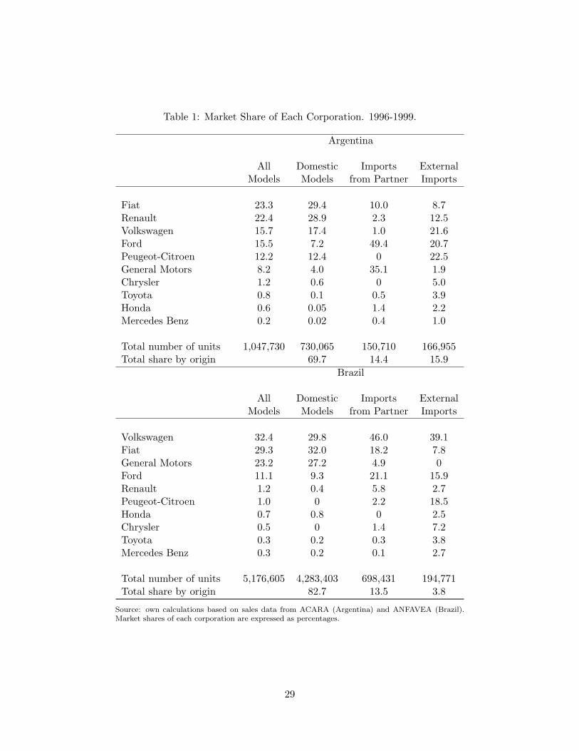
Table 1: Market Share of Each Corporation. 1996-1999.

Argentina

All Domestic Imports ExternalModels Models from Partner Imports

Fiat 23.3 29.4 10.0 8.7Renault 22.4 28.9 2.3 12.5Volkswagen 15.7 17.4 1.0 21.6Ford 15.5 7.2 49.4 20.7Peugeot-Citroen 12.2 12.4 0 22.5General Motors 8.2 4.0 35.1 1.9Chrysler 1.2 0.6 0 5.0Toyota 0.8 0.1 0.5 3.9Honda 0.6 0.05 1.4 2.2Mercedes Benz 0.2 0.02 0.4 1.0

Total number of units 1,047,730 730,065 150,710 166,955Total share by origin 69.7 14.4 15.9

Brazil

All Domestic Imports ExternalModels Models from Partner Imports

Volkswagen 32.4 29.8 46.0 39.1Fiat 29.3 32.0 18.2 7.8General Motors 23.2 27.2 4.9 0Ford 11.1 9.3 21.1 15.9Renault 1.2 0.4 5.8 2.7Peugeot-Citroen 1.0 0 2.2 18.5Honda 0.7 0.8 0 2.5Chrysler 0.5 0 1.4 7.2Toyota 0.3 0.2 0.3 3.8Mercedes Benz 0.3 0.2 0.1 2.7

Total number of units 5,176,605 4,283,403 698,431 194,771Total share by origin 82.7 13.5 3.8

Source: own calculations based on sales data from ACARA (Argentina) and ANFAVEA (Brazil).Market shares of each corporation are expressed as percentages.

29

Table 2: Utility Function Parameters.

Argentina BrazilConstant (−uo) -13.5 -7.7

(27.4) (33.4)Constant*N(0,1) (−u1) 0.9 0.8

(0.6) (0.9)Price (−α0) -0.19*** -0.09***

(0.05) (0.03)Price*1/Income (−α1) -0.17** 0.03***

(0.08) (0.01)Length (βLength,0) 4.2*** 0.4**

(0.3) (0.2)Length*More than 2 children (βLength,1) 1.0 0.4

(0.5) (14.7)Length Square -0.5 0.1

(1.5) (3.0)Horsepower 3.3*** 0.4***

(1.3) (0.1)Hatchback Dummy 0.1 0.4

(0.5) (1.0)Station Wagon Dummy -0.7** -0.6***

(0.3) (0.2)SUV or Minivan Dummy 0.5 0.5

(1.5) (0.5)

Category Dummies Yes Yes

Test of Overidentifying Restrictions 20.84 17.45Critical Value: 23.68

Mean price coefficient -0.25 -0.08(0.11) (0.03)

Standard errors are reported in parenthesis; *** significant at the 1% level; ** significantat the 5% level. The null hypothesis of the test of overidentifying restrictions sustainsthat the orthogonality conditions of the GMM estimator of the demand parameters arestatistically not significantly different from zero.

30

Table 3: Price, Demand Elasticity, Production Cost, and Mark-ups. 1996-1999.

All Domestic Imports from ExternalModels Models Partner Imports

Argentina

Number of Vehicles 1,047,730 730,065 150,710 166,955

Mean Price (thousands) 16.7 15.7 15.1 22.4

Mean Price Elasticity -3.4 -3.3 -3.3 -3.7(0.2) (0.2) (0.2) (0.9)

Mean Production Cost (thousands) 11.3 10.5 11.6 14.7[9, 14] [9, 13] [10, 14] [11, 17]

Mean Percentage Mark-up 50 53 37 48[42, 79] [51, 76] [15, 72] [34, 96]

Brazil

Number of Vehicles 5,176,605 4,283,403 698,431 194,771

Mean Price (thousands) 15.1 14.3 15.9 29.0

Mean Price Elasticity -1.7 -1.5 -1.8 -4.0(0.3) (0.1) (0.2) (0.5)

Mean Production Cost (thousands) 9.7 9.5 9.4 15.3[6, 11] [6, 10] [6, 10] [12, 17]

Mean Percentage Mark-up 60 62 52 39[14, 123] [14, 124] [11, 131] [26, 84]

Prices and production costs are measure in thousands of dollars. The estimators of the production costs andmark-ups are not normally distributed; confidence intervals at the 10% significance level are reported betweensquare brackets. Standard errors are displayed in parenthesis for the mean price elasticities.

31

Table 4: Global Trade Balance Constraint (GTB).

Adjustment in Cost Adjustment in Costof External Imports of Imports from Partner

Argentina Brazil Argentina Brazilλa λb λa − 1.2λb λb − 1.2λa

Chrysler 0.02 0.29** -0.33* 0.27*(0.15) (0.01) [-4.36, -0.02] [0.02, 0.35]

Fiat 0 0.15** -0.19* 0.15*(0.87) (0.03) [-0.36, -1.2] [0.01, 0.30]

Ford 0.50 0.62** -0.25* 0.03(0.43) (0.01) [-0.30, -0.01] [-0.25, 0.24]

General Motors 0.40 0.43** -0.11 -0.05(0.15) (0.00) [-0.25, 0.09] [-0.20, 0.21]

Honda 0 0.37** -0.45* 0.37*(0.98) (0.00) [-0.71, -0.27] [0.22, 0.59]

Mercedes Benz 0 0.15 -0.18 0.15(0.58) (0.24) [-0.61, 0.12] [-0.15, 0.51]

Peugeot-Citroen 0.30 0.43* -0.21 0.07(0.38) (0.10) [-2.00, 0.03] [-0.05, 0.63]

Renault 0 0.48* -0.57* 0.48*(0.99) (0.00) [-0.94, -0.36] [0.30, 0.78]

Toyota 0 0.27** -0.33* 0.27*(0.91) (0.00) [-1.00, -0.11] [0.09, 0.84]

Volkswagen 0 0.14** -0.16* 0.14(0.80) (0.04) [-0.44, -0.01] [0.01, 0.37]

The first two columns display the estimates of the Lagrange Multipliers for the Global TradeBalance Constraint (GTB). They reflect the percentage additional cost on external importsimposed by the GTB. The estimators are constrained to be non-negative. The estimatedprobability that the estimator is equal to zero is displayed in parenthesis. ** indicates differentfrom zero at the 5% significance level (one-sided test) and * at the 10% level.The last two columns display the estimated additional cost that the GTB imposes on bilateralimports, taking into consideration that an imported unit involves a credit for the exportingpartner country. The estimators are not normally distributed; 90% confidence intervals arereported in square brackets. * indicates that the estimator is significant at the 10% level.

32

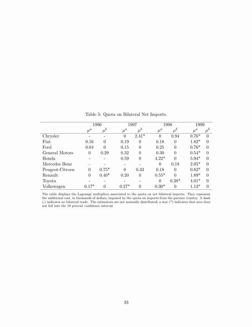
Table 5: Quota on Bilateral Net Imports.

1996 1997 1998 1999µa µb µa µb µa µb µa µb

Chrysler - - 0 2.41* 0 0.94 0.76* 0Fiat 0.16 0 0.19 0 0.18 0 1.82* 0Ford 0.04 0 0.15 0 0.25 0 0.76* 0General Motors 0 0.29 0.32 0 0.30 0 0.54* 0Honda - - 0.59 0 4.22* 0 5.94* 0Mercedes Benz - - - - 0 0.18 2.05* 0Peugeot-Citroen 0 0.75* 0 0.33 0.18 0 0.82* 0Renault 0 0.40* 0.20 0 0.55* 0 1.89* 0Toyota - - - - 0 0.38* 4.01* 0Volkswagen 0.17* 0 0.27* 0 0.30* 0 1.13* 0

The table displays the Lagrange multipliers associated to the quota on net bilateral imports. They representthe additional cost, in thousands of dollars, imposed by the quota on imports from the partner country. A dash(-) indicates no bilateral trade. The estimators are not normally distributed; a star (*) indicates that zero doesnot fall into the 10 percent confidence interval.

33

Table 6: Counterfactual Changes in Prices of Imports and Trade Flows.

External Imports

Argentina Brazil

Elimination of NTBsAverage change in price -15% [-23, -9] -10% [-23, -9]Change in number of units 78% [31, 821] 117% [69, 399]

Adoption of common external tariffAverage change in price 12% [10, 13] 0.7% [0.5, 0.8]Change in number of units -72% [-625, -45] -4% [-10, -2]

Overall customs union effectAverage change in price -3% [-13, 5] -9% [-21, -0.5]Change in number of units 6% [-19, 252] 113% [67, 395]

Imports from Partner

Argentina Brazil

Elimination of NTBsAverage change in price 7% [-21, 8] 5% [28, 2]Change in number of units -43% [-96, 15] 13% [-14, 20]

Adoption of common external tariffAverage change in price -0.12% [-0.55, 0.52] 0.007% [0.006, 0.03]Change in number of units 7% [5, 33] 0.13% [0.10, 0.81]

Overall customs union effectAverage change in price 7% [-21, 8] -5% [-28, -2]Change in number of units -36% [-66, 23] 13% [-14, 21]

The average change in price is weighted by sales. The estimators are not normally distributed; 90%confidence intervals are reported in square brackets.

34

Table 7: Welfare Changes from Adopting a Customs Union.

Argentina BrazilChange in prices (dollars) -659 205

[-2672, -551] [-4248, 323]

Compensating variation 393 -204[-9398, 1386] [-332, 607]

Change in revenue (percentage) 162% 210%[77, 619] [158, 384]

Change in profits (percentage) -22% 5.7%[-26, 14] [-10, 4]

The compensating variation is computed per number of vehicles and reported indollars. The estimators are not normally distributed; 90% confidence intervals arereported in square brackets.

35