NAVAL POSTGRADUATE

SCHOOL

MONTEREY, CALIFORNIA

THESIS

Approved for public release; distribution is unlimited

A COMPARISON OF TIMING METHODS IN ORTHOGO-NAL FREQUENCY DIVISION MULTIPLEXING (OFDM)

SYSTEMS

by

Ersoy OZ

September 2004

Thesis Advisor: Roberto Cristi Co-Advisor: Murali Tummala

THIS PAGE INTENTIONALLY LEFT BLANK

i

REPORT DOCUMENTATION PAGE Form Approved OMB No. 0704-0188 Public reporting burden for this collection of information is estimated to average 1 hour per response, including the time for review-ing instruction, searching existing data sources, gathering and maintaining the data needed, and completing and reviewing the col-lection of information. Send comments regarding this burden estimate or any other aspect of this collection of information, including suggestions for reducing this burden, to Washington headquarters Services, Directorate for Information Operations and Reports, 1215 Jefferson Davis Highway, Suite 1204, Arlington, VA 22202-4302, and to the Office of Management and Budget, Paperwork Reduction Project (0704-0188) Washington DC 20503. 1. AGENCY USE ONLY (Leave blank)

2. REPORT DATE September 2004

3. REPORT TYPE AND DATES COVERED Master’s Thesis

4. TITLE AND SUBTITLE: A Comparison of Timing Methods in Orthogonal Frequency Division Multiplexing (Ofdm) Systems 6. AUTHOR(S) Ersoy OZ

5. FUNDING NUMBERS

7. PERFORMING ORGANIZATION NAME(S) AND ADDRESS(ES) Naval Postgraduate School Monterey, CA 93943-5000

8. PERFORMING ORGANIZATION REPORT NUMBER

9. SPONSORING /MONITORING AGENCY NAME(S) AND ADDRESS(ES)

N/A

10. SPONSORING/MONITORING AGENCY REPORT NUMBER

11. SUPPLEMENTARY NOTES The views expressed in this thesis are those of the author and do not reflect the official policy or position of the Department of Defense or the U.S. Government. 12a. DISTRIBUTION / AVAILABILITY STATEMENT Approved for public release; distribution is unlimited

12b. DISTRIBUTION CODE

13. ABSTRACT (maximum 200 words) Orthogonal frequency division multiplexing (OFDM) is being used by wireless local area network (WLAN)

standards, such as IEEE 802.11a, and wireless metropolitan area network (MAN) standards, such as IEEE 802.16a. OFDM is a very efficient communications scheme for wireless ADHOC networks. However, the wireless environment causes inter-symbol interference (ISI) and inter-carrier interference (ICI). Estimating the starting point of an OFDM symbol must be handled efficiently and effectively to reduce the errors. OFDM must be time synchronized to prevent inter-symbol interference (ISI) and inter-carrier interference (ICI). Many techniques exist to realize timing synchroni-zation in OFDM systems. In this thesis, the need for timing synchronization, the timing errors, and the performance of different techniques under a variety of mobile channel models (indoor and outdoor) are investigated, and simulation performance results for each technique under different channel models are presented.

15. NUMBER OF PAGES

197

14. SUBJECT TERMS. OFDM (Orthogonal Frequency Division Multiplexing), Timing Offset, Coarse Timing Synchronization, Fine Timing Synchronization, Differential Decoding, IFFT (Inverse Fast Fourier Transform), Cyclic Prefix, FFT, MATLAB, Additive White Gaussian Noise (AWGN), Mobile Channels, Convolutional Encoding, Probability of Bit Error. 16. PRICE CODE

17. SECURITY CLASSIFICA-TION OF REPORT

Unclassified

18. SECURITY CLASSIFICA-TION OF THIS PAGE

Unclassified

19. SECURITY CLAS-SIFICATION OF AB-STRACT

Unclassified

20. LIMITATION OF ABSTRACT

UL NSN 7540-01-280-5500 Standard Form 298 (Rev. 2-89) Prescribed by ANSI Std. 239-18

ii

THIS PAGE INTENTIONALLY LEFT BLANK

iii

Approved for public release; distribution is unlimited

A COMPARISON OF TIMING METHODS IN ORTHOGONAL FREQUENCY DIVISION MULTIPLEXING (OFDM) SYSTEMS

Ersoy Oz

First Lieutenant, Turkish Army B.S., Turkish Army Academy, 1999

Submitted in partial fulfillment of the requirements for the degree of

MASTER OF SCIENCE IN ELECTRICAL ENGINEERING

from the

NAVAL POSTGRADUATE SCHOOL September 2004

Author: Ersoy Oz Approved by: Roberto Cristi

Thesis Advisor

Murali Tummala Co-Advisor

John Powers Chairman, Department of Electrical and Computer Engineering

iv

THIS PAGE INTENTIONALLY LEFT BLANK

v

ABSTRACT

Orthogonal frequency division multiplexing (OFDM) is being used by wireless

local area network (WLAN) standards, such as IEEE 802.11a, and wireless metropolitan

area network (MAN) standards, such as IEEE 802.16a. OFDM is a very efficient com-

munications scheme for wireless ADHOC networks. However, the wireless environment

causes inter-symbol interference (ISI) and inter-carrier interference (ICI). Estimating the

starting point of an OFDM symbol must be handled efficiently and effectively to reduce

the errors. OFDM must be time synchronized to prevent inter-symbol interference (ISI)

and inter-carrier interference (ICI). Many techniques exist to realize timing synchroniza-

tion in OFDM systems. In this thesis, the need for timing synchronization, the timing er-

rors, and the performance of different techniques under a variety of mobile channel mod-

els (indoor and outdoor) are investigated, and simulation performance results for each

technique under different channel models are presented.

vi

THIS PAGE INTENTIONALLY LEFT BLANK

vii

TABLE OF CONTENTS

I. INTRODUCTION........................................................................................................1 A. OBJECTIVE ....................................................................................................1 B. RELATED RESEARCH.................................................................................2 C. ORGANIZATION OF THE THESIS............................................................2

II. OFDM BASICS............................................................................................................5 A. INTRODUCTION TO OFDM........................................................................5 B. FUNDAMENTALS OF OFDM......................................................................6

1. Wireless Propagation...........................................................................6 a. Power Delay Profile and RMS Delay Spread ..........................7 b. Coherence Bandwidth...............................................................8 c. Doppler Spread and Coherence Time ....................................10

2. Orthogonality .....................................................................................11 3. Cyclic Prefix, Inter-Symbol Interference, and Inter-Carrier

Interference ........................................................................................13 4. The Description of the OFDM System Used in This Thesis...........15 5. IEEE 802.11a......................................................................................18 6. IEEE 802.16a......................................................................................21

C. SUMMARY ....................................................................................................23

III. TIMING SYNCHRONIZATION AND INTRODUCTION OF ALGORITHMS .........................................................................................................25 A. THE NEED FOR TIMING SYNCRONIZATION AND TIMING

ERRORS.........................................................................................................25 B. COARSE TIMING ........................................................................................28 C. FINE TIMING ...............................................................................................33

1. Schmidl and Cox Method..................................................................33 2. Minn and Bhargava Method.............................................................36 3. Park et al. Method..............................................................................38 4. Wang et al. Method............................................................................40 5. Proposed Method 1 (a Modification of the Park et al. Method)....43 6. Proposed Method 2 ............................................................................45

D. SUMMARY ....................................................................................................49

IV. OFDM SYSTEM SIMULATIONS IN MATLAB ..................................................51 A. SELECTING SYSTEM PARAMETERS....................................................51 B. SIMULATION METHODOLOGY .............................................................52

1. Code Check (Ideal Channel) .............................................................54 2. OFDM Performance in AWGN Channel ........................................56 3. Performance under Mobile Channels ..............................................58

a. Mobile Indoor Channels.........................................................58 b. Mobile Outdoor Channels ......................................................59 c. Channel Simulations ..............................................................60

viii

C. PERFORMANCE OF TIMING METHODS .............................................63 1. Schmidl and Cox Method..................................................................64 2. Minn and Bhargava Method.............................................................68 3. Park et al. Method..............................................................................73 4. Wang et al. Method............................................................................77 5. Proposed Method 1 (a Modification of the Park et al. Method)....81 6. Proposed Method 2 ............................................................................85 7. Comparison of the Timing Methods ................................................90

D. SUMMARY ....................................................................................................93

V. CONCLUSION ..........................................................................................................95 A. SUMMARY OF THE WORK DONE..........................................................95 B. SIGNIFICANT RESULTS AND CONCLUSIONS....................................95 C. SUGGESTIONS FOR FUTURE STUDIES................................................96

APPENDIX A. MATLAB CODE.........................................................................................97

LIST OF REFERENCES....................................................................................................169

INITIAL DISTRIBUTION LIST .......................................................................................175

ix

LIST OF FIGURES

Figure 1. A Multi-path Illustration for Outdoor Channel Environment............................7 Figure 2. Illustration of (a) Flat Fading Channel (b) Frequency Selective Fading

Channel ..............................................................................................................9 Figure 3. A Single-carrier Illustration ...............................................................................9 Figure 4. OFDM Has Longer Symbol Period and Multiple Symbols are Transmitted

Simultaneously over Multiple Sub-carriers .....................................................10 Figure 5. Orthogonality of Sub-carriers (After Ref. 32.) ................................................12 Figure 6. Illustration of Loss of Orthogonality and Inter-carrier Interference (ICI).......13 Figure 7. Illustration of ISI (After Ref. 31.)....................................................................14 Figure 8. Illustration of the Relationship between CIR and CP (After Ref. 32.) ............15 Figure 9. The Block Diagram of Base-band OFDM Model Used in This Thesis: (a)

Transmitter and (b) Receiver ...........................................................................16 Figure 10. QPSK Constellation (From Ref. 2.) .................................................................17 Figure 11. Adding CP to the OFDM Symbol....................................................................18 Figure 12. IEEE 802.11a Preamble (After Ref. 2.) ...........................................................21 Figure 13. Illustration of ISI and ICI in OFDM Systems..................................................26 Figure 14. The Effect of ISI and ICI due to Early Timing under Mobile Indoor

Channel 1 .........................................................................................................27 Figure 15. The Effect of ISI and ICI due to Late Timing with an Offset of 100 ns

under Mobile Indoor Channel 1.......................................................................28 Figure 16. Detection by Energy over a Window...............................................................30 Figure 17. Illustration of Double Sliding Window Detection Algorithm (After Ref.

1.) .....................................................................................................................31 Figure 18. Detection by Double Sliding Window Technique in AWGN Channel

with 15 dBb oE N = .........................................................................................32 Figure 19. Signal Detection by Proposed Method 2 .........................................................33 Figure 20. Timing Metric for Schmidl and Cox Method under Ideal Conditions with

No Channel Effect and No Noise.....................................................................35 Figure 21. Timing Metric for Minn and Bhargava Method [4] under Ideal Conditions

with No Channel Effect and No Noise ............................................................38 Figure 22. Timing Metric for Park et al. Method under Ideal Conditions with No

Channel Effect and No Noise ..........................................................................40 Figure 23. Metrics: (a) 1( )m n and (b) 2 ( )m n ....................................................................41 Figure 24. Coarse Timing Metric ( )4M n .........................................................................42 Figure 25. Illustration of How the Algorithm for Proposed Method 1 Works..................44 Figure 26. Timing Metric for Proposed Method 1 under Ideal Conditions with No

Channel Effect and No Noise ..........................................................................45 Figure 27. Timing Metric for Proposed Method 2 for Fine Timing (first algorithm).......47 Figure 28. Timing Metric for Proposed Method 2 for Coarse Timing (second

algorithm).........................................................................................................49

x

Figure 29. Matlab Simulations Scheme ............................................................................53 Figure 30. (a) Transmitted and (b) Received QPSK Constellations for Ideal Channel

Conditions ........................................................................................................55 Figure 31. (a) Transmitted and (b) Received 8-PSK Constellations for Ideal Channel

Conditions ........................................................................................................55 Figure 32. Received QPSK Constellation for the AWGN Channel with

10 dBb oE N = and 2000 Symbols .................................................................56 Figure 33. BER Plots for QPSK Simulation in AWGN Channel (a) From Ref. 13, (b)

Simulated .........................................................................................................57 Figure 34. Magnitude Variation in AWGN Channel with 10 dBb oE N = , (a)

Transmitted Packet, (b) Received Packet ........................................................57 Figure 35. Modeling of Mobile Indoor Channels Using FIR Filters and Delay

Elements D (from Ref. 13)...............................................................................58 Figure 36. Effects of Mobile Channels on QPSK Signal Constellation (Before

Differential Decoding), (a) Mobile Indoor Channel 1 (From Ref. 13.), (b) Mobile Indoor Channel 2 (From Ref. 13.), (c) Mobile Outdoor Channel 4, (d) Mobile Outdoor Channel 3.........................................................................61

Figure 37. Effect of Mobile Channels on the Magnitude Plot of a Received OFDM Packet with 12,000 symbols, (a) Mobile Indoor Channel 1, (b) Mobile Indoor Channel 2, (c) Mobile Outdoor Channel 3, (d) Mobile Outdoor Channel 4 .........................................................................................................62

Figure 38. BER versus b oE N Plots for QPSK Simulation for Different Channels (From Ref. 13.) ................................................................................................63

Figure 39. Schmidl and Cox Method under: (a) AWGN Channel, (b) Mobile Channel 1, (c) Mobile Channel 2, (d) Mobile Channel 3, and (e) Mobile Channel 4....65

Figure 40. Peak Magnitude Degradation of the Schmidl and Cox Method ......................66 Figure 41. Fine Timing Distribution of Schmidl and Cox Method for: (a) Mobile

Channel 1, (b) Mobile Channel 2, (c) Mobile Channel 3, and (d) Mobile Channel 4 with 10 dBb oE N = and 300 Runs................................................67

Figure 42. Minn and Bhargava Method for: (a) AWGN Channel, (b) Mobile Channel 1, (c) Mobile Channel 2, (d) Mobile Channel 3, and (e) Mobile Channel 4....69

Figure 43. Central Peak as Shown in [4]...........................................................................70 Figure 44. Peak Magnitude Degradation of the Minn and Bhargava Method ..................70 Figure 45. Fine Timing Distribution for Minn and Bhargava Method for: (a) Mobile

Channel 1, (b) Mobile Channel 2, (c) Mobile Channel 3, and (d) Mobile Channel 4 with 10 dBb oE N = and 300 Runs................................................72

Figure 46. Park et al. Method for: (a) AWGN Channel, (b) Mobile Channel 1, (c) Mobile Channel 2, (d) Mobile Channel 3, and (e) Mobile Channel 4 .............74

Figure 47. Peak Magnitude Degradation of the Park et al. Method.................................75 Figure 48. Fine Timing Distribution of Park et al. Method for: (a) Mobile Channel 1,

(b) Mobile Channel 2, (c) Mobile Channel 3, and (d) Mobile Channel 4 with 10 dBb oE N = and 300 Runs .................................................................76

xi

Figure 49. Wang et al. Method for Coarse Timing for: (a) AWGN Channel, (b) Mobile Channel 1, (c) Mobile Channel 2, (d) Mobile Channel 3, and (e) Mobile Channel 4............................................................................................78

Figure 50. Peak Magnitude Degradation of the Wang et al. Method for Coarse Timing..............................................................................................................79

Figure 51. Fine Timing Distribution of Wang et al. Method for: (a) Mobile Channel 1, (b) Mobile Channel 2, (c) Mobile Channel 3, and (d) Mobile Channel 4 with 10 dBb oE N = and 300 Runs .................................................................80

Figure 52. Proposed Method 1 for: (a) AWGN Channel, (b) Mobile Channel 1, (c) Mobile Channel 2, (d) Mobile Channel 3, and (e) Mobile Channel 4 .............82

Figure 53. Peak Magnitude Degradation of the Proposed Method 1 ................................83 Figure 54. Fine Timing Distribution of Proposed Method 1 for: (a) Mobile Channel

1, (b) Mobile Channel 2, (c) Mobile Channel 3, and (d) Mobile Channel 4 with 10 dBb oE N = and 300 Runs .................................................................84

Figure 55. Proposed Method with 16-sample PN Sequence for: (a) Mobile Channel 1, (b) Mobile Channel 2, (c) Mobile Channel 3, and (d) Under Mobile Channel 4 .........................................................................................................86

Figure 56. Fine Timing Distribution of Proposed Method 2 for: (a) Mobile Channel 1, (b) Mobile Channel 2, (c) Mobile Channel 3, and (d) Mobile Channel 4 with 10 dBb oE N = 600 Runs........................................................................87

Figure 57. Peak Magnitude Degradation of the Proposed Method 2 with 16-sample PN Sequence ....................................................................................................88

Figure 58. Proposed Method 2 with 8-sample PN Sequence: (a) Peak Magnitude Degradation, (b) Fine Timing Distribution for Mobile Channel 2, and (c) Timing Metric for Mobile Channel 2...............................................................89

xii

THIS PAGE INTENTIONALLY LEFT BLANK

xiii

LIST OF TABLES

Table 1. OFDM Timing Related Parameters for IEEE 802.11a Standard (From Ref. 2.) .....................................................................................................................19

Table 2. OFDM Rate Dependent Parameters for IEEE 802.11a Standard (From Ref. 2.) .............................................................................................................20

Table 3. Major Parameters of OFDM PHY for IEEE 802.11a Standard (From Ref. 2.) .....................................................................................................................20

Table 4. OFDM Symbol Parameters for IEEE 802.16a (From Ref. 6.).........................22 Table 5. Channelization Parameters for Licensed Bands for IEEE 802.16a;

f∆ denotes the frequency spacing, gT denotes the length of the CP, and WCS stands for wireless communication service (From Ref. 6.)....................22

Table 6. PN Sequence for Training Symbol for the Method in [8] ...............................34 Table 7. PN Sequence to Obtain the Training Symbol in [4] ........................................36 Table 8. PN Sequence to Obtain the Training Sequence 4S .......................................46 Table 9. The Order in Which the Simulations are Executed .........................................54 Table 10. Code Check Simulation Parameters for QPSK and 8-PSK .............................55 Table 11. FIR Filter Coefficients for Indoor Channels....................................................59 Table 12. Mobile Outdoor Channel 3 Parameters with 200 Hzdf = .............................59 Table 13. Mobile Outdoor Channel 4 Parameters with 200 Hzdf = .............................60 Table 14. Mobile Channel Simulation Parameters ..........................................................60 Table 15. Simulation Parameters for Channel Effects with Different AWGN Values....64 Table 16. Performance Evaluation of Timing Methods...................................................90 Table 17. Fine Timing Offset in Samples (* indicates the results for 16-point PN

sequence)..........................................................................................................91

xiv

THIS PAGE INTENTIONALLY LEFT BLANK

xv

LIST OF ACRONYMS

ADSL Asymmetric Digital Subscriber Line AWGN Additive White Gaussian Noise BER Bit Error Rate BWA Broadband Wireless Access CIR Channel Impulse Response CP Cyclic Prefix TACOMS Tactical Area Communications Systems DAB Digital Audio Broadcasting dB Decibel DFT Discrete Fourier Transform DVB Digital Video Broadcasting FCC Federal Communications Commission FEC Forward Error Correction FDM Frequency Division Multiplexing HIPERLAN High Performance Local Area Network ICI Inter Carrier Interference IDFT Inverse Discrete Fourier Transform IEEE Institute of Electrical and Electronics Engineers IFFT Inverse Fast Fourier Transform ISI Inter Symbol Interference MAC Medium Access Control MAN Metropolitan Area Network OFDM Orthogonal Frequency Division Multiplexing PN Pseudo Noise PSK Phase Shift Keying QAM Quadrature Amplitude Modulation QPSK Quadrature PSK RF Radio Frequency RS Reed-Soloman WLAN Wireless Local Area Network 4G Fourth Generation

xvi

THIS PAGE INTENTIONALLY LEFT BLANK

xvii

ACKNOWLEDGMENTS

First of all, I want to thank my family for their endless support. I also would like

to thank my thesis advisors Prof. Roberto Cristi and Prof. Murali Tummala for their sup-

port and help in answering my questions.

Finally, I want to thank my country for giving me the opportunity to obtain educa-

tion at the Naval Postgraduate School.

xviii

THIS PAGE INTENTIONALLY LEFT BLANK

xix

EXECUTIVE SUMMARY

The communication requirements for modern warfare change with technological

developments. Communications and information warfare directly affect the decision

making process in a dynamic warfare environment. More information is required to be

transmitted at higher speeds. The military, facing these challenges in information warfare

and communications, also requires solutions to make high data rate transmission to, from,

and within the battlefield possible. The military is exploring wireless ad hoc networks as

a solution to this problem at the tactical level, such as TACOMS of the Turkish Land

Forces [41], and orthogonal frequency division multiplexing (OFDM) is a useful and re-

liable technique that has the potential to provide high data rates under challenging trans-

mission conditions for ad hoc networks.

OFDM is being successfully used in numerous applications. It was chosen for the

IEEE 802.11a wireless local area network (WLAN) standard, the IEEE 802.16a fixed

broadband metropolitan area network (MAN) standard, and it is being considered for the

fourth-generation mobile communication systems. Studies to introduce mobility to

802.16 systems are in progress under the name of IEEE 802.16e, mobile wireless broad-

band metropolitan area networks. Despite its many attractive features, OFDM has some

principal drawbacks. Sensitivity to inter-symbol interference (ISI) and inter-carrier inter-

ference (ICI) are among the drawbacks. The solution to these drawbacks is fine timing

synchronization.

This thesis investigates the performance of different timing synchronization

methods for OFDM-based systems to determine the effects of different channel condi-

tions for ADHOC networks on these methods. The fundamentals of an OFDM system

and the distortions caused by wireless propagation are presented, and the advantages of

OFDM in such an environment, the basic characteristics of OFDM, such as the inverse

Fourier transform and the cyclic prefix are discussed. The need for timing synchroniza-

tion and the effects of timing errors, inter-symbol interference (ISI), and inter-carrier in-

xx

terference (ICI) are examined, and the distortion caused by ISI and ICI are demonstrated

through bit error rate (BER) performance plots.

We conducted Matlab simulations of an OFDM communication system for the

following channels: ideal, additive white Gaussian noise (AWGN) channel, mobile in-

door, and mobile outdoor channels. The mobile channels used in this thesis are character-

ized by multi-path, delays and losses associated with the multi-path and Doppler fre-

quency shift effects in AWGN. The timing methods of interest were introduced. The ef-

fects of each channel on the timing synchronization methods were studied and simulated.

The results were presented in terms of fine timing distribution plots, performance plots,

and peak degradation plots for all the channel models.

It was observed that, in general, the performance of the timing methods degraded

under the multi-path. It was shown that the fine timing distribution for indoor channel

models used in this thesis, which have as many as 18 paths, span 2 to 8 samples whereas

the fine timing distribution for outdoor channel models used in this thesis, which have 6

paths, span 2 to 4 samples. Multi-path also causes the peak of the timing metric to fall

below the normalized value of 0.5 since it reduces the correlation values on which the

timing algorithms are based.

Another observation is that the larger delays do not affect the timing process. The

reason is that most of the timing methods are based on the energy of the training symbol,

and the larger delays do not interfere with the first symbol to reach the receiver.

The results enabled us to make a comparison between cross-correlation-based

methods and auto-correlation-based methods. In general the cross-correlation based

methods showed a reliable performance for both indoor and outdoor channels.

The effects of mobility were also studied. The mobility is represented by includ-

ing the Doppler frequency shift and multi-path effects. The simulations suggested that a

Doppler shift up to 15 Hz in indoor channels has virtually no effect on the performance of

the timing methods. As for the outdoor channels, it had no adverse effects.

1

I. INTRODUCTION

Orthogonal frequency division multiplexing (OFDM) was chosen as the commu-

nications technique by many applications and standards, such as IEEE 802.11a [2],

802.16a [6], 802.16e [26], European digital audio broadcasting (DAB), digital video

broadcasting (DVB) systems [24, 25], and HIPERLAN/2 [23]. The military is also seek-

ing wireless solutions for communications at the tactical level. OFDM, with its potential

to provide high data rates under challenging transmission conditions, could be the solu-

tion.

The OFDM-based IEEE 802.11a standard can support data rates up to 54 Mbps.

The newly approved OFDM-based wireless metropolitan area network (MAN) standard

IEEE 802.16a is expected to have a range up to 30 miles and the ability to transfer data,

voice and video at data rates of up to 70 Mbps [40]. Another study, namely IEEE

802.16e, to bring mobility to metropolitan area networks (MANs) is in progress [26].

Another area where intense research is in progress is fourth generation (4G) mo-

bile wireless technologies for which the main focus is spectral efficiency. OFDM and

OFDM-based multiple access systems are among the most promising techniques in terms

of spectral efficiency. Moreover, they are being considered for the 4G mobile communi-

cations systems [3]. At the basis of this success is the fact that OFDM effectively deals

with the delay spread at high data rates. Therefore, OFDM’s performance under multi-

path, mobile and fading environments as well as other related issues, such as synchroni-

zation and implementation, are the topics of many current studies.

A. OBJECTIVE OFDM is a very effective communication scheme to overcome delay spread and

channel distortion. However, it does require an effective and tolerably precise timing

synchronization process. In order to recover the data at the receiver, there are many tech-

niques for timing synchronization. The main objective of this thesis was to investigate

and to compare the performance of various timing methods for multi-path, time-varying

channels with indoor and outdoor characteristics as well as with a Doppler shift to repre-

sent the mobility of the channel.

2

B. RELATED RESEARCH OFDM has been the subject of many studies. The number of studies increased

since OFDM’s approval in wireless local area network (WLAN) standards like IEEE

802.11a, HIPERLAN/2 as well as in wired applications, such as the asymmetric digital

subscriber line (ADSL). The trend seems to continue because IEEE 802.16a, a standard

for fixed broadband wireless access (BWA) systems, was approved in 2003. Proposals to

introduce BWA with mobility to reach speeds up to 70 mph are underway.

One of the very first studies on synchronization, which is cited by many authors,

is that of Schmidl and Cox [8]. They proposed that timing synchronization could be

achieved via a pseudo-noise (PN) sequence and correlation. Another early study was

conducted by Sandell, van de Beek, and Borjesson [37]. This study proposed a cyclic pre-

fix (CP) based synchronization scheme.

In later years, researchers made standard-oriented studies on the subject of timing

synchronization. Among these are the study by Abdul Aziz, Nix, and Fletcher [38] on

synchronization in IEEE 802.11a and HIPERLAN/2 and the study of Wang, Faulkner,

Singh, and Tolochko [9], which is based on IEEE 802.11a preamble defined in the stan-

dard. Other studies include the study of Ryu and Han [16] about a timing phase estimator,

the study of A Fort, J. W. Weijers, V. Derudder, W. Eberle, and A. Bourdoux [39] on

comparison of auto-correlation and cross-correlation-based timing methods, the study of

Park, Cheon, Kang and Hong [5] and the study of Minn and Bhargava [4].

Heiskala and Terry give detailed information about coarse timing synchronization

as well as general information about fine timing synchronization [1]. References [21] and

[28] analyze and categorize the studies on timing synchronization.

C. ORGANIZATION OF THE THESIS Chapter II begins with an introduction to OFDM and proceeds to present the

characteristics of a wireless channel and the related distortions. The operation of an

OFDM system model is presented, and IEEE 802.11a and IEEE 802.16a standards are

also introduced briefly. Chapter III discusses the timing synchronization and the timing

errors explaining the impairments caused by timing errors. The timing algorithms of in-

3

terest are introduced in this chapter as well. There are six methods, two of which are pro-

posed in this work.

Chapter IV explains the simulation methodology, the parameters and the channels

used in the simulation. The timing methods are implemented under various channel con-

ditions. This chapter also presents the performance results of the simulations. Chapter V

provides a summary of the thesis and the conclusions and suggestions for future work.

The Matlab code used in this work is included in Appendix A.

4

THIS PAGE INTENTIONALLY LEFT BLANK

5

II. OFDM BASICS

The dramatic growth of voice, data, and video communications over the Internet

fueled a demand for high data rates. Numerous techniques exist in order to meet the in-

creasing demand. OFDM is at the center of these efforts due to its attractive features. In

this chapter, we present the advantages of OFDM, wireless channel characteristics, a sys-

tem description, and two OFDM-based standards.

A. INTRODUCTION TO OFDM The principle of OFDM is that it takes a data stream, and after multiplexing, sends

the data over a range of sub-carriers, thus transmitting the data simultaneously over a

number of different carriers. Each sub-carrier carries a portion of the data. This helps

OFDM reach higher data rates without being affected by the channel distortions. The sub-

carriers are orthogonal to each other. This allows the sub-carriers to overlap in frequency

with the adjacent carriers without causing interference. Another benefit of orthogonality

is high spectral efficiency. Besides being better suited to overcome frequency selective

fading and multi-path effects, OFDM also has implementation advantages, such as avoid-

ing ISI and ICI, over other multi-carrier communication schemes.

The idea of OFDM is not new. It was first studied in the 1950s and 1960s. Chang

obtained a patent for OFDM in 1966 [22]. The implementation then consisted of as many

oscillators in the transmitter and matched filters in the receiver as the number of sub-

carriers. This made the implementation of OFDM very complex and expensive. However,

in 1971 Weinstein and Ebert showed that OFDM could be realized by the inverse discrete

Fourier transform (IDFT) and discrete Fourier transform (DFT) operations [18]. This in-

novation, making the oscillators and the filters redundant, was enough to attract the atten-

tion of many researchers.

OFDM was chosen as the standard communication technique by many wired and

wireless applications today. Among them are Asymmetric Digital Subscriber Line

(ADSL), Digital Audio Broadcasting (DAB) [24], and Digital Video Broadcasting (DVB)

[25]. OFDM is used in the WLAN standards HIPERLAN/2 [23] and IEEE 802.11a [2]. It

6

was also accepted as the communication technique in the so-called “last mile” access

MAN standards IEEE 802.16a [6] in the USA and HIPERMAN [20] in Europe.

The introduction of the IEEE 802.16 standard, surpassing the so-called 3-G wire-

less networks in terms of data transmission capability, has impacted the wireless digital

communications world. The efforts to develop IEEE 802.16e, an amendment to IEEE

802.16a [23], that will enable mobile wireless services and Internet access for speeds up

to 75 mph, is in progress. OFDM will remarkably affect the future of digital communica-

tions, wireless Internet access, and wireless ADHOC networks.

B. FUNDAMENTALS OF OFDM In this section, we present the challenges in a wireless environment and the most

prominent characteristics of OFDM, which make it attractive in overcoming these chal-

lenges.

1. Wireless Propagation In order to better understand the advantages that OFDM provides, we first discuss

the environmental conditions affecting the communication channel. In general, this is

more complex than a free space environment due to obstacles, trees, moving objects, and

furniture that can reflect the radio waves. As a consequence, wireless channels are char-

acterized by multi-path, which lead to small-scale fading. An illustration of an outdoor

multi-path environment is shown in Figure 1.

Small-scale fading is used to describe sudden changes in amplitudes, phases, or

multi-path delays over a short time or over a short travel distance. In the presence of ob-

stacles and scatterers, which create a dynamically changing environment, the signal en-

ergy is dissipated in amplitude, time and phase. Thus, every path does not arrive at the

receiver at the same time and with the same amplitude and phase. This causes small-scale

fading as well as distortion. When there is multi-path, large-scale path loss affects may be

ignored [7].

7

B ST x

R xL O S

B ST x

R xL O S

Figure 1. A Multi-path Illustration for Outdoor Channel Environment

a. Power Delay Profile and RMS Delay Spread The power delay profile can be obtained by transmitting an impulse over

the channel and is defined as the squared absolute value of the channel impulse response

(CIR) [29] as follows:

1

2

0( ) ( )

N

k kk

P t a tδ τ−

=

= −∑ (2.1)

where k is the path index, ka is the path gain, kτ is the path delay, and N is the number

of paths.

The power delay profile is important to obtain multi-path channel parame-

ters, such as mean excess delay (τ ) and root-mean-square (rms) delay spread ( τσ ).

These parameters are used to qualify the dispersive properties of multi-path channels.

The mean excess delay and the rms delay spread are defined in [7] to be

2

2

( )

( )

k k k kk k

k kk k

a P

a P

τ τ ττ

τ= =∑ ∑∑ ∑

(2.2)

2 2( )τσ τ τ= − (2.3)

where

2 2 2

22

( )

( )

k k k kk k

k kk k

a P

a P

τ τ ττ

τ= =∑ ∑∑ ∑

. (2.4)

8

The time delay measurements are computed relative to the first arriving

path at the receiver at 0 0τ = . The values for rms delay spread may change from environ-

ment to environment. In a wireless channel, the scattered and reflected paths may arrive

at the receiver at different times.

b. Coherence Bandwidth Coherence bandwidth is used to describe the channel bandwidth that is not

affected by the random phases, delays and fading. In other words, coherence bandwidth

can be used to define the channel that is enjoying flat fading as opposed to frequency se-

lective fading. In [30], when the frequency correlation function is above 0.5, the coher-

ence bandwidth, CW , is defined as

15CW

τσ≈ . (2.5)

If the bandwidth of the signal, SW , is smaller than coherence bandwidth of

the channel, the signal will undergo flat fading, i.e., all frequencies have the same fading.

In the opposite case, when S CW W> , the signal will undergo frequency selective fading.

This relationship is directly related to the data rate of the signal. Thus the signal will un-

dergo flat fading when the symbol period sT is greater that the delay time DT . It turns out

that the flat fading is a more desirable channel condition. Figure 2 presents a simple rep-

resentation of flat fading and frequency selective fading. The result of frequency selective

fading is ISI, which adversely affects the bit error rate (BER) of the system. The effects

of ISI are discussed later in this chapter, where we show how OFDM can be designed to

mitigate its effects.

9

(a) (b)

Figure 2. Illustration of (a) Flat Fading Channel (b) Frequency Selective Fading Channel

OFDM uses orthogonal sub-carriers to transmit the signal. Each carrier

transmits a portion of the data at the same time. Although the overall data rate remains

the same, the data rate for each sub-carrier decreases proportional to the inverse of the

number of the sub-carriers, thereby causing the bandwidth (BW) of each sub-carrier to

decrease by the same rate. This helps the channel become a flat fading channel. Figure 3

and Figure 4 illustrate the difference between a single-carrier communication scheme and

an OFDM scheme. For example, let the data rate be 10 bpsR = and the numbered sym-

bols be QPSK modulated. In this case, the period of the OFDM symbol is 5 sT , which is 5

times the single-carrier case. For the data rate, R , each sub-carrier has a narrower band-

width ( )5R and is subject to flat fading. This is also a good example of how OFDM can

reach higher data rates in multi-path channels.

Figure 3. A Single-carrier Illustration

10

Figure 4. OFDM Has Longer Symbol Period and Multiple Symbols are Transmitted

Simultaneously over Multiple Sub-carriers

c. Doppler Spread and Coherence Time The time-varying nature of the channel is characterized by the Doppler

spread and the coherence time. Coherence time is a measure of time duration over which

the channel is slow fading. In other words, the channel impulse response (CIR) is time

invariant over this period. Coherence time can be measured via the time correlation of the

channel, and it is the reciprocal of Doppler spread as shown below [7]

max

1CT

f≈ . (2.6)

where the maximum Doppler spread maxf is given by

maxcos 1

cos = , vfθ

ν θλ λ=

= (2.7)

where λ , ν and θ are the wavelength, the velocity, and the spatial angle between the

direction of the motion of the mobile receiver and the direction of arrival of the signal,

respectively. However, if CT is defined as the time over which the time correlation func-

tion takes values above 0.5, then it is defined as [7]

max

916CT

fπ= . (2.8)

According to the amount of the Doppler shift, we classify the channel as

fast fading or slow fading. In a fast-fading channel, the CIR changes within a symbol.

11

This causes distortion in the signal, and the receiver may not recover it. In this case, the

coherence time is smaller than the symbol time. Then, the signal suffers fast fading if

S CT T> . (2.9)

When the channel is slow fading, the CIR changes slower than the signal

in the sense that the CIR does not change within a symbol duration. Then, the signal un-

dergoes slow fading if

S CT T<< . (2.10) 2. Orthogonality

In OFDM, the sub-carriers have overlapping spectra. In order for the receiver to

separate them without ICI, these sub-carriers need to be orthogonal, hence the name or-

thogonal frequency division multiplex (OFDM). Orthogonality can be shown by using

orthogonal waveforms as follows [33]:

*

0

( ) ( ) ( )sT

k lt t dt k lψ ψ δ= −∫ . (2.11)

Normally, frequency division multiplexing (FDM) systems do not have this

property. Each carrier is separated with a guard band to avoid ICI at the cost of low spec-

tral efficiency, which is, besides presenting implementation difficulties, another draw-

back of FDM. OFDM, due to the orthogonality of overlapped sub-carriers, is a bandwidth

efficient communication scheme. In [33], a generic set of orthogonal waveforms is given

as follows:

[ ]1 0,

( )0 otherwise

kj ts

sk

e t TTt

ω

ψ ∈=

(2.12)

where sT denotes symbol period and

02 ; 0,1,..., 1k

s

k k NTπω ω= + = − , (2.13)

and the sub-carrier frequency

2

kkf

ωπ

= . (2.14)

12

Although the sub-channels overlap in frequency, they can be separated from one

another by orthogonality. Figure 5 illustrates the orthogonality of carriers. It can be seen

from Figure 5 that at the center frequency of any sub-carrier, all other carriers have a null

point.

01f

1( )S f

Null

Samplingpoint

2 ( )S f 3( )S f

2f 3ff0

1f

1( )S f

Null

Samplingpoint

2 ( )S f 3( )S f

2f 3ff

Figure 5. Orthogonality of Sub-carriers (After Ref. 32.)

Figure 6 illustrates the loss of orthogonality between two carriers. The solid col-

ored area shows where the ICI occurs (see also Figure 5). The reasons for the loss of or-

thogonality are frequency errors, timing errors and sampling rate offset. For example, or-

thogonality can be lost when the center frequencies of the carriers are shifted. This shift

causes the adjacent carrier’s first null to move away from the center of the adjacent carri-

ers’ spectrum. When the received signal is sampled, the samples would also include

components from the adjacent carriers since they would not have nulls at the sampling

point.

13

Figure 6. Illustration of Loss of Orthogonality and Inter-carrier Interference (ICI)

3. Cyclic Prefix, Inter-Symbol Interference, and Inter-Carrier Interfer-ence

The wireless channel, with multi-path, is a time-dispersive channel by its nature.

Sending the signal through this channel causes inter-symbol interference (ISI) at the re-

ceiver, causing the symbols to overlap in time. Having ISI causes inter-carrier interfer-

ence (ICI) due to the loss of orthogonality. Figure 7 illustrates inter-symbol interference.

The top figure shows five numbered transmitted symbols and the bottom figure shows the

corresponding received symbols. The circles in the bottom figure show ISI and overlap-

ping of symbols.

To overcome ISI and ICI, the cyclic prefix (CP) was introduced in [34], which is

accomplished by taking the last part of an OFDM symbol and attaching it to the begin-

ning of the symbol. By acting as a guard zone, CP prevents ISI. To completely prevent

ISI, the length of the CP must be larger than the expected delay spread, thus preventing a

possible interference from the previous symbol. It provides enough space to tolerate

symbol-timing errors.

14

Figure 7. Illustration of ISI (After Ref. 31.)

The length of CP cannot be chosen arbitrarily. It must be long enough to prevent

ISI and ICI. This means that the length of the CP must be longer than the CIR and the

expected delay spread. Figure 8 shows the relationship between the CP and the CIR in

order to prevent ISI. The OFDM symbols at the top of the figure shows the transmitted

symbols, and the symbols at the bottom shows the received symbols. The magnitude plot

of the CIR is illustrated under the received symbols. The solid colored area in the CP has

the same shape as that of the magnitude plot of the CIR to illustrate the effect of the

channel. The CIR affects the first part of the CP. This part is also affected by ISI from the

previous symbol. The estimated timing should fall in the area between the starting point

of the OFDM symbol and the channel-distorted solid-colored part.

15

Figure 8. Illustration of the Relationship between CIR and CP (After Ref. 32.)

In the IEEE 802.16a standard, the length of the CP is not fixed, so the base station

can change the CP depending on the channel conditions (see Table 4 later in this chapter).

In IEEE 802.11a, there are 64 carriers and the CP is six samples longer than the CIR. It

has been shown [10] that the CIR for IEEE 802.11a environment spans 10 samples in

time domain. However, the CP must not be too long since a long CP introduces a loss in

the signal-to-noise ratio (SNR) as well as a loss of bandwidth efficiency due to its redun-

dancy. SNR loss due to the CP is given in [33] as

lossSNR 10log 1 cp

s

TT

= − −

(2.15)

where cpT and sT denote the length of the CP and the symbol length before CP addition,

respectively. For IEEE 802.11a standard, cpT and sT are chosen to be 0.8 µs and 3.2 µs ,

respectively. This long CP introduces a SNR loss of1.25 dB.

The effects of ISI and ICI are presented in more detail in Chapter III.

4. The Description of the OFDM System Used in This Thesis

Figure 9 illustrates the base-band OFDM model used in this thesis. A data stream

is first encoded by the channel encoder. This operation is called forward error correction

coding (FEC). Channel coding is important for OFDM systems to reduce the BER. The

16

OFDM model uses convolutional coding with generator polynomials (133, 171) [2]. In

IEEE 802.16a, the same convolutional code is used [6].

Message Source

S/P

Bit-to-Symbol

Mapping and Diff. Coding

IFFTCP

Addition andP/S

Sub-carrier Complex Envelope

FEC and

Interleaving

Coded Bit Stream

N-1

0

ms (N-1)

ms (0)

.

.

.

(0)mx

( 1)mx N −

.

.

.

.

.

.

DQPSK

Channel

Transmitted Signal

Message Source

S/P

Bit-to-Symbol

Mapping and Diff. Coding

IFFTCP

Addition andP/S

Sub-carrier Complex Envelope

FEC and

Interleaving

Coded Bit Stream

N-1

0

ms (N-1)

ms (0)

.

.

.

(0)mx

( 1)mx N −

.

.

.

.

.

.

DQPSK

Channel

Message Source

S/P

Bit-to-Symbol

Mapping and Diff. Coding

IFFTCP

Addition andP/S

Sub-carrier Complex Envelope

FEC and

Interleaving

Coded Bit Stream

N-1

0

ms (N-1)

ms (0)

.

.

.

(0)mx

( 1)mx N −

.

.

.

(0)mx

( 1)mx N −

.

.

.

.

.

.

DQPSK

Channel

Transmitted Signal

(a)

Received Message

Received Signal

P/S

Diff. Decoding

and

Symbol-to-Bit

Mapping

FFT

S/P andCP

Removal

Sub-carrier Complex Envelope

Decoding and

De-interleaving

N-1

0

ms (N-1)

ms (0)

.

.

.

.

.

.

.

.

.

(0)my

( 1)my N −

Coded Bit Stream

Channel

Received Message

Received Signal

P/S

Diff. Decoding

and

Symbol-to-Bit

Mapping

FFT

S/P andCP

Removal

Sub-carrier Complex Envelope

Decoding and

De-interleaving

N-1

0

ms (N-1)

ms (0)

.

.

.

.

.

.

.

.

.

(0)my

( 1)my N −

Coded Bit Stream

Channel

(b)

Figure 9. The Block Diagram of Base-band OFDM Model Used in This Thesis: (a) Transmitter and (b) Receiver

The encoded data bits from the FEC are also interleaved to protect against bursty

errors. The function of the interleaving operation is to randomize the burst errors so that

they can be corrected at the receiver by a decoding operation, which could handle random

errors. The interleaver used here is a block interleaver. It is widely used due to its sim-

plicity.

The binary sequence is then applied to a serial-to-parallel converter (S/P). S/P

takes the encoded data bits and put them into N parallel carriers where N denotes the

17

number of the sub-carriers. The data then is applied to the bit-to-symbol mapping opera-

tion, i.e., modulator. The modulation methods giving different data rates are defined in

the standards. The implementation depends on the data rate requirements. OFDM can

have any QAM or PSK modulation. The QPSK modulator simply maps two binary digits

to 4-ary symbols based on the constellation in Figure 10.

In this thesis, we chose to use differentially encoded quadrature phase shift keying

(DQPSK) as the modulation technique. DQPSK can also be seen as a form of digital

phase modulation in the extreme case in which the phase estimate is derived only from

the previous symbol interval [27]. The advantage of DQPSK comes from the fact that it

does not need coherent detection. It is shown in [27] that the performance decreases only

by 2.3 dB at large SNRs for DQPSK due to non-coherent detection.

Figure 10. QPSK Constellation (From Ref. 2.)

The system obtains signal values in time via IFFT operation. To illustrate this, let

mx represent the data vector consisting of N QPSK symbols given by

( ) ( ) ( ) ( )( )0 , 1 ... 1m m m mx k x x x N= − . (2.16)

After the IFFT operation, the equivalent complex base-band representation of one OFDM

symbol is given [33] as follows:

( ) ( )1

2 ( ) /

0

1 cpN

j k n N Nm m

ks n x k e

Nπ

−−

=

= ∑ (2.17)

18

where ,N ,cpN ,n and m denote FFT size, CP length, discrete time index, and symbol

index, respectively.

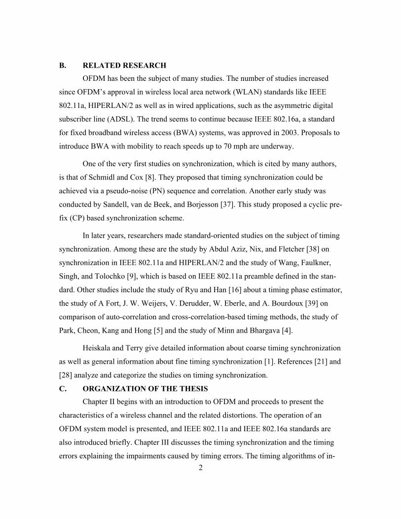
Now we have the time samples for one OFDM symbol. However, the data are not

yet ready to be sent through the channel. CP is needed to compensate for multi-path, ISI

and ICI. Figure 11 illustrates how the CP is appended to the OFDM symbol before enter-

ing the channel. The last part of the symbol is simply added to the beginning of the sym-

bol.

OFDM SymbolCP

Copy

OFDM SymbolCP OFDM SymbolCP OFDM SymbolCP

Copy

Figure 11. Adding CP to the OFDM Symbol

After the CP is added the signal goes through a parallel-to-serial converter (P/S),

which takes the data on the parallel sub-carriers and puts them into a row. Now, the sig-

nal is ready for transmission. The signal is sent through four different channels without

RF modulation. The channel characteristics are presented in Chapter IV.

As shown in Figure 9(b), in the receiver, after the S/P operation and removing CP,

an -pointN FFT is performed to obtain the received data symbol ( )my k as given below:

( ) ( )1

2 /

0

Nj kn N

m mn

y k r n e π−

−

=

= ∑ (2.18)

where ( )mr n denotes the received signal in time. The FFT operation is followed by dif-

ferential decoding, symbol-to-bit mapping, P/S operation, decoding and de-interleaving

operations.

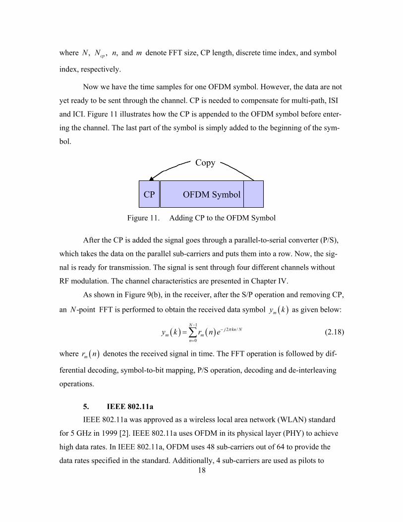
5. IEEE 802.11a IEEE 802.11a was approved as a wireless local area network (WLAN) standard

for 5 GHz in 1999 [2]. IEEE 802.11a uses OFDM in its physical layer (PHY) to achieve

high data rates. In IEEE 802.11a, OFDM uses 48 sub-carriers out of 64 to provide the

data rates specified in the standard. Additionally, 4 sub-carriers are used as pilots to

19

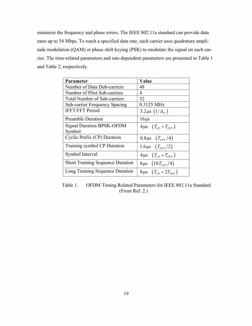
minimize the frequency and phase errors. The IEEE 802.11a standard can provide data

rates up to 54 Mbps. To reach a specified data rate, each carrier uses quadrature ampli-

tude modulation (QAM) or phase shift keying (PSK) to modulate the signal on each car-

rier. The time-related parameters and rate-dependent parameters are presented in Table 1

and Table 2, respectively.

Parameter Value Number of Data Dub-carriers 48 Number of Pilot Sub-carriers 4 Total Number of Sub-carriers 52 Sub-carrier Frequency Spacing 0.3125 MHz IFFT/FFT Period ( )3.2µs 1/ F∆ Preamble Duration 16µs Signal Duration BPSK-OFDM Symbol

( )4µs CP FFTT T+

Cyclic Prefix (CP) Duration ( )0.8µs 4FFTT Training symbol CP Duration ( )1.6µs 2FFTT Symbol Interval ( )4µs CP FFTT T+ Short Training Sequence Duration ( )8µs 10 4FFTT Long Training Sequence Duration ( )8µs 2CP FFTT T+

Table 1. OFDM Timing Related Parameters for IEEE 802.11a Standard

(From Ref. 2.)

20

Data Rate (Mbps) Modulation

FEC Coding Rate(R)

Coded Bits per Sub-carrier (NBPSC)

Coded Bits per OFDM

Symbol (NCBPS)

Data Bits per OFDM

Symbol (NDBPS)

6 BPSK 1/2 1 48 24 9 BPSK 3/4 1 48 36 12 QPSK 1/2 2 96 48 18 QPSK 3/4 2 96 72 24 16-QAM 1/2 4 192 96 36 16-QAM 3/4 4 192 144 48 64-QAM 2/3 6 288 192 54 64-QAM 3/4 6 288 216

Table 2. OFDM Rate Dependent Parameters for IEEE 802.11a Standard

(From Ref. 2.)

Table 3 presents the major parameters of the OFDM PHY. In this thesis, a data

rate of 24 Mbps with a FEC code rate of ½, and QPSK modulation were employed while

abiding by the other major parameters in Table 3.

Information Data Rate 6,9,12,18,24,36,48 and 54 Mbps (6,12 and 24 Mbps are Manda-tory)

Modulation BPSK OFDM QPSK OFDM 16-QAM OFDM 64-QAM OFDM

Error Correcting Code 7K = (64 states) Convolutional Code

Coding Rate 1/2, 2/3, 3/4 Number of Sub-carriers 52 OFDM Symbol Duration 4 µs Guard Interval ( )CP0.8 µs T Occupied Bandwidth 16.6 MHz

Table 3. Major Parameters of OFDM PHY for IEEE 802.11a Standard

(From Ref. 2.)

For synchronization purposes, a preamble consisting of short and long symbols is

given in the standard. The IEEE 802.11a preamble is presented in Figure 12, where 1t to

10t denote short training symbols, and 1T and 2T denote long training symbols.

21

Figure 12. IEEE 802.11a Preamble (After Ref. 2.)

6. IEEE 802.16a

IEEE 802.16a is a standard for fixed broadband wireless access systems for met-

ropolitan area networks (MAN) [6, 35], approved in 2003. The standard includes PHY

specifications and medium access control (MAC) modifications. The OFDM PHY layer

is one of the PHY layers specifications given in the standard and was designed for non-

line-of-sight (NLOS) communications in the frequency band 2-11 GHz. IEEE 802.16a

was intended for fixed wireless networks; however, IEEE 802.16 Task Group e (Mobile

Wireless MAN) is still working on an amendment to IEEE 802.16a for mobile wireless

MANs [26]. The IEEE 802.16-based systems, as an alternative to wired systems, are de-

signed to enable homes, offices, and small businesses as well as vehicles on the move to

access the networks. Several companies, such as Intel, Proxim, and Alvarion, have al-

ready begun developing equipment, such as hand-held devices and base stations, for

IEEE 802.16 and IEEE 802.16a systems [36].

Table 4 presents the symbol parameters for OFDM in IEEE 802.16a. In Table 4,

sF , gT , and bT denote the sampling frequency, the duration of the CP and the useful

symbol time before the CP addition, respectively. There are 192 data carriers and 8 pilot

carriers. One important issue to point out is that the length of the CP is not fixed in IEEE

802.16a. On initialization of communication between a base station and a subscriber sta-

tion, the subscriber station should search for all possible values for the CP [6]. Once the

subscriber station obtains the length of the CP, it uses the same length for the uplink

transmission. Table 5 provides channelization parameters for licensed bands in the US. It

can clearly be seen that the length of the OFDM symbol and the CP change when the

bandwidth changes.

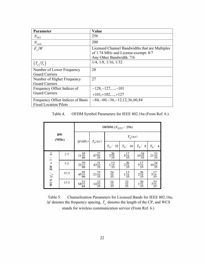
22

Parameter Value

FFTN 256

usedN 200

sF W Licensed Channel Bandwidths that are Multiples of 1.74 MHz and License-exempt: 8/7 Any Other Bandwidth: 7/6

( )g bT T 1/4, 1/8, 1/16, 1/32

Number of Lower Frequency Guard Carriers

28

Number of Higher Frequency Guard Carriers

27

Frequency Offset Indices of Guard Carriers

128, 127,..., 101101, 102,..., 127

− − −+ + +

Frequency Offset Indices of Basic Fixed Location Pilots

84, 60, 36, 12,12,36,60,84− − − −

Table 4. OFDM Symbol Parameters for IEEE 802.16a (From Ref. 6.)

Table 5. Channelization Parameters for Licensed Bands for IEEE 802.16a; f∆ denotes the frequency spacing, gT denotes the length of the CP, and WCS

stands for wireless communication service (From Ref. 6.)

23

C. SUMMARY

The fundamentals of OFDM were presented in this chapter. Also included were

the wireless channel characteristics as well as how OFDM deals with them. The wireless

channel is a multi-path channel causing ISI, ICI, and fading, and it has a time-varying

nature. OFDM effectively deals with ISI and ICI by employing a cyclic prefix. Using a

parallel transmission scheme mitigates the frequency selective fading. Parallel transmis-

sion also allows high data rates with high spectral efficiency. Besides mitigating channel

effects, OFDM has implementation advantages.

The structure of the OFDM scheme used in this thesis is also described. In the last

part of the chapter we introduced two standards that are using OFDM, a WLAN standard

IEEE 802.11a and a WMAN standard IEEE 802.16a.

The next chapter presents the need for timing synchronization and the effects of

timing errors. Following that, various timing synchronization methods are introduced.

24

THIS PAGE INTENTIONALLY LEFT BLANK

25

III. TIMING SYNCHRONIZATION AND INTRODUCTION OF ALGORITHMS

In this chapter, we present the need for timing synchronization in OFDM-based

systems, the effects of timing errors, and the distortions caused by these errors. The tim-

ing algorithms are also introduced in this chapter together with the results of simulations

conducted in an ideal channel environment.

A. THE NEED FOR TIMING SYNCRONIZATION AND TIMING ERRORS At the OFDM receiver, the signal initially goes through a synchronization process

before being demodulated into the frequency domain (this was not shown in Figure 9).

Besides timing synchronization, the synchronization process also includes synchroniza-

tion of the frequency, the sampling clock, and the phase. However, they are beyond the

scope of this study. The very first process the signal goes through is the coarse timing or

signal detection. The function of coarse timing is to detect the incoming signal and to ac-

tivate the receiver for the data. The coarse timing is not precise enough to determine the

actual start time of the symbols, so fine timing synchronization methods are required to

determine the actual start time of the symbol. Fine timing is crucial to reduce both the ICI

and ISI.

The purpose of the timing synchronization or the timing offset estimation is to

find a starting point for the FFT operation at the receiver. The importance of the accuracy

of such an estimate lies in the fact that ISI and ICI can be avoided. Figure 13 shows an

illustration of where ISI and ICI might occur in an OFDM system (also see Figure 7).

The ISI and ICI may occur under two conditions, assuming that there are no frequency

errors. The first condition is when we choose a sample close to the end of the CP as the

correct starting point of the FFT window, i.e., early timing, due to multi-path. This type

of ISI and ICI is illustrated as “ISI and ICI region 1” in Figure 13. When timing is esti-

mated in this region, ISI and ICI occur due to the delayed versions of the previous OFDM

symbol (see Section C of Chapter IV). The second condition is when we choose a sample

outside of the CP as the correct starting point, i.e., late timing. This type of ISI and ICI is

illustrated as “ISI and ICI region 2” in Figure 13.

26

Figure 13. Illustration of ISI and ICI in OFDM Systems

As mentioned earlier, having ISI from the previous symbol due to multi-path also

causes ICI. The distortion caused by ICI in this case is negligible. In a non-coherent de-

tection scheme, such as differential coding/decoding used in this thesis, there will be

some residual phase rotation due to ICI. In such systems, a timing phase estimator [16,

17] could be used to detect and to correct the phase rotation caused by ICI. Figure 14 il-

lustrates the effect of the ISI and ICI due to early synchronization, i.e, early timing, in

terms of bit error rate versus bit energy-to-noise ratio ( b oE N ) in dB. In this case, the

start of the FFT is chosen 6 points away from the region between the end of the CP and

the length of the channel impulse response. The simulation was run for 20,000 symbols

under Mobile Indoor Channel 1 with QPSK modulation (see Chapter IV for channel de-

scriptions). The data points on the plots are connected with a line. It can clearly be seen

that early timing degrades the BER. For the same BER, the case with early synchroniza-

tion requires about 0.5 dB more energy than the case with correct timing.

27

0 1 2 3 4 5 6 7 8 9 1010-4

10-3

10-2

10-1

100

Eb/No (dB)

BE

R

Correct timingEarly timing with an offset of 16 samples

Figure 14. The Effect of ISI and ICI due to Early Timing under Mobile Indoor

Channel 1

The effect of ISI and ICI due to late timing, however, can be more destructive

than early timing since, in the case of late timing, the OFDM symbol includes samples

from the CP of the next OFDM symbol. This effect can be thought of as a burst error.

The effect worsens as the number of foreign samples included in the FFT window in-

crease.

In order to avoid ISI in IEEE 802.11a systems, it is a rule of thumb to move the

estimated timing point back 4 to 6 samples [1]. The same rule can be used for other sys-

tems depending on the channel impulse response, the expected delay spread, the FFT

window, and the CP. We ran simulations (see Chapter IV) to see the effects of ISI and

ICI in the late timing case with a timing offset of100 ns , i.e., two samples. Figure 15 pre-

sents BER versus bit energy-to-noise ratio ( b oE N ) plots for correct timing and timing

offset of 100 ns in Mobile Indoor Channel 1 with QPSK modulation. The simulation was

run for 20,000 symbols. The data points on the plots are connected with a line. It can be

28

observed from the figure that the BER plot for this late timing is as much as 2 dB worse

than the BER plot for correct timing.

0 1 2 3 4 5 6 7 8 9 1010-3

10-2

10-1

100

Eb/No (dB)

BE

RLate timing with 100 nsCorrect timing

Figure 15. The Effect of ISI and ICI due to Late Timing with an Offset of 100 ns under

Mobile Indoor Channel 1 B. COARSE TIMING

The function of coarse timing is to find the start of an incoming data packet. In

packet switched networks, each packet has a preamble. The IEEE 802.11a and IEEE

802.16a packets also have preambles designed to ease various tasks as well as synchroni-

zation [2, 6]. In an OFDM system, the very first algorithm to run is the coarse timing al-

gorithm [2, 6], and the rest of the tasks rely on the performance of this algorithm.

Coarse timing can be defined as a binary hypothesis test consisting of two state-

ments: the null hypothesis, 0H , and the alternative hypothesis, 1H [1]. To set up the test,

we need a metric ( )M n , i.e., a decision variable, and a threshold, γ , to test against. The

test is defined as

( )( )

0

1

: Packet not present: Packet present.

H M nH M n

λγ

< ⇒≥ ⇒

29

Coarse timing is characterized by two probabilities, probability of detection of a

packet, ,dP given the fact that a packet is present and the probability of false alarm, ,faP

i.e., detecting a packet when there is no packet. Intuitively, the probability of a false

alarm should be as small as possible. However, there is a trade-off between having a

low faP and a high dP . Increasing one of them causes the other one to increase [1]:

.

d fa

d fa

P P

P P

↑⇔ ↑

↓⇔ ↓

Reference [1] presents two algorithms for coarse timing. The first one is based on

a measure of the energy of the incoming data. In this case, there is no need to have a spe-

cifically designed preamble or a training symbol. In the absence of data, the received sig-

nal would be made of only AWGN samples, which are uncorrelated to each other. In the

equations below, ( )r n , ( )s n , ( )w n denote the received signal, the data and the AWGN,

respectively, and they are related as

( ) ( )( ) ( )

in the absence of data in the presence of data.

w nr n

s n w n

= + (3.1)

The accumulation of the energy of the signal over a window will result in small

values for AWGN, and there will be a rise in the energy level ( )E n after the start of the

packet edge. This can be expressed as

( ) ( ) ( )1 2

0

L

m

M n E n r n k−

=

= = −∑ . (3.2)

where L is the length of the window.

Clearly, the metric ( )M n depends on the energy of the data sent. A sliding win-

dow scheme is used to obtain the energy of the signal. Figure 18 shows a plot for the en-

ergy of the signal over a window length of 32 samples. The simulation was run in the

AWGN channel with 10 dBb oE N = . The transmitter sends its first symbol of a 1200-bit

packet after 4 µs of null transmission, i.e., transmission of all zeros for 4 µs . The packet

starts at the sample number 80. The timing metric takes its first value at sample 48, which

is 32 samples away from the starting point of the packet. After the exact starting point at

sample 80, the timing metric tends to be flat.

30

0 20 40 60 80 100 1200

5

10

15

20

25

30

Sample Number

Tim

ing

Met

ric

Figure 16. Detection by Energy over a Window

The crucial point at this stage is to set up a reliable threshold, since the threshold

determines faP and dP of the test. In [7], dP is given as

( )( )max

d

M nP Q

λσ

−=

, (3.3)

where the Q -function is defined as

( ) 2 / 212

y

z

Q z e dyπ

∞−= ∫ , (3.4)

and

( )0 0Pr x m x my Q Q zσ σ− − > = =

. (3.5)

Another method discussed in [1] is a double sliding window method for which

there are two windows, A and B, of the same length. In the absence of data, the response

31

to the algorithm is flat. In this case, both windows collect ideally the same amount of

noise energy. As the packet edge enters window A, the metric gradually increases until

the packet reaches window B. The metric continuously decreases as the packet goes

along window B. After window B is completely inside the packet, we expect the metric

to be flat again. This phenomenon can be observed in Figure 17.

Figure 17. Illustration of Double Sliding Window Detection Algorithm (After Ref. 1.)

The equations below show how the double sliding window algorithm works. Let

( ) ( )( )

a nM n

b n= (3.6)

where

( ) ( )1 2

0

L

k

a n r n k−

=

= −∑ (3.7)

and

( ) ( ) 2

0

L

k

b n r n k=

= +∑ . (3.8)

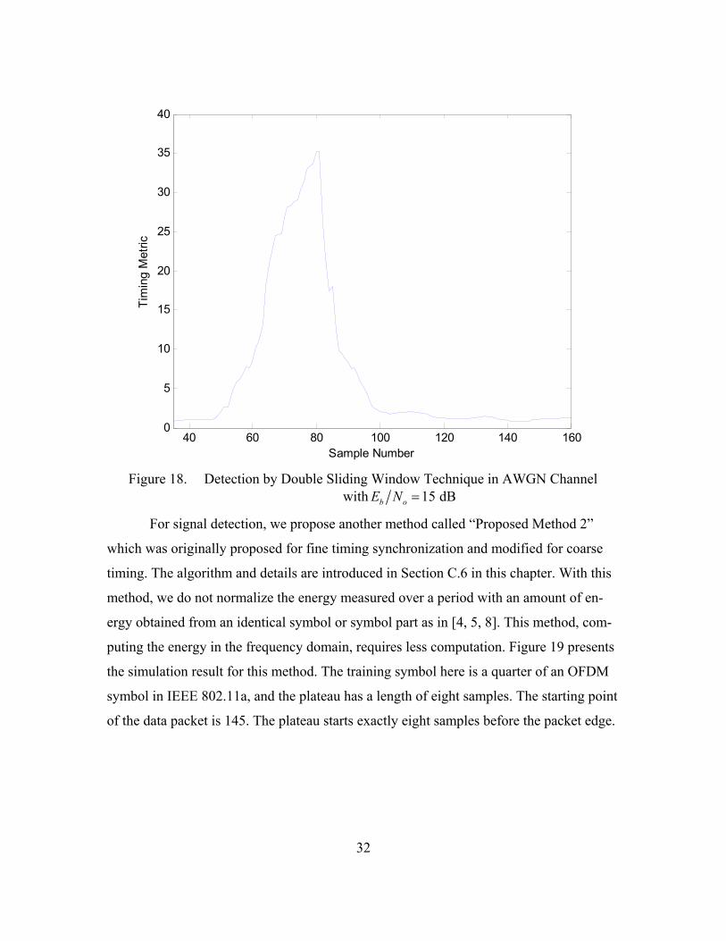
Figure 18 shows the simulation result for a double sliding window technique with

15 dBb oE N = in AWGN channel. In this example, the A and the B windows have a

length of 32 samples. The triangle shape can clearly be observed beginning from sample

number 48 and ending around sample number 112. These two numbers are the outer

edges of the two windows when the timing metric reaches its peak. The start of the

packet is sample number 80, where the timing metric has its peak. So, if we set a thresh-

old around the timing metric value of 20, we will have an early detection. However, this

does not affect the performance of the system since the symbol start time is to be detected

by fine timing synchronization.

( )M n

A B

Packet

----------------------- Th

32

40 60 80 100 120 140 1600

5

10

15

20

25

30

35

40

Sample Number

Tim

ing

Met

ric

Figure 18. Detection by Double Sliding Window Technique in AWGN Channel

with 15 dBb oE N =

For signal detection, we propose another method called “Proposed Method 2”

which was originally proposed for fine timing synchronization and modified for coarse

timing. The algorithm and details are introduced in Section C.6 in this chapter. With this

method, we do not normalize the energy measured over a period with an amount of en-

ergy obtained from an identical symbol or symbol part as in [4, 5, 8]. This method, com-

puting the energy in the frequency domain, requires less computation. Figure 19 presents

the simulation result for this method. The training symbol here is a quarter of an OFDM

symbol in IEEE 802.11a, and the plateau has a length of eight samples. The starting point

of the data packet is 145. The plateau starts exactly eight samples before the packet edge.

33

Figure 19. Signal Detection by Proposed Method 2

Signal detection is not complex and is fairly easy to understand and to implement.

Most of the techniques used for fine timing synchronization, i.e., symbol timing, can be

used for coarse timing as well.

C. FINE TIMING In this section, the fine timing methods of interest are described. In all, six timing

methods are introduced.

1. Schmidl and Cox Method In Schmidl and Cox method [8], timing synchronization is achieved by using a

training sequence whose first half is equal to its second half in the time domain. The ba-

sic idea behind the technique is that the symbol timing errors will have little effect on the

signal itself as long as the timing estimate is in the CP.

The two halves of the training sequence are made identical by transmitting a PN

sequence on the even frequencies while zeros are sent on the odd frequencies. When we

take the IFFT of this sequence, the property of being identical can be seen. Another way

0 50 100 150 200 250 300 3500

0.2

0.4

0.6

0.8

1

1.2

1.4

1.6

1.8

2

Sample Number

Tim

ing

Met

ric

34

of achieving this training symbol with two identical halves is to use a PN sequence of

half the symbol length (32 points for the case of IEEE 802.11a), take the IFFT of it, and

then repeat it. As stated in [8], one advantage of sending zeros on odd frequencies is that,

especially in continuous broadcasting systems like DVB, this property could be used to

distinguish the training symbol from the data since the data would have values on the odd

frequencies. Table 6 shows a PN sequence for the training symbol. However, in [8], a

different PN sequence whose values are taken from a 64-QAM constellation is used.

Frequency Number ( )2 km0 1 1*i+ 1 0 2 1 1*i− +3 0 4 1 1*i+ 5 0 6 1 1*i− 7 0 8 1 1*i+ 9 0

Table 6. PN Sequence for Training Symbol for the Method in [8]

Let N be the number of complex samples in one OFDM symbol. The algorithm

defined in [8] has three steps, based on the following equations:

( ) ( ) ( )( )( / 2) 1

*

0/ 2

N

k

P n r n k r n k N−

=

= + + +∑ . (3.9)

( ) ( )( / 2) 1

2

0

/ 2N

k

R n r n k N−

=

= + +∑ . (3.10)

( ) ( )( )( )

2

2

P nM n

R n= . (3.11)

In Equation 3.9, the algorithm has a window length of N , which is also the num-

ber of sub-carriers. The starting point is the value of n , which maximizes ( )M n . In fact,

from the definition, ( )P n expresses the cross-correlation between the two halves of the

35

window; in Equation 3.10, ( )R n represents the auto-correlation of the second half. When

the starting point of the window reaches the start of the training symbol with the CP, the

values of ( )P n and ( )R n should be equal giving the maximum value for the timing

metric as defined in Equation 3.11.

Under ideal conditions, when there is no channel effect and no noise, the timing

metric gives a plateau of width equal to the CP. In order to see how the algorithm works,

we implemented the algorithm and obtained the timing metric. Figure 20 shows the tim-

ing metric under ideal channel conditions. It is obvious that the plateau starts at the sam-

ple 81, which is the starting point of the CP, and the plateau runs till the sample 97,

which is the start of the symbol. The length of the plateau should reduce down to the CP

minus the length of the channel impulse response under the actual conditions.

0 20 40 60 80 100 120 1400

0.2

0.4

0.6

0.8

1

1.2

1.4

Sample Number

Tim

ing

Met

ric

Figure 20. Timing Metric for Schmidl and Cox Method under Ideal Conditions with No

Channel Effect and No Noise

36

There are two methods to determine the symbol timing. The first one is just to

find the maximum of the metric. The second one is to find the maximum, and the points

to the left and right that are 90% of the maximum and then compute the average of these

two 90% points to find the symbol timing estimate. The second method is more desirable

when the metric has a plateau as shown in Figure 20.

2. Minn and Bhargava Method

In [4], Minn and Bhargava present another method to reduce the uncertainty that

[8] has in finding the correct timing. They propose an OFDM training symbol to be of the

form given by

-S/4-S/4S/4S/4s =

where 4S represents the 4N point IFFT of a modulated PN sequence. The chosen PN

sequence is given in Table 7.

Frequency Number PN Sequence Frequency Number PN Sequence

0 1 1*i+ 8 1 1*i− + 1 1 1*i− + 9 1 1*i− 2 1 1*i− − 10 1 1*i+ 3 1 1*i− 11 1 1*i− 4 1 1*i+ 12 1 1*i− 5 1 1*i− 13 1 1*i− + 6 1 1*i− + 14 1 1*i+ 7 1 1*i− + 15 1 1*i− +

Table 7. PN Sequence to Obtain the Training Symbol in [4]

The cross-correlation sequence between the positive-valued and negative-valued

parts of the training symbol is given by

( ) ( ) ( )1 1

*2

0 0

2 2L

k m

P n r n Lk m r n Lk m L−

= =

= + + + + +∑∑ , (3.12)

and the auto-correlation sequence of the second positive-valued and negative-valued parts

of the symbol

( ) ( )1 1 2

20 0

2L

k m

R n r n Lk m L−

= =

= + + +∑∑ (3.13)

37

where L is the length of 4S . Finally, the timing metric is given by

( ) ( )( )( )

22

2 22

P nM n

R n= . (3.14)

Equation 3.13 basically calculates half symbol energy using 2N samples. This

equation can be replaced by

( ) ( )1 2

2.10

12

N

m

R n r n m−

=

= +∑ . (3.15)

In our simulations, we used Equation 3.15.

The idea behind this method is to avoid the plateau we found in [8] and shown in

Figure 20. Another point to note is that the results are based on 1,024 sub-carriers and

10% of the OFDM symbol as CP, which corresponds to 102 samples. This technique is

not directly applicable to IEEE 802.11a since there are only 64 sub-carriers and the CP is

16 samples that correspond to one-fourth of the OFDM symbol itself. In the simulations,

we did not add the CP. Adding the CP causes the timing metric to have more peaks.

Figure 21 shows the timing metric under ideal channel conditions. The middle

peak is the peak of interest. In this simulation, the starting point of the training symbol is

sample 96, where the timing metric has a peak with the magnitude of 1.

38

75 80 85 90 95 100 105 110 1150

0.2

0.4

0.6

0.8

1

Sample Number

Tim

ing

Met

ric

Figure 21. Timing Metric for Minn and Bhargava Method [4] under Ideal Conditions

with No Channel Effect and No Noise

3. Park et al. Method The third method we studied was proposed by Park et al. [5]. The training symbol

used in this method is given by

where 4S represents time samples of length 4N formed by IFFT of a PN sequence,

and *4A represents the time-reversed conjugate of 4S . This symbol can easily be ob-

tained by having a real-valued PN sequence on the even frequencies and zeros on the odd

frequencies and applying the IFFT operation to this sequence. A new algorithm is pro-

posed to exploit the symmetric property of the above training symbol. The cross-

39

correlation sequence, the auto-correlation sequence, and the timing metric, respectively,

are given by

( ) ( ) ( )/ 2

30

N

k

P n r n k r n k=

= − +∑ , (3.16)

( ) ( )/ 2 2

30

N

k

R n r n k=

= +∑ , (3.17)

( ) ( )( )( )

23

3 23

P nM n

R n= . (3.18)

The idea behind the symmetric property of this algorithm is to have only one mu-

tual product for each n value. Therefore, the estimation of the timing occurs at the de-

sired correct symbol timing while other values approach zero.

In this method, although the peak occurs exactly at the correct timing, we found

that its peak magnitude is very sensitive to AWGN and indoor multi-path channels,

which makes the estimation over a threshold difficult. We further discuss this issue in

Chapter IV.

Figure 22 presents the plot for the timing metric under ideal channel conditions.

The desired starting point is 129, and the delta function-like shape of the timing metric

can clearly be seen at the exact starting point. The timing metric for this method has a

narrower peak than both methods discussed earlier (see Figures 20 and 21).

40

60 70 80 90 100 110 120 130 140 150 1600

0.1

0.2

0.3

0.4

0.5

0.6

0.7

0.8

0.9

1

Sample Number

Tim

ing

Met

ric

Figure 22. Timing Metric for Park et al. Method under Ideal Conditions with No Chan-

nel Effect and No Noise 4. Wang et al. Method The fourth method in our study is presented in [9]. It employs the preamble given

in the IEEE 802.11a standard (see Figure 12). In this method, fine synchronization is

achieved through two steps, coarse timing and fine timing. The term coarse timing is

used here in the sense that it provides a reference point as to where to start the fine timing

process. In coarse timing, there are two metrics to define:

( )( ) ( )

( )

1

01 1

2

0

*s

s

N

sm

N

m

r n m r n m Nm n

r n m

−

=−

=

+ + +=

+

∑

∑, (3.19)

( )( ) ( )

( )

1

02 1

2

0

2 *s

s

N

sm

N

m

r n m r n m Nm n

r n m

−

=−

=

+ + +=

+

∑

∑. (3.20)

41

The first metric ( )1m n is the normalized auto-correlation between the received

signal and a delayed version with the delay equal to sN , where 16sN = . It gives us a pla-

teau of nine short symbols. The second metric ( )2m n has the same properties except for

32sN = , i.e., the length of two short symbols. It gives us a plateau of eight short sym-

bols. The actual metric we use for detection is given by

( ) ( ) ( )4 1 2M n m n m n= − . (3.21)

The coarse timing can be achieved by searching the maximum point in ( )4M n .

Figure 23 and 24 shows the metrics. The metric ( )1m n in Figure 23 has a plateau of 8

short symbols whereas the metric ( )2m n has a plateau of 9 short symbols. The metric

( )4M n in Figure 24 shows the result of the subtraction operation in Equation 3.21.

0 50 100 150 200 2500

0.5

1

1.5

Sample Number

Tim

ing

Met

ric

0 50 100 150 200 2500

0.5

1

1.5

Sample Number

Tim

ing

Met

ric

(a) (b)

Figure 23. Metrics: (a) 1( )m n and (b) 2 ( )m n

42

0 50 100 150 200 250

-0.2

0

0.2

0.4

0.6

0.8

1

1.2

1.4

Sample Number

Tim

ing

Met

ric

Figure 24. Coarse Timing Metric ( )4M n

In [9], it is claimed that even if this metric is well localized in time, it may not

perform well since the peak could be off. Therefore, this process needs another step,

which is fine timing. Fine timing is realized by using long training symbols. For fine tim-

ing, they use a method that has been studied in [19, 42] for continuous transmission to

estimate the channel response. The least squares estimation of the channel frequency re-

sponse can be expressed as [9]

( ) , ( )( )

0,

uLS

u

Y k k NX kH k

k N

∈= ∉

(3.22)

where ( )H k is the channel frequency response at the sub-carrier k , ( )Y k is the -thk

sample of the received long training symbol, ( )LSX k is the -thk sample of the transmit-

ted long training symbol, and uN is the number of sub-carriers in the long training sym-

43

bols. In IEEE 802.11a there are 53 sub-carriers in the long training symbols. After obtain-

ing ( )H k , it is easy to find the channel impulse response ( )h i as given by

( ) ( )21

0, 0,1,..., 1.

j kiNN

kh i H k e i N

π−

=

= = −∑ (3.23)

At this point, optimum timing synchronization can be applied as discussed in [28], in the

presence of multi-path channels, to find the path delay. The starting time of the symbol is

defined as the starting time of a window with the length of CP, which contains the maxi-

mum power of the estimated channel impulse response. If the channel impulse length is

shorter than the CP, the window size may be reduced to the channel length. The optimum

timing can be found by searching for the maximum value in ( )5M i given by

( ) ( )1

25

0

sN

j

M i h i j−

=

= +∑ (3.24)

where sN represents the size of the window.

5. Proposed Method 1 (a Modification of the Park et al. Method)

Here we propose a new method to prevent the peak degradation in [5] due to the

distortion by AWGN. We define a new symbol form given by

where 4S represents a 16-point IFFT of a PN sequence, and 4A is defined to be sym-

metric with 4S . The metric, cross-correlation sequence and the auto-correlation se-

quence are given as follows:

( ) ( )( )( )

26

6 26

P nM n

R n= , (3.25)

where

( ) ( ) ( )/ 2 1

60

1N

k

P n r n k r n k−

=

= − + +∑ , (3.26)

and

( )21

60

12

N

k

NR n r n k−

=

= − + +

∑ . (3.27)

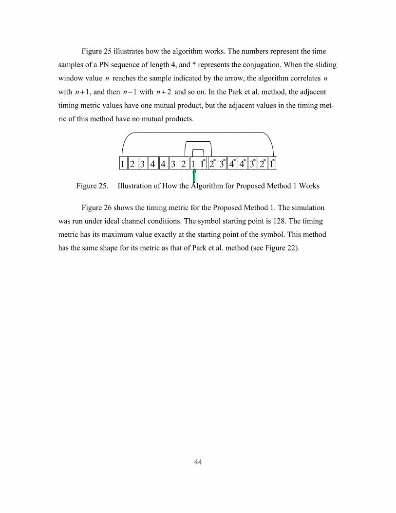
44

Figure 25 illustrates how the algorithm works. The numbers represent the time

samples of a PN sequence of length 4, and * represents the conjugation. When the sliding

window value n reaches the sample indicated by the arrow, the algorithm correlates n

with 1n + , and then 1n − with 2n + and so on. In the Park et al. method, the adjacent

timing metric values have one mutual product, but the adjacent values in the timing met-

ric of this method have no mutual products.

Figure 25. Illustration of How the Algorithm for Proposed Method 1 Works

Figure 26 shows the timing metric for the Proposed Method 1. The simulation

was run under ideal channel conditions. The symbol starting point is 128. The timing

metric has its maximum value exactly at the starting point of the symbol. This method

has the same shape for its metric as that of Park et al. method (see Figure 22).

* * * * * * * *1 2 3 4 4 3 2 1 1 2 3 4 4 3 2 1

45

50 60 70 80 90 100 110 120 130 140 1500

0.1

0.2

0.3

0.4

0.5

0.6

0.7

0.8

0.9

1

Sample Number

Tim

ing

Met

ric

Figure 26. Timing Metric for Proposed Method 1 under Ideal Conditions with No

Channel Effect and No Noise

6. Proposed Method 2 The final method we present is a cross-correlation based method. We offer two

slightly different algorithms here. The first one is designed to be used for fine timing, and

the second one is designed for coarse timing. However, either one may be used for both

coarse timing and fine timing.

Let ( )r n be the received signal, and ( )s n be the transmitted signal. The transmit-

ted signal ( )s n is given by

S/4s = S/4s =

where 4S represents the IFFT of the training sequence as shown in Table 8.

46

Frequency Number PN Sequence Frequency Number PN Sequence 0 7 7*i+ 8 7 7*i− + 1 7 7*i+ 9 7 7*i− 2 7 7*i− − 10 7 7*i+ 3 7 7*i− 11 7 7*i− 4 7 7* i+ 12 7 7*i− 5 7 7*i− 13 7 7*i− + 6 7 7*i− + 14 7 7*i+ 7 7 7*i− + 15 7 7*i− +

Table 8. PN Sequence to Obtain the Training Sequence 4S

The FFT of the received and the transmitted signals are given by:

( ) ( ){ }FFT : 16R k r n n= + , (3.28)

( ) ( ){ }FFTS k s n= . (3.29)

The cross-correlation between ( )r n and ( )s n can be obtained as

( ) ( ) ( ){ }*IFFTl S k R kϒ = . (3.30)

Finaly, the timing metric is given by ( ) ( )7 maxM n l= ϒ . (3.31)

Equation 3.28 represents a sliding FFT window with the length of 16, which

comes from the length of the transmitted signal ( )s n . After implanting the algorithm, we

observed that the metric ( )7M n reaches its maximum value exactly at the desirable

point. Figure 27 presents the timing metric under ideal channel conditions. The symbol

starting point is 144 in this simulation. The timing metric has its peak at 144 while there

are no other peaks present.

47

0 50 100 150 200 250 300 3500

10

20

30

40

50

60

70

80

90

100

Figure 27. Timing Metric for Proposed Method 2 for Fine Timing (first algorithm)

The second algorithm as part of the Proposed Method 2 is more suitable for

coarse timing since it can reach a plateau in a few samples and keep its maximum value

for several samples. The length of the plateau can be determined by the designer. It pro-

vides enough time to determine the presence of the signal, and the peak is strong enough

to exceed a threshold, even under severe channel conditions and low values ofSNR .

This algorithm differs from the one presented above in the structures of the

transmitted and the known training sequences. The same training symbol as in the first

algorithm is used.

Let ( )s n be training sequence known by the receiver and given by

(3.32)

48

The FFT of the received signal ( )r n and the training sequence ( )s n known by the re-ceiver are given by

( ) ( ){ }FFT : 20R k r n n= + , (3.33)

( ) ( ){ }FFTS k S n= (3.34)

where the length of the FFT window is 20 due to the zero padding in ( )s n in Equation

3.32. The cross-correlation between ( )r n and ( )s n can be obtained as

( ) ( ) ( ){ }*IFFTl S k R kϒ = . (3.35)

The same metric in the first algorithm is used.

The length of the plateau can be changed by altering the length of zero padding in

Equation 3.32. Figure 28 shows the timing metric for the second algorithm. The plateau

in Figure 28 has a length of four samples, which is the length of zero padding in Equation

3.32. The packet starts at the sample number 144. Both of the algorithms introduced in

this method can be implemented with longer PN sequences.

49

0 50 100 150 200 250 300 3500

10

20

30

40

50

60

70

80

90

100

Sample Number

Tim

ing

Met

ric

Figure 28. Timing Metric for Proposed Method 2 for Coarse Timing (second algo-

rithm) D. SUMMARY

In this chapter, we presented the need for timing synchronization, the effects of

timing errors on the performance of the OFDM system, and the methods used for timing

synchronization. We also provided the performance plots for algorithms in a noise-free

environment without any channel effects. The next chapter presents the performances of

timing synchronization methods in time-varying, multi-path indoor, and outdoor chan-

nels.

50

THIS PAGE INTENTIONALLY LEFT BLANK

51

IV. OFDM SYSTEM SIMULATIONS IN MATLAB

In Chapters II and III, we covered the fundamentals of OFDM, the basics of two

OFDM-based standards in use, the importance of timing in OFDM systems, the timing

errors, and their effects. Additionally, we introduced several algorithms presented by

various authors and researchers as well as two new algorithms. This chapter presents a

Matlab simulation of an OFDM system that operates under different channel conditions

and the performances of the timing methods.

A. SELECTING SYSTEM PARAMETERS

The Matlab simulation used in this thesis is based on the IEEE 802.11a standard.

The standard allows different modulation schemes [2]. We chose QPSK, which gives us a

bit rate of 12 Mbps, i.e., an operational bit rate of 24 Mbps due to the FEC rate of 1/2.

The bit rate is calculated as follows:

bits per OFDM symbol FEC rate 96 bits/sym 0.5bit rate 12 MbpsOFDM symbol time 4 sµ

× ×= = = (4.1)

Without considering the coherence bandwidth issue and channel effects, the effi-

cient bandwidth usage in OFDM can be observed when we calculated the required band-

width for the same bit rate for QPSK modulation, using

2 2 /nn s bW R R k= = (4.2)

where nnW denotes null-to-null bandwidth required, sR denotes symbol rate, bR denotes

bit rate, and k stands for bits per symbol. When we put the numbers in the equation we

get 24 MHznnW = . The standard gives the occupied bandwidth as 16.6 MHz , and the

bandwidth efficiency can be calculated as

24Mbps 1.44bit/s/Hz.16.6MHz

= (4.3)

The symbol interval given in the standard is 4µs, and the sub-carrier spacing

given is 0.3125MHz [2], which is obtained from the standard as

20 MHz 0.3125 MHz.64

= (4.4)

52

However, all of the 64 carriers are not used for transmission. The standard gives

the number of sub-carriers as 52, 4 of which are assigned as pilot sub-carriers and 48 of

which are assigned as data carriers. The calculation is as follows:

occupied bandwidth 16.6MHz 53.frequency spacing 0.3125 MHz

N = = = (4.5)

The 53rd sub-carrier is used only for long training symbols in the 802.11a preamble de-

fined in the standard [2]. The 4 pilots are used for detecting frequency and phase errors.

The CP has 16 samples that correspond to800 ns . One OFDM symbol ready for

transmission consists of 80 samples representing 4 µs in time as in the standard. The

other parameters can be seen in Table 1 in Chapter II.

B. SIMULATION METHODOLOGY The code used in simulation is based on [12] and modified later on by [13]. We

did not change the basic structure of the code. Before adding our required sub-blocks for

each of the timing algorithms, we ran simulations under different channel models to see if

the code is correct and reliable. The simulation steps performed are presented in Figure

29.

53

Noiseless channelsimulations

AWGN channelsimulations

Mobile Indoorchannel simulations

Mobile Indoorchannel simulations

Simulations of Timing Algorithms

Noiseless channelsimulations

AWGN channelsimulations

Mobile Indoorchannel simulations

Mobile Indoorchannel simulations

Simulations of Timing Algorithms

Figure 29. Matlab Simulations Scheme

We assumed a similar simulation process as in [13]. First we ran the code under

ideal conditions, i.e., without noise and channel effects, to verify the code. After verifica-

tion, we ran simulations for an AWGN channel, two mobile indoor channels and two

mobile outdoor channels. The characteristics of these channels are presented in this chap-

ter. Before the timing-related simulations were conducted, the performance of the system

was investigated to show how mobile channels affect the system. As the final step, we

simulated each of the timing methods under different channels to see the channel effects

on the timing. From the results, it can be observed which channel affects the system more

severely. Table 9 presents the simulation steps.

54

Order

No.

Simulation Channel Description

1. Code Check Channel without AWGN and

Multi-path Effects (Ideal channel).

2. Performance in AWGN AWGN Channel

3. Performance in Mobile

Channels

Multi-path + AWGN Channel

4. Performance of Timing

Methods

a. AWGN Channel

b. Mobile Indoor Channels

c. Mobile Outdoor Channels

Table 9. The Order in Which the Simulations are Executed

The approach in Table 9 allowed us to see how different communication envi-

ronments can affect a real system and to make comparisons and inferences to have a

deeper understanding of OFDM and the channel effects on it. We used this knowledge to

better understand the channel effects on timing methods.

The verification of the code and the results are presented below.

1. Code Check (Ideal Channel) We checked the code in an ideal channel free from noise and any channel effects.

With no distortions affecting the channel, the receiver should receive exactly what the

transmitter sends. The simulations were run employing QPSK and 8-PSK modulations.

The results showed that the system functioned correctly.

Table 10 lists the parameters of a simulation run for QPSK and 8-PSK implemen-

tations, respectively. It can be seen from Figure 30 and 31 that the receiver constellations

are the same as those of the transmitters.

55

[42 24]33481000Ideal QPSK

[42 24]33481000Ideal 8-PSK

Interleaverblock size

Seed# of data carriers

# of symbols

Channel model

Modulation

[42 24]33481000Ideal QPSK

[42 24]33481000Ideal 8-PSK

Interleaverblock size

Seed# of data carriers

# of symbols

Channel model

Modulation

Table 10. Code Check Simulation Parameters for QPSK and 8-PSK

-1.5 -1 -0.5 0 0.5 1 1.5-1.5

-1

-0.5

0

0.5

1

1.5

Real

Imag

inar

y

-1.5 -1 -0.5 0 0.5 1 1.5-1.5

-1

-0.5

0

0.5

1

1.5

Real

Imag

inar

y

(a) (b)

Figure 30. (a) Transmitted and (b) Received QPSK Constellations for Ideal Channel Conditions

-1.5 -1 -0.5 0 0.5 1 1.5-1.5

-1

-0.5

0

0.5

1

1.5

Real

Imag

inar

y

-1.5 -1 -0.5 0 0.5 1 1.5-1.5

-1

-0.5

0

0.5

1

1.5

Real

Imag

inar

y

(a) (b)

Figure 31. (a) Transmitted and (b) Received 8-PSK Constellations for Ideal Channel Conditions

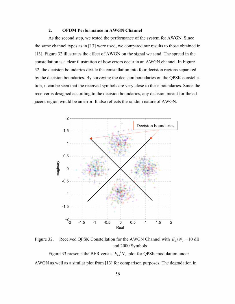
56

2. OFDM Performance in AWGN Channel As the second step, we tested the performance of the system for AWGN. Since

the same channel types as in [13] were used, we compared our results to those obtained in

[13]. Figure 32 illustrates the effect of AWGN on the signal we send. The spread in the

constellation is a clear illustration of how errors occur in an AWGN channel. In Figure

32, the decision boundaries divide the constellation into four decision regions separated

by the decision boundaries. By surveying the decision boundaries on the QPSK constella-

tion, it can be seen that the received symbols are very close to these boundaries. Since the

receiver is designed according to the decision boundaries, any decision meant for the ad-

jacent region would be an error. It also reflects the random nature of AWGN.

-2 -1.5 -1 -0.5 0 0.5 1 1.5 2-2

-1.5

-1

-0.5

0

0.5

1

1.5

2

Real

Imag

inar

y

Decision boundaries

-2 -1.5 -1 -0.5 0 0.5 1 1.5 2-2

-1.5

-1

-0.5

0

0.5

1

1.5

2

Real

Imag

inar

y

Decision boundaries

Figure 32. Received QPSK Constellation for the AWGN Channel with 10 dBb oE N =

and 2000 Symbols

Figure 33 presents the BER versus b oE N plot for QPSK modulation under

AWGN as well as a similar plot from [13] for comparison purposes. The degradation in

57

communication can clearly be seen as b oE N decreases. Figure 34 illustrates the magni-

tude variation in AWGN channel. Figure 34(b), having random peaks and dips, illustrates

the magnitude degradation and the randomness contributed by the AWGN.

-1 0 1 2 3 4 5 6 7 8 9

10-4

10-3

10-2

10-1

100

Eb/No(dB)

BE

R

(a) (b)

Figure 33. BER Plots for QPSK Simulation in AWGN Channel (a) From Ref. 13, (b) Simulated

010

2030

4050

0

10

20

300

0.5

1

1.5

2

OFDM Subcarrier NumberSymbol Row Number

Sig

nal M

agni

tude

010

2030

4050

0

10

20

300

0.5

1

1.5

2

OFDM Subcarrier NumberSymbol Row Number

Sig

nal M

agni

tude

(a) (b)

Figure 34. Magnitude Variation in AWGN Channel with 10 dBb oE N = , (a) Trans-

mitted Packet, (b) Received Packet

58

3. Performance under Mobile Channels We used two channel types, indoor and outdoor channels. Each type has two

channels. The channels are: Mobile (indoor) channel 1, mobile (indoor) channel 2, mo-

bile (outdoor) channel 3, and mobile (outdoor) channel 4. The distinction between them

is the number of paths, the relative velocity of the receiver, i.e., Doppler frequency, and

the delay lengths and different filters. The major characteristics are presented later in this

section.

a. Mobile Indoor Channels

Mobile indoor channels (Mobile Indoor Channel 1 and Mobile Indoor

Channel 2) are characterized by frequency selective fading, 18 multi-path components,

delays associated with multi-path components, Doppler frequency shift and AWGN. Mo-

bile Indoor Channel 1 and Mobile Indoor Channel 2 differ from each other by having dif-

ferent Doppler shifts. The characteristics are given in the m-file called cofdmsim in Ap-

pendix A. The indoor channels have 4 parallel 7th-order linear finite impulse response

(FIR) filters with 8 taps [11]. The coefficients of the filters are taken from [14]. These

filters can be found in m-file called cvdd in the code in Appendix A. Figure 35 gives a

schematic of the filters. The filter coefficients assigned for the four FIR filters are tabu-

lated in Table 11.

Figure 35. Modeling of Mobile Indoor Channels Using FIR Filters and Delay Elements

D (From Ref. 13.)

59

c 0 1 2 3 4 5 6 7

0a −0.013824 0.054062 −0.157959 0.616394 0.616394 −0.157959 0.054062 0.013824

1a 0.003143 −0.019287 0.1008 −1.226364 1.226364 −0.1008 0.019287 −0.003143

2a 0.055298 −0.216248 0.631836 −0.465576 −0.465576 0.631836 −0.216248 0.055298

3a −0.012573 0.077148 −0.403198 0.905457 −0.905457 0.403198 −0.077148 0.012573

Table 11. FIR Filter Coefficients for Indoor Channels

b. Mobile Outdoor Channels

In mobile outdoor channels there are a smaller number of multi-path com-

ponents. This type of channel is modeled using 6-tap FIR filters. They are also character-

ized with time-varying coefficients based on Jakes spectrum [15]. The major characteris-

tics of channels are shown in Tables 12 and 13. The parameters specified in Tables 13

and 15 can be changed to reflect the desired channel characteristics.

654321Path No

000000Ricean factor

201510910Power losses (dB)

2.201.910.50.250Time delays (ms)

654321Path No

000000Ricean factor

201510910Power losses (dB)

2.201.910.50.250Time delays (ms)

Table 12. Mobile Outdoor Channel 3 Parameters with 200 Hzdf =

60

654321Path No

00000.50.5Ricean factor

1625.2109002.5Power losses (dB)

20171390.250Time delays (ms)

654321Path No

00000.50.5Ricean factor

1625.2109002.5Power losses (dB)

20171390.250Time delays (ms)

Table 13. Mobile Outdoor Channel 4 Parameters with 200 Hzdf =

c. Channel Simulations The purpose of the channel simulations was to see channel behaviors and

their effects on the signal. These simulations have also enabled us to compare the chan-

nels in terms of the distortion that they cause. This is very beneficial to the concept be-

hind this study, since our goal was to see the performances of different timing algorithms

for various channels with different characteristics. The four mobile channel models with

different characteristics were simulated, and the performance plots are presented later in

this section. Table 14 presents the parameters used for simulations in this section. QPSK

and 8-PSK modulation schemes with frequency differential coding were employed for

each channel model with 40,000 symbols and 10 dBb oE N = .

Frequency

Frequency

Dif.Coding

[278 139]1033400001,2,3,4QPSK

10 [278 139]33400001,2,3,48PSK

Interleaverblock size

Seed# of symbols

Channel model

Modulation obE N

Frequency

Frequency

Dif.Coding

[278 139]1033400001,2,3,4QPSK

10 [278 139]33400001,2,3,48PSK

Interleaverblock size

Seed# of symbols

Channel model

Modulation obE N

Table 14. Mobile Channel Simulation Parameters

Figure 36 shows the received signal constellations for QPSK before the

signal is differentially decoded. In these constellations, it can be clearly observed that

each channel has a pattern of affecting the signal. The samples on the received signal

61

constellation are scattered and shifted depending on these patterns, which is an indication

of different channel features.

(a) (b)

(c) (d) Figure 36. Effects of Mobile Channels on QPSK Signal Constellation (Before Differen-

tial Decoding), (a) Mobile Indoor Channel 1 (From Ref. 13.), (b) Mobile In-door Channel 2 (From Ref. 13.), (c) Mobile Outdoor Channel 4, (d) Mobile

Outdoor Channel 3

Figure 37 illustrates the destructive effect of the mobile channels on the

magnitude plot of the received OFDM packet. The combined effects of multi-path, Dop-

pler shift, losses, delays and AWGN can better be observed when we compare Figure

31(a) and Figure 37. An interesting point is that the channel effects are not the same for

all of the sub-carriers used in the transmission. This is more distinct in indoor channels.

Having as many multi-paths as 18, indoor channel effects are more prominent on the

tones around the center of the spectrum used (see Figure 37). This can be attributed to the

62

fact that the center frequencies are more affected by the adjacent tone interference [13].

Another issue to point out is that the time-varying nature of outdoor channels can also be

observed. It can be seen from Figure 37 that OFDM symbols sent at different times are

affected by the channel differently from each other.

(a) (b)

(c) (d)

Figure 37. Effect of Mobile Channels on the Magnitude Plot of a Received OFDM Packet with 12,000 symbols, (a) Mobile Indoor Channel 1, (b) Mobile In-door Channel 2, (c) Mobile Outdoor Channel 3, (d) Mobile Outdoor Chan-

nel 4

Figure 38 shows the BER versus b oE N plot of each mobile channel.

From the BER plots, it can be said that the indoor channels require more signal energy

than outdoor channels to reach a certain BER for small b oE N values. In other words, we

can conclude that OFDM performs better under outdoor channels when b oE N is smaller

than roughly9.75 dB . When b oE N is greater than 9.75 dB , Mobile (outdoor) Channel 4

requires the most energy to reach the same BER and does not perform well.

63

Figure 38. BER versus b oE N Plots for QPSK Simulation for Different Channels

(From Ref. 13.) C. PERFORMANCE OF TIMING METHODS

In this section, we present the simulation results of six different timing algorithms

under different channel environments. Table 15 presents the parameters for the simula-

tions of each method. The noise variance values were used to generate the AWGN. The

values for b oE N in the figures presented in this section are in dB. For each timing

method, the timing metric plots, the timing metric peak degradation plots, and the fine

timing distributions are presented. The fine timing distribution plots are the histograms of

fine timing offset that show the estimated starting point of the OFDM symbol versus

number of occurrences.

64

337.5, 10, 15, 250.03727, 0.02795, 0.015717, 0.00497Mobile (indoor) 1

337.5, 10, 15, 250.03727, 0.02795, 0.015717, 0.00497Mobile (indoor) 2

337.5, 10, 15, 250.03727, 0.02795, 0.015717, 0.00497Mobile (outdoor) 3

337.5, 10, 15, 250.03727, 0.02795, 0.015717, 0.00497Mobile (outdoor) 4

SeedNoise varianceChannel (dB)b oE N

337.5, 10, 15, 250.03727, 0.02795, 0.015717, 0.00497Mobile (indoor) 1

337.5, 10, 15, 250.03727, 0.02795, 0.015717, 0.00497Mobile (indoor) 2

337.5, 10, 15, 250.03727, 0.02795, 0.015717, 0.00497Mobile (outdoor) 3

337.5, 10, 15, 250.03727, 0.02795, 0.015717, 0.00497Mobile (outdoor) 4

SeedNoise varianceChannel (dB)b oE N

Table 15. Simulation Parameters for Channel Effects with Different AWGN

Values

1. Schmidl and Cox Method The plots in Figure 39 present how this method behaves under different channel

schemes for different values of b oE N as listed in Table 15. As explained in Chapter III,

in this method, we expect to get a plateau running along the CP. The CP starts at sample

80 and runs until sample 96 in the simulations here.

For Mobile Channel 1 and Mobile Channel 2, we observe in Figure 39 that the

plateau tends to take a Gaussian-like shape. However, the top portion of the timing metric

seems to have identical values. This is a drawback that might lead to having timing esti-

mates outside the CP. In order to prevent ISI, we must find the optimum timing within

the CP.

Figures 39(d) and 39(e) show the timing metric for the outdoor channels. Mobile

Channel 3 and Mobile Channel 4 do not affect the algorithm adversely; that is, they cause

the peak to occur at a point close to the beginning of the CP. When we have our peak

close to the beginning of the CP, it is more likely to find the starting point of the symbol

within the CP by either technique defined in [8]. We also observe that as b oE N in-

creases, the plateau shape appears distinctively.

65

0 20 40 60 80 100 120 1400

0.2

0.4

0.6

0.8

1

1.2

1.4

Sample Number

Tim

ing

Met

ric

Eb/No1=7.5Eb/No2=10Eb/No3=15Eb/No4=25

0 20 40 60 80 100 120 1400

0.2

0.4

0.6

0.8

1

1.2

1.4

Sample Number

Tim

ing

Met

ric

Eb/No1=7.5Eb/No2=10Eb/No3=15Eb/No4=25

(a) (b)

0 20 40 60 80 100 120 1400

0.2

0.4

0.6

0.8

1

1.2

1.4

Sample Number

Tim

ing

Met

ric

Eb/No1=7.5Eb/No2=10Eb/No3=15Eb/No4=25

0 20 40 60 80 100 120 1400

0.2

0.4

0.6

0.8

1

1.2

1.4

Sample Number

Tim

ing

Met

ric

Eb/No1=7.5Eb/No2=10Eb/No3=15Eb/No4=25

(c) (d)

0 20 40 60 80 100 120 1400

0.2

0.4

0.6

0.8

1

1.2

1.4

Sample Number

Tim

ing

Met

ric

EbNo1=7.5EbNo2=10EbNo3=15EbNo4=25

(e)

Figure 39. Schmidl and Cox Method under: (a) AWGN Channel, (b) Mobile Channel 1, (c) Mobile Channel 2, (d) Mobile Channel 3, and (e) Mobile Channel 4

66

Figure 40 shows the peak magnitude versus b oE N under different channels. It

can be seen from the figure that the peak magnitude does not assume values smaller than

0.8 for 10 dBb oE N ≥ . Overall, this method gives highly reliable results for coarse tim-

ing, and a threshold could be easily chosen based on the probability of false alarm and the

probability of detection [1].

-5 0 5 10 15 20

10-0 . 2

10-0 . 1

100

E b/N o

Pea

k M

agni

tude

A W G N c hanne lIndoor C h 1Indoor C h 2O utdoor C h 3O utdoor C h 4

Figure 40. Peak Magnitude Degradation of the Schmidl and Cox Method

Figure 41 shows the fine timing distribution of the Schmidl and Cox method. The

starting point for the FFT operation, i.e., the starting point for an OFDM symbol, is sam-

ple number 96 in this simulation. The distribution plots support the point that this method

is not useful and reliable for fine timing synchronization in general. First, the variance of

the fine timing offset is too large to be handled by any OFDM system; that is, we must

find the correct timing in an interval of length CP minus the length of the channel im-

pulse response. Second, the timing estimates do not fall in the CP for indoor multi-path

channels, which cause ISI and ICI. Clearly, the fine timing distributions for the indoor

channels in Figures 41(a) and 41(b) have estimates inside the symbol itself. On the con-

trary, the fine timing distributions for the outdoor channels in Figures 41(c) and 41(d),

spanning only two samples, are narrow enough to be reliable.

67

80 85 90 95 100 105 110 115 1200

50

100

150

200

250

300

Sample Number

Num

ber o

f Occ

urre

nces

80 85 90 95 100 105 110 115 1200

50

100

150

200

250

300

Sample Number

Num

ber o

f Occ

urre

nces

(a) (b)

80 85 90 95 100 105 1100

50

100

150

200

250

300

Sample Number

Num

ber o

f Occ

urra

nces

80 85 90 95 100 105 1100

50

100

150

200

250

300

Sample Number

Num

ber o

f Occ

urre

nces

(c) (d)

Figure 41. Fine Timing Distribution of Schmidl and Cox Method for: (a) Mobile Channel 1, (b) Mobile Channel 2, (c) Mobile Channel 3, and (d) Mobile

Channel 4 with 10 dBb oE N = and 300 Runs

68

2. Minn and Bhargava Method This method was originally presented as an alternative to Schmidl and Cox

method. Its performance is better than that of Schmidl and Cox method in terms of the

plateau and the ambiguity in finding the correct timing.

Figure 42 shows the timing metric for different channels. The middle peak, oc-

curring at the sample 96, is the peak of interest. However, there are extra peaks with

nearly the same magnitude as the middle peak. Figure 43 shows the metric as presented

in [4], which is optimistic compared to the results obtained in this thesis. Nevertheless,

this may not cause a significant performance loss if we associate the peaks with the en-

ergy of the symbol at that point. Another observation is that, in the presence of noise and

channel effects, the first peak may even obtain values higher than that of the middle peak

as shown in Figure 42. In our simulations, we assumed that the peaks on both sides do

not interfere with the central peak.

69

0 20 40 60 80 100 120 140 160 180 2000

0.1

0.2

0.3

0.4

0.5

0.6

0.7

0.8

0.9

1

Sample Number

Tim

ing

Met

ric

Eb/No1=7.5Eb/No2=10Eb/No3=15Eb/No4=25

0 20 40 60 80 100 120 140 160 180 2000

0.1

0.2

0.3

0.4

0.5

0.6

0.7

0.8

0.9

1

Sample Number

Tim

ing

Met

ric

Eb/No1=7.5Eb/No2=10Eb/No3=15Eb/No4=25

(a) (b)

0 20 40 60 80 100 120 140 160 180 2000

0.1

0.2

0.3

0.4

0.5

0.6

0.7

0.8

0.9

1

Sample Number

Tim

ing

Met

ric

Eb/No1=7.5Eb/No2=10Eb/No3=15Eb/No4=25

0 20 40 60 80 100 120 140 160 180 2000

0.1

0.2

0.3

0.4

0.5

0.6

0.7

0.8

0.9

1

Sample Number

Tim

ing

Met

ric

Eb/No1=7.5Eb/No2=10Eb/No3=15Eb/No4=25

(c) (d)

0 20 40 60 80 100 120 140 160 180 2000

0.1

0.2

0.3

0.4

0.5

0.6

0.7

0.8

0.9

1

Sample Number

Tim

ing

Met

ric

Eb/No1=7.5Eb/No2=10Eb/No3=15Eb/No4=25

(e)

Figure 42. Minn and Bhargava Method for: (a) AWGN Channel, (b) Mobile Channel 1, (c) Mobile Channel 2, (d) Mobile Channel 3, and (e) Mobile Channel 4

.

70

7 0 7 5 8 0 8 5 9 0 9 5 1 0 0 1 0 5 1 1 0 1 1 5 1 2 00

0 . 1

0 . 2

0 . 3

0 . 4

0 . 5

0 . 6

0 . 7

0 . 8

0 . 9

1

S a m p le N u m b e r

Tim

ing

Met

ric

E b / N o 1 = 7 . 5E b / N o 2 = 1 0E b / N o 3 = 1 5E b / N o 4 = 2 5

Figure 43. Central Peak as Shown in [4]

Figure 44 shows the peak magnitude degradation for different channels. As can be

seen, the peak magnitude degradation is quite low as b oE N decreases. The degradation

is lower than one-tenth of peak magnitude at 7.5 dBb oE N = .

-5 0 5 10 15 20

100

E b/N o

Pea

k M

agni

tude

A W G N c hanne lM ob . (Indoor) C h 1M ob. (Indoor) C h 2M ob. (O u tdoor) C h 3M ob. (O u tdoor) C h 4

Figure 44. Peak Magnitude Degradation of the Minn and Bhargava Method

Figure 45 presents the fine timing distributions. As can be seen from the histo-

grams in this figure, this method has significantly smaller timing variances than the

method of [8]. It also eliminates the plateau in Schmidl and Cox method. The starting

point of the OFDM symbol is 96 in the simulations. The fine timing distribution spans at

71

most three samples in the worst case, which is acceptable for OFDM systems. The fine

timing distributions for the indoor channels in Figures 45(a) and 45(b) have estimates in-

side the symbol, which causes ISI and ICI. The estimates inside the symbol can be cor-

rected by taking the estimator a few points backwards. In IEEE 802.11a systems, it is a

rule of thumb to take 4 to 6 points back [1]. Therefore, in this method, we can readily

eliminate ISI and ICI. For the outdoor channels, the performance of the method is quite

satisfactory, and the timing distribution spans only two samples at most. Nevertheless,

these results reflect our previous assumption that the extra peaks do not interfere with the

timing metric.

72

80 85 90 95 100 105 1100

50

100

150

200

250

300

Sample Number

Num

ber o

f Occ

urre

nces

80 85 90 95 100 105 1100

50

100

150

200

250

300

Sample Number

Num

ber o

f Occ

urre

nces

(a) (b)

80 85 90 95 100 105 1100

50

100

150

200

250

300

Sample Number

Num

ber o

f Occ

urre

nces

80 85 90 95 100 105 1100

50

100

150

200

250

300

Sample Number

Num

ber o

f Occ

urre

nces

(c) (d)

Figure 45. Fine Timing Distribution for Minn and Bhargava Method for: (a) Mobile Channel 1, (b) Mobile Channel 2, (c) Mobile Channel 3, and (d) Mobile

Channel 4 with 10 dBb oE N = and 300 Runs

73

3. Park et al. Method This method was also proposed to avoid the ambiguity in the method in [8]. Our

study has shown that this method is superior in terms of eliminating both large timing

variances that the two methods in [8] and [4] have and the plateau inherent in the method

in [8].

Figure 46 shows the timing metric for different channels. There are two observa-

tions. The first one is the sensitivity of the method to AWGN. The blue colored plots in

Figure 46 represent the simulation result for 7.5 dB.b oE N = In this case, the metric re-

duces nearly to half under the AWGN in the indoor channels. Despite the sensitivity to

noise, the method can still perform well in indoor channels because the peaks around the

main peak tend to reduce as well. The second observation is that this method is sensitive

to multi-path. In indoor channels that have a large number of multi-path components, the

degradation in the metric can be seen when compared to the metric of outdoor channels

and the timing metrics in Minn and Bhargava method.

Figure 47 presents the peak magnitude degradation plot. The effect of multi-path

and noise can be seen for the case of indoor channels. For indoor channels, the magnitude

of the metric remains under 0.6 even for 18 dBb oE N = and it drops below 0.15

for 0 dBb oE N = . Since the metric drops below the normalized value of 0.15 with

0 dBb oE N = and the plot for timing metric tends to get larger, this method is not suit-

able for lower values of b oE N for indoor channels. It also performs poorly against the

possible sudden increases in noise.

74

40 60 80 100 120 140 1600

0.1

0.2

0.3

0.4

0.5

0.6

0.7

0.8

0.9

1

Sample Number

Tim

ing

Met

ric

Eb/No1=7.5Eb/No2=10Eb/No3=15Eb/No4=25

40 60 80 100 120 140 1600

0.1

0.2

0.3

0.4

0.5

0.6

0.7

0.8

0.9

1

Sample Number

Tim

ing

Met

ric

Eb/No1=7.5Eb/No2=10Eb/No3=15Eb/No4=25

(a) (b)

40 60 80 100 120 140 1600

0.1

0.2

0.3

0.4

0.5

0.6

0.7

0.8

0.9

1

Sample Number

Tim

ing

Met

ric

Eb/No1=7.5Eb/No2=10Eb/No3=15Eb/No4=25

40 60 80 100 120 140 1600

0.1

0.2

0.3

0.4

0.5

0.6

0.7

0.8

0.9

1

Sample Number

Tim

ing

Met

ric

Eb/No1=7.5Eb/No2=10Eb/No3=15Eb/No4=25

(c) (d)

40 60 80 100 120 140 1600

0.1

0.2

0.3

0.4

0.5

0.6

0.7

0.8

0.9

1

Sample Number

Tim

ing

Met

ric

Eb/No1=7.5Eb/No2=10Eb/No3=15Eb/No4=25

(e)

Figure 46. Park et al. Method for: (a) AWGN Channel, (b) Mobile Channel 1, (c) Mo-bile Channel 2, (d) Mobile Channel 3, and (e) Mobile Channel 4

75

-5 0 5 10 15 200.1

0.2

0.3

0.4

0.5

0.6

0.7

0.8

0.9

1

1.1

E b/N o

Pea

k M

agni

tude

A W G N c hanne lIndoor C h= 21Indoor C h= 22O utdoor C h= 23O utdoor C h= 24

Figure 47. Peak Magnitude Degradation of the Park et al. Method

Figure 48 shows the fine timing distributions for different channels. Despite the

drawbacks we mentioned above, the Park et al. method displays relatively robust per-

formance in estimating the starting point of the symbol for both indoor and outdoor chan-

nels. Especially, the performance for outdoor channels is outstanding. The symbol start-

ing point is 129 in the simulations. As can be seen in Figures 48(c) and 48(d), the per-

formance for the outdoor channels is superior to other methods discussed thus far in this

chapter and quite reliable. The fine timing distributions for indoor channels in Figures

48(a) and 48(b) span three samples. However, they have estimates inside the symbol.

This causes ISI and ICI. This much timing offset can be tolerated by OFDM systems. We

had the same problem with Schmidl and Cox method and with the Minn and Bhargava

method. The solution is to start the FFT window a few samples earlier.

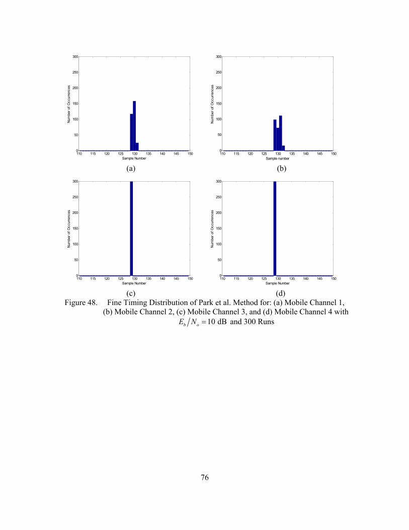
76

110 115 120 125 130 135 140 145 1500

50

100

150

200

250

300

Sample Number

Num

ber o

f Occ

urre

nces

110 115 120 125 130 135 140 145 1500

50

100

150

200

250

300

Sample number

Num

ber o

f Occ

urre

nces

(a) (b)

110 115 120 125 130 135 140 145 1500

50

100

150

200

250

300

Sample Number

Num

ber o

f Occ

urre

nces

110 115 120 125 130 135 140 145 1500

50

100

150

200

250

300

Sample Number

Num

ber o

f Occ

urre

nces

(c) (d)

Figure 48. Fine Timing Distribution of Park et al. Method for: (a) Mobile Channel 1, (b) Mobile Channel 2, (c) Mobile Channel 3, and (d) Mobile Channel 4 with

10 dBb oE N = and 300 Runs

77

4. Wang et al. Method This method consists of two steps as mentioned in Chapter III. The result of the

fine timing is based on the coarse timing algorithm. Here, we present the results for both

coarse and fine timing.

Figure 49 illustrates the coarse timing metric for different channels with different

values of b oE N . The negative values in the plots, which occur due to a subtraction op-

eration in the algorithm, do not affect the process. In this simulation, we expect the peak

to occur around sample number 113, i.e., the starting point of the 8th short symbol. It is

clear from Figure 49 that AWGN adversely affects the coarse timing metric. However,

since this algorithm is used for coarse timing, the accuracy is not important. We look for

a reference point to start the FFT operation for long symbols in the preamble of IEEE

802.11a. The CP of long symbols has 32 points, which gives a large interval to start the

FFT operation. In order to recover the long symbol, we can start the FFT window at any

point within the CP of long symbols.

Figure 50 shows the peak magnitude degradation plots for different channels with

different values of b oE N . For this method, peak degradation does not pose a problem for

values of b oE N over 10 dB.

78

0 20 40 60 80 100 120 140 160-0.4

-0.2

0

0.2

0.4

0.6

0.8

1

Sample Number

Tim

ing

Met

ric

Eb/No1=7.5Eb/No2=10Eb/No3=15Eb/No4=25

0 20 40 60 80 100 120 140 160-0.8

-0.6

-0.4

-0.2

0

0.2

0.4

0.6

0.8

Sample Number

Tim

ing

Met

ric

Eb/No1=7.5Eb/No2=10Eb/No3=15Eb/No4=25

(a) (b)

0 20 40 60 80 100 120 140 160-0.8

-0.6

-0.4

-0.2

0

0.2

0.4

0.6

0.8

1

Sample Number

Tim

ing

Met

ric

Eb/No1=7.5Eb/No2=10Eb/No3=15Eb/No4=25

0 20 40 60 80 100 120 140 160-0.2

-0.1

0

0.1

0.2

0.3

0.4

0.5

0.6

0.7

0.8

Sample Number

Tim

ing

Met

ric

Eb/No1=7.5Eb/No2=10Eb/No3=15Eb/No4=25

(c) (d)

0 20 40 60 80 100 120 140 160-0.4

-0.2

0

0.2

0.4

0.6

0.8

1

Sample Number

Tim

ing

Met

ric

Eb/No1=7.5Eb/No2=10Eb/No3=15Eb/No4=25

(e)

Figure 49. Wang et al. Method for Coarse Timing for: (a) AWGN Channel, (b) Mobile Channel 1, (c) Mobile Channel 2, (d) Mobile Channel 3, and (e) Mobile

Channel 4

79

-5 0 5 10 15 20

10-0 . 4

10-0 . 3

10-0 . 2

10-0 . 1

100

E b/N o

Pea

k M

agni

tude

A W G N c hanne lM ob. (Indoor) C h 1M ob. (Indoor) C h 2M ob. (O u tdoor) C h 3M ob. (O u tdoor) C h 4

Figure 50. Peak Magnitude Degradation of the Wang et al. Method for Coarse Timing

Figure 51 presents the fine timing distributions for the different channels. From

Figure 51, we observe that the timing variance is quite large. It even approaches that of

Schmidl and Cox Method in [8]. It spans 5 to 6 samples, which is the most that the IEEE

802.11a systems can tolerate since the channel impulse response of the IEEE 802.11a en-

vironment spans 10 samples [10]. In order to avoid ICI and ISI, the timing estimate

should lie somewhere within CP minus the length of channel impulse response.

As mentioned earlier in this section, for coarse timing, we have a large window.

But this could also affect the performance of the fine timing since it is based on the en-

ergy of the channel impulse response. This point actually raises some questions about this

method since the channel impulse response is not fixed for an environment. The magni-

tudes of the taps may not show a descending pattern, that is, the second or third tap may

be larger than the first one. In this case the optimum timing will change accordingly.

Another drawback is that this method employs the whole preamble of IEEE

802.11a, which is 16-µs long, whereas the other methods discussed earlier employ train-

ing symbols as short as 4 µs .

80

160 170 180 190 200 210 2200

50

100

150

200

250

300

Sample Number

Num

ber o

f Occ

urre

nces

160 170 180 190 200 210 2200

50

100

150

200

250

300

Sample Number

Num

ber o

f Occ

urre

nces

(a) (b)

160 170 180 190 200 210 2200

50

100

150

200

250

300

Sample Number

Num

ber o

f Occ

urre

nces

160 170 180 190 200 210 2200

50

100

150

200

250

300

Sample Number

Num

ber o

f Occ

urre

nces

(c) (d)

Figure 51. Fine Timing Distribution of Wang et al. Method for: (a) Mobile Channel 1, (b) Mobile Channel 2, (c) Mobile Channel 3, and (d) Mobile Channel 4 with

10 dBb oE N = and 300 Runs

81

5. Proposed Method 1 (a Modification of the Park et al. Method) We proposed this method as a modification to Park et al.’s method to improve the

performance of the timing metric in AWGN. Figure 52 presents the timing metric for dif-

ferent channel models with different values of b oE N . The four plots for different values

of b oE N in Figure 52 are nearly the same. This result indicates that this method

achieved the goal of robustness under AWGN. Despite its robustness under the AWGN

and the outdoor channels, like the Park et al. method, this method performs poorly under

indoor channels due to its sensitivity to multi-path channels. The timing metrics for out-

door channels are close to those under ideal conditions (see Figure 26).

82

80 90 100 110 120 130 140 1500

0.2

0.4

0.6

0.8

1

Sample Number

Tim

ing

Met

ric

Eb/No1=7.5Eb/No2=10Eb/No3=15Eb/No4=25

90 100 110 120 130 140 150 1600

0.1

0.2

0.3

0.4

0.5

0.6

0.7

0.8

0.9

1

Sample Number

Tim

ing

Met

ric

EbNo1=7.5EbNo2=10EbNo3=15EbNo4=25

(a) (b)

90 100 110 120 130 140 150 1600

0.1

0.2

0.3

0.4

0.5

0.6

0.7

0.8

0.9

1

Sample Number

Tim

ing

Met

ric

Eb/No1=7.5Eb/No2=10Eb/No3=15Eb/No4=25

80 90 100 110 120 130 140 1500

0.1

0.2

0.3

0.4

0.5

0.6

0.7

0.8

0.9

1

Sample Number

Tim

ing

Met

ric

Eb/No1=7.5Eb/No2=10Eb/No3=15Eb/No4=25

(c) (d)

80 90 100 110 120 130 140 1500

0.2

0.4

0.6

0.8

1

Sample Number

Tim

ing

Met

ric

Eb/No1=7.5Eb/No2=10Eb/No3=15Eb/No4=25

(e)

Figure 52. Proposed Method 1 for: (a) AWGN Channel, (b) Mobile Channel 1, (c) Mo-bile Channel 2, (d) Mobile Channel 3, and (e) Mobile Channel 4

83

Figure 53 shows the peak magnitude degradation for different channels. The im-

provement in the peak magnitude is apparent in this method when compared to that of the

Park et al. method (see Figure 47).

-5 0 5 10 15 20

10-0 . 3

10-0 . 2

10-0 . 1

100

100 . 1

E b/N o

Pea

k M

agni

tude

A W G N c hanne lM ob .(Indoor) C h 1M ob.(Indoor) C h 2M ob.(O u tdoor) C h 3M ob.(O u tdoor) C h 4

Figure 53. Peak Magnitude Degradation of the Proposed Method 1

Figure 54 shows the fine timing distribution for Proposed Method 1. The starting

point of the OFDM symbol in this simulation is 128. Despite the relatively poor perform-

ance displayed for indoor channels, this method performs well for the outdoor channels.

The timing estimate for outdoor channels in Figures 54(c) and 54(d) is the true timing

point. In general, the performance of the Proposed Method 1 is comparable to that of the

Park et al. method in indoor channels. In fact, considering the peak degradation and ro-

bustness under AWGN, Proposed Method 1 outperforms the Park et al. Method in indoor

channels.

84

110 115 120 125 130 135 140 145 150 155 1600

50

100

150

200

250

300

Sample Number

Num

ber o

f Occ

urre

nces

110 115 120 125 130 135 140 145 150 155 1600

50

100

150

200

250

300

Sample Number

Num

ber o

f Occ

urre

nces

(a) (b)

110 115 120 125 130 135 140 145 150 155 1600

50

100

150

200

250

300

Sample Number

Num

ber o

f Occ

urre

nces

110 115 120 125 130 135 140 145 150 155 1600

50

100

150

200

250

300

Sample Number

Num

ber o

f Occ

urre

nces

(c) (d)

Figure 54. Fine Timing Distribution of Proposed Method 1 for: (a) Mobile Channel 1, (b) Mobile Channel 2, (c) Mobile Channel 3, and (d) Mobile Channel 4 with

10 dBb oE N = and 300 Runs

85

6. Proposed Method 2 In this method our motivation was to achieve the fine timing in a shorter time and

to use the cross-correlation instead of auto-correlation. However, we also know that the

energy contained in the training symbol is not the only concern. The shorter the symbol

becomes, the more the channel and AWGN affect its performance. Besides, this means

that more power per sample is required to keep the same energy level. For a 16-sample

PN sequence whose values are taken from QPSK constellation, it can be shown that the

transmitter requires 10 dB more power per sample than that for the data symbols.

We first simulated the PN sequence with 16 points taken from Table 8 as de-

scribed in Section C of Chapter III. The plots for timing metric are shown in Figure 55. It

can be seen that the timing metric has one main lobe and no other side lobes. The per-

formance for indoor channels and outdoor channels is similar. This method performs

well with AWGN as well.

Figure 56 displays the fine timing distribution plots for each channel. Figure 57

presents the peak magnitude degradation plot. Examining the results in Figures 55 to 57,

this method yields desirable performance in three ways:

• It performs well for indoor environments. This is very important since it is where the most degradation is observed in other methods.

• It is robust with AWGN. We observed that AWGN does not affect the timing metric much.

• Large delays and high mobility do not affect the timing.

Basically, some of the results, such as robustness with AWGN, were expected.

Since we use a cross-correlation-based technique rather than an auto-correlation-based

technique, it is obvious that the influence of noise will be diminished. In [39], it was

shown that the cross-correlation-based techniques outperform the auto-correlation-based

techniques.

86

0 50 100 150 200 250 300 3500

10

20

30

40

50

60

70

80

90

100

Sample Number

Tim

ing

Met

ric

Eb/No1=7.5Eb/No2=10Eb/No3=15Eb/No4=25

0 50 100 150 200 250 300 3500

10

20

30

40

50

60

70

80

90

100

Sample Number

Tim

ing

Met

ric

Eb/No1=7.5Eb/No2=10Eb/No3=15Eb/No4=25

(a) (b)

0 50 100 150 200 250 300 3500

20

40

60

80

100

120

140

Sample Number

Tim

ing

Met

ric

Eb/No1=7.5Eb/No2=10Eb/No3=15Eb/No4=25

0 50 100 150 200 250 300 3500

20

40

60

80

100

120

140

160

180

Sample Number

Tim

ing

Met

ric

Eb/No1=7.5Eb/No2=10Eb/No3=15Eb/No4=25

(c) (d)

Figure 55. Proposed Method with 16-sample PN Sequence for: (a) Mobile Channel 1, (b) Mobile Channel 2, (c) Mobile Channel 3, and (d) Under Mobile Chan-

nel 4

87

80 100 120 140 160 180 2000

50

100

150

200

250

300

350

400

Sample Number

Num

ber o

f Occ

urre

nces

80 100 120 140 160 180 2000

50

100

150

200

250

300

350

400

Sample Number

Num

ber o

f Occ

urre

nces

(a) (b)

80 100 120 140 160 180 2000

100

200

300

400

500

600

Sample Number

Num

ber o

f Occ

urre

nces

80 100 120 140 160 180 2000

100

200

300

400

500

600

Sample Number

Num

ber o

f Occ

urre

nces

(c) (d)

Figure 56. Fine Timing Distribution of Proposed Method 2 for: (a) Mobile Channel 1, (b) Mobile Channel 2, (c) Mobile Channel 3, and (d) Mobile Channel 4 with

10 dBb oE N = 600 Runs

88

-5 0 5 10 15 2010

1

102

103

E b/N o

Pea

k M

agni

tude

A W G N c hanne lIndoor C h= 21Indoor C h= 22O utdoor C h= 23O utdoor C h= 24

Figure 57. Peak Magnitude Degradation of the Proposed Method 2 with 16-sample PN

Sequence

We also ran simulations with 8-sample PN sequences that contain the same en-

ergy as longer sequences. The timing metric plots, the peak degradation plots and the fine

distribution plot for Mobile Channel 2 are presented in Figure 58. Based on these, the re-

sults for the 8-point PN sequence are comparable to the results for the16-sample scheme.

However, these results may be misleading since the PN sequences have the same energy.

Preserving energy while shortening the training sequence means that the transmitter has

to use more power in order to keep the same energy level for fewer number of samples.

This is not practical because of the system power limitations. Another drawback is that

the performance of this scheme may degrade under sudden changes in noise due to its

shortness.

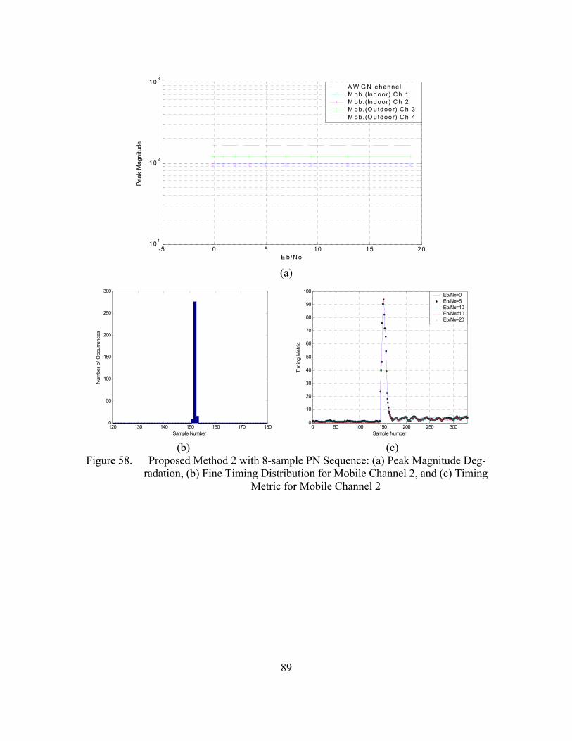
89

-5 0 5 10 15 2010

1

102

103

E b/N o

Pea

k M

agni

tude

A W G N c hanne lM ob. (Indoor) C h 1M ob. (Indoor) C h 2M ob. (O utdoor) C h 3M ob. (O utdoor) C h 4

(a)

120 130 140 150 160 170 1800

50

100

150

200

250

300

Sample Number

Num

ber o

f Occ

urre

nces

0 50 100 150 200 250 3000

10

20

30

40

50

60

70

80

90

100

Sample Number

Tim

ing

Met

ricEb/No=0Eb/No=5Eb/No=10Eb/No=10Eb/No=20

(b) (c)

Figure 58. Proposed Method 2 with 8-sample PN Sequence: (a) Peak Magnitude Deg-radation, (b) Fine Timing Distribution for Mobile Channel 2, and (c) Timing

Metric for Mobile Channel 2

90

7. Comparison of the Timing Methods We present two tables summarizing the results of the simulations. Table 16 evalu-

ates the methods in terms of different channel conditions and ease of implementation.

The evaluations are inferred from the simulations results. The values in Table 17 are the

timing offset in terms of number of samples showing the width of the fine timing distri-

bution of a method for a given channel type.

robustrobustrobustfairly good6. Proposed 2

goodrobustrobustpoor5. Proposed 1

poorpoorgoodpoor4. Wang et al.

goodpoorfairly goodgood3. Park et al.

poorgoodgoodgood2. Minn and Bhargava

poorpoorgoodpoor1. Schmidl and Cox

ImplementationAWGNOutdoorIndoor

Method

Condition

robustrobustrobustfairly good6. Proposed 2

goodrobustrobustpoor5. Proposed 1

poorpoorgoodpoor4. Wang et al.

goodpoorfairly goodgood3. Park et al.

poorgoodgoodgood2. Minn and Bhargava

poorpoorgoodpoor1. Schmidl and Cox

ImplementationAWGNOutdoorIndoor

Method

Condition

Table 16. Performance Evaluation of Timing Methods

91

11226. Proposed 2*

11435. Proposed 1

44664. Wang et al.

11433. Park et al.

21432. Minn and Bhargava

32871. Schmidl and Cox

Mobile OutdoorChannel 4

Mobile OutdoorChannel 3

Mobile IndoorChannel 2

Mobile IndoorChannel 1

Method

Channel

11226. Proposed 2*

11435. Proposed 1

44664. Wang et al.

11433. Park et al.

21432. Minn and Bhargava

32871. Schmidl and Cox

Mobile OutdoorChannel 4

Mobile OutdoorChannel 3

Mobile IndoorChannel 2

Mobile IndoorChannel 1

Method

Channel

Table 17. Fine Timing Offset in Samples (* indicates the results for 16-point

PN sequence)

For the Schmidl and Cox method, we discovered that the plateau inherent in the

method raises uncertainty in the timing distribution. The timing distribution may span as

many as 8 samples, as can be seen in Table 17. The edge of the timing metric plateau

changes depending on the multi-path, noise power, and delays, which makes the imple-

mentation very difficult. Another disadvantage is the question of finding the optimum

timing point. However, there are other studies showing some advantages of this method.

For example, [21] shows that Schmidl and Cox method is very robust against carrier fre-

quency offset and fading.

The Minn and Bhargava method successfully avoids the disadvantages of the

Schmidl and Cox method. It does not have a plateau, and the variance of the estimator is

lower. Nevertheless, in order to reach this conclusion, we assumed that the middle peak

always has larger amount of energy than the other peaks on both sides.

The main disadvantage that we noted about the Park et al. method is that it is very

sensitive to AWGN. However, it is worth noting that, while the normalized metric value

92

drops below 0.4, the peaks due to correlation with noise and data sent after the training

symbol do not quickly go up. This improves the performance of the method. For rela-

tively high values of b oE N , this method is robust in outdoor channels whereas the tim-

ing distribution has a tendency to worsen in indoor channels.

The Wang et al. method has the second largest timing estimator variance after the

Schmidl and Cox method. Another drawback to this method is that it uses the

whole16-µs preamble of the IEEE 802.11a to obtain a timing estimate.

The performance of the Proposed Method 1 is comparable to that of the Park et

al. method. It outperforms the Park et al. method in terms of peak degradation and sensi-

tivity to AWGN; it performs well under low values of b oE N . Besides, its performance

is robust under outdoor channels.

Proposed Method 2 is based on cross-correlation rather than auto-correlation. It

exhibited the best performance overall, that is, it is highly reliable and robust under out-

door channels while its performance under indoor channels is comparable to that of other

methods.

One observation regarding the channel effects is that the timing methods in gen-

eral performed poorly under multipath. The indoor channels were characterized by

Rayleigh distribution and 18 paths [12] whereas the outdoor channels had 6 paths with a

Rician factor of 0.5. Other characteristics of the channels, such as a time-varying nature,

delay spread profile and mobility, do not affect the timing greatly. Another important ob-

servation we made is that larger delays do not affect timing synchronization. Mobile

Channel 4, with the most severe conditions, has the highest BER among the all channels

for 10 dBb oE N = . Despite having the highest BER, this channel provided better results

in terms of timing synchronization. This is because all of the timing methods we studied

are based on the energy of the training signal. The algorithms work with the first arriving

path, and in the case of large delays, the first received symbol is less likely to be affected

by its delayed versions.

93

Overall, the Proposed Method 2 performed better than others for indoor channels,

and the Park et al. method, the Proposed Method 1 and the Proposed Method 2 worked

well for outdoor channels.

D. SUMMARY In this chapter we tested the timing methods of interest for different channels. We

ran simulations for each method under all the channel models. We presented and dis-

cussed the simulation results. In the next chapter, we present a summary of the work done

in this thesis, outline significant results and provide suggestions for future studies.

94

THIS PAGE INTENTIONALLY LEFT BLANK

95

V. CONCLUSION

The objective of this thesis was to investigate the need for timing synchronization,

the effects of timing errors, and the performance of various timing methods under mobile

indoor and outdoor channel conditions. The objective was accomplished by investigating

the effects of timing errors on OFDM systems and the performances of six timing meth-

ods through a series of simulations.

A. SUMMARY OF THE WORK DONE In this thesis, we first introduced the basics of OFDM, an OFDM-based system

model, and two OFDM-based standards, namely the IEEE 802.11a and IEEE 802.16a

standards. The need for timing synchronization in OFDM systems and the effects of tim-

ing errors were investigated. Six different timing methods were introduced

A Matlab simulation of an OFDM system was developed, and the timing methods

were simulated for four mobile channels. Two indoor and two outdoor channel models

were used. The performance of the timing methods was studied for all of the channel

models by observing the timing metric and the timing distributions. Finally a perform-

ance comparison of the methods was provided.

B. SIGNIFICANT RESULTS AND CONCLUSIONS The results of the timing methods allowed us to determine which method per-

forms better under which channel conditions. In general, all of the methods exhibited sat-

isfactory performance for outdoor channels. The Park et al. method and the Proposed

Method 1 performed well for indoor channels. The Proposed Method 2, a cross-

correlation based method, showed a robust and satisfactory performance for both indoor

and outdoor channels.

The timing algorithms are sensitive to multi-path. The timing methods displayed a

robust performance for Mobile Channel 4, which has the highest BER for

10 dB.b oE N = This result indicates that large delays do not affect the timing algo-

rithms.

96

The Schmidl and Cox method and the Minn and Bhargava method have signifi-

cant implementation drawbacks that hinder their usage for reliable timing synchroniza-

tion purposes.

C. SUGGESTIONS FOR FUTURE STUDIES The OFDM communication system used in this thesis was simulated by using a

base-band model. A detailed radio frequency implementation may be undertaken in a fu-

ture study to observe the performance of the methods in a more realistic environment.

The system used in this thesis was based on the OFDM-based IEEE 802.11a stan-

dard, used for wireless local area networks. There are other OFDM-based standards, such

as wireless metropolitan area networks standards of IEEE 802.16a and IEEE.16e (in pro-

gress). These systems have different OFDM parameters compared to the parameters used

in this thesis. The required conditions to have the correct timing would be different for

these standards, also the amount of ISI and ICI would differ. The performance of timing

methods may be investigated for a model based on the IEEE 802.16a standard in a future

effort.

Only timing synchronization techniques were studied in this thesis, which implies

that frequency synchronization was realized by another process using the same training

sequence or a different sequence depending on the frequency synchronization technique

used. There are some synchronization techniques that realize both timing and frequency

synchronization by employing the same training sequence [43]. The performance of such

techniques may be studied under the same conditions as in this work.

97

APPENDIX A. MATLAB CODE

In this appendix, the Matlab code used in the simulations is presented.

%AWGN %------------------------------------------------------------------------------------- %Title : Additive White Gaussian Noise %Author : Prof. Paul H. Moose, Naval Postgraduate School %Modified by : Ahmet Yasin ERDOGAN, Naval Postgraduate School %-------------------------------------------------------------------------------------- %INPUTS : % X : Time domain samples of the transmitted signal % s : Seed parameter % sigma : AWGN Noise variance parameter for calculating Eb/No % %OUTPUTS: % Y : Time domain samples of the transmitted signal plus AWGN %--------------------------------------------------------------------------------------- function Y = awgn(X,sigma,s) % %Find dimensions of the input array [rr,cc]=size(X); % randn('seed',s+30); %Generate a random real part wreal=randn(rr,cc); %Generate a random imaginary part randn('seed',s+40); wimg=i*randn(rr,cc); % %An array of random complex entries chosen from a normal distribution with %mean 0.0 and variance 1.0. Array dimensions are the same as X. W=wreal+wimg; % %Random noise multiplied by the sigma factor and added to the signal. Y=X+(sigma.*W);

98

%BIN2DECI %------------------------------------------------------------------------------------- % %Title : Binary To Decimal Conversion %Author : Tan Kok Chye, Naval Postgraduate School %-------------------------------------------------------------------------------------- %INPUT : % v_x : Binary input % %OUTPUT: % v_y : Decimal output %--------------------------------------------------------------------------------------- function v_y=bin2deci(v_x) v_l=length(v_x); v_y=(v_l-1:-1:0); v_y=2.^v_y; v_y=v_x*v_y';

99

%BM %------------------------------------------------------------------------------------- % %Title : Binary to M-ary Converter %Author : Prof. Paul H. Moose, Naval Postgraduate School %Modified by : Ahmet Yasin ERDOGAN, Naval Postgraduate School % %-------------------------------------------------------------------------------------- %INPUTS: % q : Base 2 exponent for M-ary symbol generation % v : Binary data vector % %OUTPUTS: % m : M-ary output vector in decimal notation %--------------------------------------------------------------------------------------- function m=bm(q,v) % %Find the length of input vector,v,and determine if there is a remainder %after dividing by q n=length(v); r=rem(n,q); % %If there is no remainder,don't pad v input vector. Otherwise add the appropriate %number of zeros to generate a code word with an exact multiple of q bits. % if r==0 v=v; else v=[v zeros(1,q-r)]; end % %Place least significant bit of the symbol on the left end. map=1; for j=1:q-1 map=[map 2^j]; end % %Remove q bits at a time from v to generate m-ary symbol values. n=length(v); p=round(n/q); A=zeros(q,p); A(:)=v; m=map*A; m_ary_msg=m;

100

%CDLDLV %------------------------------------------------------------------------------------- % %Title : CDL Block Deinterleaver %Author : Prof. Paul H. Moose, Naval Postgraduate School %Modified by : Ahmet Yasin ERDOGAN, Naval Postgraduate School % %-------------------------------------------------------------------------------------- %INPUTS: % l : Intermediate matrix row number % k : Intermediate matrix column number % dcase: Indicates the deinterleaving method to be % used (9 different cases). In our thesis only block interleaving was used. % si : Input message string to be deinterleaved % SYNC : Frame synchronization bits (Not used in COFDM simulation) % %OUTPUTS: % s : Interleaved output string %--------------------------------------------------------------------------------------- function s=cdldlv(l,k,dcase,si,SYNC) si(length(si)+l-length(SYNC):length(si))=zeros(l,length(SYNC)); N=length(si); if l*k==N x=zeros(l,k); x(:)=si; K=(1:k)-1; CR=K.*(K+1)/2; L=(1:l)-1; RR=L.*(L+1)/2; % if dcase==1 for kk=1:k x(:,kk)=rotm(x(:,kk),CR(kk)); end elseif dcase==2 for kk=1:k [z,x(:,kk)]=rotm(x(:,kk),CR(kk)); end elseif dcase==3 for kk=1:l x(kk,:)=rotm(x(kk,:),RR(kk)); end elseif dcase==4 for kk=1:l [z,x(kk,:)]=rotm(x(kk,:),RR(kk));

101

end elseif dcase==5 for kk=1:k x(:,kk)=rotm(x(:,kk),CR(kk)); end for ll=1:l x(ll,:)=rotm(x(ll,:),RR(ll)); end elseif dcase==6 for kk=1:k [z,x(:,kk)]=rotm(x(:,kk),CR(kk)); end for ll=1:l x(ll,:)=rotm(x(ll,:),RR(ll)); end elseif dcase==7 for kk=1:k x(:,kk)=rotm(x(:,kk),CR(kk)); end for ll=1:l [z,x(ll,:)]=rotm(x(ll,:),RR(ll)); end elseif dcase==8 for kk=1:k [z,x(:,kk)]=rotm(x(:,kk),CR(kk)); end for ll=1:l [z,x(ll,:)]=rotm(x(ll,:),RR(ll)); end end x=x'; s=x(:); s=s'; end

102

%CDLILV %------------------------------------------------------------------------------------- % %Title : CDL Block Interleaver %Author : Prof. Paul H. Moose, Naval Postgraduate School %Modified by : Ahmet Yasin ERDOGAN, Naval Postgraduate School % %-------------------------------------------------------------------------------------- %INPUTS: % l : Intermediate matrix row number % k : Intermediate matrix column number % dcase: Indicates the deinterleaving method to be % used (9 different cases). In our thesis only block interleaving was used. % si : Input message string to be deinterleaved % SYNC : Frame synchronization bits (Not used in COFDM simulation) % %OUTPUTS: % si : Interleaved output string % %Subroutines Used : rotm.m %--------------------------------------------------------------------------------------- function si = cdlilv(l,k,dcase,s,SYNC) N=length(s); if l*k==N x=zeros(l,k); x=x'; x(:)=s; x=x'; Intermediate_mx=x; K=(1:k)-1; CR=K.*(K+1)/2; L=(1:l)-1; RR=L.*(L+1)/2; % if dcase==1 for kk=1:k [z,x(:,kk)]=rotm(x(:,kk),CR(kk)); end elseif dcase==2 for kk=1:k x(:,kk)=rotm(x(:,kk),CR(kk)); end elseif dcase==3 for kk=1:l [z,x(kk,:)]=rotm(x(kk,:),RR(kk));

103

end elseif dcase==4 for kk=1:l x(kk,:)=rotm(x(kk,:),RR(kk)); end elseif dcase==5 for ll=1:l [z,x(ll,:)]=rotm(x(ll,:),RR(ll)); end for kk=1:k [z,x(:,kk)]=rotm(x(:,kk),CR(kk)); end elseif dcase==6 for ll=1:l [z,x(ll,:)]=rotm(x(ll,:),RR(ll)); end for kk=1:k x(:,kk)=rotm(x(:,kk),CR(kk)); end elseif dcase==7 for ll=1:l x(ll,:)=rotm(x(ll,:),RR(ll)); end for kk=1:k [z,x(:,kk)]=rotm(x(:,kk),CR(kk)); end elseif dcase==8 for ll=1:l x(ll,:)=rotm(x(ll,:),RR(ll)); end for kk=1:k x(:,kk)=rotm(x(:,kk),CR(kk)); end end x; si=x(:); si=si'; end si(length(si)-length(SYNC)+1:length(si))=SYNC;

104

%CDRCDLFT %------------------------------------------------------------------------------------- % %Title : COFDM Encoder with CDL Interleaver %Author : Prof. Paul H. Moose, Naval Postgraduate School %Modified by : Ahmet Yasin ERDOGAN, Naval Postgraduate School % %-------------------------------------------------------------------------------------- %INPUTS: % pic : Parameter indicating the figure number % s : Seed parameter % freqno : Number of OFDM frequencies (sub-carriers) used in each message array % rintlv : Parameter for intermediate matrix row number % cintlv : Parameter for intermediate matrix column number % N : Number of FFT frequency sample points,must be larger than freqno % mary : Initial M-ary symbol format (OFDM symbol bit length) % nary : Final N-ary symbol format (PSK symbol bit length) % fort : Selects either frequency (fort=1) or time (fort=0) differential encoding % %OUTPUTS: % Fa : Frequency array of prearranged modulation values % MD : Matrix of differentially encoded complex values %(unity magnitude and one of N-ary possible phases (N-PSK)) % B : Matrix of 8-ary symbols % nsymno: Number of N-ary generated symbols % %Subroutines Used : marymsg.m,cdlilv.m,mb.m,bm.m,difcdrft.m,cmv2fa.m %--------------------------------------------------------------------------------------- func-tion[Fa,MD,B_ce,B_random,nsymno]=cdrcdlft(pic,dcase,s,freqno,rintlv,cintlv,N,mary,nary,fort); % % Determine whether the number of OFDM frequencies are even, indicated % by the "freqno" parameter. If odd, go to error message. Odd frequencies are not al-lowed % since the formation of the frequency array is symmetrical and even. % if rem(freqno,2)~=0 disp('ERROR: The number of matrix columns, representing OFDM frequencies, must be an even number!') elseif rem(freqno,2)==0 % % Check if interleaver matrix dimensions are greater than freqno. % If not, then display error message and stop. %

105

if (rintlv*cintlv)<(freqno) disp('') disp('ERROR: The row and column interleave parameters are not compatible with # of OFDM frequencies!') disp('') else % Calculate the row symbol number symno=rintlv*cintlv/freqno; % % Display error message if symno and freqno not compatible with rintlv and cintlv and stop. % If not compatible,the interleaver function does not work correctly. % if rem(symno,1)~=0 disp('') disp('ERROR: The row and column interleave parameters are not compatible with # of OFDM frequencies!') disp(' For the entered rintlv, cintlv, and freqno parameters, the calculated symno is:') disp(symno) multiesall=mltpl(rintlv,cintlv); multies=multiesall(1,(2:length(multiesall)-1)); disp(' Possible choices for freqno based upon rintlv and cintlv are:') disp('') disp(multies) elseif rem(symno,1)==0 if freqno >= N; disp('') disp('ERROR: The number of frequency points, N, needs to be increased !') disp('N must be larger than:') disp('') disp(freqno) disp('') elseif freqno < N; % % Generate a random message matrix of m-ary symbols,based upon parameter,mary. Nmbr_of_symbols =symno*freqno; [B_ce,B_random]=marymsg(mary,symno,freqno); Rndm_m_ary_msg=B_random; % % Perform a block interleaving function on the matrix, B, with rintlv rows % and cintlv columns. SYNC=[]; [Br Bc]=size(B_ce); Bt=B_ce'; Bvect=Bt(:)';

106

si=cdlilv(rintlv,cintlv,dcase,Bvect,SYNC); Bi=reshape(si,Bc,Br)'; Intrlvd_array=Bi; m1=bm(nary,mb(mary,Bi)); lengthm1=length(m1); nsymno=lengthm1; remm1=rem(lengthm1,freqno); if remm1==0; m1=m1; else zero=zeros(freqno-remm1); m1=[m1 zero(1,:)]; end length2m1=length(m1); m=(reshape(m1,freqno,length2m1/freqno))'; N_ary_msg=m; % % Generate a differentially encoded matrix of complex % values with unity magnitude and one of (2^n) equal phases. MDD=difcdrft(nary,m,fort); [MDm MDn]=size(MDD); MD=MDD; Cmplx_mod_array=MDD; % % Form the frequency array of modulation values that include guard interval. Fa=cmv2fa(N,MD); Freq_array=Fa; end end end end

107

%CHANCDL %------------------------------------------------------------------------------------- % %Title : Simulations for AWGN & Multipath Fading Channel %Author : Dave Roderick, Naval Postgraduate School %Modified By :Ersoy OZ, Naval Postgraduate School %-------------------------------------------------------------------------------------- %Subroutines Used : cdrcdlft.m,tda.m,awgn.m,chuhf.m,itda.m,decdrcdl.m,check.m %--------------------------------------------------------------------------------------- function chancdl(chnmdl,wait,pic,dcase,s,freqno,rintlv,cintlv,N,mary,nary,n,k,blklgth,Ng,sigs,loss,dly,dop,freqspace,fort) sigvect=sigs; klgth=length(k); chklp=1; symno=rintlv*cintlv/freqno; errvect=[]; bervect=[]; freqerrmx=[]; errsperpr=[]; Es_No=[]; Eb_No=[]; sermx=[]; bermx=[]; rowerrmx=[]; for lp=1:length(sigvect); [xmt,modvals,B_ce,B_random,nsymno]=cdrcdlft(pic,dcase,s,freqno,rintlv,cintlv,N,mary,nary,fort); xmtifft=tda(Ng,xmt); xmtpts=1:length(xmtifft); if chnmdl==0 sandn=xmtifft; elseif chnmdl==1 disp(['Sigma=',num2str(sigvect(lp))]); sandn=awgn(xmtifft,sigvect(lp),s); elseif chnmdl==21 sandmltpth=chuhf(s+1,xmtifft,loss,dly,dop,N,freqspace); disp(['Sigma=',num2str(sigvect(lp))]);

108

sandn=awgn(sandmltpth,sigvect(lp),s); elseif chnmdl==22 sandmltpth=chuhf(s+1,xmtifft,loss,dly,dop,N,freqspace); disp(['Sigma=',num2str(sigvect(lp))]); sandn=awgn(sandmltpth,sigvect(lp),s); elseif chnmdl==23 disp(['Sigma=',num2str(sigvect(lp))]); sandmltpth=channel_a(xmtifft); sandn=awgn(sandmltpth,sigvect(lp),s); elseif chnmdl==24 disp(['Sigma=',num2str(sigvect(lp))]); sandmltpth=channel_b(xmtifft); sandn=awgn(sandmltpth,sigvect(lp),s); end [sandnfft,Md]=itda(Ng,sandn,sigvect(lp),lp);% sigvect added K=(length(modvals(1,:)))/2; [rcvd,rcvd_bit,random_msg,random_bit,M,MM]=decdrcdl(pic,dcase,K,sandnfft,nsymno,freqno,rintlv,cintlv,mary,nary,fort,B_random); %%Transmitted_msg=B_random; Transmitted_msg=random_msg; Received_msg=rcvd; [er-rors,bit_error,freqerrs,errmx,rowerrs]=check(pic,random_msg,random_bit,rcvd,rcvd_bit,n,k(chklp),blklgth); errvect=[errvect,errors]; bervect=[bervect,bit_error]; freqerrmx=[freqerrmx;freqerrs]; rowerrmx=[rowerrmx;rowerrs]; crntEs_No=1/(2*N*(sigvect(lp)^2)); crntEb_No=crntEs_No; % %based on M=4 i.e. for coded QPSK, Eb=Es. Es_No=[Es_No,crntEs_No]; Eb_No=[Eb_No,crntEb_No]; Es_Nodb=10*log10(Es_No); Eb_Nodb=10*log10(Eb_No); metric(lp,:)=Md; end

109

%Plotting the metric %----------------------------------------------------------------------------------------- figure(33); plot(metric(1,:)); xlabel('Sample Number'); ylabel('Timing Metric'); title('Park e.t Method'); axis([0 160 0 1]); hold on plot(metric(2,:),'r.'); hold on plot(metric(3,:),'c+'); hold on plot(metric(4,:),'m'); gtext(['Channel model=',num2str(chnmdl)]); grid; %text(0,0,['Eb_No=',num2str(Eb_No)]); leg-end(['EbNo1=',num2str(Eb_Nodb(1))],['EbNo2=',num2str(Eb_Nodb(2))],['EbNo3=',num2str(Eb_Nodb(3))],['EbNo4=',num2str(Eb_Nodb(4))]); %----------------------------------------------------------------------------------------------- % ser=errvect/(symno*freqno); ber=bervect/(2*symno*freqno); sermx=[sermx;ser]; bermx=[bermx;ber]; errsum=sum(errvect); errsperpr=[errsperpr,errsum]; errmax=max(rowerrmx'); % % PLOTS % figure(pic+1) plot(modvals,'*') hold on; plot(0,0,'+') hold off; %title(['Transmitted Signal Constellation',int2str(2^nary), '-ary (QPSK) ']) xlabel('Re'); ylabel('Im'); axis('square');orient tall;grid pause(wait); %%%%Plot of FFT POINTS%%%% %figure(pic+2)

110

%plot([0:N-1],abs(xmt),'*') %title(['Frequency Array Plot (number of FFT frequency points are ',int2str(N),')']) %xlabel(['Guard interval length is ',int2str(N-freqno)]) %axis('square');orient tall;grid %pause(wait); % figure(pic+2) surf(abs(modvals)); shading interp;grid;orient tall %title(['Magnitude Plot of Transmitted Signal']) xlabel('OFDM Subcarrier Number') ylabel('Symbol Row Number') zlabel('Signal Magnitude') pause(wait); % figure(pic+3) plot(M,'*');hold on; plot(0,0,'+');hold off; %title(['Received Signal Constellation', int2str(2^nary),'-ary (QPSK), (Before Differential Decoding)']) xlabel('Re'); ylabel('Im'); orient tall;axis('square');grid pause(wait); % figure(pic+4) plot(MM,'+') hold on; plot(0,0,'+') hold off; %title(['Received Signal Constellation',int2str(2^nary),'-ary (QPSK), (After Differential Decoding)']) xlabel('Re'); ylabel('Im'); orient tall;axis('square');grid pause(wait); % figure(pic+5) surf(abs(M)); shading interp grid;orient tall %title(['Magnitude Variation of Received Signal (Sigma=',num2str(sigvect(lp)),')']) xlabel('OFDM Subcarrier Number') ylabel('Symbol Row Number') zlabel('Signal Magnitude')

111

pause(wait); % if errsum~=0 %%%%PERFORMANCE PLOTS%%%% %theoretical on top of simulation curves %q=length(Eb_No) %for i=1:q %P=0.5*(erfc(Eb_No(1,i))*(1-0.25*erfc(Eb_No(1,i)))); %Pb(1,i)=P; %end figure(pic+6) %semilogy(Eb_Nodb,Pb,'m');grid;hold on; semilogy(Eb_Nodb,ber);hold on;grid if fort==1 %title('Performance curve: BER vs. Eb/No for QPSK Signaling (Freq. Diff.Enc.)') elseif fort==0 %title('Performance curve: BER vs. Eb/No for QPSK Signaling (Time. Diff.Enc.)') end xlabel('Eb/No(dB)'); ylabel('BER'); %legend('theorical curve','simulation curve');orient tall % figure(pic+7) %semilogy(Es_Nodb,2*Pb,'m');hold on semilogy(Es_Nodb,ser);grid;hold on if fort==1 %title('Performance curve: SER vs. Es/No (Freq. Diff.Enc.)') elseif fort==0 %title('Performance curve: SER vs. Es/No (Time. Diff.Enc.)') end xlabel('Es/No(dB)'); ylabel('SER'); %legend('theoretical curve','simulation curve');orient tall end %end

112

%channel_a %------------------------------------------------------------------------------------- % %Title : Mobile Channel 2 %Author : Prof.Roberto Cristi, Naval Postgraduate School %Modified By : Ahmet Yasin ERDOGAN, Naval Postgraduate School %-------------------------------------------------------------------------------------- %Subroutines Used : jakes.m %-------------------------------------------------------------------------------------- function yr=channel_a(xt) [asd asn]=size(xt); xt=xt.'; xt=xt(:).'; % % yr=channel(xt) % with xt=transmitted vector % yr=received vector % length(yr)=length(xt) % % if the program gives you an error, just increase the size of the % transmitted vector "xt" Fs=1.25*10^6; % sampling frequency (Hz) Fd=200; % doppler frequency (Hz) %Parameters for Channel A Td=[0.0, 0.25,0.5,1.0,1.9,2.2]; % time delays (in microsec) PdB=[0.0,-1.0,-9.0,-10.0,-15.0,-20.0]; % Powers (in dB) K=[0,0,0,0,0,0]; % Ricean Factor Td=Td*(10^(-6)); % time delays (in sec) nd=round(Td*Fs); % time delay in samples P=10.^(PdB/10); % Powers (Linear) Np=length(xt); yr=zeros(size(xt)); for k=1:length(Td) g=jakes(Fd, Fs, Np); s=sqrt(P(k)/(K(k)+1)); % random path m=sqrt(P(k)*K(k)/(K(k)+1)); % direct path total=s*g+m*exp(j*2*pi*Fd/Fs*(0:length(xt)-1)); yr=yr+[zeros(1,nd(k)), xt(1:length(xt)-nd(k))].*total; end yr=reshape(yr,asn,asd).';

113

%channel_b %------------------------------------------------------------------------------------- % %Title : Severe Mobile channel %Author : Prof.Roberto Cristi, Naval Postgraduate School %Modified By : Ahmet Yasin ERDOGAN, Naval Postgraduate School %-------------------------------------------------------------------------------------- %Subroutines Used : jakes.m %-------------------------------------------------------------------------------------- function yr=channel_b(xt) [asd asn]=size(xt); xt=xt.'; xt=xt(:).'; % % yr=channel(xt) % with xt=transmitted vector % yr=received vector % length(yr)=length(xt) % % if the program gives you an error, just increase the size of the % transmitted vector "xt" Fs=1.25*10^6; % sampling frequency (Hz) Fd=200; % doppler frequency (Hz) % Parameters for Channel B Td=[0.0, 0.25,9.0,13.0, 17.0, 20.0]; % time delays (in microsec) PdB=[-2.5,0.0,-12.8,-10, -25.2, -16]; % Powers (in dB) K=[0.5,0.5,0,0,0,0]; % Ricean Factors Td=Td*(10^(-6)); % time delays (in sec) nd=round(Td*Fs); % time delay in samples P=10.^(PdB/10); % Powers (Linear) Np=length(xt); yr=zeros(size(xt)); for k=1:length(Td) g=jakes(Fd, Fs, Np); s=sqrt(P(k)/(K(k)+1)); % random path m=sqrt(P(k)*K(k)/(K(k)+1)); % direct path total=s*g+m*exp(j*2*pi*Fd/Fs*(0:length(xt)-1)); yr=yr+[zeros(1,nd(k)), xt(1:length(xt)-nd(k))].*total; end yr=reshape(yr,asn,asd).';

114

%CHECK %------------------------------------------------------------------------------------- % %Title : Source and Sink Message Checker %Author : Prof. Paul H. Moose, Naval Postgraduate School %Modified by : Ahmet Yasin ERDOGAN, Naval Postgraduate School % %-------------------------------------------------------------------------------------- func-tion[error_no,bit_error_total,freqerrs,errmx,rowerrs]=check(pic,x,xbit,y,ybit,n,k,blklgth) if blklgth>n disp('') disp('ERROR! The block length(blklgth), must be equal to or less than the code word length(n)') disp('Please enter a smaller value for blklgth, or change n') disp('') elseif blklgth<=n if n<k disp('') disp('Error! The code word length(n) must be equal to or larger than the information length(k)') disp('Please enter a larger value for n, or change k to a smaller number.') disp('') elseif n>=k First_matrix=x; Second_matrix=y; [rx cx]=size(x); % %Compare inputs x and y and generate error matrix, "errors" errors=(x~=y); First=xbit; Second=ybit; [rx1 cx1]=size(xbit); % %Compare inputs xbit and ybit and generate BIT error matrix, "bit_errors" bit_errors=(xbit~=ybit); % %Find the error distribution vs. OFDM frequencies freqerrs=sum(errors); % %Find the error location in "errors" where element in x and y differ. Error_locations=(find(errors))'; Error_number=sum(sum(errors)); Correct_symbl_num=(size(y,1)*size(y,2))-Error_number; %

115

%Find the bit error location in "errors" where element in x1 and y1 differ. %bit_Error_locations=(find(bit_errors))'; bit_error_total=sum(sum(bit_errors)); %Correct_bit_num=(size(y1,1)*size(y1,2))-bit_Error_number; %Reed-Solomon 8-bit symbol correction for (n-k)/2 symbols symcorr=floor((n-k)/2); if blklgth<=(n-k) disp('Error!!!The block length is too short for the given n and k values') disp('') elseif blklgth>(n-k) errtrans=errors'; % %Reshape the error matrix as a vector of errors errvect=errtrans(:)'; blkrem=rem(length(errvect),blklgth); if blkrem~=0; zeropad=zeros(blklgth-blkrem); errvectpad=[errvect zeropad(1,:)]; elseif blkrem==0; errvectpad=errvect; end % blknos=length(errvectpad)/blklgth; errcorct=[]; errblksum=[]; % for lp=1:blknos; errblk=errvectpad(((blklgth*(lp-1))+1):(blklgth*lp)); errblklgth=length(errblk); if sum(errblk)<=symcorr; noerr=zeros(errblklgth); errblk=noerr(1,:); elseif sum(errblk)>symcorr; errblk=errblk; end errcorct=[errcorct errblk]; errblksum=[errblksum sum(errblk)]; end newerrvect=errcorct(1:length(errvect)); errtot=sum(newerrvect); RSerrs=(reshape(newerrvect,size(errors,2),size(errors,1)))'; % %Find the error distribution vs. OFDM Frequencies freqerrs=sum(RSerrs); errindex=(find(RSerrs))';

116

RSerrtot=sum(errblksum); RSerrdif=Error_number-RSerrtot; errperblk=[(1:blknos);errblksum]; % %Check if x and y are the same. If not, display error message if x==y; disp('There are no errors!!!') error_no=0; errmx=errors; rowerrs=sum(errors'); else disp('WARNING!:Errors were detected!') disp('') if n==k disp('WARNING!: Since n=k,there is no R-S error correcting possible') disp('') end disp(['For the given input parameters:n=',int2str(n),'and k=',int2str(k),',the Reed-Solomon code is capable']) disp(['of correcting ',int2str(symcorr),'errors.']) disp('') % %Check if xbit and ybit are the same. If not, display error message if xbit==ybit; disp('There are no bit errors!!!') bit_error_no=0; bit_errmx=bit_errors; bit_rowerrs=sum(bit_errors'); else disp('WARNING!:Errors were detected!') disp('') if n==k disp('WARNING!: Since n=k,there is no R-S error correcting possible') disp('') end end % %RS code was able to correct all errors if errtot==0 Pre_RS_error_matrix=errors; disp('EXCELLENT: The Reed-Solomon code corrected all detected errors!') disp(['Originally the error total was:',int2str(Error_number)]) disp('') error_no=0; errmx=zeros(rx,cx);

117

rowerrs=sum(errmx'); % %RS code was able to correct some errors but not all of them elseif errtot<Error_number Pre_RS_error_matrix=errors; Post_RS_error_matrix=RSerrs; errmx=RSerrs; rowerrs=sum(errmx'); disp('The Reed-Solemon code corrected some detected errors, but not all.') disp(['Originally the error total was : ',int2str(Error_number)]) disp('') disp(['After R-S decoding , the error number was reduced to:',int2str(RSerrtot)]) disp('') error_no=RSerrtot; disp(['The total number of correct symbols are:',int2str((size(y,1)*size(y,2))-RSerrtot)]) disp('') disp('The error number distribution per block number is :') disp(errperblk) % %RS code did not correct any errors elseif errtot==Error_number Error_matrix=errors; errmx=errors; rowerrs=sum(errors'); disp('The Reed-Solomon code did not correct any errors.') disp('Perhaps a more powerful R-S code is required.') disp('') disp(['The total number of error occurrences is:',int2str(Error_number)]) disp('') error_no=errtot; disp('The error number distribution per block number is :') disp(errperblk) end end end end end disp('_____________________________________________');

118

%CHUHF %------------------------------------------------------------------------------------- %Title : UHF Channel Model (multipath Channel Model 1) %Author : Prof. Paul H. Moose, Naval Postgraduate School %Modified by : Ahmet Yasin ERDOGAN, Naval Postgraduate School %-------------------------------------------------------------------------------------- function y=chuhf(s,x,loss,dly,dop,N,freqspace) c=10.^(-loss./20); deltat=1/(N*freqspace); d=(dly.*.000001)./deltat; e=dop./freqspace; [L,Nt]=size(x); D=length(d); x=x.'; x=x(:).'; % %D path with delays from d. xd=dline(x,d); [rr,cc]=size(xd); x=xd(1,:); % % Offsets direct path by .7 of max doppler freq. xo=ofst(.7*e(1),N,x); % % First path with no fading. for l=1:D a=ray_dop(s,cc,N,e(1)); xd(1,:)=a.*xd(1,:); end %Sums the fading paths y=c*xd; % %Adds in the First path without fading y=y+xo; y=y(1:L*Nt); y=reshape(y,Nt,L).';

119

%CMV2FA %------------------------------------------------------------------------------------- % %Title : Complex Frequency Array Generator %Author : Dave Roderick, Naval Postgraduate School %Modified By : Ahmet Yasin ERDOGAN, Naval Postgraduate School % %Changes complex modulation values to frequency array %-------------------------------------------------------------------------------------- function X=cmv2fa(N,M) [m n]=size(M); if rem(n,2)==0; M=M; else % M=[zeros(m,1) M]; end [m n]=size(M); K=round(n/2); % %Generate a matrix of zeros with m row and N columns. X=zeros(m,N); % X(:,1:K)=M(:,K+1:2*K); X(:,N-K+1:N)=M(:,1:K);

120

%CNV_ENCD %------------------------------------------------------------------------------------- % %Title : Convolutional Encoding %Reference : Contemporary Communication System using Matlab %John G. Proakis & Masoud Salehi. %-------------------------------------------------------------------------------------- function ce_output=cnv_encd(ce_g,ce_k0,ce_input) % cnv_encd(ce_g,ce_k0,ce_input) % determines the output sequence of a binary convolutional encoder % ce_g is the generator matrix of the convolutional code % with ce_n0 rows and ce_l*ce_k0 columns. Its rows are ce_g1,ce_g2,....ce_gn. % ce_k0 is the number of bits entering the encoder at each clock cycle. % check to see if extra zero padding is necessary if rem(length(ce_input),ce_k0)>0 ce_input=[ce_input,zeros(size(1:ce_k0-rem(length(ce_input),ce_k0)))]; end ce_n=length(ce_input)/ce_k0; %check the size of matrix ce_g if rem(size(ce_g,2),ce_k0)>0 error('Error, ce_g is not of the right size.') end % determine ce_l and ce_n0 ce_l=size(ce_g,2)/ce_k0; %disp(['The value of ce_l is:',int2str(ce_l)]); ce_n0=size(ce_g,1); %disp(' ') %disp(['The value of ce_n0 is:',int2str(ce_n0)]); %add extra zeros ce_u=[zeros(size(1:(ce_l-1)*ce_k0)),ce_input,zeros(size(1:(ce_l-1)*ce_k0))]; %generate ce_uu, a matrix whose column are the contents of %conv. encoder at various cycles. ce_u1=ce_u(ce_l*ce_k0:-1:1); for ce_i=1:ce_n+ce_l-2 ce_u1=[ce_u1,ce_u((ce_i+ce_l)*ce_k0:-1:ce_i*ce_k0+1)]; end ce_uu=reshape(ce_u1,ce_l*ce_k0,ce_n+ce_l-1); %determine the ce_output ce_output=reshape(rem(ce_g*ce_uu,2),1,ce_n0*(ce_l+ce_n-1));

121

clc,close all %COFDMSIM %------------------------------------------------------------------------------------- % %Title : Simulation Of COFDM %Author : Dave Roderick, Naval Postgraduate School %Modified By : Ahmet Yasin ERDOGAN, Naval Postgraduate School %Modified By : Ersoy OZ, Naval Postgraduate School %-------------------------------------------------------------------------------------- %%%%for devi=1:1000; %For timing distribution %%% %nemtric=0; disp('______________________________________________________________'); disp('This batch m-file runs COFDM simulations using different channel models.') %fort=input('To run the frequency version, enter 1(one), To run the time version, enter 0(zero), or to run both enter 2(two):'); fort=1; %frequency version %freqno=input('Enter the # of OFDM frequencies (note : must be even):'); freqno=48; %%%%N=input('Enter the number of FFT points (Note : This number must be larger than # of OFDM frequencies):'); N=64; chnmdl=input('Choose the channel model; 0-(Noise Free), 1-(AWGN), 21-(Mobile Channel-1), 22-(MC-2), 23-(MC-3), 24-(MC-4)? :'); %%%%chmodel=21; if chnmdl==0 disp('Code Check simulation .'); sigs=0;loss=0;dop=0;dly=0; elseif chnmdl==1 disp('AWGN Channel simulation .'); sigs=input('Enter the noise variance(sigma) range or single value. (Ex lin-space(0,0.02,20)or .003):'); loss=0;dop=0;dly=0; elseif chnmdl==21 disp('Mobile Channel-1.'); %%%% sigs=0.02795; sigs=input('Enter the noise variance(sigma) range or single value. (Ex lin-space(0,0.02,20)or .003):'); loss=[0,2.17,4.34,6.51,8.69,10.86,13.03,15.20,17.37,19.54,21.71,23.89,26.06,28.23,30.4,32.57,34.74,36.92]; dop=[15,15,15,15,15,15,15,15,15,15,15,15,15,15,15,15,15,15]; dly=[0,0.05,0.10,0.15,0.20,0.25,0.30,0.35,0.40,0.45,0.50,0.55,0.60,0.65,0.70,0.75,0.80,0.85];

122

elseif chnmdl==22 disp('Mobile Channel-2.'); sigs=input('Enter the noise variance(sigma) range or single value. (Ex lin-space(0,0.02,20)or .003):'); loss=[0,2.17,4.34,6.51,8.69,10.86,13.03,15.20,17.37,19.54,21.71,23.89,26.06,28.23,30.4,32.57,34.74,36.92]; dop=[5,5,5,5,5,5,5,5,5,5,5,5,5,5,5,5,5,5]; dly=[0,0.05,0.10,0.15,0.20,0.25,0.30,0.35,0.40,0.45,0.50,0.55,0.60,0.65,0.70,0.75,0.80,0.85]; elseif chnmdl==23 disp('Mobile Channel-3.'); sigs=input('Enter the noise variance(sigma) range or single value. (Ex lin-space(0,0.02,20)or .003):'); loss=0;dop=0;dly=0; elseif chnmdl==24 disp('Mobile Channel-4.'); sigs=input('Enter the noise variance(sigma) range (Ex: linspace(0,0.02,20)or .003):'); loss=0;dop=0;dly=0; end %%%% Choosing Interleaver %%%% %allcase=input('Simulate all interleaver cases (yes) or specific ones(no)? (1=yes,0=no):'); allcase=0; if allcase==1 disp('All cases,(0-8),will be tested.'); cases=[0:8]; elseif allcase==0 %%%%cases=input('Enter specific case numbers from (0 to 8)(Ex [0 4 5 8]):'); cases=0; % Block interleaving chosen end if fort~=2 if length(cases)~=1 casey_n=input('Do you want to find optimal interleaver case(s) ? (1=yes, 0=no):'); else casey_n=0; end end %%%%% totsym=input('Enter the total minimum number of symbols to simulate (Ex 10000):'); rowno=ceil(totsym/freqno); if totsym~=(rowno*freqno)

123

disp(['Note:The actual total number of symbol to be simulated will be :',int2str(rowno*freqno)]); end %pry_n=input('For the interleaver, do you want to calculate all possible intermediate ma-trix dimension pairs?(1=yes,0=no):'); pry_n=1; pair1=1; pair2=rowno*freqno; if pry_n==1 Intrlvr_pairs=intlvprs(rowno,freqno); intlvrprs=Intrlvr_pairs; %%%% Desired interleaver pairs can be entered %%%% %disp('') disp('For these input parameters, all possible interleaver dimension pairs are: ') disp(Intrlvr_pairs) end pairs=input(['Desired interleaver pair? (Ex [row # col #] = [20 50] (Note: enter-ing[',int2str(pair1),' ',int2str(pair2),'],or [',int2str(pair2),' ',int2str(pair1),'], offers no inter-leaving functionality):']); %rintlv=intlvrprs(8,1);cintlv=intlvrprs(8,2) rintlv=pairs(1); cintlv=pairs(2); %mary=input('Enter the number of M-ary bits, q (i.e. for 256-ary, q=8):'); mary=1; %nary=input('Enter the number of N-ary bits,q(i.e. for 16-ary, q=4):'); nary=2; % QPSK is chosen %freqspace=round(16600000/freqno); freqspace=312500; % According to the standard 0.3125 Mhz of Frequency spacing. %Ng=input('Enter the guard interval length (Number of sample points):'); Ng=16; %ecc=input('Do you want to include Reed Solomon error correction coding ? (1=yes, 0=no):'); ecc=0;% Reed Solomon Error correction coding is not chosen if ecc==1 %code=input('Enter n,k and error correction block length (Ex [240 200 240]):'); code=[240 200 240]; n=code(1); k=code(2); blklgth=code(3); elseif ecc==0 n=freqno; k=freqno; blklgth=freqno;

124

end svals=input('Enter specific seed values, or 0 for a random seed (ex [103 22, 60] or [0]):'); wait=3;pic=0; svect=[]; for run=1:length(svals); errvect=[]; errcase=[]; errtot=[]; if min(svals)==0 rand('seed',sum(100*clock)); s=round(abs(rand(1)*pi*10*(pic+1)*run)); elseif min(svals)~=0 s=svals(run); end svect=[svect,s]; for l=1:length(cases); disp('__________________________________________________________') disp(['Run#:',int2str(run)]); disp(['Seed=',int2str(s)]); disp(['Interleaver case=',int2str(cases(l))]); if fort<=1 %%%%ar-alik=chancdl(chnmdl,wait,pic,cases(l),s,freqno,rintlv,cintlv,N,mary,nary,n,k,bl%%%%klgth,Ng,sigs,loss,dly,dop,freqspace,fort);%for timing distribution chancdl(chnmdl,wait,pic,cases(l),s,freqno,rintlv,cintlv,N,mary,nary,n,k,blklgth,Ng,sigs,loss,dly,dop,freqspace,fort); elseif fort==2 disp('Frequency differential encoding/decoding simulation...') disp('__________________________________________________________') %%%%ar-alik=chancdl(chnmdl,wait,pic,cases(l),s,freqno,rintlv,cintlv,N,mary,nary,n,k,bl%%%%klgth,Ng,sigs,loss,dly,dop,freqspace,1); %for timing distribution chancdl(chnmdl,wait,pic,cases(l),s,freqno,rintlv,cintlv,N,mary,nary,n,k,blklgth,Ng,sigs,loss,dly,dop,freqspace,1); disp('************************************************************') disp('Time differential encoding/decoding simulation....') disp('__________________________________________________________') %%%%ar-alik=chancdl(chnmdl,wait,pic+12,cases(l),s,freqno,rintlv,cintlv,N,mary,nary,n,%%%%k,blklgth,Ng,sigs,loss,dly,dop,freqspace,0); %for timing distribution chancdl(chnmdl,wait,pic+12,cases(l),s,freqno,rintlv,cintlv,N,mary,nary,n,k,blklgth,Ng,sigs,loss,dly,dop,freqspace,0); end end end

125

%%%%nmetric=[zeros(1,79) aralik(1,80:159)]; %% %%I=find(nmetric==max(nmetric)) %%%% tim_point(:,devi)=I; %%%%end %%%%xx=1:300; %%%% figure (39) %%%%hist(tim_point,xx); disp('*******************************************************************') disp('');disp('Simulation finished!') Seed=svect;

126

%CVDD %------------------------------------------------------------------------------------- % %Title : Continuous Variable digital delay element. %Reference : C.W. Farrow, " A Continuously Variable Digital Element", IEEE %International Symposium on Circuits & Systems,pp.2641-2645,1988. % %-------------------------------------------------------------------------------------- function [y]=cvdd(x,alpha) if ((nargin~=2)|(nargout~=1)) error('ERROR:usage:y=y=cvdd(x,alpha);'); return; end if (size(x)~=size(alpha)) error('ERROR:x and alpha must be the same size'); return; end if (abs(alpha)>0.5) error('ERROR:alpha must be within -0.5 and 0.5'); return; end % %------------------------------------------------------ % Initialization %------------------------------------------------------ % % Initialize FIR filter coefficients are in [1] (0,0.328 pass band) C0=[-0.013824 0.054062 -0.157959 0.616394 0.616394 -0.157959 0.054062 -0.013824]; C1=[0.003143 -0.019287 0.1008 -1.226364 1.226364 -0.1008 0.019287 -0.003143]; C2=[0.055298 -0.216248 0.631836 -0.465576 -0.465576 0.631836 -0.216248 0.055298]; C3=[-0.012573 0.077148 -0.403198 0.905457 -0.905457 0.403198 -0.077148 0.012573]; % %--------------------------------------------------------- % 4 parallel FIR and add together based on [1] %--------------------------------------------------------- y0=filter(C0,[1],x); y1=filter(C1,[1],x); y2=filter(C2,[1],x); y3=filter(C3,[1],x); % y=alpha.*y3; y=alpha.*(y+y2); y=alpha.*(y+y1); y=y+y0;

127

%DECDRCDL %------------------------------------------------------------------------------------- % %Title : COFDM Decoder With Deinterleaveing %Author : Dave Roderick, Naval Postgraduate School %Modified By : Ahmet Yasin ERDOGAN, Naval Postgraduate School % %-------------------------------------------------------------------------------------- func-tion[outmsg,viterbi_output_bit,random_msg,random_bit,M,MM]=decdrcdl(pic,dcase,K,Fa,nsymno,freqno,rdintlv,cdintlv,mary,nary,fort,B_random) % M=fa2cma(K,Fa); Cmplx_mod_vals=M; % naryp=nary; [s,MM]=dfdcdrft(naryp,nary,M,fort); [L,cc]=size(s); strans=s'; svect=strans(:).'; corrs=svect(1:nsymno); % nsymno; Br=bm(mary,mb(nary,corrs)); lengthBr=length(Br); rmndr=rem(length(Br),freqno); if rmndr==0; Br=Br; elseif rmndr~=0; Br=Br(1:(lengthBr-rmndr)); end rcvd=(reshape(Br,freqno,length(Br)/freqno))'; Rcvd_Intlv_Ary=rcvd; % [Br Bc]=size(rcvd); SYNC=[]; sr=rcvd'; si=sr(:)'; sd=cdldlv(rdintlv,cdintlv,dcase,si,SYNC); received=reshape(sd,Bc,Br)'; viter_G=[1 0 1 1 0 1 1;1 1 1 1 0 0 1]; viter_k=1; binary_value=mb(mary,sd); [viterbi_output,survivor_sta,cumul_metrix]=viterbi(viter_G,viter_k,binary_value); mary_dec=bm(mary,viterbi_output);

128

viterbi_output_bit=viterbi_output; %outmsg=reshape(sd,Bc,Br)'; % random_bit=B_random; random_msg=bm(mary,random_bit); [Brow Bcol]=size(random_msg); % outmsg=reshape(mary_dec,Bcol,Brow)'; Sink_Msg=outmsg;

129

%DECI2BIN %------------------------------------------------------------------------------------- % %Title : Decimal to Binary Converter %Author : Tan Kok Chye, Naval Postgraduate School %-------------------------------------------------------------------------------------- function y=deci2bin(x,l) y=zeros(1,l); vi=1; while x>=0 & vi<=l y(vi)=rem(x,2); x=(x-y(vi))/2; vi=vi+1; end y=y(l:-1:1);

130

%DFDCDRFT %------------------------------------------------------------------------------------- % %Title : Complex Number Demodulator & Frequency/Time Differential Decoder %Author : Prof. Paul H. Moose, Naval Postgraduate School %Modified by : Ahmet Yasin ERDOGAN, Naval Postgraduate School % %-------------------------------------------------------------------------------------- function [s,M]=dfdcdrft(qp,q,MD,fort) if fort==0 %Time Differential decoding % MD=MD'; [m n]=size(MD); % % Perform a looping routine to find the phase differences between adjacent values in the % array,MD,and put these calculated values into array,M. for l=1:m for j=1:n-1 M(l,j)=MD(l,j+1)*conj(MD(l,j)); end end % %Transpose the array back to its original form M=M'; % % Calculate the number of M-ary symbols based upon the exponent qp,then use this number % to find the number of equally spaced phases in a unit circle. N=2^qp; dph=2*pi/N; % % Divide the phase arguments of elements in M, by the equal phases generated by dph. phn=angle(M)./dph; % % Calculate the phase sector number by finding the remainders. s=rem(round(phn)+N,N); elseif fort==1 % Frequency Differential decoding % % Transpose the modulation array, and find the dimensions [m,n]=size(MD); MD=MD(:,2:n); [m n]=size(MD); % % Perform a looping routine to find the phase differences between % adjacent values in the array, MD, and put these calculated values into array,M.

131

for l=1:m for j=1:n-1 M(l,j)=MD(l,j+1)*conj(MD(l,j)); end end N=2^qp; dph=2*pi/N; % % Calculate the phase sector number by finding the remainders. phn=angle(M)./dph; s=rem(round(phn)+N,N); end

132

%DIFCDRFT %------------------------------------------------------------------------------------- % %Title : Complex Number Modulator & Frequency/Time Differential Encoder %Author : Prof. Paul H. Moose, Naval Postgraduate School %Modified by : Ahmet Yasin ERDOGAN, Naval Postgraduate School %-------------------------------------------------------------------------------------- function MD=difcdrft(q,m,fort) if fort==0 %Time differential encoding % M-ary alphabet size N=2^q; % Determine the number of equal phases based upon the m-ary symbol length dph=2*pi/N; % Find the size of the input symbol matrix [rr n]=size(m); % % Perform the time differential encoding of phase values by cumulative summation, % down one column at a time across the entire matrix. This function generates a matrix. for k=1:n md=cumsum(m(:,k)); % Generate the complex numbers with corresponding phase values. MD(:,k)=exp(i*dph.*md); end % % Inject the reference row of ones (zero phase) at top of output matrix for % differential encoding synchronization MD=[ones(1,n); MD]; elseif fort==1 % Frequency Differential encoding % % M-ary alphabet size N=2^q; dph=2*pi/N; % Find the size of the input symbol matrix [rr n]=size(m); % md=cumsum(m'); md=md'; % % Generate the complex numbers with corresponding phase values. MD=exp(i*dph.*md); % % Inject the reference row of ones (zero phase) at top of output matrix for % differential encoding synchronization. MD=[ones(rr,2) MD]; end

133

%DIFFCHKR %------------------------------------------------------------------------------------- % %Title : Differential Encoder/Decoder Checker %Author : Dave Roderick, Naval Postgraduate School %Modified By : Ahmet Yasin ERDOGAN, Naval Postgraduate School % %-------------------------------------------------------------------------------------- function diffchkr(s,symno,freqno,mary,nary) fort=input('For the frequency version, enter 1 (one); for the time version, enter 0 (zero):'); % B=marymsg(mary,s,symno,freqno); Rndm_m_ary_msg=B; % m1=bm(nary,mb(mary,B)); lengthm1=length(m1); m=(reshape(m1,lengthm1/symno,symno))'; N_ary_msg=m; % if fort==1 disp('');disp('Frequency Differential Encoding/Decoding version') % %Freq. Diff. Enc. % MDD=difcdrf(mary,m); elseif fort~=1 disp('');disp('Time Differential Encoding/Decoding version') % MDD=difcdrt(mary,m); end % maryq=mary; if fort==1 % [s M]=difdcdrf(maryq,mary,MDD); elseif fort ~=1 % [s M]=difdcdrt(maryq,mary,MDD); end % %Check results for correctness. [error_no,freqerrs,errmx,rowerrs]=check(0,m,s,freqno,freqno,freqno);

134

%DLINE %------------------------------------------------------------------------------------- % %Title : UHF Channel Delay Line Generator %Author : Prof. Paul H. Moose, Naval Postgraduate School %-------------------------------------------------------------------------------------- function xd=dline(x,d) x=x.'; dmax=max(d); dmin=min(d); nmin=floor(dmin); nmax=ceil(dmax); x=[x;zeros(nmax+3,1)]; N=length(x); Nd=length(d); % for n=1:Nd; di=d(n); D=floor(di); deld=di-D; xd(:,n)=cvdd(x,deld-.5); xd(:,n)=[zeros(D,1);xd(1:N-D,n)]; end xd=xd.'; [rr,cc]=size(xd); xd=xd(:,4+nmin:cc);

135

%FA2CMA %------------------------------------------------------------------------------------- % %Title : Frequency Array To Complex Modulation Array Converter %Author : Prof. Paul H. Moose, Naval Postgraduate School %Modified by : Ahmet Yasin ERDOGAN, Naval Postgraduate School % %-------------------------------------------------------------------------------------- function Mm=fa2cma(K,X) [m n]=size(X); Mm(:,1:K)=X(:,n-K+1:n); Mm(:,K+1:2*K)=X(:,1:K); Cmplx_mod_vals=Mm;

136

%FROFST %------------------------------------------------------------------------------------- %Title : Frequency Offset %Author : Ahmet Yasin ERDOGAN, Naval Postgraduate School % %------------------------------------------------------------------------------------- function [xofstd]=frofst(x,y) [sati sutu]=size(x); x=x.'; x=x(:).'; wo=length(x); wu=1:wo; yd=wu*y xofst=x.*exp(i*(2.5*pi).*yd); xofst=xofst(1:sutu*sati); xofst=reshape(xofst,sutu,sati).'; xofstd=xofst;

137

%FTIME_SCHMIDL %-------------------------------------------------------------------------- %Title : Finding The Metric Values for Schmidl and Cox Method %Author : Ersoy OZ, Naval Postgraduate School %------------------------------------------------------------------------- %This functions computes the metric values.There two ways to dtermine the %starting point of a symbol.Either one could be applied at the end of the %function [8] function [post_t_sync,Md]=time_schmidl(YY,noi,dongu) [a b]=size(YY); y=YY; %Received signal rm=[y(1,:) y(2,:) y(3,:) y(4,:) y(5,:) ]; for k=1:180 Pm=0; Rm=0; for j=1:32 Pm(j)=conj(rm(j+k)).*rm(k+j+32); Rm(j)=conj(rm(j+k+32)).*rm(j+k+32); end Pk(k)=sum(Pm); Rk(k)=sum(Rm); end %Computing the metric Md=(((abs(Pk)).^2))./(Rk.^2); disp(['Md',num2str(size(Md))]); post_t_sync=YY(3:a,:); % %--------------------------------------------------------------------------

138

%FTIME_MINN %-------------------------------------------------------------------------- %Title : Finding The Metric Values for Minn and Bhargava Method %Author : Ersoy OZ, Naval Postgraduate School %-------------------------------------------------------------------------- %This function computes the timing metric function [post_t_sync,Md]=ftime_minn(YY,noi,dongu) [a b]=size(YY); yy=YY; %Received signal rm=[yy(1,:) yy(2,:) yy(3,:) yy(4,:) yy(5,:)]; %A sliding window of L=200 samples for k=1:200 Pm1=0; Rm=0; Pm2=0; for j=1:16 Pm1(j)=conj(rm(j+k)).*rm(k+j+16); Pm2(j)=conj(rm(j+k+32)).*rm(k+j+48); end for t=1:64 Rm(t)=0.5*(abs(rm(k+t)).^2); end Pk(k)=sum([Pm1 Pm2]); Rk(k)=sum(Rm); end %Computing the metric Md=(((abs(Pk)).^2))./(Rk.^2); post_t_sync=YY(3:a,:); %--------------------------------------------------------------------------

139

%FTIME_PARK %-------------------------------------------------------------------------- %Title : Computing The Timing Metric for Park et al. Method %Author : Ersoy OZ, Naval Postgraduate School %------------------------------------------------------------------------- %%This functions computes the metric values function [post_t_sync,Md]=ftime_park(YY,noi,dongu) [a b]=size(YY); y=YY; %Received signal rm=[y(1,:) y(2,:) y(3,:) y(4,:)y(5,:)]; %Sliding window for k=34:160 P3=0; R3=0; for j=1:32 P3(j)=(rm(k-j)).*rm(j+k); R3(j)=(abs(rm(j+k))).^2; end Pk(k)=sum(P3)+rm(k).^2; Rk(k)=sum(R3)+(abs(rm(k))).^2; end %Computing timing metric Md=(((abs(Pk)).^2))./(Rk.^2); post_t_sync=YY(3:a,:); %--------------------------------------------------------------------------

140

%FTIME_PRO1 %-------------------------------------------------------------------------- %Title : Computing The Timing Metric for Proposed Method 1 %Author : Ersoy OZ, Naval Postgraduate School %------------------------------------------------------------------------- %%This functions computes the metric values function [post_t_sync,Md]=ftime_pro1(YY,noi,dongu) [a b]=size(YY); y=YY; %Received signal rm=[y(1,:) y(2,:) y(3,:) y(4,:) y(5,:)]; %Sliding window for k=34:160 P3=0; R3=0; for j=1:31 P3(j)=(rm(k-j)).*rm(k+j+1); R3(j)=((abs(rm(j+k))).^2)+((abs(rm(k-j))).^2); end Pk(k)=rm(k).*rm(k+1) + sum(P3); Rk(k)=(abs(rm(k+32))).^2 + sum(R3); end %Computing the timing metric Md=(((abs(Pk)).^2))./((Rk.*0.5).^2) post_t_sync=YY(3:a,:); %--------------------------------------------------------------------------

141

%FTIME_PRO2 %-------------------------------------------------------------------------- %Title : Computing The Timing Metric for Proposed Method 2 %Author : Ersoy OZ, Naval Postgraduate School %-------------------------------------------------------------------------- %%This functions computes the metric values function [post_tim_mx,Md]=ftime_pro2(Y,noi,dongu) y=Y; [a b]=size(y); %Crx=[7+7*i -7+7*i 7+7*i 7-7*i 7+7*i 7-7*i 7+7*i -7+7*i 7+7*i 7-7*i... %7+7*i -7-7*i 7-7*i -7+7*i 7+7*i -7+7*i ]; Crx=[1+1*i -1+1*i -1-1*i 1-1*i 1+1*i 1-1*i -1+1*i -1+1*i -1+1*i 1-1*i 1+1*i 1-1*i... 1-1*i -1+1*i 1+1*i -1+1*i]; C1=ifft(Crx); y1rx=C1; yy1=fft(y1rx); y2=[ y(1,:) y(2,:) y(3,:) y(4,:) y(5,:) y(6,:)]; %Computing the timinh metric for o=1:340 y3=y2(1,1+o:16+o); yy3=(fft(y3)); product=yy1.*conj(yy3); rr=(ifft(product)); rrmag=abs(rr); Md(o)=max(rrmag); end Md=Md; post_tim_mx=y(2:a,:); %------------------------------------------------------------------------- %FTIME_WANG

142

%------------------------------------------------------------------------- %Title : Finding the starting Point of an OFDM Symbol for Wang et al. %Method %Author : Ersoy OZ, Naval Postgraduate School %------------------------------------------------------------------------- %this function finds the start of the symbol by using WAnd et al. method function [post_t_sync,Md,Md1,Md2,Md3]=ftime_wang(YY,noi,dongu,tra) [a b]=size(YY); Md=0; Md1=0; Md2=0; Md_1=0; Md_2=0; yy=YY; y=tra; H=64; %Received signal rm=[y(1,:) y(2,:) yy(3,:) yy(4,:)yy(5,:)]; %------------------------------------------------------------------------- %Coarse Timing %------------------------------------------------------------------------- for k=1:160; Pm1=0; Rm1=0; Pm2=0; Rm2=0; for j=1:16 Pm1(j)=conj(rm(j+k+32)).*rm(k+j); Rm1(j)=(abs(rm(j+k))).^2; Pm2(j)=conj(rm(j+k+48)).*rm(k+j); end Pk1(k)=sum(Pm1); Rk1(k)=sum(Rm1); Pk2(k)=sum(Pm2); end Md_1=abs((Pk1))./(Rk1); Md_2=abs((Pk2))./(Rk1); Md1=Md_1; Md2=Md_2; Md=(abs(Md1)-abs(Md2)); coarse_st=find(max(Md)==Md); %------------------------------------------------------------------------

143

%Fine Timing %------------------------------------------------------------------------ longfft=fft(rm(1,coarse_st+63:coarse_st+126)'); h_k=longfft./tr_symbol'; for p=1:64 if abs(h_k(p))==inf h_k(p)=0; end end h_k; h_i=ifft(h_k); for lk=1:48 for kl=1:10 htop(kl)=abs(h_i(lk+kl)).^2; end Htop(lk)=sum(htop); end tepe=find(max(Htop)==Htop) Md3=tepe; post_t_sync=YY(4:a,:); %------------------------------------------------------------------------- %INTLVCHK

144

%------------------------------------------------------------------------------------- % %Title : Interleaver/Deinterleaver Verifier %Author : Dave Roderick, Naval Postgraduate School %Modified By : Ahmet Yasin ERDOGAN, Naval Postgraduate School % %-------------------------------------------------------------------------------------- function intlvchk(s,symno,freqno,rintlv,cintlv,mary,dcase) multiples=mltpl(symno,freqno); Intrlvr_nbr_mltpls=multiples; % if (symno*freqno)~=(rintlv*cintlv) disp('ERROR: The interleaver matrix dimensions are not compatible with the message array size.') disp(' Possible matrix dimensions are:');disp('') disp(multiples) disp('Note: The selected matrix dimensions can not accomodate the message array.') disp(' In this case the number of rows times the number of columns is:');disp('') disp(symno*freqno) elseif(symno*freqno)/(rintlv*cintlv)==1 % B=marymsg(mary,s,symno,freqno); Random_msg=B % SYNC=[]; [Br Bc]=size(B); Bt=B'; Bvect=Bt(:)'; si=cdlilv(rintlv,cintlv,dcase,Bvect,SYNC); Bi=reshape(si,Bc,Br)'; Interleaved_array=Bi % [Br Bc]=size(Bi); SYNC=[]; sr=Bi'; si=sr(:)'; sd=cdldlv(rintlv,cintlv,dcase,si,SYNC); Bd=reshape(sd,Bc,Br)'; Deinterleaved_array=Bd % [error_no,freqerrs,errmx,rowerrs]=check(0,B,Bd,freqno,freqno,freqno); end

145

%INTLVPRS %------------------------------------------------------------------------------------- % %Title : Intermediate Matrix Interleaver Dimension Pairs %Author : Dave Roderick, Naval Postgraduate School %Modified By : Ahmet Yasin ERDOGAN, Naval Postgraduate School % %-------------------------------------------------------------------------------------- function pairs=intlvprs(n,m) prod=n*m; multvect=[1]; for i=2:prod; remdr=rem(prod,i); if remdr==0 multvect=[multvect i]; else multvect=multvect; end mult=multvect; end lngth=length(mult); nbr=mult(lngth); result=[1 nbr]; for i=2:lngth; crntpr=[mult(i) nbr/mult(i)]; result=[result;crntpr]; end pairs=result;

146

%ITDA %------------------------------------------------------------------------------------- % %Title : Frequency Domain Samples Without Guard Interval %Author : Prof. Paul H. Moose, Naval Postgraduate School %Modified by:Ersoy OZ, Naval Postgraduate School %-------------------------------------------------------------------------------------- function [Y,Md]=itda(Ng,y,lk,lp) % %dongu=lp; %noi=lk; [L Nt]=size(y); %For timing syncronization [data_after_timing,Md]=ftime_park(y,noi,dongu); % Remove the guard interval for channel compensation, Ng, precursor. y=data_after_timing; y=y(:,Ng+1:Nt); % Take the FFT of array y Md=Md; Y=fft(y.').'; %--------------------------------------------------------------------------------------

147

%JAKES %------------------------------------------------------------------------------------- % %Title : Multi-path %Author : Prof. Roberto Cristi, Naval Postgraduate School %Modified by : Ahmet Yasin ERDOGAN, Naval Postgraduate School % %-------------------------------------------------------------------------------------- function g=jakes(Fd,Fs,N); % g=jakes(Fd,Fs,N) % generate a random vector of length N with jakes spectrum % Fd=doppler frequency % Fs=sampling frequency (Fs>10*Fd required) % N=vector length % g=generated random vector % The vector g has unit power, ie. g'*g*Fs/N=1 L=round(log2(Fs/(10*Fd))); F0=Fs/(2^L); % sampling frequency for generating the random sequence % N0=2*ceil(N/(2^L)); Nf=512; % number of frequency components in spectrum definition Nh=256; % length of FIR filter % FIR Filter impulse response w=0.54-0.46*cos(2*pi*(0:Nh-1)/Nh); % hamming window fd=Fd/F0; % digital doppler frequency f=0:(1/Nf):1-(1/Nf); % vector of digital frequencies (1/2=Nyquist Freq.) kd=floor(fd*Nf); % index for doppler frequency fd H0(1:kd)=sqrt(1-(f(1:kd)/fd).^2); I=find(H0==0); H0(I)=0.0001*ones(size(I)); H=zeros(1,Nf); H(1:length(H0))=(1./H0); H=H.*exp(-j*2*pi*f*Nh/2); h0=real(ifft(H)); h=h0(1:length(w)).*w; end % Generate time varying taps at low sampling freq Fs_ch seed=14; randn('state',seed); a=randn(1,N0+Nh);

148

seed=seed+6; b=randn(1,N0+Nh); %x=randn(1,N0+Nh)+j*randn(1,N0+Nh); x=a+j*b; g=filter(h,1,x); g=g(Nh+1:Nh+N0); % steady state response % Upsample to Fs=(2^L)*F0 in L stages for m=1:L F0=2*F0; g=reshape([g;zeros(size(g))], 1,2*length(g)); omegad=2*pi*Fd/F0; Domega=(pi/2)-omegad; omegac=((pi/2)+omegad)/2; M=ceil(((8*pi/Domega)-1)/2); Nfilt=2*M+1; % filter order using hamming window nt=0:Nfilt-1; w=0.54-0.46*cos(2*pi*nt/Nfilt); % hamming window hm(1:M)=sin(omegac*(nt(1:M)-M))./(pi*(nt(1:M)-M)); hm(M+1)=omegac/pi; hm(M+2:Nfilt)=sin(omegac*(nt(M+2:Nfilt)-M))./(pi*(nt(M+2:Nfilt)-M)); hm=hm(1:Nfilt).*w; g=filter(hm,1,g); g=g(Nfilt:length(g)); % steady state end % Normalize g=g(1:N); K=g*g'/N; g=g/sqrt(K);

149

%MARYMSG %------------------------------------------------------------------------------------- % %Title : M-ary Message Test Pattern Generator %Author : Tan Kok Chye, Naval Postgraduate School %Modified by : Ahmet Yasin ERDOGAN, Naval Postgraduate School % %-------------------------------------------------------------------------------------- function [vmary_ce,random_bit]=marymsg(q,n,m) % [random_bit]=msg(n*m*q*.5-6); conv_g=[1 0 1 1 0 1 1;1 1 1 1 0 0 1]; conv_k0=1; conv_output=cnv_encd(conv_g,conv_k0,random_bit); decml=bm(q,conv_output); deciml=decml(1,1:(n*m)); vmary_ce=(reshape(deciml,m,n))';

150

%MB %------------------------------------------------------------------------------------- % %Title : M-ary To Binary Converter %Author : Prof. Paul H. Moose, Naval Postgraduate School %-------------------------------------------------------------------------------------- function [b]=mb(q,m) % row=size(m,1); col=size(m,2); % m=reshape(m',1,(row*col)); % b0=rem(m,2); m=(m-b0)./2; B=b0; % for j=1:q-1 bj=rem(m,2); m=(m-bj)./2; B=[B;bj]; end % b=B(:)'; binary=b;

151

%METRIC %------------------------------------------------------------------------------------- % %Title : Viterbi Hard Decision Decoding metric %Author : Tan Kok Chye, Naval Postgraduate School %-------------------------------------------------------------------------------------- function distance=metric(v_x,v_y) if v_x==v_y distance=0; else distance=1; end

152

%MINN_TRSYMBOL %-------------------------------------------------------------------- %Title : Inserting The Training Symbol for Minn and Bhargava Method [4] %Author : Ersoy OZ, Naval Postgraduate School %-------------------------------------------------------------------- %This function inserts training symbol for Minn and Bhargava method function data_matrix_tra=minn_trsymbol(dat) %PN sequence of length N/4 PN_seq=[1+1*i -1+1*i -1-1*i 1-1*i 1+1*i 1-1*i -1+1*i -1+1*i -1+1*i 1-1*i 1+1*i... 1-1*i 1-1*i -1+1*i 1+1*i -1+1*i]; %taking ifft of PN sequence Cf=ifft(PN_seq'); cff=Cf'; %Obtaining training symbol tr_sequence=[cff cff (-1.*cff) (-1.*cff)]; %Inserting the training symbol and zeros at the top data_matrix_tra=[zeros(1,64);tr_sequence;dat]; %--------------------------------------------------------------------------

153

%MLTPL %------------------------------------------------------------------------------------- % %Title : Common Multiples %Author : Tan Kok Chye, Naval Postgraduate School %-------------------------------------------------------------------------------------- function [mult]=mltpl(n,m) max=n*m; multvect=[1]; % for i=2:max; remdr=rem(max,i); if remdr==0 multvect=[multvect i]; else multvect=multvect; end mult=multvect; end

154

%MSG %------------------------------------------------------------------------------------- % %Title : Message Test Pattern Generator %Author : Prof. Paul H. Moose, Naval Postgraduate School %Modified by : Ahmet Yasin ERDOGAN, Naval Postgraduate School % %-------------------------------------------------------------------------------------- function u=msg(k) % %rand('uniform'); % %temp=rand('seed'); % %rand('seed',s); % u=randint(1,k);

155

%NXT_STAT %------------------------------------------------------------------------------------- % %Title : Next State %Author : Tan Kok Chye, Naval Postgraduate School %-------------------------------------------------------------------------------------- function [next_state,memory_contents]=nxt_stat(current_state,input,v_L,v_k) binary_state=deci2bin(current_state,v_k*(v_L-1)); binary_input=deci2bin(input,v_k); next_state_binary=[binary_input,binary_state(1:(v_L-2)*v_k)]; next_state=bin2deci(next_state_binary); memory_contents=[binary_input,binary_state];

156

%OFST %------------------------------------------------------------------------------------- % %Title : Channel Offset %Author : Prof. Paul H. Moose, Naval Postgraduate School %Modified by : Ahmet Yasin ERDOGAN, Naval Postgraduate School % %-------------------------------------------------------------------------------------- function xo=ofst(e,N,x) [m Nt]=size(x); xo=x.'; x=x.'; x=x(:); x=x.'; Nt=length(x); l=1:Nt; %Creating the offset frequency % ex=x.*exp(i*(2*pi/N)*e.*l); xo(:)=x; xo=xo.';

157

%PARK_TRSYMBOL %-------------------------------------------------------------------------- %Title : Inserting The Training Symbol For Park et al. Method [5] %Author : Ersoy OZ, Naval Postgraduate School %-------------------------------------------------------------------------- %This function inserts training sequence for Park et al. method function data_matrix_tra=park_trsymbol(dat) %Real-valued PN sequence pn_seq=[1 -1 -1 1 -1 -1 -1 -1 1 1 -1 1 -1 1 1 1 1 1 1 1 1 1 1 1 -1 -1 -1 1 1 -1 1 1]; %zeros C1=zeros(1,32); %Obtaining the training sequence C2=[pn_seq;C1]; %Training sequence before ifft operation tr=reshape(C2,1,64); %Training sequence after ifft operation tr_seq=ifft(tr');cff=tr_seq'; %Inserting the training sequence and a row of zeros at the top data_matrix_tra=[zeros(1,64);cff;dat]; %--------------------------------------------------------------------------

158

%PRO1_TRSYMBOL %-------------------------------------------------------------------------- %Title : Inserting The Training Symbol For Proposed Method 1 %Author : Ersoy OZ, Naval Postgraduate School %-------------------------------------------------------------------------- %This function inserts training symbol for Proposed Method 1 function data_matrix_tra=pro1_trsymbol(dat) %PN sequence of lenght L=N/4 pn_seq=[1+1*i -1-1*i 1+1*i 1-1*i 1+1*i 1-1*i -1+1*i -1+1*i -1+1*i 1-1*i -1-1*i... 1-1*i 1-1*i -1+1*i 1+1*i -1+1*i]; %takingf ifft of pn_sequence Cf=ifft(pn_seq');cff=Cf'; simetrik=fliplr(cff); %Obtaining training symbol of length N=64 tr_seq=[cff simetrik conj(cff) conj(simetrik)]; %Inserting tr symbol and a row of zeros data_matrix_tra=[zeros(1,64);tr_seq;dat]; %--------------------------------------------------------------------------

159

%PRO2_TRSYMBOL %-------------------------------------------------------------------------- %Title : Inserting The Training Sequence For Proposed Method 2 %Author : Ersoy OZ, Naval Postgraduate School %-------------------------------------------------------------------------- %This function inserts training sequence for Proposed Method 2 function data_tr_mx=pro2_trsymbol(dat) y=dat; %PN sequence of length N/4 %C0=[7+7*i -7+7*i 7+7*i 7-7*i 7+7*i 7-7*i 7+7*i -7+7*i 7+7*i 7-7*i 7+7*i... %-7-7*i 7-7*i -7+7*i 7+7*i -7+7*i ]; CO=[1+1*i -1+1*i -1-1*i 1-1*i 1+1*i 1-1*i -1+1*i -1+1*i -1+1*i 1-1*i 1+1*i 1-1*i... 1-1*i -1+1*i 1+1*i -1+1*i]; C1=ifft(C0); yy1=C1; tr_seq3=[zeros(1,48) yy1(1,1:16) ]; %Inserting the training sequence data_tr_mx=[zeros(1,64);tr_seq3;dat]; %-------------------------------------------------------------------------

160

%RAY_DOP %------------------------------------------------------------------------------------- % %Title : Rayleigh Doppler %Author : Prof. Paul H. Moose, Naval Postgraduate School %Modified by : Ahmet Yasin ERDOGAN, Naval Postgraduate School % %-------------------------------------------------------------------------------------- function c=ray_dop(s,M,N,es) m=0:M-1; randn('seed',s+10); pr1=randn(1,20); randn('seed',s+20); pim=i*randn(1,20); p=pr1+pim; p=p/(40^.5); rand('seed',s+30); e=rand(1,20); e=es*cos(2*pi*(e-.5)); E=exp(i*2*pi*e'*m/N); c=p*E;

161

%ROTM %------------------------------------------------------------------------------------- % %Title : Rotate Vector %Author : Prof. Paul H. Moose, Naval Postgraduate School %-------------------------------------------------------------------------------------- function [vp,vn]=rotm(v,m) L=length(v); m=rem(m,L); ii=(1:L)-1; isp=rem(ii-m+L,L)+1; isn=rem(ii+m+L,L)+1; vp=v(isp); vn=v(isn);

162

%SCHMIDL_TRSYMBOL %-------------------------------------------------------------------- %Title : Inserting The Training Symbol For Schmidl and Cox Method [8] %Author : Ersoy OZ, Naval Postgraduate School %-------------------------------------------------------------------- %This function inserts training sequence for Schmidl and Cox method function data_matrix_tra=schmidl_trsymbol(dat) %32-point PN sequence from QPSK constellation pn_seq_half=sqrt(2).*[1+1*i -1+1*i 1+1*i 1-1*i 1+1*i 1-1*i 1+1*i -1+1*i... 1+1*i 1-1*i 1+1*i -1-1*i 1-1*i -1+1*i 1+1*i -1+1*i 1+1*i 1-1*i -1+1*i... -1-1*i 1+1*i 1-1*i 1+1*i -1-1*i +1-1*i -1+1*i +1+1*i 1-1*i -1+1*i... -1-1*i 1+1*i -1+1*i]; C1=zeros(1,32); C2=[pn_seq;C1]; %training sequence with pn seq on the even frequencies and zeros on the %odd frequencies tr=reshape(C2,1,64); disp(['tr =',num2str(size(tr))]); %Taking ifft of training seq to obtain the time domain samples %The first half will be equal to the second half tr_seq=ifft(tr')'; %Inserting the training sequence and a row of zeros to represent no %transmission data_matrix_tra=[zeros(1,64);tr_seq;dat]; % %-------------------------------------------------------------------------

163

%WANG_TRSYMBOL %-------------------------------------------------------------------- %Title : Inserting the Preamble for Wang et al. Method [9] %Author : Ersoy OZ, Naval Postgraduate School %-------------------------------------------------------------------- %This function inserts training sequence for Wang et al. method function data_matrix_tra=wang_trsymbol %One short symbol in time domain obtained by using the sequence given in %802.11a standart short=[0.0460 - 0.0460i... -0.1324 - 0.0023i... -0.0135 + 0.0785i... 0.1428 + 0.0127i... 0.0920... 0.1428 + 0.0127i... -0.0135 + 0.0785i... -0.1324 - 0.0023i... 0.0460 - 0.0460i... 0.0023 + 0.1324i... -0.0785 + 0.0135i... -0.0127 - 0.1428i... 0 - 0.0920i... -0.0127 - 0.1428i... -0.0785 + 0.0135i... 0.0023 + 0.1324i]; H=64;%Number of carriers LongTrainingSymbols=[1 1 -1 -1 1 1 -1 1 -1 1 1 1 1 1 1 -1 -1 1 1 -1 1 -1... 1 1 1 1 1 -1 -1 1 1 -1 1 -1 1 -1 -1 -1 -1 -1 1 1 -1 -1 1 -1 1 -1 1 1 1 1]; tr_symbol=cmv2fa(H,LongTrainingSymbols); tr=ifft(tr_symbol')'; long_tr=[tr(1,33:64) tr tr]; tr_seq1=[ short short short short short]; tr_seq2=[ short short short short short]; %Inserting the training sequence and a row of zeros data_matrix_tra=[tr_seq1 tr_seq2; long_tr]; %----------------------------------------------------------------------

164

%TDA %------------------------------------------------------------------------------------- % %Title : Time Domain Samples With Guard Interval Precursor %Author : Prof. Paul H. Moose, Naval Postgraduate School %Modified by :Ersoy OZ, Naval Postgraduate School % %-------------------------------------------------------------------------------------- function x=tda(Ng,X) [m N]=size(X); % % Perform inverse FFT on frequency values in array,X x=ifft(X.'); % Add precursor of Ng samples to the beginning of the time domain array for channel % compensation. % x=x.'; %Inserting the training symbol for timing synhronization for Park et al. method xtra=park _trsymbol(x) % change for other timing methods if Ng==0 x=xtra; else x=[xtra(:,N-Ng+1:N) xtra]; end

165

%VITERBI %------------------------------------------------------------------------------------- % %Title : Viterbi Decoder %Reference : Contemporary Communication System using MatLab %John G. Proakis & Masoud Salehi. %-------------------------------------------------------------------------------------- func-tion[decoder_output,survivor_state,cumulated_metric]=viterbi(v_G,v_k,channel_output) % v_n=size(v_G,1); % check the sizes if rem(size(v_G,2),v_k)~=0 error('Size of v_G and v_k do not agree') end % if rem(size(channel_output,2),v_n)~=0 error('channel output not of the right size') end v_L=size(v_G,2)/v_k; number_of_states=2^((v_L-1)*v_k); %generate state transition matrix, output matrix, and input matrix for v_j=0:number_of_states-1 for v_l=0:2^v_k-1 [next_state,memory_contents]=nxt_stat(v_j,v_l,v_L,v_k); input(v_j+1,next_state+1)=v_l; branch_output=rem(memory_contents*v_G',2); nextstate(v_j+1,v_l+1)=next_state; output(v_j+1,v_l+1)=bin2deci(branch_output); end end state_metric=zeros(number_of_states,2); depth_of_trellis=length(channel_output)/v_n; channel_output_matrix=reshape(channel_output,v_n,depth_of_trellis); survivor_state=zeros(number_of_states,depth_of_trellis+1); %start decoding of non-tail channel outputs for v_i=1:depth_of_trellis-v_L+1 flag=zeros(1,number_of_states); if v_i<=v_L step=2^((v_L-v_i)*v_k); else step=1; end for v_j=0:step:number_of_states-1 for v_l=0:2^v_k-1

166

branch_metric=0; binary_output=deci2bin(output(v_j+1,v_l+1),v_n); for v_ll=1:v_n branch_metric=branch_metric+metric(channel_output_matrix(v_ll,v_i),binary_output(v_ll)); end if((state_metric(nextstate(v_j+1,v_l+1)+1,2)>state_metric(v_j+1,1)+branch_metric)|flag(nextstate(v_j+1,v_l+1)+1)==0) state_metric(nextstate(v_j+1,v_l+1)+1,2)=state_metric(v_j+1,1)+branch_metric; survivor_state(nextstate(v_j+1,v_l+1)+1,v_i+1)=v_j; flag(nextstate(v_j+1,v_l+1)+1)=1; end end end state_metric=state_metric(:,2:-1:1); end %start decoding of the tail channel_outputs for v_i=depth_of_trellis-v_L+2:depth_of_trellis flag=zeros(1,number_of_states); last_stop=number_of_states/(2^((v_i-depth_of_trellis+v_L-2)*v_k)); for v_j=0:last_stop-1 branch_metric=0; binary_output=deci2bin(output(v_j+1,1),v_n); for v_ll=1:v_n branch_metric=branch_metric+metric(channel_output_matrix(v_ll,v_i),binary_output(v_ll)); end if((state_metric(nextstate(v_j+1,1)+1,2)>state_metric(v_j+1,1)+branch_metric)|flag(nextstate(v_j+1,1)+1)==0) state_metric(nextstate(v_j+1,1)+1,2)=state_metric(v_j+1,1)+branch_metric; survivor_state(nextstate(v_j+1,1)+1,v_i+1)=v_j; flag(nextstate(v_j+1,1)+1)=1; end end state_metric=state_metric(:,2:-1:1); end %generate the decoder output from the optimal path state_sequence=zeros(1,depth_of_trellis+1); state_sequence(1,depth_of_trellis)=survivor_state(1,depth_of_trellis+1); for v_i=1:depth_of_trellis

167

state_sequence(1,depth_of_trellis-v_i+1)=survivor_state((state_sequence(1,depth_of_trellis+2-v_i)+1),depth_of_trellis-v_i+2); end decoder_output_matrix=zeros(v_k,depth_of_trellis-v_L+1); for v_i=1:depth_of_trellis-v_L+1 dec_output_deci=input(state_sequence(1,v_i)+1,state_sequence(1,v_i+1)+1); dec_output_bin=deci2bin(dec_output_deci,v_k); decoder_output_matrix(:,v_i)=dec_output_bin(v_k:-1:1)'; end decoder_output=reshape(decoder_output_matrix,1,v_k*(depth_of_trellis-v_L+1)); cumulated_metric=state_metric(1,1);

168

THIS PAGE INTENTIONALLY LEFT BLANK

169

LIST OF REFERENCES

1. Juha Heiskala and John Terry, OFDM Wireless LANs: A Theoretical and Practi-cal Guide, pp. 49-73, Sams Publishing, Indianapolis, 2002.

2. Institute of Electrical and Electronics Engineers, 802.11a, Wireless LAN Medium

Access Control (MAC) and Physical Layer (PHY) Specifications: High-Speed Physical Layer Extension in the 5 GHz Band, 16 September 1999. http://ieeexplore.ieee.org/iel5/6606/17645/00815305.pdf, last accessed 26 Febru-ary 2004.

3. Shinsuke Hara and Ramjee Prasad, Multicarrier Techniques for 4G Mobile

Communications, pp. 27-50, Artech House Publishers, Norwood, Massachusetts, 2003.

4. H. Minn and V. K. Bhargava, “A simple and efficient timing offset estimation for

OFDM systems,” IEEE 51st Vehicular Technology Conference Proceedings, vol. 1, pp. 51-55, May 2000.

5. Byungjoon Park, Hyunsoo Cheon, Changeon Kang and Daesik Hong, “A novel

timing estimation method for OFDM systems,” IEEE Commun. Letters, vol. 7, no. 15, pp. 239-241, May 2003.

6. Institute of Electrical and Electronics Engineers, 802.16a, Amendment to 802.16,

“Amendment 2: Medium access control modifications and additional physical layer specifications for 2-11 Ghz,” 1 April 2003, http://ieeexplore.ieee.org/iel5/8508/26891/01195640.pdf, last accessed 13 April 2004.

7. Theodore S. Rappaport, Wireless Communications: Principles and Practice, Sec-ond Edition, pp. 177-212, Prentice Hall, Upper Saddle River, New Jersey, 2002.

8. Timothy M. Schmidl and Donald C. Cox, “Robust frequency and timing synchro-

nization for OFDM,” IEEE Trans. on Commun., vol. 45, no. 12, pp. 1613-1621, Dec. 1997.

9. K. Wang, M. Faulkner, J. Singh and I. Tolochko, “Timing synchronization for

802.11a WLANs under multipath channels,” 2003 Australian Telecommunica-tions, Networks and Applications Conference (ATNAC), CDROM, ISBN: 0-646-42229-4, Melbourne, Australia, Dec. 2003.

10. Bob O’Hara and Al Petrick, IEEE 802.11 Handbook: A Designer’s Companion,

Standards Information Network IEEE Press, New York, 1999.

170

11. R.C. North, W.D. Bryan, R.A. Axford, Jr., K.C. Owens, D.R. Butts, B. Watkins, and P. D. Donich, “Use of the AN/WSC-3 external modem interface for high-data-rate UHF digital communication,” Technical Report 1701, Naval Command, Control and Ocean Surveillance Center RDT&E Division, San Diego, CA, May 1995.

12. Kok Chye Tan, “Development, simulation and evaluation of the IEEE 802.11a

physical layer in a multi-path environment,” Master’s thesis, Naval Postgraduate School, Monterey, California, 2001.

13. Ahmet Yasin Erdogan, “Analysis of the effects of phase noise and frequency off-

set in orthogonal frequency division multiplexing (OFDM) systems,” Master’s thesis, Naval Postgraduate School, Monterey, California, 2004.

14. C.W. Farrow, “A continuously variable digital element", IEEE International Sym-

posium on Circuits & Systems, pp. 2641-2645, vol. 3, 1988. 15. William C. Jakes, Microwave Mobile Communications, pp. 11-24, IEEE Press,

Piscataway, New Jersey, 1993. 16. Young-Jae Ryu and Dong-Seog Han, “Timing phase estimator overcoming

Rayleigh fading for OFDM systems,” IEEE Transactions on Consumer Electron-ics, vol. 47, no. 12, pp. 370-377, Aug. 2001.

17. L. Hazy and M. El-Tanany, “Synchronization of OFDM systems over frequency selective fading channels,” IEEE 47th Vehicular Technology Conference, vol. 3, pp. 2094-2098, May 1997.

18. S. Weinstein and P. Ebert, “Data transmission by Frequency-Division Multiplex-ing using the Discrete Fourier Transform,” IEEE Transactions on Communica-tions, vol. 19, no. 5, pp. 628-634, Oct. 1971.

19. N. Chen, M. Tanaka, and R. Heaton, “OFDM timing synchronization under multi-path channels,” IEEE 57th Semiannual Vehicular Technology Conference, vol. 1, pp. 378-382, South Korea, Apr. 2003.

20. Mark Engels, Wireless OFDM Systems: How to Make Them Work, Mark Engels,

ed., Chapter 1, pp. 1-9, Kluwer Academic Publishers, Dordrecht, The Nether-lands, 2002.

21. Luc Deniere, Wireless OFDM Systems: How to Make Them Work, Mark Engels,

ed., Chapter 6, pp. 95-111, Kluwer Academic Publishers, Dordrecht, The Nether-lands, 2002.

171

22. R. W. Chang, “Orthogonal Frequency Division Multiplexing,” U.S. Patent 3,488,445, filed 1966, issued Jan. 6 1970.

23. European Telecommunications Standards Institute (ETSI), Broadband Radio Ac-

cess Networks (BRAN); High performance local area network (HIPERLAN) type 2, ETSI TS 101 475 V1.3.1 Physical (PHY) layer technical specification, ref. DTS/BRAN-0023003, Apr.2000, http://webapp.etsi.org/exchangefolder/ts_101475v010301p.pdf, last accessed June 2004.

24. European Telecommunications Standards Institute (ETSI), Radio Broadcasting

Systems; Digital Audio Broadcasting (DAB) to Mobile, Portable and Fixed Re-ceivers, European Telecommunication Standard ETS 300 401, 1st edition, refer-ence DE/JTC-DAB, Feb.1995, http://webapp.etsi.org/exchangefolder/ets_300401e01p.pdf, last accessed June 2004.

25. European Telecommunications Standards Institute (ETSI), Digital Video Broad-

casting (DVB); Framing Structure, Channel Coding and Modulation for Digital Terrestrial Television, European Telecommunications Standard, ETS 300 744 1st edition, reference DE/JTC-DVB-8, Mar.1997, http://webapp.etsi.org/exchangefolder/ets_300744e01p.pdf, last accessed June 2004.

26. Institute of Electrical and Electronics Engineers, IEEE 802.16 Task Group e (Mo-

bile Wireless MAN), http://www.ieee802.org/16/tge/, last accessed July 2004. 27. John G. Proakis, Digital Communications, pp. 272-276, McGraw-Hill, New York,

2001. 28. Richard Van Nee and Ramjee Prasad, OFDM for Wireless Multimedia Communi-

cations, Artech House, Norwood, Massachusetts, 2000. 29. Liesbet Van der Perre, Reto Ness, Steven Thoen, Patrick Vandenameele, Marc

Engels, Wireless OFDM Systems: How to Make Them Work, Mark Engels, ed., Chapter 2, pp. 11-30, Kluwer Academic Publishers, Dordrecht, The Netherlands, 2002.

30. W. C. Y. Lee, Mobile Cellular Telecommunications Systems, McGraw Hill, New

York, 1989. 31. Charan J. Langton, “Tutorials in communications engineering: Tutorial 14 - Inter

symbol interference (ISI) and raised cosine filtering,” Loral Space Systems, http://www.complextoreal.com/chapters/isi.pdf, last accessed July 2004.

172

32. Sven Vogeler, “Tutorial for HIPERLAN/2”, University of Bremen, http://www.ant.uni-bremen.de/teaching/nsfzm/Tutorial_Hiperlan2.pdf, last ac-cessed July 2004.

33. Reto Ness, Jean-Paul Linnartz, Liesbet Van der Perre, Marc Engels, Wireless

OFDM Systems: How to Make Them Work, Mark Engels, ed., Chapter 3, pp. 33-51, Kluwer Academic Publishers, Dordrecht, The Netherlands, 2002.

34. Abraham Peled and Antonio Ruiz, “Frequency domain data transmission using

reduced computational complexity algorithms,” IEEE International Conference on ICASSP, vol. 5, pp. 964-967, Apr. 1980.

35. Institute of Electrical and Electronics Engineers, 802.16, “Part 16: Air Interface

for Fixed Broadband Wireless Access Systems,” 6 December 2001, http://ieeexplore.ieee.org/iel5/7832/21532/00997967.pdf, last accessed 13 April 2004.

36. Jim Geier, “Tutorials, 802.16: A future option for wireless MANs”,

http://www.wi-fiplanet.com/tutorials/article.php/2236611, last accessed August 2004.

37. Magnus Sandell, Jan-Jaap van de Beek and Per Ola Borjesson, “Timing and fre-

quency synchronization in OFDM systems using the cyclic prefix,” Proceedings of the 1995 IEEE International Symposium on Synchronization, pp 16-19, Essen, Germany, Dec. 1995.

38. M. K. Abdul Aziz, A. R. Nix and P. N. Fletcher, “The impact and correction of

timing error, frequency offset and phase noise in IEEE 802.11a and ETSI Hiper-LAN/2,” IEEE 55th Vehicular Technology Conference, vol. 1, pp. 214-218, May 2002.

39. A. Fort, J.-W. Weijers, V. Derudder, W. Eberle and A. Bourdoux, “A perform-

ance and complexity comparison of auto-correlation and cross-correlation for OFDM burst synchronization,” IEEE International Conference on Acoustics, Speech, and Signal Processing (ICASSP '03), vol. 2, pp. 341-344, Apr. 2003.

40. Intel Press Release: Intel To Develop 802.16a Silicon For "Last Mile" Wireless

Broadband Solutions, July 9 2003, http://www.intel.com/pressroom/archive/releases/20030709net.htm, last accessed August 2004.

41. ASELSAN Electronic Industries Inc., “Tactical area communications System

(TACOMS),” Ankara, Turkey, http://www.aselsan.com.tr/hcing/products/tacoms.htm, last accessed August 2004.

173

42. J.-J. Kim, Y.-J. Ryu, H.-S. Oh, and D.-S. Han, “Frame selection algorithm with adaptive FFT input for OFDM systems,” IEEE International Conference on Communications (ICC ’02), vol. 1, pp. 187-191, Apr. 2002.

43. N. Mochizuki, Y. Matsumoto, M. Mizoguchi, T. Onizawa, M. Umehira, “A high

performance frequency and timing synchronization technique for OFDM,” IEEE Global Telecommunications Conference, vol. 6, pp. 3443-3448, Nov. 1998.

174

THIS PAGE INTENTIONALLY LEFT BLANK

175

INITIAL DISTRIBUTION LIST

1. Defense Technical Information Center Ft. Belvoir, Virginia

2. Dudley Knox Library Naval Postgraduate School Monterey, California

3. Chairman, Code EC Department of Electrical and Computer Engineering Naval Postgraduate School Monterey, California

4. Professor Roberto Cristi, Code EC/CX Department of Electrical and Computer Engineering Naval Postgraduate School Monterey, California

5. Professor Murali Tummala, Code EC/TU

Department of Electrical and Computer Engineering Naval Postgraduate School

Monterey, California

6. Dr. Richard North Deputy Technical Director PEO C4I and Space SPAWAR Systems Center San Diego

San Diego, California 7. Ersoy OZ

Mercan Sk. No: 2/A Anamur, Mersin, TURKEY