naval postgraduate school naval postgraduate school ... the ability to predict the evaporation duct...

NAVAL

POSTGRADUATE SCHOOL

MONTEREY, CALIFORNIA

THESIS

Approved for public release; distribution is unlimited

CLIMATE ANALYSIS AND LONG RANGE FORECASTING OF RADAR PERFORMANCE IN THE WESTERN NORTH

PACIFIC

by

David Ramsaur

June 2009

Thesis Co-Advisors: Tom Murphree Paul A. Frederickson

THIS PAGE INTENTIONALLY LEFT BLANK

i

REPORT DOCUMENTATION PAGE Form Approved OMB No. 0704-0188 Public reporting burden for this collection of information is estimated to average 1 hour per response, including the time for reviewing instruction, searching existing data sources, gathering and maintaining the data needed, and completing and reviewing the collection of information. Send comments regarding this burden estimate or any other aspect of this collection of information, including suggestions for reducing this burden, to Washington headquarters Services, Directorate for Information Operations and Reports, 1215 Jefferson Davis Highway, Suite 1204, Arlington, VA 22202-4302, and to the Office of Management and Budget, Paperwork Reduction Project (0704-0188) Washington DC 20503. 1. AGENCY USE ONLY (Leave blank)

2. REPORT DATE June 2009

3. REPORT TYPE AND DATES COVERED Master’s Thesis

4. TITLE AND SUBTITLE Climate Analysis and Long Range Forecasting of Radar Performance in the Western North Pacific 6. AUTHOR(S) David C. Ramsaur

5. FUNDING NUMBERS

7. PERFORMING ORGANIZATION NAME(S) AND ADDRESS(ES) Naval Postgraduate School Monterey, CA 93943-5000

8. PERFORMING ORGANIZATION REPORT NUMBER

9. SPONSORING /MONITORING AGENCY NAME(S) AND ADDRESS(ES)

N/A

10. SPONSORING/MONITORING AGENCY REPORT NUMBER

11. SUPPLEMENTARY NOTES The views expressed in this thesis are those of the author and do not reflect the official policy or position of the Department of Defense or the U.S. Government. 12a. DISTRIBUTION / AVAILABILITY STATEMENT Approved for public release; distribution is unlimited

12b. DISTRIBUTION CODE

13. ABSTRACT (maximum 200 words)

The ability to predict the evaporation duct has important applications for naval activities, such as electronic counter-measures, surveillance, communications, and radar detection and tracking of submarine periscopes, low-flying missiles, aircraft, and surface combatants. This study addresses two major research questions:

1. Can state-of-the-science data sets, models, and methods be used to create more accurate and useful climatologies of atmospheric radar propagation?

2. Can skillful long range forecasts (LRFs) of evaporation duct heights and radar detection ranges be developed for mission planning purposes? To answer these questions, we applied modern climate data sets and methods to investigate climate scale

variations in evaporation duct height (EDH) and radar detection range (RDR) in the western North Pacific (WNP). We also conducted multi-decadal hindcasts of winds, EDH, and RDR in the WNP to assess the potential for producing skillful LRFs of these variables. We identified significant variations that have the potential to be predicted at leads times of one to four months. Climate scale analyses of these and similar variations have the potential to significantly improve electromagnetic (EM) propagation climatologies by providing a more complete description of the range of possible environmental conditions for which military planners need to prepare. LRFs of these and similar variations have the potential to provide planners with predictions of which variation is most probable for a given time and location. The combination of such climate analyses and LRFs can provide environmental guidance, for example, guidance for use in planning antisubmarine warfare operators in the WNP.

15. NUMBER OF PAGES

115

14. SUBJECT TERMS Climatology, Smart Climatology, Evaporation Duct Height, Radar Detection Ranges, Western North Pacific, East China Sea, Radar Propagation, Sensor Performance, Performance Surface, Climate Variations, U. S. Navy, El Nino, La Nina, NPS ED Model, AREPS 16. PRICE CODE

17. SECURITY CLASSIFICATION OF REPORT

Unclassified

18. SECURITY CLASSIFICATION OF THIS PAGE

Unclassified

19. SECURITY CLASSIFICATION OF ABSTRACT

Unclassified

20. LIMITATION OF ABSTRACT

UU NSN 7540-01-280-5500 Standard Form 298 (Rev. 2-89) Prescribed by ANSI Std. 239-18

ii


iii

Approved for public release; distribution is unlimited

CLIMATE ANALYSIS AND LONG RANGE FORECASTING OF RADAR PERFORMANCE IN THE WESTERN NORTH PACIFIC

David C. Ramsaur

Civilian, United States Navy B.S., University of North Carolina at Asheville, 2008

Submitted in partial fulfillment of the requirements for the degree of

MASTER OF SCIENCE IN METEOROLOGY

from the

NAVAL POSTGRADUATE SCHOOL June 2009

Author: David C. Ramsaur

Approved by: Dr. Tom Murphree Co-Advisor

Mr. Paul A. Frederickson Co-Advisor

Dr. Philip A. Durkee Chairman, Department of Meteorology

iv


v

ABSTRACT

The ability to predict the evaporation duct has important applications for

naval activities, such as electronic counter-measures, surveillance,

communications, and radar detection and tracking of submarine periscopes, low-

flying missiles, aircraft, and surface combatants. This study addresses two major

research questions:

1. Can state-of-the-science data sets, models, and methods be used to create more accurate and useful climatologies of atmospheric radar propagation?

2. Can skillful long range forecasts (LRFs) of evaporation duct heights

and radar detection ranges be developed for mission planning purposes?

To answer these questions, we applied modern climate data sets and

methods to investigate climate scale variations in evaporation duct height (EDH)

and radar detection range (RDR) in the western North Pacific (WNP). We also

conducted multi-decadal hindcasts of winds, EDH, and RDR in the WNP to

assess the potential for producing skillful LRFs of these variables. We identified

significant variations that have the potential to be predicted at leads times of one

to four months. Climate scale analyses of these and similar variations have the

potential to significantly improve electromagnetic (EM) propagation climatologies

by providing a more complete description of the range of possible environmental

conditions for which military planners need to prepare. LRFs of these and similar

variations have the potential to provide planners with predictions of which

variation is most probable for a given time and location. The combination of such

climate analyses and LRFs can provide environmental guidance, for example,

guidance for use in planning antisubmarine warfare operators in the WNP.

vi


vii

TABLE OF CONTENTS

I. INTRODUCTION............................................................................................. 1 A. MOTIVATION....................................................................................... 1 B. DEFINITIONS....................................................................................... 2

1. Smart Climatology ................................................................... 2 2. Traditional Climatology........................................................... 3 3. Smart Climatology Processes ................................................ 3 4. Smart Climatology Elements and Gaps in Military

Support ..................................................................................... 4 5. Smart Climatology and Battlespace on Demand (BonD) ..... 5

C. RADAR TACTICAL DECISION AIDS.................................................. 7 1. Definitions ................................................................................ 7

a. Propagation Loss.......................................................... 7 b. Radar Detection Range................................................. 7

2. Use of Climatology in Tactical Decision Aids ....................... 8 a. Traditional Climatology ................................................ 8 b. State-of-the-Science Atmospheric Reanalysis........... 8

3. Naval Postgraduate School Bulk Model ................................ 9 4. Advanced Propagation Model .............................................. 11 5. Advanced Refractive Effects Prediction System ................ 12

D. REFRACTION, DUCTING, AND RADAR DETECTION RANGES .... 12 1. Modified Refractivity and Ducting Layers ........................... 13 2. Environmental Factors Affecting the Evaporation Duct..... 15 3. Electromagnetic Propagation and Detection Ranges ........ 16 4. Current Radar Detection Range Products ........................... 16

E. OVERVIEW OF THIS STUDY............................................................ 17

II. DATA AND METHODS................................................................................. 19 A. DATA ................................................................................................. 19 B. METHODS ......................................................................................... 21

1. Evaporation Duct Height and Radar Detection Range Calculations ........................................................................... 21

2. Climate Analyses ................................................................... 22 3. Forecasting ............................................................................ 24 4. Verification Metrics................................................................ 26

a. Contingency Tables.................................................... 26 b. Percent Correct ........................................................... 26 c. Probability of Detection.............................................. 27 d. False Alarm Rate......................................................... 27 e. Threat Score ................................................................ 27 f. Heidke Skill Score....................................................... 28

C. SUMMARY......................................................................................... 28

III. RESULTS ..................................................................................................... 29

viii

A. LONG TERM MEAN SEASONAL CYCLES: LARGE SCALE FEATURES AND PROCESSES ........................................................ 29 1. Winter ..................................................................................... 29 2. Spring ..................................................................................... 33 3. Summer .................................................................................. 36 4. Fall .......................................................................................... 38

B. LONG TERM MEAN SEASONAL CYCLES: EDH AND FACTORS THAT DETERMINE EDH ................................................................... 41 1. January................................................................................... 41 2. April ........................................................................................ 44 3. July ......................................................................................... 46 4. October................................................................................... 48

C. LONG TERM MEAN SEASONAL CYCLES: RADAR DETECTION RANGES ............................................................................................ 51

D. OCTOBER CONDITIONAL COMPOSITES....................................... 54 1. Conditional Composites Based on Winds........................... 54

E. DEVELOPMENT OF LONG RANGE FORECAST PROCESS.......... 58 F. HINDCASTS AND HINDCAST VERIFICATION METRICS ............... 64 G. SMART CLIMATOLOGY VERSUS TRADITIONAL U. S.

MILITARY CLIMATOLOGY ............................................................... 67 H. LONG RANGE FORECASTS OF EDH AND RDR ............................ 70

IV. SUMMARY, CONCLUSIONS, AND RECOMMENDATIONS ....................... 71 A. SUMMARY AND CONCLUSIONS..................................................... 71 B. RECOMMENDATIONS FOR FUTURE RESEARCH......................... 72

APPENDIX .............................................................................................................. 75

LIST OF REFERENCES.......................................................................................... 89

INITIAL DISTRIBUTION LIST ................................................................................. 93

ix

LIST OF FIGURES

Figure 1 Evaporation duct height (EDH, in m) for September from: (a) NPS smart EDH climatology and (b) existing Navy climatology. NPS smart climatology devoloped from existing civilian multi-decadal atmospheric and oceanic reanalysis data sets. From Twigg (2007). ... 2

Figure 2. The smart climatology process. From LaJoie (2006)........................... 4 Figure 3. A comparison of the status of routine, readily available, operational

climate support from operational civilian and military centers.in terms of the seven major elements of climate support. From Murphree (2008a)................................................................................. 5

Figure 4. Schematic depiction of the Battlespace on Demand (BonD) including descriptions of smart climatology support products for each of the four BonD tiers. From Murphree (2008a). ......................... 6

Figure 5. Sea surface temperature (SST; C°) in the East China Sea for July - September of 1968-2006. Traditional climatology describes the long term mean SST and related quantities (e.g., the long term mean high and low SST) shown by the solid and dashed blue lines. But traditional climatology does not describe interannual variations (identified by red ovals), long term trends (identified by red line), and other deviations from long trm mean conditions. ........................... 9

Figure 6. Comparison of the propagation loss (dB) for a 19 day period in 2001 as determined by measurements (red), NPS model (blue), P-J model (green), standard atmosphere, (brown) and free space measurements (black). From Frederickson (2008)............................ 10

Figure 7. Plots of modified refractivity (M) versus altitude: (a) sub-refractive layer denoted by dashed line; (b) normal refraction; (c) elevated duct denoted by dashed line; (d) surface duct denoted by dashed line; (e) surface-based duct denoted by dashed line, (due to an elevated layer with a strongly negative vertical M gradient); (f) evaporation duct denoted by dashed line. From: Babin et al. (1997). ................................................................................................ 14

Figure 8. A vertical M profile for a surface duct and its associated height versus range ray trace plot of X-band waves emitted from an antenna at 25 m height propagating through an atmosphere with an EDH of 20 m. From Frederickson et al. (2000). ................................. 15

Figure 9. Western North Pacific study region. The red box encompassing 20-28oN and 122-126oE was a focus area for developing our long range forecasting methods. ................................................................ 18

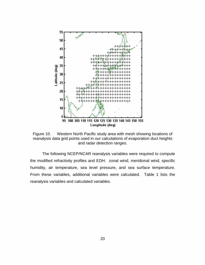
Figure 10. Western North Pacific study area with mesh showing locations of reanalysis data grid points used in our calculations of evaporation duct heights and radar detection ranges. ........................................... 20

Figure 11. Summary of the long range forecasting process developed and applied in our study. ........................................................................... 25

x

Figure 12. Two by two contingency table used in our study to categorize and assess our hindcast and forecast results............................................ 26

Figure 13. January LTM air temperature (oC) at 1000 hPa. Relatively cool (warm) air can be seen over the northern (southern portion) of the WNP AOI (boxed region) for this study. The cool air is asscoaited with the southward outflow of cold dry air along the eastern flank of the Siberian high (see Figures 14-15). Basic figure created at ESRL web site (http://www.cdc.noaa.gov, accessed May 2009). ....... 30

Figure 14. January LTM 1000 hPa geopotential height (m). The WNP AOI (boxed region) for our study occurs on the eastern flank of the Asian High (H) and near the western flank of the Aleutian Low (L) and North Pacific High (centered between Hawaii and California). Climate scale variations in these three height centers can lead to variations in the WNP AOI. Basic figure created at ESRL web site (http://www.cdc.noaa.gov, accessed May 2009). ............................... 31

Figure 15. January LTM 850 hPa vector wind (m/s). The northern (southern) portion of the WNP AOI (boxed region) for our study experiences predominantly southward (westward) low level winds. Northerly winds can be seen over the Korean penninsula as a result of the tightened gradient between the Siberian high and the Aluetian low while warm moist air is coming from the easterlies. Basic figure created at ESRL web site (http://www.cdc.noaa.gov, accessed May 2009). ................................................................................................. 32

Figure 16. January LTM sea surface temperature (SST; oC). The northern (southern) portion of the WNP AOI (boxed region) for our study experiences relatively warm (cool) SSTs, with strong SST gradients near the Korean peninsula. Basic figure created at ESRL web site (http://www.cdc.noaa.gov, accessed May 2009). ............................... 33

Figure 17. April LTM air temperature (°C) at 1000 hPa. When compared to January, April air temperature is greater over the entire WNP AOI (boxed region), with the largest change being over the Sea of Japan and the northern portion of the East China Sea. Basic figure created at ESRL web site (http://www.cdc.noaa.gov, accessed May 2009). ................................................................................................. 34

Figure 18. April LTM 1000 hPa geopotential height (m). Winter to spring changes in the WNP AOI (boxed region) are strongly influenced by the weakening of the Asian High and the strengthening of the North Pacific High from January to April. Basic figure created at ESRL web site (http://www.cdc.noaa.gov, accessed May 2009. .................. 34

Figure 19. April LTM 850 hPa vector wind (m/s). Note the shift from predoimnantly northerly winds over much of the WNP AOI (boxed region) in January to westerly and southerly winds in April. Basic figure created at ESRL web site (http://www.cdc.noaa.gov, accessed May 2009). ......................................................................... 35

xi

Figure 20. April LTM sea surface temperature (SST; °C). Note the increase in SSTs throughout the entire WNP AOI (boxed region) from January to April. Basic figure created at ESRL web site (http://www.cdc.noaa.gov, accessed May 2009). ............................... 35

Figure 21. July LTM air temperature (°C) at 1000 hPa. The WNP AOI (boxed region) is dominated by warm, moist air and weaker temperature gradients than in January and April. Basic figure created at ESRL web site (http://www.cdc.noaa.gov, accessed May 2009). ................. 36

Figure 22. July LTM 1000 hPa geopotential height (m). The dominant geopotential height patterns for the WNP AOI (boxed region) are the Asian Low and North Pacific High which cause mainly southerly flow over most of the AOI. Basic figure created at ESRL web site (http://www.cdc.noaa.gov, accessed May 2009). ............................... 37

Figure 23. July LTM 850 hPa vector wind (m/s). Winds are predominantly southerly over most of the WNP AOI (boxed region) consistent with advection of warm, moist air into the AOI from the tropics. LTM wind speeds in the AOI during summer tend to be weaker than in the other seasons. Basic figure created at ESRL web site (http://www.cdc.noaa.gov, accessed May 2009). ............................... 37

Figure 24. July LTM sea surface temperature (SST; °C). SSTs in the WNP AOI (boxed region) during summer are warmer and warmer than in the other seasons. Basic figure created at ESRL web site (http://www.cdc.noaa.gov, accessed May 2009). ............................... 38

Figure 25. October LTM air temperature (°C) at 1000 hPa. Cool low level air temperatures and SSTs develop during fall over East Asia and most of the WNP AOI (boxed region). Basic figure created at ESRL web site (http://www.cdc.noaa.gov, accessed May 2009). ................. 39

Figure 26. October LTM 1000 hPa geopotential height (m). During fall, the WNP AOI (boxed region) is strongly affected by the development of the Asian High, the southward shift and strengthening of the Aleutian Low, and the weakening and eastward shift of the North Pacific High. Basic figure created at ESRL web site (http://www.cdc.noaa.gov, accessed May 2009). ............................... 39

Figure 27. October LTM 850 hPa vector wind (m/s). In fall, the northern (southern) portion of the WNP AOI (boxed region) is doimnated by northerly (easterly) low level winds. Basic figure created at ESRL web site (http://www.cdc.noaa.gov, accessed May 2009). ................. 40

Figure 28. October LTM sea surface temperature (SST; °C). In fall, SSTs over most of the WNP AOI (boxed region) transition from warm summer conditions to cool winter conditions. Basic figure created at ESRL web site (http://www.cdc.noaa.gov, accessed May 2009). ................. 40

Figure 29. January LTM EDH (m) for the WNP AOI. ........................................... 42 Figure 30. January LTM wind speed (m/s) at 10 meters for WNP AOI................ 42 Figure 31. January LTM air-sea temperature difference (°C) for WNP AOI......... 43 Figure 32. January LTM relative humidity (%) at 2 meters for WNP AOI............. 43

xii

Figure 33. April LTM EDH (m) for the WNP AOI.................................................. 44 Figure 34. April LTM wind speed (m/s) at 10 meters for WNP AOI. .................... 45 Figure 35. April LTM air-sea temperature difference (°C) for WNP AOI. ............. 45 Figure 36. April LTM relative humidity (%) at 2 meters for WNP AOI. ................. 46 Figure 37. July LTM EDH (m) for the WNP AOI. ................................................. 47 Figure 38. July LTM wind speed (m/s) at 10 meters for WNP AOI. ..................... 47 Figure 39. July LTM air-sea temperature difference (°C) for WNP AOI. .............. 48 Figure 40. July LTM relative humidity (%) at 2 meters for WNP AOI. .................. 48 Figure 41. October LTM EDH (m) for the WNP AOI. ........................................... 49 Figure 42. October LTM wind speed (m/s) at 10 meters for WNP AOI................ 50 Figure 43. October LTM air-sea temperature difference (°C) for WNP AOI......... 50 Figure 44. October LTM relative humidity (%) at 2 meters for WNP AOI............. 51 Figure 45. January LTM RDR (nmi) for WNP AOI. .............................................. 52 Figure 46. April LTM RDR (nmi) for WNP AOI..................................................... 53 Figure 47. July LTM RDR (nmi) for WNP AOI. .................................................... 53 Figure 48. October LTM RDR (nmi) for WNP AOI. .............................................. 54 Figure 49. October conditional composite of surface winds for the five years

with the highest meridional wind speeds avearged over 20-28°N, 123-128°E (area east of Taiwan shown in Figure 9). From Turek (2008). ................................................................................................ 56

Figure 50. October conditional composite of surface winds for the five years with the lowest meridional wind speeds avearged over 20-28°N, 123-128°E (area east of Taiwan shown in Figure 9). From Turek (2008). ................................................................................................ 56

Figure 51. October conditional composite anomaly of surface winds for the five years with the highest meridional wind speeds avearged over 20-28°N, 123-128°E (area east of Taiwan shown in Figure 9). From Turek (2008). ...................................................................................... 57

Figure 52. October conditional composite anomaly of surface winds for the five years with the lowest meridional wind speeds avearged over 20-28°N, 123-128°E (area east of Taiwan shown in Figure 9). From Turek (2008). ...................................................................................... 57

Figure 53. Correlation of October radar detection range (RDR) in the focus region east of Taiwan (purple box) with SST in October for the years 1970-2006. The RDR is for a 9 GHz radar at 85 ft above the surface, looking for a 4 ft target with a detection threshold of 150 dB. The red box highlights a region of persistently high correlations when SST leads October RDR by zero to five months (see Figures 55-59). Basic figure created at ESRL web site (http://www.cdc.noaa.gov, accessed May 2009). ............................... 60

Figure 54. Correlation of October radar detection range (RDR) in the focus region east of Taiwan (purple box) with SST in September for the years 1970-2006. The RDR is for a 9 GHz radar at 85 ft above the surface, looking for a 4 ft target with a detection threshold of 150 dB. The red box highlights a region of persistently high correlations

xiii

when SST leads October RDR by zero to five months (see Figures 55-59). Basic figure created at ESRL web site (http://www.cdc.noaa.gov, accessed May 2009). ............................... 61

Figure 55. Correlation of October radar detection range (RDR) in the focus region east of Taiwan (purple box) with SST in August for the years 1970-2006. The RDR is for a 9 GHz radar at 85 ft above the surface, looking for a 4 ft target with a detection threshold of 150 dB. The red box highlights a region of persistently high correlations when SST leads October RDR by zero to five months (see Figures 55-59). Basic figure created at ESRL web site (http://www.cdc.noaa.gov, accessed May 2009). ............................... 62

Figure 56. Correlation of October radar detection range (RDR) in the focus region east of Taiwan (purple box) with SST in July for the years 1970-2006. The RDR is for a 9 GHz radar at 85 ft above the surface, looking for a 4 ft target with a detection threshold of 150 dB. The red box highlights a region of persistently high correlations when SST leads October RDR by zero to five months (see Figures 55-59). Basic figure created at ESRL web site (http://www.cdc.noaa.gov, accessed May 2009). ............................... 63

Figure 57. Correlation of October radar detection range (RDR) in the focus region east of Taiwan (purple box) with SST in June for the years 1970-2006. The RDR is for a 9 GHz radar at 85 ft above the surface, looking for a 4 ft target with a detection threshold of 150 dB. The red box highlights a region of persistently high correlations when SST leads October RDR by zero to five months (see Figures 55-59). Basic figure created at ESRL web site (http://www.cdc.noaa.gov, accessed May 2009). ............................... 64

Figure 58. Verification metrics for hindcasts for 1970-2006 of above normal (i.e., high) meridonal wind in October in the WNP focus region using eqatorial SST near the dateline in October, September, August, July, and June as the predictor. The hindcast methods, and the metrics and metrics legend acronyms are explained in Chapter II, section B. See text for additonal details. .......................... 65

Figure 59. Verification metrics for hindcasts for 1970-2006 of above normal (i.e., high) EDH in October in the WNP focus region using eqatorial SST near the dateline in October, September, August, July, and June as the predictor. The hindcast methods, and the metrics and metrics legend acronyms are explained in Chapter II, section B. See text for additonal details. ............................................................. 66

Figure 60. Verification metrics for hindcasts for 1970-2006 of near normal RDR in October in the WNP focus region using eqatorial SST near the dateline in October, September, August, July, and June as the predictor. The hindcast methods, and the metrics and metrics legend acronyms are explained in Chapter II, section B. See text for additonal details. ........................................................................... 66

xiv

Figure 61. October LTM evaporation duct height (EDH) example of the present U. S. Navy LTM EDH climatology in tabular format. .............. 68

Figure 62. October LTM evaporation duct height (EDH) example of the present U. S. Navy LTM EDH climatology, after we manually entered and then plotted the data shown in Figure 61........................ 69

Figure 63. October LTM evaporation duct height (EDH) example of applying modern climate data sets and methods to develop a state-of-the-science EDH climatology. Note the large differences between this modern EDH climatology and the present Navy climatology (Figure 61-62). ................................................................................................ 69

Figure 64. February LTM EDH (m) for the WNP AOI. ......................................... 75 Figure 65. March LTM EDH (m) for the WNP AOI............................................... 75 Figure 66. May LTM EDH (m) for the WNP AOI. ................................................. 76 Figure 67. June LTM EDH (m) for the WNP AOI. ................................................ 76 Figure 68. August LTM EDH (m) for the WNP AOI.............................................. 77 Figure 69. September LTM EDH (m) for the WNP AOI. ...................................... 77 Figure 70. November LTM EDH (m) for the WNP AOI. ....................................... 78 Figure 71. December LTM EDH (m) for the WNP AOI. ....................................... 78 Figure 72. February LTM RDR (nmi) for WNP AOI. ............................................ 79 Figure 73. March LTM RDR (nmi) for WNP AOI.................................................. 79 Figure 74. May LTM RDR (nmi) for WNP AOI. .................................................... 80 Figure 75. June LTM RDR (nmi) for WNP AOI. ................................................... 80 Figure 76. August LTM RDR (nmi) for WNP AOI................................................. 81 Figure 77. September LTM RDR (nmi) for WNP AOI. ......................................... 81 Figure 78. November LTM RDR (nmi) for WNP AOI. .......................................... 82 Figure 79. December LTM RDR (nmi) for WNP AOI. .......................................... 82 Figure 80. October conditional composite based on the five shortest RDR

years of a generic radar...................................................................... 83 Figure 81. October conditional composite based on the five longest RDR

years of a generic radar...................................................................... 83 Figure 82. October conditional anomaly based on the five shortest RDR years

of a generic radar. .............................................................................. 84 Figure 83. October conditional anomaly based on the five longest RDR years

of a generic radar. .............................................................................. 84 Figure 84. October LTM of RDR (nmi) for a generic radar. ................................. 85 Figure 85. October conditional composite based on the five lowest EDH years.. 85 Figure 86. October conditional composite based on the five highest EDH years 86 Figure 87. October conditional anomaly based on the five lowest EDH years. ... 86 Figure 88. October conditional anomaly based on the five highest EDH years. .. 87

xv

LIST OF TABLES

Table 1. Reanalysis variables and variables calculated from reanalysis variables that were used in this study. Not App means not applicable. .......................................................................................... 21

xvi


xvii

LIST OF ACRONYMS AND ABBREVIATIONS

14WS 14th Weather Squadron

AFW Air Force Weather

AOI Area of Interest

APM Advanced Propagation Model

AREPS Advanced Refractive Effects Prediction System

ASOS Automated Surface Observing Station

ASTD Air-Sea Temperature Difference

ASW Anti-Submarine Warfare

ATMS Atmosphere

BonD Battlespace on Demand

CDC Climate Diagnostics Center

CSI Critical Success Index

dB Decibel

DoD Department of Defense

ECS East China Sea

EDH Evaporation Duct Height

EN El Nino

ENSO El Nino Southern Oscillation

EOF Empirical Orthogonal Function

ESM Electronic Support Measures

ESRL Earth System Research Laboratory

FAR False Alarm Rate

HSS Heidke Skill Score

xviii

IDM Indian Dipole Mode

IOZM Indian Ocean Zonal Mode

LN La Nina

LRF Long Range Forecast

LTM Long-Term Mean

MEI Multivariate ENSO Index

METOC Meteorology and Oceanography

MJO Madden-Julian Oscillation

NCEP National Centers for Environmental Prediction

NCAR National Center for Atmospheric Research

nmi Nautical Mile

NOAA National Oceanic & Atmospheric Administration

NPS Naval Postgraduate School

PC Percent Correct

RDR Radar Detection Range

SCS South China Sea

SST Sea Surface Temperature

TS Threat Score

U.S. United States

WNP Western North Pacific

xix

ACKNOWLEDGMENTS

I would like to thank Fleet Numerical Meteorology and Oceanography

Center for offering me the opportunity to attend the Naval Postgraduate School.

I would like to recognize my advisors, Dr. Tom Murphree and Mr. Paul

Frederickson, for all their guidance and patience. Many thanks go to Mr. Bob

Creasey for retrieving reanalysis data that is the backbone of this thesis.

I owe a large debt of appreciation to my parents for always supporting and

believing in me. To my friends, I am grateful for the encouragement and support

throughout this educational journey.

xx


1

I. INTRODUCTION

A. MOTIVATION

The focus of this study is the long range prediction of radar detection

ranges (RDRs) for planning anti-submarine warfare (ASW) operations. With

knowledge of expected RDRs in the area of interest at long lead times, an

operational planner can make more effective decisions regarding offensive or

defensive ASW tactics. More skillful long range environmental forecasts will give

operational planners a better understanding of what types of environmental

scenarios to expect leading to more insightful decisions concerning, for example,

platform positioning in the area of operations.

Presently, the planning of ASW operations and naval operations in

general, begins on the order of three to six months before the operation starts.

For environmental information, the planners of these operations generally rely on

Navy climatologies that describe the estimated long term mean conditions that

have occurred in the past. These climatologies are generally based on outdated

data sets and analysis methods. Long range forecasts (LRFs; lead times of two

weeks or longer) are almost never available to the planners. In this study, we

investigated the use of modern data sets and methods for developing state-of-

the-science climate analyses and long range environmental predictions.

Much of the motivation for this study came from comparing existing U. S.

Navy climatologies with new experimental climate products developed using

modern methods. Figure 1 shows a comparison of traditional and modern, or

smart, climatology from Twigg (2007) for the evaporation duct height (EDH), a

key variable in determining RDRs. As explained in Twigg (2007), the traditional

EDH climatology provides information in text format only and is based on

outdated data sets and data analysis methods. The smart EDH climatology is

2

provided in graphical map format and is based on advanced data sets and data

analysis methods, and gives more accurate and reliable results at much higher

spatial and temporal resolutions.

Figure 1 Evaporation duct height (EDH, in m) for September from: (a) NPS smart EDH climatology and (b) existing Navy climatology. NPS smart

climatology devoloped from existing civilian multi-decadal atmospheric and oceanic reanalysis data sets. From Twigg (2007).

B. DEFINITIONS

1. Smart Climatology

Smart climatology, or warfighter climatology, is a concept developed by

Dr. Tom Murphree and Rear Admiral David Titley. It can be defined as state-of

the-science basic and applied climatology that directly supports Department of

Defense (DoD) operations. Smart climatology involves the use of state-of-the-

science data sets, data access and visualization tools, statistical and dynamical

analysis, climate modeling, climate prediction, and climate science decision

analysis and support tools for risk assessment, mitigation, and exploitation

(Murphree 2008a).

a b

3

2. Traditional Climatology

Traditional climatology is defined in this study as the climatological

methods currently employed by the U. S. Navy. Traditional climatology relies

mainly on long term mean (LTM) descriptions of climate system variables that

are of interest to warfighters. In some cases, LTMs provide useful guidance for

planners. But in many other cases, LTMs do not accurately depict the present or

future state of the climate system. This is largely because: (a) many of the LTMs

used in Navy climatology are based on inadequate and/or outdated data sets;

and (b) the climate system undergoes large variations that LTMs cannot explicitly

describe. For example, some Navy climatologies are constructed in part from

observational sea surface temperature data from ships during the period 1854-

1997. These climatologies differ significantly from those based on more recent

observations, analyses, and reanalyses. This is in part because the former data

set is: (a) sparse in many areas, especially outside of common shipping lanes

and for times of infrequent ship travel due to inclement weather; and (b) not up to

date and so does not represent the most recent decade(s). Modern or smart

climatologies emphasize the use of data sets and methods that compensate for

the shortcomings of traditional climatologies by, for example, focusing on data

from all reliable sources, data from the satellite era (e.g., 1970 onward), and

modern reanalysis methods for providing consistent multi-decadal, and state-of-

the-science descriptions of the climate system.

3. Smart Climatology Processes

The smart climatology process has been described and evaluated in many

studies, and through interactions between warfighters and Naval Postgraduate

School (NPS) faculty and students (e.g., LaJoie 2006; Hanson 2007;

Montgomery 2008; Moss 2007; Tournay 2008; Turek 2008; Twigg 2007;

Mundhenk 2009). Figure 2 shows the process that the NPS smart climatology

team uses to provide smart climatology support. The process starts with

identifying customer needs, timeline for completion, and the climate support

4

products that will be most beneficial for warfighters. In step two, information

about the mission (e.g., dates, objectives, operational thresholds) are used to

design the development and delivery of the climate support products. Step three

is to obtain and assess the required resources, for example, the appropriate data

sets, and analysis and prediction tools. In step four, the data sets and tools are

used to conduct analyses and produce predictions of the relevant environmental

conditions. The environmental predictions are then applied to tactical decision

aids and other tools to produce: (a) predictions of the operational impacts of the

expected environmental conditions; and (b) recommendations for how to deal

with the predicted impacts. The overall result of step five is a smart climatology

product support package delivered to military planners. The final step in the

smart climatology process is to verify, validate, and assess the operational value

of the support process and resulting support package.

Figure 2. The smart climatology process. From LaJoie (2006).

4. Smart Climatology Elements and Gaps in Military Support

Figure 3 shows the seven major elements of climate support identified by

Murphree (2008a). This figure also compares the overall status of operational

5

climate support by operational civilian climate centers and military climate

centers. For all seven elements, military support lags civilian support, with the

status of military support being comparable to the status of civilian support

several decades ago. In the last 5-10 years, the Navy meteorology and

oceanography (METOC) and Air Force Weather (AFW) communities have

become increasingly aware of these gaps in the climate support they provide.

However, the will and the resources to correct these gaps have been minimal, so

far. One motivation for this study is to provide additional evidence of the gaps in

military climate support, identify feasible methods for rapidly filling those gaps,

and make recommendations on how to quickly improve military climate support

capabilities. Many improvements are possible at relatively low cost by adapting

existing civilian data sets and methods that are available at little or no cost

(Murphree 2008a).

Figure 3. A comparison of the status of routine, readily available, operational climate support from operational civilian and military centers.in terms of the

seven major elements of climate support. From Murphree (2008a).

5. Smart Climatology and Battlespace on Demand (BonD)

Figure 4 illustrates the Battlespace on Demand (BonD) concept was

developed by the Navy METOC community to define the process by which the

U. S. Navy provides environmental support to warfighters. BonD has four tiers,

6

each representing a different step in providing support. The first step, known as

Tier 0, represents the development of environmental data sets. Tier 1 represents

the use of the data sets and various analysis and forecasting tools to describe

and predict the environment. Tier 2 represents the development of analyses and

predictions of how the environment affects military equipment (e.g., radar, sonar,

ships). Tier 3 describes the development of analyses and recommendations for

military planners on how best to exploit environmental opportunities and mitigate

environmental risks.

The BonD concept was developed to describe short range support (e.g.,

support provided at lead times of five days or less), but the concept also applies

to long lead support, including climate support. In Figure 4, the pink text boxes

identify smart climatology products associated with each of the four BonD tiers.

In this study, we developed examples of smart climatology products for all four

BonD tiers, including climate scale analyses and long range forecasts of radar

detection ranges, which are examples of a Tier 2 and 3 products.

Figure 4. Schematic depiction of the Battlespace on Demand (BonD) including descriptions of smart climatology support products for each of the four

BonD tiers. From Murphree (2008a).

7

C. RADAR TACTICAL DECISION AIDS

1. Definitions

a. Propagation Loss

Radar propagation loss is defined as the ratio of the transmitted

power over the received power (assuming the antenna patterns are normalized

to unity gain) at a given point in space. Propagation loss is expressed in terms of

decibels (dB).

b. Radar Detection Range

For the purposes of this study, radar detection range (RDR) is

defined as the maximum distance from a radar antenna at which a specific target

can be detected by a given radar system. RDR is sometimes referred to as the

target detection range. In order to estimate RDR, the propagation loss versus

range at the target height first needs to be computed. A target can theoretically

be detected where the propagation loss is less than the detection threshold

value, and cannot be detected where the propagation loss is greater than the

threshold. The RDR can therefore be defined as the maximum distance from a

radar at which the propagation loss equals the detection threshold. The

detection threshold value is a function of the radar system attributes and the

target’s size, shape, composition, and orientation with respect to incident radar

waves. The RDR as defined above is only an approximation, although often a

very good approximation, of the actual range at which a surface or low altitude

target might be detected in a real-world situation. Radar target detection

depends on other factors in addition to the propagation loss, such as sea clutter,

system signal-to-noise ratios, and the signal filtering and target recognition

procedures being employed.

8

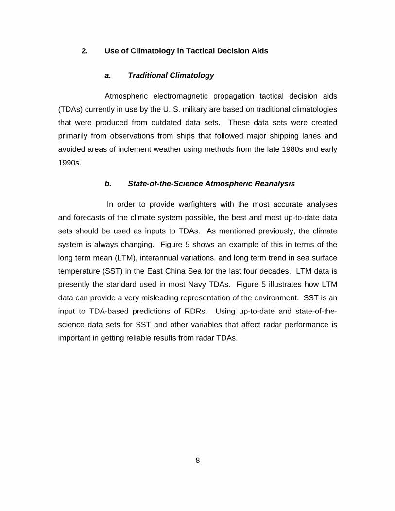
2. Use of Climatology in Tactical Decision Aids

a. Traditional Climatology

Atmospheric electromagnetic propagation tactical decision aids

(TDAs) currently in use by the U. S. military are based on traditional climatologies

that were produced from outdated data sets. These data sets were created

primarily from observations from ships that followed major shipping lanes and

avoided areas of inclement weather using methods from the late 1980s and early

1990s.

b. State-of-the-Science Atmospheric Reanalysis

In order to provide warfighters with the most accurate analyses

and forecasts of the climate system possible, the best and most up-to-date data

sets should be used as inputs to TDAs. As mentioned previously, the climate

system is always changing. Figure 5 shows an example of this in terms of the

long term mean (LTM), interannual variations, and long term trend in sea surface

temperature (SST) in the East China Sea for the last four decades. LTM data is

presently the standard used in most Navy TDAs. Figure 5 illustrates how LTM

data can provide a very misleading representation of the environment. SST is an

input to TDA-based predictions of RDRs. Using up-to-date and state-of-the-

science data sets for SST and other variables that affect radar performance is

important in getting reliable results from radar TDAs.

9

Figure 5. Sea surface temperature (SST; C°) in the East China Sea for July - September of 1968-2006. Traditional climatology describes the long term mean SST and related quantities (e.g., the long term mean high and low SST) shown

by the solid and dashed blue lines. But traditional climatology does not describe interannual variations (identified by red ovals), long term trends (identified by red

line), and other deviations from long trm mean conditions.

3. Naval Postgraduate School Bulk Model

The Naval Postgraduate School (NPS) has created a state-of-the-science

operational bulk evaporation duct model that computes the near-surface modified

refractivity profile and evaporation duct height from measured or modeled values

of wind speed, air and sea temperature, relative humidity, and atmospheric

pressure. The NPS model is based on Monin-Obukhov similarity theory and is

therefore only valid within the atmospheric surface layer, which extends upwards

on the order of 10 to 100 meters above the surface, depending on atmospheric

stratification conditions. The model uses a modified form of the TOGA-COARE

bulk algorithm to compute the surface layer scaling parameters, which are then

used to compute the modified refractivity profile up to a height of 100 m. The

evaporation duct height is determined by finding the height of the local minimum

in the modified refractivity profile that occurs nearest to the surface. In order to

prevent erroneous solutions from the model, the NPS model incorporates

operational checks on all input data and flags any impossible or unrealistic

10

cases. The modified refractivity profile is used as the environmental input to

electromagnetic propagation models, such as the Advanced Propagation Model

(APM) described in the next section.

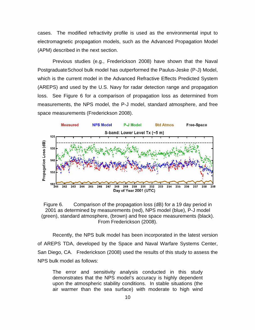
Previous studies (e.g., Frederickson 2008) have shown that the Naval

Postgraduate School bulk model has outperformed the Paulus-Jeske (P-J) Model,

which is the current model in the Advanced Refractive Effects Predicted System

(AREPS) and used by the U.S. Navy for radar detection range and propagation

loss. See Figure 6 for a comparison of propagation loss as determined from

measurements, the NPS model, the P-J model, standard atmosphere, and free

space measurements (Frederickson 2008).

Figure 6. Comparison of the propagation loss (dB) for a 19 day period in 2001 as determined by measurements (red), NPS model (blue), P-J model

(green), standard atmosphere, (brown) and free space measurements (black). From Frederickson (2008).

Recently, the NPS bulk model has been incorporated in the latest version

of AREPS TDA, developed by the Space and Naval Warfare Systems Center,

San Diego, CA. Frederickson (2008) used the results of this study to assess the

NPS bulk model as follows:

The error and sensitivity analysis conducted in this study demonstrates that the NPS model’s accuracy is highly dependent upon the atmospheric stability conditions. In stable situations (the air warmer than the sea surface) with moderate to high wind

11

speeds and humidity, the model may perform adequately well for propagation modeling purposes. With large positive air-sea temperature differences and low wind and humidity, however, the model results become highly suspect because Monin-Obukhov similarity theory, upon which the model is based, begins to break down in such low-turbulence situations. In addition, the model becomes extremely sensitive to the input parameters in highly stable conditions. In some cases evaporation duct height errors can exceed 4 m as a result of only modest uncertainties in the model inputs. In unstable conditions (the air colder than the sea surface), the NPS model produces highly accurate evaporation duct and refractivity profile information, suitable for high-fidelity propagation modeling applications. Fortunately, unstable conditions are the most prevalent situation over the world’s oceans. The error and sensitivity analysis in this study demonstrated that when provided with high quality input data the NPS model can determine the evaporation duct height with an accuracy of about 2 m or better in almost all unstable cases. When the NPS model is used in conjunction with modern propagation codes, such as the Advanced Propagation Model, near surface propagation loss predictions accurate to about 1-3 dB at a range of 30 km and 3-7 dB at 60 km can be expected in unstable conditions for a S-band radar. Near surface target detection range errors were estimated to be approximately 1-4 km for a target that is normally detectable at 30-35 km, and 2-8 km for a target normally detected at 50-70 km. Real-time propagation assessments and short-range forecasts with such accuracies would constitute a highly valuable tool for planning and executing naval and maritime operations. It must be noted that these accuracy estimates do not take into account potential errors due to temporal and spatial variations in atmospheric refractivity or surface scattering conditions, for example. (Frederickson 2008).

4. Advanced Propagation Model

We used the Advanced Propagation Model (APM) in our study to compute

the propagation loss for a specific height versus range coverage area. APM was

developed by the Atmospheric Propagation Branch of the Space and Naval

Warfare Systems Center, San Diego (Barrios and Patterson 2002) and uses a

hybrid ray-optic and parabolic equation model to compute the propagation loss.

In order to generate radar detection range analyses and forecasts, we used the

NPS bulk evaporation duct model to compute the modified refractivity profile,

12

which was then used as input to APM. APM then computed the propagation loss

versus range at the target height for a specific radar system, from which the

radar detection range was determined.

5. Advanced Refractive Effects Prediction System

The Advanced Refractive Effects Prediction System (AREPS) was

developed by the Space and Naval Warfare Systems Center, San Diego and is

used by the U. S. Navy to determine radar probability of detection, propagation

loss, and signal-to-noise ratios, electronic support measures (ESM) vulnerability,

UHF/VHF communications, and surface-borne surface-search radar capability

versus range, height, and bearing from a transmitter (Patterson 1987). For this

study, AREPS was used to determine the frequency of occurrence of evaporation

ducts over the western North Pacific (WNP), especially the East China Sea

(ECS), South China Sea (SCS), and surrounding waters. We used smart

climatology data sets and methods to develop the input fields for AREPS to

expand on what AREPS can provide and give warfighters climate analyses and

forecasts of radar performance for large regions, instead of the probability of

detection at specific point locations.

D. REFRACTION, DUCTING, AND RADAR DETECTION RANGES

Due to the common occurrence of evaporation ducts over the ocean and

their strong impact on near-surface radar propagation, it is important to

accurately predict the characteristics of evaporation ducts in order to estimate the

radar detection and tracking of submarine periscopes, low-flying missiles and

aircraft, and surface combatants. In our study, we focused on the ability to

predict radar detection ranges for submarine periscopes using surface ship-

based search radars. In the following sections we describe how the near-surface

atmospheric and sea surface conditions affect radar propagation and detection

ranges.

13

1. Modified Refractivity and Ducting Layers

Vertical and horizontal gradients of the refractive index of air determine

the propagation of electromagnetic radiation through the atmosphere. The

refractive index of air, n, is defined as the ratio of the speed of an

electromagnetic wave through a vacuum over the speed through air

(Frederickson 2008). Electromagnetic waves bend or refract toward regions of

higher n. The refractivity, denoted as N, describes the difference of n from unity

and is often used since n is always close to unity. For the radar wavelengths that

we used in our research, N is related to the atmospheric variables of absolute

temperature (T), partial pressure of water vapor (е), and total atmospheric

pressure (P) through the following equation (Bean and Dutton 1968):

52

77.6 5.6 3.75 10P e e

N xT T T

(1)

where T is in Kelvin, and P and е are in hPa.

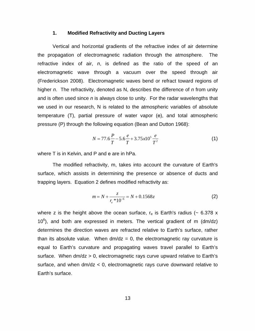
The modified refractivity, m, takes into account the curvature of Earth's

surface, which assists in determining the presence or absence of ducts and

trapping layers. Equation 2 defines modified refractivity as:

60.1568

*10e

zm N N z

r (2)

where z is the height above the ocean surface, re is Earth's radius (~ 6.378 x

106), and both are expressed in meters. The vertical gradient of m (dm/dz)

determines the direction waves are refracted relative to Earth’s surface, rather

than its absolute value. When dm/dz = 0, the electromagnetic ray curvature is

equal to Earth’s curvature and propagating waves travel parallel to Earth’s

surface. When dm/dz > 0, electromagnetic rays curve upward relative to Earth’s

surface, and when dm/dz < 0, electromagnetic rays curve downward relative to

Earth’s surface.

14

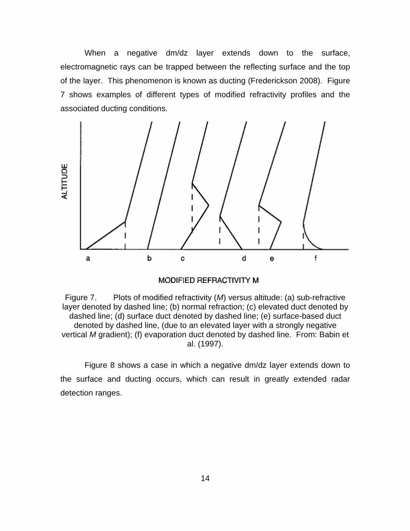
When a negative dm/dz layer extends down to the surface,

electromagnetic rays can be trapped between the reflecting surface and the top

of the layer. This phenomenon is known as ducting (Frederickson 2008). Figure

7 shows examples of different types of modified refractivity profiles and the

associated ducting conditions.

Figure 7. Plots of modified refractivity (M) versus altitude: (a) sub-refractive layer denoted by dashed line; (b) normal refraction; (c) elevated duct denoted by

dashed line; (d) surface duct denoted by dashed line; (e) surface-based duct denoted by dashed line, (due to an elevated layer with a strongly negative

vertical M gradient); (f) evaporation duct denoted by dashed line. From: Babin et al. (1997).

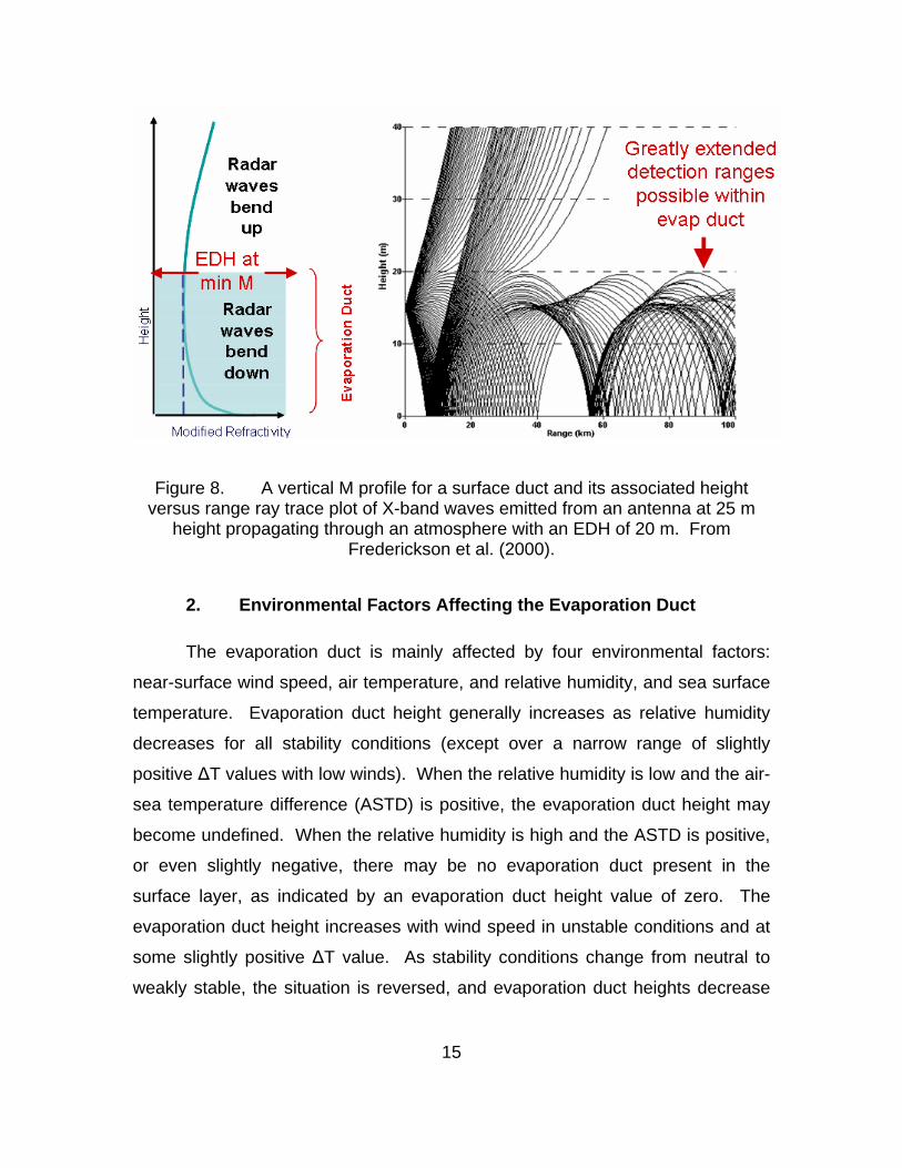
Figure 8 shows a case in which a negative dm/dz layer extends down to

the surface and ducting occurs, which can result in greatly extended radar

detection ranges.

15

Figure 8. A vertical M profile for a surface duct and its associated height versus range ray trace plot of X-band waves emitted from an antenna at 25 m

height propagating through an atmosphere with an EDH of 20 m. From Frederickson et al. (2000).

2. Environmental Factors Affecting the Evaporation Duct

The evaporation duct is mainly affected by four environmental factors:

near-surface wind speed, air temperature, and relative humidity, and sea surface

temperature. Evaporation duct height generally increases as relative humidity

decreases for all stability conditions (except over a narrow range of slightly

positive ΔT values with low winds). When the relative humidity is low and the air-

sea temperature difference (ASTD) is positive, the evaporation duct height may

become undefined. When the relative humidity is high and the ASTD is positive,

or even slightly negative, there may be no evaporation duct present in the

surface layer, as indicated by an evaporation duct height value of zero. The

evaporation duct height increases with wind speed in unstable conditions and at

some slightly positive ΔT value. As stability conditions change from neutral to

weakly stable, the situation is reversed, and evaporation duct heights decrease

16

with wind speed. For a given ASTD, the evaporation duct height generally

increases with increasing sea surface temperature (Frederickson 2008).

3. Electromagnetic Propagation and Detection Ranges

The best single parameter for quantifying near-surface microwave

propagation is the evaporation duct height (EDH). The EDH is a critical factor in

determining the near-surface refractivity conditions and higher EDHs often lead

to increased signal strength and radar detection ranges, depending upon the

frequency, and the height of the radar and target (Twigg 2007). Radar detection

ranges are estimated from the computed propagation loss by determining the

maximum distance where the propagation loss at the target height is equal to the

propagation loss detection threshold assumed for the target (Twigg 2007).

Propagation loss will decrease and the detection range will increase when the

radar and target are located within the duct. Even when the radar and target are

not located within the duct there can be some trapping of EM energy within it and

extended detection ranges are possible.

4. Current Radar Detection Range Products

Currently, the U. S. Navy provides few radar detection range products as

tactical guidance to warfighters. Forecast in the form of threshold-based stop-

light charts are produced at lead times of a couple days in advance. The

Advanced Refractive Effects Prediction System (AREPS) (see Chapter I, section

C, part 4) is used to plot electromagnetic propagation for specific sensor systems

and environmental conditions. These products rely on an outdated bulk

evaporation duct model and an outdated climatological data set. This study

examined the potential of state-of-the-science climate data sets and methods to

produce products for warfighters that are both more accurate representations of

the actual environment that will be encountered during an operation and more

relevant to warfighter needs.

17

E. OVERVIEW OF THIS STUDY

Our study addressed the following research questions:

1. Can state-of-the-science data sets and methods be used to create

a more accurate and useful characterization of atmospheric radar

propagation, and thus provide tactically significant improvements in

war fighting capabilities?

2. Can skillful long range forecasts of evaporation duct heights and

radar detection ranges be developed for mission planning

purposes?

We addressed these questions in the context of the western North Pacific

(WNP), centered on the East China Sea (ECS) and nearby waters (15-45oN, 95-

145oE; see Figure 9). We chose this as our study area because it is affected by

several major climate variations, it is operationally significant to the U. S. military,

and prior studies have shown skill at long range forecasting in this region (cf.

Ford 2000; Tournay 2008; Turek 2008; Mundhenk 2009). The WNP region

bounded by 20-28oN and 122-126oE (red box in Figure 9) was a focus area for

developing our long range forecasting methods.

18

Figure 9. Western North Pacific study region. The red box encompassing 20-28oN and 122-126oE was a focus area for developing our long range

forecasting methods.

Our data and methods are presented in Chapter II. In Chapter III, we

present our answers to our research questions. Chapter IV provides a summary

of our results, conclusions, and suggestions for future research.

19

II. DATA AND METHODS

A. DATA

The main environmental data used in this study was obtained from the

National Center for Environmental Prediction and the National Center for

Atmospheric Research (NCEP/NCAR) Reanalysis-1 data set. The data set was

obtained on March 20, 2009, via the National Oceanic & Atmospheric

Administration (NOAA) Climate Diagnostic Center (CDC) website

(http://www.cdc.noaa.gov). The NCEP/NCAR reanalysis-1 data set includes data

for a wide range of standard atmospheric variables plus sea surface temperature

(SST). The reanalysis data set has a 1.875° latitude by 1.875° longitude spatial

resolution, which is equivalent to about 210 km horizontal resolution, and a

temporal resolution of every 6 hours (0, 6, 12 and 18Z) (Kistler 2001). Figure 10

shows the reanalysis grid for our WNP study area, or area of interest (AOI). The

data set spans 61 years (1948 to present). However, for this study we only used

data from 1970-2008, based on our determination that the reanalysis data prior

to 1970 are less reliable, mainly due to a lack of significant amounts of satellite

data prior to the 1970s. This lack of data is especially significant for studies such

as ours that deal with environmental conditions over the ocean. The reanalysis

data set incorporates ship, land surface, satellite, rawinsonde, aircraft, and other

data sets. This data is assimilated via a T62 global spectral model with 28

vertical sigma levels (Kistler 2001). The vertical resolution of the reanalysis data

set is not high enough to explicitly resolve EM ducts just above the ocean

surface. However, the evaporation duct over the ocean can be characterized in

terms of surface quantities (see Chapter II, section D), so we were able to use

the reanalysis data to calculate EDHs and the related RDRs. The reader is

referred to Kalnay et al. (1996) and Kistler et al. (2001) for further details

regarding the reanalysis data set.

20

Figure 10. Western North Pacific study area with mesh showing locations of reanalysis data grid points used in our calculations of evaporation duct heights

and radar detection ranges.

The following NCEP/NCAR reanalysis variables were required to compute

the modified refractivity profiles and EDH: zonal wind, meridional wind, specific

humidity, air temperature, sea level pressure, and sea surface temperature.

From these variables, additional variables were calculated. Table 1 lists the

reanalysis variables and calculated variables.

21

Table 1. Reanalysis variables and variables calculated from reanalysis variables that were used in this study. Not App means not applicable.

B. METHODS

1. Evaporation Duct Height and Radar Detection Range Calculations

The six hourly wind speed, air and sea surface temperatures, relative

humidity, and atmospheric pressure data from the reanalysis data set were put

into the NPS bulk evaporation duct model for each grid point in our area of

interest. From these input data, the NPS model computed the modified

refractivity profile up to a height of 100 meters. The evaporation duct height

(EDH) was determined by finding the height closest to the surface at which the

local minima in modified refractivity occurred.

Next, the modified refractivity profile from the NPS model was put into

APM, which computed the propagation loss versus range for our radar

parameters at the height of our assumed target. The radar detection range

(RDR) was then estimated by finding the maximum distance from the radar

where the propagation loss at the target height was equal to the target detection

threshold value. Note that in this method we assumed that the environmental

22

conditions were horizontally homogeneous in the region near each grid point,

with no attempt being made to resolve spatial variations in refractivity conditions

near each grid point. The spatial variations were determined by the refractivity

differences between the grid points.

The evaporation duct height and radar detection range calculations

described above are only valid over the ocean. Reanalysis data for grid points

close to the coast represent information about conditions over both the land and

ocean. This means that an ocean grid point close to land may represent an

average of data from both over the land and the ocean. As an example, for such

a grid point the surface temperature would be an average of the sea surface

temperatures from the ocean areas of the grid box and the land skin

temperatures from the land areas. The resulting EDH values from a near shore

grid point can exhibit a very drastic change from adjacent grid boxes that are

entirely over the ocean. For this reason, EDH and RDR results near coastlines

should be treated with caution. To eliminate erroneous EDH and RDR

computations from near shore grid points, we created a land mask that

eliminated as many land values as possible that could affect our calculations.

2. Climate Analyses

We applied a number of standard climate analysis methods to develop our

climate scale analyses and long range forecasts of EDH and RDR in the WNP.

During our research, we used various techniques to manipulate the NCEP/NCAR

reanalysis data set in order to find deviations from the long term mean and

provide the most accurate radar detection ranges for our given environment.

To identify the major temporal variations, we broke the data for 1970-2006

into above normal (AN), near normal (NN), and below normal (BN) tercile

categories representing the upper, middle, and lower 33% of the values for each

variable of interest. This tercile information was used to: (a) identify years for

conditional compositing (see Chapter II, section 4) and long range forecast

23

development (see Chapter II, section 5); and (b) interpret the physical processes

that create climate variations and long range predictability in EDH and RDR in

the WNP.

Our analyses were facilitated by use of online tools for processing the

reanalysis data made available by the Earth Systems Research Laboratory

(ESRL; http://www.esrl.noaa.gov/). These tools, plus additional Excel and Matlab

based tools, were used to compute long term means, conditional composite

means, conditional composite anomalies, time series, and linear correlations.

The results of these calculations were used to identify and assess the climate

variations that determine how EDH and RDR, and the environmental factors that

determine them. Plots of radar detection ranges and evaporation duct heights

were generated using MATLAB (Mathworks 2005).

Linear correlation was used to identify relationships between different

climate system variables, EDH, and RDR. Correlations between variables at

widely separated locations provided us with information about the

teleconnections between the variables. Teleconnections describe how variations

in the environment at one location are related to those at distant location. In our

study, we used such correlations to determine how the environment factors,

EDH, and RDR in our WNP AOI were correlated with SST and other

environmental variables in remote locations. A two-tailed test was used to

determine the significance at a 95% confidence interval. The significance testing

for spatial correlations was based on the test statistic equation:

0.025zZ

n (3)

where: Z is the test statistic; 0.025z = standard normal distribution = 1.96 and n =

37 years (1970-2006). Z, or correlation, values greater than 0.318 are significant

at the 95% level. See Wilks (2006) for additional information on significance

testing.

24

We used conditional compositing to average together past events in which

conditions of interest were met. For example, we constructed conditional

composites of the conditions over the East China Sea (ECS) in October when

extreme conditions occurred — for example, when meridional winds were

exceptionally strong and weak (e.g., composites of the five highest and lowest

wind events) and when RDRs were exceptionally long and short (e.g.,

composites of the five longest and shortest RDR events). Using this technique

allows us to isolate and analyze the years of greatest variation in the climate

system.

We also analyzed how the conditional composites differed from the LTMs

by calculating conditional composite anomalies. For these calculations, the

conditional composite anomaly was defined as the conditional composite minus

the LTM, with the LTM calculated for the base period 1970-2006. The

conditional composite anomalies highlight the deviations from normal associated

with the conditional composites (e.g., how RDRs during high wind periods tend to

vary from LTM RDRs).

3. Forecasting

Figure 11 summarizes the processes used to produce long range

forecasts (LRFs) of the environmental factors, EDH, and RDR for the WNP AOI.

Step 1 involved identifying the predictands for which LRFs are produced. For our

study, the predictands of interest were meridional wind speed, EDH, and RDR in

the WNP AOI. Meridional wind was selected because of: (a) the prior work by

Turek (2008) that showed strong interannual variations of the meridional wind in

our WNP AOI; and (b) the importance of the meridional wind in the WNP AOI in

determining EDH via direct influences on ducting and via effects on the other

factors that determine EDH (air temperature, SST, and relative humidity). In step

2, correlations between the predictands and other environmental variables (e.g.,

SST in the tropical Pacific) were computed. These correlations were used in

step 3 to select the predictors with the most potential for producing skillful LRFs.

25

In step 4, hindcasts of the predictands were produced. The hindcast method was

based on using the correlation results, and AN, NN, and BN tercile break downs

of the predictands and predictors (see Chapter II, section B.2) to identify

predictable relationships between the predictors and predictands (e.g., AN SST

in the western central equatorial Pacific is strongly associated with BN meridional

winds in the WNP AOI). Hindcasts of monthly mean values of the predictands at

lead times of 0-5 months were done for the years 1970-2006. In step 5, the

hindcasts were verified against reanalysis monthly mean values using a variety

metrics calculated using contingency tables. The resulting metrics of hindcast

skill were used to identify the predictor-predictand relationships and the lead

times with a high potential for skillful LRFs. These high potential relationships and

lead times were then used to select develop the LRF method for each predictand. In

step 6, LRFs were produced using the methods identified in step 5.

Figure 11. Summary of the long range forecasting process developed and applied in our study.

26

4. Verification Metrics

a. Contingency Tables

In order to assess the hindcasts and forecasts, we needed to

determine what types of errors were made and to quantify the differences

between the predicted events and what actually occurred. Two by two

contingency tables (e.g., Figure 12) are commonly used to four possible

outcomes from forecasts: hits, misses, false alarms, and correct negatives (e.g.,

Wilks 2006). A perfect prediction would produce only hits and correct negatives.

Hits and correct negatives occur when the observed value equals that of the

forecast. A hit represents a case in which an event was forecasted and

observed. A correct negative represents a case in which an event was

forecasted not to occur and it did not occur. The following sub-sections describe

the main skill metrics we used to assess our hindcasts and forecasts. See Wilks

(2006) and the Australian Bureau of Meteorology web site for more information

on forecast verification metrics:

(http://www.bom.gov.au/bmrc/wefor/staff/eee/verif/verif_web_page.html)

Figure 12. Two by two contingency table used in our study to categorize and assess our hindcast and forecast results.

b. Percent Correct

The most direct and intuitive measure of non-probabilistic forecast

accuracy for discrete events is the percent correct (PC) proposed by Finley

(1884). This is simply the percent of forecasts that correctly anticipated the

subsequent event or non-event. The percent correct penalizes both kinds of

27

errors (false alarm and misses) equally. The best (worst) result is 100 (0). PC

was calculated as:

(3)

c. Probability of Detection

The probability of detection (POD) is defined as the percentage of

forecasts that correctly predicted the observed events. The best (worst) result is

100 (0). The POD was calculated as:

x 100 (4)

d. False Alarm Rate

The false alarm rate (F) is the percentage of forecasts that

forecasted events or non-events that did not happen. It is calculated as ratio of

false alarms to the total number of non-occurrences of the forecast event or the

conditional relative frequency of a wrong forecast given the event does not occur.

The best (worst) result is 0 (100). F was calculated as:

x 100 (5)

e. Threat Score

The threat score (TS; also known as the critical success index

(CSI)) is the number of correct yes forecasts divided by the total number of

occasions on which that event was forecast and/or observed. It can be viewed

as the proportion correct for the quantity being forecast, after removing correct no

forecasts from consideration. The best (worst) possible threat score is one

(zero). TS was computed as:

28

(6)

f. Heidke Skill Score

The Heidke Skill Score (HSS) describes the skill after subtracting

credit for accurate forecasts that could have been achieved by random

forecasting. Random forecasts define the standard or reference forecast against

which the actual forecasts are measured. HSS gives more (less) credit for

accurate forecasts of rare (common) events. The best HSS is one, a HSS of

zero indicates the forecasts have no skill with respect to the reference forecast,

and a HSS less than zero less skill than the reference forecast. We computed

HSS as:

(7)

C. SUMMARY

The data and methods used in this study are designed to design, develop,

and test methods for producing skillful long range forecasts of EDH and RDR

that can be used to improve long lead mission planning.

29

III. RESULTS

A. LONG TERM MEAN SEASONAL CYCLES: LARGE SCALE FEATURES AND PROCESSES

To develop methods for producing skillful LRFs of EDH and RDR in the

WNP, it is important to start with an understanding of the seasonal cycle of the

large scale features and processes that determine environmental conditions in

the WNP. To do so, we examined global scale patterns in surface air

temperature, 1000 hPa geopotential height, 850 hPa winds, and SST for winter

(January-March), spring (April-June), summer (July-September), and fall

(October-December), with a focus on the WNP in January, April, July, and

October.

1. Winter

Figures 13-16 show the January LTM surface air temperature, 1000 hPa

geopotential height, 850 hPa winds, and SST for most of the globe and centered

on the western North pacific area of interest (WNP AOI) for this study (14oN-

47oN, 105oE-148oE; see Figures 9-10). As described in the captions for these

figures, the AOI is strongly influenced by large scale atmospheric and oceanic

features over Asia, the North Pacific, and the tropical Pacific. The Asian High

and accompanying northerly winds along its eastern flank, are especially

important features in determining winter air temperature, relative humidities, and

winds over much of the AOI. The trade winds on the southern flank of the North

pacific High are important in determining conditions in much of the southern

portion of the AOI. The presence of strong gradients in air temperature,

geopotential heights, winds, and SST in and near the AOI, and the relationship of

these variables and their gradients to hemispheric scale climate features,

30

suggest that large climate variations are probably in the AOI during winter, and

are likely to be related via teleconnections to climate variations in distant

locations.

Figure 13. January LTM air temperature (oC) at 1000 hPa. Relatively cool (warm) air can be seen over the northern (southern portion) of the WNP AOI (boxed region) for this study. The cool air is asscoaited with the southward

outflow of cold dry air along the eastern flank of the Siberian high (see Figures 14-15). Basic figure created at ESRL web site (http://www.cdc.noaa.gov,

accessed May 2009).

31

Figure 14. January LTM 1000 hPa geopotential height (m). The WNP AOI (boxed region) for our study occurs on the eastern flank of the Asian High (H)

and near the western flank of the Aleutian Low (L) and North Pacific High (centered between Hawaii and California). Climate scale variations in these

three height centers can lead to variations in the WNP AOI. Basic figure created at ESRL web site (http://www.cdc.noaa.gov, accessed May 2009).

32

Figure 15. January LTM 850 hPa vector wind (m/s). The northern (southern) portion of the WNP AOI (boxed region) for our study experiences predominantly

southward (westward) low level winds. Northerly winds can be seen over the Korean penninsula as a result of the tightened gradient between the Siberian high and the Aluetian low while warm moist air is coming from the easterlies.

Basic figure created at ESRL web site (http://www.cdc.noaa.gov, accessed May 2009).

33

Figure 16. January LTM sea surface temperature (SST; oC). The northern (southern) portion of the WNP AOI (boxed region) for our study experiences

relatively warm (cool) SSTs, with strong SST gradients near the Korean peninsula. Basic figure created at ESRL web site (http://www.cdc.noaa.gov,

accessed May 2009).

2. Spring

Figures 17-20 show the April LTM surface air temperature, 1000 hPa


on the WNP AOI for this study. As noted in the captions for these figures, the

AOI experiences large seasonal changes in the transition from winter to spring.

These changes are closely linked to seasonal shifts in the intensity and location

of the Asian High, Aleutian Low, and North Pacific High. This transition causes

the AOI to become more tropical in character — for example, via the replacement

over much of the AOI of cold, dry air with warm, moist air, and of strong northerly

winds with weaker westerly and southerly winds.

34

Figure 17. April LTM air temperature (°C) at 1000 hPa. When compared to January, April air temperature is greater over the entire WNP AOI (boxed region), with the largest change being over the Sea of Japan and the northern portion of

the East China Sea. Basic figure created at ESRL web site (http://www.cdc.noaa.gov, accessed May 2009).

Figure 18. April LTM 1000 hPa geopotential height (m). Winter to spring changes in the WNP AOI (boxed region) are strongly influenced by the

weakening of the Asian High and the strengthening of the North Pacific High from January to April. Basic figure created at ESRL web site

(http://www.cdc.noaa.gov, accessed May 2009.

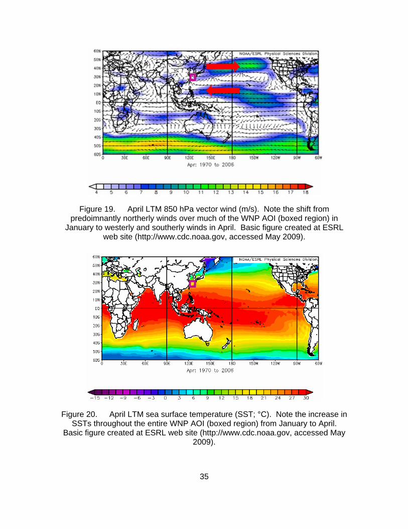
35

Figure 19. April LTM 850 hPa vector wind (m/s). Note the shift from predoimnantly northerly winds over much of the WNP AOI (boxed region) in

January to westerly and southerly winds in April. Basic figure created at ESRL web site (http://www.cdc.noaa.gov, accessed May 2009).

Figure 20. April LTM sea surface temperature (SST; °C). Note the increase in SSTs throughout the entire WNP AOI (boxed region) from January to April.

Basic figure created at ESRL web site (http://www.cdc.noaa.gov, accessed May 2009).

36

3. Summer

Figures 21-24 show the July LTM surface air temperature, 1000 hPa


on the WNP AOI for this study. The AOI in summer experiences warm moist

conditions with: (a) relatively weak temperature gradients; and (b) winds that are

generally southerly and weak compared to winter. These conditions are closely

linked to seasonal shifts in the intensity and location of the Asian Low, Aleutian

Low, and North Pacific High. In particular, the northward retreat of the Aleutian

Low, the development of the Asian Low, and the strengthening of the North

Pacific High lead to southerly low level winds over the AOI and the advection of

warm moist tropical marine air into the AOI.

Figure 21. July LTM air temperature (°C) at 1000 hPa. The WNP AOI (boxed region) is dominated by warm, moist air and weaker temperature gradients than

in January and April. Basic figure created at ESRL web site (http://www.cdc.noaa.gov, accessed May 2009).

37

Figure 22. July LTM 1000 hPa geopotential height (m). The dominant geopotential height patterns for the WNP AOI (boxed region) are the Asian Low and North Pacific High which cause mainly southerly flow over most of the AOI. Basic figure created at ESRL web site (http://www.cdc.noaa.gov, accessed May

2009).

Figure 23. July LTM 850 hPa vector wind (m/s). Winds are predominantly southerly over most of the WNP AOI (boxed region) consistent with advection of

warm, moist air into the AOI from the tropics. LTM wind speeds in the AOI during summer tend to be weaker than in the other seasons. Basic figure created at ESRL web site (http://www.cdc.noaa.gov, accessed May 2009).

38

Figure 24. July LTM sea surface temperature (SST; °C). SSTs in the WNP AOI (boxed region) during summer are warmer and warmer than in the other seasons. Basic figure created at ESRL web site (http://www.cdc.noaa.gov,

accessed May 2009).

4. Fall

Figures 25-28 show the October LTM surface air temperature, 1000 hPa


on the WNP AOI for this study. The AOI in fall transitions from warm, moist

conditions with relatively weak southerly winds toward the winter conditions show

cold, dry, and strong northerly wind conditions of winter (Figures 13-18). There

placement of the Asian Low by the developing Asian High, the southward shift

and strengthening of the Aleutian Low, and the strengthening and eastward shift

of the North Pacific High lead to the onset of northerly low level winds over the

AOI and the advection of cool, dry continental air into the AOI.

39

Figure 25. October LTM air temperature (°C) at 1000 hPa. Cool low level air temperatures and SSTs develop during fall over East Asia and most of the WNP

AOI (boxed region). Basic figure created at ESRL web site (http://www.cdc.noaa.gov, accessed May 2009).

Figure 26. October LTM 1000 hPa geopotential height (m). During fall, the WNP AOI (boxed region) is strongly affected by the development of the Asian

High, the southward shift and strengthening of the Aleutian Low, and the weakening and eastward shift of the North Pacific High. Basic figure created at

ESRL web site (http://www.cdc.noaa.gov, accessed May 2009).

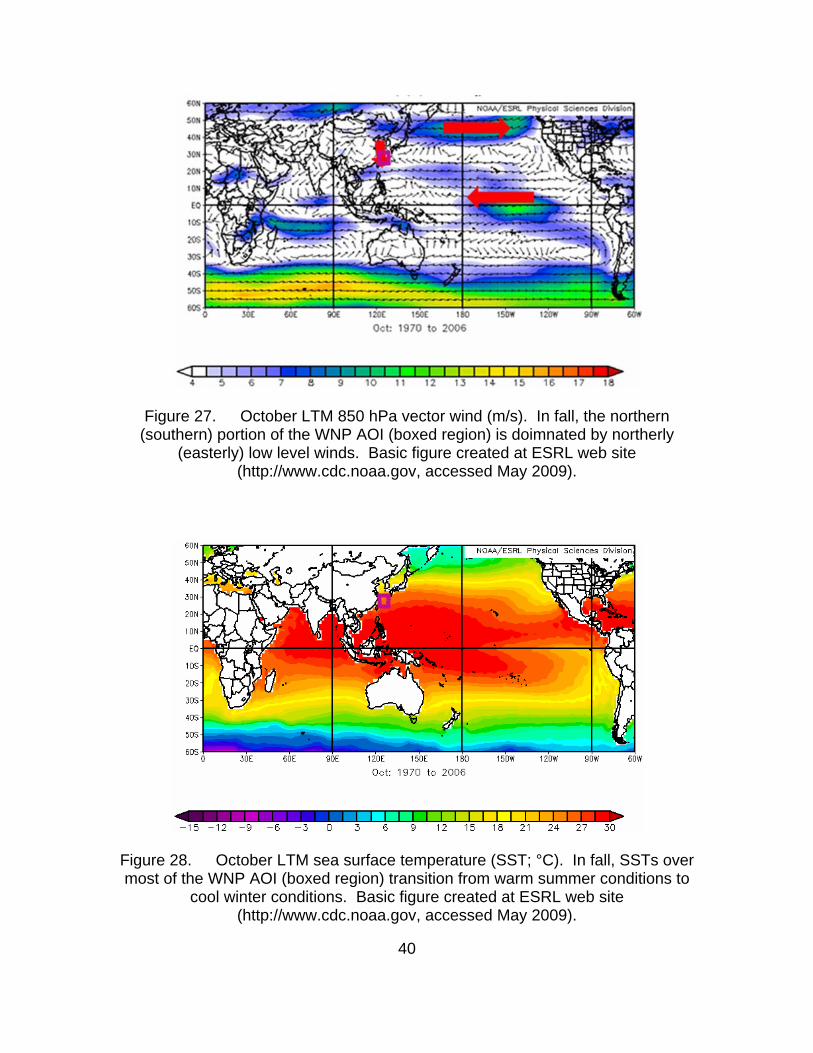
40

Figure 27. October LTM 850 hPa vector wind (m/s). In fall, the northern (southern) portion of the WNP AOI (boxed region) is doimnated by northerly

(easterly) low level winds. Basic figure created at ESRL web site (http://www.cdc.noaa.gov, accessed May 2009).

Figure 28. October LTM sea surface temperature (SST; °C). In fall, SSTs over most of the WNP AOI (boxed region) transition from warm summer conditions to

cool winter conditions. Basic figure created at ESRL web site (http://www.cdc.noaa.gov, accessed May 2009).

41

B. LONG TERM MEAN SEASONAL CYCLES: EDH AND FACTORS THAT DETERMINE EDH

We also examined the seasonal cycles of EDH and the factors that we

used to calculate EDH — air temperature at 2 meters, sea surface temperature,

wind speed at 10 meters, and relative humidity at 2 meters — with a focus on the

WNP in January, April, July, and October (Figures 29-44). See Chapter I,

sections C and D, to review the relationships between EDH and these factors.

1. January

Figure 29 shows the January LTM EDH for the WNP AOI. The overall

patterns are: (a) lower EDH close to the cool dry continent, over the East China

Sea (ECS) and South China Sea (SCS) where could dry winds flowing

southward away from the Asian High occur, and over colder ocean surfaces in

the northern part of the AOI; and (b) higher EDH over warmer ocean surfaces in

the southern part of the AOI (cf. Figures 11-16, 29-32). These patterns are

consistent overall with the general tendency for high SSTs, cool air, negative

ASTD, low relative humidity, and low wind speeds to lead to higher EDHs, and

vice versa. For example, note the broad correspondence between low (high)

ASTD and low (high) EDH (Figures 29 and 31). For most of the AOI in January,

the ASTD is negative, due to the flow of cold continental air over relatively warm

SSTs. Thus, we would expect the NPS bulk model to perform relatively well in

determining EDHs (see Chapter I, sections C and D).

42

Figure 29. January LTM EDH (m) for the WNP AOI.

Figure 30. January LTM wind speed (m/s) at 10 meters for WNP AOI.

43

Figure 31. January LTM air-sea temperature difference (°C) for WNP AOI.

Figure 32. January LTM relative humidity (%) at 2 meters for WNP AOI.

44

2. April

Figures 33-36 show the April LTM EDH and associated factors. Almost all

of the AOI has lower EDHs in April than in January (Figure 33). The main

exception is the southern Sea of Japan where the increased EDHs may be

attributable to a decrease in humidity and a change from unstable to near-neutral

conditions (Figures 35-36). More moisture is present in April than in January

over most of the southern ocean region in the AOI (Figure 36), leading to a

decrease in the EDH over most of this region compared to January. The EDH

maxima over the northeastern portion of the Yellow Sea should be regarded with

caution, since it is: (a) associated with strongly positive ASTD and EDH is very

sensitivity to ASTD when ASTD is positive; and (b) surrounded on several sides

by land and thus may be overly influenced by conditions over the land (see

Chapter II, section B).

Figure 33. April LTM EDH (m) for the WNP AOI.

45

Figure 34. April LTM wind speed (m/s) at 10 meters for WNP AOI.

Figure 35. April LTM air-sea temperature difference (°C) for WNP AOI.

46

Figure 36. April LTM relative humidity (%) at 2 meters for WNP AOI.

3. July

In July, the WNP AOI is dominated by that the northward advection warm,

moist air by relatively weak winds from the tropics (see Figures 21-24, 38, 40).

The higher relative humidity combined with near-neutral and weakly stable

conditions lead to lower EDHs in the northern latitudes compared to April (Figure

37). Conversely, the lower relative humidity and weakly unstable conditions in

the southern latitudes (south of roughly 30°N; Figures 39-40) combine to produce

higher EDHs than in April.

47

Figure 37. July LTM EDH (m) for the WNP AOI.

Figure 38. July LTM wind speed (m/s) at 10 meters for WNP AOI.

48

Figure 39. July LTM air-sea temperature difference (°C) for WNP AOI.

Figure 40. July LTM relative humidity (%) at 2 meters for WNP AOI.

4. October

Figures 41-44 show the October LTM EDH and associated factors. The

overall patterns in EDH are broadly similar to those for July, but the range of

49

EDH values in October is smaller than in July (compare Figures 37, 41). The

EDH (Figure 41) shows the influence of the weakening and eastward shift of the

North Pacific High, the development of the Asian High, and the onset of strong

southward outflows of cold dry air from East Asia and over the Yellow Sea, ECS,

and SCS (Figures 25-28, 42, 44). During October, the entire AOI is unstable

(negative ASTD, Figure 43). These changes result in increased EDHs in all but

the most southern portions (south of roughly 20° N) of the region of interest

compared to July (compare Figures 37, 41).

Figure 41. October LTM EDH (m) for the WNP AOI.

50

Figure 42. October LTM wind speed (m/s) at 10 meters for WNP AOI.

Figure 43. October LTM air-sea temperature difference (°C) for WNP AOI.

51

Figure 44. October LTM relative humidity (%) at 2 meters for WNP AOI.

C. LONG TERM MEAN SEASONAL CYCLES: RADAR DETECTION RANGES

To investigate the seasonal cycle of radar detection range in the WNP AOI

in an unclassified context, we worked with a generic surface search radar with

realistic parameters. This generic radar has a frequency of 9 GHz, is positioned

85 feet above the ocean surface, and is searching for a small target located four

feet above the ocean surface and with a detection threshold of 150 dB. The

process for calculating RDR is based on the calculation of EDH (see Chapter II,

section B). Since RDR is derived from and closely related to EDH, the seasonal

cycle of RDR is similar to that of EDH.

Figures 45-48 show the January, April, July, and October LTM RDRs, for

the WNP AOI. Note: (a) the general correspondence between high (low) EDH

and long (short) RDR (compare Figures 29, 33, 37, and 41 to Figures 45-48); (b)

the differences in RDR within the AOI for a given month (e.g., differences on the

order of 10 nmi between the Sea of Japan and the Kuroshio region south of

Japan in January); and (c) the differences in RDR between months for a given

52

location within the AOI (e.g., differences on the order of 10 nmi between January

and July for the Sea of Japan and the Kuroshio region south of Japan).

The RDR maps shown in Figures 45-48 provide useful guidance for

military planners on: (a) the ability to detect adversaries and be detected by

adversaries; and (b) managing the opportunities and risks posed by those

abilities. However, this guidance is based on long term mean (LTM) conditions

and does not account for the climate variations (deviations from LTM conditions)

that are known to occur in the WNP (e.g., Figure 5; Ford 2000; Tournay 2007;

Turek 2008; Mundhenk 2009). Thus, the RDR differences between locations and

between months discussed in the preceding paragraph very likely under-state the

spatial and temporal differences that actually occur in the WNP. The impacts of

these climate variations on EDH and RDR are discussed in the following section.

Figure 45. January LTM RDR (nmi) for WNP AOI.

53

Figure 46. April LTM RDR (nmi) for WNP AOI.

Figure 47. July LTM RDR (nmi) for WNP AOI.

54

Figure 48. October LTM RDR (nmi) for WNP AOI.

D. OCTOBER CONDITIONAL COMPOSITES

1. Conditional Composites Based on Winds

Wind is a large factor in directly and indirectly determining EDH (see

Chapter II, section B.3). Turek (2008) showed that large meridional wind

variations occur in the WNP during October and are associated with large

variations in SST and implied variations in low level air temperature and relative

humidity. We investigated the impacts of these variations by identifying Octobers

during 1970-2006 that experienced high and low meridional monthly mean winds

in a region east of Taiwan bounded by 20-28°N and 123-128°E (Figures 9, 49-

52). We then created conditional composites of meridional wind, EDH, and RDR

for the years with the five highest and lowest October mean meridional wind

speeds. These conditional composites were then compared and analyzed to see

how the variations in the magnitude of the wind, EDH, and RDR are related

during high and low wind years.

55

Figures 49-52 from Turek (2008) show the conditional composite winds

and wind anomalies for the October high wind and low wind years. The

composites indicate that the high (low) winds are associated with an early (late)

transition to winter conditions in the ECS, SCS, and Ryuku Islands regions (see

Figures 25-28, 41-44). This is especially evident in the anomalies (Figures 51-

52) which in these regions show anomalously strong (weak) northeasterly winds

in the high (low) wind composite. The conditional composites of the five

Octobers during 1970-2006 with the highest (longest) and lowest (shortest)

monthly mean EDH (RDR) in the region east of Taiwan bounded by 20-28°N and

123-128°E are shown in Appendix A. The wind, EDH, and RDR conditional

composites are useful indicators of the extremes that planners may need to

prepare for when operating in the WNP. However, conditional composites do not

by themselves indicate the conditions that are most likely for a given period in the

future (e.g., for an upcoming October). But the likely conditions can be

determined from a long range forecasts (LRFs) generated using information

about the past occurrences represented by conditional composites — for

example, LRFs that use data from past occurrences of high wind events to

predict future high wind events.

56

Figure 49. October conditional composite of surface winds for the five years with the highest meridional wind speeds avearged over 20-28°N, 123-128°E

(area east of Taiwan shown in Figure 9). From Turek (2008).

Figure 50. October conditional composite of surface winds for the five years with the lowest meridional wind speeds avearged over 20-28°N, 123-128°E (area

east of Taiwan shown in Figure 9). From Turek (2008).

57

Figure 51. October conditional composite anomaly of surface winds for the five years with the highest meridional wind speeds avearged over 20-28°N, 123-

128°E (area east of Taiwan shown in Figure 9). From Turek (2008).

Figure 52. October conditional composite anomaly of surface winds for the five years with the lowest meridional wind speeds avearged over 20-28°N, 123-128°E

(area east of Taiwan shown in Figure 9). From Turek (2008).

58

E. DEVELOPMENT OF LONG RANGE FORECAST PROCESS

U. S. Navy planners often begin preparing for an operation or exercise at

lead times of up to four months and their decisions can benefit greatly by having

accurate long range guidance on the expected environmental conditions and the

resulting impacts on sensor and weapons systems performance. The statistical

long range forecast methods used in this study require reliable predictors. We

experimented with using indices of El Nino – La Nina (ENLN) as predictors but

found relatively low correlations with our predictands, meridional wind, EDH,

RDR in our WNP AOI focus region east of Taiwan (see Figure 9). So we then

searched for other potential predictors by correlating the predictands with

numerous atmospheric and oceanic variables. We found that all three

predictands were well correlated with equatorial SST near the dateline (in the

western half of the Nino 4.0 box, 5°S-5°N, 160°E-175°W) when the SST lead the

predictands by zero to five months. This indicated that this SST could be a

useful long range predictor. Prior studies indicate that this SST is a physically

plausible predictor and likely influences the WNP AOI by altering equatorial

Pacific atmospheric convection, which leads to anomalous Rossby wave activity

that then alters the circulation in the WNP AOI (e.g., Ford 2000; Tournay 2007).

Figures 55-59 show maps of the correlations for 1970-2006 of monthly

mean October RDR in the focus region east of Taiwan (purple box) with global

monthly mean SST, with SST leading by zero to four months. Correlation

magnitudes of 0.318 or greater indicate significance at the 95% confidence level

(see Chapter II, section B.2). The red box on the equator near the dateline in

each correlation map indicates a region of high correlation at all lead times (e.g.,

correlations with October RDRs in the WNP focus region of 0.60, 0.55, 0.50,

0.50, and 0.35 for SST in October, September, August, July, and June,

respectively).

Figures 53-57 show broad scale correlation patterns that are similar to

SST anomaly patterns for ENLN (e.g., Ford 2000; Schwing et al. 2002). This

59

suggests that the processes that cause climate variations in the WNP, including

RDR variations, are physically plausible and related to ENLN — for example, that

EN (LN) related positive SST anomalies in the central and eastern equatorial

Pacific during June-October tend to be associated with positive (negative) RDR

anomalies in the WNP in October. However, the details of the correlation

patterns indicate that the relationship to ENLN is strongest for equatorial SSTs

near the dateline (red box in Figures 53-57), on the far western edge of the

central and eastern equatorial Pacific region where EN and LN related SST

anomalies tend to be strongest. So the relationships to ENLN are notable but not

especially robust.

Similar maps (not shown) were constructed for correlations between

meridional wind and EDH in the WNP focus region with SST, and for correlations

of all three WNP predictands with other potential predictors (e.g., air temperature,

geopotential height, etc.). However, the correlations with the equatorial SST

near the dateline tended were the highest overall for zero to four-month lead

times. All the correlations had similar spatial patterns and were physically

consistent (e.g., SST was positively (negatively) correlated with RDR and EDH

and high (low) wind speeds). These results support the conclusion that the

correlations are physically plausible and represent real physical processes.

60

Figure 53. Correlation of October radar detection range (RDR) in the focus region east of Taiwan (purple box) with SST in October for the years 1970-2006. The RDR is for a 9 GHz radar at 85 ft above the surface, looking for a 4 ft target

with a detection threshold of 150 dB. The red box highlights a region of persistently high correlations when SST leads October RDR by zero to five

months (see Figures 55-59). Basic figure created at ESRL web site (http://www.cdc.noaa.gov, accessed May 2009).

61

Figure 54. Correlation of October radar detection range (RDR) in the focus region east of Taiwan (purple box) with SST in September for the years 1970-

2006. The RDR is for a 9 GHz radar at 85 ft above the surface, looking for a 4 ft target with a detection threshold of 150 dB. The red box highlights a region of

persistently high correlations when SST leads October RDR by zero to five months (see Figures 55-59). Basic figure created at ESRL web site

(http://www.cdc.noaa.gov, accessed May 2009).

62

Figure 55. Correlation of October radar detection range (RDR) in the focus region east of Taiwan (purple box) with SST in August for the years 1970-2006. The RDR is for a 9 GHz radar at 85 ft above the surface, looking for a 4 ft target

with a detection threshold of 150 dB. The red box highlights a region of persistently high correlations when SST leads October RDR by zero to five

months (see Figures 55-59). Basic figure created at ESRL web site (http://www.cdc.noaa.gov, accessed May 2009).

63

Figure 56. Correlation of October radar detection range (RDR) in the focus region east of Taiwan (purple box) with SST in July for the years 1970-2006.

The RDR is for a 9 GHz radar at 85 ft above the surface, looking for a 4 ft target with a detection threshold of 150 dB. The red box highlights a region of



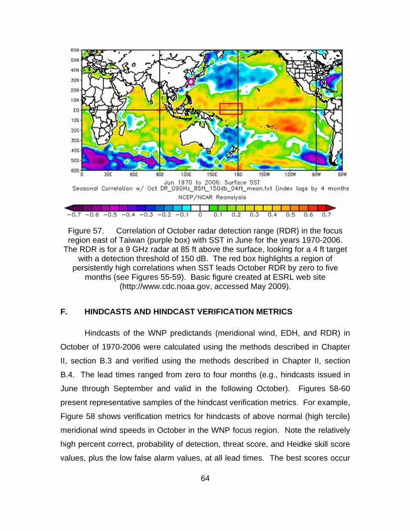
64

Figure 57. Correlation of October radar detection range (RDR) in the focus region east of Taiwan (purple box) with SST in June for the years 1970-2006.

The RDR is for a 9 GHz radar at 85 ft above the surface, looking for a 4 ft target with a detection threshold of 150 dB. The red box highlights a region of



F. HINDCASTS AND HINDCAST VERIFICATION METRICS

Hindcasts of the WNP predictands (meridional wind, EDH, and RDR) in

October of 1970-2006 were calculated using the methods described in Chapter

II, section B.3 and verified using the methods described in Chapter II, section

B.4. The lead times ranged from zero to four months (e.g., hindcasts issued in

June through September and valid in the following October). Figures 58-60

present representative samples of the hindcast verification metrics. For example,

Figure 58 shows verification metrics for hindcasts of above normal (high tercile)

meridional wind speeds in October in the WNP focus region. Note the relatively

high percent correct, probability of detection, threat score, and Heidke skill score

values, plus the low false alarm values, at all lead times. The best scores occur

65

at one month lead times, perhaps because lags in the dynamical processes that

links the SST predictor to the meridonal wind predictand mean that the link is

less apparent when there is no lag (i.e., when the lead time is zero). This relative

high scores at the longer lead times is clear evidence that skillful long range

forecasts of WNP meridional winds, and the closely related EDH and RDR, could

be made up to lead times of 5 months with greater skill than that of traditional

climatology.

Figure 58. Verification metrics for hindcasts for 1970-2006 of above normal (i.e., high) meridonal wind in October in the WNP focus region using eqatorial SST near the dateline in October, September, August, July, and June as the

predictor. The hindcast methods, and the metrics and metrics legend acronyms are explained in Chapter II, section B. See text for additonal details.

66

Figure 59. Verification metrics for hindcasts for 1970-2006 of above normal (i.e., high) EDH in October in the WNP focus region using eqatorial SST near the

dateline in October, September, August, July, and June as the predictor. The hindcast methods, and the metrics and metrics legend acronyms are explained in

Chapter II, section B. See text for additonal details.

Figure 60. Verification metrics for hindcasts for 1970-2006 of near normal RDR in October in the WNP focus region using eqatorial SST near the dateline in

October, September, August, July, and June as the predictor. The hindcast methods, and the metrics and metrics legend acronyms are explained in Chapter

II, section B. See text for additonal details.

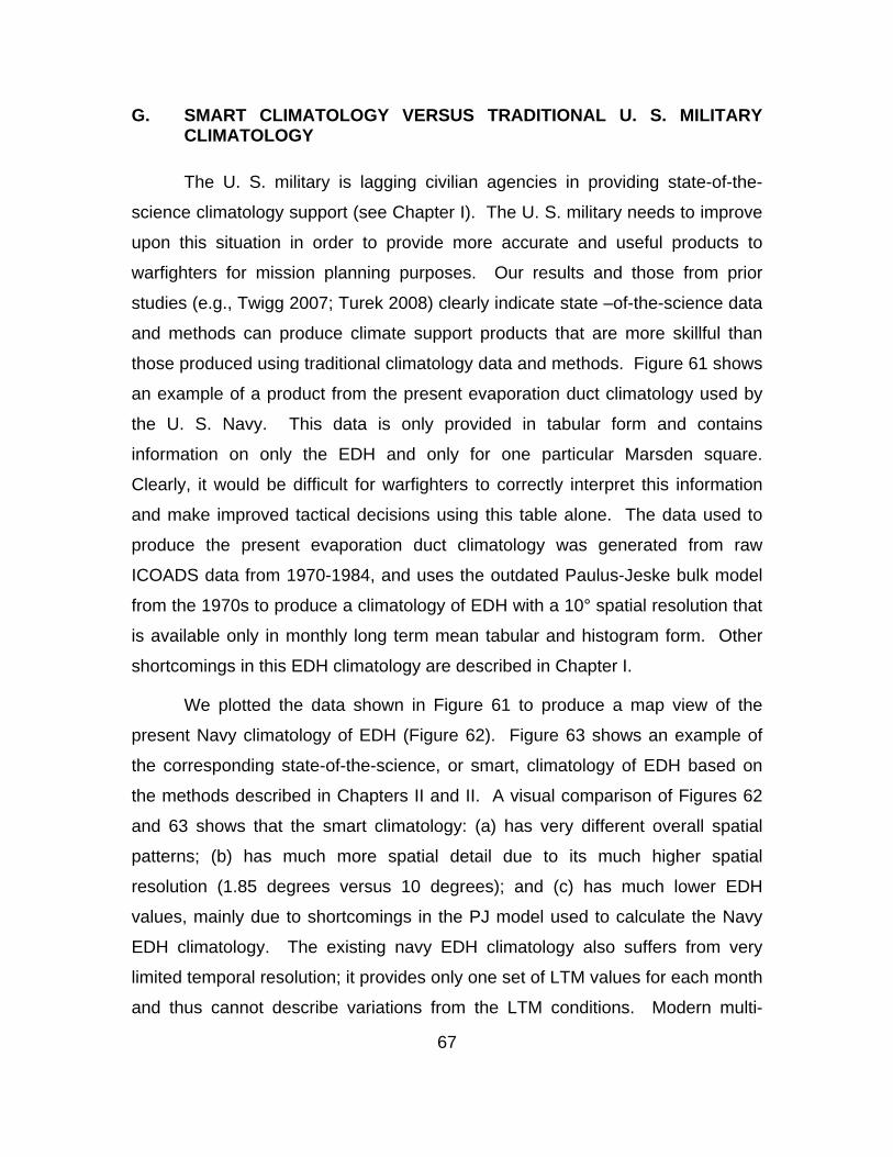
67

G. SMART CLIMATOLOGY VERSUS TRADITIONAL U. S. MILITARY CLIMATOLOGY

The U. S. military is lagging civilian agencies in providing state-of-the-

science climatology support (see Chapter I). The U. S. military needs to improve

upon this situation in order to provide more accurate and useful products to

warfighters for mission planning purposes. Our results and those from prior

studies (e.g., Twigg 2007; Turek 2008) clearly indicate state –of-the-science data

and methods can produce climate support products that are more skillful than

those produced using traditional climatology data and methods. Figure 61 shows

an example of a product from the present evaporation duct climatology used by

the U. S. Navy. This data is only provided in tabular form and contains

information on only the EDH and only for one particular Marsden square.

Clearly, it would be difficult for warfighters to correctly interpret this information

and make improved tactical decisions using this table alone. The data used to

produce the present evaporation duct climatology was generated from raw

ICOADS data from 1970-1984, and uses the outdated Paulus-Jeske bulk model

from the 1970s to produce a climatology of EDH with a 10° spatial resolution that

is available only in monthly long term mean tabular and histogram form. Other

shortcomings in this EDH climatology are described in Chapter I.

We plotted the data shown in Figure 61 to produce a map view of the

present Navy climatology of EDH (Figure 62). Figure 63 shows an example of

the corresponding state-of-the-science, or smart, climatology of EDH based on

the methods described in Chapters II and II. A visual comparison of Figures 62

and 63 shows that the smart climatology: (a) has very different overall spatial

patterns; (b) has much more spatial detail due to its much higher spatial

resolution (1.85 degrees versus 10 degrees); and (c) has much lower EDH

values, mainly due to shortcomings in the PJ model used to calculate the Navy

EDH climatology. The existing navy EDH climatology also suffers from very

limited temporal resolution; it provides only one set of LTM values for each month

and thus cannot describe variations from the LTM conditions. Modern multi-

68

decadal reanalysis data sets provide much higher temporal resolution and the

ability to develop LRF products such as those described in Chapter III, sections

D-F).

Figure 61. October LTM evaporation duct height (EDH) example of the present U. S. Navy LTM EDH climatology in tabular format.

69

Figure 62. October LTM evaporation duct height (EDH) example of the present U. S. Navy LTM EDH climatology, after we manually entered and then

plotted the data shown in Figure 61.

Figure 63. October LTM evaporation duct height (EDH) example of applying modern climate data sets and methods to develop a state-of-the-science EDH climatology. Note the large differences between this modern EDH climatology

and the present Navy climatology (Figure 61-62).

70

These comparisons are just some of the many examples of how existing

military climatologies fall well short of the accuracy, spatial and temporal

resolutions, predictive capabilities, and usability that are possible using modern

climatology data sets and methods. When the U. S. military decides to seriously

pursue the development and production of modern climate analyses and long

range forecasts, then warfighters will begin receiving the long lead support they

need — for example, the best available long lead radar performance predictions.

H. LONG RANGE FORECASTS OF EDH AND RDR

We applied our long range forecasting methodology (see Chapter II,

section B), and the lessons learned from our hindcasts (see Chapter III, section

F) to produce long range forecasts (LRFs) of the evaporation duct height and

radar detection ranges in the WNP for November 2009. These LRFs are

classified and can be found in the classified Appendix B of this thesis. This

appendix is available in the classified section of the Dudley Knox Library of the

Naval Postgraduate School in Monterey, California.

71

IV. SUMMARY, CONCLUSIONS, AND RECOMMENDATIONS

A. SUMMARY AND CONCLUSIONS

We developed and tested a method for producing long range forecasts

(LRFs) of winds, evaporation duct height, and radar detection range in the

western North Pacific (WNP). The method shows a high potential for producing

skillful operational LRFs that would significantly improve long lead support for the

planning of military operations in the WNP. In particular, such support would

have important applications in planning naval operations such as radar detection

and tracking of submarine periscopes, low-flying missiles and aircraft, and

surface combatants. We provided examples of the use of state-of-the-science

data sets and methods for developing more accurate and useful climatologies,

climate analyses, and LRFs of atmospheric electromagnetic propagation and

radar performance for the WNP and with a focus on October. But the same

basic data sets and methods can be used for many other climate and operational

variables (e.g., sonic layer depth and sonar detection ranges), other locations,

and other periods. We also created classified long range forecasts of

environmental conditions and radar performance in the WNP in November 2009.

These LRFs were developed to support the planning of naval operations that will

be conducted in November 2009. The LRFs will be verified in early 2010. These

LRFs can be found in the classified section of the Dudley Knox Library at the

Naval Postgraduate School located in Monterey, CA.

One of several limitations of our research is that in some coastal locations

the reanalysis data used to represent conditions over the ocean may be overly

influenced by data from land locations (see Chapter II, section B.1). Thus, EDH

and RDR results for such locations points should be viewed with caution. One

additional limitation is that our radar detection ranges are based only on the

72

evaporation duct and do not account for surface-based ducts. The operational

significance of this shortcoming and methods for correcting it need to be studied

in the future.

B. RECOMMENDATIONS FOR FUTURE RESEARCH

We recommend that research similar to ours be conducted in the near

future when higher resolution reanalysis data sets become available. A

reanalysis data set with higher horizontal and vertical resolution would: (a)

reduce the coastal problems discussed in Chapter II, section B.1; and (b) provide

an increased number of levels below 700 mb which would allow for better

mapping of both surface based ducts and evaporation ducts. By the end of

2009, NCEP is expected to release a global coupled atmospheric-oceanic

reanalysis with a 0.25° by 0.25° horizontal resolution for the ocean and 0.5° by

0.5° horizontal resolution for the atmosphere. We recommend that future

research investigate the use of this and other forthcoming higher resolution

reanalysis data sets.

Predictors were selected by computing correlations between potential

predictors and the predictands. We used sea surface temperatures as our

predictor, but additional potential predictors and sets of predictors should be

researched in the future. In addition, other statistical and statistical-dynamical

LRF methods should be investigated, such as the composite analysis forecasting

method (Hanson 2007; Moss 2007).

Future research should investigate methods for producing independent

data sets for verifying reanalysis variables, and analyses and LRFs of EDH and

RDR. This might be accomplished using long term buoy observations (cf. Twigg

2007) or analyses of ducts and radar performance based on field experiments in

the WNP.

Smart climatology for military applications is presently done mainly by

DoD climate researchers. Their prototype operational products should be

73

applied in future research and development efforts to test these products in

operational planning and to assess the value of those products to the military

planning process.

74


75

APPENDIX

Figure 64. February LTM EDH (m) for the WNP AOI.

Figure 65. March LTM EDH (m) for the WNP AOI.

76

Figure 66. May LTM EDH (m) for the WNP AOI.

Figure 67. June LTM EDH (m) for the WNP AOI.

77

Figure 68. August LTM EDH (m) for the WNP AOI.

Figure 69. September LTM EDH (m) for the WNP AOI.

78

Figure 70. November LTM EDH (m) for the WNP AOI.

Figure 71. December LTM EDH (m) for the WNP AOI.

79

Figure 72. February LTM RDR (nmi) for WNP AOI.

Figure 73. March LTM RDR (nmi) for WNP AOI.

80

Figure 74. May LTM RDR (nmi) for WNP AOI.

Figure 75. June LTM RDR (nmi) for WNP AOI.

81

Figure 76. August LTM RDR (nmi) for WNP AOI.

Figure 77. September LTM RDR (nmi) for WNP AOI.

82

Figure 78. November LTM RDR (nmi) for WNP AOI.

Figure 79. December LTM RDR (nmi) for WNP AOI.

83

Figure 80. October conditional composite based on the five shortest RDR years of a generic radar.

Figure 81. October conditional composite based on the five longest RDR years of a generic radar.

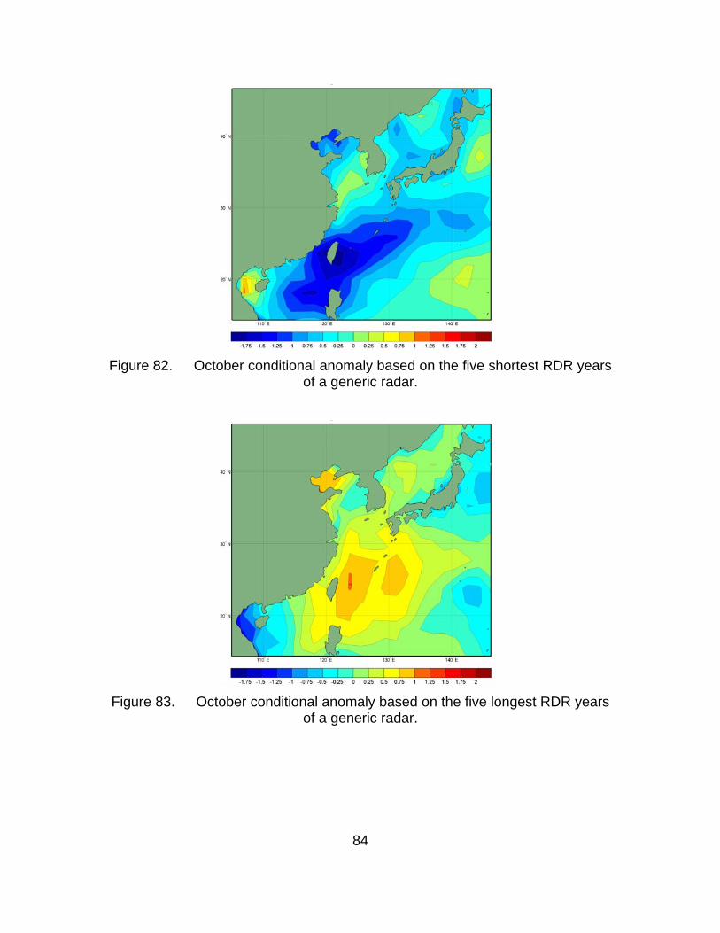
84

Figure 82. October conditional anomaly based on the five shortest RDR years of a generic radar.

Figure 83. October conditional anomaly based on the five longest RDR years of a generic radar.

85

Figure 84. October LTM of RDR (nmi) for a generic radar.

Figure 85. October conditional composite based on the five lowest EDH years.

86

Figure 86. October conditional composite based on the five highest EDH

years.

Figure 87. October conditional anomaly based on the five lowest EDH years.

87

Figure 88. October conditional anomaly based on the five highest EDH years.

88


89

LIST OF REFERENCES

Babin, S. M., G. S. Young, and J. A. Carton, 1997: A new model of the oceanic evaporation duct. Journal of Applied Meteorology, Boston, MA, 36, 193-204.

Barrios, A. E., W. L. Patterson, 2002: Advanced propagation model (APM) ver

1.3.1 computer software configuration item (CSCI) documents. SPAWAR Systems Center, San Diego, Tech. Doc. 3145, 479 pp.

Bean, B. R., and E. J. Dutton, 1968: Radio Meteorology. Dover Publications,

New York, 435 pp. Bjerkness, J., 1966: A possible response of the atmospheric Hadley circulation

to equatorial anomalies of ocean temperature. Tellus, 18, 820-829. ———. 1969: Atmospheric teleconnections from the equatorial Pacific. Mon.

Wea. Rev., 97, 163-172. ———. 1972: Large-scale atmospheric response to the 1964-1965 Pacific

equatorial warming. J. Phys. Oceanogr., 2, 212-217. Finley, J. P., 1884: Tornado predictions. Amer. Meteor. J., 1, 85–88. Ford, B. W., 2000: El Nino and La Nina effects on tropical cyclones: the

mechanisms. M. S. thesis, Dept. of Meteorology, Naval Postgraduate School, 190 pp.

Frederickson, P. A., K. L. Davidson, and A. K. Goroch, 2000: Operational bulk

evaporation duct model for MORIAH, Version1.2. Naval Postgraduate School, 70 pp. (Available from P. A. Frederickson, Naval Postgraduate School, 589 Dyer Road, Monterey, CA 93943-5114).

Frederickson, P. A., and K. L. Davidson, 2008: Operational bulk evaporation duct

model. Naval Postgraduate School, 55 pp. (Available from P. A. Frederickson, Naval Postgraduate School, 589 Dyer Road, Monterey, CA 93943-5114).

Frederickson, P., and T. Murphree, 2008: “A Modern Global Evaporation Duct

Climatology,” RADAR Conference, Adelaide, South Australia, 04 September 2008.

90

Hanson, C. M., 2007: Long-range operational military forecasts for Iraq. Master’s thesis, Dept. of Meteorology, Naval Postgraduate School, Monterey, California, 59 pp.

Heidt, S., 2009: Long-range atmosphere-ocean forecasting in support of USW

operations in the western North Pacific. Master’s thesis, Dept. of Meteorology, Naval Postgraduate School, Monterey, California.

Hendon, H. H., and M. L. Salby, 1994: The life cycle of the Madden and Julian

oscillation. J. Atmos. Sci., 51, 2225–2237. Kalnay, E., M. Kanamitsu, R. Kistler, W. Collins, D. Deaven, L. Gandin, M.

Iredell, S. Saha, G. White, J. Woollen, Y. Zhu, A. Leetmaa, R. Reynolds, M. Chelliah, W. Ebisuzaki, W. Higgins, J. Janowiak, K. Mo, C. Ropelewski, J. Wang, R. Jenne, and D. Joseph, 1996: The NCEP/NCAR 40-year Reanalysis Project. Bull. Amer. Meteor.Soc., 77, 437-471.

Kistler, R., E. Kalnay, W. Collins, S. Saha, G. White, J. White, J. Woollen, M.

Chelliah, W. Ebisuzaki, M. Kannamitsu, V. Kousky, H. van den Dool, R. Jenne, and M. Fiorino, 2001: The NCEP/NCAR 50-year Reanalysis: Monthlymeans CD-ROM and documentation. Bull. Amer. Meteor. Soc., 82, 247-267.

LaJoie, M., 2006: The impact of climate variations on military operations in the

Horn of Africa. Master’s. thesis, Dept. of Meteorology, Naval Postgraduate School, Monterey, California, 131 pp.

Mathworks, 2008: MATLAB 7.7, The MathWorks, Inc.

Molg, T., M. Renold, M. Vuille, N. J. Cullen, T. F. Stocker, and G. Kaser, 2006: Indian Ocean zonal mode activity in a multicentury-integration of a coupled AOGCM consistent with climate proxy data, Geophys. Res. Lett., doi:10.1029/2006GL026384, in press.

Montgomery, C., 2008: Climate variations in tropical West Africa

and their implications for military planners. Master’s thesis, Dept. of Meteorology, Naval Postgraduate School, 89 pp.

Moss, S. M., 2007: Long-range operational military forecasts for Afghanistan.

Department of Meteorology, Naval Postgraduate School, Monterey, California. 77pp.

Mundhenk, B. D., 2009: A statistical-dynamical approach to intraseasonal

prediction of tropical cyclogensis in the western North Pacific. M. S. thesis, Dept. of Meteorology, Naval Postgraduate School, Monterey, California, 107 pp.

91

Murphree, T., 2008a: MR3610 Course Module 6: Smart Climatology. Department of Meteorology, Naval Postgraduate School, Monterey, California, 52 pp.

Murphree, T., 2008b: MR3610 Course Module 19: Madden-Julian Oscillation Part 1. Department of Meteorology, Naval Postgraduate School, Monterey, California, 32 pp.

Rasmusson, E. G., and T. H. Carpenter, 1982: Variations in tropical sea surface temperature and surface wind fields associated with the Southern Oscillation/El Nino. Mon Wea. rev., 110, 354-384.

Patterson, W. L., 1987: Historical Electromagnetic Propagation Condition Database Description, Naval Oceans Systems Center, San Diego, California. NOSC TD 1149.

Saji, N. H., B. N. Goswami, P. N. Vinayachandran, and T. Yamagata, 1999: A dipole mode in the tropical Indian Ocean. Nature, London, England, 401, 360-363.

Saji, N. H., T. Yamagata, 2003: Possible impacts of Indian Ocean Dipole mode events on global climate. Clim.Res., 25, 151-169.

Schwing, F., T. Murphree, L. deWitt, and P. Green, 2002: The evolution of oceanic and atmospheric anomalies in the northeast Pacific during the El Niño and La Niña events of 1995-2001. Progress in Oceanography, 54, 459-491.

Tournay, R. C., 2008: Long-range statistical forecasting of Korean summer precipitation. Master’s thesis, Dept. of Meteorology, Naval Postgraduate School, Monterey, California, 121pp.

Turek, A., 2008: Smart climatology applications for undersea warfare. M. S. thesis, Dept. of Meteorology, Naval Postgraduate School, Monterey, California, 95 pp.

Twigg, K. L., 2007: A smart climatology of evaporation duct height and surface radar propagation in the Indian Ocean. M. S. thesis, Dept. of Meteorology, Naval Postgraduate School, Monterey, California, 135 pp.

Walker, G., 1924: Correlation in seasonal variations of weather IX: A further weather study of world weather. Memoirs of the Royal Meteorological Society, 24, 275-322.

Walker, G., and E. Bliss, 1932: World Weather V. Memoirs of the Royal Meteorological Society, 4, 53-84.

92

Webster, P. J., A. M. Moore, J. P. Loschnigg, and R. R. Leben, 1999: Coupled ocean-atmosphere dynamics in the Indian Ocean during 1997-98. Nature, London, England, 401, 356-360.

Wilks, D. S., 2006: Statistical Methods in the Atmospheric Sciences. 2nd ed. Academic Press, 627 pp.

Wolter, K., and M.S. Timlin, 1993: Monitoring ENSO in COADS with a seasonally adjusted principal component index. Proc. of the 17th Climate Diagnostics Workshop, Norman, OK, NOAA/N MC/CAC, NSSL, Oklahoma Clim. Survey, CIMMS and the School of Meteor., Univ. of Oklahoma, 52-57.

Wolter, K., and M. S. Timlin, 1998: Measuring the strength of ENSO events — how does 1997/98 rank? Weather, 53, 315-324.

93

INITIAL DISTRIBUTION LIST

1. Defense Technical Information Center Ft. Belvoir, Virginia

2. Dudley Knox Library Naval Postgraduate School Monterey, California

3. Dr. Tom Murphree Meteorology Department, Code MR/Me Naval Postgraduate School Monterey, California

4. Mr. Paul Frederickson Meteorology Department, Code MR/Fd Naval Postgraduate School Monterey, California

naval postgraduate school naval postgraduate school ... the ability to predict the evaporation duct...

Documents