Nature or Nurture:

What Determines Investor Behavior?∗

Amir Barnea, Henrik Cronqvist, and Stephan Siegel†

First version: July 9, 2009This version: February 3, 2010

Abstract

Using data on identical and fraternal twins’ complete financial portfolios, we decompose the cross-sectional variation in investor behavior. We find that a genetic factor explains about one thirdof the variance in stock market participation and asset allocation. Family environment has aneffect on the behavior of young individuals, but this effect is not long-lasting and disappearsas an individual gains experiences. Frequent contact among twins results in similar investmentbehavior beyond a genetic factor. Twins who grew up in different environments still displaysimilar investment behavior. Our interpretation of a genetic component of the decision to in-vest in the stock market is that there are innate differences in factors affecting effective stockmarket participation costs. We attribute the genetic component of asset allocation - the relativeamount invested in equities and the portfolio volatility - to genetic variation in risk preferences.

∗We thank two anonymous referees and seminar participants at the 2010 European Winter Finance Conference,Hebrew University, Tel-Aviv University, University of Arizona, University of British Columbia, University of Californiaat Riverside, University of Minnesota, and University of Washington, and John Boyd, Daniel Dorn, Adlai Fisher,Murray Frank, Todd Gormley, Greg Hess, Avi Kamara, Jon Karpoff, Harald Kullmann, David Mayers, Ed Rice,Richard Smith, Martin Weber, Ingrid Werner, Scott Yonker, and Paul Zak for valuable comments. We are thankfulto Jack Goldberg at the University of Washington Twin Registry for advice. We thank Statistics Sweden, theSwedish Twin Registry, the Swedish Investment Fund Association, Euroclear Sweden, and S&P for assistance withthe data. Hannah Gregg and Lew Thorson provided outstanding research assistance. We acknowledge generousresearch funding from the Financial Economics Institute and the Lowe Institute of Political Economy at ClaremontMcKenna College (Barnea and Cronqvist), and the Global Business Center and the CFO Forum at the University ofWashington (Siegel). The Swedish Twin Registry is supported by grants from the Swedish Research Council, theMinistry of Higher Education, AstraZeneca, and the National Institute of Health (grants AG08724, DK066134, andCA085739). This project was pursued in part when Cronqvist was visiting the Swedish Institute for Financial Research(SIFR), which he thanks for its hospitality. The project has been reviewed by the Swedish Twin Registry (submitted12/31/2007, approved 3/14/2008), the Ethics Review Board for the Stockholm region (submitted 10/24/2008, approved11/26/2008), and Statistics Sweden (submitted 11/20/2008, approved 3/3/2009). Any errors or omissions are our own.†Barnea: Claremont McKenna College, Robert Day School of Economics and Finance (amir.barnea@cmc.edu);

Cronqvist: Claremont McKenna College, Robert Day School of Economics and Finance (hcronqvist@cmc.edu); Siegel:University of Washington, Michael G. Foster School of Business (ss1110@u.washington.edu).

Nature or Nurture:

What Determines Investor Behavior?

Abstract

Using data on identical and fraternal twins’ complete financial portfolios, we decompose the cross-sectional variation in investor behavior. We find that a genetic factor explains about one third ofthe variance in stock market participation and asset allocation. Family environment has an effect onthe behavior of young individuals, but this effect is not long-lasting and disappears as an individualgains experiences. Frequent contact among twins results in similar investment behavior beyonda genetic factor. Twins who grew up in different environments still display similar investmentbehavior. Our interpretation of a genetic component of the decision to invest in the stock market isthat there are innate differences in factors affecting effective stock market participation costs. Weattribute the genetic component of asset allocation - the relative amount invested in equities andthe portfolio volatility - to genetic variation in risk preferences.

I Introduction

It is a well documented empirical fact in the finance literature that there is significant heterogeneity

across individuals in investment behaviors such as the decision to invest in the stock market and the

choice of asset allocation.1 Are individual investors genetically predisposed to certain behaviors and

born with a persistent set of abilities and preferences which affect their decisions in the financial

domain?2 Or is investment behavior to a significant extent shaped by environmental factors, such as

parenting or individual-specific experiences? These questions are fundamental for our understanding

of the behavior of individual investors, but existing research has so far not offered much systematic

evidence on them. In this paper, we seek to fill this void by estimating the extent to which “nature,”

i.e., genetic variation across individuals, versus “nurture” or other environmental treatments explain

the observed heterogeneity in investment decisions.

To decompose the variance of three important measures of investment behavior – stock market

participation, the relative amount invested in equities (share of equities) and portfolio volatility –

into genetic and environmental components, we examine identical and non-identical twins. The

intuition of our identification strategy is straightforward: if individuals who are more closely related

genetically (e.g., identical twins) tend to be more similar on measures of investment behavior, then

this is evidence for that behavior being, at least partially, caused by a genetic factor. Using data on

twins allows us to identify an unobservable genetic component and environmental components that

are either common (shared) or non-shared among twins.

Our data on 37,504 twins are from the Swedish Twin Registry, which maintains and manages

the world’s largest database of twins. Until the abolishment of the wealth tax in Sweden in 2006,

the law required all financial institutions to report information to the Swedish Tax Agency about

the assets an individual owned as of December 31 of that year. This allows us to compile a matched

data set of twins and their complete financial portfolios.

1See, e.g., Campbell (2006) and Curcuru et al. (2009) for recent and extensive reviews of the emerging field of“household finance” and, specifically, research on the cross-sectional variance in investment behavior.

2There is a long-standing view in economics that preferences are at least partly genetic (e.g., Robson (2001a)), andRobson (2001b) goes as far as stating that “[i]f preferences are significantly shaped by individual experiences, thechanges needed in economic theory are profound” (p. 901). For early work in economics from a biological viewpoint,see Hirshleifer (1977).

1

Our empirical evidence shows that about a third of the cross-sectional variation in stock market

participation and asset allocation decisions across individuals is explained by a genetic factor. We

also demonstrate that the genetic component does not disappear with age, is significant even among

twins who do not interact very frequently, and accounts for a significant proportion of the variance

also among pairs of twins who were reared apart. While our evidence implies that nature is an

important determinant of an individual’s investment behavior, we also document considerable

environmental influences. Our evidence indicates that environmental influences that contribute

to variation in investor behavior are those that make family members different, not similar. That

is, the non-shared environment tend to be much more important than the shared environment in

explaining differences in investment behaviors. The family environment has a significant effect on

the investment behavior of young individuals, but this effect is not long-lasting (unless the twins

stay in frequent contact) as we find that it disappears when an individual gains own experiences

relevant for decisions in the investment domain.

In a standard frictionless model of asset allocation, all individuals, no matter how risk averse

they are, should invest at least a fraction of their portfolio in equities. But participation costs can

cause non-participation among some individuals.3 As a result, our interpretation of a significant

genetic component of the decision to invest in the stock market is that there are individual-specific

innate differences in factors that affect the magnitude of effective stock market participation costs.

Controlling for wealth, educational achievement, and several background risk factors does not

change our finding. This suggests that additional, heritable characteristics (unobservable to us)

play an important role in explaining stock market participation. This is consistent with evidence in

finance that risk aversion, social interactions, trust, and most recently cognitive ability and even

height are associated with stock market participation, while long-standing research in behavioral

genetics has found that these characteristics have a significant genetic component. Our evidence

thus suggests that accounting for genetic variation should be helpful in understanding these findings

better.

Our paper also contributes to research on the determinants of variation in asset allocation (share

3Vissing-Jørgensen (2002b) shows that relatively small ongoing participation costs can explain the non-participationrate in the stock market.

2

in equity and portfolio volatility) across individuals. Standard models show that in a frictionless

market, differences in risk preferences and possibly in wealth (if risk aversion is a function of wealth)

are the main sources of cross-sectional variation in the share in equities (e.g., Samuelson (1969) and

Merton (1969)). Recently, financial economists have also examined the influence of life cycle effects

(Ameriks and Zeldes (2004)) and various background risk factors which are absent in a standard

model (e.g., Heaton and Lucas (2000), Rosen and Wu (2004)), and Love (2010)). However, the

explanatory power with respect to asset allocation of such observable factors is low. For example,

the adjusted R2 is only 2-3 percent in most asset allocation studies (for a recent example, see

Brunnermier and Nagel (2008)). Our evidence demonstrates that modeling a genetic component

significantly improves our ability to explain the variation in asset allocation across individuals.

Importantly, because we control for wealth as well as background risk factors commonly studied in

the literature, such as entrepreneurial activity, health status, and marital status, our interpretation

of the evidence is that genetic variation in risk preferences explains the genetic component of

individuals’ asset allocation decisions. Such an interpretation is consistent with recent experimental

evidence on genetically determined preferences for risk taking (e.g., Kuhnen and Chiao (2009) and

Cesarini et al. (2009a)).

The paper is organized as follows. Section II contains an overview of related research. Section

III describes the empirical research methodology we use to quantitatively decompose the variance

in investment behavior into genetic and environmental components. Section IV describes our data

on twins and their investment portfolio, and defines the variables of interest. Section V reports our

results and robustness checks, and Section VI contains further evidence and extensions. Section VII

discusses our evidence and implications, and Section VIII concludes.

II Overview of Related Research

The question of the relative importance of nature versus nurture in explaining investment behavior

is related to an extensive body of work in behavioral genetics and to recent studies in economics

and finance. In this section, we provide an overview of the results that have emerged so far from

these literatures.

3

A Genetics and Preferences for Risk Taking

Two recent twin studies which estimate the genetic component of individuals’ risk taking preferences

are Cesarini et al. (2009a) and Zyphur et al. (2009). Using experiments involving lottery choices

and questionnaires, they elicit subjects’ risk preferences and then use twin research methodology

to estimate genetic effects. They find evidence of a significant genetic component which partly

explains the heterogeneity in risk preferences. However, eliciting preferences for risk taking using

experiments is problematic and may not necessarily provide a reliable measure (Harrison et al.,

2007).4 Both studies also employ small samples that are subject to potential sample selection bias.

For example, in Cesarini et al. (2009a) 80 percent of the subjects are female twins who selected to

participate in an experiment session (both twins in a pair had to be able to attend the session) and

Zyphur et al. (2009) study only male twins. Our paper does not use an experimental approach, but

studies real investment behavior as revealed by individuals’ portfolio choices.

Our work is most closely related to an independent study of Swedish twins by Cesarini et al.

(2009b). However, the analysis and the data sets are different. First, we examine individuals’ overall

financial portfolios, while Cesarini et al. (2009b) study a subset of an individual’s portfolio: the

public retirement savings account created in the pension reform in Sweden in 2000. In these accounts,

individuals allocate 2.5%, up to a cap, of their annual labor income. The initial retirement savings

accounts were small, and individuals may not have devoted significant effort to choose optimal

portfolios, but were influenced by advertising by fund managers and the government (Cronqvist

and Thaler (2004)). Second, we study standard measures in financial economics, in particular stock

market participation and the share of financial assets invested in equities, while Cesarini et al.

(2009b) focus on return volatility.5 Finally, the investment opportunity sets available to investors are

different. In our data set, individuals have access to all direct and indirect holdings of assets traded

domestically and internationally. In Cesarini et al. (2009b), individuals can only choose a maximum

of five funds from a list of approximately 450 diversified mutual funds available to investors in the

4See Levitt and List (2007) for a general discussion of strengths of, and potential problems with, experimentalapproaches in economic research.

5The main measure in Cesarini et al. (2009b) is “Risk 1,” defined as “the average risk level of the funds invested inby the individual, with the risk of each fund measured as the (annualized) standard deviation of the monthly rate ofreturn over the previous three years” (p. 5).

4

recently introduced public retirement system. This potentially results in more measurement error

as some individuals cannot attain their preferred risk provided the constraints.

Our research is also related to a small but rapidly growing literature on gene-mapping and on the

neural foundations of financial risk-taking.6 Researchers in this field examine whether the presence

of specific gene(s) may explain differences in risk-taking behavior in the cross-section of individuals.

This work is motivated by recent studies which suggest that genes regulate specific “feel-good”

neurotransmitters, e.g., dopamine, and affect the processing of information about rewarding. Taking

more risk may result in more or longer-lasting production of these neurotransmitters depending on

an individual’s genetic composition. Thus, risk taking may be experienced as more rewarding by

individuals with specific genes, making them take more risk.

Two recent papers in this literature are Kuhnen and Chiao (2009) and Dreber et al. (2009).

Kuhnen and Chiao (2009) elicit financial risk preferences using experiments and find that those

who carry particular alleles of two genes display significantly different financial risk-taking behavior

compared to those who do not have those alleles. Dreber et al. (2009) report similar results. In

addition, Zhong et al. (2009) link a specific gene to individual preferences over gambles with a small

probability of a substantial payoff. While gene-mapping can uncover which specific genes matter, it

can not quantify the relative importance of genetic and environmental components for investment

behavior.

B The Genetic Component of Determinants of Investment Behavior

Financial economists have identified a number of individual characteristics which in addition to

preferences for risk taking explain investment behavior. At the same time, behavioral genetics

researchers have examined many of the very same characteristics, but from the perspective of

whether they have a significant genetic component.7 In Table 1, we summarize existing empirical

evidence from these literatures. The table reviews several individual characteristics related to

6For an overview of how neurological systems play a role for a variety of behaviors of interest to economists, see,e.g., Camerer et al. (2005).

7The genetics of complex personality traits started to be researched using twin studies with the seminal contributionof Loehlin and Nichols (1976). For an extensive review of recent twins studies related to personality traits, see, e.g.,Plomin and Caspi (1999) and the references therein.

5

investment behaviors (stock market participation and asset allocation) and reports the range of the

magnitude of the genetic component based on behavioral genetics research.8

Existing research has shown that stock market participation is determined by factors that

allow an individual to overcome entry barriers, such as wealth, education, cognitive abilities, social

interaction, and trust, as well as an individual’s risk aversion and background risks. As Table 1

makes clear, almost all of these have been found to have a significant genetic component. Consider

for example IQ. Grinblatt et al. (2009) find that IQ is positively related to stock market participation

while IQ has long been recognized as having a significant genetic component (see, e.g., Burt (1966)

and Scarr and Weinberg (1978)).9 Another specific example is social interaction. Hong et al. (2004)

show that social interaction is positively related to stock market participation possibly because

learning from friends and neighbors may reduce fixed participation costs.10 At the same time,

researchers have shown that “Extraversion,” one of Eysenck’s and the Big Five personality traits,

and related to sociability, has a significant genetic component (e.g., Eaves and Eysenck (1975) and

Jang et al. (1996)).11 We refer to the table for a review of additional characteristics and references to

existing research. We conclude that a finding of a genetic component of stock market participation

may reflect that effective participation costs are, in part, genetically determined.

The table also reviews factors which have been found to be related to financial risk-taking

(typically measured as the share of financial assets invested in equities or more generally risky

financial assets). In addition to risk aversion and wealth, several background risk factors have been

proposed: labor income risk, entrepreneurial activity, health status, and marital status. Vissing-

Jørgensen (2002b) finds that the volatility of nonfinancial income is negatively related to share in

equities. Heaton and Lucas (2000) find that entrepreneurial activity is related to a smaller equity

share, possibly because of the idiosyncratic and non-insurable risk it exposes the individual to.

Research in entrepreneurship and behavioral genetics reports that the choice to become self-employed

8Several recent papers have studied individuals’ trading behavior in brokerage accounts or overall portfolios (e.g.,Odean (1998a, 1998b, 1999), Barber and Odean (2001, 2000), and Grinblatt and Keloharju (2000, 2001, 2009). We donot have data on individuals’ trading and can therefore not examine genetics and trading behavior in this paper.

9In a review of 111 studies, Bouchard and McGue (1981) find reported heritability of IQ ranging from 0.40 to 0.80.McClearn et al. (1997) document a genetic component of cognitive ability also in twins 80 years or older.

10For evidence on “peer effects” in the context of financial decisions, see also Madrian and Shea (2000), Duflo andSaez (2002), and Brown et al. (2008)).

11For research on genetics and personality, see, e.g., Tellegen et al. (1988) and Loehlin et al. (1998).

6

has a significant genetic component (e.g., Nicolaou et al. (2008) and Zhang et al. (2009)). Health

status is another characteristic that has been found to be related to share in equities. For example,

Rosen and Wu (2004) find that poor health status results in a smaller share invested in equities, all

else equal. A large number of studies have shown that the causes of common diseases such as heart

disease (e.g., Marenberg et al. (1994)), various forms of cancer (e.g., Lichtenstein et al. (2000)), and

rheumatoid arthritis (e.g., MacGregor et al. (2001)) have a significant genetic component.12 Marital

status has also been found to affect asset allocation decisions (Love (2010)), and seems to be partly

determined by genes (e.g., McGue and Lykken (1992) and Jocklin et al. (1996)). A finding of a

genetic component of measures of asset allocation such as share in equities and portfolios volatility

may reflect genetically determined differences in risk preferences or exposure to background risk

factors.13

A review of the behavioral genetics literature results in three main conclusions. First, most

individual characteristics related to investment behavior seem to have a significant genetic component,

explaining as much as 95 percent of the variance in some characteristic. We interpret the results in

the table as indirect evidence of a relation between genes and investment behavior. Second, for many

of the characteristics studied, there is not much evidence to suggest that the shared environment, i.e.,

the effects of growing up in the same family, has significant impact on investment behavior.14 Some

studies find that a significant effect of family environmental influence in early ages, but it approaches

zero in adulthood (e.g., Bouchard (1998)). In contrast, behavioral genetics researchers have found

significant effects of the non-shared environment, i.e., idiosyncratic environmental stimuli that are

experienced by one individual. Finally, some research in psychology shows that the proportion of

the variation in personality traits explained by a genetic factor generally decreases with age (e.g.,

Viken et al. (1994)).

12Heritability of exercise participation was found to be 0.48 to 0.71 and may involve genes influencing the moodeffects of exercise, high exercise ability, high weight loss ability, and personality (Stubbe et al. (2006)).

13Several studies suggests that an individual can be predisposed to certain investment behaviors. For example,Sunden and Surette (1998) and Barber and Odean (2001) find gender-based differences in asset allocation and trading.However, from this evidence it is not possible to infer whether gender is the only, or most important, genetic componentof investment behavior. Men and women could also be treated differently when growing up, systematically affectingtheir behavior in financial markets.

14Sacerdote (2002) and finds that adoptive parents’ education and income have a modest effect on child test scoresbut a larger effect on education, labor income, and marital status. Using data on adopted children, Sacerdote (2007)also finds significant effects of nurture on outcomes such as educational attainment and drinking behavior.

7

III Quantifying Genetic and Environmental Effects

In order to decompose the heterogeneity in investment behavior into genetic and environmental

components, we investigate the behavior of pairs of identical and fraternal twins. When a behavior

has a significant genetic component, the correlation among identical twins is greater than the

correlation among fraternal twins. Identical (monozygotic, MZ) twins share 100 percent of their

genetic composition, while the average proportion of shared genes is only 50 percent for fraternal

(dizygotic, DZ) twins. As we explain in more detail below, the identification strategy in this paper

relies on these standard genetics facts.

We assume the following model for a measure of investment behavior (y):

yij = �0 + �Xij + aij + ci + eij , (1)

where i indexes a twin pair and j (1 or 2) indexes one of the twins in a pair. �0 is an intercept

term and � measures the effects of the included covariates (Xij). aij and ci are unobservable

random effects, representing an additive genetic effect and the effect of the environment shared

by both twins, respectively. eij is an individual-specific error term that represents the non-shared

environment effects as well as any measurement error. This model is the most commonly used

model in quantitative behavioral genetics research, and referred to as an “ACE model.” A stands for

additive genetic effects, C for shared (common) environment, and E for non-shared environment.

The model assumes that a, c, and e (the subscripts are suppressed for convenience) are indepen-

dently normally distributed with means 0 and variances �2a, �2c , and �2e , respectively, so that the

residual variance is the sum of three variance components, �2a + �2c + �2e . Identification of �2a and �2c

is possible because of the covariance structure implied by genetic theory.

Consider two unrelated twin pairs i = 1, 2 with twins j = 1, 2 in each pair, where the first pair

is identical twins and the second pair is fraternal twins. The corresponding genetic components are

denoted by a = (a11, a21, a12, a22)′. Analogously, the vectors of shared and non-shared environment

effects are defined as c = (c11, c21, c12, c22)′ and e = (e11, e21, e12, e22)

′, respectively. Assuming a

linear relation between genetic and behavioral similarity, genetic theory suggests the following

8

covariance matrices:

Cov(a) = �2a

⎡⎢⎢⎢⎢⎢⎢⎢⎣

1 1 0 0

1 1 0 0

0 0 1 1/2

0 0 1/2 1

⎤⎥⎥⎥⎥⎥⎥⎥⎦,Cov(c) = �2c

⎡⎢⎢⎢⎢⎢⎢⎢⎣

1 1 0 0

1 1 0 0

0 0 1 1

0 0 1 1

⎤⎥⎥⎥⎥⎥⎥⎥⎦,Cov(e) = �2e

⎡⎢⎢⎢⎢⎢⎢⎢⎣

1 0 0 0

0 1 0 0

0 0 1 0

0 0 0 1

⎤⎥⎥⎥⎥⎥⎥⎥⎦.

The described model is very similar to a general random effects model, with the difference being

that the covariance matrices of the random effects in this case depend on the type of the twin pair

(identical versus fraternal).

We use maximum likelihood estimation (MLE) to obtain the parameters of the model (see, e.g.,

Feng et al. (2009) for details). We also calculate the sum of the three variances �2a, �2c , and �2e as

well as the proportion of the residual variance attributable to genetic effects, the shared environment,

and the non-shared environment. The proportion of the variance attributable to the additive genetic

component, called heritability, is:

A =�2a

�2a + �2c + �2e

We compute the proportion of the variance attributable to �2c and �2e analogously. These three

proportions, which we refer to as the A, C, and E variance components, are the estimates of main

interest in this study.

There are several assumptions behind this standard model. First, all genetic effects are additive,

i.e., a “dominant” gene is not important for the analyzed behavior.15 We address the validity of this

assumption in detail in our robustness section. Second, we assume in equation (1) that the relative

importance of the different variance components does not depend on age, gender, or environmental

circumstances. We examine this assumption by estimating our model for different subsets. Finally,

we assume that identical and fraternal twins vary only in their genetic relatedness, but not in the

effect the shared environment has on them. If for example identical twins interact socially more

than fraternal twins or if parents treat identical twins differently from fraternal twins, then this

15This implies that our model assumes that the correlation between identical twins is at most twice the correlation

of fraternal twins and at least the same. Formally, �MZ�DZ

=�2a+�

2c

12�2a+�

2c

has to fall into [1,2] as the variance terms cannot

be negative.

9

assumption may be violated and may result in an upward bias of the genetic component. We address

this assumption by explicitly controlling for twin contact intensity and by studying twins that were

reared apart.

IV Data

A The Swedish Twin Registry

We use data on twins from the Swedish Twin Registry (STR), managed and maintained by Karolinska

Institutet in Stockholm, Sweden. The STR is the world’s largest database of twins. The registry is

compiled by the STR obtaining data on all twins’ births from national databases of birth records in

Sweden. The STR is recognized worldwide for the quality of its data, which have been used in a

large number of published research papers in different fields.

STR’s databases are organized by birth cohort. The Screening Across Lifespan Twin, or “SALT,”

database contains data on twins born 1886-1958. The Swedish Twin Studies of Adults: Genes

and Environment database, or “STAGE,” contains data on twins born 1959-1985. In addition to

twin pair, twin identifiers and zygosity status,16 the databases contain variables based on STR’s

telephone interviews (for SALT), completed 1998-2002, and combined telephone interviews and

Internet surveys (for STAGE), completed 2005-2006. The participation rate in SALT, for the

1926-1958 cohort, was 74 percent. The participation rate in STAGE was also high, 60 percent, in

spite of the fact that a very large number of questions (approximately 1,300) were asked. For further

details about STR, we refer to Lichtenstein et al. (2006).

B Data on Twins

Table 2 reports summary statistics for our data set of twins. All data refer to the year 2002. The

minimum age to be included in our sample is 18. We report summary statistics only for twin pairs

with complete data, i.e., pairs for which both twins were alive in 2002, and for which data on

16Zygosity is based on questions about intrapair similarities in childhood. One of the survey questions is: “Wereyou and your twin partner during childhood ‘as alike as two peas in a pod’ or were you ‘no more alike than siblingsin general’ with regard to appearance?” This method has been validated with DNA as having 98 percent or higheraccuracy. For twin pairs for which DNA sampling has been conducted, zygosity status based on DNA analysis is used.

10

individual portfolio choices are available.17

Panel A shows the number of twins by category and gender. In total, there are 37,504 twins.

Split by zygosity status, we see that 10,842 (29%) are identical twins, while 26,662 (71%) are

fraternal twins. Moreover, we see that opposite-sex twins is the most common twin type (38%),

and identical male twins is the least common one (12%). The evidence in the table on the relative

frequency of different types of twins is consistent with that from other studies that use large samples

of twins.

Panel B reports summary statistics for characteristics of individuals.18 Definitions of all variables

are available in the Appendix. We construct three education indicator variables based on an

individual’s highest level of education: at most nine years of schooling (Education Level 1 ), college

(Education Level 2 ), and graduate degree (Education Level 3 ). Disposable Income is the disposable

income of the individual’s household. Net Worth is the difference between the market value of

an individual’s assets and liabilities. Business Owner is an indicator variable that equals one if

an individual’s income from active business activity is more than 50% of the individual’s labor

income, and zero otherwise. Home Owner is an indicator variable that equals one if the market

value of owner occupied real estate is positive, and zero otherwise. Retired is an indicator variable

that equals one if an individual receives retirement income, and zero otherwise. Poor Health is

an indicator variable that equals one if an individual receives payments due to illness, injury, or

disability, and zero otherwise. Single is an indicator variable that equals one if an individual is

neither married nor in a registered partnership, and zero otherwise. Family Size is the total number

of people in a household. Comparing identical and fraternal twins, we see that they are generally

similar.

We also compare the samples of twins to the general population. In the table, we report

characteristics of a random sample of the same size (37,504 non-twins) and with the same age

distribution. Specifically, for each twin in our data set, we randomly selected a non-twin of the

exact same age from the Swedish population. We conclude that twins seem to be representative of

17Because of in vitro fertilization, the number of fraternal twin births have increased in recent decades, but thistechnological progress largely took place after the last birth cohort year included in our data set.

18The size of the samples (N) differs across columns because of data availability.

11

the general population in terms of individual characteristics.

C Data on Portfolio Choices

The data on individuals’ portfolios are from the Swedish Tax Agency. Until 2006, households in

Sweden were subject to a 1.5% wealth tax on asset ownership (other than ownership of a business

which is not included in taxable wealth) above a threshold of SEK 3 million (or about $343,000 at

the exchange rate of 8.7413 Swedish Krona per dollar as of 12/31/2002) for married tax filers and

SEK 1,500,000 for single filers. When an asset is jointly owned by two or more tax filers, the market

value is split between the tax filers. Until the abolishment of the wealth tax, the law required

all Swedish financial institutions to report information to the Tax Agency about the securities

(including bank account balances) an individual owned as of December 31 of that year.19 Statistics

Sweden matched twins with their portfolios using personnummer (the equivalent of a Social Security

number in the U.S.) as the unique individual identifier.

For each financial security owned by an individual, our data set contains data on both the

number of securities and each security’s International Security Identification Number (ISIN). We

obtain daily return data for these assets from a large number of sources, including Bloomberg,

Datastream, and the Swedish Investment Fund Association (Fondbolagens Forening).

Table 3 reports summary statistics for twins’ portfolio choices. We split the twins by zygosity

type in the first set of columns in the table. In the final set of columns, we report summary statistics

for the random sample of 37,504 Swedish individuals. The average portfolio value of identical and

fraternal twins is similar: $29,987 and $33,264, respectively.

In Panel A, we examine how their financial assets are allocated. We report the proportion of

financial assets in cash (i.e., bank account balances and money market funds), bonds and fixed

income securities, equities (direct versus funds), options, and “other financial assets.”20 Cash is

the most common asset in the portfolios (42% and 43% for identical and fraternal twins), followed

19A comprehensive analysis of individual portfolio choice data from Sweden has recently been performed by Calvetet al. (2007, 2009).

20Cash in bank accounts with a balance of less than SEK 10,000 (or for which the interest was less than SEK 100during the year). However, Statistics Sweden’s estimations suggest that 98 percent of all cash in bank accounts isincluded in the data. The class called “other financial assets” includes rights, convertibles, and warrants.

12

by stock funds which at the mean constitute 35% and 33% for identical and fraternal twins, and

then direct ownership of stocks (12% for both identical and fraternal twins). We find that the

compositions of twins’ portfolios are generally very similar to those in the random sample.

In Panel B, we report summary statistics for the measures of asset investment behavior that

we analyze. Stock Market Participant is an indicator variable that is one if the investor holds

any investment in equities, and zero otherwise. Share in Equities is the proportion of financial

assets invested in equities conditional on being a stock market participant.21 We use this measure

because of its theoretical relation with an individual’s risk aversion coefficient ( ). In a standard

asset allocation model, assuming constant relative risk aversion (CRRA) and independently and

identically distributed asset returns, it can be shown that 1/ i for individual i is proportional to

the share that the individual invests in risky assets. That is, the genetic component of the share

of risky assets is a measure of the percentage of an investor’s risk aversion coefficient that can be

explained by genes. We also consider a “model-independent” measure of asset allocation: Volatility,

the annualized daily time-series volatility of an investor’s equity portfolio.

We find that the twins are very similar on the measures of investment behavior reported in the

table: 80 (78) percent of identical (fraternal) twins invest in the stock market.22 At the mean, Share

in Equities is 59 and 57 percent, respectively, for identical and fraternal twins. The annualized

portfolio volatility is 18 percent, on average, for both identical and fraternal twins. Finally, the

table shows that the means for our sample of twins are generally within a few percentage points of

the means of the random sample.

V Empirical Results

A Identical and Fraternal Twin Pair Correlations

We start our empirical analysis by reporting separate Pearson’s correlation coefficients for identical

and fraternal twin pairs for the three measures of investment behavior studied in this paper: Stock

21Note that the sum of the “Proportion of financial assets in equities (direct)” and the “Proportion of financialassets in equities (funds),” in Panel A is not equal to Share in Equities in Panel B because of the conditioning onstock market participation in Panel B.

22Relative to the U.S., stock market participation is high in Sweden (e.g., Guiso et al. (2002)).

13

Market Participant, Share in Equities, and Volatility. These correlations provide a first and intuitive

indication of whether these investment behaviors have a genetic component. For fraternal twins, we

report correlations for both same-sex and opposite-sex twins. Finally, we also report the correlations

between twins and random age-matched non-twins from the population. The correlations between

twins and their random match pairs capture potential life cycle effects in investment behavior.

Figure 1 shows the correlation results. There are three conclusions that can be drawn from the

figure. First, for each measure, we find that the correlation is substantially greater for identical twins

than for fraternal twins, indicating a substantial genetic component for all the measures studied. The

differences are statistically significant at the 1%-level. For Stock Market Participant, the correlation

among pairs of identical twins is 0.298, compared to only 0.143 for fraternal twins. For Share in

Equities, the finding is similar: the correlation among identical twins is 0.307, significantly higher

than the correlation among fraternal twin pairs, which is 0.150. Finally, for Volatility we find that

the correlation for identical twins is 0.394, compared to 0.181 for fraternal twins.

Second, for fraternal twins, the correlations are greater for same-sex twins compared to opposite-

sex twins. The p-values for statistically significant differences are 0.005, 0.674, and 0.000, respectively,

for Stock Market Participant, Share in Equities, and Volatility. Our interpretation of this result is

that gender-based differences are present in the investment behaviors studied (Sunden and Surette

(1998) and Barber and Odean (2001)). Because of such possible gender differences, we will include

gender as a covariate in our formal statistical analysis.

Finally, the correlation between twins and their age-matched non-twin pairs is significantly lower

than the correlations among identical or fraternal twin pairs. On average, these correlations are

only 0.020. The slight positive correlation may be explained by life cycle effects in portfolio choices

(e.g., Ameriks and Zeldes (2004)). That is, two randomly selected individuals of the same age have

somewhat similar portfolio choices because of life-cycle effects in investment behavior. We will

therefore include age and age-squared as covariates in our analysis.

The correlation results reported so far are an indication that the probability of investing in the

stock market and the propensity to take on financial risk in one’s investment portfolio is explained,

at least in part, by a significant genetic factor. Importantly, there is also evidence of environmental

14

influences because identical twin correlations are considerably less than one. Next, we therefore

estimate the relative importance of genes and the environment.

B Decomposing the Cross-Sectional Variance of Investment Behavior

B.1 Estimates from Random Effects Models

As described in Section III, we can decompose the variance in each of the measures of investment

behavior into three components: an additive genetic component (A), a common environmental

component (C), which is shared by both twins, for example their parental upbringing, and a

non-shared environmental component (E).

Table 4 reports the estimates from the maximum likelihood estimation, with one measure in

each panel. We estimate the parameters of the model specification in equation (1), controlling

for Male, Age, and Age-squared, because of the gender and age effects in financial behavior noted

above. This allows us to estimate the proportion of the residual variance attributable to the three

components, A, C, and E. For A the table reports �2a/(�2a + �2c + �2e), the proportion of the total

variance attributable to an additive genetic factor. We compute the proportion of the variance

attributable to C and E analogously. The first row of each panel reports an E model, in which the

additive genetic effect and the effect of the shared environment are constrained to zero. The second

row reports a CE model, in which the additive genetic effect is constrained to zero and the final row

reports the full ACE model. To enable comparisons of model fit across model specifications, we

report the Akaike Information Criterion (AIC) for each model. We also report the likelihood ratio

(LR) test statistics and the associated p-values for comparing the E model against the CE model

and the CE model against the ACE model.

We draw three conclusions from the table. First, when we compare the fit of the estimated

models (E versus CE versus ACE models) we find that the ACE model is always preferred based on

the AIC, i.e., the ACE model has the lowest AIC. Based on the LR test, we also find that in all cases

the E model is rejected at the 1%-level in favor of a CE model, which in turn is rejected in favor of

an ACE model. That is, including a latent genetic factor is important if we want to understand and

explain the cross-sectional heterogeneity in investment behavior in financial markets.

15

Second, we find that the genetic component, A, of investment behavior is statistically significant

and that the magnitude of the estimated effect is large. That is, we discover a substantial genetic

component across all of the financial behaviors studied. For Stock Market Participant (Panel A),

the estimate of A is 0.287, and statistically significant at the 1%-level. For Share in Equities (Panel

B), the genetic component is 0.283. In a simple asset pricing model, the genetic component of the

proportion risky assets is a measure of the proportion of the variation in investors’ risk aversion that

can be explained by genes and not the environment because i is inversely proportional to investor

i’s proportion invested in risky assets. Thus, one interpretation of our results is that about 28% of

the total variance in risk aversion across individual investors is attributable to a genetic factor. We

also consider a measure of risk-taking in financial markets that is model-independent: Volatility

measured as the annualized daily time-series volatility of an investor’s equity portfolio. We analyze

this measure in Panel C of Table 4 and find that genes are again important, as the estimate of A is

0.370.

We find that the shared environmental factor, C, is estimated to be zero for all three measures

of investor behavior.23 This suggests that, on average, differences in nurture (i.e., the common

environment twins grew up in) or the common environment they share as adults, do not contribute

to explaining differences in investment behavior. This result is somewhat surprising as the family

environment constitutes a natural source of information which could allow children to overcome

fixed participation costs. While parents have a significant impact on their children’s asset allocation

and the riskiness of chosen portfolios, this influence is found to be through their genes and not

through parenting or other non-genetic sources.

Finally, we find that E, the non-shared environment, i.e., the individual experiences and

non-genetic circumstances of one twin that are not equally shared by the other twin, contribute

substantially to the observed heterogeneity. For Stock Market Participant, the non-shared component

is 0.713. For Share in Equities, it is 0.718, and for Volatility, it is 0.630.

23The non-negativity constraint for �2c is binding in all three cases, and given the constraint, �2

c is optimally set tozero. The reported results are equivalent to estimating an AE model. We report C as zero to indicate that we didnot impose an AE model, but that it was the outcome of the constrained optimization. For all three cases, we haveconfirmed that allowing �2

c to take on negative values would not significantly improve the fit. That is, while �2c would

take on negative values (if not constrained to nonnegative values), we cannot reject that �2c is equal to zero.

16

B.2 Effects of Including Covariates

In Table 5, we estimate our model with a large set of additional controls. Our goal is twofold. First,

we wish to contrast the importance of the latent genetic effect with the contribution of observable

investor characteristics typically employed in empirical studies. Second, and in particular with

respect to our two measures of financial risk taking, we want to account for all factors other than risk

aversion. Doing so allows us to obtain a more precise estimate of the genetic component of investors’

risk aversion or more generally risk preferences. In the section of the table entitled “Mean,” we

report the parameter estimates and standard errors for �0 and � in equation (1), which measures the

effects of the covariates on the mean of the measure studied. In the first column for each measure

(columns I, III, and VI in the table), we do not include any covariates. In the following column

for each measure (columns II, IV, and VII), we include Male, Age, and Age-squared, as well as

the additional controls Education Level 2, Education Level 3, Net Worth, Business Owner, Home

Owner, Retired, Poor Health, Single, and Family Size.24

Because we observe Share in Equities and Volatility only for stock market participants, the

coefficient estimates for those two measures could potentially be biased due to sample selection. In

the final column for these two measures (columns V and VIII), we therefore report results from

using Heckman’s (1976) two-stage sample selection approach. In the first stage, we estimate a probit

model for stock market participation. In addition to the controls used in the second stage, the

probit specification also includes disposable income as an explanatory variable.

Focusing on columns II, V, and VIII, we find that men are more likely to invest in the stock

market, invest a larger fraction of their financial assets in equities, and hold more volatile equity

portfolios. Consistent with previous research, we find that Stock Market Participant, Share in

Equities, and Volatility increase in educational achievement as well as net-worth. Business owners

are more likely to invest in the stock market, but hold a smaller fraction of their financial assets in

equities, while home ownership is positively associated with being an equity holder and investing in

equities. Retirees and individuals with health problems are less likely to participate in the stock

24We have also explored other sources of background risk. For example, Vissing-Jørgensen (2002a) examines theeffect of labor income volatility on stock market participation and allocation. We find that the volatility of non-capitalincome growth, computed over the 1998-2006 panel for individuals with at least five data points and available for onlyabout half of our sample, has an insignificant effect.

17

market and hold a smaller fraction of their financial wealth in equities. Being single seems to lower

the probability of stock market participation, without affecting asset allocation choices. Family

Size, on the other hand, is positively associated with Share in Equities. Finally, we observe that the

coefficients on the inverse Mill’s ratio are statistically significant, suggesting that controlling for

sample selection is important.

In the section of the table entitled “Residual Variance,” we report the variance of the combined

error term, i.e., we report the sum of �2a, �2c , and �2e . In columns I, III, and VI, the residual variance

equals the total variance of the dependent variable. To the extent that the explanatory variables

explain the variation of the dependent variable, the residual variance decreases as explanatory

variables are added. Examining the residual variances in columns II, V, and VIII, it is apparent

that the explanatory power (measured as the reduction in the residual variance) of the included

investor characteristics is small, ranging between 1.4% for Stock Market Participant and 3.6% for

Share in Equities.25

Finally, the decomposition of the residual variance suggests that even after controlling for an

extensive set of individual characteristics, we find a significant genetic component. Across these

measures, the estimated A is about one third of the residual variance, varying from 0.280 to 0.359.

That is, adding a large set of covariates which themselves might be heritable, does not significantly

alter our conclusions about the heritability of investment behavior.

B.3 Interpretation

How can we make sense of the results reported so far? The evidence that investment behavior has

a significant genetic component raises the question of what the specific channels via which genes

cause individual differences in investment behavior are.

The channels are somewhat different for different aspects of investment behavior. We start by

25We use a linear probability model to model the binary choice whether to participate in the stock market. ThePseudo-R2 from a probit model with the same explanatory variables is 16% which corresponds better to the consensusin the literature that entry costs are indeed an important explanation of the observed variation in stock marketparticipation. The low explanatory power we report with respect to Share in Equities, on the other hand, is consistentwith largely unexplained variation reported in other recent studies. For example, Heaton and Lucas (2000) reportan adjusted R2 of 3%, while Brunnermier and Nagel (2008) report an adjusted R2 of 2%. Higher R2 are typicallyobserved only when a lagged dependent variable is included.

18

discussing interpretations of the genetic component of stock market participation. Our results in

Table 4 suggest that about 29% of the variation in stock market participation across investors is

due to genetic differences. Models in finance suggest that variation in stock market participation

arises because investors face entry barrier and differ in the probability with which they overcome

these barriers. As discussed above, this probability depends on investors’ ability to overcome these

entry barriers (wealth, education, cognitive ability, sociability) as well as their incentives to do so

(risk aversion, background risk, trust, etc.) Our results therefore reflect the genetic variation that

has been found for most of these characteristics. In Table 5, we include several, but not all of these

characteristics in our model, but find only a small drop in the genetic component. This suggests

that additional factors that are unobservable to us, but matter for stock market participation, such

as risk aversion, IQ, trust, or other personality traits not yet explored in the finance literature, have

a substantial genetic component that matters for stock market participation. This conclusion is

consistent with the evidence presented in Table 1.

We now turn to an interpretation of the genetic component of an individual’s asset allocation

(share in equities or portfolio volatility), conditional on stock market participation. The most

straightforward channel behind this finding is genetic differences in risk preferences ( i) because in a

standard asset pricing model (assuming CRRA and IID returns) 1/ i for individual i is proportional

to the share that the individual invests in equities. This interpretation is further confirmed when we

study portfolio volatility. The interpretation that a genetic component of preferences for risk taking

in part explains asset allocation decisions in the cross-section of individuals is consistent with recent

experimental evidence (e.g., Kuhnen and Chiao (2009) and Cesarini et al. (2009a)).

Our conclusion about the heritability of risk preferences could be confounded by other determi-

nants of financial risk taking, in particular wealth and background risk factors that are also heritable,

but our results in Table 5, suggest that this is not the case. The genetic component drops only from

32% to 29% when we control for wealth, entrepreneurial activity, health status, and marital status.

Our results suggest that risk preferences might play a bigger role than existing empirical evidence

suggests. Barsky et al. (1997) use survey based measures of investors’ risk tolerance and find that

while important, they only explain a relatively small fraction of the observed heterogeneity. On the

19

one hand, survey based measures of risk preferences most likely contain substantial measurement

error, possibly explaining the low explanatory power. On the other hand, it is possible that other

heritable characteristics, maybe the way that investors form expectations, contribute to our findings.

C Robustness

C.1 Measurement Error

Our conclusions so far of a significant idiosyncratic environmental factor influencing investment

behavior is susceptible to the criticism that measurement error in y is absorbed by e. This may

potentially overstate the non-shared component, E, i.e., �2e/(�2a + �2c + �2e). As our portfolio

data originate from the Swedish Tax Agency and misreporting of security ownership by financial

institutions and/or individuals is prosecuted, we consider measurement errors to be infrequent in

our data set.26

It is also possible that idiosyncratic shocks combined with transaction costs constrain individuals

from rebalancing their portfolios to the optimum each year. In Panel A of Table 6, we therefore

re-estimate the ACE models for each of the three measures of investment behavior using averages

from the time-series rather than measures from 2002. The E component declines when we use

time-series averages. Correspondingly, the A component increases by 0.067-0.093 for different

investment behaviors when time-series averages are used.

C.2 Model Specification

The empirical analysis so far has assumed an additive genetic component. However, it is possible

that there is a dominant genetic effect as well. This can be thought of as a non-linearity of the

genetic effect. When the identical twins correlation is more than twice the fraternal twin correlation,

one potential explanation is that a dominant gene influences that behavior. This is the case for

some of the correlation comparisons reported in the paper.

26We recognize that some degree of tax evasion is possible among the twins studied in this paper. For securities notto appear in our data, they have to be owned through a foreign financial institution which is not required by law toreport information to the Swedish Tax Agency. The individual also has to misreport the ownership, and it has toremain undetected in spite of audits. In addition, financial institutions are required to report large withdrawals frombank accounts around December 31 (only relevant for individuals subject to the wealth tax and who would benefitfinancially from window-dressing the amounts of their total assets around December 31).

20

A dominant genetic effect can be added in a straightforward way to the model described in

Section III. While a model with A, C, E components and also a D component is not identified with

our data, we are able to estimate an ADE model:

yij = �0 + �Xij + aij + dij + eij , (2)

where the definitions are similar as previously. The corresponding dominant genetic components is

denoted by d = (d11, d21, d12, d22)′. Genetics theory suggests the following covariance matrix:

Cov(d) = �2d

⎡⎢⎢⎢⎢⎢⎢⎢⎣

1 1 0 0

1 1 0 0

0 0 1 1/4

0 0 1/4 1

⎤⎥⎥⎥⎥⎥⎥⎥⎦.

Panel B of Table 6 shows that D, i.e., �2d/(�2a + �2d + �2e), is 0.075, 0.061, and 0.079, respectively,

for Stock Market Participant, Share in Equities, and Volatility. However, only one of these estimates

is statistically significant at the 10%-level. Given that the C component is zero in all previous model

specifications, it is not surprising that the total genetic component (A+D) in the table approximates

the previously estimated A component. That is, our conclusions regarding the importance of a

genetic component of financial behavior does not change when modeling a non-linear genetic effect.

VI Further Evidence and Extensions

In this section, we provide further evidence on the importance of genetic and environmental effects

for investment behavior. We focus on Share in Equities as our measure of investment behavior

because of the measure’s central role in the empirical portfolio choice literature.

A Differences Across Age Groups and Gender

We first turn to an analysis of whether the relative importance of genetic and environmental

influences on investment behavior vary with age and gender. We start by separately considering the

21

youngest (Age < 30) and oldest (Age ≥ 80) individuals in our sample. We also consider the two

in-between groups spanning 25 years each, i.e., 30-54 and 55-79 year old individuals, respectively.

Figure 2 reports the correlations among pairs of identical and fraternal twins for asset allocation

across age groups. We find that the correlations for identical twins are higher than for fraternal

twins regardless of age group. This is not surprising given our previously reported results of a

significant genetic component affecting financial behavior. However, we find that both correlations

decrease significantly as an individual ages. The decline is particularly pronounced around the age

of 30, indicating that this is a particularly defining period for financial behavior during the life-cycle.

For the youngest investors, the MZ (DZ) correlation is found to be 0.641 (0.431), compared to 0.172

(0.082) for the oldest investors.

Panel A of Table 7 reports the variance components A, C, and E for different age groups.

Figure 3 illustrates the evidence. The estimates come from separate models for the four age groups.

We find that the genetic component decreases by about 63 percent (from 0.445 to 0.162) when

comparing the youngest and the oldest investors. By far, the steepest incremental decline takes

place during the early years. During the period before entering the labor market and early on

during an individual’s life, the genetic component seems to dominate, but as experiences are gained,

they start to determine a relatively larger proportion of the variation in financial behavior across

individuals.

While the importance of genes is found to decline as a function of age, it is interesting to note

that genes are found to matter also for the financial behavior of the oldest individuals in our sample,

i.e., those older than 80. As a matter of fact, the A component never attains zero, but remains

statistically significant at the 1%-level. The decrease in the importance of the genetic component is

significant during early years, but reaches a steady state level of about 20 percent already when an

individual is in his or her 30’s, after which the marginal decline is small. A certain component of

an individual’s financial behavior never disappears, despite the accumulation of other significant

experiences during life.27

For those younger than 30 years old, we find that the shared environment component is 0.197, and

27There is evidence of substantial genetic influences on cognitive abilities (e.g., the speed of information processing)in twins 80 or more years old (McClearn et al., 1997).

22

statistically significant at the 1%-level. That is, about 20 percent of the cross-sectional variation in

investment behavior among the youngest individuals in our sample is explained by the environment

which is common to the twins. While the shared environment is not important for investment

and financial risk-taking behavior when considering individuals of all ages, it is important for the

youngest and least experienced investors. However, this influence of nurture decreases sharply, and

disappears completely after the age of 30. This behavior stands in sharp contrast with the finding

for the genetic component, which also declines dramatically, but does not attain zero even for the

oldest investors. The non-shared environment increases in importance as an individual acquires own

experiences relevant for financial decision-making.

Finally, we turn to gender-based differences in heritability of behavior in the financial domain.

Panel B of Table 7 reports the variance components A, C, and E separately for men and women.

The number of observations is lower in this analysis as opposite-sex DZ twins are dropped. For

men, the A component is 0.291, i.e. somewhat larger than for women for which it is 0.224. The C

component is zero for men, but 0.053 for women, though it is not statistically significant. While men

and women exhibit significantly different propensities to take on risk in their investment portfolios

(men prefer more risk than women), the extent of heritability of these behaviors is similar across

men and women.

We conclude that the sources of the heterogeneity in investment and financial risk-taking behavior

across individuals vary across age groups. The relative importance of genetic composition and

the shared environment is largest for young individuals. Although both components decline in

importance as a function of age, the genetic component never disappears completely, not even for

those age 80 or older. We also conclude that there is little systematic difference in the heritability of

investment behavior between men and women, which suggests that gender differences in investment

behavior can be expected to persist.

B Effects of Contact Intensity

In the domain of investment behavior, there are several ways through which contact and social

interaction can impact individuals’ behavior. Through word-of-mouth, individuals may learn from

23

each other (e.g., Bikhchandani et al. (1992) and Shiller (1995)).28 Individuals may also derive utility

from conversations about investments and stock market related events, the way they enjoy discussing

restaurant choices in the Becker (1991) model.29 This has two implications. First, distinguishing

between twins that have little contact with one another and those that have lots of contact might

allow us to better understand the importance of the environment shared between twins. Secondly, to

the extent that identical twins have more contact than do fraternal twins, our estimation procedure

could lead to an upward bias in the estimated heritability of financial behavior. In this section, we

examine these implications.

We analyze data on twins’ contact and meeting intensities from the surveys performed by the

Swedish Twin Registry. Specifically, we examine twins’ responses to two questions: (i) “How often

do you have contact?” and (ii) “How often do you meet?” It is important to note that both the

SALT and STAGE surveys were conducted around the same time as we observe the portfolio choice

data meaning that responses reflect contemporaneous social interaction.

Table 8 reports results related to twin interactions. Panel A shows summary statistics for contact

and meeting frequencies among the twins in our sample.30 For contact and meeting frequencies, we

find statistically significant differences. The mean number of twin pair contacts is 176 per year for

identical twins, compared to 77 for fraternal twins. If we instead study the number of times twins

meet, then the numbers are 93 per year for identical and 37 for fraternal twins. These differences are

statistically significant at the 1%-level.31 These significant differences in contact intensity emphasize

the importance of the analysis we perform in this section.

Panel B reports results for different groups of twins based on how often they contact each

other. For twins with little contact (less than 20 contacts per year, the 20th percentile), the genetic

component (A) is 0.142, and statistically significant at the 1%-level. The shared and non-shared

environmental components are zero and 0.858, respectively. Interestingly, twins who respond that

28For an extensive review of this literature, see Bikhchandani et al. (1998).29Shiller and Pound (1989) report survey data related to information diffusion among stock-market investors by

word-of-mouth.30These measures are based on the average of what the twins in a pair responded in the surveys. Twins generally

have a similar view of the frequency of their contacts. The twin pair correlation between responses for frequency ofcontact is 0.77.

31The correlation between contact and meeting frequencies is 0.64.

24

they do not interact at all or who interact very little still share a significant component when it

comes to financial decision-making, and this similarity is found to be caused by shared genes as

opposed to a common environment. For twins who have lots of contact (more than 155 contacts per

year, the 80th percentile), we find an A component of 0.238 and a C component of 0.128 which is

statistically significant at the 1%-level. The E component is 0.634. That is, the social interaction

appears to create a common environment that is causing similarity in terms of investment behavior.

Figure 4 shows the estimated variance components for the three groups based on contact

frequency. As can be seen in the figure, the shared environment component increases dramatically

when we compare twins with little contact to those who have a lot of contact. The point estimates

for the genetic component are similar for the low and intermediate contact frequency groups, but

somewhat higher for the high contact frequency group. While Panel B of Table 8 reveals larger

standard errors for these results than for those based on the whole data set, it is possible that a lot

of contact between twins reinforces genetic similarity. The shared environment component increases

dramatically if we compare twins with little contact to those who have a lot of contact. Turning to

twin correlations, Figure 5 shows that twin pairs who interact more also have more similar asset

allocations. The MZ (DZ) twin pair correlations are 0.187 (0.075) among twins with little contact.

In contrast, the correlations are 0.377 (0.270) for identical (fraternal) twins with lots of contact.

The analysis of contact intensity results in two important conclusions. First, contact intensity

and information sharing related to specific investments does not explain the genetic component

of financial behavior. A significant genetic factor explains similarity in investment and financial

risk-taking behavior even when we study those who have little contact. The evidence that twins who

have little contact still display similar financial behavior, emphasizes our conclusion that individuals

are biologically predisposed to certain behaviors in the financial domain.

Second, individuals who have lots of contact create their own shared environment, which in

our formal statistical analysis is captured by the C component. For those with little contact, the

shared environment can be thought of as their common parenting and family environment when

growing up, but those with frequent contact create a common environment as they stay in contact

even after separating from their parents. Although not as important as the genetic component,

25

our results do indicate that information diffusion among individuals is a significant explanation for

heterogeneity in investor behavior among those with very frequent contact. This finding is related

to Hong et al. (2004) who show that social investors are more likely to invest in the stock market

relative to non-social investors. Differently from Hong et al. (2004), we are able to compare the

portfolios of two individuals as a function of twin-pair-specific contact intensity.

C Evidence from Twins Reared Apart

If parents treat identical twins more similarly than they treat fraternal twins, then the genetic

component (A) and the shared environmental component (C) may be confounded, i.e., the estimate

of A reported so far may be upward biased. In an attempt to remedy such concerns and separate

the two effects, we study twins who were “reared apart,” i.e., twins who were separated relatively

soon after birth and who therefore were exposed to no, or at least very limited, common family

environment (e.g., Bouchard et al. (1990)).32

Considerations by adoption authorities imply that it is uncommon that twins are separated at

or around birth. Still, we are able to identify a small subsample of twins who were reared apart by

their responses to the following question in the STR’s surveys: (i) “How long did you live in the

same home as your twin partner?” This question was only asked in the SALT survey, meaning that

these data are only available for twins born 1886-1958. We consider twins who were separated at

age five or earlier.33 We also restrict our sample by including twins that do not meet or contact one

another more than once a month. To obtain a sufficiently large number of observations to analyze,

we modify our main measure of investment behavior, Share in Equities, to be 0 for individuals who

do not participate in the stock market, and we identify all twins in the panel, and employ time-series

averages across all years that we have data for a given pair of twins. Our final sample of reared

apart twins consists of 20 identical and 232 fraternal twins. For comparison, we also select all twins

that lived in the same household until at least age 18, thereby having been subject to the same

family environment for a long period.

32Note that twins who were reared apart were excluded from the analysis reported so far in the paper.33Researchers in behavioral genetic who study twins reared apart also commonly consider twins who were separated

a few years and up to a decade after their births (e.g., Finkel et al. (1998)).

26

Table 9 reports separate model estimates for twins Reared Apart and Reared Together. Because

of the small sample size for twins Reared Apart, we note that the estimates of the variance

components are very noisy, but the point estimate for A is large (0.3848) and statistically significant.

Not surprisingly, we find that the C component is estimated to be zero. For twins reared together,

we find a smaller, more precise point estimate for the genetic component A (0.2619). Interestingly,

we also find a weakly significant common component C (0.0497), possibly because the long period

that these twins were reared together. However, even for these twins, the C component is small.

The evidence from twins reared apart provides additional support for the conclusion that there

is a significant genetic factor which in part explains cross-sectional heterogeneity in investment

behavior. Even twins who were reared apart share a substantial component of their investment

behavior.

VII Discussion

What are the implications of our evidence that investment behavior has a significant genetic

component? A research agenda in financial economics based in part on genetics has important

implications for research on individual investor behavior and for the effectiveness of public policy in

the investment domain (Bernheim, 2009).

With respect to stock market participation, our evidence suggests that the fundamental determi-

nants of effective participation costs and the ability to overcome entry barriers are partly genetically

determined. To understand the implications, we can focus on a pair i of identical twins (j = 1, 2)

that grew up in the same household. If the outcome yij is linear in observable fixed effects and the

unobservable genetic and shared environmental effects, ai and ci, we can eliminate genetic or shared

environmental effects by considering the difference between the twins:34

yij = �0 + �Xij + ai + ci + eij (3)

yi1 − yi2 = �(Xi1 − Xi2) + ei1 − ei2 (4)

34See Taubman (1976) for an early application of this empirical methodology, and see also Calvet and Sodini (2009).

27

Table 10 reports coefficient estimates for a linear probability model for stock market participation,

estimated using 2002 data for all 9,710 identical twins.35 Column I reports results when the model

is estimated in levels. Column II reports results for the twin difference model and involves 4,855

pairs of identical twins. Comparing the estimates in these columns, we find that the effect of a

college degree (Education Level 2 ) drops from 4.0% to 1.8%, and becomes statistical insignificant,

and the effect of a graduate degree (Education Level 3 ) drops from 8.3% to 4.9%, but remains

statistically significant. That is, controlling for a genetic factor we conclude that the effect of

education on participation in the stock market is significantly lower than we would otherwise have

concluded. Similar conclusions apply to other determinants of stock market participation. From a

public policy perspective, this result suggests that effects on stock market participation estimated

without explicitly modeling a genetic component should be interpreted very cautiously. For example,

we find that education is important for stock market participation, but it is mainly the genetic

factor of education that is important, so we should not expect policy-driven education to necessarily

increase stock market participation rates in the economy.

We want to emphasize that our evidence does not imply that public policy and financial literacy

education in the investment domain is necessarily ineffective.36 Even if variation in participation in

the stock market is entirely due to genetic variation, policy initiatives that reduce entry barriers

can increase the average participation in the economy. For example, assume that entry barriers

are such that only individuals with an IQ above a certain level participate, and assume also that

variation in IQ is determined entirely by genetic variation. In this case, variation in stock market

participation is entirely due to genetic differences. If public policy reduces the entry barriers such

that a lower level of IQ is sufficient for participation, the average participation would increase in the

economy while the heterogeneity in stock market participation would still be entirely due to genes.

By contrast, changing any of the explanatory variables in a model for stock market participation by

way of public policy is only effective to the extent that they have a non-genetic influence on the

35The cross-sectional variance of the differenced variables is very similar to the variance of the variables in levels.36Van Rooij et al. (2007) report that those who have low financial literacy are significantly less likely to invest in

stocks, suggesting that increased literacy in the investment domain results in increased stock market participation.Bernheim and Garrett (2003) find that those who grew up in a state with a high school financial curriculum mandatehave 1.5 percentage points higher savings rate compared to others in their birth cohort, and Bernheim et al. (2001)find similar effects of employer-based retirement education plans.

28

participation decision. So our evidence also has implications for the design of policy.

The implications of our evidence with respect to asset allocation decisions are different and it is

more difficult to see concrete public policy implications in this case. A substantial genetic preference

component implies that cross-sectional heterogeneity in risk taking preferences arise naturally in

an economy. It also implies that risk taking should be similar between children and their parents.

To the extent that economic outcomes reflect compensation for risk taking, this result also implies

that genetic similarity is a potentially important and (differently from parenting and the shared

household environment) lasting channel for intergenerational similarities in portfolio choices (Chiteji

and Stafford (1999, 2000)) and wealth (Charles and Hurst (2003)).

Furthermore, our evidence of a genetic component of risk preferences has important implications

for a growing body of economics research that employs evolutionary models to explain certain

preferences or behavior in the population of an economy (e.g., Robson (2001a), Robson and Samuelson

(2007), Levy (2005), and Netzer (2009)). For example, Brennan and Lo (2009) propose a model in

which heterogeneity in risk aversion, anomalies and other investment behaviors emerge as a result

of evolutionary forces. Importantly, their model can explain the co-existence of individually rational

investment behavior along with behavioral biases in an economy. This and other evolutionary

models in economics assume that preferences are at least partly, and often entirely, heritable. The

evidence reported in this paper offer empirical support for such assumptions.

Finally, it is important to address the fact that our evidence comes from Swedish data.37 Sweden

is often perceived as more homogeneous than, e.g., the U.S. Stock market participation is indeed

higher in Sweden (76% in our data) than in the U.S. (≈ 50%) 38 As we discuss above, the importance

of genetic, shared, and individual-specific environmental factors depends on the exact nature of

stock market participation costs that individuals face. While we do not have any reason to believe

that such entry barriers are fundamentally different in Sweden compared to, e.g., the U.S., we

37We examined the possibility of using data from a U.S. twin registry. The largest is the Mid-Atlantic Twin Registry(MATR) at the Virginia Commonwealth University with more than 37,000 twins of all ages who were born in or livein North Carolina, South Carolina, and Virginia. Other large U.S. twin registers used in twin research include theMinnesota Twin Family Study (MTFS) and the University of Washington Twin Registry. The problem with usingthese twin registries is that data on twins’ individual portfolio choices are not available. We believe that Sweden isthe only country where such a matching is currently feasible.

38See, e.g., Bucks et al. (2009) for U.S. data on stock market participation.

29

recognize the possibility that differences exist and that they affect our results. This concern should

be of less importance for our evidence on asset allocation as these results are conditional on stock

market participation and most likely reveal variation in underlying risk preferences. While we

cannot compare the genetic variation of asset allocation between the U.S. and Sweden, we point out

that the total variation in the Share in Equities (conditional on stock market participation) appears

to be quite similar for both countries. Using PSID data for the U.S., Kullmann and Siegel (2005)

report a standard deviation of 0.30 for the share in equities, while we find the standard deviation in

a our Swedish data set to be 0.34. This suggests that even though Sweden is often perceived as

more homogeneous than the U.S., this does not seem to be the case with respect to asset allocation

choices individual stock market participants make.

VIII Conclusions

In this paper, we study the fundamental determinants of individual investor behavior. In particular,

we examine two important financial decisions that most individual investors in developed countries

face: the decision to invest in the stock market and the choice of asset allocation. We analyzed

data on 37,504 twins to decompose the variance of these decisions into an unobservable genetic

component and environmental components that are either common (shared) or non-shared among

twins.

We find that a genetic factor is able to explains a significant proportion of the variation across

individuals. Specifically, about a third of the cross-sectional variance in the examined investment

decisions is explained by genetic differences. The magnitude of such a genetic factor is very large

compared to other individual characteristics, such as age, gender, education, and wealth, which have

been analyzed in the existing finance literature. We find that the genetic factor explains a larger

proportion of the variation across individuals than do these individual characteristics combined.

Overall, our evidence indicates that an individual’s genetic composition is an important determinant

of the individual’s investment behavior.

While our evidence implies that nature is an important determinant of an individual’s investment

behavior, we also document considerable environmental influences. We find that the non-shared

30

environment tends to be much more important than the shared environment in explaining the

cross-sectional variance in investment behaviors. The family environment, i.e., nurture, does have a

significant effect on the investment behavior of young individuals, but this effect is not long-lasting

(unless the twins stay in frequent contact) as we find that it disappears when an individual gains

own experiences.

Friend and Blume (1975)Poterba and Samwick (1995)Mankiw and Zeldes (1991)Guiso et al.

(2001)Behrman and Taubman (1976)Behrman and Taubman (1989) Bjorklund et al. (2006)Ashenfel-

ter and Krueger (1994)Ashenfelter and Rouse (1998)Horn et al. (1982)Riemann et al. (1997)Kumar

(2009)Korniotis and Kumar (2010) Grinblatt and Keloharju (2009)Silventoinen (2003)Eisen et al.

(1998)Ibanez et al. (2003)

31

References

Ameriks, J., Zeldes, S. P., 2004. How do household portfolio shares vary with age? Working Paper,Columbia University, Graduate School of Business.

Ashenfelter, O., Krueger, A. B., 1994. Estimates of the economic returns to schooling from a newsample of twins. American Economic Review 84 (5), 1157–1173.

Ashenfelter, O., Rouse, C., 1998. Income, schooling, and ability: Evidence from a new sample ofidentical twins. Quarterly Journal of Economics 113 (1), 253–284.

Barber, B. M., Odean, T., 2000. Trading is hazardous to your wealth: The common stock investmentperformance of individual investors. Journal of Finance 55 (2), 773–806.

Barber, B. M., Odean, T., 2001. Boys will be boys: Gender, overconfidence, and common stockinvestment. Quarterly Journal of Economics 116 (1), 261–292.

Barsky, R. B., Juster, F. T., Kimball, M. S., Shapiro, M. D., 1997. Preference parameters andbehavioral heterogeneity: An experimental approach in the health and retirement study. QuarterlyJournal of Economics 112, 537–579.

Becker, G. S., 1991. A note on restaurant pricing and other examples of social influences on price.Journal of Political Economy 99, 1109–1116.

Behrman, J., Taubman, P., 1989. Is schooling mostly in the genes? nature-nurture decompositionusing data on relatives. Journal of Political Economy 97, 1425–1446.

Behrman, J. R., Taubman, P., 1976. Intergenerational transmission of income and wealth. AmericanEconomic Review 66, 436–440.

Bernheim, B. D., 2009. Neuroeconomics: A sober (but hopeful) appraisal. forthcoming AEJ:Microeconomics.

Bernheim, B. D., Garrett, D. M., 2003. The effects of financial education in the workplace: Evidencefrom a survey of households. Journal of Public Economics 87, 1487–1519.

Bernheim, B. D., Garrett, D. M., Maki, D. M., 2001. Education and saving: The long-term effectsof high school financial curriculum mandates. Journal of Public Economics 80, 435–465.

Bikhchandani, S., Hirshleifer, D., Welch, I., 1992. A theory of fads, fashion, custom, and culturalchange as informational cascades. Journal of Political Economy 100 (5), 992–1026.

Bikhchandani, S., Hirshleifer, D., Welch, I., 1998. Learning from the behavior of others: Conformity,fads, and informational cascades. Journal of Economic Perspective 12 (3), 151–170.

Bjorklund, A., Lindahl, M., Plug, E., 2006. The origins of intergenerational associations: Lessonsfrom Swedish adoption data. Quarterly Journal of Economics 121, 999–1028.

Bouchard, T. J., 1998. Genetic and environmental influences on adult intelligence and special mentalabilities. Human Biology 70, 257–279.

32

Bouchard, T. J., Lykken, D. T., McGue, M., Segal, N. L., Tellegen, A., 1990. Sources of humanpsychological differences: The Minnesota study of twins reared apart. Science 250, 223–228.

Bouchard, T. J., McGue, M., 1981. Familial studies of intelligence: a review. Science 212, 10551059.

Brennan, T. J., Lo, A. W., 2009. The origin of behavior. Working Paper, MIT Sloan School ofManagement.

Brown, J. R., Ivkovic, Z., Smith, P. A., Weisbenner, S., 2008. Neighbors matter: Causal communityeffects and stock market participation. Journal of Finance 63, 1509–1532.

Brunnermier, M. K., Nagel, S., 2008. Do wealth fluctuations generate time-varying risk aversion?Micro-evidence on individuals’ asset allocation. American Economic Review, 713–736.

Bucks, B. K., Kennickell, A. B., Mach, T. L., Moore, K. B., 2009. Changes in u.s. family financesfrom 2004 to 2007: Evidence from the survey of consumer finances. Federal Reserve Bulletin,A1A56.

Burt, C., 1966. The genetic determination of differences in intelligence: A study of monozygotictwins reared together and apart. British Journal of Psychology 57, 137–153.

Calvet, L. E., Campbell, J. Y., Sodini, P., 2007. Down or out: Assessing the welfare costs ofhousehold investment mistakes. Journal of Political Economy 115, 707–747.

Calvet, L. E., Campbell, J. Y., Sodini, P., 2009. Fight of flight? Portfolio rebalancing by individualinvestors. Quarterly Journal of Economics 124, 301–348.

Calvet, L. E., Sodini, P., 2009. Twin picks: Disentangling the determinants of risk-taking inhousehold portfolios. Working Paper.

Camerer, C., Loewenstein, G., Prelec, D., 2005. Neouroeconomics: How neuroscience can informeconomics. Journal of Economic Literature 43, 9–64.

Campbell, J. Y., 2006. Household finance. Journal of Finance 61, 1553–1604.

Cesarini, D., Dawes, C. T., Johannesson, M., Lichtenstein, P., Wallace, B., 2009a. Genetic variationin preferences for giving and risk taking. Quarterly Journal of Economics 124, 809–842.

Cesarini, D., Johannesson, M., Lichtenstein, P., Sandewall, O., Wallace, B., 2009b. Genetic variationin financial decision making. forthcoming Journal of Finance.

Charles, K. K., Hurst, E., 2003. The correlation of wealth across generations. Journal of PoliticalEconomy 111, 1155–1182.

Chiteji, N. S., Stafford, F. P., 1999. Portfolio choices of parents and their children as young adults:Asset accumulation by african-americans. American Economic Review 89, 377–380.

Chiteji, N. S., Stafford, F. P., 2000. Asset ownership across generations. Working Paper, Universityof Michigan.

Cronqvist, H., Thaler, R. H., 2004. Design choices in privatized social-security systems: Learningfrom the swedish experience. American Economic Review 94 (2), 424–28.

33

Curcuru, S. E., Heaton, J., Lucas, D., Moore, D., 2009. Heterogeneity and portfolio choice: Theoryand evidence. In: Aıt-Sahalia, Y., Hansen, L. P. (Eds.), Handbook of Financial Econometrics.Elsevier Science, North-Holland, Amsterdam, The Netherlands.

Dreber, A., Apicella, C. L., Eisenberg, D. T. A., Garcia, J. R., Zamore, R. S., 2009. The 7Rpolymorphism in the dopamine receptor D4 gene (DRD4) is associated with financial risk-takingin men. Evolution and Human Behavior 30, 85–92.

Duflo, E., Saez, E., 2002. Participation and investment decisions in a retirement plan: The influenceof colleagues’ choices. Journal of Public Economics 85 (1), 121–148.

Eaves, L., Eysenck, H., 1975. The nature of extraversion: A genetical analysis. Journal of Personalityand Social Psychology 32, 102–112.

Eisen, S. A., Lin, N., Lyons, M. J., Scherrer, J., Griffith, K., True, W., 1998. Familial influences ongambling behavior: an analysis of 3359 twin pairs. Addiction 93, 1375–1384.

Feng, R., Zhou, G., Zhang, M., Zhang, H., 2009. Analysis of twin data using sas. Biometrics 65,584–589.

Finkel, D., Pedersen, N. L., Plomin, R., McClearn, G. E., 1998. Longitudinal and cross-sectional twindata on cognitive abilities in adulthood: The Swedish adoption/twin study of aging. DevelopmentalPsychology 34, 1400–1413.

Friend, I., Blume, M. E., 1975. The demand for risky assets. American Economic Review 65:5,900–922.

Grinblatt, M., Keloharju, M., 2000. The investment behavior and performance of various investor-types: a study of finland. Journal of Financial Economics 55, 43–67.

Grinblatt, M., Keloharju, M., 2001. What makes investors trade? Journal of Finance 56, 589–616.

Grinblatt, M., Keloharju, M., 2009. Sensation seeking, overconfidence, and trading activity. Journalof Finance 64, 549–578.

Grinblatt, M., Keloharju, M., Linnainmaa, J. T., 2009. IQ and stock market participation. WorkingPaper, University of California at Los Angeles.

Guiso, L., Haliassos, M., Jappelli, T., 2001. Household Portfolios. MIT Press, Boston.

Guiso, L., Haliassos, M., Jappelli, T. (Eds.), 2002. Household Portfolios. MIT Press, Cambridge,MA.

Harrison, G. W., List, J. A., Towe, C., 2007. Naturally occurring preferences and exogenouslaboratory experiments: A case study of risk aversion. Econometrica 75, 433–458.

Heaton, J., Lucas, D., 2000. Portfolio choice and asset prices: The importance of entrepreneurialrisk. Journal of Finance 55, 1163–1198.

Heckman, J. J., 1976. The common structure of statistical models of truncation, sample selectionand limited dependent variables and a simple estimator for such models. Annals of Economic andSocial Measurement 5, 475–492.

34

Hirshleifer, J., 1977. Economics from a biological viewpoint. Journal of Law and Economics 20,1–52.

Hong, H., Kubik, J. D., Stein, J. C., 2004. Social interaction and stock-market participation. Journalof Finance 59 (1), 137–163.

Horn, J. M., Loehlin, J. C., Willerman, L., 1982. Aspects of the inheritance of intellectual abilities.Behavior Genetics 12, 479–516.

Ibanez, A., Blanco, C., Perez de Castro, I., Fernandez-Piqueras, J., Saiz-Ruiz, J., 2003. Genetics ofpathological gambling. Journal of Gambling Studies 19:1, 11–22.

Jang, K. L., Livesley, W. J., Vernon, P. A., 1996. Heritability of the big five personality dimensionsand their facets: A twin study. Journal of Personality 64, 577–591.

Jocklin, V., McGue, M., Lykken, D. T., 1996. Personality and divorce: A genetic analysis. Journalof Personality and Social Psychology 71, 288–299.

Korniotis, G., Kumar, A., 2010. Tall versus short: Height, lifelong experiences, and portfolio choice.http://ssrn.com/abstract=1509173.

Kuhnen, C. M., Chiao, J., 2009. Genetic determinants of financial risk taking. PLoS ONE 4.

Kullmann, C., Siegel, S., 2005. Real estate and its role in household portfolio choice. Working Paper,University of Washington.

Kumar, A., 2009. Who gambles in the stock market? Journal of Finance 64, 1889–1933.

Levitt, S. D., List, J. A., 2007. What do laboratory experiments measuring social preferences tell usabout the real world? Journal of Economic Perspectives 21, 153–174.

Levy, M., 2005. Is risk-aversion hereditary? Journal of Mathematical Economics 41, 157–168.

Lichtenstein, P., Holm, N. V., Verkasalo, P. K., Iliadou, A., Kaprio, J., Koskenvuo, M., Pukkala,E., Skytthe, A., Hemminki, K., 2000. Environmental and heritable factors in the causation ofcancer analyses of cohorts of twins from sweden, denmark, and finland. New England Journal ofMedicine 343, 78–85.

Lichtenstein, P., Sullivan, P. F., Cnattingius, S., Gatz, M., Johansson, S., Carlstrom, E., Bjork, C.,Svartengren, M., Wolk, A., Klareskog, L., de Faire, U., Schalling, M., Palmgren, J., Pedersen,N. L., 2006. The Swedish twin registry in the third millennium: An update. Twin Research andHuman Genetics 9, 875–882.

Loehlin, J. C., McCrae, R. R., Costa, P. T. J., 1998. Heritabilities of common and measure-specificcomponents of the big five personality factors. Journal of Research in Personality 32, 431–453.

Loehlin, J. C., Nichols, R. C., 1976. Heredity, environment, and personality: A study of 850 sets oftwins. University of Texas Press, Austin, TX.

Love, D. A., 2010. The effect of marital status and children on savings and portfolio choice. Reviewof Financial Studies 23:1, 385–432.

35

MacGregor, A. J., Snieder, H., Rigby, A. S., Koskenvuo, M., Kaprio, J., Aho, K., Silman, A. J.,2001. Characterizing the quantitative genetic contribution to rheumatoid arthritis using datafrom twins. Arthritis & Rheumatism 43, 30–37.

Madrian, B. C., Shea, D., 2000. Peer effects and savings behavior in employer-sponsored savingsplans. University of Chicago, Graduate School of Business, Working Paper.

Mankiw, G. N., Zeldes, S. P., 1991. The consumption of stockholders and nonstockholders. Journalof Financial Economics 29, 97–112.

Marenberg, M. E., Risch, N., Berkman, L. F., Floderus, B., de Faire, U., 1994. Genetic susceptibilityto death from coronary heart disease in a study of twins. New England Journal of Medicine 330,1041–1046.

McClearn, G. E., Johansson, B., Berg, S., Pedersen, N. L., Ahern, F., Petrill, S. A., Plomin, R.,1997. Substantial genetic influence of cognitive abilities in twins 80 or more years old. Science276, 1560–1563.

McGue, M., Lykken, D. T., 1992. Genetic influence on risk of divorce. Psychological Science 3,368–373.

Merton, R. C., 1969. Lifetime portfolio selection under uncertainty: The continuous-time case.Review of Economics and Statistic 51, 247–257.

Netzer, N., 2009. Evolution of time preferences and attitudes toward risk. American EconomicReview 99, 937–955.

Nicolaou, N., Shane, S., Cherkas, L., Hunkin, J., Spector, T. D., 2008. Is the tendency to engage inentrepreneurship genetic? Management Science 54, 167–179.

Odean, T., 1998a. Are investors reluctant to realize their losses? Journal of Finance 53 (5),1775–1798.

Odean, T., 1998b. Volume, volatility, price, and profit when all traders are above average. Journalof Finance 53 (6), 1887–1934.

Odean, T., 1999. Do investors trade too much? American Economic Review 89, 1279–1298.

Plomin, R., Caspi, A., 1999. Handbook of Personality: Theory and Research. The Guilford Press,New York, NY, Ch. Behavioral Genetics and Personality, pp. 251–276.

Poterba, J. M., Samwick, A. A., 1995. Stock ownership patterns, stock market fluctuations, andconsumption. Brookings Papers on Economic Activity 2, 295–372.

Riemann, R., Angleitner, A., Strelau, J., 1997. Genetic and environmental influences on personality:A study of twins reared together using the self- and peer report neo-ffi scales. Journal of Personality65, 449–475.

Robson, A. J., 2001a. The biological basis of economic behavior. Journal of Economic Literature 29,11–33.

36

Robson, A. J., 2001b. Why would nature give individuals utility functions? Journal of PoliticalEconomy 109, 900–914.

Robson, A. J., Samuelson, L., 2007. The evolution of intertemporal incentives. American EconomicReview 97, 492495.

Rosen, H. S., Wu, S., 2004. Portfolio choice and health status. Journal of Financial Economics 72,457–484.

Sacerdote, B., 2002. The nature and nurture of economic outcomes. American Economic Review 92,344–348.

Sacerdote, B., 2007. How large are the effects from changes in family environment? a study ofkorean american adoptees. Quarterly Journal of Economics 122, 119–157.

Samuelson, P. A., 1969. Lifetime portfolio selection by dynamic stochastic programming. Review ofEconomics and Statistics 51, 239–246.

Scarr, S., Weinberg, R. A., 1978. The influence of ”family background” on intellectual attainment.American Sociological Review 43, 674–692.

Shiller, R. J., 1995. Conversation, information, and herd behavior. American Economic Review85 (2), 181–185.

Shiller, R. J., Pound, J., 1989. Survey evidence on diffusion of interest and information amonginvestors. Journal of Economic Behavior and Organization 12 (1), 47–66.

Silventoinen, K., 2003. Determinants of variation in adult bodyheight. Journal of Biosocial Science35, 263–285.

Stubbe, J. H., Boomsma, D. I., Vink, J. M., Cornes, B. K., Martin, N. G., Skytthe, A., Kyvik,K. O., Rose, R. J., Kujala, U. M., Kaprio, J., Harris, J. R., Pedersen, N. L., Hunkin, J., Spector,T. D., de Geus, E. J., 2006. Genetic influences on exercise participation in 37.051 twin pairs fromseven countries. PLoS ONE 1.

Sunden, A. E., Surette, B. J., 1998. Gender differences in the allocation of assets in retirementsavings plans. American Economic Review 88, 207–211.

Taubman, P., 1976. Earnings, education, genetics, and environment. The Journal of Human Resources11, 447–461.

Tellegen, A., Lykken, D. T., Bouchard, T. J., Wilcox, K. J., Segal, Nancy L.and Rich, S., 1988.Personality similarity in twins reared apart and together. Journal of Personality and SocialPsychology 54, 1031–1039.

Van Rooij, M., Lusardi, A., Alessie, R., 2007. Financial literacy and stock market participation.NBER Working Paper No. 13565.

Viken, R. J., Rose, R. J., Kaprio, J., Koshenvuo, M., 1994. A developmental genetic analysis ofadult personality: Extraversion and neuroticism from 19 to 59 years of age. Journal of Personalityand Social Psychology 66, 722–730.

37

Vissing-Jørgensen, A., 2002a. Limited asset market participation and the elasticity of intertemporalsubstitution. Journal of Political Economy 110, 825–853.

Vissing-Jørgensen, A., 2002b. Towards an explanation of household portfolio choice heterogeneity:Nonfinancial income and participation cost structures. Working Paper, Northwestern University,Kellogg School of Management.

Zhang, Z., Zyphur, M. J., Narayanan, J., Arvey, R. D., Chaturvedi, S., Avolio, B. J., Lichtenstein,P., Larsson, G., 2009. The genetic basis of entrepreneurship: Effects of gender and personality.Organizational Behavior and Human Decision Processes 110, 93–107.

Zhong, S., Israel, S., Xue, H., Ebstein, R. P., Chew, S. H., 2009. Monoamine Oxidase A gene(MAOA) associated with attitude towards longshot risks. PLoS ONE 4.

Zyphur, M. J., Narayanan, J., Arvey, R. D., Alexander, G. J., 2009. The genetics of economic riskpreferences. Journal of Behavioral Decision Making 22, 367–377.

38

Table 1 Summary of empirical evidence Finance / Economics Behavioral Genetics Stock market

participation Asset Allocation

Heritability References

Risk Aversion Charles and Hurst (2003)

Barsky (1997) 20%-63% Cesarini et al. (2009a), Derber et al. (2009), Kuhnen and Chiao (2009), Levy (2005), Zhong et al. (2009), Zyphur et al. (2009)

Wealth Mankiw and Zeldes (1991), Guiso, Haliassos, and Jappelli (2001), Vissing-Jorgensen (2002b)

Friend and Blume (1975), Poterba and Samwick (1995)

8%-37% Behrman and Taubman (1976)

Education, Schooling, Financial Literacy

Bertaut and Haliassos (1995), Bernheim et al. (2001), Bernheim and Garrett 2003), Van Rooji, Lusardi and Alessi (2007), Campbell (2006)

23%-40% Behrman and Taubman (1989), Ashenfelter and Krueger (1994), Ashenfelter and Rouse (1998), Björklund, Lindahl and Plug (2006)

Cognitive Ability, IQ Grinblatt, Keloharju, and Linnainmaa (2009)

40%-85% Burt (1966), Scar and Weinberg (1978), Horn et al. (1982), Bouchard and McGue (1981), McClearn et al. (1997), Bouchard (1998)

Extraversion, Sociability

Hong, Kubik and Stein (2004)

51%-57% Eaves and Eysenck (1975), Jang et al. (1996), Tellegen et al. (1988), Loehlin et al. (1998), Riemann et al. (1997)

Trust Guiso, Sapienza and Zingales (2008)

Guiso, Sapienza and Zingales (2008)

10%-32% Cesarini et al. (2008)

Gambling Kumar (2009) 35%-54% Eisen et al. (1998), Ibanez et al. (2003), Labor Income Risk Bertaut and Haliassos

(1995), Vissing-Jorgensen (2002a), Campbell (2006)

Vissing-Jorgensen (2002b), Campbell (2006)

N/A

Entrepreneurship Heaton and Lucas (2000)

37%-42% Nicolaou et al. (2008), Zhang et. al. (2009)

Health Rosen and Wu (2004)

10%-97% Marenberg et al. (1994), Lichtenstein et al. (2000), MacGregor et al. (2001), Stubbe et al. (2006)

Height Korniotis and Kumar (2009)

Korniotis and Kumar (2009)

60%-80% Silvertoinen (2003)

Marital status Love (2010) 0%-53% McGue and Lykken (1992), Jockin et al. (1996)

Table 2Summary Statistics: Twins

Panel A: Number of Twins by Zygosity and Gender

Birth cohort Dataset Male Female TotalSame Sex:

MaleSame Sex:

FemaleOpposite

Sex Total All Twins

1886-1958 SALT 2,692 3,752 6,444 4,018 5,326 11,234 20,578 27,022

1959-1986 STAGE 1,810 2,588 4,398 1,250 1,816 3,018 6,084 10,482

Total (N ) 4,502 6,340 10,842 5,268 7,142 14,252 26,662 37,504

Total (%) 12% 17% 29% 14% 19% 38% 71% 100%

Panel B: Individual Characteristics

All TwinsVariable N Mean Std. Dev. Mean Std. Dev. N Mean Std. Dev.

Age 37,504 48.69 18.15 54.54 15.81 37,504 52.85 16.74Education Level 1 33,371 0.17 0.38 0.24 0.43 33,244 0.23 0.42Education Level 2 33,371 0.45 0.50 0.44 0.50 33,244 0.46 0.50Education Level 3 33,371 0.37 0.48 0.32 0.47 33,244 0.31 0.46Disposable Income (USD) 37,504 36,984 39,340 36,113 43,080 37,504 37,267 142,789Net Worth (USD) 37,504 71,803 176,511 82,615 331,594 37,504 86,967 1,529,036Business Owner 37,504 0.02 0.14 0.03 0.16 37,504 0.03 0.16Home Owner 37,504 0.57 0.49 0.61 0.49 37,504 0.59 0.49Retired 37,504 0.30 0.46 0.38 0.49 37,504 0.37 0.48Poor Health 37,504 0.14 0.35 0.15 0.36 37,504 0.17 0.38Single 37,504 0.54 0.50 0.46 0.50 37,504 0.47 0.50Family Size 37,504 2.31 1.31 2.21 1.21 37,504 2.25 1.22

Non-identical TwinsIdentical Twins Random Sample of Non-Twins

Identical Twins Non-identical Twins

Table 2 Panel A reports the number of twins by zygosity (identical vs. fraternal), birth cohort, and gender. Panel B reports cross-sectional means and standard deviations for the sample of all twins as well as for a random sample of age-matched non-twins. N provides the number of observations. All data refer to 2002. See Appendix Table A1 for a detailed definition of all variables.

Table 3Summary Statistics: Portfolio Choices

Panel A: Asset Allocations

All Twins

Variable N Mean Std. Dev. Mean Std. Dev. N Mean Std. Dev.

Proportion of Financial Assets:- in cash 37,504 0.42 0.38 0.43 0.39 37,504 0.44 0.39- in bonds 37,504 0.04 0.13 0.04 0.14 37,504 0.04 0.14- in equities (direct) 37,504 0.12 0.24 0.12 0.25 37,504 0.13 0.26- in equities (funds) 37,504 0.35 0.36 0.33 0.36 37,504 0.31 0.36- in options 37,504 0.00 0.01 0.00 0.01 37,504 0.00 0.01- in other 37,504 0.08 0.21 0.08 0.21 37,504 0.08 0.21

Panel B: Measures of Investment and Financial Risk-Taking Behavior

All Twins

Variable N Mean Std. Dev. Mean Std. Dev. N Mean Std. Dev.

Stock Market Participant 37,504 0.80 0.40 0.78 0.41 37,504 0.76 0.43Share in Equities 24,396 0.59 0.34 0.57 0.34 22,500 0.58 0.35Volatility 10,830 0.18 0.10 0.18 0.10 9,102 0.19 0.11

Fraternal Twins Random Sample of Non-TwinsIdentical Twins

Identical Twins Fraternal Twins Random Sample of Non-Twins

Table 3 Panel A reports cross-sectional means and standard deviations of the amount of financial assets held and the relative investments in different assets for the sample of 37,504 twins as well as for a random sample of 37,504 age-matched non-twins. Panel B reports cross-sectional means and standard deviations of three measures of investment and financial risk taking behavior: Stock Market Participant, a binary indicator of whether an investor holds any equities, Share in Equities, the fraction of financial assets invested in equities conditional on being an equity holder, Volatility, the annualized daily time-series volatility of an investor’s equity portfolio. N provides the number of observations. All data refer to 2002. See Appendix Table A1 for a detailed definition of all variables.

Table 4Heritability of Investment and Financial Risk-Taking Behavior

Panel A: Stock Market Participant(N=37,504)

Model AIC LR / p -value A C E

E 38,968 592 1.00000.00

CE 38,378 116 0.1763 0.82370.00 0.0071 0.0071

ACE 38,264 0.2866 0.0000 0.71340.0102 0.0102

Panel B: Share in Equities(N=24,396)

Model AIC LR / p -value A C E

E 69,603 401 1.00000.00

CE 69,203 75 0.1799 0.82010.00 0.0088 0.0088

ACE 69,130 0.2825 0.0000 0.71750.0123 0.0123

Panel C: Volatility(N=10,830)

Model AIC LR / p -value A C E

E 31,017 317 1.00000.00

CE 30,702 64 0.2385 0.76150.00 0.0128 0.0128

ACE 30,640 0.3696 0.0000 0.63040.0171 0.0171

Variance Components

Variance Components

Variance Components

Table 4 reports results from maximum likelihood estimation of linear random effects models. Stock Market Participant (Panel A), Share in Equities (Panel B), and Volatility (Panel C) are modeled as linear functions of Male, Age, Age - squared as well as up to three random effects representing additive genetic effects, shared environmental effects, as well as an individual-specific error. In each panel, we report results for a model that only allows for an individual-specific random effect (E model), a model that also allows for a shared environmental effect (CE model), and a model that also allows for an additive genetic effect (ACE model). When the non-negativity constraint for a variance parameter is binding, we report a zero. In each case, we report Akaike's information criterion (AIC), the variance fraction of the combined error term explained by each random effect (A – for the additive genetic effects, C – for shared environmental effects, E – for the individual-specific random effect) as well as the corresponding standard errors. We perform likelihood ratio tests (LR) and at the 1% level reject all E models in favor of the corresponding CE models. We also reject all CE models in favor of the corresponding ACE models. We do not report the coefficient estimates for Male, Age, and Age-squared. N provides the number of observations used in each estimation. All data refer to 2002. See Appendix Table A1 for a detailed definition of all variables.

Table 5Understanding Heterogeneity of Investment and Financial Risk-Taking Behavior

I II III IV V VI VII VIII

Mean

Intercept 0.8011 0.8494 0.5840 0.7238 0.5748 0.1815 0.1280 0.14950.0024 0.0272 0.0025 0.0276 0.0287 0.0011 0.0117 0.0173

Male 0.0195 -0.0004 0.0160 0.0247 0.02510.0045 0.0047 0.0048 0.0021 0.0021

Age (divided by 100) -0.4771 -0.4321 -0.8543 0.1573 0.48010.1189 0.1223 0.1239 0.0535 0.1979

Age - squared (divided by 1,000) 0.0480 0.0228 0.0669 -0.0201 -0.0474

0.0133 0.0138 0.0139 0.0062 0.0173Education Level 2 0.0449 0.0046 0.0420 0.0135 0.0149

0.0060 0.0064 0.0068 0.0028 0.0030Education Level 3 0.0836 0.0012 0.0710 0.0240 0.0290

0.0066 0.0070 0.0080 0.0032 0.0043Net Worth (in million SEK) 0.0066 -0.0013 0.0032 0.0023 0.0038

0.0008 0.0007 0.0007 0.0011 0.0014Business Owner 0.0128 -0.0628 -0.0508 0.0165 0.0106

0.0134 0.0136 0.0136 0.0061 0.0070Home Owner 0.0371 -0.0190 0.0135 0.0007 -0.0044

0.0049 0.0052 0.0055 0.0024 0.0039Retired -0.0210 -0.0307 -0.0478 -0.0019 0.0044

0.0075 0.0078 0.0078 0.0037 0.0052Poor Health -0.0331 0.0095 -0.0195 -0.0041 -0.0002

0.0063 0.0066 0.0068 0.0030 0.0038Single -0.0104 0.0148 0.0069 -0.0028 -0.0016

0.0055 0.0058 0.0057 0.0026 0.0027Family Size -0.0034 0.0105 0.0079 0.0015 -0.0001

0.0022 0.0022 0.0022 0.0009 0.0013Inverse Mill's Ratio 0.5579 -0.0927

0.0323 0.0547

Residual Variance 0.1593 0.1568 0.1159 0.1129 0.1114 0.0104 0.0101 0.01010.0013 0.0012 0.0011 0.0011 0.0011 0.0002 0.0001 0.0001

Variance Components

A 0.2930 0.2799 0.3157 0.2903 0.2902 0.3795 0.3590 0.35880.0108 0.0109 0.0125 0.0128 0.0128 0.0176 0.0179 0.0179

C 0.0000 0.0000 0.0000 0.0000 0.0000 0.0000 0.0000 0.0000

E 0.7070 0.7201 0.6843 0.7097 0.7098 0.6205 0.6410 0.64120.0108 0.0109 0.0125 0.0128 0.0128 0.0176 0.0179 0.0179

N 33,371 33,371 22,384 22,384 22,384 10,063 10,063 10,063

Stock Market Participant VolatilityShare in Equities

Table 5 reports results from maximum likelihood estimation of linear random effects models. Stock Market Participant, Share in Equities, and Volatility are modeled as linear functions of observable characteristics as well as three random effects representing additive genetic effects, shared environmental effects as well as an individual-specific error. We report estimates and standard errors for the coefficients associated with the observable characteristics as well as for the variance of the combined error term (Residual Variance). We also report estimates and standard errors for the fraction of the residual variance attributable to the additive genetic effects (A), the shared environmental effects (C) as well as the individual-specific error term (E). N provides the number of observations used in each estimation. All data refer to 2002. See Appendix Table A1 for a detailed definition of all variables.

Table 6Robustness

Panel A: Measurement Error

Model N A C E

Stock Market Participant 37,504 0.3531 0.0000 0.64690.0099 0.0099

Share in Equities 24,396 0.3754 0.0000 0.62460.0116 0.0116

Volatility 10,830 0.4454 0.0290 0.52560.0453 0.0342 0.0177

Panel B: Non-Linear Genetic Effects

Model N A D E

Stock Market Participant 37,504 0.2248 0.0754 0.69990.0355 0.0413 0.0124

Share in Equities 24,396 0.2313 0.0609 0.70770.0447 0.0512 0.0146

Volatility 10,830 0.3015 0.0787 0.61970.0663 0.0739 0.0195

Variance Components

Variance Components

Table 6 Panel A reports results from maximum likelihood estimation of linear random effects models. Stock Market Participant, Share in Equities, and Volatility are modeled as linear functions of Male, Age, Age - squared as well as three random effects representing additive genetic effects, shared environmental effects as well as an individual-specific error. We report estimates and standard errors for the fraction of the residual variance attributable to the additive genetic effects (A), the shared environmental effects (C) as well as the individual-specific error term (E). All variables are individual-specific time series averages, reflecting all data available between 1998 and 2006, conditional on non-missing data for 2002. Panel B reports results from maximum likelihood estimation of linear mixed effects models. Stock Market Participant, Share in Equities, and Volatility are modeled as linear functions of Male, Age, Age - squared as well as three random effects representing additive genetic effects, dominant genetic effects as well as an individual-specific error. We report estimates and standard errors for the fraction of the residual variance attributable to the additive genetic effects (A), the dominant genetic effects (D) as well as the individual-specific error term (E). All data used in Panel B refer to 2002. N provides the number of observations used in each estimation. See Appendix Table A1 for a detailed definition of all variables.

Table 7Differences across Age Groups and Gender

Panel A: Age Groups

Model N A C E

Age < 30 3,390 0.4449 0.1973 0.35780.0617 0.0546 0.0188

30 ≤ Age < 55 9,412 0.1921 0.0000 0.80790.0202 0.0202

55 ≤ Age < 80 10,840 0.1725 0.0100 0.81750.0616 0.0406 0.0268

Age ≥ 80 754 0.1624 0.0000 0.83760.0752 0.0752

Panel B: Gender

Model N A C E

Men 6,812 0.2910 0.0000 0.70900.0205 0.0205

Women 8,602 0.2235 0.0528 0.72370.0564 0.0452 0.0198

Variance Components

Variance Components

Table 7 reports results from maximum likelihood estimation of linear random effects models. Share in Equities is modeled as a linear function of Male, Age, Age - squared as well as three random effects representing additive genetic effects, shared environmental effects as well as an individual-specific error. We report estimates and standard errors for the fraction of the residual variance attributable to the additive genetic effects (A), the shared environmental effects (C) as well as the individual-specific error term (E). Panel A presents results for different age groups. Panel B reports results for the subset of male and female twin pairs. N provides the number of observations used in each estimation. All data refer to 2002. See Appendix Table A1 for a detailed definition of all variables.

Table 8Effects of Twin Interaction

Panel A: Summary Statistics

Model N Mean N Mean

Contacts per Year 9,726 176 24,582 77

Meetings per Year 9,966 93 24,638 37

Panel B: Contact Frequency

Model N A C E

Little Contact 5,546 0.1419 0.0000 0.85810.0328 0.0328

Intermediate Contact 10,740 0.1347 0.0563 0.80890.0608 0.0403 0.0264

Lots of Contact 6,404 0.2382 0.1275 0.63430.0617 0.0518 0.0201

Identical Twins Fraternal Twins

Variance Components

Table 8 Panel A reports the cross-sectional mean of the number of contacts and meetings between twins for identical and fraternal twins. Panel B reports results from maximum likelihood estimation of linear random effects models. Share in Equities is modeled as a linear function of Male, Age, Age - squared as well as three random effects representing additive genetic effects, shared environmental effects as well as an individual-specific error. We report estimates and standard errors for the fraction of the residual variance attributable to the additive genetic effects (A), the shared environmental effects (C) as well as the individual-specific error term (E), separately for twins with little contact (less than 20 contacts per year), intermediate contact (between 20 and 155 contacts per year), and lots of contact (more than 155 contacts per year). N provides the number of observations used in each estimation. Data on twin interaction were collected by the Swedish Twin Registry between 1998 and 2006. All other data refer to 2002. See Appendix Table A1 for a detailed definition of all variables.

Table 9Evidence from Twins Reared Apart

Model N A C E

Reared apart 252 0.3848 0.0000 0.61520.1445 0.1445

Reared together 24,372 0.2619 0.0497 0.68840.0372 0.0253 0.0159

Variance Components

Table 9 reports results from maximum likelihood estimation of linear random effects models. Share in Equities is modeled as a linear function of Male, Age, Age - squared as well as three random effects representing additive genetic effects, shared environmental effects as well as an individual-specific error. Differently from above, Share in Equities takes on zero for investors that do not participate in the stock market. We report estimates and standard errors for the fraction of the residual variance attributable to the additive genetic effects (A), the shared environmental effects (C) as well as the individual-specific error term (E), separately for twins reared apart (separated at age 5 or earlier) and reared together. All variables are individual-specific time series averages, reflecting all data available between 1998 and 2006. N provides the number of observations used in each estimation. See Appendix Table A1 for a detailed definition of all variables.

Table 10Stock Market Participation: Eliminating Genetic and Shared Environmental Effects

I II

Intercept 0.8510 0.00200.0438 0.0066

Male 0.00410.0081

Age (divided by 100) -0.52070.1983

Age - squared (divided by 1,000) 0.05520.0228

Education Level 2 0.0401 0.01780.0118 0.0198

Education Level 3 0.0839 0.04880.0127 0.0248

Net Worth (in million SEK) 0.0212 0.01020.0027 0.0039

Business Owner -0.0387 -0.01700.0261 0.0396

Home Owner 0.0329 0.02820.0091 0.0124

Retired -0.0252 0.01670.0142 0.0214

Poor Health -0.0452 -0.03380.0116 0.0162

Single -0.0053 -0.01090.0102 0.0142

Family Size 0.0017 -0.00180.0035 0.0061

N 9,710 4,855R 2 0.0195 0.0153

Table 10 reports results from a linear regression model of stock market participation. The model is estimated for 9,710 identical twins. In column I, estimation is performed in levels, in column II the estimation is performed on differences between identical twins. We also report coefficient estimates and standard errors. N provides the number of observations used in each estimation. All data refer to 2002. See Appendix Table A1 for a detailed definition of all variables.

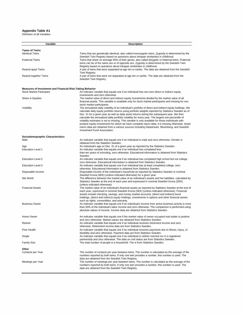
Appendix Table A1Definition of all Variables

Variable Description

Types of TwinsIdentical Twins Twins that are genetically identical, also called monozygotic twins. Zygosity is determined by the

Swedish Twin Registry based on questions about intrapair similarities in childhood.Fraternal Twins Twins that share on average 50% of their genes, also called dizygotic or fraternal twins. Fraternal

twins can be of the same sex or of opposite sex. Zygosity is determined by the Swedish Twin Registry based on questions about intrapair similarities in childhood.

Reared apart Twins A pair of twins that were separated at age ten or earlier. The data are obtained from the Swedish Twin Registry.

Reared together Twins A pair of twins that were not separated at age ten or earlier. The data are obtained from the Swedish Twin Registry.

Measures of Investment and Financial Risk-Taking BehaviorStock Market Participant An indicator variable that equals one if an individual has non-zero direct or indirect equity

investments and zero otherwise.Share in Equities The market value of direct and indirect equity investments divided by the market value of all

financial assets. This variable is available only for stock market participants and missing for non stock market participants.

Volatility The annualized daily volatility of an individual's portfolio of direct and indirect equity holdings. We calculate daily equity portfolio returns using portfolio weights reported by Statistics Sweden as of Dec. 31 for a given year as well as daily asset returns during the subsequent year. We then calculate the annualized daily portfolio volatility for every year. The largest one percentile of volatility estimates is set to missing. This variable is only available for those individuals with positive equity investments for which we have complete return data, it is missing otherwise. Asset return data are obtained from a various sources including Datastream, Bloomberg, and Swedish Investment Fund Association.

Sociodemographic CharacteristicsMale An indicator variable that equals one if an individual is male and zero otherwise. Gender is

obtained from the Statistics Sweden.Age An individual's age on Dec. 31 of a given year as reported by the Statistics Sweden.Education Level 1 An indicator variable that equals one if an individual has completed less

than ten years of schooling, zero otherwise. Educational information is obtained from Statistics Sweden.

Education Level 2 An indicator variable that equals one if an individual has completed high school but not college, zero otherwise. Educational information is obtained from Statistics Sweden.

Education Level 3 An indicator variable that equals one if an individual has at least completed college, zero otherwise. Educational information is obtained from Statistics Sweden.

Disposable Income Disposable income of the individual's household as reported by Statistics Sweden in nominal Swedish Krona (SEK) (unless indicated otherwise) for a given year.

Net Worth The difference between the market value of an individual's assets and her liabilities, calculated by Statistics Sweden at the end of each year and expressed in nominal Swedish Krona (SEK) (unless indicated otherwise).

Financial Assets The market value of an individual's financial assets as reported by Statistics Sweden at the end of each year, expressed in nominal Swedish Krona (SEK) (unless indicated otherwise). Financial assets include checking, savings, and money market accounts, (direct and indirect) bond holdings, (direct and indirect) equity holdings, investments in options and other financial assets such as rights, convertibles, and warrants.

Business Owner An indicator variable that equals one if an individual's income from active business activity is more than 50% of the individual's labor income and zero otherwise. The comparison is performed using absolute values of income. Income data are obtained from Statistics Sweden.

Home Owner An indicator variable that equals one if the market value of owner occupied real estate is positive and zero otherwise. Market values are obtained from Statistics Sweden.

Retired An indicator variable that equals one if an individual receives retirement income and zero otherwise. Retirement income data are from Statistics Sweden.

Poor Health An indicator variable that equals one if an individual receives payments due to illness, injury, or disability and zero otherwise. Payment data are from Statistics Sweden.

Single An indicator variable that equals one if an individual is neither married nor in a registered partnership and zero otherwise. The data on civil status are from Statistics Sweden.

Family Size The total number of people in a household. The is from Statistics Sweden.

OtherContacts per Year The number of contacts per year between twins. The number is calculated as the average of the

numbers reported by both twins. If only one twin provides a number, this number is used. The data are obtained from the Swedish Twin Registry.

Meetings per Year The number of meetings per year between twins. The number is calculated as the average of the numbers reported by both twins. If only one twin provides a number, this number is used. The data are obtained from the Swedish Twin Registry.

Figure 1Correlations by Genetic Similarity

0.00

0.10

0.20

0.30

0.40

0.50

0.60

0.70

0.80

Stock Market Participant Share in Equities Volatility

Identical Twins

Fraternal Twins - AllFraternal Twins - Same SexFraternal Twins - Opposite Sex

Random Sample

Figure 2:Share in Equities: Correlations by Age Group

0.00

0.10

0.20

0.30

0.40

0.50

0.60

0.70

0.80

Age < 30 30 ≤ Age < 55 55 ≤ Age < 80 Age ≥ 80

Identical Twins

Fraternal Twins

Figure 3:Share in Equities: Variance Components by Age Group

0%

10%

20%

30%

40%

50%

60%

70%

80%

90%

100%

Age < 30 30 ≤ Age < 55 55 ≤ Age < 80 Age ≥ 80

Additive Genetic Effect (A) Shared Environmental Effect (C) Individual-specific Error (E)

Figure 4:Share in Equities: Variance Components by Contact Intensity

0%

10%

20%

30%

40%

50%

60%

70%

80%

90%

100%

Little Contact Intermediate Contact Lots of Contact

Additive Genetic Effect (A) Shared Environmental Effect (C) Individual-specific Error (E)

Figure 5:Share in Equities: Correlation by Contact Intensity

0.00

0.10

0.20

0.30

0.40

0.50

0.60

0.70

0.80

Little Contact Intermediate Contact Lots of Contact

Identical Twins

Fraternal Twins