Submitted, accepted and published by Environmental Pollution 2013, 183, 166-174

Nature and Sources of Particle Associated Polycyclic Aromatic Hydrocarbons

(PAH) in the Atmospheric Environment of an Urban Area M.S. Callén

*, J.M. López, A. Iturmendi, A.M. Mastral

Department of Energy and Environment, Instituto de Carboquímica (ICB-CSIC), Zaragoza, 50018, Spain

*Corresponding author: E-mail: marisol@icb.csic.es, Tel +34 976 733977, Fax: +34 976 733318

Abstract

The total PAH associated to the airborne particulate matter (PM10) was apportioned by one

receptor model based on positive matrix factorization (PMF) in an urban environment (Zaragoza

city, Spain) during February 2010-January 2011. Four sources associated with coal combustion,

gasoline, vehicular and stationary emissions were identified, allowing a good modelling of the total

PAH (R2=0.99). A seasonal behaviour of the four factors was obtained with higher concentrations

in the cold season. The NE direction was one of the predominant directions showing the negative

impact of industrial parks, a paper factory and a highway located in that direction. Samples were

classified according to hierarchical cluster analysis obtaining that, episodes with the most negative

impact on human health (the highest lifetime cancer risk concentrations), were produced by a higher

contribution of stationary and vehicular emissions in winter season favoured by high relative

humidity, low temperature and low wind speed.

Keywords: PM10; PAH; receptor model; PMF; source apportionment.

Episodes with the most negative impact on human health regarding PAH were produced by a higher

contribution of stationary and vehicular emissions in winter season.

1. INTRODUCTION

The study of the air quality in cities is quite interesting from an environmental point of view,

especially due to the negative potential impact that anthropogenic activities can have on human

health. Polycyclic aromatic hydrocarbons (PAH) are a group of organic compounds containing only

carbon and hydrogen and constituted by two or more aromatic rings fused together. They have been

regarded as persistent organic pollutants (POPs) and they are mainly formed by incomplete

combustion processes of organic materials such as biomass combustion, vehicular emissions,

industrial processes, etc (Katsoyiannis et al., 2011; Manoli et al., 2004; Ravindra et al., 2008;

Simoneit, 2002). Their main concern is related to their potential exposure and adverse health effects

on humans (Boström et al. 2002; Gammon and Santella, 2008; Luch et al., 2005; Okona-Mensah et

al., 2005; Rybicki et al., 2006) so that some of them have been identified as carcinogenic,

mutagenic and teratogenic. The US-EPA (2001) has classified seven PAH (benzo[a]pyrene (BaP),

benz[a]anthracene, chrysene, benzo[b]fluoranthene, benzo[k]fluoranthene, dibenz[a,h]anthracene,

and indeno[1,2,3-cd]pyrene) as Group B2, probable human carcinogens. These seven PAH have

also been classified by the International Agency for Research on Cancer (IARC, 2010) where

benz[a]anthracene and BaP are considered as Group 2A, probable human carcinogens and the other

PAH as possible human carcinogens (Group 2B). The UK air quality standard for BaP is 0.25 ng/m3

according to the Expert Panel on Air Quality (EPAQS, 1999). This concentration was adopted as a

provisional national air quality strategy objective for England, Wales and Scotland to be achieved

by 31 December 2010. In Europe, the Directive 2004/107/EC establishes a target value of BaP= 1.0

ng/m3 for the total content in the PM10 fraction averaged over a calendar year to be achieved by 31

December 2012. Although the knowledge of the pollutant concentrations constitutes one of the first

steps in the air quality, the scope for making further reductions in polluting emissions is aimed to

avoid the risk to human health protecting the environment as a whole. This is the reason why it is

important to discern the main pollution sources affecting air quality. In this way, receptor models

have been widely used (Bzdusek et al., 2004; Kim et al., 2003; Park et al., 2011; Xie et al., 2010;

Zhang et al., 2012) as tools that assess contributions from various sources based on observations at

sampling sites.

In this work, the total PAH concentrations bound to the PM10 were modelled by a PMF model by

first time in a Spanish city. The conditional probability function and cluster analysis allowed

distinguishing the main directions contributing to total PAH for each identified source and

classifying PAH samples, which were interpreted as a function of the meteorological conditions and

the risk for human health. The aim was to provide a better knowledge on the PAH pollution sources

in order to improve air quality policies, which could further reduce harmful effects on human

health.

2. MATERIALS AND METHODS

2.1 Sampling description

The study was performed in Rio Ebro Campus (length= 41.68, latitude= -0.89), University of

Zaragoza. It belongs to Rey Fernando quarter, a residential area located at the North of Zaragoza

city (Spain) (Figure 1). The sampling location was a sub-urban area mainly influenced by vehicle

traffic due to the proximity of the AP-2 highway (~50 m) joining Zaragoza with Barcelona (daily

average intensity in 2011 =11 420 vehicles, 11.2% of heavy-duty vehicles), heating oil and natural

gas combustion for domestic heating, agricultural burning, wood combustion (small villages) and

industrial emissions (industrial parks located in the surroundings of the city, paper fabrics and

power stations). The sampling site has been previously described in detail (Callén et al., 2008a,

2009) although during this campaign, it is worthy pointing out that the site was influenced by

construction activities carried out in order to increase the number of lines in the AP-2 highway.

2.2. Sampling campaign

A Graseby Andersen high-volume air sampler (1.13 m3/min), provided with a PM10 cut off inlet at

10 m and located 3.5 m from the ground, was used to collect particulate phase PAH over quartz

fibre filters QF1-150 (20x25 cm) provided by MCV, S.A. Seven samples per month (each sample

corresponding to one day of a continuous week, time of sampling=24 hours) were collected from

February 1st, 2010 to January 16th, 2011, obtaining a total of 84 samples. Briefly, filters were

cleaned-up by Soxhlet with dichloromethane (DCM) previous to the sampling. PM10 mass

concentration was determined gravimetrically by weighting the filters, before and after sampling in

a microbalance (accuracy 10 g), once the filters were conditioned in desiccators. More details

regarding the sampling method were given in previous articles (Callén et al., 2008a; López et al.,

2005).

2.3 PAH analysis

The following PAH (phenanthrene (Phe), anthracene (An), 2+2/4-methylphenanthrene

(2+2/4MePhe), 9-methylphenanthrene (9MePhe), 1-methylphenanthrene (1MePhe), 2,5-/2,7-/4,5-

dimethylphenanthrene (DiMePhe), fluoranthene (Flt), pyrene (Py), benzaanthracene (BaA),

chrysene (Chry), benzobfluoranthene (BbF), benzojfluoranthene (BjF), benzokfluoranthene

(BkF), benzoepyrene (BeP), benzoapyrene (BaP), indeno1,2,3-cdpyrene (IcdP),

dibenza,hanthracene (DahA), benzoghiperylene (BghiP) and coronene (Cor) were quantified

according to previous publications using gas chromatography mass spectrometry mass spectrometry

(GC-MS-MS) (Table 1S, Supplementary Information)(Callén et al., 2008b). Briefly, ¼ of the filter

was extracted by Soxhlet with dichloromethane after the addition of a surrogate standard solution

(An-d10+BaP-d12+BghiP-d12). After concentration by rotary evaporator, samples were cleaned-up

through a silica gel column with dichloromethane and concentrated in a pure N2 stream. The solvent

was exchanged to n-hexane and p-terphenyl native was added as recovery standard. Each compound

was quantified by GC-MS-MS operating at electron impact energy of 70 eV and using the multiple

reaction monitoring (MRM) mode. A Varian Select PAH capillary column (30 m x 0.25 mm

internal diameter x 0.25 m film thickness) was used to quantify PAH and 1 L of sample was

injected in splitless mode. The GC conditions were: 1.5 ml/min Helium flow; temperature-time

programme: 70ºC, 1 min, increasing 10º/min till 325ºC and isotherm for 18.5 minutes. The injector

temperature was set to 280ºC, the transfer line to 300ºC, the ion trap to 220ºC and the manifold to

60ºC. The identification and quantification of PAH was done according to retention times and the

internal standard method relative to the closest eluting PAH surrogate. Calibration curves were

prepared with PAH concentrations between 20-1000 ppb in n-hexane. The concentrations of the

surrogate and recovery standard were the same and identical as those of the sample extracts. The

correlation coefficients of the calibration curve for the different PAH were R2>0.99.

2.4. Quality assurance

Repeatability was evaluated by performing four analyses of a standard PAH solution containing the

above mentioned PAH and the surrogate and the recovery standards (250 ppb) the same day in the

same conditions. Reproducibility was also evaluated by performing analysis of that standard on six

different days. In both cases, relative standard deviations (RSD) of the relative response factors

were below the 10% for all PAH. The accuracy of the method was determined by analysing the

Standard Reference Material (SRM1649a, Urban Dust) from the National Institute of Standards and

Technology (NIST) (40 mg, n=4) obtaining errors below the 25% (with the exception of An, 28%).

Both field and laboratory blank samples were prepared and analyzed and all data were corrected

with reference to a blank. The method detection (DL) and quantification limits (QL) were

calculated as the concentrations equivalent to three and ten times the noise of the quantifier ion for a

blank sample (sample air volume=1600 m3) (QL ranged from 0.01 ng/m

3 (DiMePhe) to 0.08 ng/m

3

(Phe). Recovery efficiencies of surrogate deuterated PAH between 75-108% were achieved and no

corrections were applied to PAH samples.

2.5 PMF model

The EPA positive matrix factorization (PMF) model (3.0 software program) was applied to all

samples in order to apportion the main PAH pollution sources. Rather than considering the

theoretical approach of this model, which has already been described in detail in different

publications (Chueinta et al., 2000; Paatero and Tapper, 1994; Paatero, 1997), this paper was

focused on the model considerations. As with other receptor models based on statistical factor

analysis, numerous procedural decisions have to be made when running this model because results

may be sensitive to these decisions. In particular, analysis is limited by the accuracy, precision and

range of species measured at the receptor site. However, one of the main advantages of the PMF

model with regard to other receptor models is the use of the uncertainty matrix so that

concentrations below the detection limit can be underweighted. Concentrations below the detection

limit were substituted by half the detection limit and their overall uncertainties were set at five-

sixths of the detection limit values (Polissar et al., 1998). There were no missing data. Sample

specific uncertainties were provided according to Sij= DL/3+c*xij, where sij= uncertainty, DL

=detection limit, c =constant (0.1 if xij>3*DL, 0.2 if Xij<3*DL) and xij=variable (Chueinta et al.,

2000).

A critical step in PMF analysis is determining the correct number of factors. The optimal number of

factors (p) was achieved based on: the closeness of QRobust to QTheoretical (QTheoreticaln*m-p*(n+m)

where n= number of samples, m= number of variables and p= number of factors); the maximum

individual column mean of the scaled residual matrix (IM); the maximum individual column

standard deviation of the scaled residual matrix (IS); the majority of scaled residuals between -3 and

3; the absence or a reduced number of non-explained species (non-explained variation: NEV <

0.25) and the physical significance of the solution found (Chueinta et al., 2000; Juntto and Paatero,

1994; Lee et al., 1999; US-EPA, 2008).

The data set used was an 84x17 matrix (sample number, number of compounds) and the model was

run in the default robust mode to decrease the influence of extreme values on the PMF solution. Only

one variable, the total PAH was down-weighted as a weak variable and the data were fitted using 17

strong variables (Phe, An, 2+2/4MePhe, 9MePhe, 1MePhe, Flt, Py, BaA, Chry, BbF, BkF, BjF,

BeP, BaP, IcdP+DahaA, BghiP, Cor). Solutions between three and seven factors were considered

and the optimal solution extracted four factors by running the data with 20 initial random starting

points and 10% extra modelling uncertainty. The Q theoretical was 1024, the Q robust 1243.9 and

the Q true 1249.1. To ensure that the appropriate number of factors was chosen, the scaled residuals

were also examined. A reasonable solution should have scaled residuals distributed mostly between

-3 and +3, obtaining 88% of the scaled residuals estimated by PMF distributed in that way. Fpeak

model was run with strength of fpeak of 0.1 although no variations were found. A bootstrap model

run was also carried out by running 100 bootstraps with a minimum correlation value of 0.6. The

percentage of bootstrapped factors assigned (mapped) to their corresponding base factors is

indicative of the uniqueness of a given factor profile. When a high amount of a given bootstrapped

factor is spread over more than one base factor, it may suggest that the factor profile solutions are

not unique and the number of factors may have to be reduced (Sofowote et al., 2011) (Table 2S,

Supplementary Information).

2.6. Conditional probability function

The conditional probability function (CPF), which is the conditional probability that a given factor

contribution from a given wind direction will exceed a predetermined threshold criterion, was used.

Local meteorological data (wind speed and direction) and source contributions from the PMF

analysis were combined to identify the likely directions of the PAH sources.

The formula of the CPF is:

where mΔθ is the number of occurrences from wind sector Δθ where the source contributions are in

the upper 25th

percentile, and nΔθ is the total number of occurrence from this wind sector. A total of

12 sectors were considered in this study (Δθ = 30°).

2.7 Statistical tools

Statistical analysis, including ANOVA and t-test were performed using Software SPSS 16.0. A one-

way ANOVA procedure was performed to test the significant differences of the dataset and PMF

contribution factors. SPSS was also used to classify samples according to hierarchical cluster

analysis using Ward method to data from the contributions of the PMF model.

2.8 BaP-eq and lifetime lung cancer risk

The BaP equivalent concentration (BaP-eq), which considers not only the carcinogenic character of

BaP but also other PAH, was calculated by summing the products of each PAH concentration and

their respective toxic equivalent factor (TEF). In this case, the TEF calculated by Larsen and Larsen

(1998) were used.

The lifetime lung cancer risk was calculated with the formula:

Lifetime lung cancer risk = BaP-eq (ng/m3) × UR

where UR is the inhalation unit risk of exposure to BaP (the calculated, theoretical upper limit

possibility of contracting cancer when exposed to BaP at a concentration of one nanogram per cubic

meter of air for a 70 year lifetime) (OEHHA 1993, 2005). In this work, the UR= 8.7 × 10–5

per

ng/m3 was taken according to the World Health Organization (WHO), based on an epidemiology

study on coke-oven workers in Pennsylvania (WHO 2000).

3. RESULTS AND DISCUSSION

3. 1. PM10 temporal variations

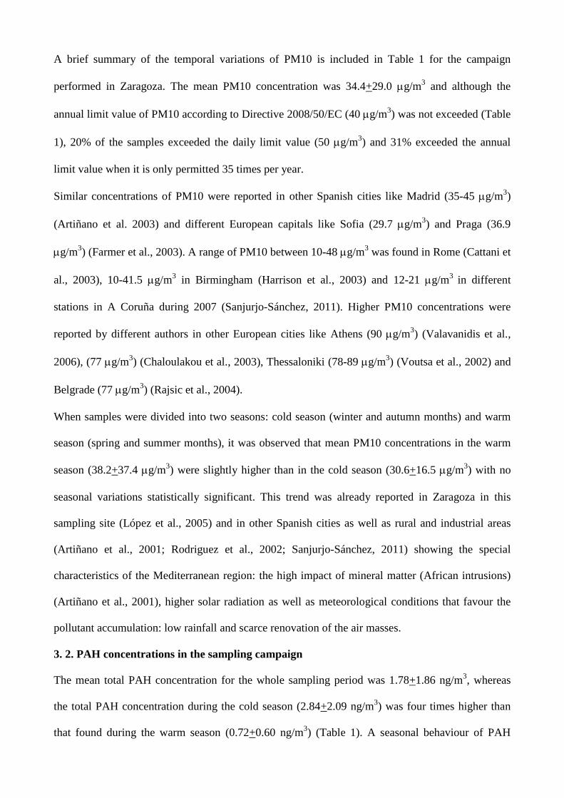
A brief summary of the temporal variations of PM10 is included in Table 1 for the campaign

performed in Zaragoza. The mean PM10 concentration was 34.4+29.0 g/m3 and although the

annual limit value of PM10 according to Directive 2008/50/EC (40 g/m3) was not exceeded (Table

1), 20% of the samples exceeded the daily limit value (50 g/m3) and 31% exceeded the annual

limit value when it is only permitted 35 times per year.

Similar concentrations of PM10 were reported in other Spanish cities like Madrid (35-45 g/m3)

(Artiñano et al. 2003) and different European capitals like Sofia (29.7 g/m3) and Praga (36.9

g/m3) (Farmer et al., 2003). A range of PM10 between 10-48 g/m

3 was found in Rome (Cattani et

al., 2003), 10-41.5 g/m3 in Birmingham (Harrison et al., 2003) and 12-21 g/m

3 in different

stations in A Coruña during 2007 (Sanjurjo-Sánchez, 2011). Higher PM10 concentrations were

reported by different authors in other European cities like Athens (90 g/m3) (Valavanidis et al.,

2006), (77 g/m3) (Chaloulakou et al., 2003), Thessaloniki (78-89 g/m

3) (Voutsa et al., 2002) and

Belgrade (77 g/m3) (Rajsic et al., 2004).

When samples were divided into two seasons: cold season (winter and autumn months) and warm

season (spring and summer months), it was observed that mean PM10 concentrations in the warm

season (38.2+37.4 g/m3) were slightly higher than in the cold season (30.6+16.5 g/m

3) with no

seasonal variations statistically significant. This trend was already reported in Zaragoza in this

sampling site (López et al., 2005) and in other Spanish cities as well as rural and industrial areas

(Artiñano et al., 2001; Rodriguez et al., 2002; Sanjurjo-Sánchez, 2011) showing the special

characteristics of the Mediterranean region: the high impact of mineral matter (African intrusions)

(Artiñano et al., 2001), higher solar radiation as well as meteorological conditions that favour the

pollutant accumulation: low rainfall and scarce renovation of the air masses.

3. 2. PAH concentrations in the sampling campaign

The mean total PAH concentration for the whole sampling period was 1.78+1.86 ng/m3, whereas

the total PAH concentration during the cold season (2.84+2.09 ng/m3) was four times higher than

that found during the warm season (0.72+0.60 ng/m3) (Table 1). A seasonal behaviour of PAH

statistically significant at 99% level was found with higher concentrations in the cold period and

lower concentrations during the warm season. This seasonal behaviour has already been reported by

different authors (Chen et al., 2009; Holoubek et al., 2007; Lammel et al., 2010) due to the

influence of the meteorological conditions: low temperature, low solar radiation, low photochemical

degradation and increased emissions by anthropogenic sources, like domestic heating, in the cold

period.

The dominant PAH were Phe, BaA, Chry, Flt, Py, BbF and BghiP with a percentage value of 65%

(46-79%). These PAH are associated with fossil fuel, coal and biomass combustion sources

including vehicular emissions (Ravindra et al., 2008) although the origin of the possible pollution

sources will be faced in more detail in the next section. One of the most interesting PAH to study

due to its carcinogenic and mutagenic character is the BaP. The mean BaP concentration was

0.09+0.11 ng/m3 and although the guideline value of BaP =1.0 ng/m

3 according to Directive

2004/107/EC was not exceeded during this campaign, the UK Air Quality guideline value of 0.25

ng/m3 was exceeded in 11% of the samples, all of them in winter season. BaP is considered one of

the most carcinogenic PAH, nevertheless this PAH can underestimate the carcinogenic character of

the particulate matter (Wickramasinghe et al., 2012). This is the reason why the BaP-eq was

calculated for each individual sample by taking into account the TEF (Larsen and Larsen, 1998) of

different PAH. As happened with the BaP, the mean BaP-eq concentrations were higher during the

cold season (0.29+0.23 ng/m3), involving a higher potential risk for human health.

3.3. PAH source apportionment by PMF

A total of four factors associated to the particle total PAH were apportioned by the PMF model. The

model performance was quite good with an R2= 0.99, slope=1 (Figure 1S, Supplementary

information) and the standard error of the estimates for each individual PAH was less than 20%

(exception An=26%) (Table 3S, Supplementary information).

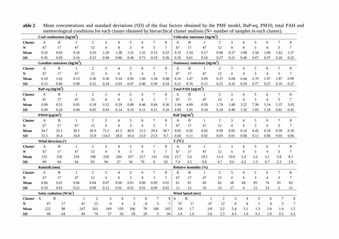
Figure 2 shows the contribution of each factor and the source profiles for the PMF resolved factors.

The first factor mainly characterized by 2+2/4 MePhe, Phe, Flt and Py contributed 24% to the total

PAH. The presence of Flt, Phe and An can be attributed to both coal combustion and vehicular

exhaust emissions (Abrantes et al., 2004; Ho et al., 2002). Coal is one of the main fuels used in

Aragón for power generation representing 25% of the generated energy in 2008 so this factor was

considered as coal combustion emissions. As shown in the time series plot (Figure 3), the highest

source contributions were on the 13/12/2010 and the 01/02/2010 but also the 09/06/2010 indicating

that although the contribution of the heating systems in the winter season could be reflected,

industrial parks using this fuel and coal power stations located in Teruel province were mainly

responsible of this factor along the year. The conditional probability function (Figure 3) indicated

the higher contribution of this factor during the cold period in the NE direction whereas during the

warm seasons, the transport from the S and SE directions, where several coal power stations are

installed, influenced on the PAH concentrations.

The second factor exhibited the highest source contribution, 32% of the total PAH and it was

mainly associated with BkF, BbF, BjF, IcdP+DahA and BghiP. The factor accounted for 83% and

61% of the total BkF and IcdP+DahA, respectively. BbF and BkF are typical markers of diesel

emissions (Harrison et al., 1996; Lee et al., 2004). IcdP was associated with diesel and also gasoline

emissions (Boström et al., 2002; Ravindra et al., 2008; Riddle et al., 2007). Diesel exhaust is known

to contain more particulate matter than gasoline exhaust, and heavier PAH, such as DahA, BghiP

and IcdP are associated with these particles (Cristale et al., 2012; Manoli et al., 2004; Ravindra et

al., 2008; Umbuzeiro et al., 2008). Different authors also attributed the high contribution of high

molecular weight to both maritime and airport traffic emissions (Contini et al., 2011; Lee et al.,

2004; Moldanová et al., 2009). The CPF (Figure 3) plot for this factor points that high source

contribution was more likely related to an easterly wind direction in the cold period suggesting an

impact from the highways and an industrial park known as “Ciudad del Transporte” (Figure 1)

where most of the heavy-duty vehicles are parked. This industrial park is located at 6 km from the

North of Zaragoza, close to the A-23 and A-2 highways and it is composed by more than 20

factories related with the transport and logistics. During the warm seasons, it pointed to the S-W

showing the influence of the airport and the central train/bus station so this factor was considered as

vehicular emissions.

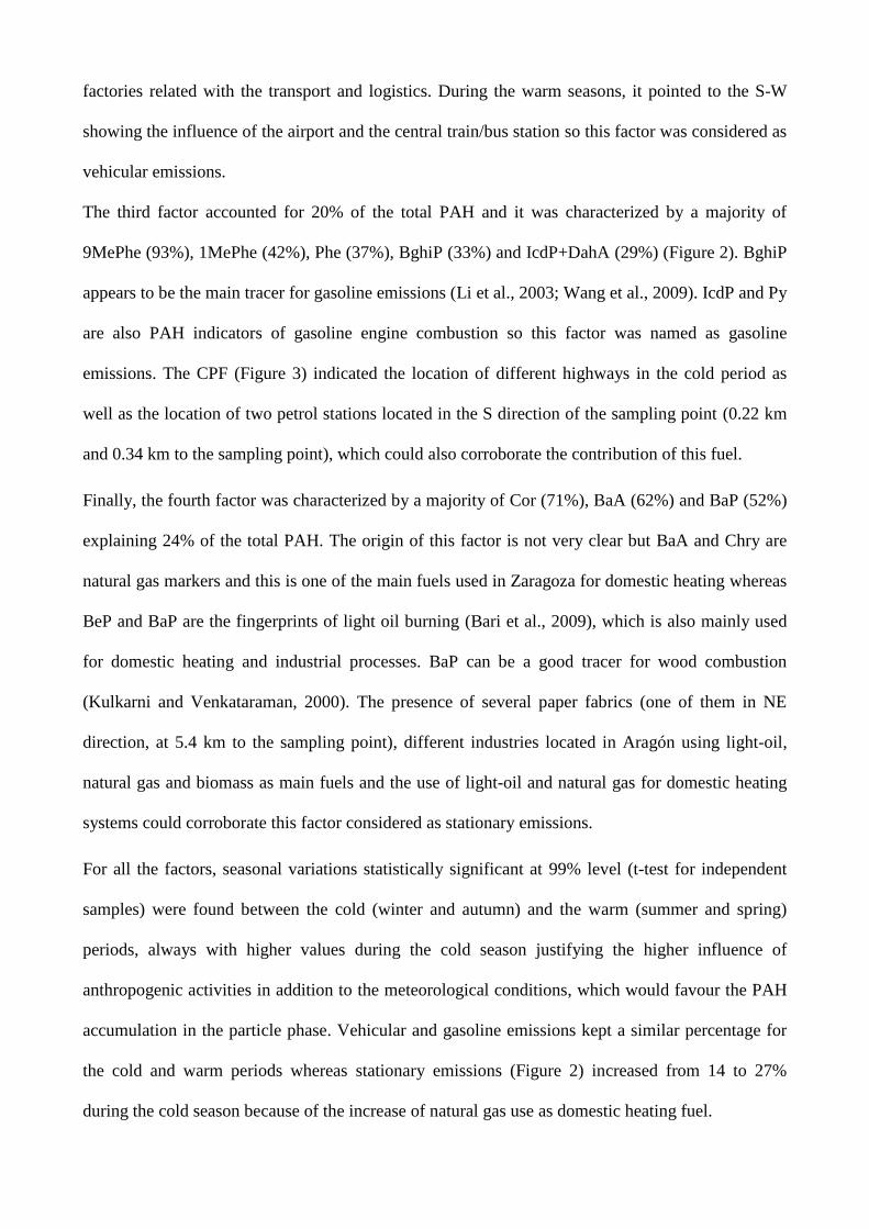
The third factor accounted for 20% of the total PAH and it was characterized by a majority of

9MePhe (93%), 1MePhe (42%), Phe (37%), BghiP (33%) and IcdP+DahA (29%) (Figure 2). BghiP

appears to be the main tracer for gasoline emissions (Li et al., 2003; Wang et al., 2009). IcdP and Py

are also PAH indicators of gasoline engine combustion so this factor was named as gasoline

emissions. The CPF (Figure 3) indicated the location of different highways in the cold period as

well as the location of two petrol stations located in the S direction of the sampling point (0.22 km

and 0.34 km to the sampling point), which could also corroborate the contribution of this fuel.

Finally, the fourth factor was characterized by a majority of Cor (71%), BaA (62%) and BaP (52%)

explaining 24% of the total PAH. The origin of this factor is not very clear but BaA and Chry are

natural gas markers and this is one of the main fuels used in Zaragoza for domestic heating whereas

BeP and BaP are the fingerprints of light oil burning (Bari et al., 2009), which is also mainly used

for domestic heating and industrial processes. BaP can be a good tracer for wood combustion

(Kulkarni and Venkataraman, 2000). The presence of several paper fabrics (one of them in NE

direction, at 5.4 km to the sampling point), different industries located in Aragón using light-oil,

natural gas and biomass as main fuels and the use of light-oil and natural gas for domestic heating

systems could corroborate this factor considered as stationary emissions.

For all the factors, seasonal variations statistically significant at 99% level (t-test for independent

samples) were found between the cold (winter and autumn) and the warm (summer and spring)

periods, always with higher values during the cold season justifying the higher influence of

anthropogenic activities in addition to the meteorological conditions, which would favour the PAH

accumulation in the particle phase. Vehicular and gasoline emissions kept a similar percentage for

the cold and warm periods whereas stationary emissions (Figure 2) increased from 14 to 27%

during the cold season because of the increase of natural gas use as domestic heating fuel.

3.4. Cluster analysis and lifetime lung cancer risk

Hierarchical cluster analysis was applied to the contribution of the different factors obtained by the

PMF model obtaining a dendogram with the Ward method (Figure 2S, Supplementary Information)

and the Euclidean distance square that allowed classifying samples by cases. The results obtained

by the dendogram were studied and interpreted by taking into account not only the PMF factors but

also the meteorological conditions, the PM10 and the BaP-eq concentrations. In fact, one of the

main concerns of PAH study is related to the carcinogenic character of PAH.

A total of eight different clusters were obtained (Table 2) although these could be classified into

two major clusters: A (cluster 1+2+3+4) and B (Cluster 5+6+7+8) (Figure 4) corresponding to 80%

and 20% of the samples. Trying to discern the main difference between both clusters, an

independent t-test was carried out and the variables statistically significant at 95% between these

two major clusters were: the vehicular, the gasoline and the stationary emissions, the BaP, BaP-eq,

the total PAH and most of the meteorological variables: T, wind direction, relative humidity, solar

radiation and wind speed. The characteristics of the meteorological conditions for the first cluster A,

associated with low total PAH concentrations and lower contributions of PMF factors, were high

temperature (Table 2) (15.7ºC versus 5.6ºC), high solar radiation (222 W/m2 versus 98 W/m

2) and

lower relative humidity (61% versus 81%) with higher wind speed (3.8 m/s versus 1.7 m/s), typical

conditions of the warm period favouring the pollutant dispersion and possible photo-degradation. In

fact, 63% of the samples corresponded to the warm season whereas only 15% of the samples took

place in winter season. On the contrary, the second main cluster B (20% of the samples), with

higher total PAH concentrations and higher contributions of the PMF factors, showed typical

meteorological conditions of the cold period; 76% of the samples corresponded to winter season

and 24% to autumn season. The first main cluster: A (80% of the samples), associated with most of

the samples, could be divided into two main subgroups representing 71% (cluster 1+cluster 2=60

samples) and 8% (cluster 3+cluster 4= 7 samples) of the total samples. The variables statistically

significant at 95% between both subgroups were the coal combustion, the BaP, the BaP-eq, the total

PAH and the temperature and solar radiation. Again the cluster with lower number of samples (8%)

showed the highest concentrations of coal combustion, BaP, BaP-eq and total PAH with lower

temperature (8ºC versus 17ºC) and solar radiation (169 versus 227 W/m2).

The second main cluster: B representing 20% of the total of the samples was also studied by an

independent t-test. This cluster was characterized by cluster 5 (3.7%) and cluster 6+7+8 (17%). In

this case, although no variations statistically significant at 95% level were found for the

meteorological conditions, it was observed that the vehicular and the stationary emissions showed

significant variations with higher contributions of these factors for the lower number of samples

(3.7%) reflecting the impact of these anthropogenic pollution sources.

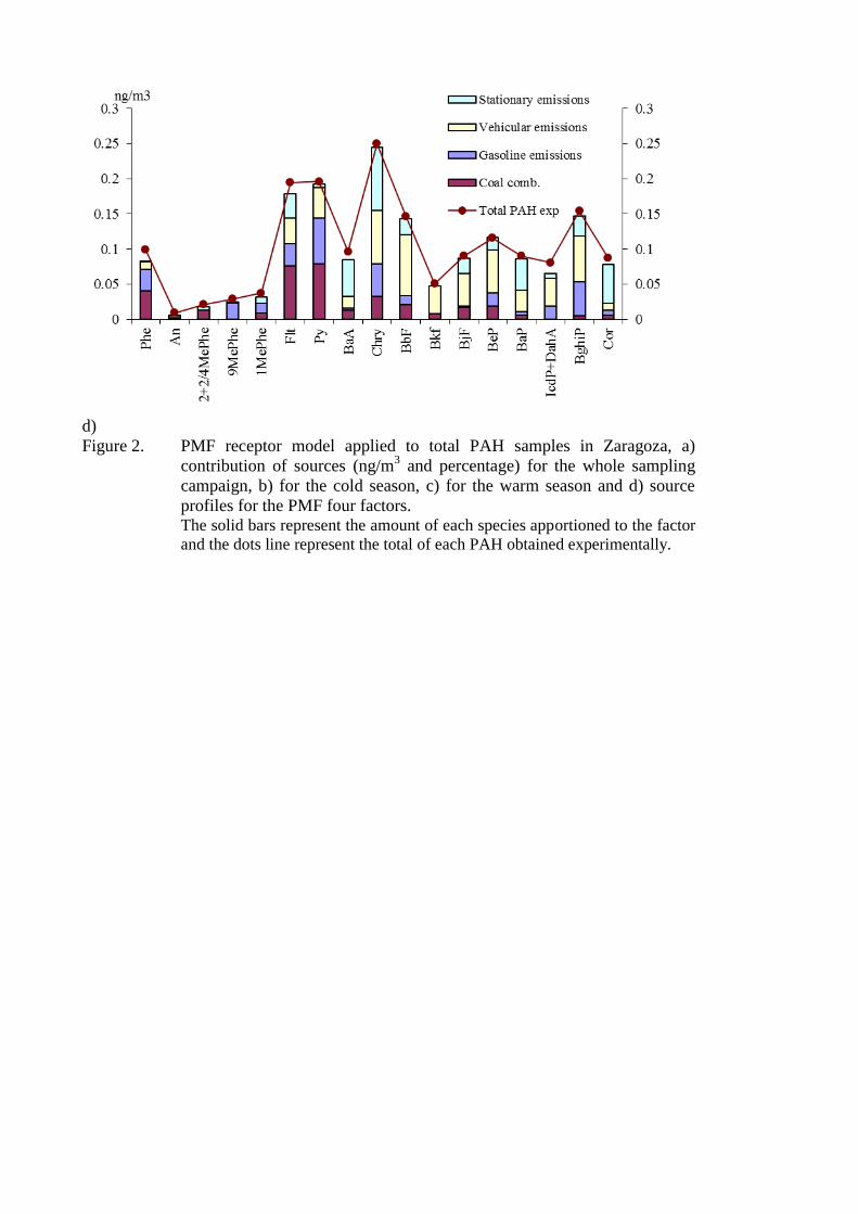
The contribution of each PMF factor for each one of the eight clusters obtained by the dendogram

was represented in Figure 4. It was also plotted the estimated lifetime lung cancer risk from PAH in

the atmosphere. Regarding the factors contributing to this carcinogenic character, it was observed

that stationary emissions followed by vehicular emissions contributed majority to the total PAH.

Cluster 5 showed the highest lifetime lung cancer risks with an average value of 7.0 x 10-5

(7

additional cases per 100 000 people exposed), which was higher than the target excess individual

lifetime risk, which is 10-6

(US-EPA, 2012). All these episodes were produced in winter season

(02/02/2010, 03/02/2010, 14/01/2011) and were characterized by low temperature (3ºC), high

relative humidity (85%), low solar radiation (13 W/m2) and low wind speed (1.3 m/s). For the

03/02/2010 there was some rain and for the 14/01/2011, there was foggy weather, scenarios that

could favour the pollutant accumulation and the deposition of pollutants to the particulate matter,

respectively. The important role of climate has also been remarked by different authors (Cachada et

al., 2012; Desaules et al., 2008), indicating that the lower temperatures and the higher levels of

precipitation may enhance wet deposition process and condensation.

These results indicate that the total lifetime cancer risk of PAH in Zaragoza may represent some

concern, especially vehicular and stationary emissions, in particular during the cold season favoured

by stagnant meteorological conditions. This impact could be even more negative over the most

sensitive population: elderly people and children.

4. CONCLUSIONS

The PMF receptor model successfully allowed the identification and quantification of four sources

with similar contribution: coal combustion, vehicular emissions, gasoline emissions and stationary

emissions, associated to the total PAH bound to PM10 of Zaragoza.

The CPF showed that the NE direction was one of the prevailing directions providing high total

PAH concentrations, especially during the cold season, due to the influence of anthropogenic

activities related with industrial parks, highways and a paper fabric located in that direction.

Hierarchical cluster analysis showed that samples were classified into two major clusters whose

main differences were related to meteorological conditions and factor contributions. Episodes

involving higher risk for human health according to the lifetime cancer risk were favoured by

typical meteorological conditions of the winter season and higher contributions of the stationary and

vehicular emission factors. This corroborated the impact, not only of the anthropogenic pollution

sources but also the meteorological conditions, specially those winter days with very low

temperature, fog, no wind and high relative humidity that can be more dangerous for human health.

Acknowledgements

Authors would like to thank Aula Dei-CSIC (R. Gracia) for providing the meteorological data as

well as the Ministry of Science and Innovation (Spain) (MICIIN) and the E plan for the co-funding

through the project CGL2009-14113-C02-01. JM López (Ramón y Cajal contract) and A. Iturmendi

(contract) would also like to thank the MICYT and the MICIIN.

Appendix A. Supplementary data

Supplementary data associated with this article can be found, in the online version, at:

References

Abrantes, R., Assuncao, J., Pesquero, C.R., 2004. Emission of polycyclic aromatic hydrocarbons from

light-duty diesel vehicles exhausts. Atmospheric Environment 38, 1631-1640.

Artiñano, B., Querol, X., Salvador, P., Rodriguez, S., Alonso, D.G., Alastuey, A., 2001. Assessment of

airborne particulate levels in Spain in relation to the new EU directive. Atmospheric Environment 35,

S43 S53.

Artiñano, B., Salvator, P., Alonso, D.G., Querol, X., Alastuey, A., 2003. Anthropogenic and natural

influence on the PM(10) and PM(2.5) aerosol in Madrid (Spain). Analysis of high concentration

episodes. Environmental Pollution 125, 453–465.

Bari, M. A., Baumbach, G., Kuch, B., Scheffknecht, G., 2009. Wood smoke as a source of particle-

phase organic compounds in residential areas. Atmospheric Environment 43, 4722–4732.

Bzdusek, P.A., Christensen, E.R., Li, A., Zou, Q., 2004. Source apportionment of sediment PAHs in

Lake Calumet, Chicago: application of factor analysis with nonnegative constraints. Environmental

Science and Technology 38, 97–103.

Boström, C.E., Gerde, P., Hanberg, A., Jernström, B., Johansson, C., Kyrklund, T., Rannug, A.,

Törnqvist, M., Victorin, K., Westerholm, R., 2002. Cancer risk assessment, indicators and

guidelines for polycyclic aromatic hydrocarbons in the ambient air. Environmental Health

Perspectives 110, 451-488.

Cachada, A., Pato, P., Rocha-Santos, T., Ferreira da Silva, E., Duarte, A.C., 2012. Levels, sources

and potential human health risks of organic pollutants in urban soils. The Science of the total

Environment 430, 184-192.

California Environmental Protection Agency (CalEPA). 1997. Air Toxics Hot Spots Program Risk

Assessment Guidelines: Technical Support Document for Determining Cancer Potency Factors.

Draft for Public Comment. Office of Environmental Health Hazard Assessment, Berkeley, CA.

Callén, M.S., de la Cruz, M.T., López, J.M., Murillo, R., Navarro, M.V. and Mastral, A.M., 2008a.

Long-range atmospheric transport and local pollution sources on PAH concentrations in a South-

European urban area. Fulfilling of the European Directive. Water Air and Soil Pollution 190, 271-

285.

Callén, M.S., de la Cruz, M.T., López, J.M., Murillo, R., Navarro, M.V. and Mastral, A.M., 2008b.

Some inferences on the mechanism of atmospheric gas-particle partitioning of PAH at Zaragoza

(Spain). Chemosphere 73, 1357-1365.

Callén, M.S., de la Cruz, M.T., López, J.M., Navarro, M.V., and Mastral, A.M., 2009. Comparison

of receptor models for source apportionment of the PM10 in Zaragoza (Spain). Chemosphere 76,

1120-1129.

Cattani, G., Cusano, M.C., Inglessis, M., Settimo, G., Stacchini, G., Ziemacki, G., Marconi, A.,

2003. Particulate matter measurement of PM2.5 and PM10 in Rome: comparison indoor/outdoor.

Annals, Instituto Superiore di Sanita 39, 357–364.

Chaloulakou, A., Kassomenos, P., Spyrellis, N., Demokritou, P., Koutrakis, P., 2003.

Measurements of PM10 and PM2.5 particle concentrations in Athens, Greece. Atmospheric

Environment 37, 649–660.

Chen, K.S., Li, H.C., Wang, H.K., Wang, W.C, Lai, C.H., 2009. Measurement and receptor

modeling of atmospheric polycyclic aromatic hydrocarbons in urban Kaohsiung, Taiwan. Journal of

Hazardous Materials 166, 873–879.

Chueinta, W., Hopke, P.K., Paatero, P., 2000. Investigation of sources of atmospheric aerosol at

urban and suburban residential areas in Thailand by positive matrix factorization. Atmospheric

Environment 34, 3319–3329.

Contini, D., Gambaro, A., Belosi, F., De Pieri, S., Cairns, W.R.L., Donateo, A., Zanotto, E., Citron,

M., 2011. The direct influence of ship traffic on atmospheric PM2.5, PM10 and PAH in Venice.

Journal of Environmental Management 92, 2119–2129.

Cristale, J., Silva, F.S., Zocolo, G.J., Marchi, M.R., 2012. Influence of sugarcane burning on

indoor/outdoor PAH air pollution in Brazil. Environmental Pollution 169, 210-216.

Desaules, A., Ammann, S., Blum, F., Brandli, R.C., Bucheli, T.D., Keller, A., 2008. PAH and PCB

in soils of Switzerland-status and critical review. Journal of Environmental Monitoring 10, 1265–

1277.

Directive 2008/50/EC of the European Parliament and of the Council of 21 May 2008 on ambient

air quality and cleaner air for Europe.

Directive 1999/30/EC of 22 April 1999 relating to limit values for sulphur dioxide, nitrogen dioxide

and oxides of nitrogen, particulate matter and lead in ambient air.

Directive 2004/107/EC of the European Parliament and of the Council of 15 December 2004

relating to arsenic, cadmium, mercury, nickel and polycyclic aromatic hydrocarbons in ambient air.

EPAQS, Expert Panel on Air Quality Standards Polycyclic Aromatic hydrocarbons, 1999,

published by The Stationery Office.

Farmer, P.B., Singh, R., Kaur, B., Sram, R.J., Binkova, B., Popov, T.A., Garte, S., Taioli, E.,

Gabelova, A., Cebulska-Wasilewska, A., 2003. Molecular epidemiology studies of carcinogenic

environmental pollutants: Effects of polycyclic aromatic hydrocarbons (PAHs) en environmental

pollution on exogenous and oxidative DNA damage. Mutation Research-reviews in Mutation

Research 544(2), 397-402.

Gammon, M.D., Santella, R.M., 2008. PAH, genetic susceptibility and breast cancer risk: an update

from the long Island breast cancer study project. European Journal of Cancer 44, 636-640.

Harrison, R.M., Smith, D.J.T. and Luhana, L., 1996. Source Apportionment of Atmospheric

Polycyclic Aromatic Hydrocarbons Collected from an Urban Location in Birmingham, U.K.

Environmental Science and Technology 30(3), 825-832.

Harrison, R.M., Tilling, R., Callen-Romero, M.S., Harrad, S., Jarvis, K., 2003. A study of trace

metals and polycyclic aromatic hydrocarbons in the roadside environment. Atmospheric

Environment 37, 2391–2402.

Ho, K.F., Lee, S.C., Chiu, G.M. 2002. Characterization of selected volatile organic compounds,

PAH and carbonyl compounds at a roadside monitoring station. Atmospheric Environment 36, 57-

65.

Holoubek, I., Klánová, J., Jarkovský, J., Kohoutek, J., 2007. Trends in background levels of

persistent organic pollutants at Ko_setice observatory, Czech Republic. Part I. Ambient air and wet

deposition 1988-2005. Journal of Environmental Monitoring 9, 557-563.

IARC, 2010. Monographs on the evaluation of carcinogenic risks to humans. Some Non-

heterocyclic Polycyclic Aromatic Hydrocarbons and Some Related Exposures 92.

Juntto, S., Paatero, P., 1994. Analysis of daily precipitation data by positive matrix factorization.

Environmetrics 5, 127-144.

Katsoyiannis, A., Sweetman, A.J., Jones, K.C., 2011. PAH molecular diagnostic ratios applied to

atmospheric sources: a critical evaluation using two decades of source inventory and air

concentration data from the UK. Environmental Science and Technology 45 (20), 8897-8906.

Kim E, Larson TV, Hopke PK, Slaughter C, Sheppard LE, Claiborn C., 2003. Source identification

of PM2.5 in an arid northwest US city by positive matrix factorization. Atmospheric Research

66(4), 291–305.

Kulkarni, P., Venkataraman, C., 2000. Atmospheric polycyclic aromatic hydrocarbons in Mumbai,

India. Atmospheric Environment 34, 2785–2790.

Lammel, G., Novák, J., Landlová, L., Dvorská, A., Klánová, J., _Cupr, P., Kohoutek, J., Reimer, E.,

Skrdlíková, L., 2010. Sources and distributions of polycyclic aromatic hydrocarbons and toxicity of

polluted atmosphere aerosols, in: Zereini, F.,Wiseman, C.L.S. (Eds.), Urban Airborne Particulate

Matter: Origins, Chemistry, Fate and Health Impacts. Springer, Berlin, pp. 39-62.

Larsen, J.C. and Larsen, P.B., 1998. Chemical carcinogens, in: Hester RE and Harrison RM. (eds.).

Air Pollution and Health. The royal Society of Chemistry, Cambridge UK, pp 33-56.

Lee, E, Chan, C.K., Paatero, P., 1999. Application of positive matrix factorization in source

apportionment of particulate pollutants in Hong Kong. Atmospheric Environment 33, 3201–3212.

Lee, J.H., Gigliotti, C.L., Offenberg, J.H., Eisenreich, S.J., Turpin, B.J., 2004. Sources of polycyclic

aromatic hydrocarbons to the Hudson River Airshed. Atmospheric Environment 38, 5971-5981.

Li, A., Jang, J.K., Scheff, P.A., 2003. Application of EPA CMB8.2 model for source apportionment

of sediment PAH in Lake Calumet, Chicago. Environmental Science and Technology, 37, 2958-

2965.

López, J.M., Callén, M.S., Murillo, R., Garcia, T., Navarro, M.V., de la Cruz, M.T., Mastral, A.M.,

2005. Levels of selected metals in ambient air PM10 in an urban site of Zaragoza (Spain).

Environmental Research 99, 58-67.

Luch, A., 2005. The Carcinogenic Effects of Polycyclic Aromatic Hydrocarbons. Imperial College

Press, ISBN 1-86094-417-5, London.

Manoli, E., Kouras, A., Samara, C., 2004. Profile analysis of ambient and source emitted particle-

bound polycyclic aromatic hydrocarbons from three sites in northern Greece. Chemosphere 56,

867–878.

Moldanová, J., Fridell, E., Popovicheva, O., Demirdjian, B., Tishkova, V., Faccinetto, A., Focsa,

C., 2009. Characterisation of particulate matter and gaseous emissions from a large ship diesel

engine. Atmospheric Environment 43, 2632–2641.

OEHHA. 1993. Benzo[a]pyrene as a Toxic Air Contaminant. Part B. Health Effects of

Benzo[a]pyrene. Berkeley, CA:California Environmental Protection Agency, Office of

Environmental Health Hazard Assessment, Air Toxicology and Epidemiology Section.

OEHHA. 2005. Air Toxics Hot Spots Program Risk Assessment Guidelines. Oakland,

CA:California Environmental Protection Agency, Office of Environmental Health Hazard

Assessment, Air Toxicology and Epidemiology Section.

Okona-Mensah, K.B., Battershill, J., Boobis, A., Fielder, R., 2005. An approach to investigating the

importance of high potency polycyclic aromatic hydrocarbons (PAHs) in the induction of lung

cancer by air pollution. Food and Chemical Toxicology 43, 1103-1116.

Paatero, P. and Tapper, U., 1994. Positive matrix factorization: a non-negative factor model with

optimal utilization of error estimates of data values. Environmetrics 5, 111-126.

Paatero, P., 1997. Least squares formulation of robust non-negative factor analysis. Chemometrics

and Intelligent Laboratory Systems 37, 23-35.

Park, S-U., Kim, J-G., Jeong, M-J., Song, B-J., 2011. Source Identification of Atmospheric

Polycyclic Aromatic Hydrocarbons in industrial Complex Using Diagnostic Ratios and Multivariate

Factor Analysis. Archives of Environmental Contamination and Toxicology 60, 576–589.

Polissar, A.V., Hopke, P.K., Paatero, P., Malm, W.C., Sisler, J.F., 1998. Atmospheric aerosol over

Alaska 2. Elemental composition and sources. Journal of Geophysical Research 103 (15), 19045-

19057.

Rajsic, S.F., Tasic, M.D., Novakovic, V.T., Tomasevic, M.N., 2004. First assessment of the PM10

and PM2.5 particulate level in the ambient air of Belgrade city. Environmental Science and

Pollution Research International 11, 158–164.

Ravindra, K, Sokhi, R, Van Grieken, R., 2008. Atmospheric polycyclic aromatic hydrocarbons:

Source attribution, emission factors and regulation. Atmospheric Environment 42:2895–2921.

Riddle, S.G., Jakober, C.A., Robert, M.A., Cahill, T.M., Charles, M.J., Kleeman, M.J., 2007. Large

PAHs detected in fine particulate matter emitted from light-duty gasoline vehicles. Atmospheric

Environment 41, 8658-8668.

Rodriguez, S., Querol, X., Alastuey, A., Mantilla, E., 2002. Origin of high summer PM10 and TSP

concentrations at rural sites in Western Spain. Atmospheric Environment 36, 3101-3112.

Rybicki, B.A., Neslund-Dudas, C., Nock, N.L., Schultz, L.R., Eklund, L., Rosbolt, J., Bock, C.H.,

Monaghan, K.G., 2006. Prostate cancer risk from occupational exposure to polycyclic aromatic

hydrocarbons interacting with the GSTP1Ile105Val polymorphism. Cancer Detection and

Prevention 30, 412-422

Sanjurjo-Sánchez, J., Atmospheric particulate matter concentration and annual variability in an

urban area of NW Spain. International Journal of Environmental Sciences, 2011, 1(6), 1217-1234.

Simoneit, B.R.T., Biomass burning -a review of organic tracers for smoke from incomplete

combustion. Applied Geochemistry 2002, 17, 129–162.

Sofowote, U.M., Hung, H., Rastogi, A.K., Westgate, J.N., Deluca, P.F., Su, Y., McCarry, B.E.,

2011. Assessing the long-range transport of PAH to a sub-Arctic site using positive matrix

factorization and potential source contribution function. Atmospheric Environment 45, 967-976.

Umbuzeiro, G.D.A., Franco, A., Magalhães, D., De Castro, F.J.V., Kummrow, F., Rech, C.M., De

Carvalho, L.R.F., Vasconcellos, P.D.C., 2008. A preliminary characterization of the mutagenicity of

atmospheric particulate matter collected during sugar cane harvesting using the

salmonella/microsome microsuspension assay. Environmental and Molecular Mutagenesis 49,

249-255.

US-EPA, United States Environmental Protection Agency, Office of Environmental Information,

Emergency Planning and Community Right-to-Know Act – Section 313: Guidance for Reporting

Toxic Chemicals: Polycyclic Aromatic Compounds Category, EPA 260-B-01-03, Washington, DC,

August 2001.

US-EPA, United States Environmental Protection Agency, 2008. EPA Positive Matrix Factorization

(PMF) 3.0: Fundamentals & User Guide, 3.0, pp. 1-81.

US-EPA, United States Environmental Protection Agency, Regional screening levels for chemical

contaminants at superfund sites. Regional screening table. User's guide; 2012.

http://www.epa.gov/reg3hwmd/risk/human/rb-concentration_table/usersguide.htm (Access date:

July 2012).

Valavanidis, A, Fiorakis, K., Vlahogianni, T., Bakeas, E.B, Triantakillaki, S., Paraskevopoulou, V,

Dassenakis, M., 2006. Characterization of atmospheric particulates, particle-bound transition metals

and polycyclic aromatic hydrocarbons of urban air in the centre of Athens (Greece), Chemosphere

65, 760–768.

Voutsa, D., Samara, C., Kouimtzis, T.H., Ochsenkuhn, K., 2002. Elemental composition of airborne

particulate matter in the multiimpacted urban area of Thessaloniki, Greece. Atmospheric

Environment 36, 4453–4462.

Wang, D., Tian, F., Yang, M., Liu, C., Li, Y-F., 2009. Application of positive matrix factorization

to identify potential sources of PAH in soil of Dalian, China. Environmental Pollution 157, 1559-

1564.

Wickramasinghe, A.P., Karunaratne, D.G.G.P., Sivakanesan, R., 2012. PM10-bound polycyclic

aromatic hydrocarbons: Biological indicators, lung cancer risk of realistic receptors and source-

exposure-effect relationship under different source scenarios. Chemosphere 87, 1381-1387.

WHO (World Health Organization). 2000. Air Quality Guidelines for Europe. 2nd ed. Copenhagen:

WHO, Regional Office for Europe.

Xie, M., Wang, G., Hu, S., Gao, S., Han, Q., Xu, Y., Feng, J., 2010. Polar organic and inorganic

markers in PM10 aerosols from an inland city of China — Seasonal trends and sources. The

Science of the Total Environment 408, 5452–5460.

Zhang, Y., Guo, C-S., Xu, J., Tian, Y-Z., Shi, G-L., Feng, Y-C. 2012. Potential source contributions

and risk assessment of PAHs in sediments from Taihu Lake, China: Comparison of three receptor

models. Water Research 46, 3065-3073.

Table 1. Mean and standard deviations of the PM10 (g/m3), individual PAH (ng/m

3), total PAH

(ng/m3), BaP-eq (ng/m

3), meteorological conditions for the whole sampling campaign,

the cold and the warm seasons (N= number of samples). The toxic equivalent factors

(TEF) provided by Larsen and Larsen are also included.

Whole period

Cold

season

Warm

season

Average SD Average SD Average SD TEF

(Larsen&Larsen) PM10 34.4 29.0 38.2 37.4 30.6 16.5

Phe 0.10 0.12 0.15 0.15 0.04 0.04 0.0005

An 0.01 0.01 0.01 0.01 0.01 0.00 0.0005

2+2/4MePhe 0.02 0.02 0.03 0.03 0.01 0.01

9MePhe 0.03 0.04 0.05 0.06 0.01 0.01

1MePhe 0.04 0.05 0.06 0.05 0.01 0.01

DiMePhe 0.04 0.06 0.05 0.04 0.03 0.07

Flt 0.19 0.21 0.31 0.24 0.08 0.07 0.05

Py 0.20 0.19 0.29 0.21 0.10 0.09 0.001

BaA 0.10 0.13 0.16 0.16 0.03 0.05 0.005

Chry 0.25 0.29 0.40 0.34 0.10 0.10 0.03

BbF 0.15 0.15 0.23 0.17 0.06 0.06 0.1

Bkf 0.05 0.06 0.08 0.06 0.02 0.02 0.05

BjF 0.09 0.10 0.15 0.11 0.03 0.04 0.05

BeP 0.12 0.11 0.18 0.13 0.05 0.04 0.002

BaP 0.09 0.11 0.15 0.12 0.03 0.04 1

IcdP+DahA 0.08 0.11 0.14 0.13 0.02 0.02 0.6

BghiP 0.15 0.18 0.25 0.20 0.06 0.05 0.02

Cor 0.09 0.12 0.15 0.14 0.03 0.03

Total PAH 1.78 1.86 2.84 2.09 0.72 0.60

BaP-eq 0.18 0.21 0.29 0.23 0.06 0.06

Wind direction (º) 216 74 212 82 220 66

Rainfall (mm) 0.05 0.17 0.04 0.14 0.06 0.19

Temperature (ºC) 13.7 7.9 8.3 5.6 19.1 6.0

Relative humidity

(%) 65 14 71 14 59 10

Solar radiation

(W/m2) 196 97 129 61 264 77

Wind speed (m/s) 3.4 2.5 3.4 2.4 3.4 2.7

N 84 42 42

TEF IcdP=0.1, TEF DahA=1.1

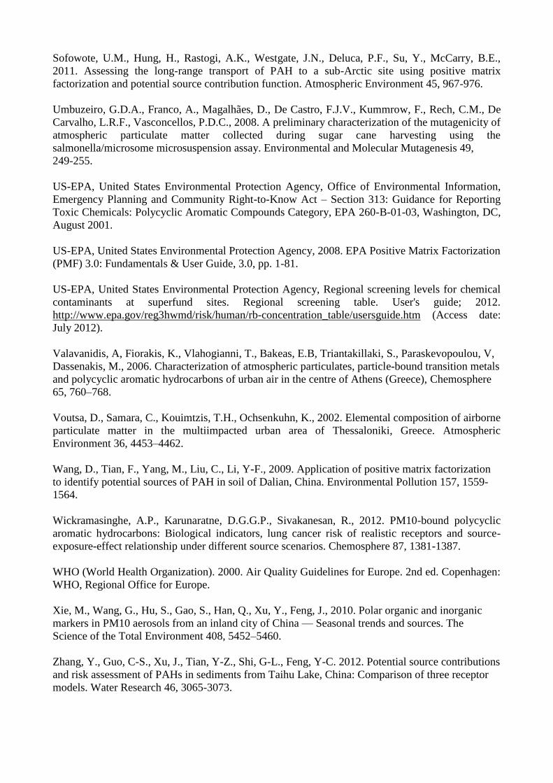
able 2 Mean concentrations and standard deviations (SD) of the four factors obtained by the PMF model, BaP-eq, PM10, total PAH and

meteorological conditions for each cluster obtained by hierarchical cluster analysis (N= number of samples in each cluster).

Coal combustion (ng/m3) Vehicular emissions (ng/m

3)

Cluster A B 1 2 3 4 5 6 7 8 A B 1 2 3 4 5 6 7 8

N 67 17 47 12 4 4 3 4 3 7 67 17 47 12 4 4 3 4 3 7

Mean 0.32 0.65 0.16 0.33 1.20 1.38 1.31 1.32 0.13 0.22 0.32 1.54 0.17 0.68 0.27 1.08 2.50 1.06 1.63 1.37

SD 0.45 0.69 0.16 0.23 0.48 0.86 0.46 0.71 0.19 0.26 0.35 0.61 0.18 0.27 0.21 0.46 0.67 0.47 0.20 0.22

Gasoline emissions (ng/m3) Stationary emissions (ng/m

3)

Cluster A B 1 2 3 4 5 6 7 8 A B 1 2 3 4 5 6 7 8

N 67 17 47 12 4 4 3 4 3 7 67 17 47 12 4 4 3 4 3 7

Mean 0.18 1.02 0.13 0.36 0.30 0.14 0.95 1.80 1.34 0.48 0.16 1.47 0.09 0.37 0.04 0.44 2.70 1.07 1.87 0.99

SD 0.15 0.66 0.08 0.22 0.24 0.03 0.67 0.40 0.30 0.34 0.21 0.76 0.12 0.21 0.10 0.50 0.77 0.27 0.35 0.27

BaP-eq (ng/m3) Total PAH (ng/m

3)

Cluster A B 1 2 3 4 5 6 7 8 A B 1 2 3 4 5 6 7 8

N 67 17 47 12 4 4 3 4 3 7 67 17 47 12 4 4 3 4 3 7

Mean 0.09 0.51 0.05 0.18 0.12 0.29 0.80 0.48 0.64 0.36 1.04 4.69 0.59 1.79 1.88 3.22 7.30 5.14 5.37 3.03

SD 0.09 0.20 0.04 0.05 0.03 0.14 0.19 0.11 0.11 0.10 0.89 1.85 0.34 0.34 0.40 1.56 1.83 1.18 0.61 0.45

PM10 (g/m3) BaP (ng/m

3)

Cluster A B 1 2 3 4 5 6 7 8 A B 1 2 3 4 5 6 7 8

N 67 17 47 12 4 4 3 4 3 7 67 17 47 12 4 4 3 4 3 7

Mean 34.7 33.1 30.1 36.9 75.3 42.2 46.9 15.5 29.4 38.7 0.05 0.26 0.02 0.09 0.05 0.14 0.45 0.24 0.30 0.18

SD 31.5 16.4 16.8 15.9 114.5 28.6 10.4 13.0 21.6 9.7 0.04 0.11 0.02 0.03 0.01 0.08 0.11 0.06 0.03 0.06

Wind direction (º) T (ºC)

Cluster A B 1 2 3 4 5 6 7 8 A B 1 2 3 4 5 6 7 8

N 67 17 47 12 4 4 3 4 3 7 67 17 47 12 4 4 3 4 3 7

Mean 231 158 234 198 239 284 107 217 141 154 15.7 5.6 18.1 11.4 10.6 5.4 3.2 3.1 5.8 8.1

SD 69 64 64 83 94 27 34 76 9 62 7.4 3.5 6.6 4.7 9.6 4.2 1.5 0.7 2.3 3.9

Rainfall (mm) Relative humidity (%)

Cluster A B 1 2 3 4 5 6 7 8 A B 1 2 3 4 5 6 7 8

N 67 17 47 12 4 4 3 4 3 7 67 17 47 12 4 4 3 4 3 7

Mean 0.06 0.01 0.06 0.04 0.07 0.00 0.01 0.00 0.00 0.01 61 81 60 65 58 68 85 74 81 82

SD 0.19 0.01 0.21 0.08 0.13 0.01 0.01 0.01 0.00 0.02 11 12 10 12 17 4 12 14 5 15

Solar radiation (W/m2) Wind Speed (m/s)

Cluster A B 1 2 3 4 5 6 7 8 A B 1 2 3 4 5 6 7 8

N 67 17 47 12 4 4 3 4 3 7 67 17 47 12 4 4 3 4 3 7

Mean 222 98 247 163 169 150 106 78 100 105 3.8 1.7 3.8 3.2 5.4 5.1 1.3 2.6 1.4 1.5

SD 88 64 84 74 57 50 58 28 3 94 2.6 1.0 2.6 2.3 4.3 1.0 0.2 1.9 0.5 0.5

Figure 1. Location of the sampling point at Zaragoza (Spain). The main highway: A-2

and some roads: Z-30, Z-40 as well as different industrial parks are remarked.

I.P.= Industrial parks, WWT= water treatment plant

a)

b)

c)

d)

Figure 2. PMF receptor model applied to total PAH samples in Zaragoza, a)

contribution of sources (ng/m3 and percentage) for the whole sampling

campaign, b) for the cold season, c) for the warm season and d) source

profiles for the PMF four factors. The solid bars represent the amount of each species apportioned to the factor

and the dots line represent the total of each PAH obtained experimentally.

0

0.2

0.4

0.6

0

30

60

90

120

150

180

210

240

270

300

330

Coal combustion

-0.5

0

0.5

1

1.5

2

2.5

1.2

.20

10

6.2

.20

10

11

.3.2

01

0

7.4

.20

10

12

.4.2

01

0

7.5

.20

10

9.6

.20

10

5.7

.20

10

10

.7.2

01

0

5.8

.20

10

14

.9.2

01

0

19

.9.2

01

0

8.1

0.2

01

0

10

.11

.20

10

13

.12

.20

10

18

.12

.20

10

13

.1.2

01

1

Tota

l P

AH

(ng/m

3)

0

0.5

10

30

60

90

120

150

180

210

240

270

300

330

0

0.2

0.4

0.6

0.80

30

60

90

120

150

180

210

240

270

300

330

Gasoline emissions

0

0.5

1

1.5

2

2.5

1.2

.20

10

6.2

.20

10

11

.3.2

01

0

7.4

.20

10

12

.4.2

01

0

7.5

.20

10

9.6

.20

10

5.7

.20

10

10

.7.2

01

0

5.8

.20

10

14

.9.2

01

0

19

.9.2

01

0

8.1

0.2

01

0

10

.11

.20

10

13

.12

.20

10

18

.12

.20

10

13

.1.2

01

1

To

tal

PA

H (

ng

/m3)

0

0.2

0.4

0.60

30

60

90

120

150

180

210

240

270

300

330

Stationary emissions

-0.5

0

0.5

1

1.5

2

2.5

3

3.5

1.2

.20

10

6.2

.20

10

11

.3.2

01

0

7.4

.20

10

12

.4.2

01

0

7.5

.20

10

9.6

.20

10

5.7

.20

10

10

.7.2

01

0

5.8

.20

10

14

.9.2

01

0

19

.9.2

01

0

8.1

0.2

01

0

10

.11

.20

10

13

.12

.20

10

18

.12

.20

10

13

.1.2

01

1

To

tal P

AH

(n

g/m

3)

Figure 3. Time-resolved source contributions (ng/m3) for the four factors apportioned by the

PMF model (right) and the conditional probability function for each factor (left): dot

lines in blue colour for the cold season; dot lines in red colour for the warm season.

0.00E+00

1.00E-05

2.00E-05

3.00E-05

4.00E-05

5.00E-05

6.00E-05

7.00E-05

8.00E-05

0

0.5

1

1.5

2

2.5

3

Cluster 1 Cluster 2 Cluster 3 Cluster 4 Cluster 5 Cluster 6 Cluster 7 Cluster 8

Lif

eti

me

can

cer

ris

k

Fact

or

con

trib

uti

on

Coal combustion

Vehicular emis.

Gasoline emis.

Stationary emis.

Lifetime cancer risk

Figure 4. Plot of the average contribution (ng/m3) of each factor resolved by the PMF

model to the different clusters obtained by the cluster analysis. The dots line

represents the average lifetime cancer risk for each cluster and it is represented

on the right vertical axes based on a URBaP=8.7 x 10-5

ng/m3.