HAL Id: hal-01360024https://hal.archives-ouvertes.fr/hal-01360024

Preprint submitted on 5 Sep 2016

HAL is a multi-disciplinary open accessarchive for the deposit and dissemination of sci-entific research documents, whether they are pub-lished or not. The documents may come fromteaching and research institutions in France orabroad, or from public or private research centers.

L’archive ouverte pluridisciplinaire HAL, estdestinée au dépôt et à la diffusion de documentsscientifiques de niveau recherche, publiés ou non,émanant des établissements d’enseignement et derecherche français ou étrangers, des laboratoirespublics ou privés.

Natural Steganography: cover-source switching forbetter steganography

Patrick Bas

To cite this version:Patrick Bas. Natural Steganography: cover-source switching for better steganography. 2016. �hal-01360024�

1

Natural Steganography:cover-source switching for better steganography

Patrick Bas

Abstract—This paper proposes a new steganographic schemerelying on the principle of “cover-source switching”, the keyidea being that the embedding should switch from one cover-source to another. The proposed implementation, called NaturalSteganography, considers the sensor noise naturally present inthe raw images and uses the principle that, by the addition ofa specific noise the steganographic embedding tries to mimic achange of ISO sensitivity. The embedding methodology consistsin 1) perturbing the image in the raw domain, 2) modeling theperturbation in the processed domain, 3) embedding the payloadin the processed domain. We show that this methodology is easilytractable whenever the processes are known and enables to embedlarge and undetectable payloads. We also show that alreadyused heuristics such as synchronization of embedding changesor detectability after rescaling can be respectively explained byoperations such as color demosaicing and down-scaling kernels.

I. INTRODUCTION

Image steganography consists in embedding a undetectablemessage into a cover image to generate a stego image, theapplication being the transmission of sensitive information.As Cachin proposed in [1], one theoretical approach proposedfor steganography is to minimize a statistical distortion, andthe author proposes to use the Kullback-Leibler divergence.It is interesting to note that this line of research has beenrarely used as a steganographic guideline with few notableexceptions such as model-based steganography [2] whichmimics the Laplacian distributions of DCT coefficients duringthe embedding, HUGO [3] whose model-correction mode triesto minimize the difference between the model of the coverimage and the stego image, and more recently the mi-podsteganographic scheme [4] which minimizes a statistical dis-tortion (a deflexion coefficient) between normal distributionsof cover and stego contents.

Currently the large majority of steganographic algorithmsare based on the use of a distortion (also called a cost) whichis computed for each pixel, and which is combined witha coding scheme that minimizes the global distortion whileembedding a given payload. Classical distortions functionssuch as the ones proposed by S-UNIWARD [5] or by HILL [6]try to infer the detectability of each pixel by assigning smallcosts to pixels that are difficult to predict (usually texturalparts of the image) and by assigning large costs to pixelsthat are easy to predict (belonging to homogeneous areasand to some extend to edges). Note that a recent trend ofresearch [7], [8] proposes to correlate embedding changes onneighboring pixels by adjusting the cost w.r.t the history of theembeddings performed on disjoint lattices in order to decreasethe detectability on greyscale images or on color images [9].

Once the distortion is computed, a steganographic schemecan either simulate the embedding by sampling according to

the modifications probabilities πk, k ∈ [1, . . . , Q] for a Q-arry embedding, or can directly embed the message usingSyndrome Trellis Codes (STCs) [10] or multilayer STCs [10],[11]. The size of the embedding payload N is computed asN =

∑πk log πk for each pixel of the image, and in practice

the STCs succeed to reach 90% to 95% of the capacity [10]and consequently are close to optimal.

Another ingredient to tend to undetectable steganographyis to use the information contained in a “pre-cover”, i.e. thehigh resolution image that is used to generate the cover at alower resolution, in order to weight the cost w.r.t the roundingerror. For quantization or interpolation operations, a pixel ofthe pre-cover at equal distance between two quantization cellswill have a lower cost than a pre-cover pixel very close toone given quantization cell. This strategy has been used inPerturbed-Quantization [12] but also adapted in more recentschemes using side information [13].

The proposed paper uses similar ingredients shared by mod-ern steganographic methods, namely model-based steganogra-phy, Q-arry embedding and the associated modification prob-abilities πk, and side-information. The main originality of thispaper relies on the possible definitions of cover sources andthe use of cover-source switching to generate stego contentswhose statistical distributions are very close to cover contents.

A. What’s a source?

If the term “source” has been first coined with the problemof “cover-source mismatch” after the BOSS contest [14], [15]in order to denote poor steganalysis performances whenevera steganalyzer was trained with an image database comingfrom a set of “sources” and tested on another set. In this casethe term “source” was associated with a camera device, andother authors [16] have associated a “source” with a “user”that would upload a set of pictures on a sharing platform suchas FlickR.

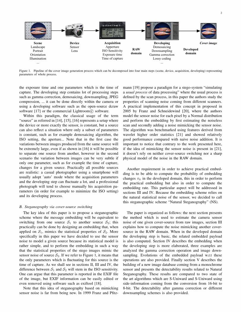
We argue here that a source can be defined w.r.t. the imagegeneration process depicted in Figure 1 which shows thatthe creation of a cover image is linked to the interventionof different parameters represented by (1) the scene that iscaptured, (2) the device which is used, (3) the acquisitionsettings used during the capture and (4) the developing step.

Each parameter is linked with a set of sub-parameters. Thescene fluctuates according to the subject, but also accordingto the illumination or the orientation of the camera. Thedevice is composed mainly of two elements: the sensor (whichcan be CMOS, CDD, color or monochrome) and the lens.The acquisition phase relies on three parameters originatingfrom the device: the lens aperture, the ISO sensitivity and

arX

iv:1

607.

0782

4v1

[cs

.MM

] 2

6 Ju

l 201

6

2

SceneLandscape

PortraitOrientationIllumination

...

DeviceSensorLens

AcquisitionApperture

ISO SensitivityExposure time

Time of capture

DevelopingDemosaicing

DownsamplingGamma correction

Lossy coding...

Cover image

RAW domain

Developed domain

Figure 1. Pipeline of the cover image generation process which can be decomposed into four main steps (scene, device, acquisition, developing) representingparameters of whole process.

the exposure time and one parameters which is the time ofcapture. The developing step contains lot of processing stepssuch as gamma correction, demosaicing, downsampling, JPEGcompression, ... it can be done directly within the camera orusing a developing software such as the open-source dcrawsoftware [17] or the commercial Lightroom c© software.

Within this paradigm, the classical usage of the term“source” as referred in [14], [15], [16] represents a setup wherethe device or more exactly the sensor, is constant, but a sourcecan also reflect a situation where only a subset of parametersis constant, such as for example demosaicing algorithm, theISO setting, the aperture... Note that in the first case thevariations between images produced from the same source willbe extremely large, even if as shown in [16] it will be possibleto separate one source from another, however in the secondscenario the variation between images can be very subtle ifonly one parameter, such as for example the time of capture,changes for a given source. Practically all possible sourcesare realistic: a casual photographer using a smartphone willusually adopt ’auto’ mode where the acquisition parametersand the developing step can fluctuate a lot, and a professionalphotograph will tend to choose manually his acquisition pa-rameters (in order for example to minimize the ISO setting)and its developing process.

B. Steganography via cover-source switching

The key idea of this paper is to propose a steganographicscheme where the message embedding will be equivalent toswitching from one source S1 to another source S2; thispractically can be done by designing an embedding that, whenapplied on S1, mimics the statistical properties of S2. Morespecifically in this paper we have decided to use the sensornoise to model a given source because its statistical model israther simple, and to perform the embedding in such a waythat the statistical properties of the stego images mimic thesensor noise of source S2. If we refer to Figure 1, it means thatthe only parameters which is fluctuating for this source is thetime of capture. As we shall see in sections II, III and IV, thedifference between S1 and S2 will stem in the ISO sensitivity.One can argue that this parameter is reported in the EXIF fileof the image, but EXIF information can be easily edited oreven removed using software such as exiftool [18].

Note that this idea of steganography based on mimickingsensor noise is far from being new. In 1999 Franz and Pfitz-

mann [19] propose a paradigm for a stego-system “simulatinga usual process of data processing” where the usual process isdefined by the scan process, in this paper the authors study theproperties of scanning noise coming from different scanners.A practical implementation of this concept in proposed in2005 by Franz and Schneidewind [20], where the authorsmodel the sensor noise for each pixel by a Normal distributionand perform the embedding by first estimating the noiselessscan and secondly adding a noise mimicking the sensor noise.The algorithm was benchmarked using features derived fromwavelet higher order statistics [21] and showed relativelygood performance compared with naive noise addition. It isimportant to notice that contrary to the work presented here,if the idea of mimicking the sensor noise is present in [21],it doesn’t rely on neither cover-source switching nor a sharpphysical model of the noise in the RAW domain.

Another requirement in order to achieve practical embed-ding is to be able to compute the probability of embeddingchanges πk in the developed domain, this in order to performthe practical embedding but also in order to compute theembedding rate. This particular aspect will be addressed insections III and IV. Because the embedding scheme relies onthe natural statistical noise of the sensor, we decided to callthis steganographic scheme “Natural Steganography” (NS).

The paper is organized as follows: the next section presentsthe method which is used to estimate the camera sensornoise of one given cover-source from raw images, section IIIexplains how to compute the noise mimicking another cover-source in the RAW domain. When in the developed domainthe developing step is basic, the related embedded payloadis also computed. Section IV describes the embedding whenthe developing step is more elaborated, three examples areanalyzed the gamma correction operation and image down-sampling. Evolutions of the embedded payload w.r.t theseoperations are also provided. Finally section V describes thebuilding of a new image database coming from a monochromesensor and presents the detectability results related to NaturalSteganography. These results are compared to two state ofthe art algorithms which are S-Uniward and S-Uniward usingside-information coming from the conversion from 16-bit to8-bit. The detectability after gamma correction or differentdownsampling schemes is also provided.

3

C. Notations

- Capital letters will denote random variables, bold letterdenote vectors or matrices whenever explicitly mentioned.

- Indexes (i, j) will usually denotes the location of thephoto-site1 or the pixel in a given image, and the index kdenotes a modification +k on the cover image. Note that theseindexes will be omitted if not necessary for the formula.

- Notation a denotes the version of a after the developingstep. Each element of respectively the raw cover and theraw stego are denoted xi,j and yi,j and each element of thedeveloped cover and the developed stego are then denotedxi,j and yi,j . The sensor noise is denoted ni,j , and the stegosignals in the raw domain and in the developed domain arerespectively denoted si,j and si,j . The virtual noiseless rawsignal is denoted E[Si,j ] = µ. The probability of adding k onpixel or photo-site si,j is denoted πi,j,k = Pr[Si,j = k].

- The 2D convolution between a matrix m and a filter f isdenoted m ? f .

II. SENSOR NOISE ESTIMATION AND DEVELOPINGPIPELINE

We present in this section the different noises affecting thesensor during a capture and then explain how to estimatethe sensor noise. The last subsection summarizes the imagedeveloping pipeline.

A. Sensor noise model

Camera sensor noise models have been extensively studiedin numerous publications [22], [23], [24] and have alreadybeen used in image forensics for camera device identifica-tion [25], [26]. These models can only be applied to linearsensors such as CDD or CMOS sensors, but this encompassthe majority of modern digital cameras at the date the paperis written. A camera sensor is decomposed into a 2D arrayof photo-sites and the role of each photo-site is to convert kpphotons hitting its surface during the exposure time into a digit.The conversion involves the quantum efficiency of the sensormeasuring the ratio between kp and the number of charge unitske accumulated by the photo-site during the exposure time. keis then converted into a voltage, which is amplified by a gainK (where K is referred as the system overall gain [24]) andthen quantized.

For each photo-site at location (i, j), the converted signalx(i, j) originates from two components:• The “dark” signal xd(i, j) with expectation E[Xd(i, j)] =µd which accounts for the number of electrons presentwithout light and depends on the exposure time andambient temperature,

• The “electronic” signal xe(i, j) with expectationE[Xe(i, j)] = Kµe, which accounts for the number ofelectrons originating from photons coming from the scenewhich is captured.

The expectation µ of each photo-site response is equal to:

1a photo-site denotes the sensor elementary unit, that after demosaicing anddeveloping (without geometrical transforms) generates a pixel.

µi,j = E[X(i, j)] = E[Xd(i, j)] + E[Xe(i, j)] = µd +Kµe.(1)

Beside the signal components, there are three types of noiseaffecting the acquisition:

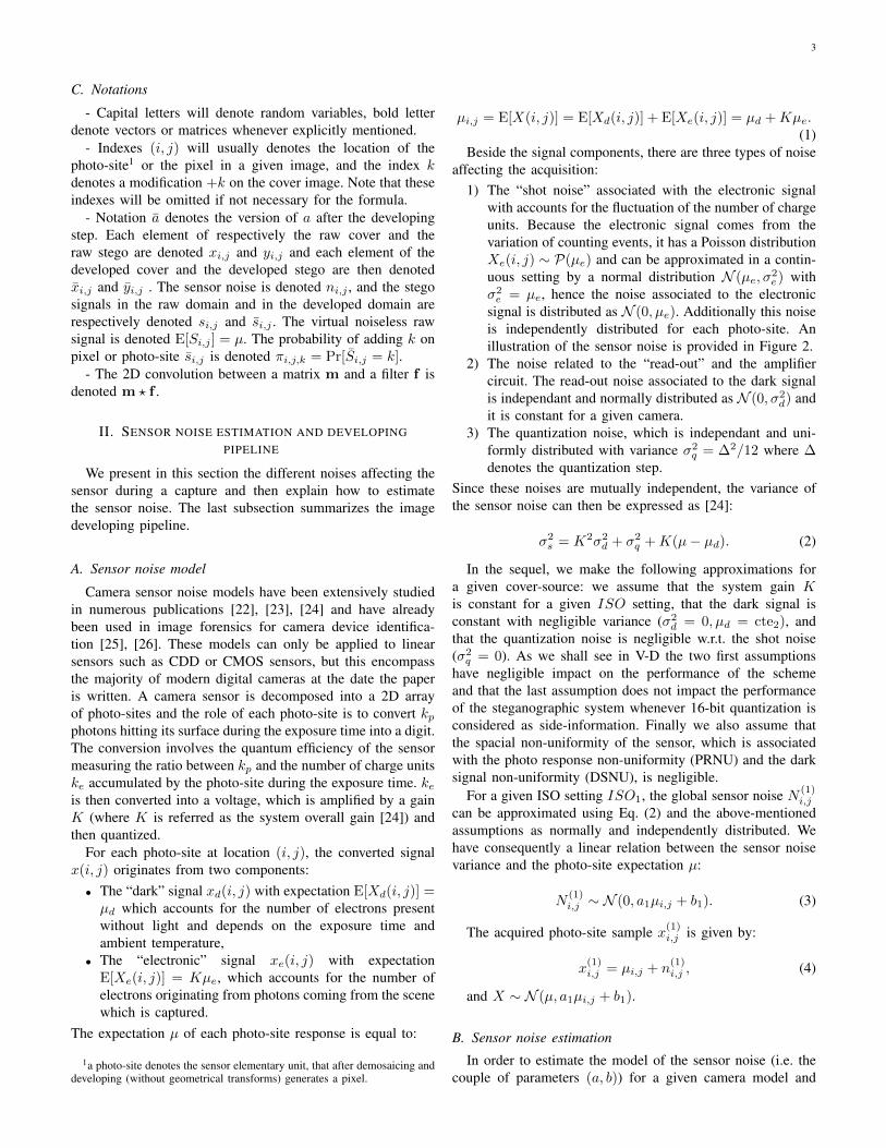
1) The “shot noise” associated with the electronic signalwith accounts for the fluctuation of the number of chargeunits. Because the electronic signal comes from thevariation of counting events, it has a Poisson distributionXe(i, j) ∼ P(µe) and can be approximated in a contin-uous setting by a normal distribution N (µe, σ

2e) with

σ2e = µe, hence the noise associated to the electronic

signal is distributed as N (0, µe). Additionally this noiseis independently distributed for each photo-site. Anillustration of the sensor noise is provided in Figure 2.

2) The noise related to the “read-out” and the amplifiercircuit. The read-out noise associated to the dark signalis independant and normally distributed as N (0, σ2

d) andit is constant for a given camera.

3) The quantization noise, which is independant and uni-formly distributed with variance σ2

q = ∆2/12 where ∆denotes the quantization step.

Since these noises are mutually independent, the variance ofthe sensor noise can then be expressed as [24]:

σ2s = K2σ2

d + σ2q +K(µ− µd). (2)

In the sequel, we make the following approximations fora given cover-source: we assume that the system gain Kis constant for a given ISO setting, that the dark signal isconstant with negligible variance (σ2

d = 0, µd = cte2), andthat the quantization noise is negligible w.r.t. the shot noise(σ2q = 0). As we shall see in V-D the two first assumptions

have negligible impact on the performance of the schemeand that the last assumption does not impact the performanceof the steganographic system whenever 16-bit quantization isconsidered as side-information. Finally we also assume thatthe spacial non-uniformity of the sensor, which is associatedwith the photo response non-uniformity (PRNU) and the darksignal non-uniformity (DSNU), is negligible.

For a given ISO setting ISO1, the global sensor noise N (1)i,j

can be approximated using Eq. (2) and the above-mentionedassumptions as normally and independently distributed. Wehave consequently a linear relation between the sensor noisevariance and the photo-site expectation µ:

N(1)i,j ∼ N (0, a1µi,j + b1). (3)

The acquired photo-site sample x(1)i,j is given by:

x(1)i,j = µi,j + n

(1)i,j , (4)

and X ∼ N (µ, a1µi,j + b1).

B. Sensor noise estimation

In order to estimate the model of the sensor noise (i.e. thecouple of parameters (a, b)) for a given camera model and

4

Figure 2. Illustration of the sensor noise n on a picture at 2000 ISO capturedwith the Leica Monochrome camera. Inactivate the interpolation process ofyour pdf viewer for correct rendering. The pixel amplitudes are scaled forvizualisation purposes.

a given ISO setting, we adopt a similar protocol as the oneproposed in [23].

We first capture a set of Na raw images of a printed photopicturing a rectangular gradian going from full black to white.The camera is mounted on a tripod and the light is controlledusing a led lightning system in a dark room. The raw imagesare then converted to PPM format (for color sensor) or toPGM format (for B&W sensor) using the dcraw open-sourcesoftware [17] using the command:

dcraw -k 0 -4 file_name

which signify that the dark signal is not automaticallyremoved (option -k =0), and that the captured photo-sitesare not post-processed and plainly converted to 16-bit (option-4).

In order to have a process independant of the quantiza-tion, the photo-site outputs are first normalized by dividingthem by ymax = 216 − 1. The range of possible outputsis divided into 1/δ segments of width δ. Each normalizedphoto-site location is assigned to one subset of photo-sitesS` according to its empirical expectation over the acquiredimages ηi,j =

(∑Nal=1 y

(l)i,j/ymax

)/Na. The subset index is

` = [ηi,j/δ] where [.] denotes the integer rounding operation.Once the segmentation into subsets is performed, the empiricalmean is:

µ` =1

|S`|

|S`|∑i=1

S`(i), (5)

where S`(i) denotes the value of a photo-site belonging tothe subset S` and |.| denotes the cardinal of a set.

The unbiased variance associated to each subset as:

σ2` =

1

|S`| − 1

|S(`)|∑i=1

(S`(i)− µ`)2. (6)

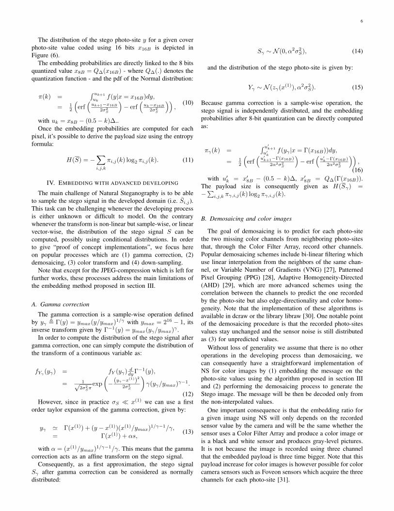
As an illustration, Figure (3) plots the relation in solid linesbetween µ` and σ2

` for Na = 20 raw images captured with a

Leica M Monochrome Type 230 at 1000 ISO and 1250 ISOfor δ = 5 10−5.

The last step consists in estimating the parameters (a, b),this is done by linear regression σ2

N = f(µ) = aµ + b. Wesee on the same figure that the linear relation, depicted by thedashed lines, is rather accurate.

2 3 4 5 6 7

µ 1e 1

1

2

3

4

5

6

7

8

9

σ2 N

1e 5

ISO 1250, measurements

ISO 1000, measurements

ISO 1250, model

ISO 1000, model

Figure 3. Sensor noise estimation for the Leica Monochrome camera and1000 IS0 and 1250 ISO on normalized images. The estimated coefficientsof the linear model are respectively (a1, b1) = (8.36 10−5, 1.11 10−6) and(a2, b2) = (10.46 10−5, 1.95 10−6) for this setup.

C. The developing pipeline

Scene Raw image(12-14bits/channel)

Demosaicing(float or 16bits)

Color transform(float or 16bits)

JPEG(8bit/channel)

Processing/ Geometrical transforms

(float or 16bits) PNG(8bit/channel)

Gamma correction(float or 16bits)

Figure 4. The image developing pipeline.

Since the goal of any steganographic scheme is to embedmessage on a published image and not a raw one, we recallbriefly in this subsection the different steps leading to the gen-eration of a developed picture. The image developing pipeline,depicted on Figure 4 will be further used in sections III and IV.

In a raw image each photo-site is usually represented using12 or 14 bits per channel depending on the sensor bit depth,and most of the color digital cameras only record one colorcomponent per photo-site. Depending of the computationalpower the following process can be performed either usingeither double, float or unsigned integer 16-bit precision.

The first step consist in interpolating for each photo-site thetwo missing color components via the demosaicing process(see also section sub:Demosaicing-and-color). This processcan be linear or non-linear.

5

Scene Raw image(12-14bits/channel)

Demosaicing(float or 16bits)

Color transform(float or 16bits)

JPEG(8bit/channel)

Processing/ Geometrical transforms

(float or 16bits) PNG(8bit/channel)

Gamma correction(float or 16bits)

Figure 5. The basic developing pipeline associated to a monochrome sensor.

A color transform is then applied, and converts the originalcamera color domain to the reference domain XYZ (this trans-form depends on the camera make) and then to a color spacesuch as sRGB, adobe RGB, wide RGB, ... The white balancecorrection can also performed at this stage. All the colorconversion operations can be expressed as multiplications by3× 3 matrices and are consequently linear.

The color components are then corrected using the classicalgamma correction y = x1/γ which is a non-linear sample-wisetransform.

The next step encompasses a large set of possible processingoperations and consists in processing the image by applyingfor example local contrast enhancement, denoising, addinggrain, changing the contrast, ... and applying geometricaltransforms such as cropping, image rescaling (up-sampling ordown-sampling), rotation, lens-distortion compensation, ...

The last step of this pipeline consists in exporting the imagein a lossy compressed format such as JPEG or a lossless formatsuch as PNG, in each case a quantization to 8-bit/channel isperformed.

Note that depending on developing software which is used,this pipeline can be completely known whenever the softwaresource code is public, or unknown if the software is private,but this does not mean for the last case that the processingoperation cannot be reverse-engineered.

III. EMBEDDING FOR OOC MONOCHROME PICTURES

We first propose in this section a steganographic systempractically working for a basic developing setup, this systemis realistic for a monochrome sensor where nor demosaicingneither color transform is possible. As depicted in Figure 5,we also assume that the developed images do not undergogamma correction or further processing and only suffer 8-bitquantization. We can call this type of images “Out Of Camera”(OOC) Pictures. In the next section we show how to deal withmore advanced developing processes.

A. Principle of the embedding

We propose to model the stego signal Si,j is such a way thatit mimics the model of images captured at ISO2 > ISO1.

Based on the assumptions made in II-A, the equivalent of (3)and (4) for a camera sensitivity parameter ISO2 are N (2)

i,j ∼N (0, a2µi,j + b2) and x(2)

i,j = µi,j + n(2)i,j .

Since the sum of two independent noises normally dis-tributed is normal with the variances summing up, we canwrite that x(2)

i,j = µi,j + n(1)i,j + s′i,j = x

(1)i,j + s′i,j with

S′i,j ∼ N (0, (a2 − a1)µi,j + b2 − b1) representing the noisenecessary to mimic image captured at ISO2.

Assuming that the observed photo-site is very close toits practical expectation, i.e. that µi,j ' x

(1)i,j , x(2)

i,j can beapproximated by:

x(2)i,j ' x

(1)i,j + si,j , yi,j , (7)

with:

Si,j ∼ N (0, (a2 − a1)x(1)i,j + b2 − b1), (8)

adopting the following notations a′ , a2− a1, b′ , b2− b1, σ2

S , a′x(1)i,j + b′, and the photo-site of the stego image is

distributed as:

Yi,j ∼ N (x(1)i,j , σ

2S). (9)

Note that equation (7) shows explicitly the principle ofcover-source switching which is simply represented in thiscase by adding an independant noise on each image photo-site to generate the stego photo-site yi,j . The distribution ofthe stego signal in the continuous domain (see (8)) takes intoaccount the statistical model of the sensor noises estimated fortwo ISO settings using the procedure presented in section II-A.

B. 16-bit to 8-bit quantization

For OOC images, the only developing process lies in the8-bit quantization function, consequently the goal here isto compute the embedding changes probabilities πi,j(k) =Pr[Si,j = k] after this process.

These probabilities can be either used to simulate optimalembedding, or cost additive costs ρi,j can be derived andused to feed a multilayered Syndrome Trellis Code usingthe “flipping lemma” [10] as ρi,j = ln (πi,j/(1− πi,j)) withπi,j = max {πi,j , 1− πi,j} (see also section VI of [10] forQ-ary embedding and multi-layered constructions).

x8B − 1 x16B x8B x8B + 1

∆

f(y|x= x16B)

π(0)

π(− 1)

π(1)

Figure 6. Computation of the embedding probabilities after 8-bit quantiza-tion.

We use the high resolution continuous assumption givenby (10) and then we compute the discretized probability massfunction after a quantization step of size ∆ (typically ∆ = 256by quantizing from 16-bit resolution to 8-bit resolution).

6

The distribution of the stego photo-site y for a given coverphoto-site value coded using 16 bits x16B is depicted inFigure (6).

The embedding probabilities are directly linked to the 8 bitsquantized value x8B = Q∆(x16B) - where Q∆(.) denotes thequantization function - and the pdf of the Normal distribution:

π(k) =´ uk+1

ukf(y|x = x16B)dy,

= 12

(erf(uk+1−x16B

2σ2S

)− erf

(uk−x16B

2σ2S

)),

(10)

with uk = x8B − (0.5− k)∆..Once the embedding probabilities are computed for each

pixel, it’s possible to derive the payload size using the entropyformula:

H(S) = −∑i,j,k

πi,j(k) log2 πi,j(k). (11)

IV. EMBEDDING WITH ADVANCED DEVELOPING

The main challenge of Natural Steganography is to be ableto sample the stego signal in the developed domain (i.e. Si,j).This task can be challenging whenever the developing processis either unknown or difficult to model. On the contrarywhenever the transform is non-linear but sample-wise, or linearvector-wise, the distribution of the stego signal S can becomputed, possibly using conditional distributions. In orderto give “proof of concept implementations”, we focus hereon popular processes which are (1) gamma correction, (2)demosaicing, (3) color transform and (4) down-sampling.

Note that except for the JPEG-compression which is left forfurther works, these processes address the main limitations ofthe embedding method proposed in section III.

A. Gamma correction

The gamma correction is a sample-wise operation definedby yγ , Γ(y) = ymax(y/ymax)1/γ with ymax = 216 − 1, itsinverse transform given by Γ−1(y) = ymax(yγ/ymax)γ .

In order to compute the distribution of the stego signal aftergamma correction, one can simply compute the distribution ofthe transform of a continuous variable as:

fYγ (yγ) = fY (yγ) ddyΓ−1(y),

= 1√2σ2Sπ

exp

(− (yγ−x(1))

2

2σ2S

)γ(yγ/ymax)γ−1.

(12)However, since in practice σS � x(1) we can use a first

order taylor expansion of the gamma correction, given by:

yγ ' Γ(x(1)) + (y − x(1))(x(1)/ymax)1/γ−1/γ,= Γ(x(1)) + αs,

(13)

with α = (x(1)/ymax)1/γ−1/γ. This means that the gammacorrection acts as an affine transform on the stego signal.

Consequently, as a first approximation, the stego signalSγ after gamma correction can be considered as normallydistributed:

Sγ ∼ N (0, α2σ2S), (14)

and the distribution of the stego photo-site is given by:

Yγ ∼ N (zγ(x(1)), α2σ2S). (15)

Because gamma correction is a sample-wise operation, thestego signal is independently distributed, and the embeddingprobabilities after 8-bit quantization can be directly computedas:

πγ(k) =´ u′

k+1

u′k

f(yγ |x = Γ(x16B))dy,

= 12

(erf(u′k+1−Γ(x16B)

2α2σ2S

)− erf

(u′k−Γ(x16B)

2α2σ2S

)),

(16)with u′k = x′8B − (0.5 − k)∆, x′8B = Q∆(Γ(x16B)).

The payload size is consequently given as H(Sγ) =−∑i,j,k πγ,i,j(k) log2 πγ,i,j(k).

B. Demosaicing and color images

The goal of demosaicing is to predict for each photo-sitethe two missing color channels from neighboring photo-sitesthat, through the Color Filter Array, record other channels.Popular demosaicing schemes include bi-linear filtering whichuse linear interpolation from the neighbors of the same chan-nel, or Variable Number of Gradients (VNG) [27], PatternedPixel Grouping (PPG) [28], Adaptive Homogeneity-Directed(AHD) [29], which are more advanced schemes using thecorrelation between the channels to predict the one recordedby the photo-site but also edge-directionality and color homo-geneity. Note that the implementation of these algorithms isavailable in dcraw or the library libraw [30]. One notable pointof the demosaicing procedure is that the recorded photo-sitesvalues stay unchanged and the sensor noise is still distributedas (3) for unpredicted values.

Without loss of generality we assume that there is no otheroperations in the developing process than demosaicing, wecan consequently have a straightforward implementation ofNS for color images by (1) embedding the message on thephoto-site values using the algorithm proposed in section IIIand (2) performing the demosaicing process to generate theStego image. The message will be then be decoded only fromthe non-interpolated values.

One important consequence is that the embedding ratio fora given image using NS will only depends on the recordedsensor value by the camera and will be the same whether thesensor uses a Color Filter Array and produce a color image oris a black and white sensor and produces gray-level pictures.It is not because the image is recorded using three channelthat the embedded payload is three time bigger. Note that thispayload increase for color images is however possible for colorcamera sensors such as Foveon sensors which acquire the threechannels for each photo-site [31].

7

C. Color transform

The color transform is a linear operation and consequentlythe 3 components of the stego signal after demosaicing[sCR, sCG, sCB ]T can be expressed as: sR

sGsB

=

c11 c12 c13

c21 c22 c23

c31 c32 c33

sCRsCGsCB

, (17)

where [sR, sG, sB ]T represents the RGB vector after thecolor transform. In the case the color transform does onlywhite balance (ai,j = 0 for i 6= j) we can adopt the samestrategy as in section (IV-B) with SR ∼ N (0, σ2

R , c211σ2SCR

),SG ∼ N (0, σ2

G , c222σ2SSG

), SB ∼ N (0, c2B , c233σ2SSB

).The embedding probabilities and message length computedusing (10) and (11) using σ2

S = σ2S{R,G,B}.

For a classical color transform, we have to proceed dif-ferently and we propose here a sub-optimal scheme thatwill embed a payload only on half on the pixels2 and fordemosaicing that predicts components only from photo-sitescoding the same component (like bilinear demoisaicing):

1) We start by adding a noise distributed as the stego signalon the photo-sites recording the blue and red channels.This noise is not used to convey a message and onlyenable cover-source switching.

2) We interpolate the blue and red components of the sensornoises sCR and sSB for all photo-sites recording thegreen channel using demosaicing.

3) We have then sR = cte1 +c12sCG, sG = cte2 +c22sCG, sB = cte3 + c32sCG and we select the componentCmax ∈ {R,G,B} associated to the highest cmax = ci2to carry the payload. Usually it is also the green compo-nent of the new space. We do so in order to maximizethe embedding capacity of the scheme.

4) We compute the embedding probabilities using (10) withthe appropriate σ2

S′ = c2maxσ2Cmax and we modify the

component accordingly, embedding the payload usingSTCs or simulating embedding.

5) We draw a random variable distributed according to theportion of the gaussian distribution where k is selectedin the previous step (see figure (6)),

6) We compute the modifications on the two other compo-nents ({(R,G,B)−Cmax}) by quantizing the random-variable according to the resolution.

7) We interpolate the other green raw component usingdemosaicing and we perform the color transform onphoto-sites coding R and B.

8) The payload is decoded by reading the values of thecolor channel C on developed photos-sites encoding thegreen information.

It is important to notice that this embedding process will bringa positive correlation between color components whenevercmax and the ci2 of the selected component are of same sign,and a negative correlation otherwise. Note that the idea offorcing correlation between embedding changes has already

2This is because the information is carried on green photo-site which on abayer CFA represents half of the photo-sites.

empirically been proposed in a variation of CMD for colorimages [9], we bring here a more theoretical insight of whythis is necessary.

D. Down-sampling (and up-sampling)

We propose in this subsection strategies to deal with imagedown-sampling. We restrict our analysis to integer down-scaling factors c ∈ N+.

Note that upscaling with integer factors is the similarstrategy than the one of demosaiced images since the predictedpixels are constructed from the non-interpolated ones and donot carry any information. As a consequence an up-sampledimage carrie the same payload than the original one.

For down-sampling we distinguish three strategies: sub-sampling, box down-sampling and down-sampling usingconvolutional kernels such as tent down-sampling.

1) Sub-sampling: Sub-sampling consists in selecting pixelsdistant by kc pixels (k ∈ N+) on each column and rowof the image. For a stationary image, naïve sub-samplingconsequently does not modify the average embedding rate,but this sub-sampling method is rarely used in practice sinceit creates aliasing.

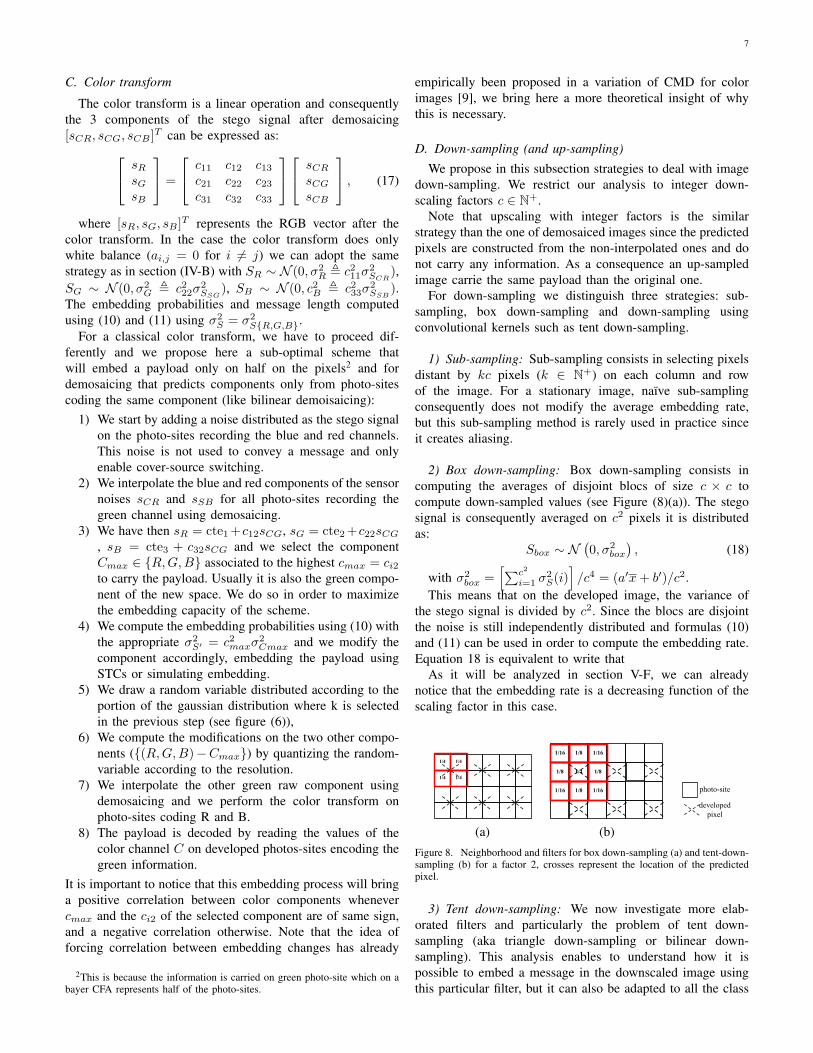
2) Box down-sampling: Box down-sampling consists incomputing the averages of disjoint blocs of size c × c tocompute down-sampled values (see Figure (8)(a)). The stegosignal is consequently averaged on c2 pixels it is distributedas:

Sbox ∼ N(0, σ2

box

), (18)

with σ2box =

[∑c2

i=1 σ2S(i)

]/c4 = (a′x+ b′)/c2.

This means that on the developed image, the variance ofthe stego signal is divided by c2. Since the blocs are disjointthe noise is still independently distributed and formulas (10)and (11) can be used in order to compute the embedding rate.Equation 18 is equivalent to write that

As it will be analyzed in section V-F, we can alreadynotice that the embedding rate is a decreasing function of thescaling factor in this case.

1/4

1/4

1/4

1/4

1/16

1/8

1/161/8

1/4

1/8

1/16

1/8

1/16

photo-site

developedpixel

(a) (b)Figure 8. Neighborhood and filters for box down-sampling (a) and tent-down-sampling (b) for a factor 2, crosses represent the location of the predictedpixel.

3) Tent down-sampling: We now investigate more elab-orated filters and particularly the problem of tent down-sampling (aka triangle down-sampling or bilinear down-sampling). This analysis enables to understand how it ispossible to embed a message in the downscaled image usingthis particular filter, but it can also be adapted to all the class

8

of linear filters, including for example the Gaussian kernel orthe Lanczos kernel [32].

E1

E2

E3

E4

Figure 9. Embedding steps used for tent-down sampling: dark grey photo-sites are sampled during the first step, light grey photo-sites during the secondstep and white photo-sites during the last step.

As for color transform, we propose an embedding schemethat we believe is sub-optimal, i.e. that does’t convey themaximum payload but that ensures that the stego signalmimics correctly the sensor-noise. Without loss of generalitythe principle of the embedding scheme is explained for c = 2and in this case the tent filter and down-sampling process isillustrated on Figure 8(b).

This method starts by decomposing the down-scaled pixelsinto four disjoint lattices and associated subsets. Note that theembedding strategy is then similar to the ones designed tounable synchronization between embedding changes such asthe “CMD” strategy or the “Sync” strategy [7], [8].

This decomposition is done in order to obtain developedpixels for which the stego signal is independently distributedconditionally to the neighborhood. On figure 8(b) we can seethat the first and second developed pixels (represented bycrosses) are not independant since 3 photo-sites contribute tothe computation of both pixels, on the contrary the first andthird pixels of the first row are independant.

The embedding procedure can be decomposed into foursteps, each of them associated to a given subset of photo-sites.

In this section we adopt the following notations: indexesi, j are centered on the pixel to develop ({−1, 0, 1} representsrespectively {1, 2, 3} rows or columns), and the tent filteris denoted as a 3 × 3 matrix with coefficient ci,j . The fourdifferent subsets {E1, E2, E3, E4} of photo-sites are represented

on Figure 9. Moreover↑s,↓s,←s and

→s denotes stego signal

added on the photo-sites related to neighboring developedpixels according to the ↑, ↓,←,→ directions. As an exampleit means that s−1,0 =

↑s1,0.

The embedding is sequentially performed in 4 steps:1) The first step embeds part of the message (or generate

the stego signal) into pixels belonging to E1. Because thesubset E1 generates independent pixels, the stego signalin the developed domain is distributed as:

N (0, σ2S1), (19)

with σ2S1 =

∑1i,j=−1 c

2i,jσ

2S(i, j). Applying results

of III, one can compute the embedding probabilities, andthe associated payload length associated to the pixelsbelonging to E1. In order to be able to sample theneighboring pixels, once an embedding change is done,we draw realizations of the 9 underlying photo-sites.

This can be done by computing conditional probabilitiesor performing rejection sampling.

2) Developed pixels belonging to E2 have a sensornoise distributed according to the conditional densityf(s|←s i−1,1,

←s i,1,

←s i+1,1,

→s i−1,1,

→s i,1,

→s i+1,1) and con-

sequently can be expressed as:

N (µS2, σ2S2), (20)

with µS2 =∑1i=−1 ci,1

←s i,1 +

∑1i=−1 ci,−1

→s i,−1 and

σ2S2 =

∑1i=−1 c

2i,0σ

2S(i, 0). As for the first step, we

can compute embedding probabilities and payload lengthfor this subset. We can also draw the realizations ofstego signal related to the 3 photo-sites belonging tothis subset. Note that the same applies for steps 3 and4.

3) Similarly pixels belonging to E3 have a sensor noise aredistributed as:

N (µS3, σ2S3), (21)

with µS3 =∑1j=−1 c1,j

↑s1,j +

∑1j=−1 c1,j

↓s1,j and

σ2S3 =

∑1j=−1 c

20,jσ

2S(0, j), and as for step 2, it is

possible to draw realizations of the stego signal.4) An finally, pixels belonging to E4 have a sensor noise

distributed as:

N (µS4, σ2S4), (22)

with µS4 =∑1j=−1 c1,j

↑s1,j +

∑1j=−1 c−1,j

↓s−1,j +

c0,1←s 0,1 + c0,−1

→s 0,−1 and σ2

S4 = c20,0σ2S(0, 0). For this

last step, notice that only one photo-site is drawn.

Note that since H(S|←S i−1,1,

←S i,1,

←S i+1,1,

→S i−1,1,

→S i,1,

→S i+1,1) ≤

H(S), the payload length embedded during steps 4 is smallerthan the payload length embedded during 2 and 3, which issmaller than the payload length embedded during step 1.

V. EXPERIMENTAL RESULTS

The goal of this section is to benchmark the detectabilityof NS, to compare it with other steganographic schemes usingsame embedding payload, but also to analyze the effects ofdeveloping operations w.r.t. both detectability and embeddingrates.

A. Generation of “MonoBase”

In order to benchmark the concept of embedding usingcover-source switching, we needed to acquire different sourcesproviding OOC images. To do so we conducted the followingexperiment: using a Leica M Monochrome Type 230 camera,we captured two sets of 172 pictures taken at 1000 ISO or1250 ISO. In order to have large diversity of contents mostof the pictures were captured using a 21mm lens in a urbanenvironment, or a 90mm lens capturing cluttered places.

The exposure time was set to automatic, with exposurecompensation set to -1 in order to prevent over-exposure.A tripod was used so that pictures for the two sensitivitysettings correspond to the same scene. Each RAW picture

9

was then converted into a 16-bit PGM picture using the sameconversion operation as the one presented in section II-B andeach 5212× 3472 picture was then cropped into 6× 10 = 60PGM pictures of size 512× 512 to obtain two sets of 1032016-bit PGM pictures. We consequently end up with a databaseof a similar size than BOSSBase, with pictures of same sizethat contrary to un-cropped pictures can be quickly processedeither for embedding or feature extraction. This database calledMonoBase is downloadable here [33]. Figure 7 shows severalimages of MonoBase.

B. Benchmark setupFor all the following experiments, we adopt the Spatial

Rich Model feature sets [34] combined with the EnsembleClassifier (EC) [35] and we report the average total errorPE = min((PFA + PMD)/2) obtained after training the ECon 10 different training/testing sets divided in 50/50. The stegodatabase consists of images captured at 1000 ISO perturbedwith an embedding noise mimicking 1250 ISO, and the coverdatabase consists of images captured at 1250 ISO. In order tohave an effect equivalent with the principle of training usingpairs of cover and stego images, the pairs are constructed usingone couple of images capturing the same scene.

The parameters of the stego signal are denoted a” and b”with the relations a” = a′(2Nb − 1) and b” = b′(2Nb − 1)2,where a′ and b′ are computed using normalized image valuesin order to be resolution independant (see section III-A). Nb =16 when the cover image coded in 16-bit is used and Nb =8 when the stego image is directly generated from the 8-bitrepresentation of the cover image.

C. Basic developing and comparison with S-UniwardWe first benchmark the scheme proposed in section III and

generate 8-bit stego images where the stego signal is generatedaccording to the embedding probabilities computed in 10. Likeall the modern steganographic schemes, we forbid embeddingsby attributing wet pixels to cover pixels saturated at 0 or 255.We also propose a variation of NS where the dark pixels,i.e. the pixels of the cover have the lowest value after 8-bitsquantization, are also wet. This strategy, even if developedindependently, is similar to the one recently proposed in [36].For NS, we used the same values that the ones estimated insection II, i.e. a” = 2.1 10−5 and b” = 8.4 10−7.

The two first columns of table I show the high unde-tectability of the proposed scheme, and the small improvementassociated to wet the dark pixels. We note that we are stillaround 7% from random guessing, and we think that it canbe due to the different assumption presented in section III,particularly the fact that the quantization noise is ignored.

NS NS SUni-SI SUni 1000 ISOwo wet dark 1000 ISO 1000 ISO vs 1250 ISO

PE 41.0% 42.8% 18.2% 12.3% 26.0%

Table IRESULTS AND COMPARISON WITH S-UNIWARD ON MONOBASE 1000 ISO.

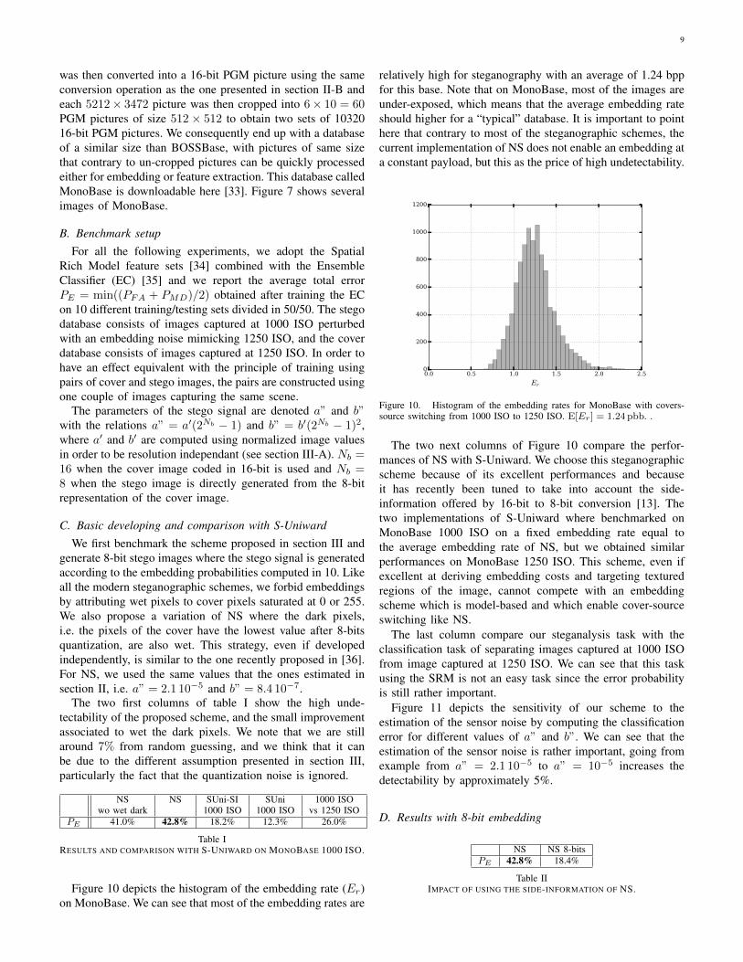
Figure 10 depicts the histogram of the embedding rate (Er)on MonoBase. We can see that most of the embedding rates are

relatively high for steganography with an average of 1.24 bppfor this base. Note that on MonoBase, most of the images areunder-exposed, which means that the average embedding rateshould higher for a “typical” database. It is important to pointhere that contrary to most of the steganographic schemes, thecurrent implementation of NS does not enable an embedding ata constant payload, but this as the price of high undetectability.

0.0 0.5 1.0 1.5 2.0 2.5

Er

0

200

400

600

800

1000

1200

Figure 10. Histogram of the embedding rates for MonoBase with covers-source switching from 1000 ISO to 1250 ISO. E[Er] = 1.24 pbb. .

The two next columns of Figure 10 compare the perfor-mances of NS with S-Uniward. We choose this steganographicscheme because of its excellent performances and becauseit has recently been tuned to take into account the side-information offered by 16-bit to 8-bit conversion [13]. Thetwo implementations of S-Uniward where benchmarked onMonoBase 1000 ISO on a fixed embedding rate equal tothe average embedding rate of NS, but we obtained similarperformances on MonoBase 1250 ISO. This scheme, even ifexcellent at deriving embedding costs and targeting texturedregions of the image, cannot compete with an embeddingscheme which is model-based and which enable cover-sourceswitching like NS.

The last column compare our steganalysis task with theclassification task of separating images captured at 1000 ISOfrom image captured at 1250 ISO. We can see that this taskusing the SRM is not an easy task since the error probabilityis still rather important.

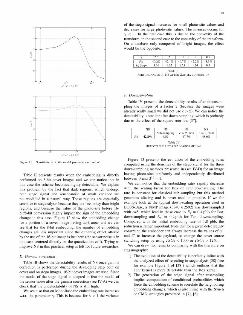
Figure 11 depicts the sensitivity of our scheme to theestimation of the sensor noise by computing the classificationerror for different values of a” and b”. We can see that theestimation of the sensor noise is rather important, going fromexample from a” = 2.1 10−5 to a” = 10−5 increases thedetectability by approximately 5%.

D. Results with 8-bit embedding

NS NS 8-bitsPE 42.8% 18.4%

Table IIIMPACT OF USING THE SIDE-INFORMATION OF NS.

10

10−6 10−5 10−4

a” , b” = 8.4 10−7

0

10

20

30

40

50

PE,%

10−7 10−6 10−5

b” , a” = 2.1 10−5

0

10

20

30

40

50

PE,%

Figure 11. Sensitivity w.r.t. the model parameters a” and b”.

Table II presents results when the embedding is directlyperformed on 8-bit cover images and we can notice that inthis case the scheme becomes highly detectable. We explainthis problem by the fact that dark regions, which undergoboth stego signal and sensor-noise of small variance arenot modified in a natural way. These regions are especiallysensitive to steganalysis because they are less noisy than brightregions, and because the value of the photo-site before 16-bit/8-bit conversion highly impact the sign of the embeddingchange in this case. Figure 12 show the embedding changefor a portion of a cover image having dark areas and we cansee that for the 8-bit embedding, the number of embeddingchanges are less important since the dithering effect offeredby the use of the 16-bit image is lost here (the sensor noise is inthis case centered directly on the quantization cell). Trying toimprove NS in this practical setup is left for future researches.

E. Gamma correction

Table III shows the detectability results of NS once gammacorrection is performed during the developing step both oncover and on stego images. 16-bit cover images are used. Sincethe model of the stego signal is adapted to feat the model ofthe sensor-noise after the gamma correction (see IV-A) we cancheck that the undetectability of NS is still high.

We see also that on MonoBase the embedding rate increasesw.r.t. the parameter γ. This is because for γ > 1 the variance

of the stego signal increases for small photo-site values anddecreases for large photo-site values. The inverses occurs forγ < 1. In the first case this is due to the convexity of thetransform, in the second case to the concavity of the transform.On a database only composed of bright images, the effectwould be the opposite.

γ 2.5 2 1.5 1 0.5PE 40.2% 42.1% 40.7% 42.2% 43.3%

Er(bpp) 1.61 1.62 1.55 1.24 0.5

Table IIIPERFORMANCES OF NS AFTER GAMMA CORRECTION.

F. Downsampling

Table IV presents the detectability results after downsam-pling the images of a factor 2 (because the images werealready really small we did not use c > 2). We can notice thedetectability is smaller after down-sampling, which is probablydue to the effect of the square root law [37].

NS NS NS NSSub-sampling c = 2, Box c = 2, Tent

PE 42.8% 48% 47.7% 48.0%

Table IVDETECTABLY AFTER X2 DOWNSAMPLING.

Figure 13 presents the evolution of the embedding ratescomputed using the densities of the stego signal for the threedown-sampling methods presented in (see IV-D) for an imagehaving photo-sites uniformly and independently distributedbetween 0 and 216 − 1.

We can notice that the embedding rates rapidly decreasew.r.t. the scaling factor for Box or Tent downscaling. Therate is constant for classical sub-sampling but this methodgenerates aliasing and is never used in practice. If we forexample look at the typical down-scaling operation used inBOSS-Base, a 18MP image (3840 x 2592) was downsampledwith c=5, which lead in these case to Er ≈ 0.4 pbb for Boxdownsampling and Er ≈ 0.2 pbb for Tent downsampling.Compared with the initial embedding rate of 1.8 pbb, thereduction is rather important. Note that for a given detectabilityconstraint, the embedder can always increase the values of a”and b” to increase the payload, or change the cover-sourceswitching setup by using ISO1 < 1000 or ISO2 > 1250.

We can draw two remarks comparing with the literature onsteganography:

1) The evolution of the detectability is perfectly inline withthe analyzed effect of rescaling in steganalysis [38] (seefor example Figure 1 of [38]) which outlines that theTent kernel is more detectable than the Box kernel.

2) The generation of the stego signal after resamplingimplies computation of conditional probabilities whichforce the embedding scheme to correlate the neighboringembedding changes, which is also inline with the Synchor CMD strategies presented in [7], [8].

11

1 2 3 4 5 6 7 8 9 10

c

0.0

0.5

1.0

1.5

2.0

Er

Sub-samplingBoxTent

Figure 13. Embedding rate vs scaling factor, 1000 ISO toward 1250 ISOembedding for a cover image uniformly distributed, a′ = 2.1 × 10−5,b′ =8.4× 10−7.

VI. ANOTHER STRATEGY: COVER-SOURCE PERTURBATION

We want to mention alternative strategy to cover-sourceswitching which is cover-source perturbation. In this casethe embedding does not mimic another cover-source but justslightly perturbs it. This can simply done by setting b” = 0,setting a” and comparing cover images with stego imageswith the same sensitivity (here 1000 ISO), this way the stegosignal slightly perturbs the sensor-noise. The advantage ofcover-source perturbation is the fact that is doesn’t require tomodel the source sensor noise which can be very interestingin practice.

We present results related to cover-source perturbation inTable V which depicts the evolution of the detection errorand the embedding w.r.t. a” when both cover images are at1000 ISO. We can notice that cover-source perturbation mayoffer undetectability but at the price of a smaller embeddingrate. For example for the same PE as NS with cover-sourceswitching, the embedding rate is roughly divided by 3.

a” 4 10−7 1.5 10−6 6.3 10−6 2.5 10−5 10−4

PE 46.2% 45.5% 41.4% 24.7% 5.4%Er (bpp) 0.16 0.32 0.63 1.19 1.98

Table VCOVER-SOURCE PERTURBATION, COMPARISON WITH COVERS AT 1000

ISO.

VII. CONCLUSIONS AND PERSPECTIVES

We have proposed in this paper a new methodology forsteganography based on the principle of cover-source switch-ing, i.e. the fact that the embedding should mimics theswitching from one cover-source to another. The scheme wepresented scheme (NS) used the sensor noise to model onesource and message embedding is performed by generatinga suited stego signal which enables the switch. This method,in order to provide good undetectability performances whileproposing high embedding rates, has to use RAW images as

inputs. We also show in the paper how to handle differentsteps of image developing, including quantization, gammacorrection, color transforms and rescaling operations.

In future works we want also to investigate other setupsfor NS steganography, such as choosing other ISO parametersand different camera models. It will also be important to try toimprove direct embedding on 8-bit images and to address morepractical implementation such as embedding in the JPEG-domain.

From the adversary point of view, we would like to see ifmore appropriate feature could be designed for this categoryof schemes, this kind of features should not be sensitive onlyto image variation, but also to the sensor noise whose varianceis function of the pixel luminance.

Another track of research is to consider other ways toperform cover-source switching (or cover-source perturbation,see section VI), where the source can be represented here by,for example, the demosaicing algorithm. Since the behaviorof demosaicing algorithms fluctuates a lot in textures, wethink that this strategy would generate embedding changes thatare closer to the ones used currently by other steganographicmethods.

Finally we hope that this methodology will page the roadfor new directions in steganography.

VIII. ACKNOWLEDGMENTS

The author would like to thank Boris Valet for his workon sensor noise estimation, Cyrille Toulet and Matthieu Mar-quillie for their help on the Univ-lille HPC, Remi Bardenetfor his help on sampling strategies, Tomas Pevny and AndrewKer for their inspiring conversations of the definition of thesource, and CNRS for a supporting grant on cyber-security.

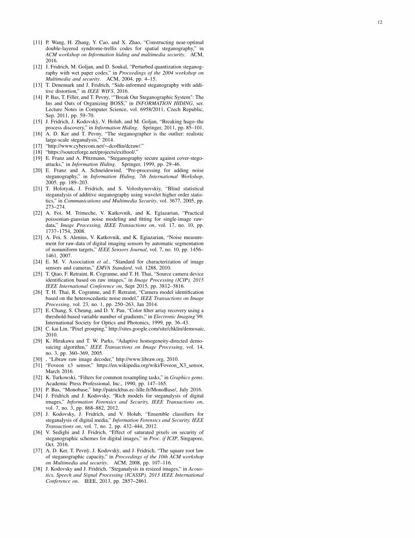
REFERENCES

[1] C. Cachin, “An information-theoretic model for steganography,” inInformation Hiding: Second International Workshop IHW’98, Portland,Oregon, USA, April 1998.

[2] P. Sallee, “Model-based steganography,” in International Workshop onDigital Watermarking (IWDW), LNCS, vol. 2, 2003.

[3] T. Pevny, T. Filler, and P. Bas, “Using high-dimensional image modelsto perform highly undetectable steganography,” in Information Hiding2010, 2010.

[4] V. Sedighi, R. Cogranne, and J. Fridrich, “Content-adaptive steganog-raphy by minimizing statistical detectability,” vol. 11, no. 2, Feb 2016,pp. 221 – 234.

[5] V. Holub, J. Fridrich, and T. Denemark, “Universal distortion functionfor steganography in an arbitrary domain,” EURASIP Journal on Infor-mation Security, vol. 2014, no. 1, pp. 1–13, 2014.

[6] B. Li, M. Wang, J. Huang, and X. Li, “A new cost function forspatial image steganography,” in Image Processing (ICIP), 2014 IEEEInternational Conference on. IEEE, 2014, pp. 4206–4210.

[7] T. Denemark, V. Sedighi, V. Holub, R. Cogranne, and J. Fridrich,“Selection-channel-aware rich model for steganalysis of digital images,”in IEEE Workshop on Information Forensic and Security, Atlanta, GA,2014.

[8] B. Li, M. Wang, X. Li, S. Tan, and J. Huang, “A strategy of clusteringmodification directions in spatial image steganography,” InformationForensics and Security, IEEE Transactions on, vol. 10, no. 9, pp. 1905–1917, 2015.

[9] W. Tang, B. Li, W. Luo, and J. Huang, “Clustering steganographicmodification directions for color components,” 2016.

[10] T. Filler, J. Judas, and J. Fridrich, “Minimizing additive distortion insteganography using syndrome-trellis codes,” Information Forensics andSecurity, IEEE Transactions on, vol. 6, no. 3, pp. 920–935, 2011.

12

[11] P. Wang, H. Zhang, Y. Cao, and X. Zhao, “Constructing near-optimaldouble-layered syndrome-trellis codes for spatial steganography,” inACM workshop on Information hiding and multimedia security. ACM,2016.

[12] J. Fridrich, M. Goljan, and D. Soukal, “Perturbed quantization steganog-raphy with wet paper codes,” in Proceedings of the 2004 workshop onMultimedia and security. ACM, 2004, pp. 4–15.

[13] T. Denemark and J. Fridrich, “Side-informed steganography with addi-tive distortion,” in IEEE WIFS, 2016.

[14] P. Bas, T. Filler, and T. Pevny, “"Break Our Steganographic System": TheIns and Outs of Organizing BOSS,” in INFORMATION HIDING, ser.Lecture Notes in Computer Science, vol. 6958/2011, Czech Republic,Sep. 2011, pp. 59–70.

[15] J. Fridrich, J. Kodovsky, V. Holub, and M. Goljan, “Breaking hugo–theprocess discovery,” in Information Hiding. Springer, 2011, pp. 85–101.

[16] A. D. Ker and T. Pevny, “The steganographer is the outlier: realisticlarge-scale steganalysis,” 2014.

[17] “http://www.cybercom.net/∼dcoffin/dcraw/.”[18] “https://sourceforge.net/projects/exiftool/.”[19] E. Franz and A. Pfitzmann, “Steganography secure against cover-stego-

attacks,” in Information Hiding. Springer, 1999, pp. 29–46.[20] E. Franz and A. Schneidewind, “Pre-processing for adding noise

steganography,” in Information Hiding, 7th International Workshop,2005, pp. 189–203.

[21] T. Holotyak, J. Fridrich, and S. Voloshynovskiy, “Blind statisticalsteganalysis of additive steganography using wavelet higher order statis-tics,” in Communications and Multimedia Security, vol. 3677, 2005, pp.273–274.

[22] A. Foi, M. Trimeche, V. Katkovnik, and K. Egiazarian, “Practicalpoissonian-gaussian noise modeling and fitting for single-image raw-data,” Image Processing, IEEE Transactions on, vol. 17, no. 10, pp.1737–1754, 2008.

[23] A. Foi, S. Alenius, V. Katkovnik, and K. Egiazarian, “Noise measure-ment for raw-data of digital imaging sensors by automatic segmentationof nonuniform targets,” IEEE Sensors Journal, vol. 7, no. 10, pp. 1456–1461, 2007.

[24] E. M. V. Association et al., “Standard for characterization of imagesensors and cameras,” EMVA Standard, vol. 1288, 2010.

[25] T. Qiao, F. Retraint, R. Cogranne, and T. H. Thai, “Source camera deviceidentification based on raw images,” in Image Processing (ICIP), 2015IEEE International Conference on, Sept 2015, pp. 3812–3816.

[26] T. H. Thai, R. Cogranne, and F. Retraint, “Camera model identificationbased on the heteroscedastic noise model,” IEEE Transactions on ImageProcessing, vol. 23, no. 1, pp. 250–263, Jan 2014.

[27] E. Chang, S. Cheung, and D. Y. Pan, “Color filter array recovery using athreshold-based variable number of gradients,” in Electronic Imaging’99.International Society for Optics and Photonics, 1999, pp. 36–43.

[28] C. kai Lin, “Pixel grouping,” http://sites.google.com/site/chklin/demosaic,2010.

[29] K. Hirakawa and T. W. Parks, “Adaptive homogeneity-directed demo-saicing algorithm,” IEEE Transactions on Image Processing, vol. 14,no. 3, pp. 360–369, 2005.

[30] , “Libraw raw image decoder,” http://www.libraw.org, 2010.[31] “Foveon x3 sensor,” https://en.wikipedia.org/wiki/Foveon_X3_sensor,

March 2016.[32] K. Turkowski, “Filters for common resampling tasks,” in Graphics gems.

Academic Press Professional, Inc., 1990, pp. 147–165.[33] P. Bas, “Monobase,” http://patrickbas.ec-lille.fr/MonoBase/, July 2016.[34] J. Fridrich and J. Kodovsky, “Rich models for steganalysis of digital

images,” Information Forensics and Security, IEEE Transactions on,vol. 7, no. 3, pp. 868–882, 2012.

[35] J. Kodovsky, J. Fridrich, and V. Holub, “Ensemble classifiers forsteganalysis of digital media,” Information Forensics and Security, IEEETransactions on, vol. 7, no. 2, pp. 432–444, 2012.

[36] V. Sedighi and J. Fridrich, “Effect of saturated pixels on security ofsteganographic schemes for digital images,” in Proc. if ICIP, Singapore,Oct. 2016.

[37] A. D. Ker, T. Pevny, J. Kodovsky, and J. Fridrich, “The square root lawof steganographic capacity,” in Proceedings of the 10th ACM workshopon Multimedia and security. ACM, 2008, pp. 107–116.

[38] J. Kodovsky and J. Fridrich, “Steganalysis in resized images,” in Acous-tics, Speech and Signal Processing (ICASSP), 2013 IEEE InternationalConference on. IEEE, 2013, pp. 2857–2861.

13

Figure 7. Six samples from MonoBase.

(a) (b) (c)Figure 12. Portion of an image (a) and locations of embedding changes when 16-bit to 8-bit is used (b) and when it is not used (c) (for better rendering,inactivate interpolation on your pdf viewer).