natural resource s: a blessing or a curse ? the role of ... · pdf filenatural resource s: a...

1

Natural Resources: a Blessing or a Curse?

The Role of Inequality

Tullio Buccellato (a) and Michele Alessandrini (b)

October 2009

Abstract

In this paper we offer a novel contribution to the resource curse literature. We offer a theoretical and empirical analysis to establish that natural resources represent per se a positive factor for countries economic development, but can lead to very unequal income distribution within countries due to their inner characteristic of being easily appropriable. We predict theoretically that the gap between households having access to natural resources and those not having access to natural resources becomes even more marked when raw natural resources are directly exported and do not represent an intermediate input for domestic production. Our empirical results suggest that this is particularly the case for metals and ores.

(a) Office for National Statistics, UK. The opinions and views expressed in this paper by the author do not reflect in any way the opinions and views of the ONS as an institution. Corresponding author: [email protected]

(b) Dipartimento di Economia e Istituzioni, Università di Roma Tor Vergata. Email: [email protected]

Discussion Paper 98

Centre for Financial & Management Studies

2

1. Introduction

In the economic literature, the role of natural resources, in particular oil and gas, has been broadly

discussed as having a negative impact on economic prosperity and long run growth (Corden and

Neary 1982, Eastwood and Venables 1982, Corden 1984, Sachs and Warner 1995, et al.). Several

factors can be responsible for the oil curse or the so called Dutch disease. First, the exchange rate

effect through the appreciation of domestic currency induced by natural resources trade; second,

and directly connected with the first, the consequent loss of competitiveness of other domestic

tradable products on the international markets; third, the shift of investments towards traded natural

resources and non-tradable sectors preventing a solid and diversified economic growth.

Among other aspects concerning natural resource trade, the hypothesis of a negative impact

of natural resources through the channel of increased corruption has been considered (Leite and

Weidmann 1999). Natural resources trade can stimulate rent-seeking behaviours that, together with

a highly concentrated bureaucratic power, induce high degree of corruption in the economy and,

hence, lower the quality of institutions. The low level of institution quality has been proved to

represent a heavy constrain for long run growth. More recently, the possible link of increased

dependence on natural resources with both inequality and less rapid growth rates has been

investigated by Gylfason and Zoega (2002). Starting from the empirical finding of an inverse

relation between inequality and growth (Persson and Tabellini 1994, Perotti 1996), the authors

show both theoretically and empirically that inequality can represent the linking factor between the

two variables. Moreover, Buccellato and Michievicz (2009) have established that hydrocarbons

have positively impacted inequality both between and within Russian regions.

Following the contribution of Gylfason and Zoega (2002), in this paper we try to provide a

further perspective to investigate the possible causes of the so-called natural resource curse. Making

use of a dynamic model of endogenous growth adapted for the presence of non-renewable

resources, we try to assess the impact of hydrocarbons trade on inequality and then on growth

patterns. The model is constructed taking into account possible heterogeneity in wealth

accumulation patterns across households. We distinguish between two households types: type 1,

which has no access to the natural resources trade revenues; and type 2, which instead has access to

such a kind of revenues. Holding this assumption, it follows a continuous increase in differences of

accumulated wealth between the two groups. The speed of divergence in accumulated factor is

directly connected with the degree of dependence of the economy on natural resources (represented

by the share of natural resources trade to GDP) and with the dimension of the groups share with

Natural Resources: a Blessing or a Curse? The Role of Inequality

SOAS | University of London

3

respect to the total population. In order to better disentangle the impact of natural resources trade

we normalize the two present value Hamiltonians, for type 1 and type 2 households respectively

(Hartwick 1990). The normalization is implemented by dividing the present value Hamiltonian by

the marginal utility of consumption. Making use of double-entry bookkeeping, implying the

equality between product or expenditure side and income or value-added side, we end up providing

a dynamic measure of natural resources inducing inequality. In other words, we show that

accumulation of wealth has a much higher pace for those households having access to the natural

resources.

We then test some of our theoretical findings through a regression analysis. The empirical

study is based on an unbalanced panel of 122 countries over the period 1980-2004 resulting from

the merge of data from two sources: the World Income Inequality Database (WIID) and the World

Development Indicators. We make use of ores and metals as the variable capturing the effect of

natural resources on inequality dynamics. The choice of ores and metals is motivated by the fact

that the other two natural resources lack data availability – oil and hydrocarbons – or cannot be

considered as inputs of production – agricultural raw materials. Our results suggest that ores and

metals seem to have a clear and significant role in enhancing inequality within countries, and that

the economic dependence on exports of ores and metals widens the gap between the two types of

households.

The structure of the paper is as follows. Section 2 presents and describes the model and its

economic implications on the relationship between natural resources dependence and level of

inequality. Section 3 analyses the level and the evolution of the Gini Index of the countries

composing our sample and investigates the corresponding shares of ores and metals on merchandise

exports; we then test the model described in the previous section on an unbalanced panel over the

period between 1980-2004 by using the fixed-, random- and between-effect econometric

procedures. Section 4 concludes.

2. The Model

We consider an optimal growth open economy with heterogeneous agents and depletable natural

resources. There is a continuum of households, which have identical preferences but differ with

respect to their wealth accumulation patterns. Heterogeneity in wealth accumulation is completely

driven by natural resources revenues, which are controlled only by one group of households. The

Discussion Paper 98


4

aim of this paper is to analyse the effect of natural resource trade on inequality, through the lens of

an accounting system for dynamic economies. We derive the linear, dollar –valued, present value

Hamiltonians for the two households types. In order to do so, we make use of profit intertemporal

arbitrage relations directly derived by the optimization problem faced by households. Finally, we

present an original measure of inequality in the economy represented by the difference of the two

types of input-output tables.

We start by considering a continuous time model in which at each time )t ![0," national

income Y(t) is represented by the sum of firms’ output, produced by using machine capital K(t) and

natural resources O(t), and the exports of natural resources. Natural resources, therefore, can either

be considered as a production factor (with share ! ) or allocated as export on the international

market (with share !"1 ):

1) Y (t) = F(K(t),!O(t)) + (1"! ) j(t)O(t)

where )(tj is the international price of natural resources, which for simplicity is assumed to be

equal to the marginal productivity of oil in the production process of the rest of the world. Domestic

competitive firms maximize the rental rate of capital by r(t):

2) !(t) = F(K(t),"O(t)) # r(t)K(t) #"( j(t)O(t))

The capital market is in equilibrium if

3) )()()( 21 tKtKtK +=

where K1(t) =

n1

n1+ n

2

K(t) , K2(t) = (1!

n1

n1+ n

2

)K(t) and n1+ n

2= n . n

1 represents the number of

households accessing exclusively machine capital and only indirectly the natural resources through

the production process. The remaining part of households, (1!n1

n1+ n

2

) , has instead the possibility

to rely on both the machine capital and the natural resources endowments. Natural resources mainly

refer to the amount of hydrocarbons, ores and metals and any other raw materials present in the

economy and we assume them to be homogeneously distributed across the share of households

owning them. The output market equilibrium condition is:



5

4) )()()()()1())(),(()()(.

tKteOtOtjtOtKFtKtC !"" ###+=+

where )()()1( tOtj!" is the part of natural resources exported and not devoted to the domestic

production process. e and ! represent the extraction cost per unit of natural resource and the rate of

depreciation of machine capital respectively. We denote the remaining stock of natural resources by

S(t). This is extracted at the following rate:

5) )()()(.

tOtStS !=

Households exhibit different patterns of wealth accumulation according to whether they have access

or not to the sector of extraction and trade of natural resources. On the one hand, type 1 households

accumulate wealth by supplying capital to firms:

6)K.

1(t) = r(t)K1(t) ! C1

On the other hand, type 2 households accumulate wealth by supplying both man-made capital and

natural resources:

7) K.

2 (t) = r(t)K2(t) + j(t)O(t) ! C

2

Households choose consumption in order to maximize their lifetime utility subject to their

respective constraints. The present value Hamiltonians are:

8) H1=U(C

1) ! e"#t + $

k(t) ![F(K(t),% !O(t)) " C

1(t)]+ $

o(t)[S "O]

9) H2=U(C

2) ! e"#t + $k (t) ![F(K(t),% !O(t)) + (1"% ) j(t)O(t) " C

2(t)]+ $o(t)[S "O]

where k

! and o

! are costate variables associated with man-made capital and natural resources,

respectively. Next step is to obtain the two present value Hamiltonians normalized by C

U , in order

to express flows in numeraire goods, say dollars (Hartwick 1990). Since the marginal utility of

Discussion Paper 98


6

consumption is the same for the two groups of households1, by using the following linear

approximation

CUCUC!=)( ,

!o(t)

Uc

=!o(t)

!k(t)

we obtain:

10) H1

UC1

= C1! e"#t + [F(K(t),$ !O(t)) " C

1(t)]+

%o(t)

%k(t)[S "O]

11) H2

UC2

= C2! e"#t + [F(K(t),$ !O(t)) + (1"$ ) j(t)O(t) " C

2(t)]+

%o(t)

%k (t)[S "O]

A direct measure of dynamic inequality in income levels can be now derived as the difference

between the two present value Hamiltonians. Let us then introduce our dynamic indicator for

inequality as:

12)I =H2

UC2

!H1

UC1

=

= C2" e!#t + [F(K(t),$ "O(t)) + (1!$ ) j(t)O(t) ! C

2(t)]+

%o(t)

%k (t)[S !O]! C

1" e!#t +

![F(K(t),$ "O(t)) ! C1(t)]!

%o(t)

%k (t)[S !O] =

= C2" e!#t + (1!$ ) j(t)O(t) ! C

2(t) ! C

1" e!#t + C

1(t) =

= (e!#t !1)(C

2! C

1) + (1!$ ) j(t)O(t)

1 From the first order conditions,

!H1

!C1

= 0 and !H

2

!C2

= 0 , we obtain: UC1=U

C2= !

k(t) .



7

The level of inequality, I, is affected by the difference of consumption between the two groups and

by the share of natural resources allocated as export on the international market (for the share

!"1 ). In the long run e!"t → 0, while the two accumulation processes asymptotically converge to

K

.

1(t) = 0 andK.

2 (t) = 0 . As a result, we have that:

13) C1= rK

1

14) C2= rK

2+ jO

By substituting the definition for K1 and K

2 into 13 and 14 and replacing C

1andC

2into 12 we

obtain the formula for the level of inequality in the long run:

15) I =rK

n(n1! n

2) !" jO

The level of inequality is therefore increasing in n1, the part of the population who has access

exclusively to machine capital and only indirectly to the natural resources through the production

process. If therefore fewer people have the control of the revenues of the natural resources, the

distance in terms of inequality between the two groups rises. Moreover, the model predicts that

when ! grows, that is, more natural resources are dedicated to production (and less allocated to

exports), the level of inequality declines. This would suggest that natural resources devoted to

national production tend to be more redistributed through the improved level of generated gross

value added. Such a theoretical finding will be the object of our empirical analysis.

3. Empirical analysis

3.1 Our measure of inequality: the Gini Index

In order to evaluate the level of inequality within countries, we make use of the index of income

concentration, commonly known as the Gini Index. A straightforward graphical interpretation of the

Gini coefficient is in terms of the Lorenz curve, which denotes the area between the horizontal axis

displaying the cumulative percentage of population ordered form the poorest to the richest and the

vertical axis displaying the cumulative percentage of income associated with the population units.

When income distribution is egalitarian, the Lorenz curve coincides with the 45-degree line; as

Discussion Paper 98


8

incomes vary within population, that is, inequality rises, the Lorenz curve moves towards the

bottom right-hand corner. The Gini Index, therefore, measures the differences between the area

under the 45-degree line and the area defined by the Lorenz curve. As a result, the Gini coefficient

will be equal to 0 in the case of perfect equal distribution (no inequality) and approaches to 1 (or to

100%) when only one individual in the population owns the total amount of income (maximum

inequality).

The Gini index provides a useful insight into the levels of actual income distribution within

the states and allows comparing inequality both across countries and over time. However, the

validity of the Gini coefficient depends upon the quality of the statistical data used to calculate it. In

this paper we use the dataset provided by UNU-WIDER for 122 countries for the period from 1980

to 2004. Although this represents the widest available source of data at present, it contains many

missing values in terms of years and/or countries observations, which makes it difficult to compare

and describe countries in terms of inequality for different selected years. In order to overcome this

problem, we calculate, for each country, the average Gini index across all the available observations

for the entire period from 1980 to 2004 and for three different sub-periods, 1980-1989, 1990-1999

and 2000-2004. Even if this method could be affected by the numbers of observations - some

countries display only one observation for each decade – it allows ranking states according to their

level of inequality and studying the evolution of the Gini index across countries. Moreover, changes

in the Gini Index take time to occur and it is therefore very rare to observe a consistent

increase/decrease in the level of inequality in just a few years so that it can affects the average.

3.2 Descriptive analysis

Table 1 ranks the top-bottom 25 countries according to their average Gini Index over the period

from 1980 to 2004 and collects the corresponding (available) averages calculated for the three

different sub-periods. The first part of the table is entirely occupied by African and Latin American

economies, with a predominant presence of the firsts in the top positions (Namibia, Zimbabwe and

Lesotho). Moreover, some big developing economies such as Brazil, South Africa or Mexico

display high levels of inequality. For most Latin American countries, we can compare the evolution

of inequality over time observing that income concentration has practically remained unchanged or,

as in the case of Chile, Bolivia, Ecuador and Paraguay, improved in its value. The lower part of the

table shows countries with the lowest level of inequality, with many high-income European

countries placed in the bottom positions. It is interesting to underline that some economies

composing the collapsed Soviet bloc (at least for what concerns the Central East European



9

countries, this does not apply to countries part of the Commonwealth of Independent States, which

are also more endowed of natural resources), such as Slovak and Czech Republic, Bulgaria or

Latvia have a relative low level of inequality, mainly due to the egalitarianism imposed by the

communist systems to the economies. Furthermore, the Gini index does not consider the size of the

underground economy, which is considerable in the former socialist countries as well as in many

developing countries, hiding income for many and altering the level of inequality either up and

down (Rosser et al., 2000). Moreover, different countries could show different Lorenz curves

despite the same level of the Gini coefficient. This could also explain why United States shows a

notable level of inequality (42.7 on average between 1980-2004), despite the high per-capita

income. However, contrarily to the other countries placed in the bottom part of the tables, inequality

has risen over time in the former socialist economies, and the economic and political transition

towards market-oriented systems has implied a rise in the unequal distribution of income.

The second step of this descriptive analysis is to investigate, according to the model, the

relationship between the level of inequality and natural resources abundance. We use data on ores

and metals exports as a proxy of the natural resources using the dataset provided by the World

Development Indicators (WDI 2007). This variable appears to be the most indicated in testing our

model. The use of oil and hydrocarbons products, in fact, induce a bias in our estimations due to the

lack of data concerning the Gini index of the Middle-East countries, leaders in the worldwide oil

production; moreover, raw agricultural materials, although considered as part of natural resources

(see the data appendix in the WDI 2007), cannot be regarded as proper production or industrial

inputs. We therefore consider the percentage of total merchandise exports dedicated to ores and

metals. A high share of ores and metals over total exports implies a “dependence” of the economy

on it, and, if the control on the extraction activities and the related revenues does not ensure an

adequate distribution across population of the benefits guaranteed by the abundance of that

resource, could lead to an increase in the income concentration and a rise in the level of inequality.

We combine the exercise conducted to construct the previous tables with the average of each

country across the ores and metals shares over different periods. This allow us to compare the

average level of inequality with the average levels of ores and metals exports over total

merchandise exports, in order to establish whether a country which shows high inequality registers

also a high share of ores and metals exports.

Table 2 summarizes the results, by dividing, for each period, the sample of countries into

four quartiles according to the level of inequality (high, medium-high, medium-low and low). Due

to the insufficient availability of observations especially on the Gini Index, the number of

Discussion Paper 98


10

economies considered in each inequality group varies over decades. However, some revealing

aspects emerge from the Table. First of all, the group with the highest level of inequality shows also

the highest level, on average, in the ores and metals share in all the periods considered; the average

weight of ores and metals exports for this group is 14.7% for the entire period, with the highest

value recorded in the 1990s (15.8%). Second, countries in the low-inequality quartile also display a

lower impact of ores and metals on the composition of exports. Finally, the two groups representing

the medium levels of inequality show also a medium level of natural resource dependence.

However, it has to be noted that in the 1990s and between 2000 and 2004, the medium-low group in

terms of inequality exhibits a higher share of ores and metals with respect to the medium-high

quartile. This aspect, although influenced by the different numbers of countries composing each

group in the four periods, needs further investigations, in order to identify which countries have a

share of ores and metals exports higher than the corresponding level of inequality.

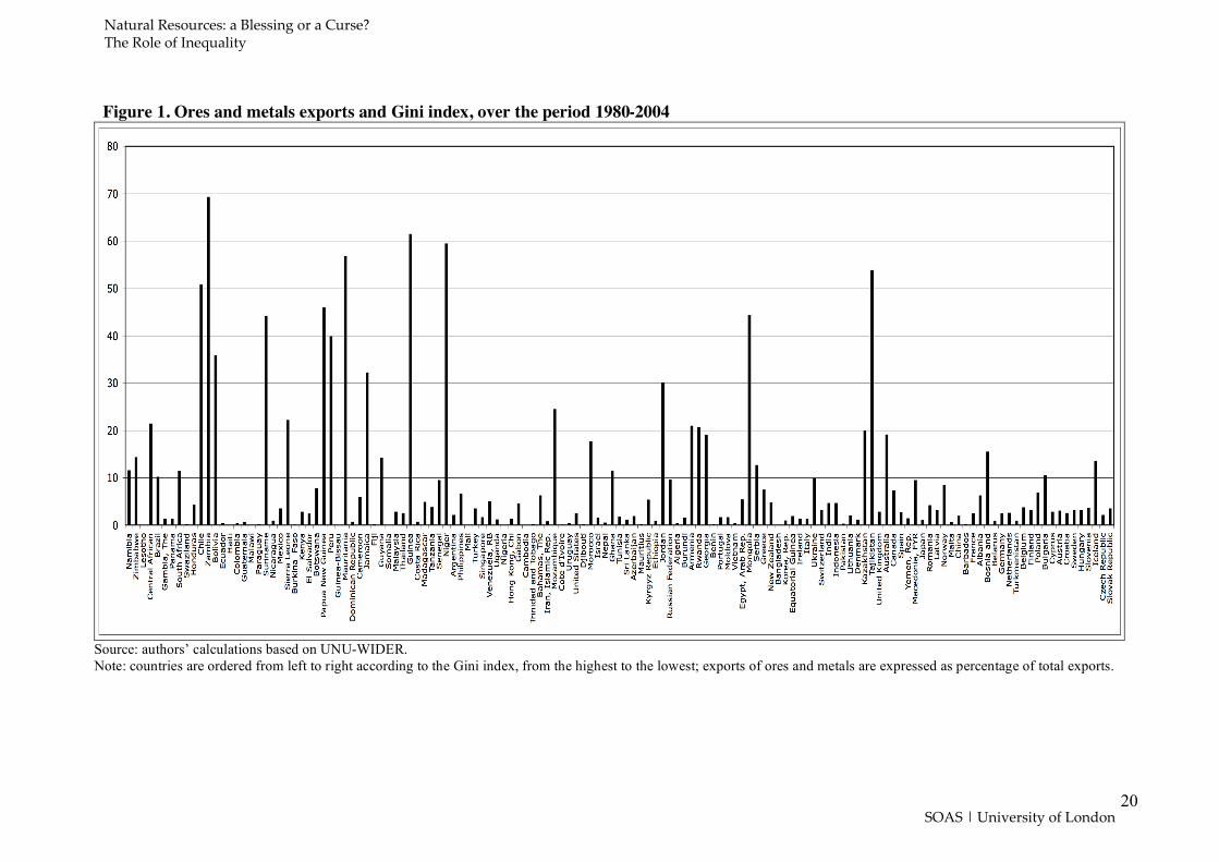
Figures from 1 to 4 order countries form left to right according to the Gini Index, from the

highest to the lowest. The vertical axis measures the share of ores and metals exports over total

merchandise exports. These Figures illustrate the relationship between inequality and ores and

metals abundance for the overall period and for the three sub-periods 1980-1989, 1990-1999 and

2000-2004. Figures 1 shows that the countries with the highest levels of ores and metals exports are

mainly concentrated in the left half of the horizontal axis (high level of inequality), although

accompanied by the presence of economies with a share of exports close to 0. Many African

countries together with Latin American economies present a notable dependence on natural

resources coupled with a high level of inequality: in the case of Chile, Zambia, Mauritania and

Guinea, the weight of ores and metals represents more than half of total exports between 1980 and

2004. Some other economies, like Peru or Bolivia, show a level of exports more than one third of

total exports. The lowest quartile in terms of Gini Index is composed by ten countries out of 35 with

a share of ores and metals over the 20% of total exports. By contrast, the left part of the horizontal

axis contains countries with a low level of inequality and a low share of ores and metals exports:

only two countries, Kazakhstan and Tajikistan, reach the 20% of total exports with the last economy

up to more than 50%. The majority of the group has a share of ores and metals below 5%. Finally,

among the seventy economies composing the two middle-inequality quartiles, only six display a

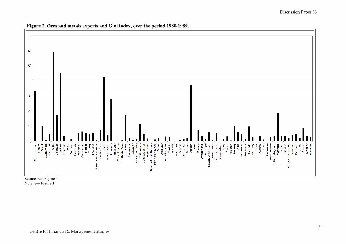
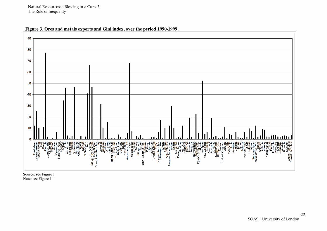
share of ores ad metals in excess of one fifth of total exports. In the following Figures 2, 3 and 4 the

number of countries changes according to the availability of data, but the main observations carried

out for the previous Figure 1 are confirmed, with the concentration of resource-abundant economies

among the countries with the highest level of inequality.



11

3.3 Regression analysis

To test whether income distribution is affected by natural resources, we make also use of panel data

regression analysis. For this purpose we construct a model whose dependent variable is always the

Gini Index and independent variable the share of export represented by ores and metals. In

formula:

)1(_ ,,,10, titititiXresourcesNaturalGINI !"## +++=

where ti

X,

is a matrix in which we gradually add some more control variables to account for

various country specific characteristics, which may affect income distribution. ! is the vector of

coefficients associated with the control variables. The number of countries included in each

regression ranges from a minimum of 68 to a maximum of 122, depending on the number of

observations for each of the new regressors gradually added. The time span of the panel is 1980-

2004, but with gaps resulting in an unbalanced panel.

The first control variable that we include is the GDP. This variable allows us to control

simultaneously for many specific characteristics of the countries and also partially for its size. We

then add up the population to control for demographic size effects. Both GDP and population are

transformed in logarithms. Already adding these two control variables we should have a relatively

clear and unbiased interpretation of the relation linking income distribution and natural resources

and hence we can label the results obtained through this specification as our “core” results. We

complete our analysis by adding to our “core” model two more variables. We first add the share of

export to GDP. This allows us to further clean the coefficient of our natural resources variables

from possible effects of openness and attraction of hard currency. Finally, we add a variable

representing the share of people enrolled in the secondary school as a proxy for the access to

education infrastructures. Overall, considering also that we estimate all our panel data specifications

in three ways – random effect, fixed effect and between effect - we end up estimating 15 regression

specifications ordered in Table 3. Implementing the three different methodologies allows us to

exploit at best all the dimensions of our dataset exploiting the between (between effect estimator),

the within (fixed effect estimator) and both dimensions (random effect) of the dataset. This also

allows us to have more terms of comparison when it comes to comment on the significance and

robustness of our results.

Discussion Paper 98


12

Our results seem to establish quite clearly that ores and metals are positively related to

income inequality. The variable turns out indeed to be very significant in the majority of

specifications, and, even when not significant, always with the expected sign. When implementing

the fixed effect panel data analysis, even though the sign of ores and metals confirms that

dependence on trade of natural resources tends to exacerbate the level of inequality across courts in

the economy, the level of significance is generally low (in the order of 10%) or completely

inexistent as in the case of the specification without control variables or when adding our proxy for

access to education infrastructures. Results become more stable and easy to interpret when

considering the random effect. The coefficient linked with ores and metals is indeed not only

always positive but also very significant, oscillating between 1% and 5% significance level. The

between effect represents somehow a synthesis between the fixed and the random effects with

results more significant than the former and less than the latter. Overall, it should to be also noticed

that ores and metals is the only variable of the model that exhibits stability in sign and is on average

the more significant in determining the level of inequality within countries. Finally, assuming that

fixed effects estimates are consistent, we implement the Hausman test to establish which is the

preferable estimation procedure between fixed and random effects. In all cases it turns out that the

preferable estimation procedure is the fixed effect methodology.

In addition to testing the relation of inequality with exports of ores and metals we have also

implemented a regression analysis considering quantities of hydrocarbons extracted by countries.

At this stage of our research we have decided to omit to report our results because of the complete

lack of data for the Middle East. With Saudi Arabia being one of the world leaders in oil

production, and many other important countries with an extremely high share of hydrocarbons

revenue to the overall economy, we suspect that our results could change substantially if we had

Gini Index data for those countries.

4. Conclusions

The presence and the abundance of a natural resource in a country could generate positive

spillovers for an economy, by reducing production costs or favouring revenues from international

trade. However, empirical evidence suggests that economies endowed with natural resources have

grown slower than other economies and that they persist, in many cases, in a poverty trap condition.

Furthermore, economic dependence on natural resources could affect income not only in terms of

level or growth, but also regarding its distribution across population units within countries. In fact,



13

when the control of the revenues from natural resources and their extraction process is concentrated

in a few households, the abundance of natural resources could raise inequality in the income

distribution. As a result, high concentration of natural resources implies concentration of income.

Following this hypothesis, we have constructed a dynamic model of endogenous growth in

order to establish the impact of natural resources exports on income accumulation and thus on

inequality. By assuming a distinction among households based on the control of the revenues from

the natural resources exports, we show that there is a positive relation between inequality and

dependence on natural resources. We have then tested the validity of our model by using data on the

Gini Index and on ores and metals exports for an unbalanced panel of countries from 1980 to 2004.

Our results confirm the hypothesis depicted in the model and countries displaying a higher level of

ores and metals exports show also a higher level of income inequality.

Discussion Paper 98


14

References

Aghion, P. and Commander, S. (1999) “On the Dynamics of Inequality in the Transition”, Economics of Transition, Vol. 7, No. 2, pp. 275-298.

Aghion, P., Caroli, E. and Garcia-Penelosa, E. (1999), “Inequality and Economic Growth: The Perspective of New Growth Theory,” Journal of Economic Literature, Vol 37, No. 4, pp. 1615-1660.

Alesina A. and Perotti R. (1996), ” Income distribution, political instability, and investment,” European Economic Review, Vol. 40, No. 6, pp. 1203–1228.

Alessandrini M. and Enowbi Batuo M. (2008), “The Trade Specialization of Sane: Evidence from Manufacturing Industries”, CeFiMS Discussion Paper No. 91, SOAS, University of London.

Arellano M. and Bond S. (1991), “Some tests of specification for panel data: MonteCarlo Evidence and an Application to employment equations,” Review of Economic Studies, Vol. 58, No. 2, pp. 277-297.

Buccellato T. and Micievicz T.M. (2009), “Oil and Gas: A Blessing for the Few. Hydrocarbons and Inequality within Regions in Russia”, Europe-Asia Studies, Vol. 61, No. 3., pp. 385-407.

Caselli F., Esquivel, G. and Lefort F.(1996), “Reopening the Convergence Debate: A New Look at Cross-Country Growth Empirics”, Jurnal of Economic Growth, Vol. 1, No. 3, pp. 363-389.

Commander S., A. Tolstopiatenko, and R.Yemtsov (1999), “Channel of Redistribution-Inequality and poverty in the Russian transition” The Economics of Transition, Vol. 7, No. 2, pp. 411-447

Conceição P. and.Galbraith J. K (2000), “Constructing Long and Dense Time Series of InequalityUsing the Theil Statistic”, Eastern Economic Journal, Vol. 26, No. 1, pp. 61-74.

Corden W. M. and J. Peter Neary (1982), “Booming Sector and De-Industrialisation in a Small Open Economy,” The Economic Journal, Vol. 92, No. 368. pp. 825-848.

Corden W. M. (1984), “Booming Sector and Dutch Disease Economics: Survey and Consolidation”, Oxford Economic Papers, New Series, Vol. 36, No. 3. pp. 359-380.

Eastwood R. K. and Venables A. J. (1982), “The Macroeconomic Implications of a Resource Discovery in an Open Economy,” The Economic Journal, Vol. 92, No. 366. pp. 285-299.

Ellman, M. (2006), Russia's Oil and Natural Gas - Bonanza or Curse?, Anthem Press.

Forbes K. (2000), “A Reassessment of the Relationship Between Inequality and Growth,” American Economic Review, Vol. 90, No. 4, pp. 869–886.

Gaddy C. G. and. Ickes B. W (2005), “Resource Rents and the Russian Economy,” Eurasian Geography and Economics, Vol. 46, No. 8, pp. 559–583.



15

Galbraith J. K., L. Krytynskaia and Q. Wang (2003), “The Experience of Rising Inequality in Russia and China during the Transition,” The European Journal of Comparative Economics, Vol. 1, No. 1, pp. 87-106.

Gylfason T. and G. Zoega (2002), “Inequality and Economic Growth: Do Natural Resources Matter?,” CESifo Working Paper, No. 712 (5), April.

Gerry C. J. and T. Mickiwicz (2007), “Inequality, Democracy and Taxation: Lessons from the Post-Communist Transition,” UCL – SSEES Economics Working Paper, No. 74, March.

Hartwick J,M, (1990), “Natural Resources, National Accounting and Economic Depreciation”, Journal of Public Economics, Vol. 43, pp. 291-304.

Kronenberg T. (2004), “The Curse of Natural Resources in the Transition Economies,” Economics of Transition, Vol. 12, No. 3, pp. 399–426.

Kuznets, S. (1995), “Economic Growth and Income Inequality”, American Economic Review, Vol. 45, No. 1, pp. 1-28.

Kuznets, S. (1963),” Quantitative Aspects of the Economic Growth of Nations”, Economic Development and Cultural Change, Vol. 11, pp. 1-80.

Leite C. and J. Weidman (1999), “Does Mother Nature Corrupt? Natural Resources, Corruption, and Economic Growth,” IMF Working Paper, WP/99/85.

Li H. and H. Zou (1998), “Income Inequality is not Harmful for Growth: Theory and Evidence,” Review of Development Economics, Vol. 2, No. 3, pp. 318–334.

Milanovic B. (1999), Explaining the Increase in Inequality During Transition, The Economics of Transition, Vol. 7, p. 299.

Perotti R. (1996), “Growth, Income Distribution, and Democracy: What the Data Say”, Journal of Economic Growth, Vol. 1, No. 2, pp. 149–187.

Persson T. and G. Tabellini (1994), “Is inequality harmful for growth?,” American Economic Review, Vol. 84, No. 3, pp. 600–621.

Reilly B. (1999), The Gender pay gap in Russia during the transition, 1992-96, The Economics of Transition, Vol. 7, p. 245.

Rosser, J. B, Rosser, M. V. and Ahmed, E. (2000) “Income Inequality and the Informal Economy in Transition Economies”, Journal of Comparative Economics, Vol. 28, No. 1, pp. 156-171.

Sachs D.J. and A.M.Warner (2001), “Natural Resources and Economic Development-The Curse of Natural Resources”, European Economic Review, Vol. 45, pp. 827-838.

Sukiassyan G. (2007), “Inequality and Growth: What Does the Transition Economy Data Say?,” Journal of Comparative Economics, Vol. 35, No. 1, pp. 35–56.

Discussion Paper 98


16

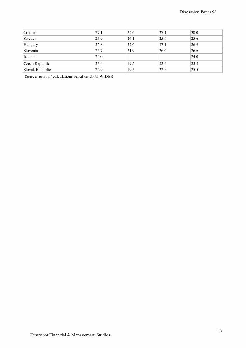
Table 1. Gini index, top-bottom according to 1980-2004 average

Country 1980-2004 1980-1989 1990-1999 2000-2004 Namibia 73.9 73.9 Zimbabwe 64.9 64.9 Lesotho 60.6 58.9 61.7 Central African Republic 60.4 60.4 Brazil 58.4 58.2 58.8 58.1 Gambia, The 57.6 57.6 Panama 55.3 51.3 55.7 56.3 South Africa 54.9 47.0 60.4 56.5 Swaziland 54.8 59.2 50.4 Honduras 54.4 55.7 54.1 54.4 Chile 54.4 54.3 54.2 56.0 Zambia 54.4 58.3 46.5 Bolivia 54.2 52.0 54.2 55.8 Ecuador 54.1 44.1 54.5 60.2 Haiti 53.9 51.5 55.1 Colombia 53.7 49.5 55.9 56.2 Guatemala 53.6 56.0 51.3 52.9 Malawi 53.5 58.6 55.7 39.0 Paraguay 53.1 45.1 51.7 56.9 Suriname 52.8 52.8 Puerto Rico 52.7 50.2 55.1 52.9 Nicaragua 52.2 54.0 48.5 Mexico 51.5 48.4 52.9 51.6 Sierra Leone 51.4 63.7 39.0 Burkina Faso 51.0 54.8 39.5 Latvia 30.2 24.9 30.4 34.0 Norway 30.1 32.1 29.2 29.3 Malta 30.0 30.0 China 29.9 23.8 31.2 39.9 Barbados 29.9 29.9 France 29.7 33.4 29.6 27.6 Albania 29.5 29.3 29.6 Bosnia and Herzegovina 29.5 32.9 26.0 Belarus 28.7 23.9 30.8 29.2 Germany 28.7 30.1 27.4 28.6 Netherlands 28.7 28.9 29.1 27.2 Turkmenistan 28.6 27.1 29.9 Belgium 28.5 24.6 29.3 28.7 Finland 28.3 26.3 28.5 29.9 Poland 28.2 23.2 29.9 34.7 Bulgaria 28.1 23.0 30.4 34.0 Cyprus 28.0 29.0 27.0 Austria 27.1 30.0 26.7 25.8



17

Croatia 27.1 24.6 27.4 30.0 Sweden 25.9 26.1 25.9 25.6 Hungary 25.8 22.6 27.4 26.9 Slovenia 25.7 21.9 26.0 26.6 Iceland 24.0 24.0 Czech Republic 23.4 19.5 23.6 25.2 Slovak Republic 22.9 19.5 22.6 25.5 Source: authors’ calculations based on UNU-WIDER

Discussion Paper 98


18

Table 2. Gini Index and ores and metals export

1980-1989 1990-1999 2000-2004 1980-2004

Level of inequality Max/Min Gini

Ores and metals exports

Max/Min Gini


Max/Min Gini


Max/Min Gini


High 63.7/47.0 11.2 64.9/49.2 15.8 60.2/46.3 12.3 73.9/49.0 14.7 Medium-high 46.9/40.2 6.5 49.0/40.6 6.4 46.1/39.0 7.0 48.5/40.6 7.5 Medium-low 40.1/32.0 4.8 40.5/33.1 8.2 38.8/31.9 10.6 39.8/31.8 7.2

Low 31.1/21.8 4.2 32.5/22.6 4.1 31.7/24 3.6 31.6/22.9 6.2 No. of observations

(by level of inequality) 19 29 27 35 No. of observations (by period) 76 116 108 140

Source: authors’ calculations based on UNU-WIDER and WDI.



19

Table 3. Panel data analysis of the relation linking the Gini index with the share of metal and ores over exports

(1) (2) (3) (4) (5) (6) (7) (8) (9) (10) (11) (12) (13) (14) (15) Fixed Effect Random Effect Between Effect

ores_exp 0.0304 0.0490* 0.0522* 0.0536* 0.0298 0.0563** 0.0695*** 0.0706*** 0.0733*** 0.0790** 0.154*** 0.107* 0.107** 0.103* 0.0971

(0.0285) (0.0279) (0.0281) (0.0281) (0.0395) (0.0255) (0.0255) (0.0254) (0.0256) (0.0348) (0.0551) (0.0548) (0.0525) (0.0534) (0.0618)

lgdp 1.846*** 1.631*** 1.613*** 1.716*** 0.870*** 0.816*** 0.724*** -0.459 -

1.275*** -

2.429*** -

2.444*** -0.669 (0.263) (0.345) (0.349) (0.584) (0.225) (0.267) (0.280) (0.471) (0.406) (0.519) (0.529) (0.940)

lpop 1.519 2.153 -5.010* -0.0116 0.125 0.996 2.152*** 2.067*** 0.434 (1.575) (1.609) (2.602) (0.546) (0.565) (0.723) (0.639) (0.751) (1.118)

exports -0.00629 0.00225 0.0119 0.00983 -0.0168 -0.0254 (0.0180) (0.0275) (0.0165) (0.0244) (0.0447) (0.0450)

school_secondary 0.0393** 0.0159 -

0.128*** (0.0176) (0.0161) (0.0466)

Constant 38.23*** -7.806 -27.67 -37.79* 74.79* 39.45*** 18.68*** 20.17*** 19.66** 32.73*** 38.69*** 69.56*** 62.22*** 64.55*** 58.59*** (0.222) (6.570) (21.62) (22.66) (38.24) (0.836) (5.450) (7.629) (7.785) (9.812) (0.925) (9.824) (9.669) (11.27) (12.42)

Observations 1114 1110 1110 1078 530 1114 1110 1110 1078 530 1114 1110 1110 1078 530 R-squared 0.001 0.049 0.050 0.051 0.057 0.061 0.131 0.208 0.215 0.305

Number of country_id 122 121 121 120 107 122 121 121 120 107 122 121 121 120 107

Standard errors in parentheses *** p<0.01, ** p<0.05, * p<0.1

Discussion Paper 98


20

Figure 1. Ores and metals exports and Gini index, over the period 1980-2004

Source: authors’ calculations based on UNU-WIDER. Note: countries are ordered from left to right according to the Gini index, from the highest to the lowest; exports of ores and metals are expressed as percentage of total exports.



21

Figure 2. Ores and metals exports and Gini index, over the period 1980-1989.

Source: see Figure 1 Note: see Figure 1

Discussion Paper 98


22

Figure 3. Ores and metals exports and Gini index, over the period 1990-1999.

Source: see Figure 1 Note: see Figure 1



23

Figure 4. Ores and metals exports and Gini index, over the period 2000-2004

Source: see Figure 1

Note: see Figure 1

Discussion Paper 98


natural resource s: a blessing or a curse ? the role of ... · pdf filenatural resource s: a...

Documents