natural rate of interest in a small open economy with
TRANSCRIPT

Maciej Stefański / Junior Economist, Economic Analysis Department
7th NBP Summer Workshop, 11 June 2018, Warsaw
Natural Rate of Interest in a Small Open
Economy with Application to CEE Countries

Presentation plan
1 Introduction – why is natural rate of interest an interesting topic to study?
2 Model
Basic Holston-Laubach-Williams specification
Additions to the model
3 Sample and data
4 Results
Parameter estimates
NRI and output gap estimates
5 Robustness checks
Exclusion of variables
Alternative NRI specifications
Ex-post revisions
6 Potential growth slowdown
Growth model
Slowdown decomposition
7 Conclusions, caveats, policy implications
2Natural rate of interest in a small open economy with application to CEE countries

3
In principle, real interest rate is a difference between central bank benchmark interest rate and annual core inflation. For the US, euro area
and the UK, the benchmark rate is replaced with the Wu-Xia shadow rate. For Hungary, 3M interbank offer rate is used.
GDP PPP-weighted indices. Advanced economies: Canada, Euro Area, US, UK. CEE: Czech Republic, Hungary, Poland.
Source: Own calculations based on OECD, Wu-Xia (2017) and Bloomberg data.
Natural rate of interest in a small open economy with application to CEE countries
Real interest rates have been on a downward trend since the crisis (or
even longer)…
-4
-2
0
2
4
6
8
10
-4
-2
0
2
4
6
8
10
1999 2001 2003 2005 2007 2009 2011 2013 2015 2017
Advanced economies CEE
4
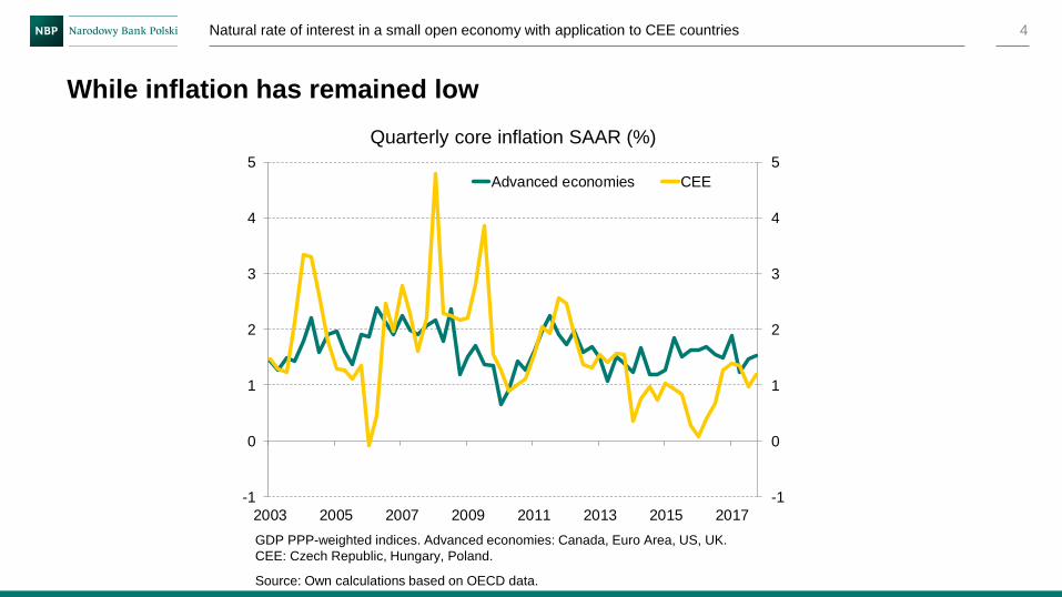
Quarterly core inflation SAAR (%)
GDP PPP-weighted indices. Advanced economies: Canada, Euro Area, US, UK.
CEE: Czech Republic, Hungary, Poland.
Source: Own calculations based on OECD data.
Natural rate of interest in a small open economy with application to CEE countries
While inflation has remained low
-1
0
1
2
3
4
5
-1
0
1
2
3
4
5
2003 2005 2007 2009 2011 2013 2015 2017
Advanced economies CEE
■ Inflation has become more dependent on external factors – oil prices, inflation and
output gap abroad (i.a. Auer et al., 2017)
■ Inflation expectations have fallen (Coibion and Gorodnichenko, 2015)
■ The links between interest rates, output and inflation have weakened – the Phillips
curve has flattened (i.a. Blanchard, 2016)
■ Natural interest rate has fallen significantly (Holston et al., 2017)
I investigate the latter and try to answer why it happened – if it happened
5
Potential explanations
Natural rate of interest in a small open economy with application to CEE countries

■ It is a real interest rate that would emerge under elastic prices and in the absence
of shocks. In such a case inflation is on target and output gap is zero (Woodford,
2003)
■ Several methods to estimate it:
■ Small structural model in the spirit of Laubach and Williams (2003): Holston et
al. (2017), Juselius et al. (2017), Kiley (2015), Pescatori and Turunen (2015)
■ DSGE model:
■ Short-term concept of NRI: Barsky et al. (2014), Curdia (2015), Del Negro et al. (2017)
■ Steady-state concept: German Council of Economic Experts (2015)
■ Medium-term concept: Del Negro et al. (2017)
■ VAR model: Lubik and Matthes (2015), Del Negro et al. (2017)
6
Natural rate of interest
Natural rate of interest in a small open economy with application to CEE countries

■ I use the framework from the latest study of Laubach and Williams (Holston et al., 2017) as a starting point:
■ Medium-term concept of NRI most relevant from policy perspective
■ Flexibility
■ However, it is a simple closed-economy framework not very suitable for small open economies like the CEE countries
■ Therefore, I use the open economy new Keynesian model of Gali and Monacelli (2005) as a base to derive the extended, open economy version of the Laubach-Williams framework
■ The model is augmented with i.a. the exchange rate, inflation expectations, energy prices, foreign output gap, lending spread and capacity utilisation
7
Estimation framework
Natural rate of interest in a small open economy with application to CEE countries

■ A system of equations estimated with Kalman filter:
■ Phillips curve:
𝜋𝑡 =
𝑖=1
4
𝑏𝜋,𝑖𝜋𝑡−𝑖 + 𝑏𝑦 𝑦𝑡 + 𝜖𝜋,𝑡
■ IS curve:
𝑦𝑡 = 𝑎𝑦,1 𝑦𝑡−1 + 𝑎𝑦,2 𝑦𝑡−2 +𝑎𝑟2
𝑗=1
2
(𝑟𝑡−𝑗 − 𝑟𝑡−𝑗∗ ) + 𝜖 𝑦,𝑡
■ Natural rate of interest:
𝑟𝑡∗ = 𝑔𝑡 + 𝑧𝑡
■ Remaining equations:
𝑦𝑡 = 𝑦𝑡∗ + 𝑦𝑡/100
𝑦𝑡∗ = 𝑦𝑡−1
∗ + 𝑔𝑡−1/400𝑔𝑡 = 𝑔𝑡−1 + 𝜖𝑔,𝑡𝑧𝑡 = 𝑧𝑡−1 + 𝜖𝑧,𝑡
8
Basic Holston-Laubach-Williams framework
Natural rate of interest in a small open economy with application to CEE countries

𝜋𝑡 - core inflation
𝑦𝑡 - ln GDP
𝑦𝑡∗ - ln potential GDP
𝑦𝑡 - output gap
𝑟𝑡 - real interest rate
𝑟𝑡∗ - natural interest rate
𝑔𝑡 - potential GDP growth
𝑧𝑡 - other determinants of natural interest rate
9
Variables description
Natural rate of interest in a small open economy with application to CEE countries
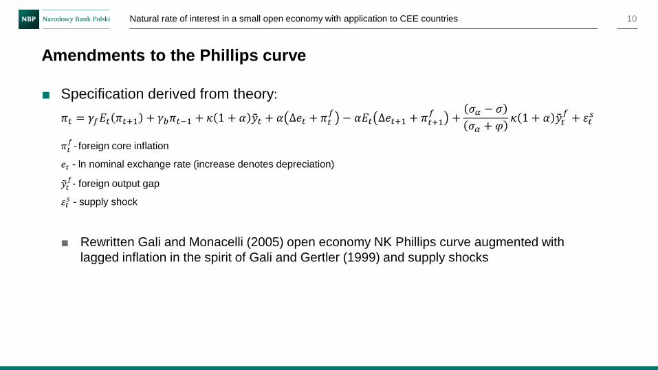
■ Specification derived from theory:
𝜋𝑡 = 𝛾𝑓𝐸𝑡 𝜋𝑡+1 + 𝛾𝑏𝜋𝑡−1 + 𝜅 1 + 𝛼 𝑦𝑡 + 𝛼 ∆𝑒𝑡 + 𝜋𝑡𝑓
− 𝛼𝐸𝑡 ∆𝑒𝑡+1 + 𝜋𝑡+1𝑓
+𝜎𝛼 − 𝜎
𝜎𝛼 + 𝜑𝜅 1 + 𝛼 𝑦𝑡
𝑓+ 휀𝑡
𝑠
𝜋𝑡𝑓- foreign core inflation
𝑒𝑡 - ln nominal exchange rate (increase denotes depreciation)
𝑦𝑡𝑓- foreign output gap
휀𝑡𝑠 - supply shock
■ Rewritten Gali and Monacelli (2005) open economy NK Phillips curve augmented with
lagged inflation in the spirit of Gali and Gertler (1999) and supply shocks
10
Amendments to the Phillips curve
Natural rate of interest in a small open economy with application to CEE countries
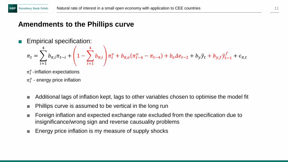
■ Empirical specification:
𝜋𝑡 =
𝑖=1
4
𝑏𝜋,𝑖𝜋𝑡−𝑖 + 1 −
𝑖=1
4
𝑏𝜋,𝑖 𝜋𝑡𝑒 + 𝑏𝜋,𝑜 𝜋𝑡−4
𝑜 − 𝜋𝑡−4 + 𝑏𝑒𝛥𝑒𝑡−2 + 𝑏𝑦 𝑦𝑡 + 𝑏𝑦,𝑓 𝑦𝑡−1𝑓
+ 𝜖𝜋,𝑡
𝜋𝑡𝑒- inflation expectations
𝜋𝑡𝑜 - energy price inflation
■ Additional lags of inflation kept, lags to other variables chosen to optimise the model fit
■ Phillips curve is assumed to be vertical in the long run
■ Foreign inflation and expected exchange rate excluded from the specification due to
insignificance/wrong sign and reverse causuality problems
■ Energy price inflation is my measure of supply shocks
11
Amendments to the Phillips curve
Natural rate of interest in a small open economy with application to CEE countries
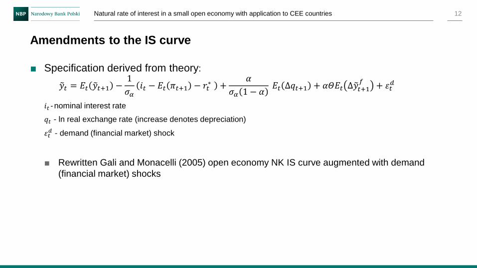
■ Specification derived from theory:
𝑦𝑡 = 𝐸𝑡 𝑦𝑡+1 −1
𝜎𝛼𝑖𝑡 − 𝐸𝑡 𝜋𝑡+1 − 𝑟𝑡
∗ +𝛼
𝜎𝛼 1 − 𝛼𝐸𝑡 ∆𝑞𝑡+1 + 𝛼𝛩𝐸𝑡 ∆ 𝑦𝑡+1
𝑓+ 휀𝑡
𝑑
𝑖𝑡- nominal interest rate
𝑞𝑡 - ln real exchange rate (increase denotes depreciation)
휀𝑡𝑑 - demand (financial market) shock
■ Rewritten Gali and Monacelli (2005) open economy NK IS curve augmented with demand
(financial market) shocks
12
Amendments to the IS curve
Natural rate of interest in a small open economy with application to CEE countries

■ Empirical specification:
𝑦𝑡 = 𝑎𝑦,1 𝑦𝑡−1 +𝑎𝑟2
𝑗=1
2
(𝑟𝑡−𝑗 − 𝑟𝑡−𝑗∗ ) + 𝑎𝑒𝛥𝑞𝑡−3 + 𝑎𝑓𝛥 𝑦𝑡
𝑓+ 𝑎𝑙𝑙𝑠𝑡 + 𝜖 𝑦,𝑡
𝑐𝑢𝑡 = 𝑦𝑡 + 𝜖𝑐𝑢,𝑡
𝑙𝑠𝑡- lending spread (deviation from mean)
𝑐𝑢𝑡- capacity utilisation
■ Only one lag to domestic output gap, two lags to real rate gap kept, lag to exchange rate
chosen to optimise the model fit
■ Lending spread (spread between market and central bank rates) is the measure of financial
market shocks – Kiley (2015) shows that accounting for it matters for NRI estimation
■ The use of survey data significantly improves the accuracy of output gap estimation
(Marcellino and Musso, 2011; ECB, 2015; Hulej and Grabek, 2015) and by making output
gap partially observable gives the model more power to estimate the NRI (𝑧𝑡 in particular)
13
Amendments to the IS curve
Natural rate of interest in a small open economy with application to CEE countries
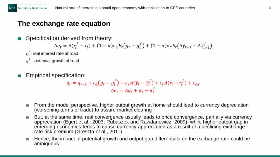
■ Specification derived from theory:
∆𝑞𝑡 = ∆(𝑟𝑡𝑓− 𝑟𝑡) + 1 − 𝛼 𝜎𝛼𝐸𝑡 𝑔𝑡 − 𝑔𝑡
𝑓+ 1 − 𝛼 𝜎𝛼𝐸𝑡 ∆ 𝑦𝑡+1 − ∆ 𝑦𝑡+1
𝑓
𝑟𝑡𝑓- real interest rate abroad
𝑔𝑡𝑓
- potential growth abroad
■ Empirical specification:
𝑞𝑡 = 𝑞𝑡−1 + 𝑐𝑔 𝑔𝑡 − 𝑔𝑡𝑓
+ 𝑐𝑦𝛥( 𝑦𝑡 − 𝑦𝑡𝑓) + 𝑐𝑟𝛥(𝑟𝑡 − 𝑟𝑡
𝑓) + 𝜖𝑒,𝑡
𝛥𝑒𝑡 = 𝛥𝑞𝑡 + 𝜋𝑡 − 𝜋𝑡𝑓
■ From the model perspective, higher output growth at home should lead to currency depreciation (worsening terms of trade) to assure market clearing
■ But, at the same time, real convergence usually leads to price convergence, partially via currency appreciation (Egert et al., 2003; Rubaszek and Rawdanowicz, 2009), while higher output gap in emerging economies tends to cause currency appreciation as a result of a declining exchange rate risk premium (Greszta et al., 2011)
■ Hence, the impact of potential growth and output gap differentials on the exchange rate could be ambiguous
14
The exchange rate equation
Natural rate of interest in a small open economy with application to CEE countries
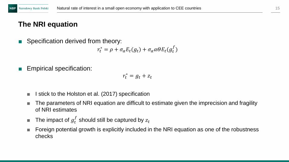
■ Specification derived from theory:
𝑟𝑡∗ = 𝜌 + 𝜎𝛼𝐸𝑡(𝑔𝑡) + 𝜎𝛼𝛼𝛩𝐸𝑡(𝑔𝑡
𝑓)
■ Empirical specification:𝑟𝑡∗ = 𝑔𝑡 + 𝑧𝑡
■ I stick to the Holston et al. (2017) specification
■ The parameters of NRI equation are difficult to estimate given the imprecision and fragility
of NRI estimates
■ The impact of 𝑔𝑡𝑓
should still be captured by 𝑧𝑡
■ Foreign potential growth is explicitly included in the NRI equation as one of the robustness
checks
15
The NRI equation
Natural rate of interest in a small open economy with application to CEE countries
■ Sample covers the euro area and 3 CEE economies: Poland, Czech Republic and
Hungary
■ Euro area is used as a proxy for the foreign sector of CEE (~60% of CEE foreign
trade is with the euro area) – euro area’s output gap, potential growth and real
interest rate used as 𝑦𝑡𝑓, 𝑔𝑡
𝑓and 𝑟𝑡
𝑓
■ US treated as a foreign sector for the euro area ( 𝑦𝑡𝑓
and 𝑔𝑡𝑓
calculated from the HP
filter)
■ Quarterly data, 1996Q2-2017Q4
16
Sample
Natural rate of interest in a small open economy with application to CEE countries

■ Inflation and real interest rate calculated similarly as in Holston et al. (2017):
■ Inflation: quarterly inflation excluding food and energy, seasonally adjusted and annualised,
from OECD
■ Real interest rate: central bank benchmark rate (from Bloomberg) minus annual core
inflation
■ Exceptions: for Hungary I use the 3-month interbank offer rate (similarly as in the euro area,
the benchmark interest rate changed there recently) and for the euro area the Wu-Xia
shadow rate is used so that unconventional policies are taken into account
■ Real interest rate deflated with inflation expectations used as a robustness check
17
Data
Natural rate of interest in a small open economy with application to CEE countries
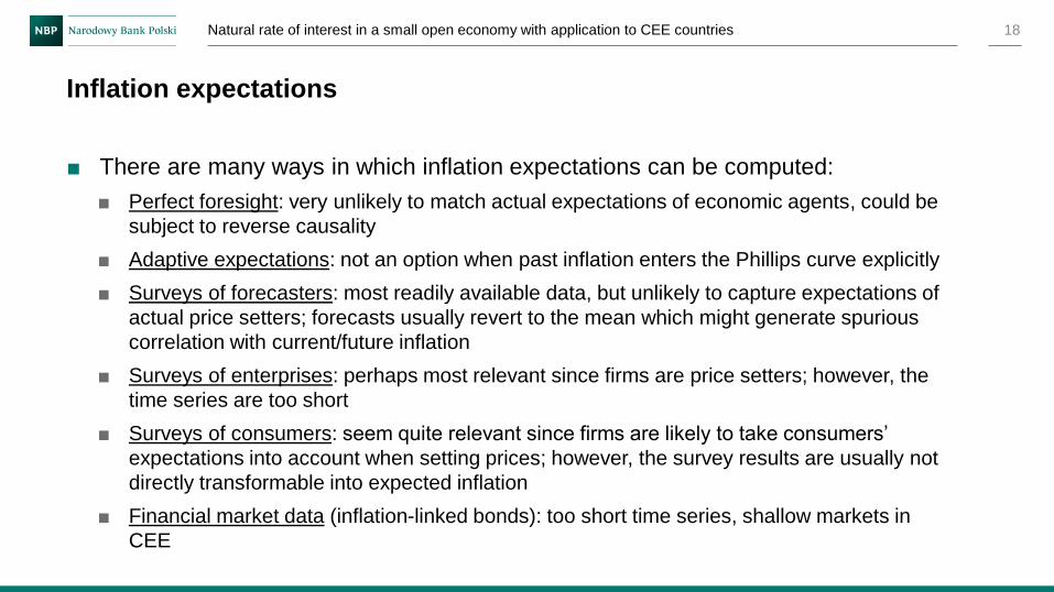
■ There are many ways in which inflation expectations can be computed:
■ Perfect foresight: very unlikely to match actual expectations of economic agents, could be
subject to reverse causality
■ Adaptive expectations: not an option when past inflation enters the Phillips curve explicitly
■ Surveys of forecasters: most readily available data, but unlikely to capture expectations of
actual price setters; forecasts usually revert to the mean which might generate spurious
correlation with current/future inflation
■ Surveys of enterprises: perhaps most relevant since firms are price setters; however, the
time series are too short
■ Surveys of consumers: seem quite relevant since firms are likely to take consumers’
expectations into account when setting prices; however, the survey results are usually not
directly transformable into expected inflation
■ Financial market data (inflation-linked bonds): too short time series, shallow markets in
CEE
18
Inflation expectations
Natural rate of interest in a small open economy with application to CEE countries

■ All things considered, I have opted to use consumer inflation expectations
■ Input data: expected price trends over the next 12 months from the European Commission
consumer survey, balance statistics
■ However, this data has to be transformed into expected inflation before it is incorporated
into my specification of the Phillips curve
■ Standard methods of balance statistic quantification result in expectations being closely
aligned with current inflation, to the extent they are no longer informative
■ Therefore, an alternative method is used - the balance statistic is simply rescaled such that:
■ mean = mean headline inflation
■ variance = 0.6 of headline inflation variance
■ The latter number comes from surveys where consumers are asked a quantitative question
(Czech Rep., US and UK; variance of expectations/variance of headline inflation = 0.54-
0.67)
19
Inflation expectations
Natural rate of interest in a small open economy with application to CEE countries

20
Inflation expectations
Natural rate of interest in a small open economy with application to CEE countries

■ In the literature, corporate bond spread is usually used as a measure of financial
market shocks (e.g. Kiley, 2015)
■ However, CEE economies are bank-dominated and corporate bond markets are
shallow
■ Therefore, an alternative measure (lending spread) is constructed:
■ Defined as a difference between mean interest rate on new bank loans and central bank
benchmark interest rate (the same as the one used to compute real interest rate)
■ Source: central bank interest rate statistics
■ Comparable and comprehensive data available since 2004, for the earlier period either
partial data from national sources (Poland, Hungary) or the data from IMF International
Statistics Database (euro area, Czechia) is used
■ The deviation of lending spread from the sample mean used in the estimation (for Hungary
the deviation from linear trend)
21
Lending spread
Natural rate of interest in a small open economy with application to CEE countries

22
Deviation of lending spread from the sample mean* (%)
* For Hungary, deviation from linear trend
Source: Own calculations based on central bank and IMF data.
Natural rate of interest in a small open economy with application to CEE countries
Lending spread
-8
-6
-4
-2
0
2
4
6
-8
-6
-4
-2
0
2
4
6
1996 1999 2002 2005 2008 2011 2014 2017
Euro Area Czechia Hungary* Poland

■ Capacity utilisation:
■ Actual capacity utilisation data is mostly unavailable for the service sector
■ Percentage of firms reporting insufficient demand as a factor limiting activity has been
proposed as a good alternative for the EU countries (ECB, 2015)
■ Data source: the European Commission business survey (for Poland GUS)
■ Weighted average for services, industry and construction; before 2003 the data for services
is not available and hence only industry and construction are included
■ Deviation from linear trend with an opposite sign is used in the estimation
■ Other data:
■ GDP: in constant prices and national currency, from OECD
■ Energy price inflation – QoQ, seasonally adjusted and annualised, from OECD
■ Real effective exchange rate (increase denotes appreciation) – from BIS
23
Other data
Natural rate of interest in a small open economy with application to CEE countries
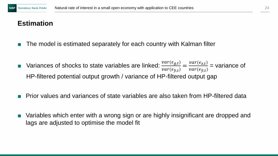
■ The model is estimated separately for each country with Kalman filter
■ Variances of shocks to state variables are linked: 𝑣𝑎𝑟(𝜖𝑔,𝑡)
𝑣𝑎𝑟(𝜖 𝑦,𝑡)=
𝑣𝑎𝑟(𝜖𝑧,𝑡)
𝑣𝑎𝑟(𝜖 𝑦,𝑡)= variance of
HP-filtered potential output growth / variance of HP-filtered output gap
■ Prior values and variances of state variables are also taken from HP-filtered data
■ Variables which enter with a wrong sign or are highly insignificant are dropped and
lags are adjusted to optimise the model fit
24
Estimation
Natural rate of interest in a small open economy with application to CEE countries
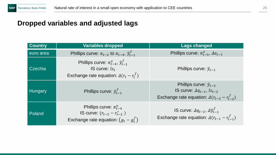
Country Variables dropped Lags changed
euro area Phillips curve: 𝜋𝑡−2 to 𝜋𝑡−4, 𝑦𝑡−1𝑓 Phillips curve: 𝜋𝑡−5
𝑜 , 𝛥𝑒𝑡−1
Czechia
Phillips curve: 𝜋𝑡−4𝑜 , 𝑦𝑡−1
𝑓
IS curve: 𝑙𝑠𝑡
Exchange rate equation: 𝛥(𝑟𝑡 − 𝑟𝑡𝑓)
Phillips curve: 𝑦𝑡−1
Hungary Phillips curve: 𝑦𝑡−1𝑓
Phillips curve: 𝑦𝑡−3IS curve: 𝛥𝑞𝑡−1, 𝑙𝑠𝑡−2
Exchange rate equation: 𝛥(𝑟𝑡−2 − 𝑟𝑡−2𝑓)
Poland
Phillips curve: 𝜋𝑡−4𝑜
IS curve: (𝑟𝑡−2 − 𝑟𝑡−2∗ )
Exchange rate equation: 𝑔𝑡 − 𝑔𝑡𝑓
IS curve: 𝛥𝑞𝑡−2, 𝛥 𝑦𝑡−1𝑓
Exchange rate equation: 𝛥(𝑟𝑡−1 − 𝑟𝑡−1𝑓)
25
Dropped variables and adjusted lags
Natural rate of interest in a small open economy with application to CEE countries
26Natural rate of interest in a small open economy with application to CEE countries
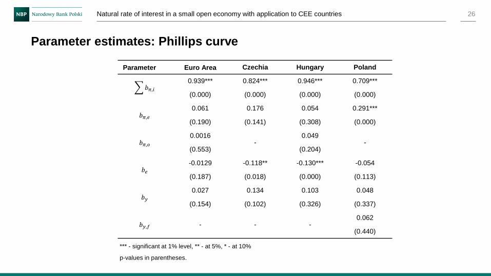
Parameter estimates: Phillips curve
Parameter Euro Area Czechia Hungary Poland
𝑏𝜋,𝑖0.939*** 0.824*** 0.946*** 0.709***
(0.000) (0.000) (0.000) (0.000)
𝑏𝜋,𝑒0.061 0.176 0.054 0.291***
(0.190) (0.141) (0.308) (0.000)
𝑏𝜋,𝑜0.0016
-0.049
-(0.553) (0.204)
𝑏𝑒-0.0129 -0.118** -0.130*** -0.054
(0.187) (0.018) (0.000) (0.113)
𝑏𝑦0.027 0.134 0.103 0.048
(0.154) (0.102) (0.326) (0.337)
𝑏𝑦,𝑓 - - -0.062
(0.440)
*** - significant at 1% level, ** - at 5%, * - at 10%
p-values in parentheses.

27Natural rate of interest in a small open economy with application to CEE countries
Parameter estimates: IS curve
Parameter Euro Area Czechia Hungary Poland
𝑎𝑦0.847*** 0.940*** 0.910*** 0.648***
(0.000) (0.000) (0.000) (0.000)
𝑎𝑟-0.205** -0.069* -0.068 -0.266***
(0.022) (0.061) (0.161) (0.000)
𝑎𝑒-0.040 -0.034 -0.063* -0.029
(0.181) (0.268) (0.080) (0.375)
𝑎𝑓0.412*** 0.687*** 0.681** 0.213
(0.000) (0.000) (0.014) (0.483)
𝑎𝑙-0.220*
--0.165 -0.425**
(0.098) (0.264) (0.016)
*** - significant at 1% level, ** - at 5%, * - at 10%
p-values in parentheses.
28Natural rate of interest in a small open economy with application to CEE countries
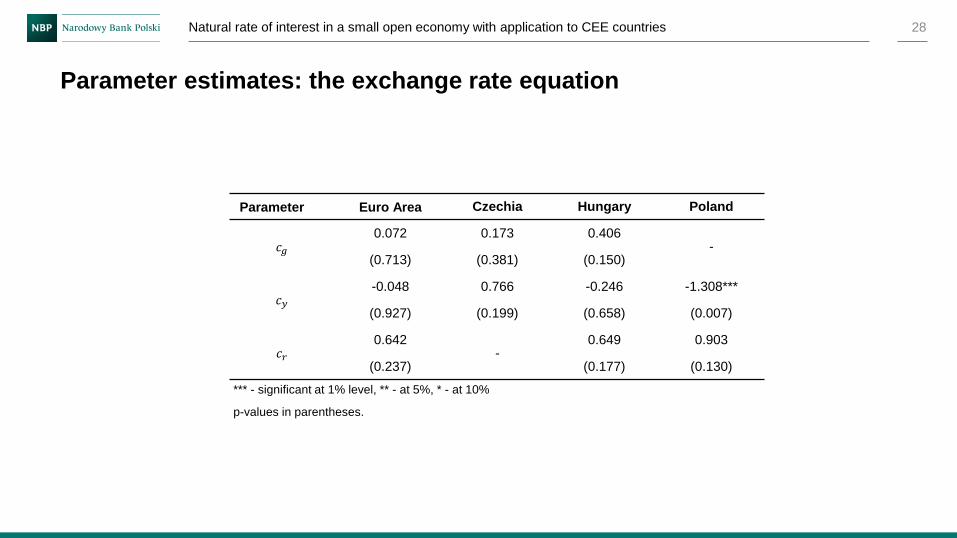
Parameter estimates: the exchange rate equation
Parameter Euro Area Czechia Hungary Poland
𝑐𝑔0.072 0.173 0.406
-(0.713) (0.381) (0.150)
𝑐𝑦-0.048 0.766 -0.246 -1.308***
(0.927) (0.199) (0.658) (0.007)
𝑐𝑟0.642
-0.649 0.903
(0.237) (0.177) (0.130)
*** - significant at 1% level, ** - at 5%, * - at 10%
p-values in parentheses.

29Natural rate of interest in a small open economy with application to CEE countries
Main results
-4
-2
0
2
4
6
8
-4
-2
0
2
4
6
8
1997 2000 2003 2006 2009 2012 2015
Euro Area Czechia Hungary Poland
■ NRI fell after the crisis but rebounded
in recent years
■ NRI is procyclical (correlation with
output gap 0.32-0.79)
■ NRI in Czechia and to some extent
Poland comoves with NRI in the euro
area
■ Hungary – suspicious case
Natural interest rate estimates (%)
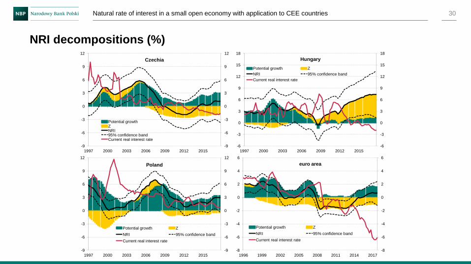
30Natural rate of interest in a small open economy with application to CEE countries
NRI decompositions (%)
-9
-6
-3
0
3
6
9
12
-9
-6
-3
0
3
6
9
12
1997 2000 2003 2006 2009 2012 2015
Czechia
Potential growthZNRI95% confidence bandCurrent real interest rate
-6
-3
0
3
6
9
12
15
18
-6
-3
0
3
6
9
12
15
18
1997 2000 2003 2006 2009 2012 2015
Hungary
Potential growth Z
NRI 95% confidence band
Current real interest rate
-9
-6
-3
0
3
6
9
12
-9
-6
-3
0
3
6
9
12
1997 2000 2003 2006 2009 2012 2015
Poland
Potential growth Z
NRI 95% confidence band
Current real interest rate
-8
-6
-4
-2
0
2
4
6
-8
-6
-4
-2
0
2
4
6
1996 1999 2002 2005 2008 2011 2014 2017
euro area
Potential growth Z
NRI 95% confidence band
Current real interest rate
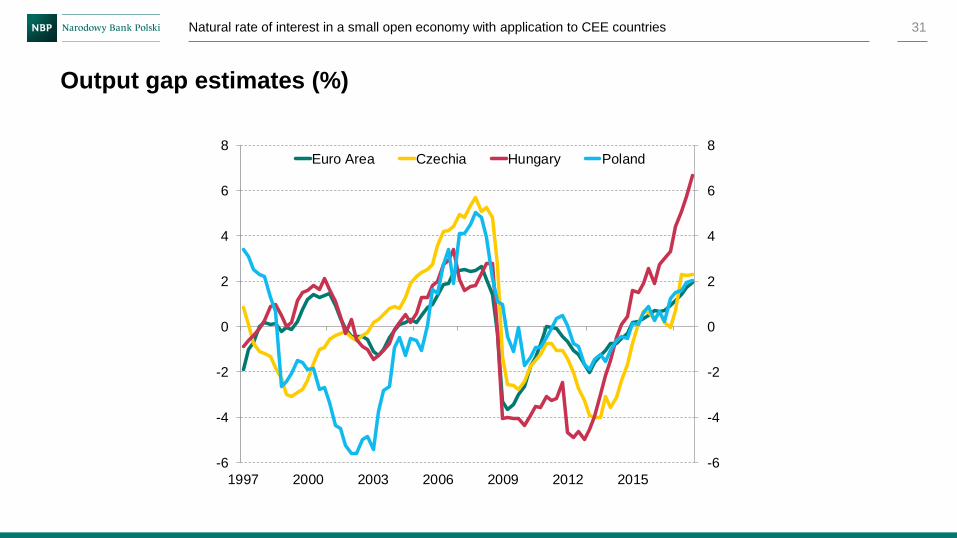
31Natural rate of interest in a small open economy with application to CEE countries
Output gap estimates (%)
-6
-4
-2
0
2
4
6
8
-6
-4
-2
0
2
4
6
8
1997 2000 2003 2006 2009 2012 2015
Euro Area Czechia Hungary Poland

32
Robustness checks: ex-ante real interest rate
Natural rate of interest in a small open economy with application to CEE countries
Natural interest rate estimates: baseline vs ex-ante real interest
rate (%)
Solid lines – baseline, dashed lines – ex-ante real interest rate
■ Interest rates deflated with consumer inflation
expectations instead of annual core inflation
■ Some differences in estimates, but for Czechia
and the euro area these stem from ex-ante
rates being consistently lower tan ex-post
rates, and for Poland from smaller sample size
■ After correcting for these effects, mean
absolute deviation <0.4 pp
■ Overall model performance virtually unchanged
■ Hungary – results not reported as the IS curve
relationship breaks up
-4
-2
0
2
4
6
8
-4
-2
0
2
4
6
8
1997 2000 2003 2006 2009 2012 2015
Euro Area Czechia Poland
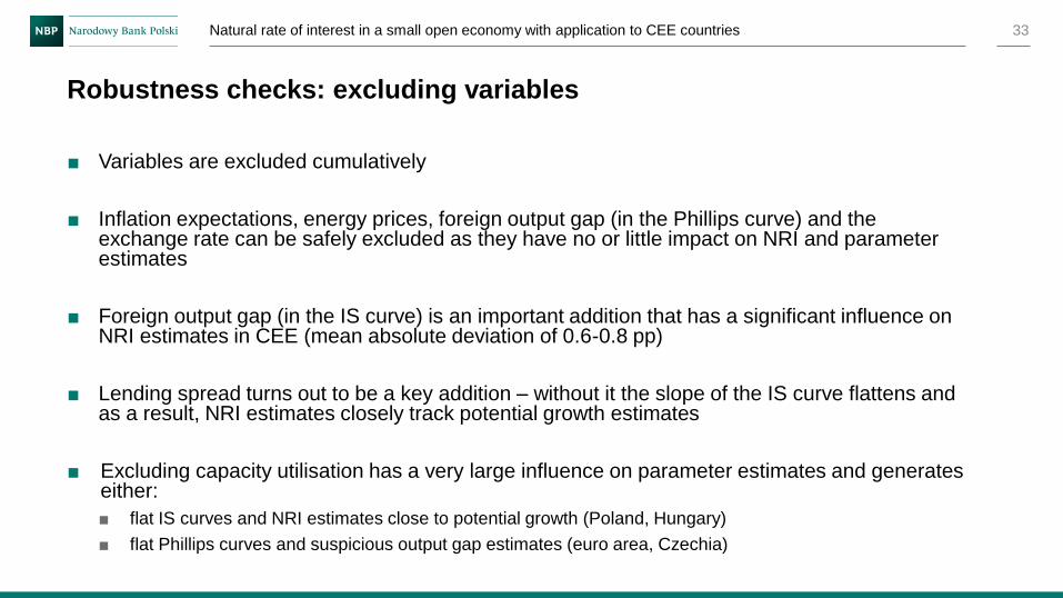
■ Variables are excluded cumulatively
■ Inflation expectations, energy prices, foreign output gap (in the Phillips curve) and the exchange rate can be safely excluded as they have no or little impact on NRI and parameter estimates
■ Foreign output gap (in the IS curve) is an important addition that has a significant influence on NRI estimates in CEE (mean absolute deviation of 0.6-0.8 pp)
■ Lending spread turns out to be a key addition – without it the slope of the IS curve flattens and as a result, NRI estimates closely track potential growth estimates
■ Excluding capacity utilisation has a very large influence on parameter estimates and generates either:
■ flat IS curves and NRI estimates close to potential growth (Poland, Hungary)
■ flat Phillips curves and suspicious output gap estimates (euro area, Czechia)
33
Robustness checks: excluding variables
Natural rate of interest in a small open economy with application to CEE countries

34Natural rate of interest in a small open economy with application to CEE countries
Robustness checks: excluding variables
-4
-2
0
2
4
6
8
-4
-2
0
2
4
6
8
1997 2000 2003 2006 2009 2012 2015
Czechia
Baseline
Simplified Phillips curve
No exchange rate block
No foreign output gap
No capacity utilisation (Laubach-Williams)-6
-4
-2
0
2
4
6
8
-6
-4
-2
0
2
4
6
8
1997 2000 2003 2006 2009 2012 2015
Hungary
Baseline
Simplified Phillips curve
No exchange rate block
No foreign output gap
No lending spread
No capacity utilisation (Laubach-Williams)
-4
-2
0
2
4
6
8
10
-4
-2
0
2
4
6
8
10
1997 2000 2003 2006 2009 2012 2015
Poland
BaselineSimplified Phillips curveNo exchange rate blockNo foreign output gapNo lending spreadNo capacity utilisation (Laubach-Williams)
-4
-2
0
2
4
-4
-2
0
2
4
1996 1999 2002 2005 2008 2011 2014 2017
euro area
Baseline
Simplified Phillips curve
No exchange rate block
No foreign output gap
No lending spread
No capacity utilisation (Laubach-Williams)
In the simplified specifications, variables are excluded cumulatively e.g. the “no exchange rate block” specification excludes the same variables as the “simplified Phillips curve” specification, plus the exchange rate variables.
Simplified Phillips curve: no energy prices, foreign output gap and inflation expectations in the Phillips curve; No exchange rate block: no exchange rate in Phillips and IS curves and no exchange rate equation; No foreign output gap: no foreign output gap in the IS curve; No lending spread: no lending spread in the IS curve; No capacity utilisation: no capacity utilisation equation.

35
Robustness checks: excluding variables
Natural rate of interest in a small open economy with application to CEE countries
Mean NRI standard errors (pp)■ The latter specification is largely
equivalent to the Holston et al. (2017)
specification
■ The accuracy of my estimates is 2-4
times larger
Specification Euro Area Czechia Hungary Poland
Baseline 0.58 1.59 2.04 1.05
Simplified Phillips
curve0.58 1.64 2.05 1.04
No exchange rate
block0.56 1.70 2.05 1.06
No foreign output
gap0.49 2.57 1.73 1.09
No lending spread 0.71 - 1.86 4.85
Laubach-Williams 1.91 3.02 3.88 4.15
36
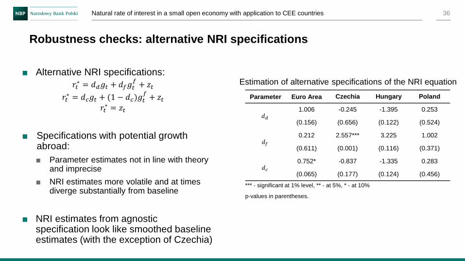
Robustness checks: alternative NRI specifications
Natural rate of interest in a small open economy with application to CEE countries
Estimation of alternative specifications of the NRI equation■ Alternative NRI specifications:
𝑟𝑡∗ = 𝑑𝑑𝑔𝑡 + 𝑑𝑓𝑔𝑡
𝑓+ 𝑧𝑡
𝑟𝑡∗ = 𝑑𝑐𝑔𝑡 + (1 − 𝑑𝑐)𝑔𝑡
𝑓+ 𝑧𝑡
𝑟𝑡∗ = 𝑧𝑡
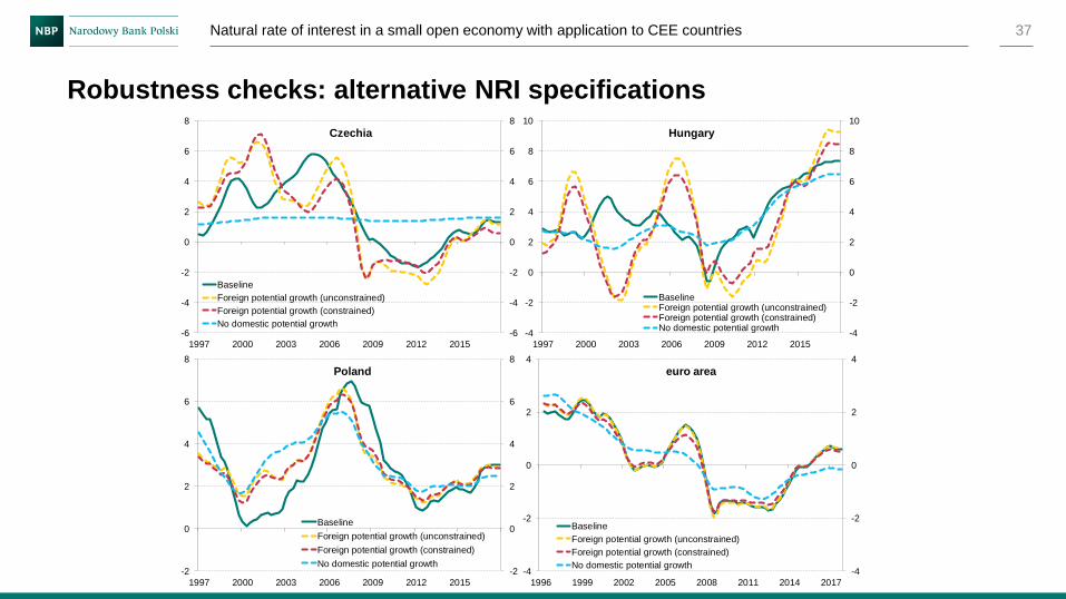
■ Specifications with potential growthabroad:
■ Parameter estimates not in line with theory and imprecise
■ NRI estimates more volatile and at times diverge substantially from baseline
■ NRI estimates from agnostic specification look like smoothed baseline estimates (with the exception of Czechia)
Parameter Euro Area Czechia Hungary Poland
𝑑𝑑1.006 -0.245 -1.395 0.253
(0.156) (0.656) (0.122) (0.524)
𝑑𝑓0.212 2.557*** 3.225 1.002
(0.611) (0.001) (0.116) (0.371)
𝑑𝑐0.752* -0.837 -1.335 0.283
(0.065) (0.177) (0.124) (0.456)
*** - significant at 1% level, ** - at 5%, * - at 10%
p-values in parentheses.
37Natural rate of interest in a small open economy with application to CEE countries
Robustness checks: alternative NRI specifications
-4
-2
0
2
4
6
8
10
-4
-2
0
2
4
6
8
10
1997 2000 2003 2006 2009 2012 2015
Hungary
BaselineForeign potential growth (unconstrained)Foreign potential growth (constrained)No domestic potential growth
-2
0
2
4
6
8
-2
0
2
4
6
8
1997 2000 2003 2006 2009 2012 2015
Poland
Baseline
Foreign potential growth (unconstrained)
Foreign potential growth (constrained)
No domestic potential growth-4
-2
0
2
4
-4
-2
0
2
4
1996 1999 2002 2005 2008 2011 2014 2017
euro area
Baseline
Foreign potential growth (unconstrained)
Foreign potential growth (constrained)
No domestic potential growth
-6
-4
-2
0
2
4
6
8
-6
-4
-2
0
2
4
6
8
1997 2000 2003 2006 2009 2012 2015
Czechia
Baseline
Foreign potential growth (unconstrained)
Foreign potential growth (constrained)
No domestic potential growth
38
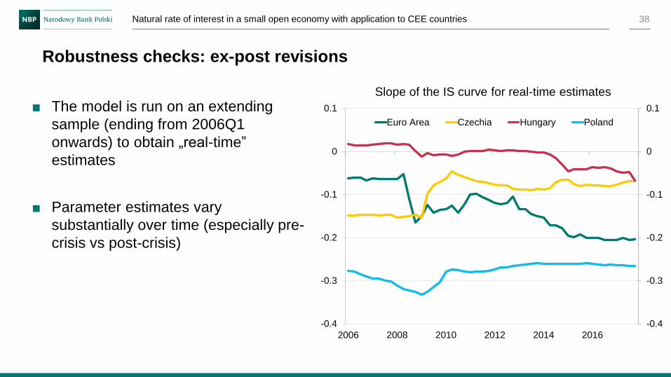
Robustness checks: ex-post revisions
Natural rate of interest in a small open economy with application to CEE countries
Slope of the IS curve for real-time estimates
■ The model is run on an extending
sample (ending from 2006Q1
onwards) to obtain „real-time”
estimates
■ Parameter estimates vary
substantially over time (especially pre-
crisis vs post-crisis)
-0.4
-0.3
-0.2
-0.1
0
0.1
-0.4
-0.3
-0.2
-0.1
0
0.1
2006 2008 2010 2012 2014 2016
Euro Area Czechia Hungary Poland

39
Robustness checks: ex-post revisions
Natural rate of interest in a small open economy with application to CEE countries
NRI estimates: baseline vs real-time estimates (%)
Solid lines – baseline, dashed lines – real-time estimates
■ Varying parameter estimates, together
with differences in input data
(detrended survey data), generate
significant ex-post revisions in NRI
estimates (0.9-2.3 pp on average),
especially around GFC and the euro
area crisis
■ For Hungary, real-time estimates are
consistently below baseline,
underlining the fragility of its results
-4
-2
0
2
4
6
8
10
12
-4
-2
0
2
4
6
8
10
12
2006 2008 2010 2012 2014 2016
Euro Area Czechia Hungary Poland

40Natural rate of interest in a small open economy with application to CEE countries
NRI lower than in the pre-crisis peak
The fall in natural interest rate since the crisis (percentage points)*
* 2005Q1 for Hungary and Czechia, 2007Q3 for Poland and 2006Q3 for the euro area.
-6
-4
-2
0
2
4
6
Czechia Hungary Poland euro area
Potential growth (g) Other determinants (z)

41Natural rate of interest in a small open economy with application to CEE countries
Potential drivers of falling natural interest rates
Internal External
Potential growth
• Decline in steady state
output level
• Slowdown in population
growth
• Slower rise in labour
participation
• Convergence
• Slowdown in global TFP
growth
Other determinants
• Population ageing
• Rising inequality
• Declining relative price
of capital
• Shifts in preferences
(“saving glut”)
• Population ageing
abroad
• Rising inequality abroad
• Declining relative price
of capital abroad
• Shifts in preferences
abroad
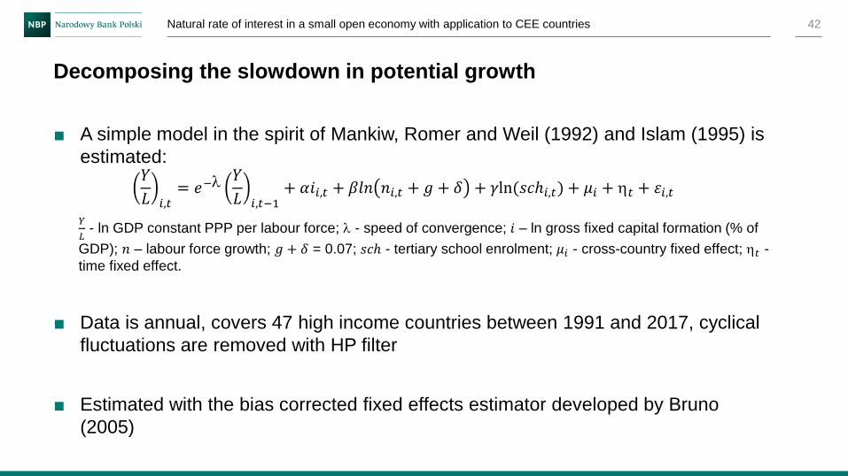
■ A simple model in the spirit of Mankiw, Romer and Weil (1992) and Islam (1995) is
estimated: 𝑌
𝐿 𝑖,𝑡= 𝑒−
𝑌
𝐿 𝑖,𝑡−1+ 𝛼𝑖𝑖,𝑡 + 𝛽𝑙𝑛 𝑛𝑖,𝑡 + 𝑔 + 𝛿 + 𝛾ln(𝑠𝑐ℎ𝑖,𝑡) + 𝜇𝑖 + 𝑡 + 휀𝑖,𝑡
𝑌
𝐿- ln GDP constant PPP per labour force; - speed of convergence; 𝑖 – ln gross fixed capital formation (% of
GDP); 𝑛 – labour force growth; 𝑔 + 𝛿 = 0.07; 𝑠𝑐ℎ - tertiary school enrolment; 𝜇𝑖 - cross-country fixed effect; 𝑡 -
time fixed effect.
■ Data is annual, covers 47 high income countries between 1991 and 2017, cyclical
fluctuations are removed with HP filter
■ Estimated with the bias corrected fixed effects estimator developed by Bruno
(2005)
42
Decomposing the slowdown in potential growth
Natural rate of interest in a small open economy with application to CEE countries

■ Using estimated model parameters, potential growth can be decomposed:
𝑔𝑡 = 𝑔𝑡𝐴 + λ
𝑌
𝐿 𝑝𝑒𝑎𝑘
𝑠𝑠
−𝑌
𝐿 𝑡+ λ
𝑌
𝐿 𝑡
𝑠𝑠
−𝑌
𝐿 𝑝𝑒𝑎𝑘
𝑠𝑠
+ 𝑛𝑡𝑝𝑜𝑝
+ 𝑛𝑡 − 𝑛𝑡𝑝𝑜𝑝
+ 휀𝑖,𝑡
𝑔𝑡𝐴 = 𝑡 − 1 − 𝑒− 𝑡 − 1
𝑡
𝑡−𝑒− 𝑡−1: global TFP growth
𝑛𝑡𝑝𝑜𝑝
: working age population growth
λ𝑌
𝐿 𝑝𝑒𝑎𝑘
𝑠𝑠−
𝑌
𝐿 𝑡= 𝑒−
𝑌
𝐿 𝑖,𝑡−1+ 𝛼𝑖𝑖,𝑝𝑒𝑎𝑘 + 𝛽𝑙𝑛 𝑛𝑖,𝑝𝑒𝑎𝑘 + 𝑔 + 𝛿 + 𝛾ln(𝑠𝑐ℎ𝑖,𝑝𝑒𝑎𝑘) + 𝜇𝑖 −
𝑌
𝐿 𝑖,𝑡−1+
1 − 𝑒− 𝑡 − 1𝑡
𝑡−𝑒− 𝑡−1: convergence
λ𝑌
𝐿 𝑡
𝑠𝑠−
𝑌
𝐿 𝑝𝑒𝑎𝑘
𝑠𝑠= 𝛼(𝑖𝑖,𝑡−𝑖𝑖,𝑝𝑒𝑎𝑘) + 𝛽(ln 𝑛𝑖,𝑡 − ln𝑛𝑖,𝑝𝑒𝑎𝑘) + 𝛾(ln 𝑠𝑐ℎ𝑖,𝑡 − ln 𝑠𝑐ℎ𝑖,𝑝𝑒𝑎𝑘): steady state
movements
peak is the year of pre-crisis peak: 2005 for Czechia and Hungary, 2006 for the euro area and 2007 for Poland
43
Decomposing the slowdown in potential growth
Natural rate of interest in a small open economy with application to CEE countries

44Natural rate of interest in a small open economy with application to CEE countries
Growth model estimation results
Variable Coefficient
L.𝑌
𝐿
0.9838
(0.000)
𝑖0.0514
(0.000)
𝑙𝑛 𝑛𝑖,𝑡 + 𝑔 + 𝛿-0.0437
(0.000)
ln(𝑠𝑐ℎ𝑖,𝑡)0.0104
(0.000)
No. of observations 1018
No. of countries 47
R2 0.999
p-values in parentheses.

45
Domestic factors more important than global factors
Natural rate of interest in a small open economy with application to CEE countries
Potential growth slowdown vs the pre-crisis peak (pp)
Pre-crisis peak in 2005 for Czechia and Hungary, 2006 for the euro area and 2007 for Poland.
The growth slowdown stemming from convergence calculated assuming steady state determinants
remain constant at the pre-crisis level.
Dark grey bars show the discrepancy between potential growth rates obtained from the HP filter and
the ones estimated from the Kalman filter.
■ Convergence, a fall in investment/GDP ratio and the slowdown in global TFP growth all played role in CEE growth slowdown
■ In Hungary, higher labour force growth and falling school enrolment had an additional negative effect on steady state
■ Shrinking working age population was mostly offset by increasing labour participation
■ In the euro area, global factors and slower labour force growth most important
-2
-1
0
1
2
3
4
5
6
-2
-1
0
1
2
3
4
5
6
Czechia Hungary Poland Euro Area
Discrepancy in potential growth rates Model residualLabour force participation Population growthTechnology Steady stateConvergence Overall slowdown

■ Other drivers of NRI:
■ For a panel of CEE countries, 𝑧𝑡 regressed on old-age dependency ratio, Gini
coefficient, relative price of capital, saving-investment gap and 𝑧𝑡 in the euro
area
46
What’s next?
Natural rate of interest in a small open economy with application to CEE countries
■ Adding capacity utilisation, lending spread and foreign output gap improves the performance of Holston-Laubach-Williams model and makes it more suitable to study small open economies such as CEE
■ The model has more power to estimate 𝑧𝑡
■ Ex-ante errors decrease substantially
■ NRI fell after the crisis and rebounded in recent years, but remains lower than in the pre-crisis peak (in Poland and Czechia by 4-5 pp)
■ Both 𝑔𝑡 and 𝑧𝑡 play a significant role in NRI developments
■ Domestic factors (convergence and falling investment/GDP ratio) contributed more to potential growth slowdown than global factors
47
Conclusions
Natural rate of interest in a small open economy with application to CEE countries

48
Policy implications
Natural rate of interest in a small open economy with application to CEE countries
Real interest rates in Poland: actual vs Taylor rules (%)
Taylor rule specification: 𝑟𝑡 = 𝑟𝑡∗ + 0.5 𝑦𝑡 + 0.5(𝜋𝑡 − 𝜋𝑡), where 𝜋𝑡 is inflation target.
Constant NRI = NRI sample mean.
■ NRI procyclical monetary policy
should react to cyclical fluctuations
more strongly
■ Current stance too loose (in Czechia,
Hungary and the euro area way more
than in Poland)
-4
-2
0
2
4
6
8
10
12
-4
-2
0
2
4
6
8
10
12
1998 2001 2004 2007 2010 2013 2016
Actual real interest rate
Taylor rule
Taylor rule with constant NRI

■ Heavy dependence on survey data low quality of survey data one of the
reasons why NRI estimates for Hungary are doubtful
■ Specification of the NRI equation is a soft spot: domestic growth does not seem to
be the main driver of NRI in reality (fully agnostic specification better?)
■ Parameter estimates are vulnerable to sample choice, which results in large ex-
post revisions of NRI estimates
■ Growth model is simplistic; in particular, it does not control (well) for cross-country
differences in TFP growth
49
Caveats
Natural rate of interest in a small open economy with application to CEE countries
■ Auer, R. A., Borio, C. E., & Filardo, A. J. (2017). The globalisation of inflation: the growing importance of global value
chains. CESifo Working Paper, 6387.
■ Barsky, R., Justiniano, A., & Melosi, L. (2014). The natural rate of interest and its usefulness for monetary policy.
American Economic Review, 104(5), 37-43.
■ Blanchard, O. (2016). The Phillips Curve: Back to the'60s?. American Economic Review, 106(5), 31-34.
■ Bruno, G. S. (2005). Approximating the bias of the LSDV estimator for dynamic unbalanced panel data models.
Economics letters, 87(3), 361-366.
■ Carlson, J. A., & Parkin, M. (1975). Inflation expectations. Economica, 42(166), 123-138.
■ Clarida, R., Gali, J., & Gertler, M. (1999). The science of monetary policy: a new Keynesian perspective. Journal of
economic literature, 37(4), 1661-1707.
■ Coibion, O., & Gorodnichenko, Y. (2015). Is the Phillips curve alive and well after all? Inflation expectations and the
missing disinflation. American Economic Journal: Macroeconomics, 7(1), 197-232.
■ Cúrdia, V. (2015). Why so slow? A gradual return for interest rates. Federal Reserve Bank of San Francisco Economic
Letter, 32.
■ Del Negro, M., Giannone, D., Giannoni, M. P., & Tambalotti, A. (2017). Safety, liquidity, and the natural rate of interest.
Brookings Papers on Economic Activity, 2017(1), 235-316.
■ Égert, B., Drine, I., Lommatzsch, K., & Rault, C. (2003). The Balassa–Samuelson effect in Central and Eastern Europe:
myth or reality?. Journal of comparative Economics, 31(3), 552-572.
50
Literature
Natural rate of interest in a small open economy with application to CEE countries

■ European Central Bank (2015). A survey-based measure of slack for the euro area. ECB Economic Bulletin, 6/2015, Box
6.
■ Gali, J., & Gertler, M. (1999). Inflation dynamics: A structural econometric analysis. Journal of monetary Economics, 44(2),
195-222.
■ Gali, J., & Monacelli, T. (2005). Monetary policy and exchange rate volatility in a small open economy. The Review of
Economic Studies, 72(3), 707-734.
■ German Council of Economic Experts (2015). Focus on Future Viability. Annual Economic Report.
■ Greszta, M., Hulej, M., Krzesicki, O., Lewińska, R., Pońsko, P., Rybaczyk, B., & Tarnicka, M. (2011). Reestymacja
kwartalnego modelu gospodarki polskiej NECMOD 2011.
■ Hulej, M., & Grabek, G. (2015). Output gap measure based on survey data. NBP Working Paper, 200.
■ Holston, K., Laubach, T., & Williams, J. C. (2017). Measuring the natural rate of interest: International trends and
determinants. Journal of International Economics, 108, S59-S75.
■ Islam, N. (1995). Growth empirics: a panel data approach. The Quarterly Journal of Economics, 110(4), 1127-1170.
■ Juselius, M., Borio, C., Disyatat, P., & Drehmann, M. (2017). Monetary Policy, the Financial Cycle, and Ultra-Low Interest
Rates. International Journal of Central Banking.
■ Kiley, M. T. (2015). What can the data tell us about the equilibrium real interest rate?. Finance and Economics Discussion
Series, 2015-077.
51
Literature
Natural rate of interest in a small open economy with application to CEE countries

■ Laubach, T., & Williams, J. C. (2003). Measuring the natural rate of interest. Review of Economics and Statistics, 85(4),
1063-1070.
■ Lubik, T. A., & Matthes, C. (2015). Calculating the natural rate of interest: A comparison of two alternative approaches.
Richmond Fed Economic Brief, (Oct), 1-6.
■ Mankiw, N. G., Romer, D., & Weil, D. N. (1992). A contribution to the empirics of economic growth. The quarterly journal of
economics, 107(2), 407-437.
■ Marcellino, M., & Musso, A. (2011). The reliability of real-time estimates of the euro area output gap. Economic Modelling,
28(4), 1842-1856.
■ Pescatori, A., & Turunen, M. J. (2015). Lower for longer: Neutral rates in the united states. IMF Working Paper, 15-135.
■ Rubaszek, M., & Rawdanowicz, Ł. (2009). Economic convergence and the fundamental equilibrium exchange rate in
central and eastern Europe. International Review of Financial Analysis, 18(5), 277-284.
■ Solow, R. M. (1956). A contribution to the theory of economic growth. The quarterly journal of economics, 70(1), 65-94.
■ Taylor, J. B. (1993). Discretion versus policy rules in practice. Carnegie-Rochester conference series on public policy, 39,
195-214.
■ Woodford, M. (2003). Interest and Prices: Foundations of a Theory of Monetary Policy. Princeton University Press.
■ Wu, J. C., & Xia, F. D. (2017). Time-varying lower bound of interest rates in Europe.
52
Literature
Natural rate of interest in a small open economy with application to CEE countries
