natural gas activities air monitoring initiative … objectives ..... 12 project design..... 13 site...
TRANSCRIPT

EPA Region III
Natural Gas Ambient Air
Monitoring Initiative (NGAAMI) in
Southwestern Pennsylvania
Air Protection Division,
Office of Air Monitoring and Analysis
August 2015

Page 2
Table of Contents
Acknowledgments ............................................................................................................. 5
Executive Summary ......................................................................................................... 6
Natural Gas Ambient Air Monitoring Initiative (NGAAMI) .............................................. 8
Introduction ............................................................................................................................................ 8
Methods and materials ................................................................................................... 11
Specific Aims .......................................................................................................................................... 11
Project Objectives ........................................................................................................... 12
Project Design ................................................................................................................. 13
Site Selection .......................................................................................................................................... 13
VOC Canister Sampling and Analysis................................................................................................. 14
PM2.5 Sampling and Analysis .............................................................................................................. 15
Meteorological Monitoring ................................................................................................................. 15
Sampling Schedule ......................................................................................................... 15
Privacy and participation consent ................................................................................... 16
Informed Consent Procedures ............................................................................................................... 17
Description of Geographic Area ............................................................................................................. 17
Demographics ..................................................................................................................................... 17
Data Structure ................................................................................................................ 17
Lab Results ............................................................................................................................................. 17
Meteorological Data ............................................................................................................................... 18
Health and Safety Threshold Values ...................................................................................................... 21
Statistical Methods used and Data Analyses Conducted ................................................. 24
Location 2 and Collocated Location 2 ............................................................................................... 27
Descriptive Statistics ..................................................................................................... 28
Comparison Values ......................................................................................................... 32
Results and Interpreation ............................................................................................... 32
PM 2.5 ................................................................................................................................................... 32

Page 3
Comparison Values: Hazardous Air Pollutants .................................................................................... 34
Conclusion ...................................................................................................................... 35
References ..................................................................................................................... 36
List of Figures
Figure 1: Depth of Marcellus Shale Base ........................................................................................ 9
Figure 2: State of Pennsylvania and Washington County .............................................................10
Figure 3: Google Earth View of the Brigich Compressor Station, Chartiers Township, PA .......... 14
Figure 4 Distribution Counts by Frequency of Compounds .......................................................... 14
Figure 5 Wind Rose October 22, 2013 from PADEP onsite Weather Station .............................. 20
List of Tables
Table 1 EPA Region 3 Volatile Organic Compounds Valid Sampling Days ................................... 16 Table 2 Cancer-based and Non-cancer based Long Term Comparison Values * ......................... 22 Table 3: Data Sets Used in the Data Cleaning and Validation Process ........................................ 26 Table 4: Description of Lab Qualifiers 1. ...................................................................................... 26 Table 5: Frequency Counts of the Top eight Compounds ............................................................ 30 Table 6: Anaylsis of Variance for the eight most Frequent Compounds ...................................... 30 Table 7: Summary of Results (24-hr standard = 35 ug/m3) ........................................................ 33
Abbreviations and Acronyms
NGAAMI Natural Gas Ambient Air Monitoring Initiative VOCs Volatile Organic Compounds PM2.5 Particulate Matter less the 2.5 microns aerodynamic diameter ATSDR Agency for Toxic Substance and Disease Registry NAAQS National Ambient Air Quality Standards PADEP Pennsylvania Department of Environmental Protection APD Environmental Protection Agency Region III’s Air Protection Division SWPA Southwest Pennsylvania QA Quality Assurance CFR Code of Federal Regulations OASQA Office of Analytical Services and Quality Assurance MDL Minimum Detection Limits ppbv parts-per-billion-volume ug/m3 micrograms per cubic meter PTFE polytetrafluoroethylene FRM Federal Reference Method FEM Federal Equivalent Method QAPP Quality Assurance Project Plan NWS National Weather Service PIT Pittsburgh International Airport
Page 4
OAQPS Office of Air Quality Planning and Standards TCEQ Texas Commission on Environmental Quality’s CREG ATSDR’s Cancer Risk Evaluation Guides ANOVA Analysis of Variance
Appendix A: Data tables and Statistical Output
Appendix B: Additional Statistical Longitudinal Data Analysis for Volatile Organic Compounds
Appendix C: Raw Data Provided by Laboratory
Appendix D: TO 15 Compounds with LAB Method Detection Limits (MDL) and LAB Reporting Limits (RL)
Appendix E: Quality Assurance Project Plan, EPA Region 3, Natural Gas Activities Air Monitoring Initiative (NGAAMI): Revision No. 2.5, June, 2012
Page 5
Acknowledgments
This work would not have been possible without the assistance of many people from the Environmental
Protection Agency Region III (EPA) Office as well as the EPA Laboratory in Fort Meade and
collaboration with the Agency for Toxics Disease Registry. We also wish to thank the Pennsylvania
Department of Environmental Protection (PADEP) for their assistance and cooperation with providing
EPA site specific weather data for this effort. In addition, graduate student, Allison Jervis, MPH, for her
assistance in the Longitudinal Data Analysis for Volatile Organic Compounds analysis used for the
completion of her Master in Public Health at Drexel University. And finally this effort would not have
been possible without participation of the residents in Washington County that allowed EPA to collect
this data.
Authors: Carol Ann Gross-Davis, PhD, MS, Howard Schmidt, MS, MBA, Kia Hence, and Loretta Hyden,
EPA Region 3, Air Protection Division

Page 6
This document describes the analysis of air monitoring and other data collected from a late
summer though fall of 2012 under EPA’s initiative Natural Gas Ambient Air Monitoring
Initiative (NGAAMI) to assess potentially elevated levels of air toxics and PM2.5 concentrations
around natural gas extraction facilities. The document has been prepared for technical
audiences (e.g., risk assessors, meteorologists) and their management. It is intended to
describe the technical analysis of data collected for this in clear, but generally technical, terms.
Executive Summary
Air monitoring has been conducted at three residential properties around the Brigich
Compressor Station in Washington County, Pennsylvania as part of the EPA Region
3 initiative to monitor specific air toxic compounds in the outdoor air around natural
gas extraction facilities.
The Brigich location was selected for monitoring based on residential homes in close
proximity (<0.5 miles) to the facility, the premise that the facility was in operation
“long-term” more than five years, topography and availability of monitoring site
access.
Air monitoring was performed from (August 4, 2012 to November 25, 2012) for the
following pollutants: Volatile Organic Compounds (VOCs) also commonly referred
to as Hazardous Air Pollutants (HAPs) & Particulate Matter less the 2.5 microns
aerodynamic diameter (PM2.5)
Measured levels of VOCs (i.e. 1,3-butadiene and benzene) were compared to
associated longer-term concentration estimates to determine if concentrations
exceeded the long-term and/or short term risk levels calculated by EPA and Agency
for Toxic Substance and Disease Registry (ATSDR).
Results from the VOC monitoring did not indicate any level of concern.

Page 7
PM2.5 data was compared to the 24 hour National Ambient Air Quality Standards
(NAAQS) because there was not enough sample days during the initiative to compare
to the Annual NAAQS.
Results from PM2.5 data did not indicate any level of concern.
Based on the sampling results from the (NGAAMI), EPA Region 3 recommends that
no additional VOC and PM2.5 monitoring is necessary at the sampling locations
around the Brigich Compressor Station. However, EPA’s ongoing research and
national air toxics monitoring programs will continue to collect information on
natural gas source impacts on outdoor air.

Page 8
Natural Gas Ambient Air Monitoring Initiative (NGAAMI)
Introduction
Pennsylvania has seen rapid development of the Marcellus Shale industry since 2007. The
Pennsylvania Department of Environmental Protection (PADEP) has primary environmental
regulatory authority over this booming industry. Since drilling began, the PADEP has
implemented voluntary and regulatory measures to address suspected environmental and
public health concerns. PADEP has continued to adopt regulations and create opportunities
for greater transparency with respect to oil and gas activities. PADEP has the responsibility to
permit and inspect gas development activities within the existing rules and regulations.
Compliance data related to unconventional gas activities can be found on PADEP’s website to
allow the public to stay informed.
As of 2014, the number of active wells In Pennsylvania is almost 7500 compared to just 196 in
2008 [1]. Since 2006, the rate of Marcellus Shale drill pad construction and related activities,
refining/processing, and pipeline transport operation, have been steadily increasing and is
expected to continue in the years ahead. In parallel with Marcellus Shale production in
Pennsylvania, community members located near drill pads, compressor stations and water and
waste impoundments (some over six acres in size) are consistently reporting a perplexing array
of health symptoms. While residential dwellings are in some cases less than 1,000 feet from
these industrial activities, residential exposure data (particularly for the air pathway) are
lacking.
In 2011 PADEP conducted air monitoring in proximity to natural gas industry-related sites.
These short term studies identified multiple chemical that may be of concern to residents
nearby including reduced sulfur and volatile organic compounds (VOCs) [2-5].
Monitoring of Marcellus Shale gas production is an important component for EPA Region III’s
Air Protection Division (APD) to ascertain the potential air exposures from operations that
have, at least at present, perceived elevated risks to public health. The exposure assessment
should utilize study design methods currently used in the literature that will provide the most
opportunities and flexibility to analyze the ambient data collected. This information is not
Page 9
present in the literature, and would provide needed data to technical staff and management to
work with industry and communities to address the public health concerns of nearby residents.
APD staff utilized information from the three short-term ambient air monitoring study reports
by PADEP to determine the geographic area of Pennsylvania to concentrate efforts [2-5].
Based off of PADEP’s short-term study reports, the area that showed the best chance for
detecting hazardous air pollutant concentrations was Southwest Pennsylvania (SWPA).
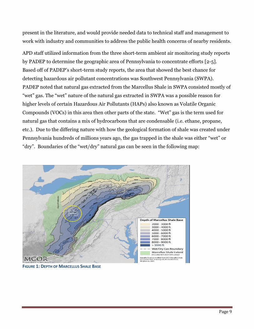
PADEP noted that natural gas extracted from the Marcellus Shale in SWPA consisted mostly of
“wet” gas. The “wet” nature of the natural gas extracted in SWPA was a possible reason for
higher levels of certain Hazardous Air Pollutants (HAPs) also known as Volatile Organic
Compounds (VOCs) in this area then other parts of the state. “Wet” gas is the term used for
natural gas that contains a mix of hydrocarbons that are condensable (i.e. ethane, propane,
etc.). Due to the differing nature with how the geological formation of shale was created under
Pennsylvania hundreds of millions years ago, the gas trapped in the shale was either “wet” or
“dry”. Boundaries of the “wet/dry” natural gas can be seen in the following map:
FIGURE 1: DEPTH OF MARCELLUS SHALE BASE FIGURE 1: DEPTH OF MARCELLUS SHALE BASE

Page 10
West of the “wet/dry” natural gas line contains “wet” natural gas and east of the line contains
“dry” natural gas. “Dry” natural gas is ready for distribution almost immediately because the
condensable liquids are not present. Based on the conclusion PADEP came to regarding “wet”
gas, in addition to seeing where the “wet” natural gas is being extracted, EPA Region 3 decided
to concentrate efforts looking for a monitoring site in SWPA.
In determining a location to monitor, APD collected information on compressor stations in the
SWPA area. Some of the information used in determining a suitable location to site the
monitors were: # of compressor engines, dehydrators present, flare operating, etc. When
looking at various compressor stations throughout SWPA, it was noted that the Brigich
compressor station had: five compressors, a dehydrator, reboiler, three condensate tanks two
diesel generators, blowdown vent and a flare. Since the Washington Co. area being monitored
is located in the “wet gas” part of Pennsylvania, the “wet gas” will pass through and be
processed to remove the condensates in the Brigich facility. The size of the facility being fairly
large with five compressors and three condensate tanks was a factor for monitoring at this
location. Additionally, compressor engines and condensate tanks have been sources of concern
for air pollution. With condensate tanks, “fugitive” gas escaping the controls may be a concern.
FIGURE 2: STATE OF PENNSYLVANIA AND WASHINGTON COUNTY

Page 11
However, monitoring could determine if residents living nearby this facility are being impacted
by VOCs emissions escaping the designed controls.
There is a neighborhood/development that is ~0.3 miles away in the downwind direction and
other homes are within 0.25 miles of the compressor station.
It was observed that the Brigich compressor station is located in an open field at an elevation
maxima compared to the residential properties. Having the compressor station located at an
elevation maximum compared to the nearby surrounding area in close proximity to residential
properties allowed for better pollution dispersion. Pollution dispersion from Brigich would be
hindered if the facility was located in a valley and houses were above the station like what was
observed at other compressor stations in Washington County.
Methods and materials
Specific Aims: Aim 1: To explore and assess the potential chemical exposures from air emissions to people
living nearby to Oil and/or Gas Production Activities operations;
Aim 2: To compare this data to comparison values and identify any compounds that are
uniquely detected in the ambient air near Oil and/or Gas Production Activities operations,
specifically a compressor station.
As part of this monitoring initiative, the information collected was used to evaluate the need to
mitigate exposures, conduct additional air assessments and identify whether air modeling is
needed for this location. This monitoring was an important element for APD to assess the
potential air exposures from these operations that have at least at present, perceived elevated
risks to public health. In parallel with oil and gas production in Pennsylvania, community
members located near drill pads, compressor stations and water and waste impoundments
(some over six acres in size) had been reporting a perplexing array of health symptoms. While
residential dwellings are in some cases less than 1,000 feet from these industrial activities,
residential exposure data (particularly for the air pathway) are lacking. This exposure
assessment utilized a study design currently used in the literature that provided the most
opportunities and flexibility to analyze the data collected. This will enhanced the Region’s

Page 12
ability to address public health questions raised by oil and gas operations in the Region; by
developing monitoring protocols and capacity to assess these specific exposures. These
chemicals include H2S, benzene, formaldehyde, PAHs, including naphthalene, aldehyde,
acrolein, propylene glycol, toluene, xylenes, ethyl benzene and hexane. Aldehydes and glycols
are frack fluids and are composed of a number of constituents, each with a specific purpose
during the drilling process. Biocides are also added to the frack fluid to control bacteria growth
down the well.
This study provides needed data for technical staff and management to work with industry and
communities to address the public health concerns of nearby residents.
Project Objectives
EPA Region 3 measured the following chemicals found in Table 2 at residential locations
surrounding the compressor station. EPA Region 3 collected ambient air monitoring samples
to determine if concentrations of certain VOCs and PM2.5 are at or above levels of concern. A
priority of the NGAAMI was for the samples to be collected on residential properties that are
nearby, or adjacent to, a longer-term natural gas extraction processes/facilities. Longer-term
operating facilities are the focus of this initiative compared to an active drill site which may
only be active for a month or two. Once monitors were sited and samples were collected the
data was intended to be used for: 1) determining impacts, if any, on the ambient air quality at
residential locations that are in close proximity to natural gas extraction processes; 2)
determining if additional action is necessary by EPA, state, and/or local agencies to ensure the
levels of pollutants are detected at safe levels. This initiative was a collaborative effort with the
Agency for Toxic Substances and Disease Registry (ATSDR) in Region 3. Our VOC and PM2.5
results were provided to ATSDR to include in their Health Consultation, Exposure
Investigation not yet released.

Page 13
Project Design
Site Selection
EPA Region 3 chose a sampling location in Southwest PA (Washington Co.) to collect VOC and
PM2.5 samples (see air monitoring sites Figures 2 through 4 in Google Earth map). The location
was near a compressor station. At the sampling location, there were three monitoring sites
collecting samples. For Quality Assurance (QA) purposes, one monitoring site was collocated
to conduct sensitivity analysis. A background site was selected where samples were collected
for both VOCs and PM2.5. A 3-meter meteorological tower was operating at one site of the
three sampling location.
Monitor Siting: Although there was no requirement to follow the Code of Federal
Regulations (CFR) siting criteria in 40CFR, Part 58 App. E, every attempt was
made that could be implemented on the sampling location. The following
criteria were used to select the monitoring locations:
Not impacted by nearby influences other that the compressor station or frack-
water impoundment;
Not in an area where air flow is obstructed;
Place sampler inlets at a representative height;
Practical location for security of equipment;
Set monitors to 0.5 to 1.5m above the ground and adjacent to areas of interest;
Away from all minor sources such as roads, farm equipment as reasonably
practical, >100 m from fuel and farm equipment storage areas;
Inside the immediate area of oil and gas facility ( within 1/3 mile) to capture
“worst-case” sampling if possible;
At least 20 m from the nearest tree canopy;
Away from buildings and areas that disrupts air flow;
In flat terrain where possible.

Page 14
FIGURE 3: GOOGLE EARTH VIEW OF THE BRIGICH COMPRESSOR STATION, CHARTIERS TOWNSHIP, PA
VOC Canister Sampling and Analysis
EPA Region 3 personnel deployed and collected 24-hour ambient air samples from pre-
designated monitoring site locations using 6-liter stainless steel summa canisters. Each
canister was equipped with a restrictive orifice at a flow range between 2-4 mL/min and
sampled for a duration of 24 hours. An in-line timer was also used to ensure samples start and
stop at the same time. All samples were submitted to the EPA Region 3’s Office of Analytical
Services and Quality Assurance (OASQA) laboratory in Fort Meade, MD for VOC analysis.
There were at least eight canisters delivered to the lab after each scheduled sampling day. The
OAQSA lab has a list of determined Minimum Detection Limits (MDL) for the compounds that
were analyzed by EPA Compendium Method TO-15 was used for analysis. The OAQSA lab has
also set the reporting limit at 0.5 parts-per-billion-volume (ppbv). All canisters and flow rate

Page 15
orifices were certified clean by the OAQSA lab prior to being shipped back out to the field. All
results were reported to EPA Region 3 in micrograms per cubic meter (ug/m3) and ppbv.
PM2.5 Sampling and Analysis
EPA personnel collected 24-hour PM2.5 samples from one predetermined air monitoring site at
the compressor station location. The PM2.5 monitoring sites at the compressor station location
was collocated. PM2.5 samples were collected using Airmetrics MiniVol™ TAS. Ambient air
was sampled at 5-liters/per minute and PM2.5 was collected on a polytetrafluoroethylene
(PTFE) Teflon 46.2 millimeter (mm) filter. All sample filters were submitted to the Allegheny
County Health Department (ACHD) in Pittsburgh, PA for filter mass measurement. (Note: The
Airmetrics MiniVol™ TAS is not a PM2.5 Federal Reference Method (FRM) or Federal
Equivalent Method (FEM).)
Meteorological Monitoring
Wind Speed – EPA Region 3 utilized PADEP wind speed and wind direction data that was
collected during the course of NGAAMI. However, PADEP had a sampling location with
meteorology equipment established on a property nearby Site #1 before EPA Region 3 was able
to get out into the field. Since PADEP installed meteorological equipment (PADEP met
equipment was purchased & used during the EPA School Air Toxic Monitoring initiative) at a
site three houses away from EPA’s Site #1, EPA Region 3 decided not to install a meteorological
tower and instead used PADEP’s data.
Sampling Schedule
Monitors at NGAAMI sites collected samples on a 1 in every 3 day schedule over four months
starting on August 4, 2012 and ending on November 28, 2012. At least 30 valid samples were
collected at each of the site locations according to the approved QAPP approved (June 2012).

Page 16
TABLE 1 EPA REGION 3 VOLATILE ORGANIC COMPOUNDS VALID SAMPLING DAYS
Privacy and participation consent
The only personally identifiable data during this initiative were the adult names and the
addresses of the consenting participants. Names will only be used for direct contact by EPA
for reporting of results. The identifiable data will not be used in any reports or any data sets
Sampling Event Day
Site 1 Site 2 Site 2 Collocated
Site 3 Background (Florence)
08/04/2012 X X X X X 08/07/2012 X X X 08/10/2012 X X X X X 08/13/2012 X X X X X 08/16/2012 X X X X 08/25/2012 X X 08/28/2012 X X X X X 08/31/2012 X X X X 09/03/2012 X X X 09/06/2012 X X X X X 09/09/2012 X X X X 09/12/2012 X X X X 09/15/2012 X X X X 09/19/2012 X X X X 09/22/2012 X X X X 09/24/2012 X X X X X 09/27/2012 X X X X X 09/30/2012 X X X X 10/03/2012 X X X X 10/06/2012 X X X 10/09/2012 X X 10/12/2012 X X X X 10/15/2012 X X X X X 10/17/2012 X X X X X 10/19/2012 X X X X X 10/22/2012 X X X 10/25/2012 X X X X X 10/28/2012 X X 10/31/2012 X X X 11/03/2012 X X X X X 11/06/2012 X X X X 11/09/2012 X X 11/12/2012 X X X X X 11/15/2012 X X X 11/17/2012 X X X X 11/19/2012 X X X X 11/25/2012 X 11/27/2012 X X X 11/28/2012 X
Total 30 31 27 30 30

Page 17
produced for this initiative. Consenting participants’ names and addresses were stored in a
password-protected computer. Consent forms were kept in a locked filing cabinet at the EPA
Region 3 office. Participants will not be compensated for their time.
Informed Consent Procedures
If participants indicated a willingness to allow air monitoring/sampling near or on their
property, EPA personnel explained the exposure investigation objects and obtained written,
informed consent, including contact information.
Description of Geographic Area
Demographics Washington County is located in southwestern Pennsylvania, near the Pennsylvania and West
Virginia state boundaries and is a medium sized county of approximately 207,820 people. The
2010 Census reported median household income for 2006-2010 is $49,687 [6]. There are
106,853 women (51.4%) and 100,709 men (48.5%) with a median age of 43.2 years. The
percentage of population in Washington County is predominately White (196,021) with the
following breakdown of African American (6,822), Asian (1,358) and American Indian and
Alaska Native (213)
Data Structure
Lab Results Contaminants were listed by their chemical name as well as CAS Registry Number (a unique
numerical identifier used because a chemical compound can have more than one descriptive
name). This CAS Number was used as the compound ID. Furthermore, each compound within
each sample ID could have up to two entries. Each was listed as a separate line observation.
This dual entry per ID was due to the result units- concentration levels were listed in ppbv and
micrograms per cubic meter (mg/m3). This was necessary to compare against the health and
safety threshold limits which were available in one unit of measurement or the other but
possibly not both. However, there were certain instances in which the lab was only able to give

Page 18
a tentative measurement value in which case they did not elect to make the conversion from
ppbv to ug/m3. Additionally, other variables which were specific to each compound ID, result
value and result unit were also provided and used in the analysis: Value Type (Actual or
Estimated), Reportable Result (Yes or No), Result Type Code (SC, SUC, TIC, TRG), Lab
Qualifiers (multiple options), Result Comment, Reporting Detection Limit, and Quantitation
Limit. This longitudinal dataset was provided in a “univariate” or “long” form with one column
of result values and one column for each of the other variables which included many repeating
values (i.e. Sample ID, location, date, result unit).
Meteorological Data
An average wind direction and speed was provided for each hour of each day of observation.
After review of the PADEP meteorological data, some of the wind speed data showed values
that would only occur in extreme weather events. It was concluded that these “questionable”
wind speed data should not be used in wind rose calculations after comparing those wind
speed values with National Weather Service (NWS) data from Pittsburgh International Airport
(PIT). EPA Region 3 decided to substitute the “questionable” wind speed data with wind speed
data collected by NWS at PIT. The distance between the two locations is about 11 miles. The
procedure used for handling the “questionable” NGAAMI meteorological data followed the
same method used by EPA’s OAQPS for treating “questionable” meteorological data during the
EPA School Air Toxics initiative (Schools Air Toxics Ambient Monitoring Plan, April 2, 2009
[7].
The wind direction and speed could be averaged to provide an overall direction and speed for a
day, although an overall average speed or direction is not useful for this type of analysis.
Instead the percentage of the day in which the wind moved in the direction towards a location
was calculated. The exact angle from the compressor station to each air sample site was found.
From there a zone of 15 degrees in either direction from the site was calculated. This area was
termed the ‘Zone of Influence’ in which wind would have an effect on the contaminants and
how much of a contaminant might be found in an air sample. These percentages were
provided for each date and at each location. Wind speed was not used in this analysis.
Page 19
A wind rose gives a very succinct but information-laden view of how wind speed and direction
are typically distributed at a particular location. Presented in a circular format, the wind rose
shows the frequency of winds blowing from particular directions. The length of each "spoke"
around the circle is related to the frequency of time that the wind blows from a particular
direction. Each concentric circle represents a different frequency, emanating from zero at the
center to increasing frequencies at the outer circles. The wind rose shown in Figure 5 contains
additional information, in that each spoke is broken down into discrete frequency categories
that show the percentage of time that winds blow from a particular direction and at certain
speed ranges. All wind roses shown here use 16 cardinal directions, such as north (N), NNE,
NE, etc. The percentage indicated at the center of the wind rose indicates the frequency of calm
wind observations.

Page 20
FIGURE 4: WIND ROSE FOR OCTOBER 22, 2013 FROM PADEP ONSITE WEATHER STATION
PM2.5 sampling was completed by EPA personnel over a 4 month period starting on August 4,
2012 and concluding on November 25, 2012. The site was located in the dominant downwind
direction from the Compressor Station. Samples were collected on a 1 in 3 day schedule
Wind Rose
October 22, 2012
PADEP onsite weather station
N
S
W E
No observations were missing.Wind flow is FROM the directions shown.Rings drawn at 10% intervals.Calms included at center.
0.00
0.00 0.00
0.00
0.00
4.17
12.50
8.33
4.17 0.00
8.33
4.17 29.17
29.17
0.00
0.00
0.00
Wind Speed ( Miles Per Hour)
0.1 3 7 12 18 24

Page 21
excluding holidays. Samples were delivered to the Allegheny County, PA laboratory for weight
analysis using the gravimetric method. During the four month period a total of thirty-seven
samples were collected and from those samples thirty-five were valid. The remaining two
samples were invalidated due to failure to meet established field and/or laboratory quality
control criteria. The completeness goal for the monitoring initiative (see NGAAMI QAPP) was
to obtain at least 30 valid samples. EPA attained 100% measurement completeness for the
PM2.5 assessment after samples collected on November 15, 2012 were weighed and validated.
Health and Safety Threshold Values
The EPA assesses toxicity by comparing observed concentration levels against the existing
long-term cancer-causing and non-cancer-causing compounds values used in the School Air
Toxics Initiative by EPA. We also included any threshold values used here for comparison by
ATSDR. It was important that each compound tested in the air samples had at least one
threshold limit for comparison and interpretation. The eight types of limits are: EPA’s Long
Term Non-Cancer and Individual limits and EPA’s Long Term Cancer (presented in both ppbv
and ug/m3 result units); short, chronic, and Texas Commission on Environmental Quality’s
(TCEQ) short-term ESL and long-term ESL limits; and lastly, ATSDR’s Cancer Risk Evaluation
Guides (CREG) (ATSDR and TCEQ limits were presented in only ug/m3). These are shown in
Table 2.

TABLE 2 CANCER-BASED AND NON-CANCER BASED LONG TERM COMPARISON VALUES1,2 *
Target Compound CAS Individual (ppbv)
Long Term-NonCancer
(ppbv)*
Long Term-Cancer
(ppbv)*)
ATSDR
CREG ppbv
ATSDR
acute ppbv
ATSDR chronic ppbv
TCEQ Short-term
ELS (ppbv)
TCEQ-
Long-term ELS (ppbv)
1,1-Dichloroethane 75-34-3
1266.6 - 18.1 - -
- 1000 100
1,1-Dichloroethene 75-35-4
20.2 50.4 - - - - 54 -
1,1,1-Trichloroethane 71-55-6
1832.6 916.3 - - 2000 - - -
1,1,2-Trichloroethane 79-00-5
80.6 73.3 1.2 0.01 - - 100 10
1,1,2,2-Tetrachloroethane
79-34-5
17.5 0.2 - 0.003 - - 10 1
1,2-Dibromoethane 106-93-4
1.6 1.2 0.0 0.0002
- - 0.5 -
1,2-Dichloroethane 107-06-2
66.7 593.0 0.9 0.01 - 600 40 -
1,2-Dichloropropane 78-87-5
43.3 0.9 1.1 - 50 - - -
1,2,4-Trichlorobenzene 120-82-1
269.5 26.9 - - - - 54 5.4
1,2,4-Trimethylbenzene
95-63-6
2034.3 - - - - - 250 25
1,3-Butadiene 106-99-0
9.0 0.9 1.5 0.02 100 - - -
1,3-Dichlorobenzene 541-73-1
6.7 - - - - - 250 25
1,3,5-Trimethylbenzene
108-67-8
2034.3 - -
1,4-Dichlorobenzene 106-46-7
1663.3 133.1 0.4
Benzene 71-43-2
9.4 9.4 4.1 0.04 9 3 - -
Benzyl chloride 100-44-7
27.0 - 0.4 - - - 10 1
Bromodichloromethane
75-27-4
104.5 - - - - - 100 10
Bromoform 75-25-2
1648.0 - 23.4 0.09 - - 5 0.5
Bromomethane 74-83-9
51.5 1.3 - - 50 50 - -
Carbon disulfide 75-15-0
2247.8 224.8 - - - 300 10 -
Carbon tetrachloride 56-23-5
31.9 303.2 1.1 0.03 - 30 20 -

Page 23
Chlorobenzene 108-90-7
2172.4 217.2 - - - - 100 10
Chloroethane 75-00-3
15160.4 3790.1 - - 20000
- - -
Chloroform 67-66-3
102.4 20.1 - 0.009 100 20 - -
Chloromethane 74-87-3
484.3 43.6 - - 500 50 - -
cis-1,3-Dichloropropene
10061-01-
5
3.1 - - 0.06 - 7 10 1
Dibromochloromethane
124-48-1
105.7 - - - - - 2.3 0.23
Dichlorodifluoromethane
75-71-8
475172.5 - - - - - 10000 1000
Ethylbenzene 100-41-4
9212.5 230.3 9.2 - 5000 60 - -
m,p-Xylene 108-38-3/ 106-42-3
690.9 23.0 - - 2000 50 - -
Methyl tert-butyl ether 1634-04-4
1941.6 832.1 105.4 2000 700 - -
Methylene chloride 75-09-2
575.8 287.9 60.5 - - - - 900
Naphthalene 91-20-3
5.7 0.6 0.6 - - 0.7 90 -
o-Xylene 95-47-6
2072.8 23.0 - 2000 50 - -
Propylene 115-07-1
17431.1 - - - - - 1000000
-
Styrene 100-42-5
2113.0 234.8 - - 5000 200 - -
Tetrachloroethene 127-18-4
206.4 2.5 39.8 - 2000 - - 10
Toluene 108-88-3
1061.4 1326.8 - - - - - -
trans-1,2-Dichloroethene
156-60-5
201.8 - - - 200 200 - -
trans-1,3-Dichloropropene
10061-02-
6
3.1 - - 0.06 - 7 10 -
Trichloroethene 79-01-6
1875.0 112.5 9.4 - 2000 - - 10
Trichlorofluoromethane
75-69-4
355972.9 - - - - - 500 -
Vinyl chloride 75-01-4
391.2 39.1 4.3 0.04 500 - - -
cis-1,2-Dichloroethene 156-59-2
- - - - - - 2.3 0.23
Dichlorotetrafluoroethane
76-14-2
- - - - - - 10000 1000
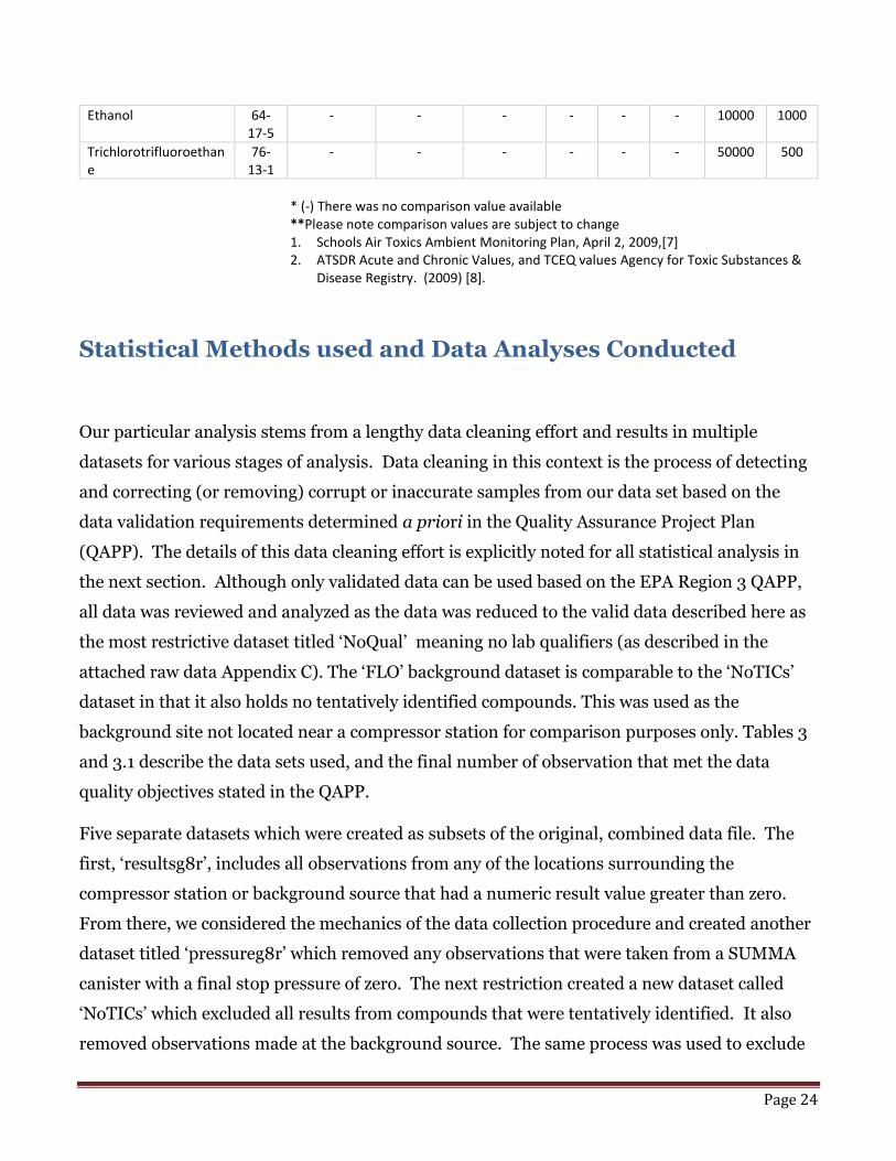
Page 24
* (-) There was no comparison value available **Please note comparison values are subject to change
1. Schools Air Toxics Ambient Monitoring Plan, April 2, 2009,[7] 2. ATSDR Acute and Chronic Values, and TCEQ values Agency for Toxic Substances &
Disease Registry. (2009) [8].
Statistical Methods used and Data Analyses Conducted
Our particular analysis stems from a lengthy data cleaning effort and results in multiple
datasets for various stages of analysis. Data cleaning in this context is the process of detecting
and correcting (or removing) corrupt or inaccurate samples from our data set based on the
data validation requirements determined a priori in the Quality Assurance Project Plan
(QAPP). The details of this data cleaning effort is explicitly noted for all statistical analysis in
the next section. Although only validated data can be used based on the EPA Region 3 QAPP,
all data was reviewed and analyzed as the data was reduced to the valid data described here as
the most restrictive dataset titled ‘NoQual’ meaning no lab qualifiers (as described in the
attached raw data Appendix C). The ‘FLO’ background dataset is comparable to the ‘NoTICs’
dataset in that it also holds no tentatively identified compounds. This was used as the
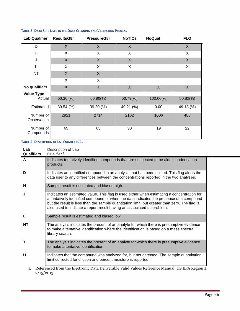
background site not located near a compressor station for comparison purposes only. Tables 3
and 3.1 describe the data sets used, and the final number of observation that met the data
quality objectives stated in the QAPP.
Five separate datasets which were created as subsets of the original, combined data file. The
first, ‘resultsg8r’, includes all observations from any of the locations surrounding the
compressor station or background source that had a numeric result value greater than zero.
From there, we considered the mechanics of the data collection procedure and created another
dataset titled ‘pressureg8r’ which removed any observations that were taken from a SUMMA
canister with a final stop pressure of zero. The next restriction created a new dataset called
‘NoTICs’ which excluded all results from compounds that were tentatively identified. It also
removed observations made at the background source. The same process was used to exclude
Ethanol 64-17-5
- - - - - - 10000 1000
Trichlorotrifluoroethane
76-13-1
- - - - - - 50000 500

Page 25
Tentatively Identified Compounds in the dataset containing data at the background location,
FLO. Past this step, we created another dataset where the compounds were confidently
identified but the result value was an estimated value. Here, in the NoQual dataset, we
excluded any and all observations with a lab qualifier. In summary, the spread of lab qualifiers
can be seen here in Table 3 and 4.
Page 26
TABLE 3: DATA SETS USED IN THE DATA CLEANING AND VALIDATION PROCESS
Lab Qualifier ResultsG8r PressureG8r NoTICs NoQual FLO
D X X X X
H X X X X
J X X X X
L X X X X
NT X X
T X X
No qualifiers X X X X X
Value Type Actual 60.36 (%) 60.80(%) 50.79(%) 100.00(%) 50.82(%)
Estimated 39.54 (%) 39.20 (%) 49.21 (%) 0.00 49.18 (%)
Number of Observation
2921 2714 2162 1006 488
Number of Compounds
65 65 30 19 22
TABLE 4: DESCRIPTION OF LAB QUALIFIERS 1.
Lab Qualifiers
Description of Lab Qualifier 1
A Indicates tentatively identified compounds that are suspected to be aldol condensation products.
D Indicates an identified compound in an analysis that has been diluted. This flag alerts the data user to any differences between the concentrations reported in the two analyses.
H Sample result is estimated and biased high.
J Indicates an estimated value. This flag is used either when estimating a concentration for a tentatively identified compound or when the data indicates the presence of a compound but the result is less than the sample quantitation limit, but greater than zero. The flag is also used to indicate a report result having an associated qc problem.
L Sample result is estimated and biased low
NT The analysis indicates the present of an analyte for which there is presumptive evidence to make a tentative identification where the identification is based on a mass spectral library search.
T The analysis indicates the present of an analyte for which there is presumptive evidence to make a tentative identification
U Indicates that the compound was analyzed for, but not detected. The sample quantitation limit corrected for dilution and percent moisture is reported.
1. Referenced from the Electronic Data Deliverable Valid Values Reference Manual, US EPA Region 2 2/15/2013

Page 27
With increased precision, there is a decrease in the number of observations. This trade-off
associated with excluding observations but increasing precision can be viewed in Table 3. In
general, as the number of observations decreases (excluding FLO), there is an increase in the
percentage of actual values as compared to the estimated values suggesting more reliable
measurements. For comparisons, see the Appendix A (Tables A-2 through A-6) for the list of
compounds by CAS Number in each of the datasets. There are 65 compounds in resultsg8r and
pressureg8r, there are 30 in the noTICs dataset and 19 compounds in the NoQual dataset.
(FLO the background site has 22 compounds.)
We looked at the raw data by viewing a scatterplot of the results of each dataset by days,
however, very small concentration are a challenge to view graphically. To address this, data
was transformed and viewed and analyzed using the log of the results values. Scatterplots are
available in the Appendix A (tables A-7 through A-12). Since this dataset containing no
tentatively identified compounds contains Multi-level clustered data, additional Longitudinal
Data Analysis was completed for VOCs only (see appendix D).
Location 2 and Collocated Location 2
Following this, we conducted a sensitivity analysis comparing the result at Location 2 and
collocated Location 2. This means that two identical sampling instruments were located very
close to each other at the site of interest to detect the measurement error between two samples
collected ambient air very close to each other (see Appendix D for more details). As such, the
data from the collocated sampling instrument could be used as a sensitivity analysis of the
results found. An analysis of variance (ANOVA) was conducted to compare these results.
Analysis of variance is used to describe how the mean of a continuous variable (such as result
value, here) depends on a categorical independent variable (Location 2 and collocated Location
2). ANOVA answers the question: does location have an effect on results? We tested the null
hypothesis and there was no difference between the results and these two locations. See Table
A-18 in Appendix A. With a p-value of 0.95 we could not reject the null hypothesis and
combined the results from the two sections. Scientifically, the results from the two should not
have any real difference.

Page 28
Descriptive Statistics
In order to accurately describe the compounds individually and maintain a summary set, not
all of the 30 compounds with available concentration levels in the NoTICs dataset are analyzed
individually. To determine the number of and most important compounds, all of the results for
each of the 30 given compounds were compared at the compressor station—the contamination
source of interest—against the results at the background source for that same given compound.
We tested the null hypothesis; there was no significant difference in concentration levels
between the contamination source and background source. Only one compound, Toluene
provided a significant result (p = 0.0278), suggesting a difference in concentration levels
between the two sources (Summary Table A-20 and Figure A-1 and A-2, Appendix A).
However, one compound is not enough to describe an entire air sample analysis and better
practice is to use compounds that best demonstrate the characteristics of the data overall.
Instead of using a significance test to determine which compounds to include, frequencies of
counts of each compound are considered. The histogram below visually describes the pattern
of a few compounds that were detected in the samples only a few times and the number of
chemicals that were consistently detected in our samples, these are: Toluene; Ethanol;
Benzene; Chloromethane; Methylene Chloride; Trichlorofluoromethane;
Dichlorodifluoromethane; Methyl Ethyl Ketone. For example, nine compounds had a
frequency count of zero as shone in figure 5. And five compounds were detected 250 times.

Page 29
FIGURE 5: HISTOGRAM SHOWING THE DISTRIBUTION COUNTS OF COMPOUNDS DETECTED

Page 30
Descriptive statistics are provided for the compounds with a frequency counts greater than 100
shown in table 5 due to the bimodal nature of the histogram in figure 5.
TABLE 5: FREQUENCY COUNTS OF THE TOP EIGHT COMPOUNDS
Volatile Organic Compound Frequency of detection
Toluene 254
Ethanol 246
Benzene 222
Chloromethane 252
Methylene Chloride 212
Trichlorofluoromethane 254
Dichlorodifluoromethane 252
Methyl Ethyl Ketone 206
TABLE 6: ANALYSIS OF VARIANCE FOR THE EIGHT MOST FREQUENT COMPOUNDS
Volatile Organic Compound Mean Median Standard
Deviation
Toluene 2.79 1.3 3.6
Ethanol 1.65 1.57 0.86
Benzene 0.33 0.3 0.15
Chloromethane 0.69 0.7 0.14
Methylene Chloride 0.27 0.2 0.2
Trichlorofluoromethane 0.29 0.3 0.06
Dichlorodifluoromethane 0.63 0.6 0.1
Methyl Ethyl Ketone 0.4 0.3 0.34

Page 31
Descriptive statistics within each of these eight compounds in Table 5 and 6 include: an
examination of statistical moments and measures, lab qualifier investigation, collocation
analysis of variance, and analysis of variance for the three location sites around the compressor
station.
At this point, there are no longer any tentatively identified compounds included, but other lab
qualifiers still exist on some of these compounds which speak to the potential estimation of the
reported value even when there is confidence in the determination of the compound itself. To
see where these qualifiers exist, a frequency of lab qualifiers was performed on each compound
(available in the appendix A) and showed that the eight compounds (Table 3 and Table 4) have
very distinct qualifier characteristics.
Sensitivity analysis continues on the collocated sample analysis at location 2. We have already
determined that there is no overall difference between Locations 2 and collocated Location 2
by conducting an analysis of variance, suggesting the data can be combined for these samples.
To ensure the accuracy of this statement, we conducted another analysis of variance sensitivity
analysis of these two locations by individually considering the eight compounds of highest
frequency. We tested the null hypothesis that—for CAS Number 108-88-3—(toluene) there is
no difference between data collected at Location 2 and collocated Location 2. This is completed
separately for measurements in ppbv result units and ug/m3 result units (note: only ppbv
results shown here, ug/m3 results available). This was repeated for the other seven compounds
and the data for each compound for Locations 2 and collocated Location 2was combined. We
did so on a scientific basis knowing that these results would be similar and we expected that
the difference was a result of other factors that would come in future analysis. Lastly, viewing
the box plots suggested some outliers and non-normal data- despite that the results were
already log-transformed. They also demonstrated how different the compound makeup was
for each of the various compounds. Which suggested that future analysis was needed to
consider compounds individually and not concatenate into one large conglomerate of results.
As with Location 2 and collocated Location 2, an Analysis of Variance was performed
comparing the results of a given compound at the three locations strategically placed around
the compressor station. That same ANOVA was repeated for each of these eight compounds.
Recall that this was an analysis of variance, only: we tested the null hypothesis that there was
Page 32
no significant difference among the three locations versus the alternative that at least one
location has significantly different results for the compound of interest. Here again, we
completed the analysis for each compound individually and for each result unit.
Comparison Values
Using the dataset containing only observations with accurate concentration levels, each
individual observation was compared against the EPA and ATSDR threshold values. Some of
those individual values were found to exceed the thresholds. Because of this, we also found the
mean of each compound and compared that mean to the limits of greatest importance. The
ATSDR CREG limit has been included as it is the most conservative and is the most likely to
have observations which exceed those limits. These CREG values are defined by ATSDR as:
“estimated contaminant concentrations…that would be expected to cause no more than one
excess cancer in a million persons exposed over a lifetime.” [1]. In addition, the EPA Long
Term Cancer and Long Term Non-Cancer limits are also included for their importance and
because their threshold values are available in both ppbv and ug/m3 result units. The
compound means are presented as a ratio to the threshold values.
Results and Interpreation
PM 2.5 PM2.5 sample concentrations ranged from 1.0 to 26.5 µg/m3 (see Table 7). PM2.5 daily
concentrations did not exceed the EPA 24-hour standard of 35 µg/m3. The 4 month average
determined during this monitoring initiative was 12.4 µg/m3, there is insufficient data to
determine whether the annual PM2.5 concentration at this site would exceed the EPA annual
primary standard of 12 µg/m3. For regulatory purposes 3 complete years of PM2.5 data is
required.

Page 33
TABLE 7: SUMMARY OF RESULTS (PM 2.5, 24-HR STANDARD = 35 UG/M3)
Sampling Date Result (µg/m3)
8/4/2012 22.3
8/7/2012 17.7
8/10/2012 13.7
8/13/2012 15.6
8/16/2012 21.4
8/19/2012 1
8/22/2012 16.8
8/28/2012 15.2
8/31/2012 15.8
9/3/2012 13.7
9/6/2012 18.9
9/9/2012 10.6
9/12/2012 13.9
9/15/2012 12.2
9/19/2012 6.4
9/22/2012 14.5
9/25/2012 10.6
9/28/2012 11.2
9/30/2012 10.2
10/3/2012 12.8
10/6/2012 5.8
10/9/2012 10
10/12/2012 8.4
10/15/2012 5.5
10/17/2012 26.5
10/19/2012 9.1
10/22/2012 16
10/25/2012 16.1
10/28/2012 0.9
10/31/2012 1.6
11/3/2012 5
11/6/2012 10.2
11/9/2012 18.6
11/12/2012 11.2
11/15/2012 15.9
Average Concentration: 12.4 µg/m3

Page 34
Comparison Values: Hazardous Air Pollutants [9]
There were no individual concentration values that exceeded a threshold EPA Long Term
Cancer limits and most fell below the limits both individually and as the calculated mean
concentration. The following compounds did have calculated means that exceeded the ATSDR
CREG limit. When interpreting these results, we must recall that we only required a
compound to have one limit for comparison: not all compounds are compared against each
type of limit. 1,2-Dichloroethane (86.67), Chloroform (66.67), Benzene (14.52) and Methylene
Chloride (1.5) each had means greater than the ATSDR CREG limit at the ratios listed in the
parentheses.
Ethylbenzene (0.09), Benzene (0.14) and Trichloroethylene (0.13) had means below the EPA
Long Term Cancer threshold limits in ug/m3 at the ratios listed. More comparisons were
possible in ppbv results units for the EPA Long Term Cancer limits and these had mixed
results. 1,2-Dichloroethane (0.96), Ethylbenzene (0.09), Benzene (0.14), and Methylene
Chloride (0.01) fell below. Though three fall far below the threshold limit, 1,2-Dichloroethane
falls just short of a 1.0 ratio which may be of concern since it is close but not exceeding any
threshold limits. The mean and following ratio is based on the five different values of 1,2-
Dichloroethane that were found. More compounds were available to compare against the EPA
Long Term Non-Cancer limit (ug/m3 and ppbv). Each of the twelve which has limits to
compare against- Ethylbenzene, Styrene, 1,4-Dichlorobenzene, 1,2-Dichloroethane, m,p-
Xylene, Toluene, Chloroform, Benzene, Chloromethane, Methylene chloride, Carbon disulfide,
and o-Xylene- had ratios which fell below 0.1 (See table A-20 in Appendix B.)
The longitudinal analysis also found six of these eight compounds excluding Chloromethane
and Trichlorofluoromethane were statistically significant and were found most frequently at all
three locations support the descriptive statistic findings presented above and are different from
background [9].

Page 35
Conclusion
Residents in the surrounding counties near natural gas extraction, processing and
distribution activities have raised ambient air quality questions and concerns.
Measuring the levels of pollutants in the ambient air around these processes helped EPA
to understand whether the air quality posed any health concerns to residents living in
close proximity to the Brigich Compressor Station in Washington County, PA. EPA
collected data of sufficient quality and quantity in order to make a preliminary
assessment for any potential air pollutant impacts surrounding the Brigich Compressor
Station. As stated in the NGAAMI QAPP, using “if…then…” statements, EPA defined the
following decision rules as a basis for determining possible response actions:
“If the ambient air monitoring data in combination with other information for an
area indicate the need for action to reduce air concentrations of or exposures to air
contaminants, then EPA will work with the appropriate agencies on options for
such actions in outdoor air.
If the available monitoring data and other information are insufficient to support a
conclusion in this regard, then additional data collection may be pursued.
If the available monitoring data and other information are sufficient to reach a
conclusion but do not support the conclusion that further action is needed, then
additional data collection will not be pursued.”
EPA Region 3 has determined, based on the ambient air monitoring data (collected by EPA) that
the ambient concentrations near the Brigich Compressor Station in Washington County, PA did
not indicate impacts of potential concern. Furthermore, it was concluded that additional data
collection would not be pursued. The available air monitoring data and other information
provided in this report sufficiently supports this decision.

Page 36
References 1. PA Department of Environmental Protection, Bureau of Oil and Gas Management. (2014).
2. PADEP 2010a. Chemicals Used by Hydraulic Fracturing Companies in Pennsylvania for
Surface and Hydraulic Fracturing Activities. Pennsylvania Department of Environmental
Protection, Bureau of Oil and Gas Management
3. PADEP 2010b. Southwestern Pennsylvania Marcellus Shale Short-Term Ambient Air
Sampling Report. Pennsylvania Department of Environmental Protection
4. PADEP 2011a. Northeastern Pennsylvania Marcellus Shale Short-Term Ambient Air
Sampling Report. Pennsylvania Department of Environmental Protection.
5.PADEP 2011b. Northcentral Pennsylvania Marcellus Shale Short-Term Ambient Air
Sampling Report. Pennsylvania Department of Environmental Protection
6. U.S Census Burear 2010, and 2012. State and County Quick Facts, Data derived from
Population Estimates, American Community Survey, Census of Population and Housing
7. Schools Air Toxics Monitoring Activity (2009): Uses of Health Effects Information in
Evaluating Sample -
http://www.epa.gov/schoolair/pdfs/UsesOfHealthEffectsInfoinEvalSampleResults.pdf
8. Agency for Toxic Substances & Disease Registry. (2009).Public Health Assessments &
Health Consultations. Comparison
Values. http://www.atsdr.cdc.gov/hac/pha/PHA.asp?docid=768&pg=4

Page 37
9. Jervis, Allison. Philip-Tab, Loni., Gross-Davis, Carol Ann. (unpublished thesis) Analyzing
the clustered data of the US Environmental Protection Agency’s Natural Gas Ambient Air
Monitoring Initiative via linear mixed model methods. For completion of master’s degree in
Biostatistics. Drexel University School of Public Health