natural diffusion: hillslope sediment transport
TRANSCRIPT
Intro to Quantitative Geology www.helsinki.fi/yliopisto
Introduction to Quantitative Geology
Natural diffusion: Hillslope sediment transport
Lecturer: David [email protected]
13.11.2017
3
www.helsinki.fi/yliopistoIntro to Quantitative Geology
Goals of this lecture
• Introduce the diffusion process
• Present some examples of hillslope diffusive processes (heave/creep, solifluction, rain splash)
4
www.helsinki.fi/yliopistoIntro to Quantitative Geology
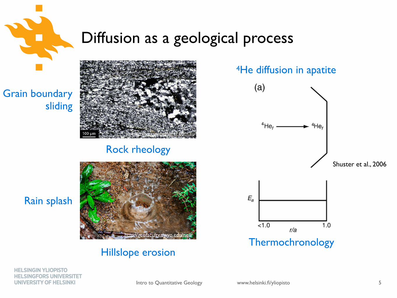
Diffusion as a geological process
5
http://virtualexplorer.com.au
and the mineral's surface (i.e., at the first percolationpoint when damage sites are no longer isolated [10,13])will the net effect be to decrease retentivity.
4.2.3. Quantitative trapping modelGiven that vrd is the volume fraction of radiation damage
sites in a crystal (in cm3/cm3; Fig. 4), then following Farley[3], kt⁎=kt·vrd, where kt is defined as the partition ratio ofhelium “trapped” in sites of radiation damage to helium“free” to migrate through the matrix. Using these relation-ships, and following Crank [30], we find:
DðT ; 4HeÞa2
¼Doa2 d e
−EaRT
kt4þ 1¼
Doa2 d e
−EaRT
kodvrdd eEtRT
! "þ 1
; ð2Þ
where Et is the energy barrier required of a helium atom tomove out of a damage site back into an undamaged regionand, Do and Ea here describe helium diffusion through acrystalline matrix entirely free of radiation damage. If wethen let η be a proportionality constant relating [4He] to thevolume fraction of damage sites (in dimensions gm/nmol)such that vrd=η·[4He], Eq. (2) becomes:
DðT ; 4HeÞa2
¼Doa2 d e
−EaRT
kodgd½4He &d eEtRT
! "þ 1
; ð3Þ
which relatesD /a2 to [4He] at any point in time. By lettingψ=ko·η, the four free parameters for this expression areEa,Et, Do, and ψ.
To determine the best-fit parameters to Eq. (3) wesearched parameter space to minimize the misfit toobservations. This was done as follows. First, a parameterset was selected, and for each sample with its associated[4He] a plot of ln(D /a2) versus 1 /Twas computed. Whenthe effective activation energy is between Ea and Ea+Et
(e.g, for 0.1b [4He]b100 nmol/gm; Fig. 2a) the trappingmodel yields a slightly curving array in this space, so wecomputed 10 values of ln(D /a2) versus 1/T for T between200 and 350 °C, i.e., the temperature range over which weactually measured helium diffusivity. These syntheticpoints were regressed, and the apparent values ln(Do /a
2)and Ea were computed. These were then compared withobservations on that sample, and the total error minimizedweighting the two variables (Ea,Do /a
2) for their variance.(Note that we excluded 5 samples which plot well awayfrom the cluster of remaining samples). In addition, werequired that the resulting range of ln(Do /a
2) and Ea spanthe entire range observed in the dataset. A family of best-fit values were obtained, all of which yielded about thesame degree ofmisfit and all of which yield essentially thesame result upon forward modeling (see below).
4.3. Implications of the revised calibration forthermochronometry
If radiation damage impedes 4He mobility, then theeffective helium diffusion kinetics must change as anapatite evolves through time, and similarly must vary
Fig. 4. A schematic model of the potential influence that isolated sites of radiation damage may have on helium diffusion kinetics. (a) Diffusion of a4He atom across a given distance in a mineral without radiation damage. (b) Diffusion of a 4He atom across the same distance in a mineral withradiation damage; the circle represents a damage site. (c) The same as (b) after more sites of radiation damage accumulate. The upper panels arecartoons of the crystal with the 4He atom motion due to diffusion indicated by the arrows in the vicinity of the crystal surface. Lower panels are plotsof the effective activation energy for diffusion as a function of radial position, r, across a sphere of radius a; r /a=1 corresponds to the crystal surface.Hef is a “free” helium atom located within the undamaged crystal structure, Het is a “trapped” atom located within a site of radiation damage. Ea is theactivation energy for volume diffusion through regions of the crystal entirely free of radiation damage and Et is the energy required of a helium atomto move out of a trap back into the undamaged crystal.
156 D.L. Shuster et al. / Earth and Planetary Science Letters 249 (2006) 148–161
Rock rheology
Hillslope erosionThermochronology
Shuster et al., 2006
4He diffusion in apatite
http://geofaculty.uwyo.edu/neil/
Rain splash
Grain boundarysliding
www.helsinki.fi/yliopistoIntro to Quantitative Geology
General concepts of diffusion
• Diffusion is a process resulting in mass transport or mixing as a result of the random motion of diffusing particles
• Diffusion reduces gradients
• Net motion of mass or transfer of energy is from regions of high concentration to regions of low concentration
• This definition is OK for us, but not perfect
• Hillslope diffusion is a name given to the overall behavior of numerous surface processes that are not themselves diffusion processes based on the definition above
6
www.helsinki.fi/yliopistoIntro to Quantitative Geology
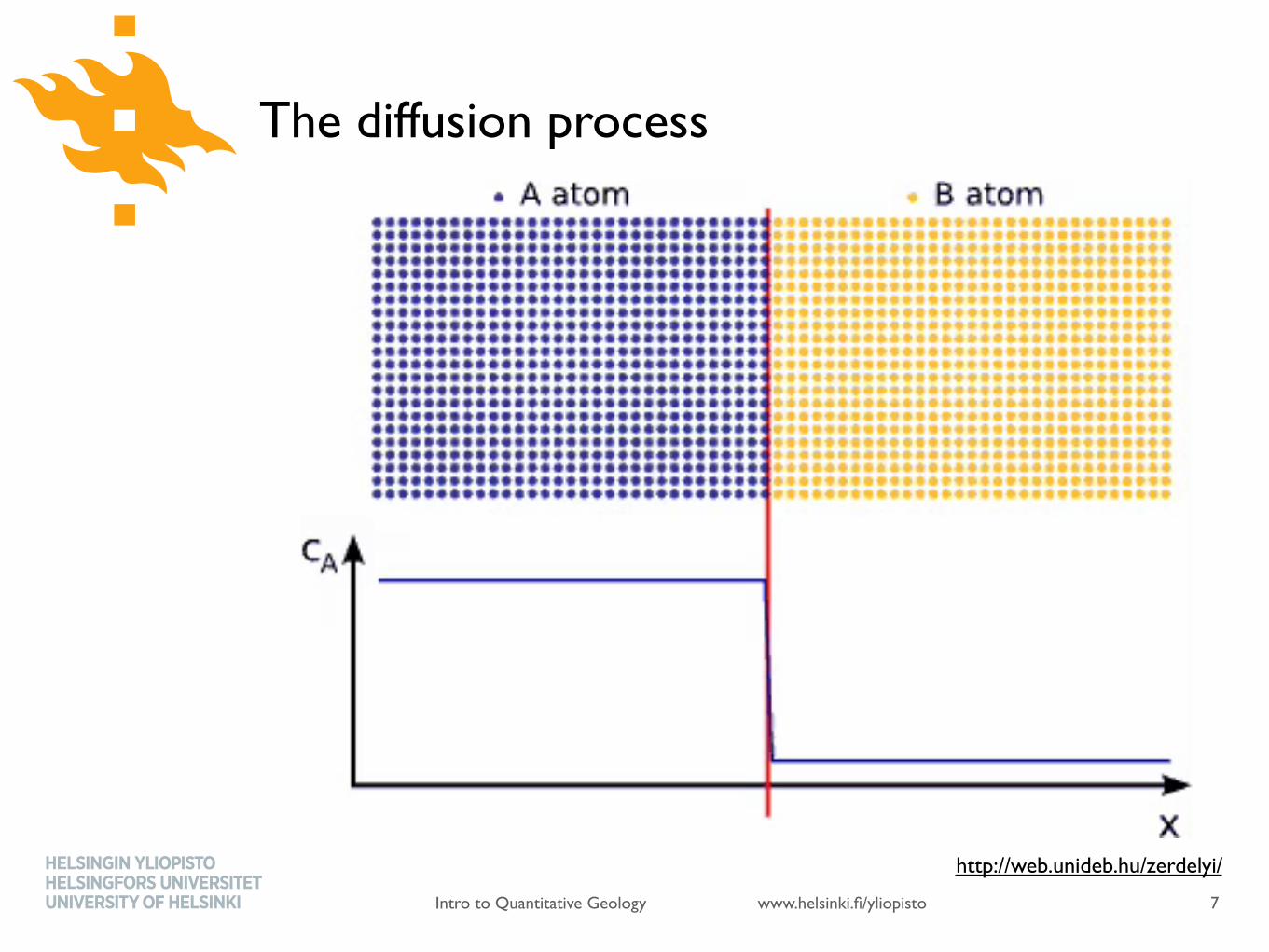
The diffusion process
7
http://web.unideb.hu/zerdelyi/

www.helsinki.fi/yliopistoIntro to Quantitative Geology
The diffusion process
7
http://web.unideb.hu/zerdelyi/
www.helsinki.fi/yliopistoIntro to Quantitative Geology
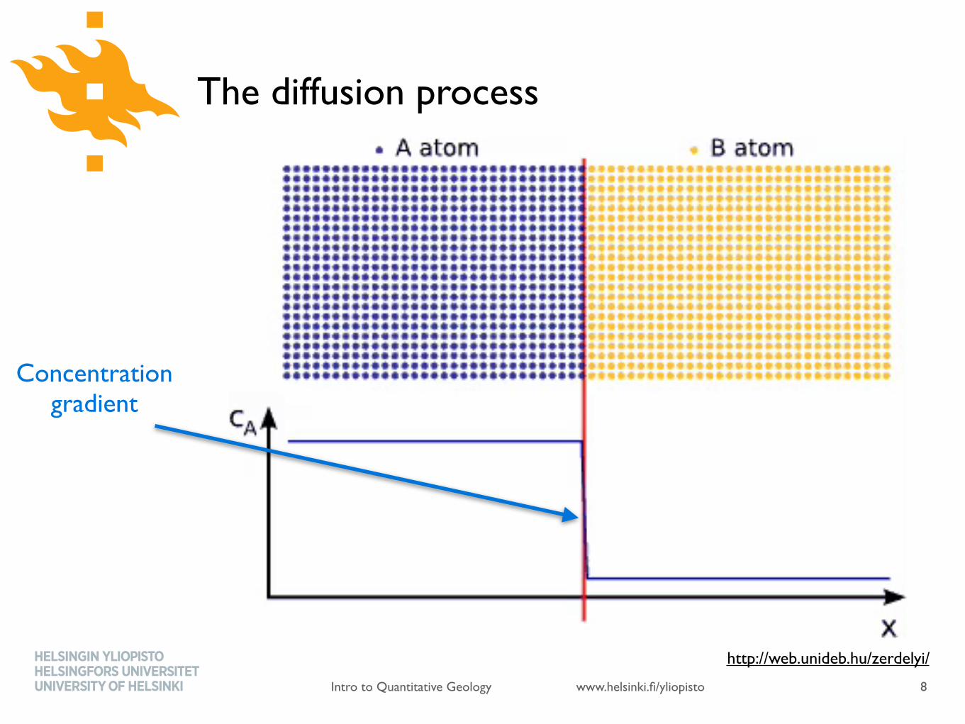
The diffusion process
8
http://web.unideb.hu/zerdelyi/
Concentration gradient

www.helsinki.fi/yliopistoIntro to Quantitative Geology
The diffusion process
8
http://web.unideb.hu/zerdelyi/
Concentration gradient
www.helsinki.fi/yliopistoIntro to Quantitative Geology
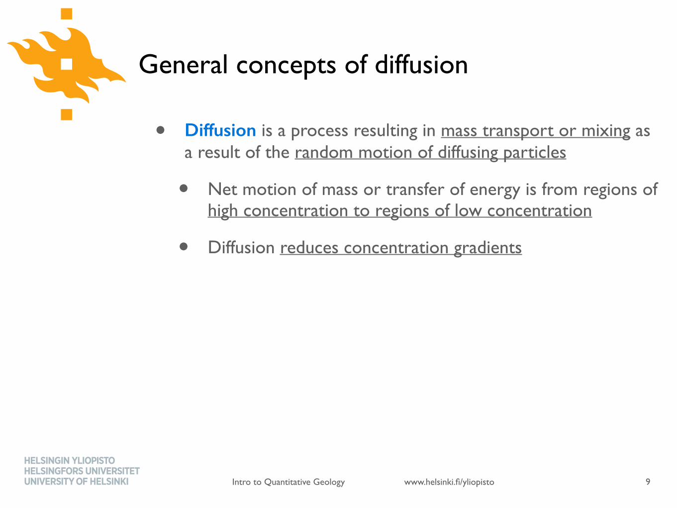
General concepts of diffusion
• Diffusion is a process resulting in mass transport or mixing as a result of the random motion of diffusing particles
• Net motion of mass or transfer of energy is from regions of high concentration to regions of low concentration
• Diffusion reduces concentration gradients
• This definition is OK for true diffusion processes, but there are also numerous geological processes that are not themselves diffusion processes, but result in diffusion-like behavior
• Hillslope diffusion is a name given to the overall behavior of various surface processes that transfer mass on hillslopes in a diffusion-like manner
9
www.helsinki.fi/yliopistoIntro to Quantitative Geology
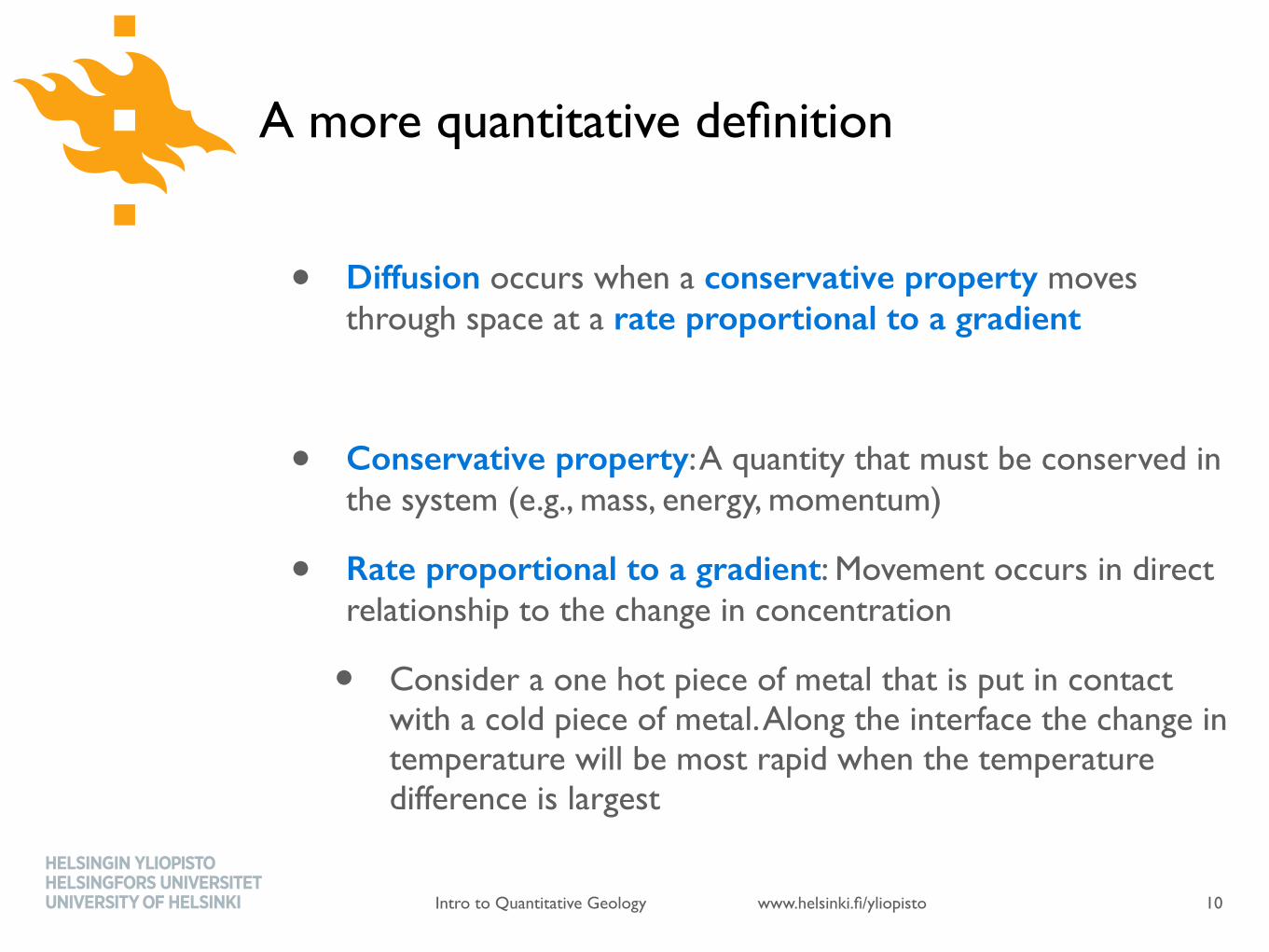
A more quantitative definition
• Diffusion occurs when a conservative property moves through space at a rate proportional to a gradient
• Conservative property: A quantity that must be conserved in the system (e.g., mass, energy, momentum)
• Rate proportional to a gradient: Movement occurs in direct relationship to the change in concentration
• Consider a one hot piece of metal that is put in contact with a cold piece of metal. Along the interface the change in temperature will be most rapid when the temperature difference is largest
10

www.helsinki.fi/yliopistoIntro to Quantitative Geology
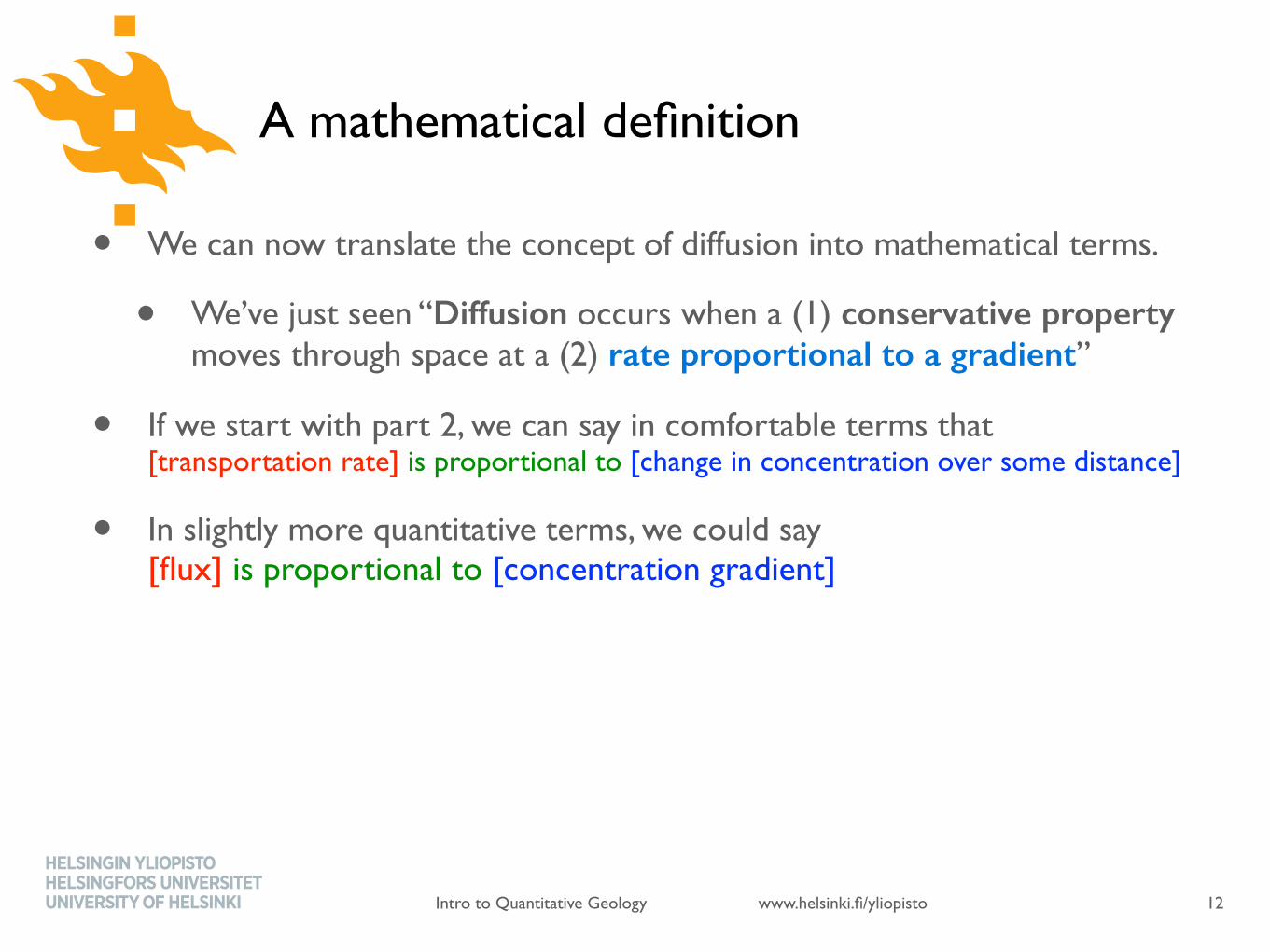
• We can now translate the concept of diffusion into mathematical terms.
• We’ve just seen “Diffusion occurs when a (1) conservative property moves through space at a (2) rate proportional to a gradient”
• If we start with part 2, we can say in comfortable terms that [transportation rate] is proportional to [change in concentration over some distance]
• In slightly more quantitative terms, we could say [flux] is proportional to [concentration gradient]
• Finally, in symbols we can say where ! is the mass flux, ∝ is the “proportional to” symbol, # indicates a change in the symbol that follows, $ is the concentration and % is distance
A mathematical definition
11
q / �C
�x
www.helsinki.fi/yliopistoIntro to Quantitative Geology
• We can now translate the concept of diffusion into mathematical terms.
• We’ve just seen “Diffusion occurs when a (1) conservative property moves through space at a (2) rate proportional to a gradient”
• If we start with part 2, we can say in comfortable terms that [transportation rate] is proportional to [change in concentration over some distance]
• In slightly more quantitative terms, we could say [flux] is proportional to [concentration gradient]
• Finally, in symbols we can say where ! is the mass flux, ∝ is the “proportional to” symbol, # indicates a change in the symbol that follows, $ is the concentration and % is distance
A mathematical definition
12
q / �C
�x
www.helsinki.fi/yliopistoIntro to Quantitative Geology
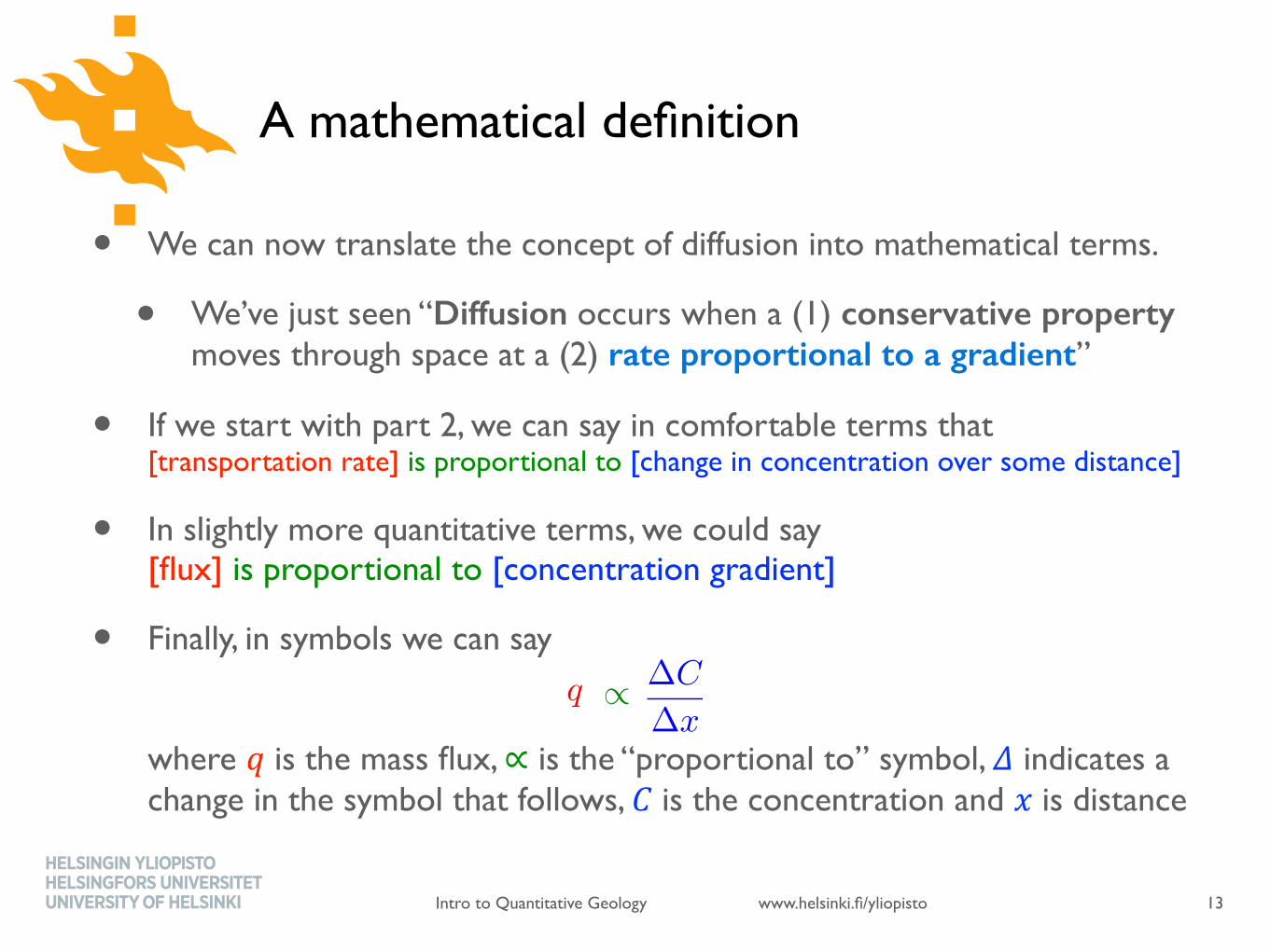
• We can now translate the concept of diffusion into mathematical terms.
• We’ve just seen “Diffusion occurs when a (1) conservative property moves through space at a (2) rate proportional to a gradient”
• If we start with part 2, we can say in comfortable terms that [transportation rate] is proportional to [change in concentration over some distance]
• In slightly more quantitative terms, we could say [flux] is proportional to [concentration gradient]
• Finally, in symbols we can say where ! is the mass flux, ∝ is the “proportional to” symbol, # indicates a change in the symbol that follows, $ is the concentration and % is distance
A mathematical definition
13
q / �C
�x
www.helsinki.fi/yliopistoIntro to Quantitative Geology
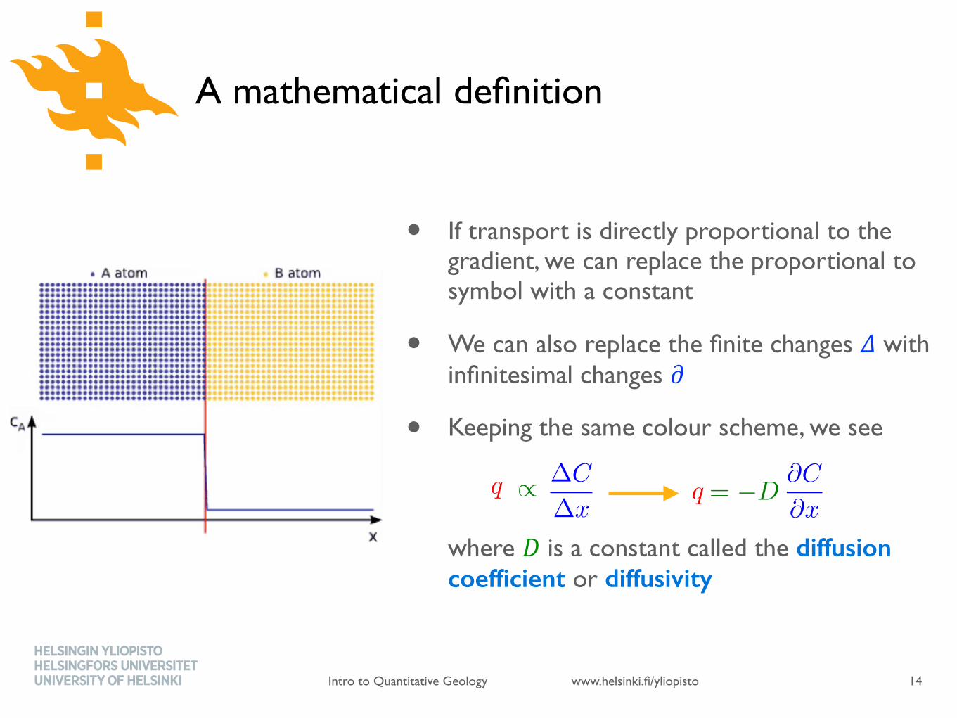
• If transport is directly proportional to the gradient, we can replace the proportional to symbol with a constant
• We can also replace the finite changes # with infinitesimal changes &
• Keeping the same colour scheme, we see where ' is a constant called the diffusion coefficient or diffusivity
A mathematical definition
14
= �D@C
@x
qq / �C
�x

www.helsinki.fi/yliopistoIntro to Quantitative Geology
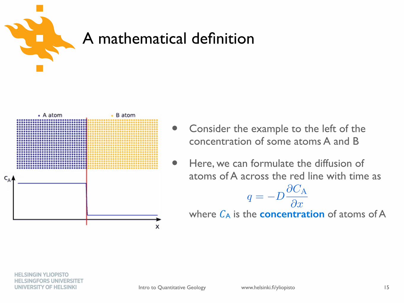
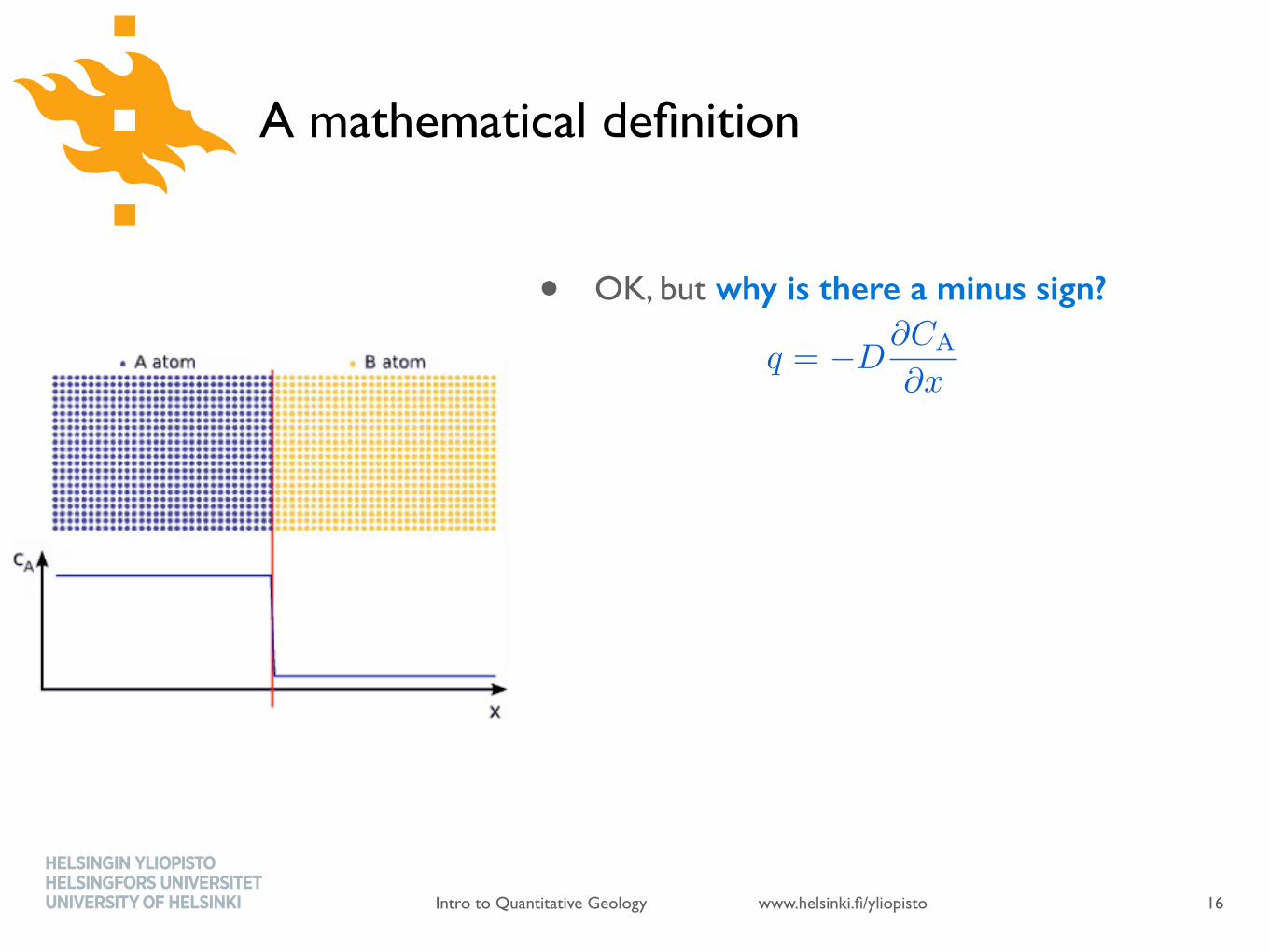
• Consider the example to the left of the concentration of some atoms A and B
• Here, we can formulate the diffusion of atoms of A across the red line with time aswhere $A is the concentration of atoms of A
q = �D
@CA
@x
A mathematical definition
15
www.helsinki.fi/yliopistoIntro to Quantitative Geology
• OK, but why is there a minus sign?
• We can consider a simple case for finite changes at two points: (x1, C1) and (x2, C2)
• At those points, we could say
• As you can see, #$ will be negative while #% is positive, resulting in a negative gradient
q = �D
@CA
@x
A mathematical definition
16
q = �D
�C
�x
q = �D
C2 � C1
x2 � x1
www.helsinki.fi/yliopistoIntro to Quantitative Geology
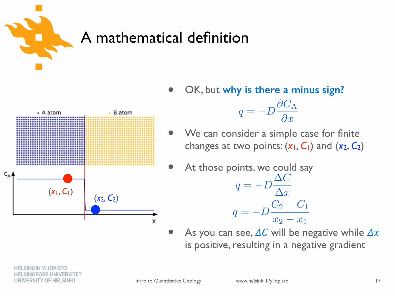
• OK, but why is there a minus sign?
• We can consider a simple case for finite changes at two points: (x1, C1) and (x2, C2)
• At those points, we could say
• As you can see, #$ will be negative while #% is positive, resulting in a negative gradient
q = �D
�C
�x
q = �D
C2 � C1
x2 � x1
A mathematical definition
17
(x1, C1)(x2, C2)
q = �D
@CA
@x
www.helsinki.fi/yliopistoIntro to Quantitative Geology
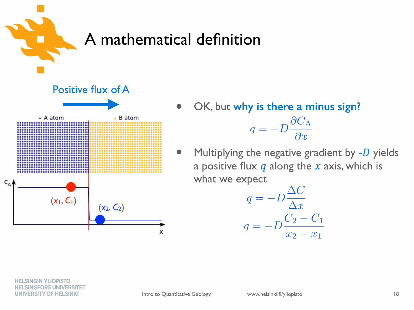
• OK, but why is there a minus sign?
• Multiplying the negative gradient by -' yields a positive flux ! along the % axis, which is what we expect
A mathematical definition
18
(x1, C1)(x2, C2)
Positive flux of A
q = �D
�C
�x
q = �D
C2 � C1
x2 � x1
q = �D
@CA
@x

www.helsinki.fi/yliopistoIntro to Quantitative Geology
• OK, but why is there a minus sign?
• Multiplying the negative gradient by -' yields a positive flux ! along the % axis, which is what we expect
A mathematical definition
18
(x1, C1)(x2, C2)
Positive flux of A
q = �D
�C
�x
q = �D
C2 � C1
x2 � x1
q = �D
@CA
@x
www.helsinki.fi/yliopistoIntro to Quantitative Geology
• We can now translate the concept of diffusion into mathematical terms.
• We’ve seen “Diffusion occurs when a (1) conservative property moves through space at a (2) rate proportional to a gradient”
• This part is slightly harder to translate, but we can say that [change in concentration with time] is equal to [change in transport rate with distance]
• In slightly more quantitative terms, we could say [rate of change of concentration] is equal to [flux gradient]
• Finally, in symbols we can say where t is time
A mathematical definition
19
�C
�t
=�q
�x
www.helsinki.fi/yliopistoIntro to Quantitative Geology
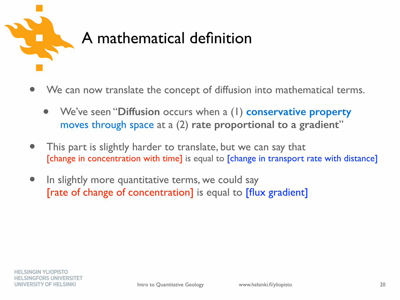
• We can now translate the concept of diffusion into mathematical terms.
• We’ve seen “Diffusion occurs when a (1) conservative property moves through space at a (2) rate proportional to a gradient”
• This part is slightly harder to translate, but we can say that [change in concentration with time] is equal to [change in transport rate with distance]
• In slightly more quantitative terms, we could say [rate of change of concentration] is equal to [flux gradient]
• Finally, in symbols we can say where t is time
A mathematical definition
20
�C
�t
=�q
�x
www.helsinki.fi/yliopistoIntro to Quantitative Geology
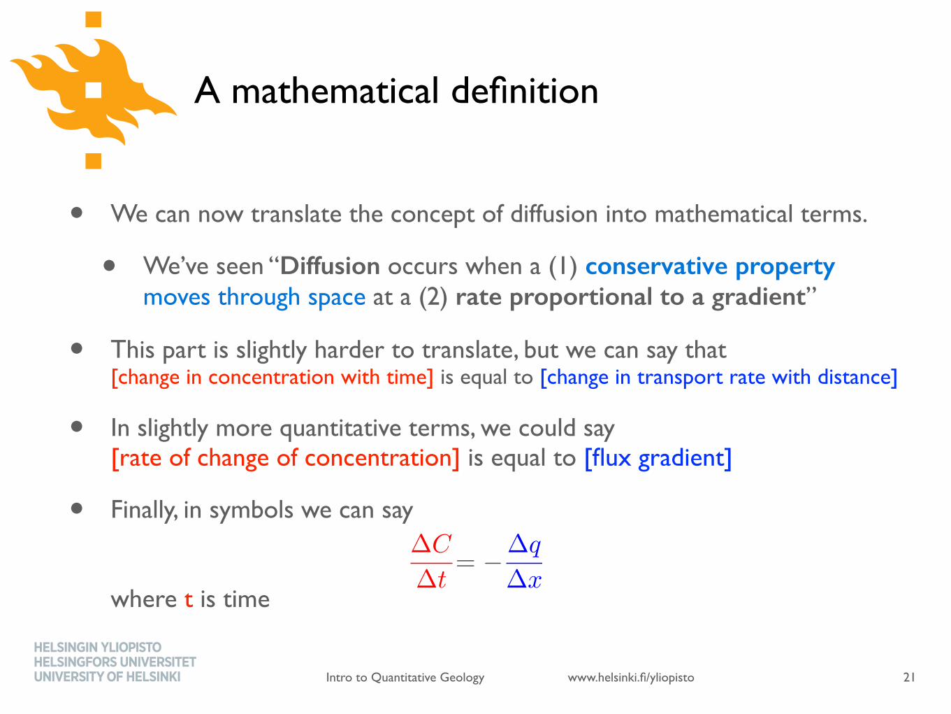
• We can now translate the concept of diffusion into mathematical terms.
• We’ve seen “Diffusion occurs when a (1) conservative property moves through space at a (2) rate proportional to a gradient”
• This part is slightly harder to translate, but we can say that [change in concentration with time] is equal to [change in transport rate with distance]
• In slightly more quantitative terms, we could say [rate of change of concentration] is equal to [flux gradient]
• Finally, in symbols we can say where t is time
A mathematical definition
21
�C
�t
= ��q
�x
www.helsinki.fi/yliopistoIntro to Quantitative Geology
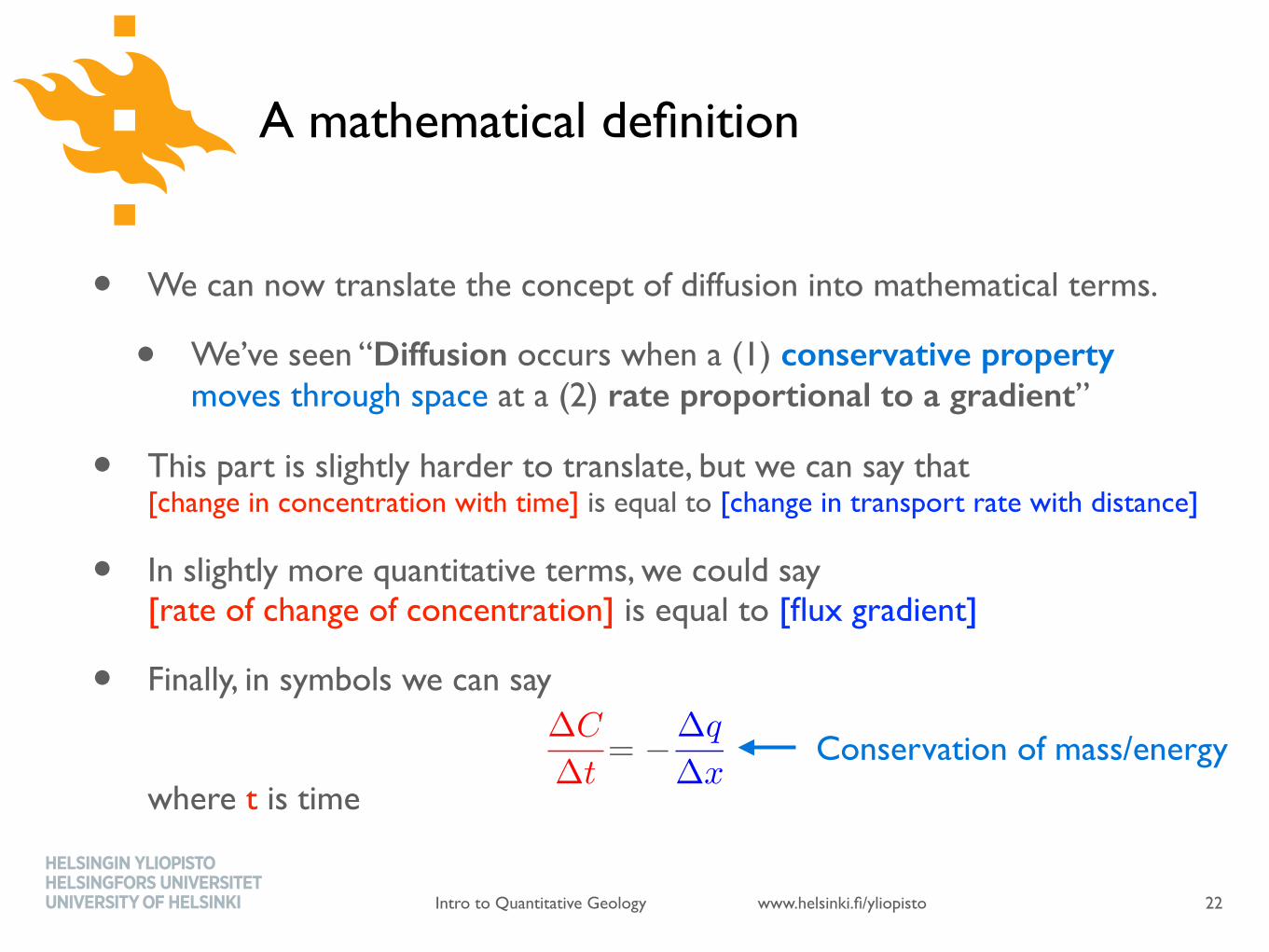
• We can now translate the concept of diffusion into mathematical terms.
• We’ve seen “Diffusion occurs when a (1) conservative property moves through space at a (2) rate proportional to a gradient”
• This part is slightly harder to translate, but we can say that [change in concentration with time] is equal to [change in transport rate with distance]
• In slightly more quantitative terms, we could say [rate of change of concentration] is equal to [flux gradient]
• Finally, in symbols we can say where t is time
A mathematical definition
22
Conservation of mass/energy�C
�t
= ��q
�x
www.helsinki.fi/yliopistoIntro to Quantitative Geology
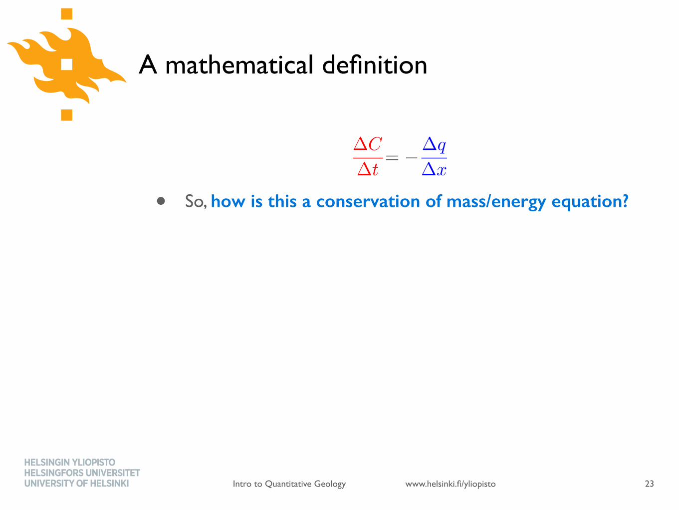
A mathematical definition
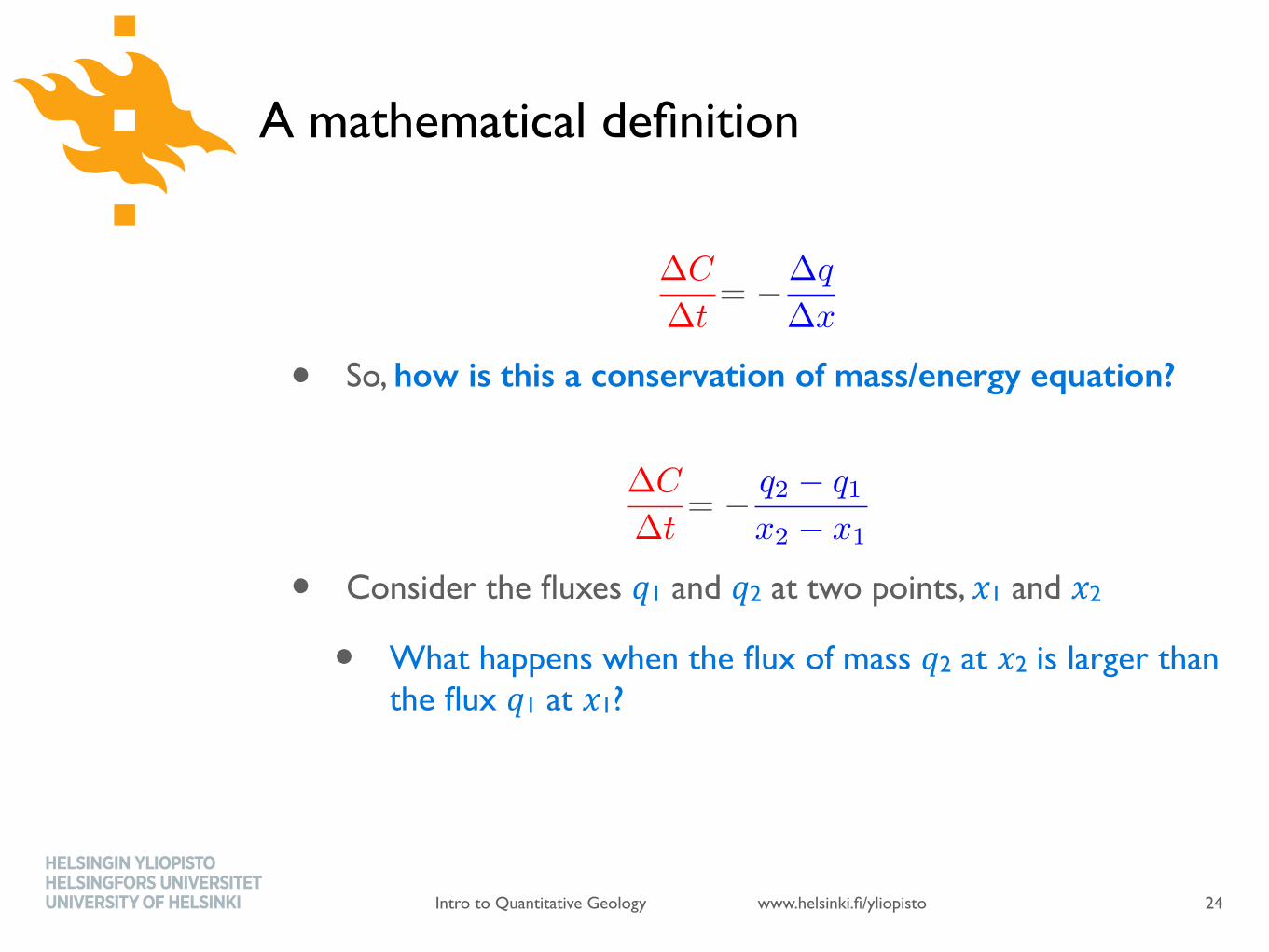
• So, how is this a conservation of mass/energy equation?
• Consider the fluxes !1 and !2 at two points, %1 and %2
• What happens when the flux of mass !2 at %2 is larger than the flux !1 at %1?
23
�C
�t
= ��q
�x
�C
�t
= � q2 � q1
x2 � x1
www.helsinki.fi/yliopistoIntro to Quantitative Geology
A mathematical definition
• So, how is this a conservation of mass/energy equation?
• Consider the fluxes !1 and !2 at two points, %1 and %2
• What happens when the flux of mass !2 at %2 is larger than the flux !1 at %1?
24
�C
�t
= ��q
�x
�C
�t
= � q2 � q1
x2 � x1
www.helsinki.fi/yliopistoIntro to Quantitative Geology
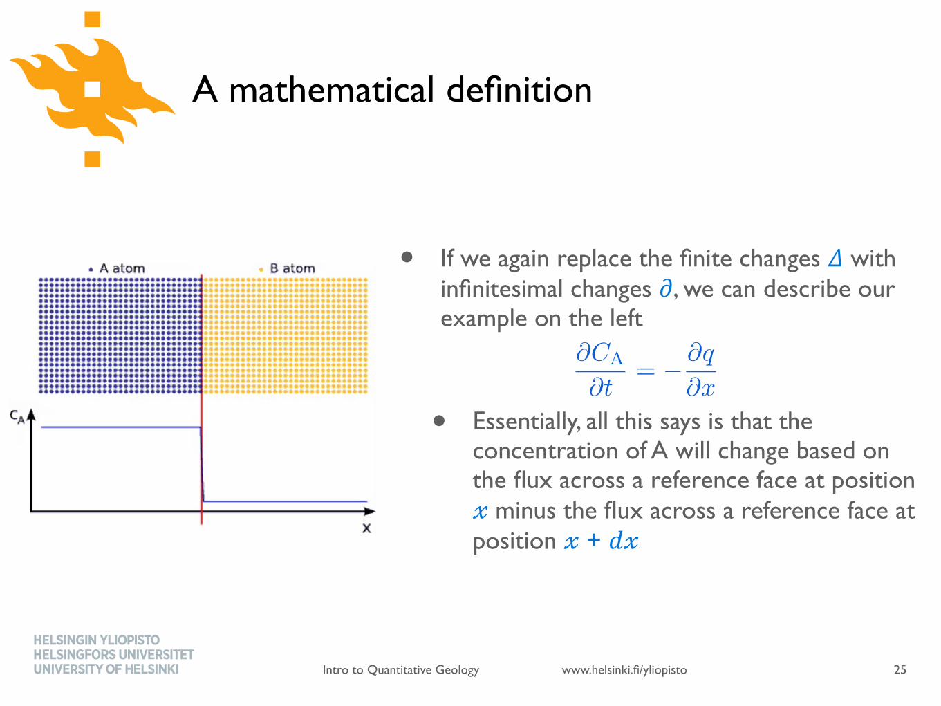
• If we again replace the finite changes # with infinitesimal changes &, we can describe our example on the left
• Essentially, all this says is that the concentration of A will change based on the flux across a reference face at position ( minus the flux across a reference face at position ( + )(
@CA
@t
= � @q
@x
A mathematical definition
25

www.helsinki.fi/yliopistoIntro to Quantitative Geology
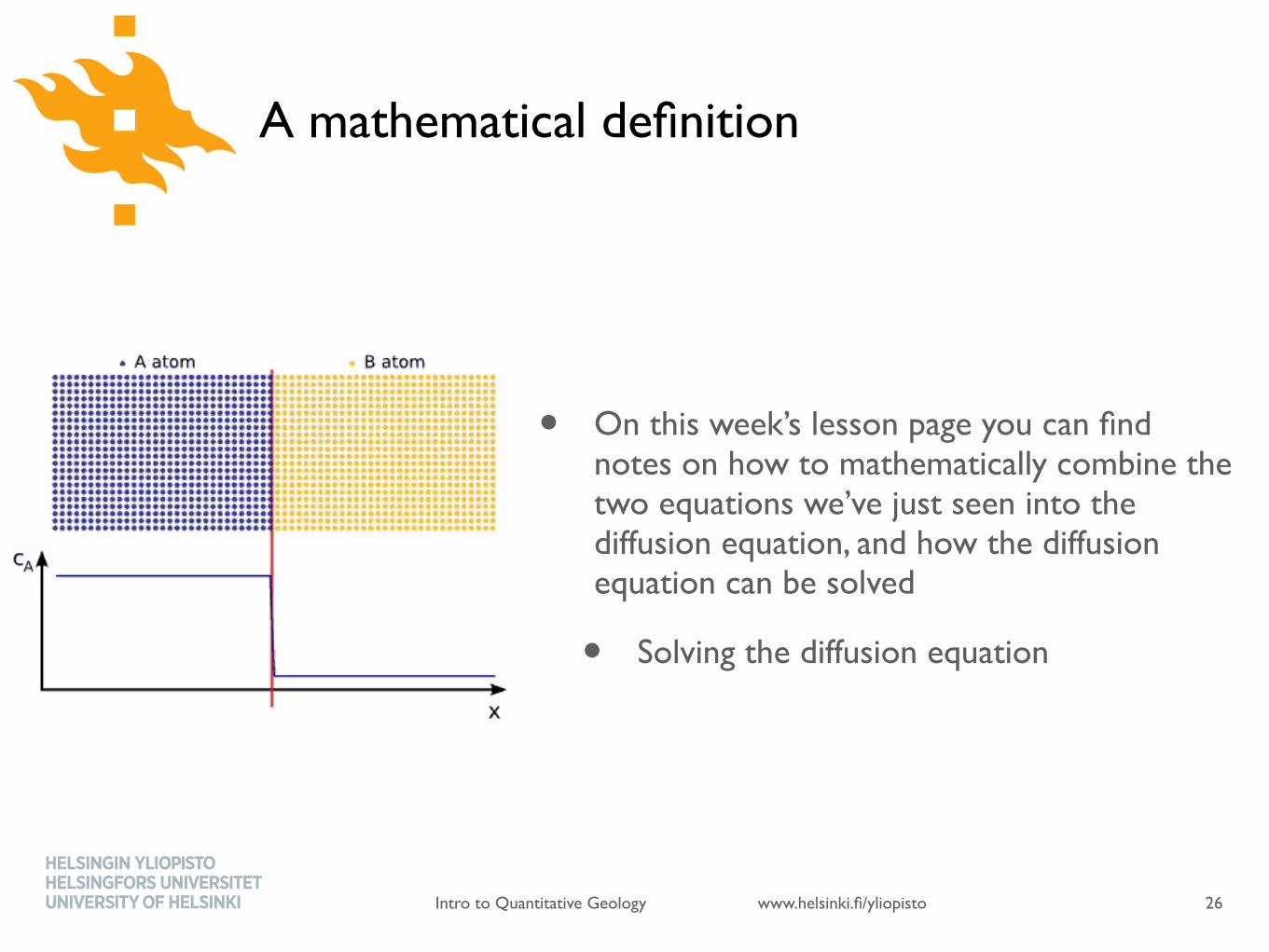
• On this week’s lesson page you can find notes on how to mathematically combine the two equations we’ve just seen into the diffusion equation, and how the diffusion equation can be solved
• Solving the diffusion equation
A mathematical definition
26
www.helsinki.fi/yliopistoIntro to Quantitative Geology
General concepts of diffusion
• So our definitions of diffusion to this point are OK for true diffusion processes, but there are also numerous geological processes that are not themselves diffusion processes, but result in diffusion-like behaviour
• Hillslope diffusion is a name given to the overall behaviour of various surface processes that transfer mass on hillslopes in a diffusion-like manner
27
www.helsinki.fi/yliopistoIntro to Quantitative Geology
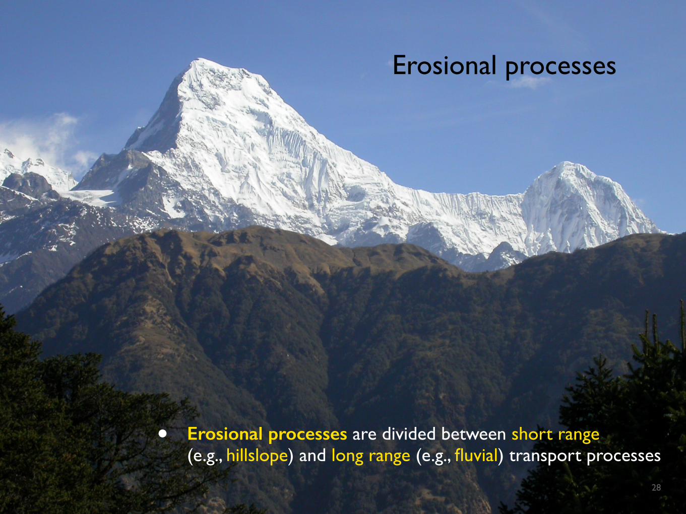
Erosional processes
• Erosional processes are divided between short range(e.g., hillslope) and long range (e.g., fluvial) transport processes
28
www.helsinki.fi/yliopistoIntro to Quantitative Geology
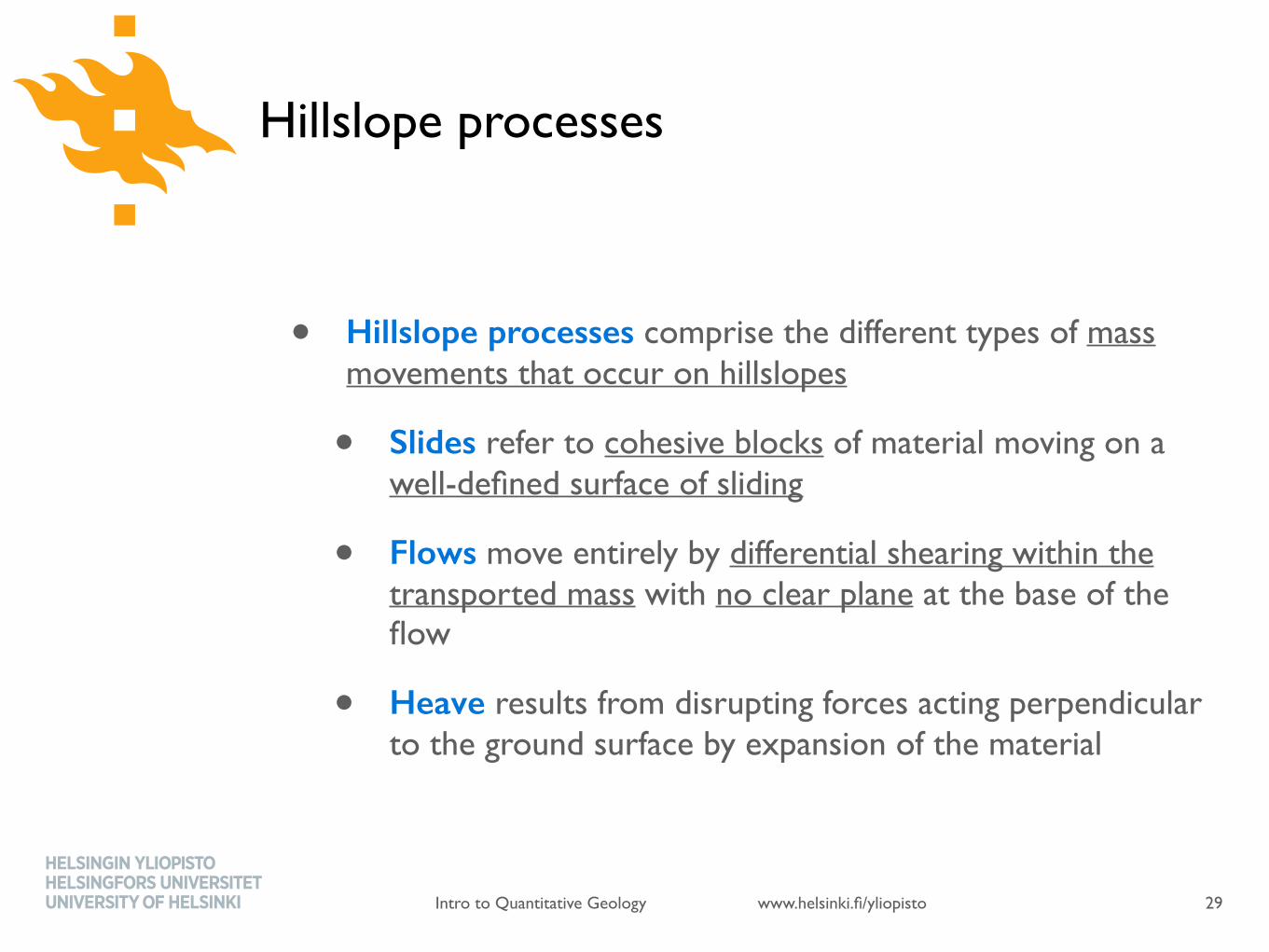
Hillslope processes
• Hillslope processes comprise the different types of mass movements that occur on hillslopes
• Slides refer to cohesive blocks of material moving on a well-defined surface of sliding
• Flows move entirely by differential shearing within the transported mass with no clear plane at the base of the flow
• Heave results from disrupting forces acting perpendicular to the ground surface by expansion of the material
29
www.helsinki.fi/yliopistoIntro to Quantitative Geology
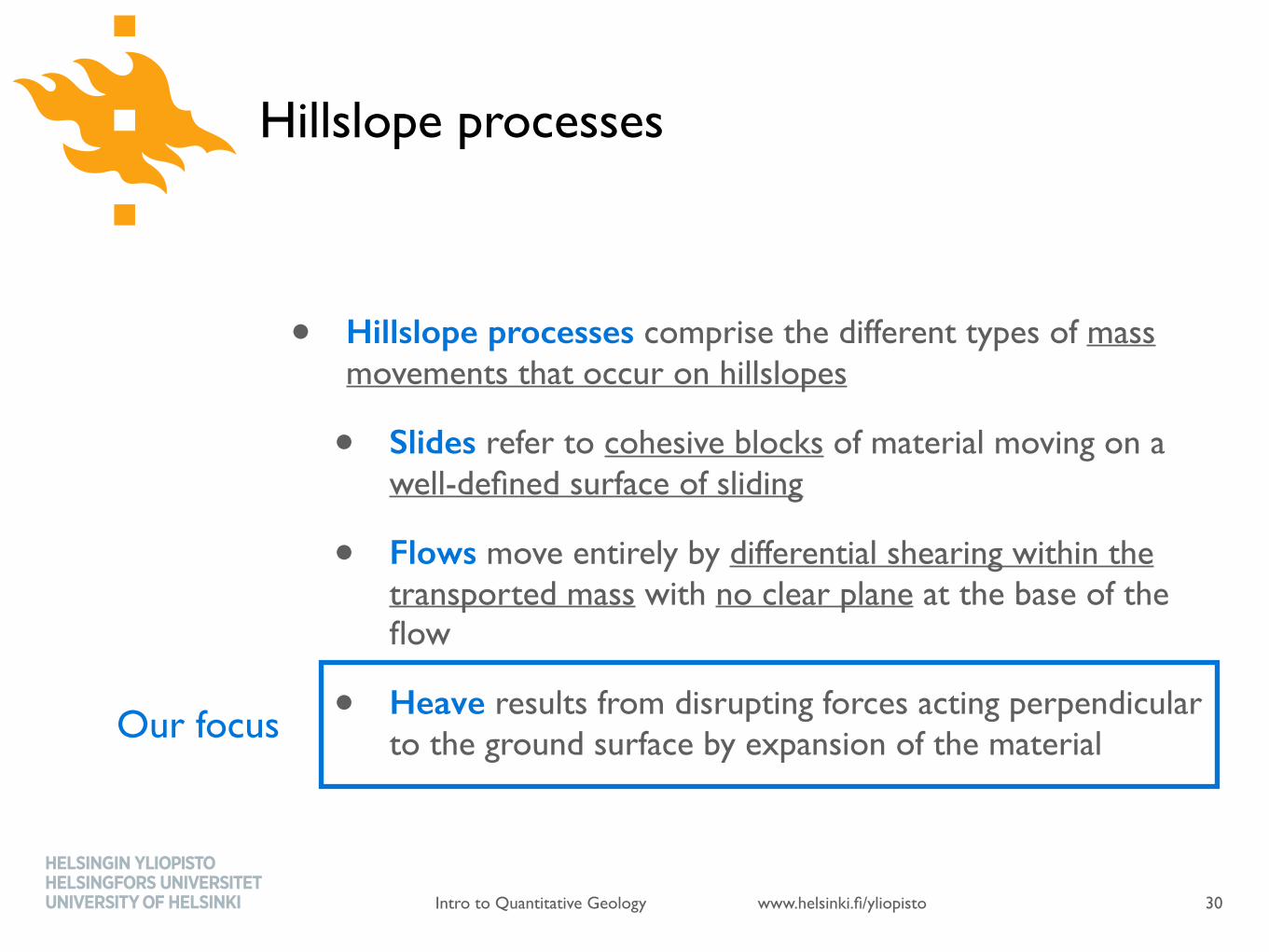
Hillslope processes
• Hillslope processes comprise the different types of mass movements that occur on hillslopes
• Slides refer to cohesive blocks of material moving on a well-defined surface of sliding
• Flows move entirely by differential shearing within the transported mass with no clear plane at the base of the flow
• Heave results from disrupting forces acting perpendicular to the ground surface by expansion of the material
30
Our focus
www.helsinki.fi/yliopistoIntro to Quantitative Geology
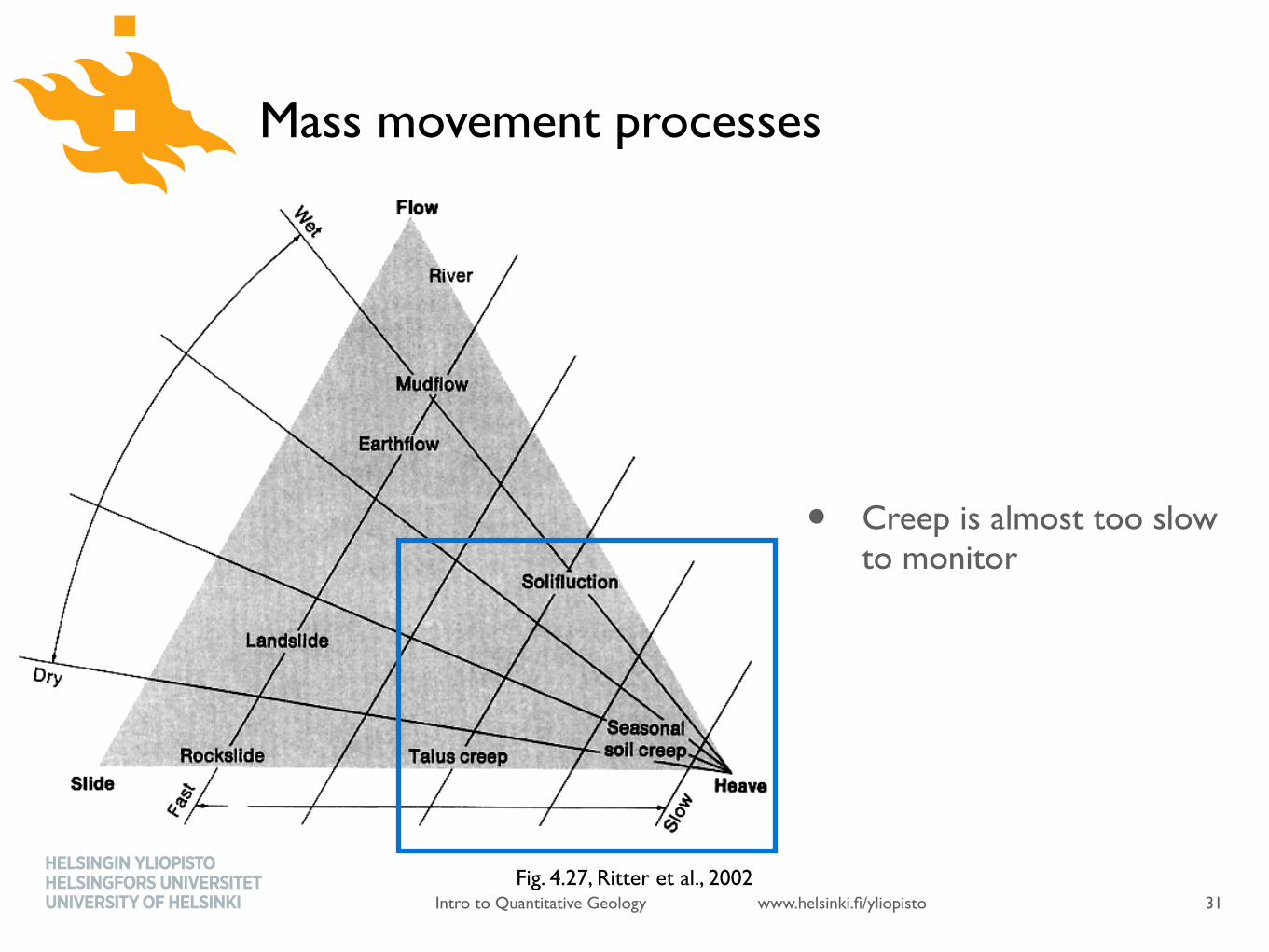
Mass movement processes
• Creep is almost too slow to monitor
31Fig. 4.27, Ritter et al., 2002
www.helsinki.fi/yliopistoIntro to Quantitative Geology
Heave and creep
• Creep: The extremely slow movement of material in response to gravity
• Heave: The vertical movement of unconsolidated particles in response to expansion and contraction, resulting in a net downslope movement on even the slightest slopes
• Seasonal creep or soil creep is periodically aided by heaving
32
www.helsinki.fi/yliopistoIntro to Quantitative Geology
Heave and creep
33
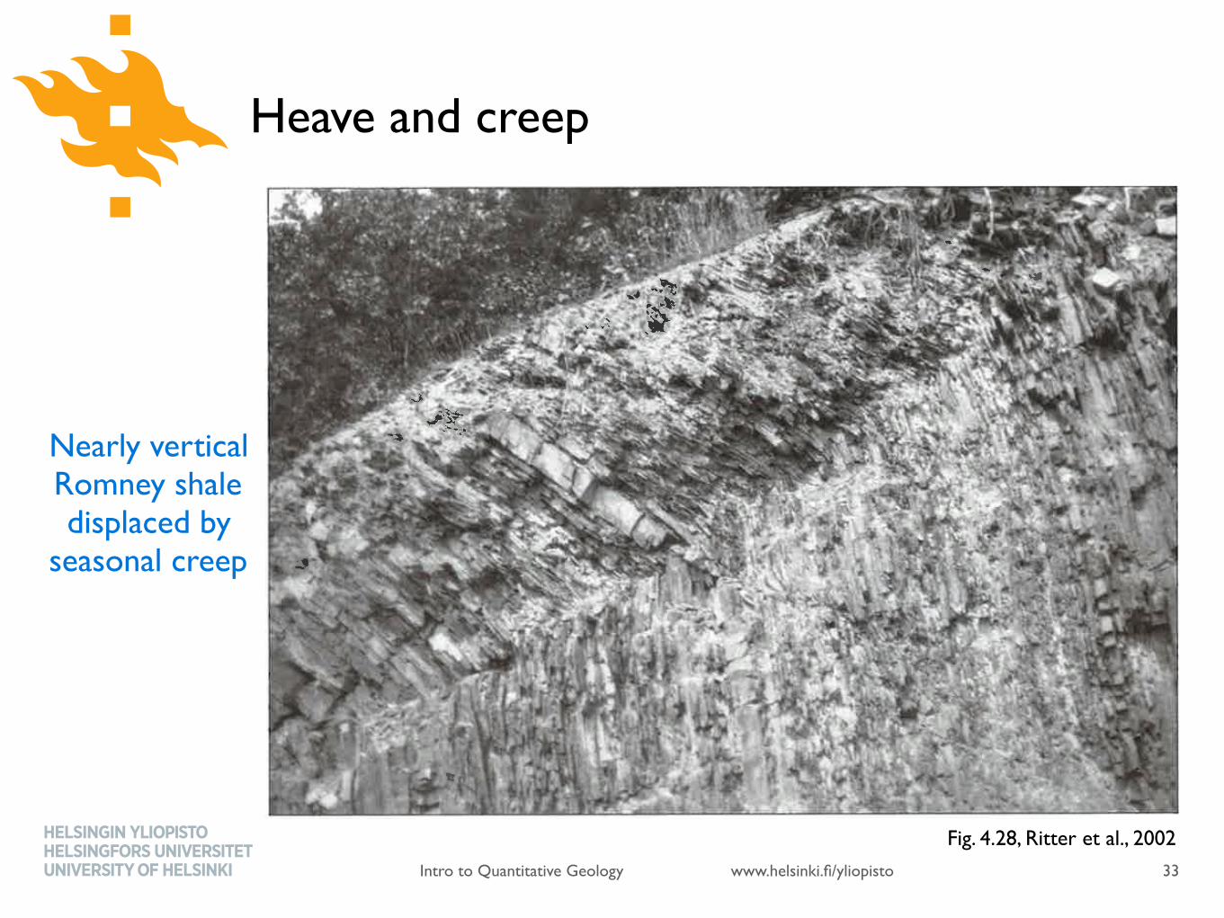
Nearly vertical Romney shale displaced by
seasonal creep
Fig. 4.28, Ritter et al., 2002
www.helsinki.fi/yliopistoIntro to Quantitative Geology
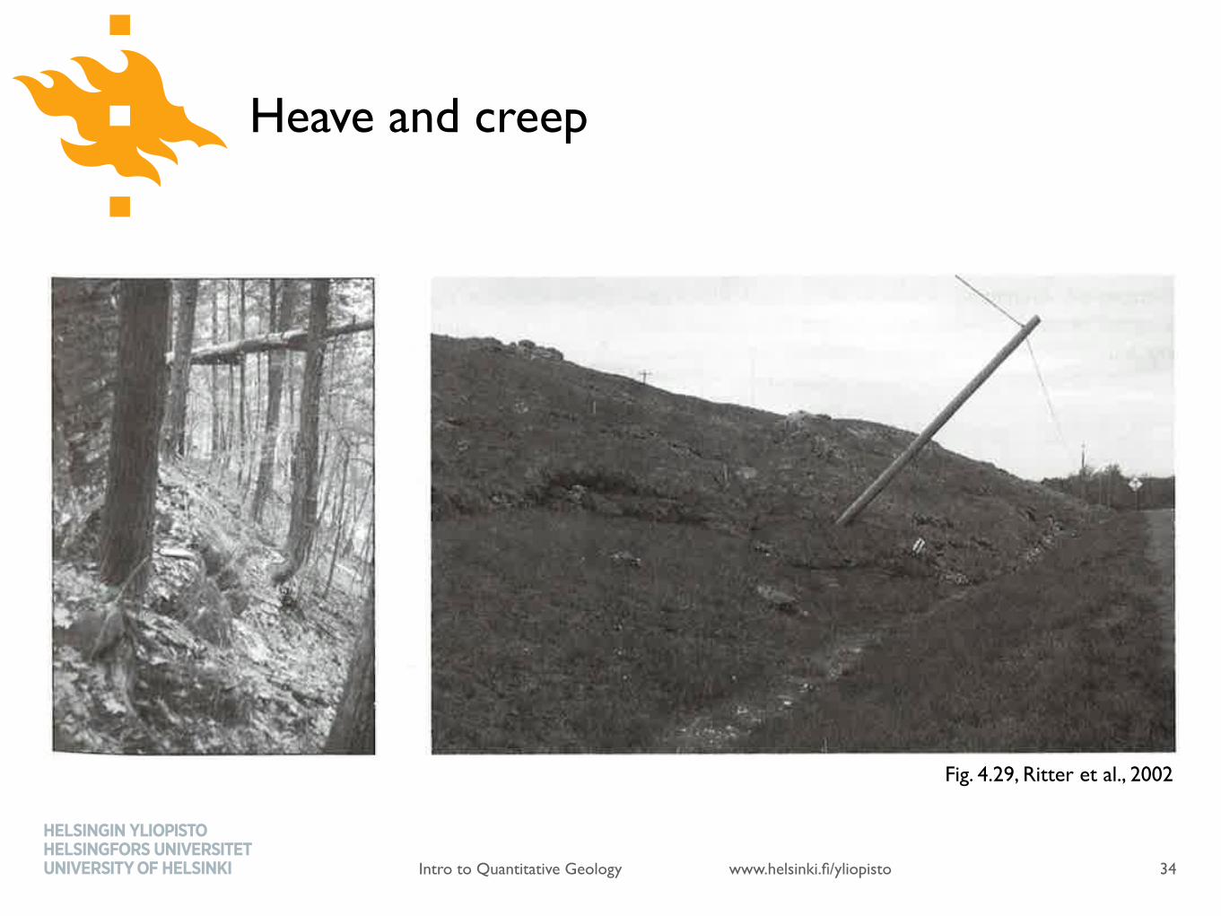
Heave and creep
34
Fig. 4.29, Ritter et al., 2002
www.helsinki.fi/yliopistoIntro to Quantitative Geology
How does heaving work?
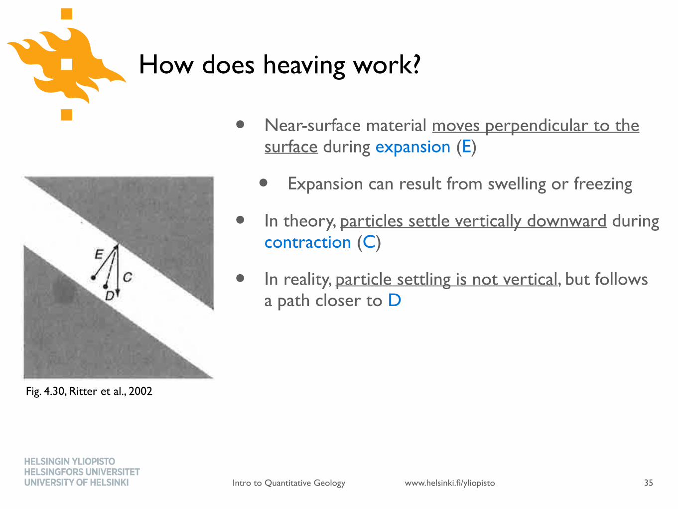
• Near-surface material moves perpendicular to the surface during expansion (E)
• Expansion can result from swelling or freezing
• In theory, particles settle vertically downward during contraction (C)
• In reality, particle settling is not vertical, but follows a path closer to D
• What influences the rate of downslope material transport by heaving?
• Slope angle, soil/regolith moisture, particle size/composition
35
Fig. 4.30, Ritter et al., 2002
www.helsinki.fi/yliopistoIntro to Quantitative Geology
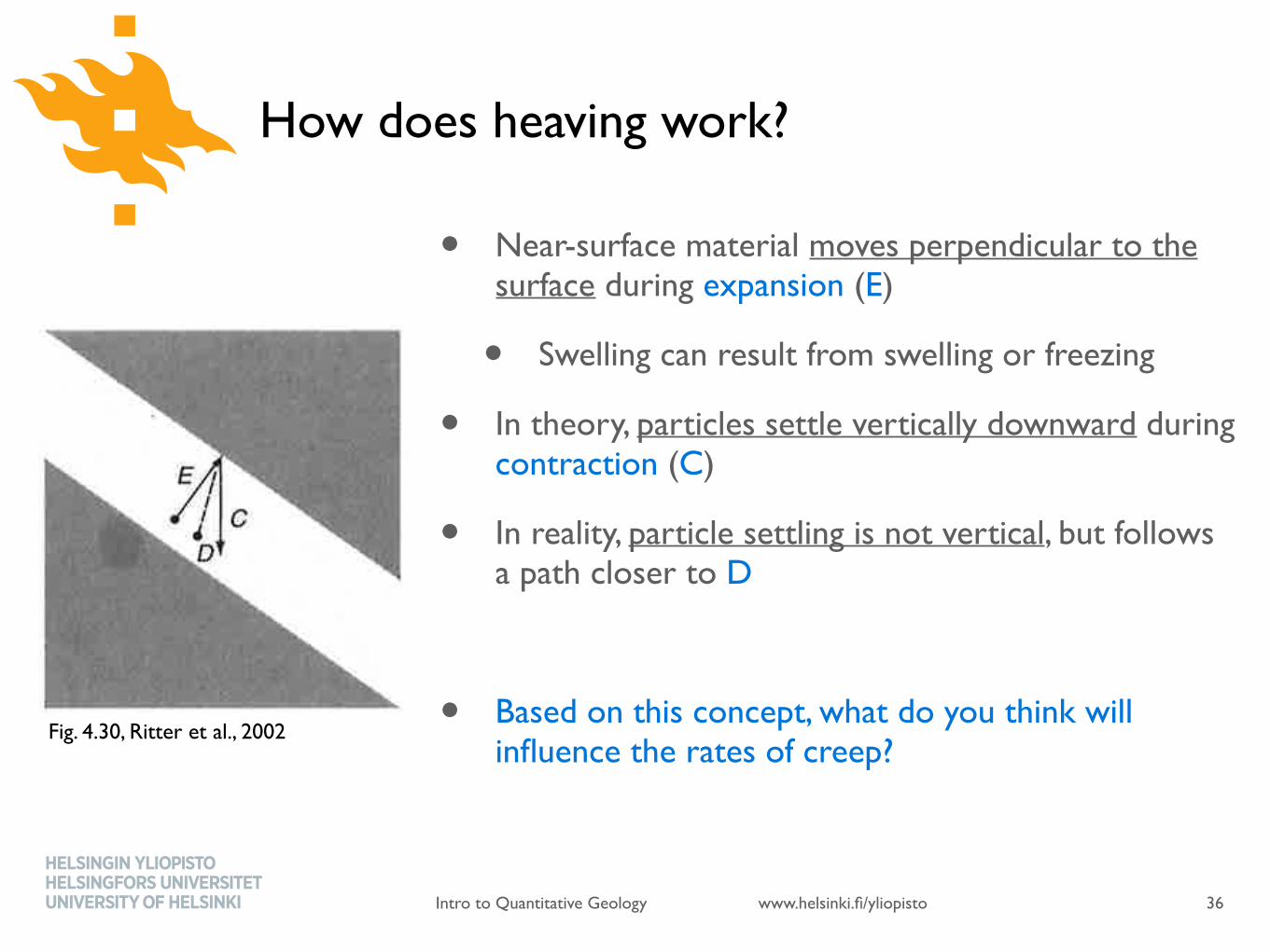
How does heaving work?
• Near-surface material moves perpendicular to the surface during expansion (E)
• Swelling can result from swelling or freezing
• In theory, particles settle vertically downward during contraction (C)
• In reality, particle settling is not vertical, but follows a path closer to D
• Based on this concept, what do you think will influence the rates of creep?
36
Fig. 4.30, Ritter et al., 2002
www.helsinki.fi/yliopistoIntro to Quantitative Geology
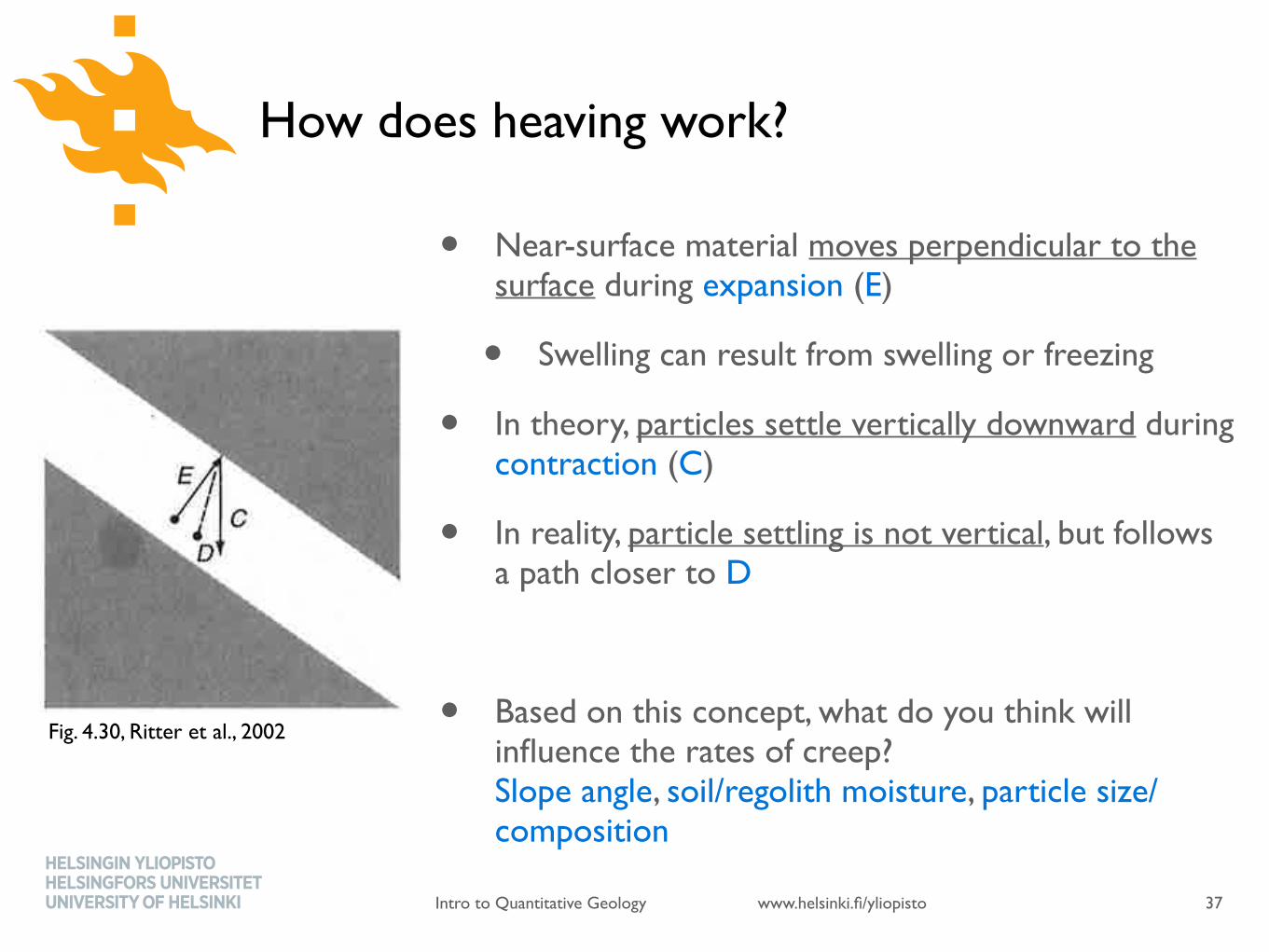
How does heaving work?
• Near-surface material moves perpendicular to the surface during expansion (E)
• Swelling can result from swelling or freezing
• In theory, particles settle vertically downward during contraction (C)
• In reality, particle settling is not vertical, but follows a path closer to D
• Based on this concept, what do you think will influence the rates of creep? Slope angle, soil/regolith moisture, particle size/composition
37
Fig. 4.30, Ritter et al., 2002
www.helsinki.fi/yliopistoIntro to Quantitative Geology
Common features of hillslope diffusion
• The rate of transport is strongly dependent on the hillslope angle
• Steeper slopes result in faster downslope transport
• In other words, the flux of mass is proportional to the topographic gradient
• This suggests these erosional processes can be modelled as diffusive
38

www.helsinki.fi/yliopistoIntro to Quantitative Geology
Recap
• What are the two components of diffusion processes?
• How does soil creep result in diffusion of soil or regolith?
• What are the main factors controlling the rate of hillslope diffusion?
39
www.helsinki.fi/yliopistoIntro to Quantitative Geology
Recap
• What are the two components of diffusion processes?
• How does soil creep result in diffusion of soil or regolith?
• What are the main factors controlling the rate of hillslope diffusion?
40
www.helsinki.fi/yliopistoIntro to Quantitative Geology
Recap
• What are the two components of diffusion processes?
• How does soil creep result in diffusion of soil or regolith?
• What are the main factors controlling the rate of hillslope diffusion?
41
www.helsinki.fi/yliopistoIntro to Quantitative Geology
Additional examples of hillslope diffusion
• Solifluction
• Rain splash
• Tree throw
• Gopher holes
42
www.helsinki.fi/yliopistoIntro to Quantitative Geology
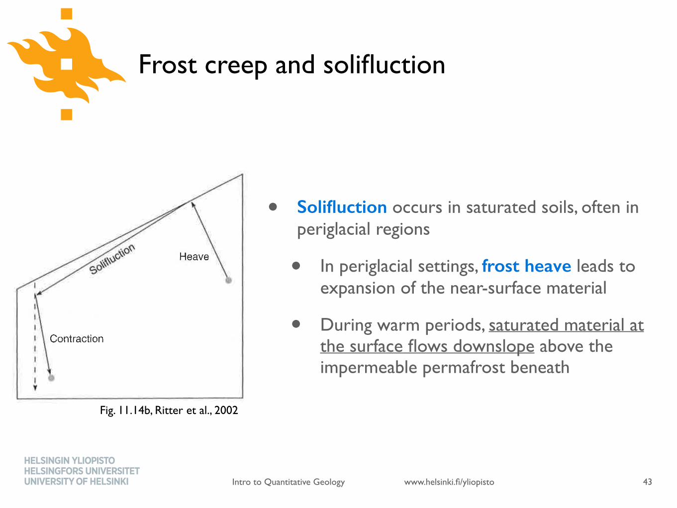
Frost creep and solifluction
• Solifluction occurs in saturated soils, often in periglacial regions
• In periglacial settings, frost heave leads to expansion of the near-surface material
• During warm periods, saturated material at the surface flows downslope above the impermeable permafrost beneath
43
Fig. 11.14b, Ritter et al., 2002
www.helsinki.fi/yliopistoIntro to Quantitative Geology
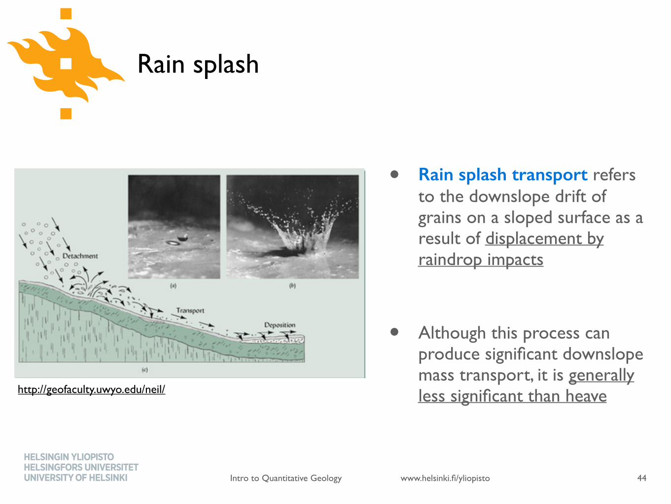
Rain splash
• Rain splash transport refers to the downslope drift of grains on a sloped surface as a result of displacement by raindrop impacts
• Although this process can produce significant downslope mass transport, it is generally less significant than heave
44
http://geofaculty.uwyo.edu/neil/
www.helsinki.fi/yliopistoIntro to Quantitative Geology
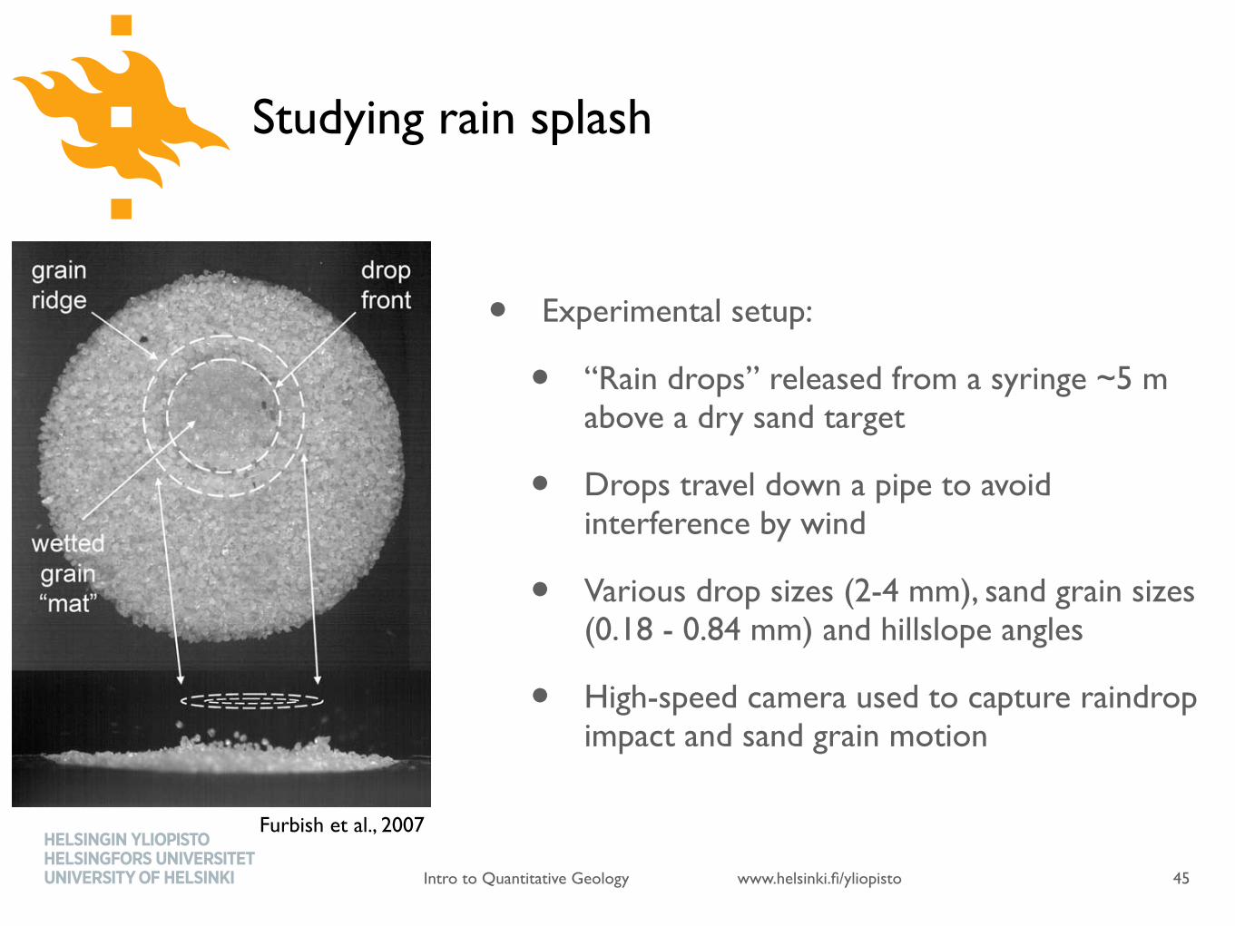
Studying rain splash
• Experimental setup:
• “Rain drops” released from a syringe ~5 m above a dry sand target
• Drops travel down a pipe to avoid interference by wind
• Various drop sizes (2-4 mm), sand grain sizes (0.18 - 0.84 mm) and hillslope angles
• High-speed camera used to capture raindrop impact and sand grain motion
45
fact, initial inward retraction of the drop (as a wetted grainmat) by surface tension starts just as grains are beinglaunched from the ridge.[19] The ejected grains have mostly low-angle trajecto-
ries. Grains entrained within the spreading fluid either donot detach from it, or are ejected as wetted clumps of grains;this is particularly noticeable with large drops on fine sand(Figure 5). With collapse of the drop such that fluid motionis largely parallel to the sediment surface, the water surfaceis essentially flush with (or lower than) the sedimentsurface. This reflects the fact that during lateral expansionthe drop entrains and transports surface grains outward fromthe center of the impact to form a small crater, as envisionedby Al-Durrah and Bradford [1982]. In addition, several ofthe videos reveal a small amount of surface dilation ‘‘far’’ahead of the advancing fluid front (over a distance that is onthe order of the radius of the impact footprint), suggestinggrain-to-grain momentum transfer beneath the visible sur-face grains.[20] The initial slope-parallel and slope-normal velocities
of ejected grains appear to be highly correlated. Grains thatare ejected from the top of the ridge (Figure 4 and Figure 6,t = 0.004 s to t = 0.010 s) have the highest initial speeds andhighest launch angles relative to the surface. Grains thatmake up the middle and bottom parts of the ridge undergosignificant grain-to-grain collisions, and thus have lowervelocities and smaller launch angles. The combination ofhigh-angle, high-velocity grains and low-angle, low-velocity grains leads to the distinctive inverted cone shapeof the raindrop grain splash (Figure 5 and Figure 6, t =0.020 s). Many more grains have low angles and lowvelocities than the relatively few high-speed grains ejectedfrom the top of the ridge.[21] For horizontal targets, ejected grain trajectories are
statistically radially symmetrical. With increasing surfaceslope, this radial symmetry is replaced with increasinglyasymmetric grain motions [Carson and Kirkby, 1972,p. 189]; at slopes approaching 30!, few upslope displace-
ments occur. Imaging reveals a clear initial asymmetry inthe speeds of the upslope and downslope parts of the grainridge, and in the slope-parallel launch speeds of grains.Surface-normal launch speeds are similar on the upslopeand downslope sides. As described below the slope-parallel
Figure 4. Image showing grains being ejected from asmall grain ridge in front of a spreading drop front atapproximately 0.004 s after initial impact; the ridge isadvancing at a rate of !25 cm s"1.
Figure 3. Plot of probability density fQ(q) with varyingconcentration factor G; downslope coincides with q = 0.
Figure 5. Image of splash from 4 mm drop on fine sandapproximately 0.02 s after initial impact, showing ejectedgrains and grain clumps.
F01001 FURBISH ET AL.: RAIN SPLASH OF DRY SAND
5 of 19
F01001
Furbish et al., 2007
www.helsinki.fi/yliopistoIntro to Quantitative Geology
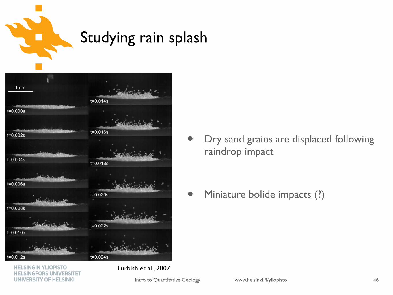
Studying rain splash
• Dry sand grains are displaced following raindrop impact
• Miniature bolide impacts (?)
46
asymmetry is manifest both in the distance that grains traveland in the numbers of grains.
4. Splash Patterns4.1. Horizontal Targets
[22] For dry conditions and horizontal targets, radialsplash distances are approximately exponentially distributedas postulated by van Dijk et al. [2002], but possibly with aheavy tail (Figure 7). The small proportion of grains landingin the 0–1 cm interval (measured from the center of impact)is partly due to censorship by the finite target size of 2 cm(thus grains landing within this interval are not accountedfor), but is also partly due to the finite size of the drop-impact footprint (up to several drop diameters) over whichgrains are accelerated (also see discussion of the data ofRiezebos and Epema [1985] by van Dijk et al. [2002]). Inaddition, the occurrence of grains in the 0–1 cm interval
(with the 2-cm target) reflects that the center of impact ofsome drops does not coincide with the target center.[23] Following van Dijk et al. [2002] and others [Wright,
1987; Mouzai and Bouhadef, 2003; Leguedois et al., 2005;Legout et al., 2005] the radial splash distance R is thusapproximately distributed as
fR rð Þ ¼ 1
m0
e$ r$r0ð Þ=m0 r % r0; ð6Þ
where r0 is an exclusion distance and m0 is the averagedistance measured beyond r0. Here, r0 may be interpreted asthe radius of the drop-impact footprint.[24] For a given sand size, splash distances are similar for
different drop sizes; the average distance may increase onlyslightly with drop size (Figure 7). The number of ejectedgrains, however, markedly increases with increasing dropsize (Figure 8). At the two extremes, 2 mm drops produce
Figure 6. Time sequence image of grains ejected from grain ridge following drop impact, showing thatgrains ejected from top of ridge have highest initial speeds and launch angles, whereas grains that makeup the middle and bottom part of ridge have lower initial speeds and launch angles following grain-to-grain collisions; note initial corona-like splash of water (t = 0.002 s) preceding significant grain motion.
F01001 FURBISH ET AL.: RAIN SPLASH OF DRY SAND
6 of 19
F01001
Furbish et al., 2007
www.helsinki.fi/yliopistoIntro to Quantitative Geology
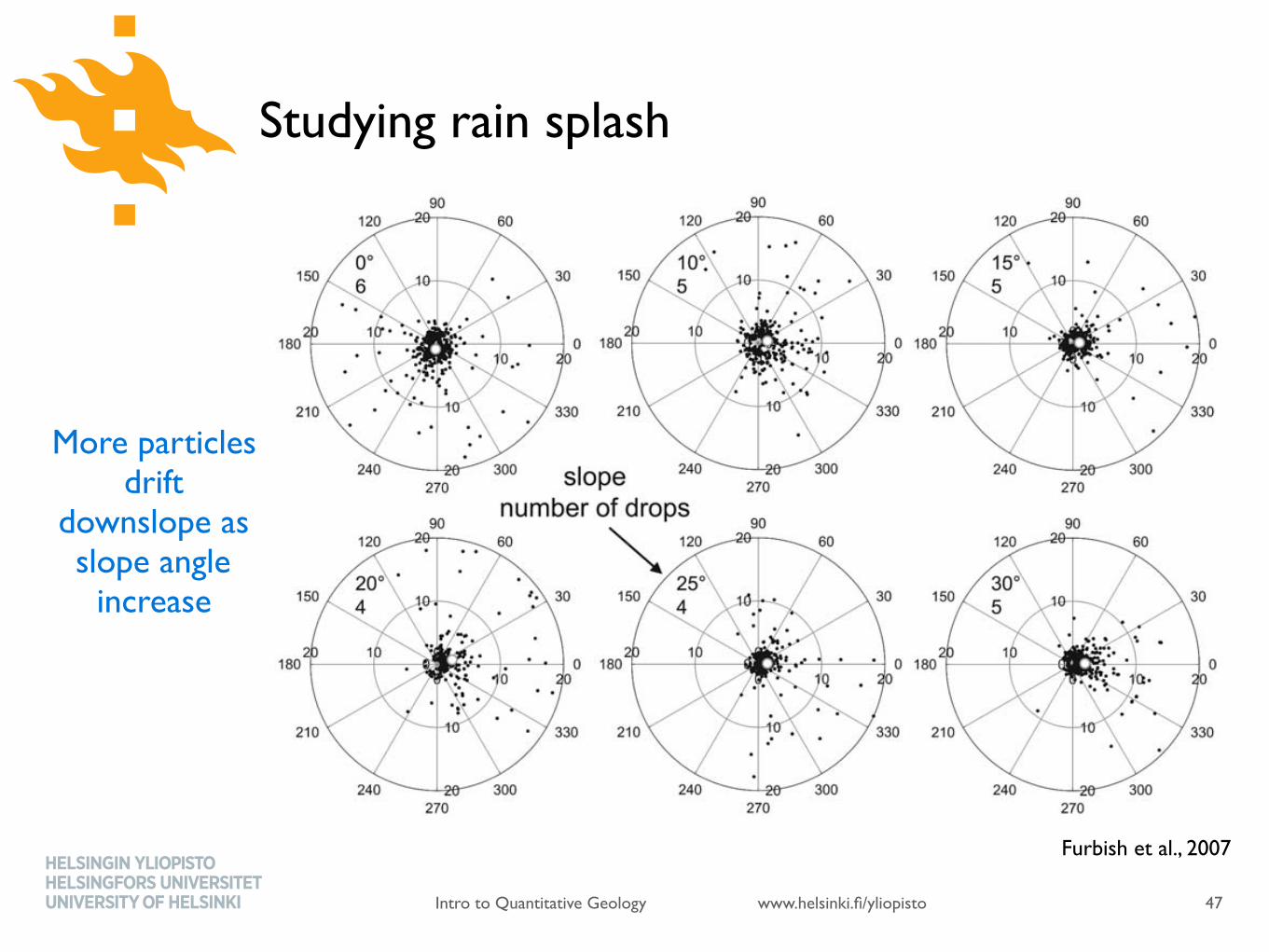
Studying rain splash
47
with m0 = 2 cm and Kb ! 1.74, the coefficient K ! 0.0001cm"2 s"1.[34] Effects of raindrop properties (intensity, size distri-
bution, kinetic energy) are examined further separately. Wereemphasize that the work here is limited to dry sandconditions. Moreover, our experiments with sticky papertargets exclude the possibility that splashed grains mightbounce upon landing, an effect we observed in experimentswithout sticky paper. We expect that such bouncing wouldincrease average displacements, particularly with increasingslope.
6. Discussion and Conclusions
[35] It is well appreciated that grain detachment andsplash generally increase with drop size in relation to dropmomentum or kinetic energy. Nonetheless there is continu-ing debate regarding the relative performance of these andother quantities (for example, drop pressure and rain inten-sity) in predicting detachment [Salles et al., 2001]. Inseminal work on this topic, Sharma and Gupta [1989]and Sharma et al. [1991] plot and statistically fit detachedgrain mass versus both momentum and kinetic energy. Theynote that the fits (and R2 values) are similar, and then state:‘‘Since KE is predominantly used as an erosivity parameterin raindrop erosion modeling, our discussion henceforthwill only consider KE-based relationships’’ [Sharma et al.,1991, p. 305]. Indeed, the plots of detached grain massversus momentum and grain mass versus kinetic energy forthe loamy sand to clay soils reported by Sharma et al.[1991] suggest that linear fits between detached mass andmomentum (involving a threshold momentum value) are at
least as good, if not better, than fits between detached massand kinetic energy. Salles et al. [2001] point out thatexperimental splash data typically are not sufficiently pre-cise to distinguish between these alternatives, and reportthat for both sand and silt loam, linear fits between detachedgrain mass and drop momentum, and between grain massand kinetic energy, are not statistically different. Likewise,our data do not suggest a significant difference in linear fitsbetween detached grain mass and momentum (Figure 10)and between grain mass and kinetic energy (not plotted),likely because the data span an insufficient range in dropmomentum (or kinetic energy). Indeed, a simple scalinganalysis (Appendix C) suggests that such plots ought to benonlinear, as the slope of the physical relationship betweenejected grain mass and either momentum or kinetic energyimplicitly contains a characteristic (unmeasured) grainspeed that varies with momentum or kinetic energy.[36] Within this context, our imaging of drops landing on
targets of different sizes of sand and on a high-permeabilityporous stone suggests that initial infiltration during impact[Mihara,1952] modulates the relation between the mass ofdetached grains and drop size. Namely, for small drop-to-grain size ratio R0 = D/d, significant infiltration can occurduring impact due to the high dynamic pressure thatmomentarily exists during the small time interval t # D/W(Table 2), such that the drop mass involved in lateralspreading is smaller than would otherwise occur. With largeR0, the permeability of the sand limits infiltration during tand proportionally more drop mass accelerates laterally.Inasmuch as the lateral momentum of the spreading dropis responsible for grain ejection, then the improved linearrelation between the ejected grain mass and the momentum
Figure 11. Radial plots of final ejected grain positions showing increasing asymmetry with increasingslope, with mass centroids (white circles). Radial distances are in cm.
F01001 FURBISH ET AL.: RAIN SPLASH OF DRY SAND
10 of 19
F01001
Furbish et al., 2007
More particles drift
downslope as slope angle
increase
www.helsinki.fi/yliopistoIntro to Quantitative Geology
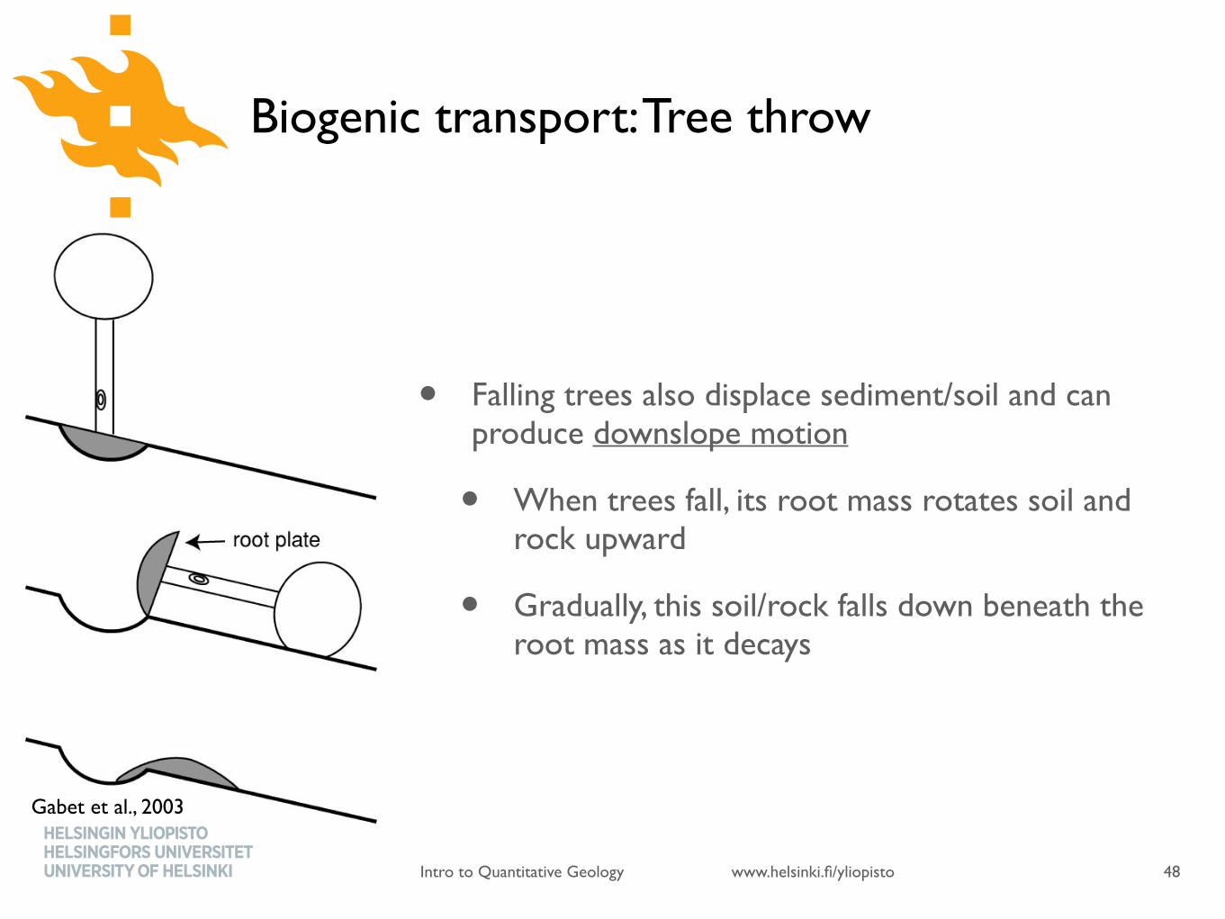
Biogenic transport: Tree throw
• Falling trees also displace sediment/soil and can produce downslope motion
• When trees fall, its root mass rotates soil and rock upward
• Gradually, this soil/rock falls down beneath the root mass as it decays
48
6 Mar 2003 22:16 AR AR182-EA31-07.tex AR182-EA31-07.SGM LaTeX2e(2002/01/18) P1: FHD
256 GABET ⌅ REICHMAN ⌅ SEABLOOM
Tree Throw
SEDIMENT TRANSPORT A tree is uprooted when the lateral forces on the crownand trunk exceed the ability of the roots and soil to hold it in place (Putz et al.1983). Strong winds are often responsible for toppling trees (e.g., Kotarba 1970),although other causes may include overloading by snow, root decay of dead trees,and being knocked down by other falling trees [these are reviewed by Schaetzl et al.(1989)]. When a tree is uprooted and falls over, the root mass that binds soil androck is rotated up, leaving a pit (Figure 3). As the roots’ grip on the soil weakens
Figure 3 Illustration of the creation of pit and moundtopography when a tree topples over.
Ann
u. R
ev. E
arth
Pla
net.
Sci.
2003
.31:
249-
273.
Dow
nloa
ded
from
ww
w.a
nnua
lrevi
ews.o
rgby
Hel
sink
i Uni
vers
ity o
n 03
/23/
14. F
or p
erso
nal u
se o
nly.
Gabet et al., 2003
www.helsinki.fi/yliopistoIntro to Quantitative Geology
Biogenic transport: Gopher holes
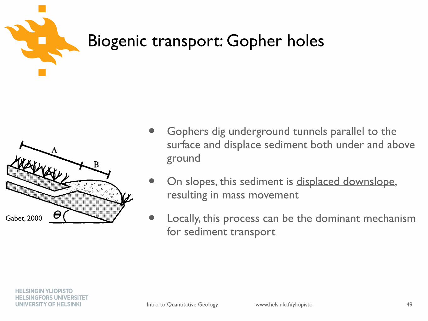
• Gophers dig underground tunnels parallel to the surface and displace sediment both under and above ground
• On slopes, this sediment is displaced downslope, resulting in mass movement
• Locally, this process can be the dominant mechanism for sediment transport
49
a surface path (B). Section A is the transport distance from within the burrow to the burrow opening and isdetermined by calculating the length of tunnel necessary to produce the volume of soil in the mound. Thisassumes that the soil in the mound is derived from the proximal portion of the associated tunnel and is,therefore, a minimum transport distance. A! is the x-component of the net downslope transport from the tunnelcentroid to the burrow entrance:
A! " A cos! cos " #4$
where the burrowing angle, !, is the angle between%Z (the direction of steepest slope) and the tunnel (Figure2), and " is the hillslope gradient. This presupposes that !, which is a function of burrowing strategy, variesaccording to hillslope gradient. This is reasonable considering that pushing soil uphill, downhill or along acontour will have different bioenergetic costs (Vleck, 1981).Section B is the distance from the burrow entrance to the visually estimated mound centroid. B! is the
x-component of the downhill transport:
B! " B cos " #5$
The total x-component of the downslope transport distance is then equal to the sum of A! and B!. The general
Figure 1. Profile view of gopher tunnel and mound illustrating the sediment transport path. A is the distance from the centroid of thetunnel to the burrow opening, B is the distance from the burrow opening to the mound centroid, and " is the hillslope gradient. Thetunnel is partially backfilled by displaced soil, indicating that this mound is ‘terminal.’ Note that the tunnel is parallel to the ground
surface
Figure 2. Planform view of gopher tunnel and mound illustrating the effect of burrowing angle, !, on the downslope subsurfacetransport distance. For example, there is no net downslope subsurface transport if ! is 90 °
Copyright ! 2000 John Wiley & Sons, Ltd. Earth Surf. Process. Landforms 25, 1419–1428 (2000)
GOPHER BIOTURBATION 1421
Gabet, 2000
www.helsinki.fi/yliopistoIntro to Quantitative Geology
References
Furbish, D. J., Hamner, K. K., Schmeeckle, M., Borosund, M. N., & Mudd, S. M. (2007). Rain splash of dry sand revealed by high-speed imaging and sticky paper splash targets. J. Geophys. Res., 112(F1), F01001. doi:10.1029/2006JF000498
Gabet, E. J. (2000). Gopher bioturbation: Field evidence for non-linear hillslope diffusion. Earth Surface Processes and Landforms, 25(13), 1419–1428.
Gabet, E. J., Reichman, O. J., & Seabloom, E. W. (2003). THE EFFECTS OF BIOTURBATION ON SOIL PROCESSES AND SEDIMENT TRANSPORT. Annual Review of Earth and Planetary Sciences, 31(1), 249–273. doi:10.1146/annurev.earth.31.100901.141314
Ritter, D. F., Kochel, R. C., & Miller, J. R. (2002). Process Geomorphology (4 ed.). MgGraw-Hill Higher Education.
Shuster, D. L., Flowers, R. M., & Farley, K. A. (2006). The influence of natural radiation damage on helium diffusion kinetics in apatite. Earth and Planetary Science Letters, 249(3-4), 148–161.
50