natural deduction, hybrid systems and modal logics || standard approach to basic modal logics
TRANSCRIPT
Chapter 6
Standard Approach to BasicModal Logics
In this Chapter we focus on the class of non-axiomatic systems that arecalled standard in the sense of keeping intact all the machinery of suitablesystems for classical logic. Extensions are obtained by means of additionalmodal rules. This group covers modal extensions of standard Gentzen SC,Hintikka-style modal TS,1 and some ND systems.
No doubt systems of this sort are the earliest and the most popularnon-axiomatic formalizations of modal logics in general. In this Chapter werestrict a presentation to formalizations of basic logics because most of theproposals are limited only to some logics in this family. Moreover, thereis a straightforward correspondence of results between SC, TS and ND instandard approaches as far as they are stated as formalizations of basiclogics, so they make a really uniform group. As we shall see in the nextChapter, this correspondence is sometimes broken when we left a family ofbasic logics.
Close resemblance of SC’s and TS’s of this type does not require explana-tion; in Chapter 3 we already explained that the latter is just an inversionand simplification of the former in classical logic, and it is true also formodal extensions. In what way standard ND-systems are related to thesesystems will be explained in what follows. For the time being we point outonly one thing; a characteristic property of all these systems is that rulesfor modal operators lead to the loss of some information and/or modifica-tion of the rest. In SC and TS it is connected with putting side-conditions
1We mean the family of TS’s called implicit by Gore [117].
A. Indrzejczak, Natural Deduction, Hybrid Systems and Modal Logics, 182Trends in Logic 30, DOI 10.1007/978-90-481-8785-0 6,c© Springer Science+Business Media B.V. 2010
6.1. STANDARD SEQUENT CALCULI 183
on parametric formulae. In the most popular modal ND it is connectedwith the introduction of a special category of subproofs, where reiterationof formulae is limited.2
It seems reasonable to start with short presentation of standard SCsystems for basic modal logic first, in Section 6.1. They may be seen as aneasy point of reference, and in fact, they were historically the first formsof non-axiomatic formalizations of modal logics. Standard TS’s are notdiscussed separately but collected together with SC’s.
In case of ND we have a division of ways. There are four basic approachesto modality via ND-formalization which may be called standard since theydo not alter radically the basic format of ND system for classical logic.They are based on: modalization of assumptions, modalization of rules,modalization of reiteration rule, application of modal assumptions. In fact,the last two may be seen as language-based variants of basically the samemethods: Fitch’s technique of modal (or strict) subderivations, where theformer deals rather with �, whereas the latter is based on ♦. In manyversions, including Fitch original work, these two approaches are indeedmixed together. They are separated by some authors, e.g. Fitting [93],because of semantic reasons; we will show one more difference, of syntacticcharacter. In Sections 6.2, 6.3, and 6.4. we present all these approachesto modal ND, paying attention to practical matters, especially the scopeof applicability. As a result only Fitch’s approach seems to be reasonablyextensive. The last two sections show how Fitch’s approach to ND may beextended to weak modal logics, and to first-order modal logics.
6.1 Standard Sequent Calculi and Tableau Sys-tems
6.1.1 Historical Remarks
It seems that extensions of standard SC to some modal logics were evenearlier than invention of full-fledged semantics, since they were prior tofamous works of Kripke [169], Hintikka [132] and others. The first modalsequent systems appeared in Feys [85] (for S4), Curry [75, 76] (for S4 andS5), Ridder [233] (also T) and Kanger [160] (the same logics). However themost fundamental work in this field was due to Ohnishi and Matsumoto [197,198], where some weaker logics like S2 and S3 were also formalized. This
2In fact, also a system of destructive resolution of [94] may be included in this group –it will be introduced later in Chapter 7 (Section 7.4.2).
184 CHAPTER 6. STANDARD APPROACH TO MODAL LOGICS
line of investigation was then extended by Zeman [288] and Fitting [93] tomany normal and regular logics.3 In variety of later works this approach wasextended to many other regular and normal logics including such importantones like G and S4Grz. Some of these extensions of standard SC will bedescribed later in Chapter 7 and 9. More detailed historical remarks maybe found e.g. in [93, 116, 280, 281]. SC systems for logics weaker thanregular were introduced much later by Lavendhomme and Lucas [172], andby Indrzejczak [152, 154].
Although the first tableau formalizations of some modal logics due toKripke were invented in late 50s we will not treat them as standard, anda discussion of them will be postponed to Chapter 7 because of reasonswhich will be explained therein. Tableau systems which are called standardin this book were devised much later. These are TS’s in Hintikka format,introduced by Rautenberg [229] and extended by others (cf. Gore [116, 117]for detailed documentation) to variety of other normal logics.
6.1.2 Standard SC for Basic Modal Logics
As we mentioned above, standard modal SC is obtained just by addition ofextra rules for modals to Gentzen SC for CPL. For example, to obtain aformalization of K in a language with box only (i.e. L�), it is sufficient toadd only one rule:
(⇒ �) Γ ⇒ ϕ�Γ ⇒ �ϕ
In case of a language with ♦ we need additionally the following rule:
(♦ ⇒) ϕ⇒ Δ♦ϕ⇒ ♦Δ
It is worth remarking that although addition of any of these rules to SCfor CPL provides an adequate formalization of K in a language with onemodal constant, the addition of both rules is not sufficient for completenessof K in full LM. It was already noted by Kripke [170] that such rules areinsufficient for proving interdefinability of � and ♦. In order to remedy theproblem one should rather use the following pair of rules:
(⇒ �′) Γ ⇒ Δ, ϕ�Γ ⇒ ♦Δ,�ϕ (♦ ⇒′) ϕ,Γ ⇒ Δ
♦ϕ,�Γ ⇒ ♦Δ
3In fact Zeman’s work contains formalizations of the whole Lewis’ family S1–S5.
6.1. STANDARD SEQUENT CALCULI 185
The modification of these rules and the addition of others leads to for-malization of many normal logics. In particular, to obtain T it is enoughto add to the formalization of K the following pair of rules:
(� ⇒) ϕ,Γ ⇒ Δ�ϕ,Γ ⇒ Δ (⇒ ♦) Γ ⇒ Δ, ϕ
Γ ⇒ Δ,♦ϕ
The formalization of other logics, e.g. transitive, requires usually atleast a modification of rules (⇒ �′) and (♦ ⇒′), taking into account a typeof operations admissible on parametric formulae. For example, in order toget SC for S4, we add to CPL (⇒ ♦), (� ⇒) and the following variants of(♦ ⇒′) and (⇒ �′):
(⇒ �4) �Γ ⇒ ♦Δ, ϕ�Γ ⇒ ♦Δ,�ϕ (♦ ⇒4) ϕ,�Γ ⇒ ♦Δ
♦ϕ,�Γ ⇒ ♦Δ
Since, at least for basic logics, such an approach requires only a suitablemodification of rules (♦ ⇒′) and (⇒ �′), it may be nicely summarized inthe general schemata due to Fitting:
(⇒ �F ) Γ� ⇒ Δ�, ϕΓ ⇒ Δ,�ϕ (♦ ⇒F ) ϕ,Γ� ⇒ Δ�
♦ϕ,Γ ⇒ Δ
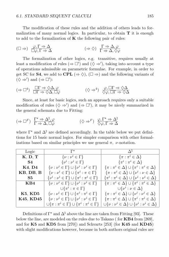
where Γ� and Δ� are defined accordingly. In the table below we put defini-tions for 15 basic normal logics. For simpler comparison with other formal-izations based on similar principles we use general π, ν-notation.
Logic Γ� Δ�
K, D, T {ν : νi ∈ Γ} {π : πi ∈ Δ}S4 {νi : νi ∈ Γ} {πi : πi ∈ Δ}
K4, D4 {ν : νi ∈ Γ} ∪ {νi : νi ∈ Γ} {π : πi ∈ Δ} ∪ {πi : πi ∈ Δ}KB, DB, B {ν : νi ∈ Γ} ∪ {πi : π ∈ Γ} {π : πi ∈ Δ} ∪ {νi : ν ∈ Δ}
S5 {νi : νi ∈ Γ} ∪ {πi : πi ∈ Γ} {πi : πi ∈ Δ} ∪ {νi : νi ∈ Δ}KB4 {ν : νi ∈ Γ} ∪ {νi : νi ∈ Γ} {π : πi ∈ Δ} ∪ {πi : πi ∈ Δ}
∪{πi : π ∈ Γ} ∪{νi : ν ∈ Δ}K5, KD5 {ν : νi ∈ Γ} ∪ {πi : πi ∈ Γ} {π : πi ∈ Δ} ∪ {νi : νi ∈ Δ}
K45, KD45 {ν : νi ∈ Γ} ∪ {νi : νi ∈ Γ} {π : πi ∈ Δ} ∪ {πi : πi ∈ Δ}∪{π : πi ∈ Γ} ∪ {πi : πi ∈ Γ} ∪{ν : νi ∈ Δ} ∪ {νi : νi ∈ Δ}
Definitions of Γ� and Δ� above the line are taken from Fitting [93]. Thesebelow the line, are modeled on the rules due to Takano ( for KB4 from [269],and for K5 and KD5 from [270]) and Schvarts [253] (for K45 and KD45)with slight modifications however, because in both authors original rules are
186 CHAPTER 6. STANDARD APPROACH TO MODAL LOGICS
defined in L�. In some cases it is possible to simplify the definition, but wewill illustrate this later when discussing ND system based on the use of thereiteration rule.
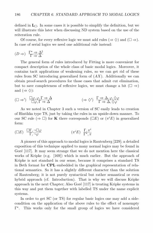
Of course, for every reflexive logic we must add rules (⇒ ♦) and (� ⇒).In case of serial logics we need one additional rule instead:
(D ⇒) Γ� ⇒ Δ�
Γ ⇒ Δ
The general form of rules introduced by Fitting is more convenient forcompact description of the whole class of basic modal logics. Moreover, itcontains tacit applications of weakening rules, so we can get rid of theserules from SC introducing generalized form of (AX). Additionally we canobtain proof-search procedures for those cases that admit cut elimination,but to save completeness of reflexive logics, we must change a bit (� ⇒)and (⇒ ♦):
(� ⇒′) �ϕ,ϕ,Γ ⇒ Δ�ϕ,Γ ⇒ Δ (⇒ ♦′) Γ ⇒ Δ, ϕ,♦ϕ
Γ ⇒ Δ,♦ϕ
As we noted in Chapter 3 such a version of SC easily leads to creationof Hintikka type TS, just by taking the rules in an upside-down manner. Toour SC rule (⇒ �) for K there corresponds (�E) or (πiE) in generalizedform:
(�E) �Γ,¬�ϕΓ,¬ϕ (πiE) Γ, πi
Γ�, π
A pioneer of this approach to modal logics is Rautenberg [229]; a detailedexposition of this technique applied to many normal logics may be found inGore [117]. It may seem strange that we do not mention here the classicalworks of Kripke (e.g. [169]) which is much earlier. But the approach ofKripke is not standard in our sense, because it comprises a standard TSin Beth format for CPL embedded in the graphical representation of rela-tional semantics. So it has a slightly different character than the solutionof Rautenberg; it is not purely syntactical but rather semantical or evenhybrid approach (cf. Introduction). That is why we will discuss Kripkeapproach in the next Chapter; Also Gore [117] is treating Kripke systems inthis way and put them together with labelled TS under the name explicitsystems.
In order to get SC (or TS) for regular basic logics one may add a side-condition on the application of the above rules to the effect of nonempty�. This works only for the small group of logics we have considered
6.1. STANDARD SEQUENT CALCULI 187
in Chapter 5; some other regular (and quasi-regular) logics need furthermodifications described in [93].
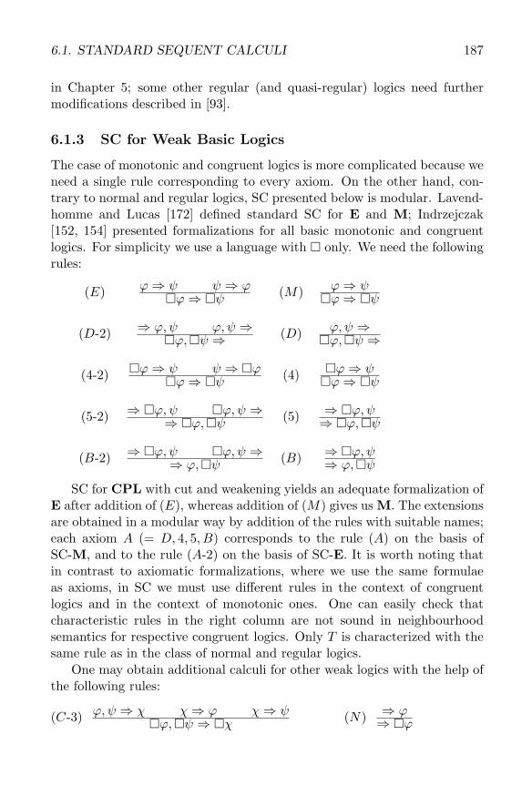
6.1.3 SC for Weak Basic Logics
The case of monotonic and congruent logics is more complicated because weneed a single rule corresponding to every axiom. On the other hand, con-trary to normal and regular logics, SC presented below is modular. Lavend-homme and Lucas [172] defined standard SC for E and M; Indrzejczak[152, 154] presented formalizations for all basic monotonic and congruentlogics. For simplicity we use a language with � only. We need the followingrules:
(E) ϕ⇒ ψ ψ ⇒ ϕ�ϕ⇒ �ψ (M) ϕ⇒ ψ
�ϕ⇒ �ψ
(D-2) ⇒ ϕ,ψ ϕ, ψ ⇒�ϕ,�ψ ⇒ (D) ϕ,ψ ⇒
�ϕ,�ψ ⇒
(4-2) �ϕ⇒ ψ ψ ⇒ �ϕ�ϕ⇒ �ψ (4) �ϕ⇒ ψ
�ϕ⇒ �ψ
(5-2) ⇒ �ϕ,ψ �ϕ,ψ ⇒⇒ �ϕ,�ψ (5) ⇒ �ϕ,ψ
⇒ �ϕ,�ψ
(B-2) ⇒ �ϕ,ψ �ϕ,ψ ⇒⇒ ϕ,�ψ (B) ⇒ �ϕ,ψ
⇒ ϕ,�ψ
SC for CPL with cut and weakening yields an adequate formalization ofE after addition of (E), whereas addition of (M) gives us M. The extensionsare obtained in a modular way by addition of the rules with suitable names;each axiom A (= D, 4, 5, B) corresponds to the rule (A) on the basis ofSC-M, and to the rule (A-2) on the basis of SC-E. It is worth noting thatin contrast to axiomatic formalizations, where we use the same formulaeas axioms, in SC we must use different rules in the context of congruentlogics and in the context of monotonic ones. One can easily check thatcharacteristic rules in the right column are not sound in neighbourhoodsemantics for respective congruent logics. Only T is characterized with thesame rule as in the class of normal and regular logics.
One may obtain additional calculi for other weak logics with the help ofthe following rules:
(C-3) ϕ,ψ ⇒ χ χ⇒ ϕ χ⇒ ψ�ϕ,�ψ ⇒ �χ (N) ⇒ ϕ
⇒ �ϕ
188 CHAPTER 6. STANDARD APPROACH TO MODAL LOGICS
(N) is simply a sequent formulation of (RG) which allows us to getformalizations of EN-logics and MN-logics mentioned in the last Chapter.(C-3) corresponds to axiom C: �ϕ∧�ψ → �(ϕ∧ψ) on the ground of E; itenables a formalization of the class of EC-logics. The addition of this ruleto calculi for monotonic logics does not make sense since they collapse intoregular ones (K is derivable). In fact, to change SC-M into SC-R we needmuch simpler rule (C): ϕ,ψ ⇒ χ / �ϕ,�ψ ⇒ �χ which cannot be usedfor congruent logics because it is not sound in EC.
6.2 Some Standard ND for Modal Basic Logics
In contrast to the situation in SC and TS, we may distinguish more than oneND formalization for modal logics which may be called standard (since thebasic ND system for CPL is not modified). There are four such approachesto modality via ND-formalization, based on: modalization of assumptions,modalization of rules, modalization of reiteration rule, application of modalassumptions. In fact, the last two approaches may be seen as language-based variants of basically the one method: Fitch’s technique of modal (orstrict) subderivations.
The first two approaches rather fail to be extensive, hence they aretreated briefly in one section in contrast to the last two that have quite asatisfying scope of application and will be discussed thoroughly.
6.2.1 Modal Assumptions
The first approach to the extension of ND-techniques to modal logics, dueto Curry [75], was based on the concept of modal assumptions. The idea isthat the application of some rule of necessity introduction to a formula ϕis dependent on the shape of undischarged assumptions of ϕ. It should belimited to cases where the set of assumptions is empty or consists only ofsomewhat modalized assumptions. In the first case it is simply an applica-tion of (RG), in the second, we must check all the assumptions whether theysatisfy suitable conditions defined for respective logic. Curry [75] definedhis system only for propositional S4 but this approach was soon, and ratherindependently, extended by others. Borkowski and S�lupecki [54] provide asystem for S4 and S5 but in the language with strict implication as prim-itive. Prawitz [220] formalized the same modal logics but also on minimaland intuitionistic basis and in first-order language. A similar system for S5was provided by Corcoran [74].
6.2. SOME STANDARD ND FOR MODAL BASIC LOGICS 189
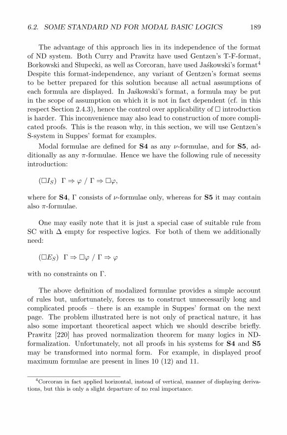
The advantage of this approach lies in its independence of the formatof ND system. Both Curry and Prawitz have used Gentzen’s T-F-format,Borkowski and S�lupecki, as well as Corcoran, have used Jaskowski’s format4
Despite this format-independence, any variant of Gentzen’s format seemsto be better prepared for this solution because all actual assumptions ofeach formula are displayed. In Jaskowski’s format, a formula may be putin the scope of assumption on which it is not in fact dependent (cf. in thisrespect Section 2.4.3), hence the control over applicability of � introductionis harder. This inconvenience may also lead to construction of more compli-cated proofs. This is the reason why, in this section, we will use Gentzen’sS-system in Suppes’ format for examples.
Modal formulae are defined for S4 as any ν-formulae, and for S5, ad-ditionally as any π-formulae. Hence we have the following rule of necessityintroduction:
(�IS) Γ ⇒ ϕ / Γ ⇒ �ϕ,
where for S4, Γ consists of ν-formulae only, whereas for S5 it may containalso π-formulae.
One may easily note that it is just a special case of suitable rule fromSC with Δ empty for respective logics. For both of them we additionallyneed:
(�ES) Γ ⇒ �ϕ / Γ ⇒ ϕ
with no constraints on Γ.
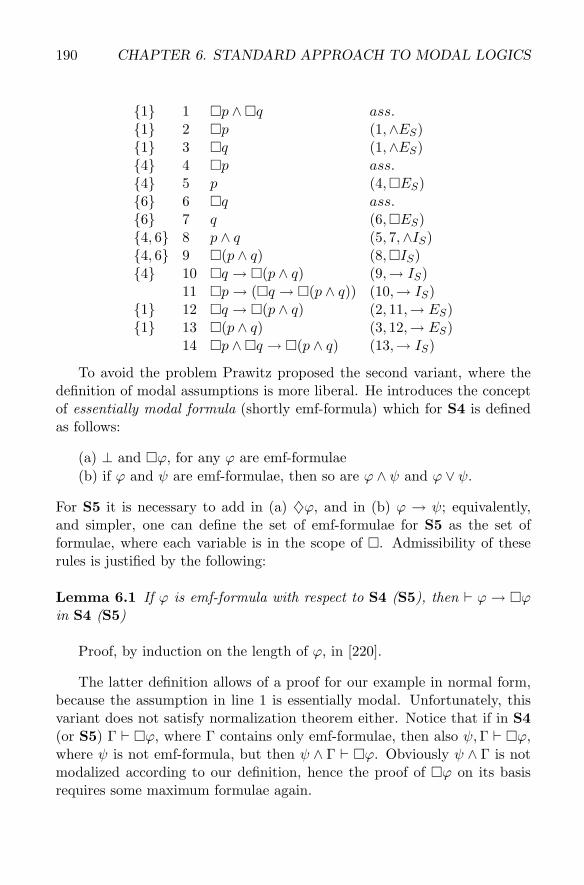
The above definition of modalized formulae provides a simple accountof rules but, unfortunately, forces us to construct unnecessarily long andcomplicated proofs – there is an example in Suppes’ format on the nextpage. The problem illustrated here is not only of practical nature, it hasalso some important theoretical aspect which we should describe briefly.Prawitz [220] has proved normalization theorem for many logics in ND-formalization. Unfortunately, not all proofs in his systems for S4 and S5may be transformed into normal form. For example, in displayed proofmaximum formulae are present in lines 10 (12) and 11.
4Corcoran in fact applied horizontal, instead of vertical, manner of displaying deriva-tions, but this is only a slight departure of no real importance.
190 CHAPTER 6. STANDARD APPROACH TO MODAL LOGICS
{1} 1 �p ∧ �q ass.{1} 2 �p (1,∧ES){1} 3 �q (1,∧ES){4} 4 �p ass.{4} 5 p (4,�ES){6} 6 �q ass.{6} 7 q (6,�ES){4, 6} 8 p ∧ q (5, 7,∧IS){4, 6} 9 �(p ∧ q) (8,�IS){4} 10 �q → �(p ∧ q) (9,→ IS)
11 �p→ (�q → �(p ∧ q)) (10,→ IS){1} 12 �q → �(p ∧ q) (2, 11,→ ES){1} 13 �(p ∧ q) (3, 12,→ ES)
14 �p ∧ �q → �(p ∧ q) (13,→ IS)
To avoid the problem Prawitz proposed the second variant, where thedefinition of modal assumptions is more liberal. He introduces the conceptof essentially modal formula (shortly emf-formula) which for S4 is definedas follows:
(a) ⊥ and �ϕ, for any ϕ are emf-formulae(b) if ϕ and ψ are emf-formulae, then so are ϕ ∧ ψ and ϕ ∨ ψ.
For S5 it is necessary to add in (a) ♦ϕ, and in (b) ϕ → ψ; equivalently,and simpler, one can define the set of emf-formulae for S5 as the set offormulae, where each variable is in the scope of �. Admissibility of theserules is justified by the following:
Lemma 6.1 If ϕ is emf-formula with respect to S4 (S5), then � ϕ → �ϕin S4 (S5)
Proof, by induction on the length of ϕ, in [220].
The latter definition allows of a proof for our example in normal form,because the assumption in line 1 is essentially modal. Unfortunately, thisvariant does not satisfy normalization theorem either. Notice that if in S4(or S5) Γ � �ϕ, where Γ contains only emf-formulae, then also ψ,Γ � �ϕ,where ψ is not emf-formula, but then ψ ∧ Γ � �ϕ. Obviously ψ ∧ Γ is notmodalized according to our definition, hence the proof of �ϕ on its basisrequires some maximum formulae again.
6.2. SOME STANDARD ND FOR MODAL BASIC LOGICS 191
Remark 6.1 Prawitz presented also the third version of ND-systems forS4 and S5 which was believed to satisfy normalization theorem, but it isa solution of rather different sort. It is admissible in them to apply �introduction to formula based on any assumption, on condition that thereare some modalized formulae in the proof connecting these assumptions anda formula in question. Prawitz has proved normalization theorem for thisversion in the language with no ∨,∃,♦; it was recently extended for S5to full language by Martins and Martins [184]. In fact, Prawitz solution israther a variant of Fitch’s approach described in Section 6.3. It is also of nopractical importance because it only shows what to check in a completedproof, not how to construct it. However, Sieg and Cittadini [255] providedextension of their intercalation calculus to S4 based on this solution.
Anyway, it was noticed by Medeiros [189] that original proof of Prawitzfor S4 is erroneous. She provided slightly modified system but her nor-malization proof is also incomplete, as was noticed by Andou [7]. On theother hand, von Plato [212] has shown that even the first version for S4 isnormalizable if we use in classical basis his general elimination rules; in caseof � (in F-format) it takes the form:
(�EG) if ϕ � ψ then Γ,�ϕ � ψ ♣
The serious drawback of this approach is due to its limited scope of ap-plication. It is not incidental that such systems were devised only for S4 andS5. These are the logics for which modal rules from SC-formalizations haveΓ� and Δ� defined as subsets of Γ and Δ; no modification of formulae fromΓ ∪ Δ is involved. We can obtain adequate formalizations also for regularcounterpart of S4 or for monotonic versions of these logics by demandingnonempty (or singular) set of modalized assumptions for premises in case of� introduction. But it is certainly not obvious how to extend this approachto other logics.
We do not claim however that some other extensions of Suppes’ formatND are not possible if we additionaly use some rules of different character.In Section 6.4.3 we propose alternative way of formalization suitable forSuppes’ system; one may also consider an application of generalized rulesfor � elimination described in Remark 6.5. In [241] Satre proposed NDsystem in Suppes’ format for all modal logics considered in [173] whichinvolves Curry’s rules but add also other rules for � introduction. AlthoughSatre underlines the influence of Ohnishi/Matsumoto for his work, his ruleshave a different character. The problem is basically with adaptation of SCrules to ND in Gentzen’s S-format. If we are ready to admit rules which
192 CHAPTER 6. STANDARD APPROACH TO MODAL LOGICS
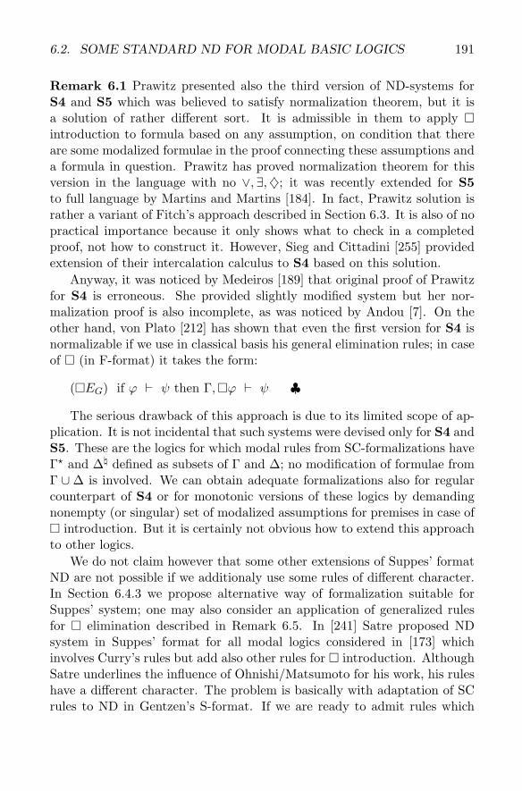
perform some operations also on the set of assumptions, then we are freeto take any of the SC rules presented in Section 6.1. This is the approachrepresented in appendix of [136]. But it leads to some problems with therealization of such calculus, if we prefer to use Suppes’ format, i.e. not touse all sequents but just formulae (=succedents) with records of numbers ofassumptions (=antecedent). In Satre’s approach no operations are allowedon assumptions at the cost of having more complex rules. For K a suitablerule has the following form:
(S-K) Γ1 ⇒ �ϕ1; ...; Γn ⇒ �ϕn; ϕ1, ..., ϕn ⇒ ψ / Γ1, ...,Γn ⇒ �ψ
By introduction of suitable restrictions on this rule and on (�I) andaddition of sequent forms of rules corresponding to D or T (like (�ES)stated above) Satre is able to obtain formalizations of all normal and regularlogics from [173] (for quasi-regular ones he must add some other rules aswell). We omit the details but present a proof of K as an example ofapplication of (S-K):
{1} 1 �(p→ q) ass.{2} 2 �p ass.{3} 3 p→ q ass.{4} 4 p ass.{3, 4} 5 q (3, 4,→ ES){1, 2} 6 �q (1, 2, 5, S-K){1} 7 �p→ �q (6,→ IS)
8 �(p→ q) → (�p→ �q) (7,→ IS)
6.2.2 Modalization of Rules
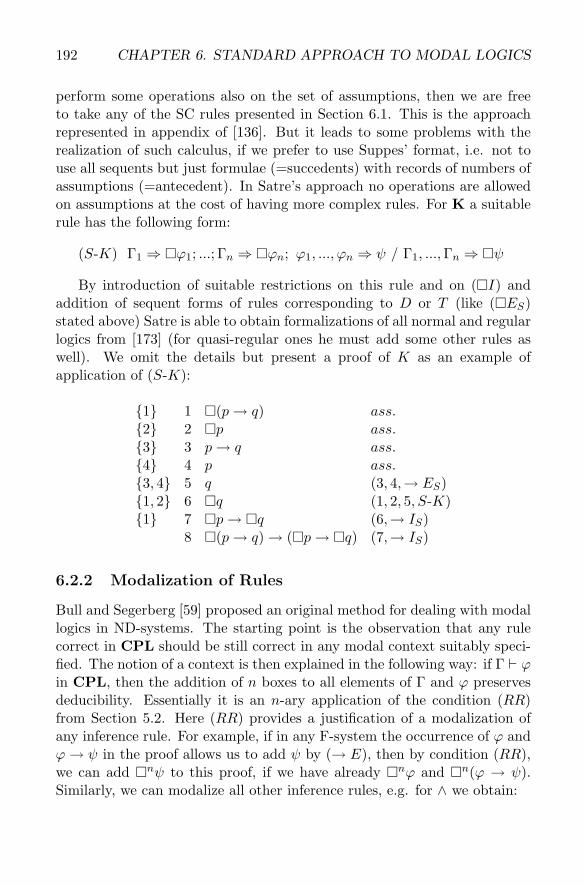
Bull and Segerberg [59] proposed an original method for dealing with modallogics in ND-systems. The starting point is the observation that any rulecorrect in CPL should be still correct in any modal context suitably speci-fied. The notion of a context is then explained in the following way: if Γ � ϕin CPL, then the addition of n boxes to all elements of Γ and ϕ preservesdeducibility. Essentially it is an n-ary application of the condition (RR)from Section 5.2. Here (RR) provides a justification of a modalization ofany inference rule. For example, if in any F-system the occurrence of ϕ andϕ→ ψ in the proof allows us to add ψ by (→ E), then by condition (RR),we can add �nψ to this proof, if we have already �nϕ and �n(ϕ → ψ).Similarly, we can modalize all other inference rules, e.g. for ∧ we obtain:
6.2. SOME STANDARD ND FOR MODAL BASIC LOGICS 193
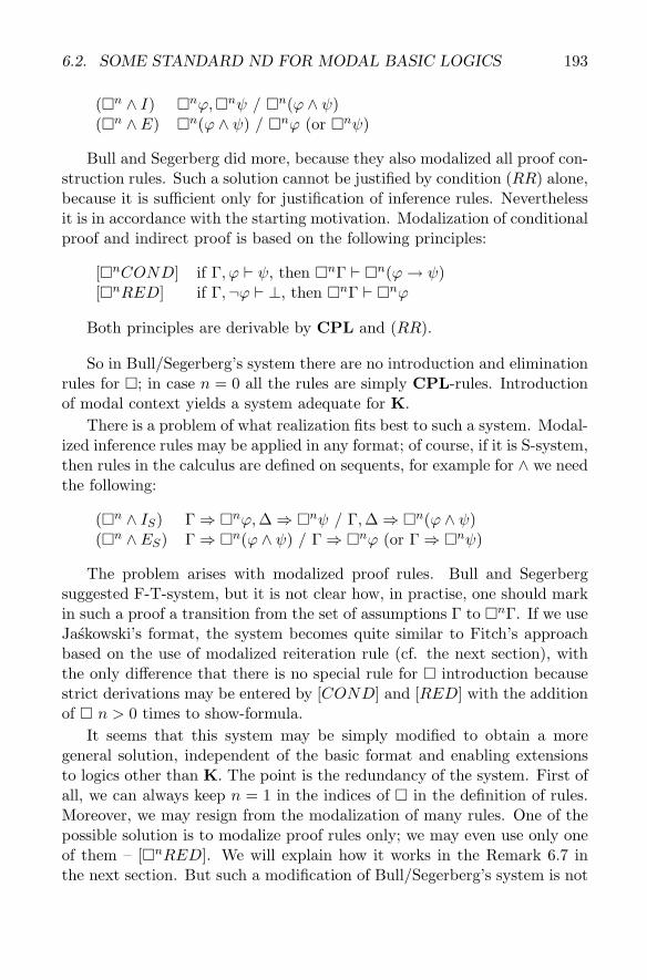
(�n ∧ I) �nϕ,�nψ / �n(ϕ ∧ ψ)(�n ∧ E) �n(ϕ ∧ ψ) / �nϕ (or �nψ)
Bull and Segerberg did more, because they also modalized all proof con-struction rules. Such a solution cannot be justified by condition (RR) alone,because it is sufficient only for justification of inference rules. Neverthelessit is in accordance with the starting motivation. Modalization of conditionalproof and indirect proof is based on the following principles:
[�nCOND] if Γ, ϕ � ψ, then �nΓ � �n(ϕ→ ψ)[�nRED] if Γ,¬ϕ � ⊥, then �nΓ � �nϕ
Both principles are derivable by CPL and (RR).
So in Bull/Segerberg’s system there are no introduction and eliminationrules for �; in case n = 0 all the rules are simply CPL-rules. Introductionof modal context yields a system adequate for K.
There is a problem of what realization fits best to such a system. Modal-ized inference rules may be applied in any format; of course, if it is S-system,then rules in the calculus are defined on sequents, for example for ∧ we needthe following:
(�n ∧ IS) Γ ⇒ �nϕ,Δ ⇒ �nψ / Γ,Δ ⇒ �n(ϕ ∧ ψ)(�n ∧ ES) Γ ⇒ �n(ϕ ∧ ψ) / Γ ⇒ �nϕ (or Γ ⇒ �nψ)
The problem arises with modalized proof rules. Bull and Segerbergsuggested F-T-system, but it is not clear how, in practise, one should markin such a proof a transition from the set of assumptions Γ to �nΓ. If we useJaskowski’s format, the system becomes quite similar to Fitch’s approachbased on the use of modalized reiteration rule (cf. the next section), withthe only difference that there is no special rule for � introduction becausestrict derivations may be entered by [COND] and [RED] with the additionof � n > 0 times to show-formula.
It seems that this system may be simply modified to obtain a moregeneral solution, independent of the basic format and enabling extensionsto logics other than K. The point is the redundancy of the system. First ofall, we can always keep n = 1 in the indices of � in the definition of rules.Moreover, we may resign from the modalization of many rules. One of thepossible solution is to modalize proof rules only; we may even use only oneof them – [�nRED]. We will explain how it works in the Remark 6.7 inthe next section. But such a modification of Bull/Segerberg’s system is not
194 CHAPTER 6. STANDARD APPROACH TO MODAL LOGICS
very original; it is in fact a variant of Fitch’s system.A better solution, still in accordance with the original motivation, is to
limit the modalization only to inference rules. It is based on the naturalinterpretation of condition (RR), and ND-system thus obtained is not avariant of Fitch’s system anymore, because it forces us to use different proofstrategies. To get an adequate formalization for K without any modificationof proof rules, one must allow of a modalization of inference rules withempty set of premises, which is simply an application of (RG). Althoughformalization of this kind is format-insensitive, practically it is simpler tocombine it with S-format because of the last proviso; in Jaskowski formatit is not immediately evident if a formula is really not dependent on anyassumptions.
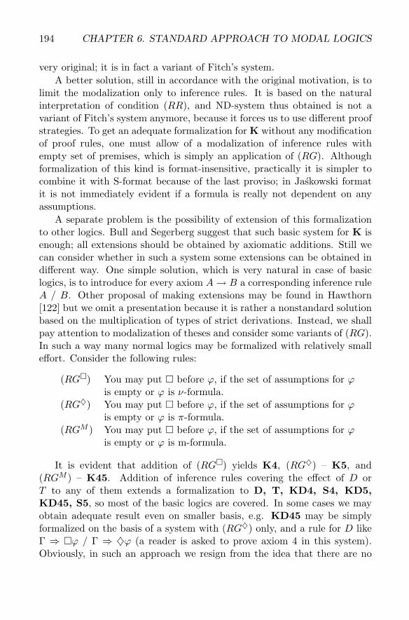
A separate problem is the possibility of extension of this formalizationto other logics. Bull and Segerberg suggest that such basic system for K isenough; all extensions should be obtained by axiomatic additions. Still wecan consider whether in such a system some extensions can be obtained indifferent way. One simple solution, which is very natural in case of basiclogics, is to introduce for every axiom A→ B a corresponding inference ruleA / B. Other proposal of making extensions may be found in Hawthorn[122] but we omit a presentation because it is rather a nonstandard solutionbased on the multiplication of types of strict derivations. Instead, we shallpay attention to modalization of theses and consider some variants of (RG).In such a way many normal logics may be formalized with relatively smalleffort. Consider the following rules:
(RG�) You may put � before ϕ, if the set of assumptions for ϕis empty or ϕ is ν-formula.
(RG♦) You may put � before ϕ, if the set of assumptions for ϕis empty or ϕ is π-formula.
(RGM ) You may put � before ϕ, if the set of assumptions for ϕis empty or ϕ is m-formula.
It is evident that addition of (RG�) yields K4, (RG♦) – K5, and(RGM ) – K45. Addition of inference rules covering the effect of D orT to any of them extends a formalization to D, T, KD4, S4, KD5,KD45, S5, so most of the basic logics are covered. In some cases we mayobtain adequate result even on smaller basis, e.g. KD45 may be simplyformalized on the basis of a system with (RG♦) only, and a rule for D likeΓ ⇒ �ϕ / Γ ⇒ ♦ϕ (a reader is asked to prove axiom 4 in this system).Obviously, in such an approach we resign from the idea that there are no
6.3. MODALIZATION OF REITERATION RULE 195
specific rules for modal functors but it seems that adding axioms to systemfor K is not better.
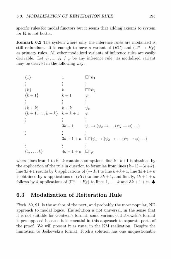
Remark 6.2 The system where only the inference rules are modalized isstill redundant. It is enough to have a variant of (RG) and (�n → ES)as primary rules. All other modalized variants of inference rules are easilyderivable. Let ψ1, ..., ψk / ϕ be any inference rule; its modalized variantmay be derived in the following way:
{1} 1 �nψ1...
......
{k} k �nψk{k + 1} k + 1 ψ1...
......
{k + k} k + k ψk{k + 1, . . . , k + k} k + k + 1 ϕ...
......
3k + 1 ψ1 → (ψ2 → . . . (ψk → ϕ) . . .)...
......
3k + 1 + n �n(ψ1 → (ψ2 → . . . (ψk → ϕ) . . .)...
......
{1, . . . , k} 4k + 1 + n �nϕ
where lines from 1 to k+k contain assumptions, line k+k+1 is obtained bythe application of the rule in question to formulae from lines (k+1)−(k+k),line 3k+1 results by k applications of (→ IS) to line k+k+1, line 3k+1+nis obtained by n applications of (RG) to line 3k+ 1, and finally, 4k+ 1 + nfollows by k applications of (�n → ES) to lines 1, . . . , k and 3k + 1 + n. ♣
6.3 Modalization of Reiteration Rule
Fitch [89, 91] is the author of the next, and probably the most popular, NDapproach to modal logics. His solution is not universal, in the sense thatit is not suitable for Gentzen’s format; some variant of Jaskowski’s formatis presupposed because it is essential in this approach to separate parts ofthe proof. We will present it as usual in the KM realization. Despite thelimitation to Jaskowski’s format, Fitch’s solution has one unquestionable
196 CHAPTER 6. STANDARD APPROACH TO MODAL LOGICS
advantage – the scope: [89] contains only ND system for T and S4,5 [91]provides counterparts for some deontic logics. Siemens [256] extends thisformalization further, finally in Fitting [93] one can find a uniform formaliza-tion for many regular and normal logics. Fitch’s approach was generalizedeven further: for basic normal logics of strict implication by Cerrato [66],for many relevance logics by Anderson and Belnap [5] and for conditionallogics by Thomason [275]. Some extensions, due to Indrzejczak, to bimodaltemporal logics [140] and to first-order modal logics [141] will be presentedbelow. These are only some examples of application of Fitch’s idea.
We will show that this approach is the closest relative of standard SCand TS for modal logics. In case of basic logics we may even say that theseapproaches are equivalent in the sense that every logic adequately formalizedin SC (or TS) is formalizable in Fitch-style ND and vice versa. This strictcorrespondence is destroyed for some of these modal logics which use modalSC (or TS) rules with more premises than one.
The basic idea of Fitch’s approach is the introduction of special categoryof subproofs called strict or modal. In ND-system for CPL one can use anyU-formula from an open derivation of k-degree in open derivation of anyhigher degree which is nested in it. In case of modal logic, if new subderiva-tion is strict, then only special sort of U-formulae from outer derivation(or formulae obtained by some operation performed on them) may be used.The logic in question decides what kind of U-formulae (or their derivatives)is admissible. The idea is that one can obtain ND formalizations for dif-ferent logics only by modeling the set of suitable formulae, keeping all theinference and proof rules intact.
Technically, the problem of control over admissible formulae on the levelof realization is solved by the introduction of reiteration rule (Reit) whichregulates the transfer of formulae from a parent derivation to its subderiva-tions. We did not introduce explicitly this rule to KM-CPL since transferof formulae was not restricted and the definition of proof was simpler oncondition that we can use any U-formula in current subderivation. In modalsetting such a rule must be explicitly stated and every application of anyinference rule must be performed only on premises which are present in thecurrent subderivation.
If we restrict our consideration to L�, then to obtain an adequate for-malization of K we must add to the calculus for CPL only one rule of proofconstruction:
5In fact, Fitch did not realize that he formalized T; he claimed that his rules gives“almost S2”.
6.3. MODALIZATION OF REITERATION RULE 197
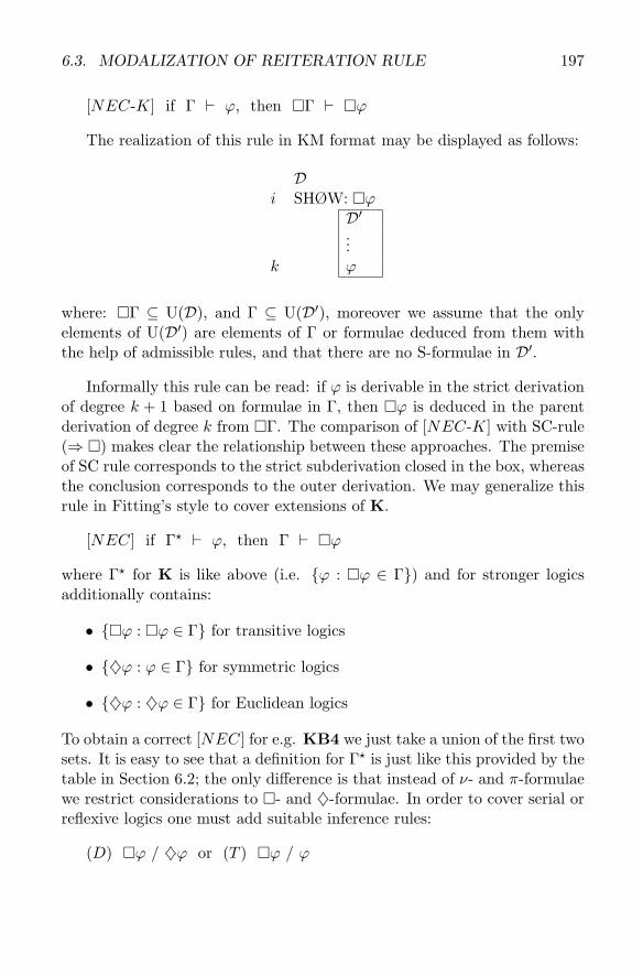
[NEC-K] if Γ � ϕ, then �Γ � �ϕ
The realization of this rule in KM format may be displayed as follows:
Di SHØW: �ϕ
D′...
k ϕ
where: �Γ ⊆ U(D), and Γ ⊆ U(D′), moreover we assume that the onlyelements of U(D′) are elements of Γ or formulae deduced from them withthe help of admissible rules, and that there are no S-formulae in D′.
Informally this rule can be read: if ϕ is derivable in the strict derivationof degree k + 1 based on formulae in Γ, then �ϕ is deduced in the parentderivation of degree k from �Γ. The comparison of [NEC-K] with SC-rule(⇒ �) makes clear the relationship between these approaches. The premiseof SC rule corresponds to the strict subderivation closed in the box, whereasthe conclusion corresponds to the outer derivation. We may generalize thisrule in Fitting’s style to cover extensions of K.
[NEC] if Γ� � ϕ, then Γ � �ϕ
where Γ� for K is like above (i.e. {ϕ : �ϕ ∈ Γ}) and for stronger logicsadditionally contains:
• {�ϕ : �ϕ ∈ Γ} for transitive logics
• {♦ϕ : ϕ ∈ Γ} for symmetric logics
• {♦ϕ : ♦ϕ ∈ Γ} for Euclidean logics
To obtain a correct [NEC] for e.g. KB4 we just take a union of the first twosets. It is easy to see that a definition for Γ� is just like this provided by thetable in Section 6.2; the only difference is that instead of ν- and π-formulaewe restrict considerations to �- and ♦-formulae. In order to cover serial orreflexive logics one must add suitable inference rules:
(D) �ϕ / ♦ϕ or (T ) �ϕ / ϕ
198 CHAPTER 6. STANDARD APPROACH TO MODAL LOGICS
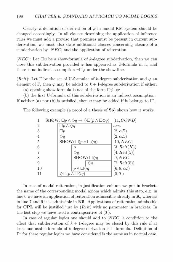
Clearly, a definition of derivation of ϕ in modal KM system should bechanged accordingly. In all clauses describing the application of inferencerules we must add a proviso that premises must be present in current sub-derivation, we must also state additional clauses concerning closure of asubderivation by [NEC] and the application of reiteration.
[NEC]: Let �ϕ be a show-formula of k-degree subderivation, then we canclose this subderivation provided ϕ has appeared as U-formula in it, andthere is no indirect assumption ¬�ϕ under the show-line.
(Reit): Let Γ be the set of U-formulae of k-degree subderivation and ϕ anelement of Γ, then ϕ may be added to k + 1-degree subderivation if either:
(a) opening show-formula is not of the form �ψ, or(b) the first U-formula of this subderivation is an indirect assumption.
If neither (a) nor (b) is satisfied, then ϕ may be added if it belongs to Γ�.
The following example (a proof of a thesis of S5) shows how it works.
1 SHØW: �p ∧ ♦q → ♦�(p ∧ �♦q) [11, COND]2 �p ∧ ♦q ass.3 �p (2, αE)4 ♦q (2, αE)5 SHØW: �(p ∧ �♦q) [10, NEC]6 p (3, Reit(K))7 ♦q (4, Reit(5))8 SHØW: �♦q [9, NEC]9 ♦q (7, Reit(5))10 p ∧ �♦q (6, 8, αI)11 ♦�(p ∧ �♦q) (5, T )
In case of modal reiteration, in justification column we put in bracketsthe name of the corresponding modal axiom which admits this step, e.g. inline 6 we have an application of reiteration admissible already in K, whereasin line 7 and 9 it is admissible in K5. Applications of reiteration admissiblefor CPL will be justified just by (Reit) with no parameter in brackets. Inthe last step we have used a contrapositive of (T ).
In case of regular logics one should add to [NEC] a condition to theeffect that subderivation of k + 1-degree may be closed by this rule if atleast one usable-formula of k-degree derivation is �-formula. Definition of� for these regular logics we have considered is the same as in normal case.
6.3. MODALIZATION OF REITERATION RULE 199
It is quite easy to prove that this system is adequate with respect to allbasic normal and regular logics. Completeness requires proofs of suitableaxioms, which is routine; (RG) and (RR) is simulated by [NEC]. Soundnessis also not very difficult to prove; we will do it in the next section.
Remark 6.3 Fitting [93] in his formalization for regular logics used differentbut equivalent solution; instead of [NEC] he proposed a proof constructionrule based on the principle:
[MOD] if Γ� � ϕ ∨ ψ, then Γ � ♦ϕ ∨ �ψ ♣
Remark 6.4 Rules [NEC] and (Reit) may be significantly simplified in ourversion of KM. First, as we remarked in Chapter 2, one can eliminate fromKM both [RED] and the rule for entering indirect assumptions, becausethese rules are not necessary in the system with our set of inference rules.In so modified system both [NEC] and (Reit) may be formulated as follows:
[NEC ′] Let �ϕ be a show-formula of k-degree subderivation, where ϕ hasappeared as a usable-formula, then we can close this subderivation, providedall its usable-formulae justified by (Reit′) belong to Γ�.
(Reit′) Let Γ be the set of usable-formulae of k-degree subderivation, thenwe may add to k + 1-degree subderivation either:
(a) ϕ ∈ Γ�, if show-formula of this subderivation is �-formula, or
(b) ϕ ∈ Γ
Even if [RED] and indirect assumptions are kept intact, both rules can besimplified in case of reflexive logics; we can use [NEC ′] and the following:
(Reit′′) Let Γ be the set of usable-formulae of k-degree subderivation, thenwe may add to k + 1-degree subderivation ϕ belonging either to Γ� or to Γ
This simplification is due to the fact that although in case of [NEC],(Reit) must be restricted to Γ�, then in case of other rules of closing aderivation both elements of Γ and Γ� are admissible in reflexive logics, be-cause formulae from Γ� may be inferred by the application of (T ). Alsothe condition that indirect assumption should not be present in the deriva-tion to be closed by [NEC] is not needed because for T, and its extensionstreated here, one can prove the following as an admissible rule:
200 CHAPTER 6. STANDARD APPROACH TO MODAL LOGICS
[NECT ] if Γ�,¬�ϕ � ϕ, then Γ � �ϕ
Our primary formulation, despite the complications in the definitionof (Reit), has one serious advantage. All the necessary restrictions arestated as the conditions to be satisfied before we apply the rule, hencewe do not need to check a finished proof whether there are some mistakes.Simpler formulations, often found in literature, usually require some controlof correctness after the proof is completed. ♣
Remark 6.5 The drawback of this formalization is the lack of any rule of� elimination for logics weaker then T; in case of D one can use in thisrole an inference rule (D) �ϕ / ♦ϕ, but it is an ad hoc solution. Someauthors, like Garson [105], prefer yet another terminological convention.Given the definition of Γ� for K, it is possible to define (Reit(K)) for strictderivation as a kind of (�E), while allowing simple transfer of formulae inordinary subderivations. This solution has also some disadvantages, whenwe consider how to obtain extensions of K. These forms of reiteration hardlymay be treated in a similar way, because e.g. in K4, � is not only eliminatedbut also the whole �-formula is put in a strict subderivation. Garson simplyapplies Bull and Segerberg’s solution and add suitable axioms.
A different solution is possible, at least for some logics which are not re-flexive, if we consider some variants of (�E) defined on modalized formulae,e.g.:
(�E�) �ϕ / ϕ, for any �-formula ϕ(�E♦) �ϕ / ϕ, for any ♦-formula ϕ(�E�♦) �ϕ / ϕ, for any m-formula ϕ
(�E�) may be added to K5 and its extensions, (�E♦) to KD4, whichimplies that (�E�♦) is a suitable rule for KD45. In this way, at least somelogics without T have (�E) of some sort, but it should be noticed that allthese rules are in fact derivable in the basic formalization, what is more,they cannot replace the rule (D) in KD4, or KD5. The exception is KD45,a very important epistemic logic; instead of replacement of (�E) by (D) inND-S5, one can use (�E♦), which is simpler and more natural. Proofs ofK, 4, 5 run like in ND-S5, it is enough to show that D is also provable; as ashortcut we will use a secondary rule (R5) ♦�ϕ / �ϕ, which is obviouslyderivable either.
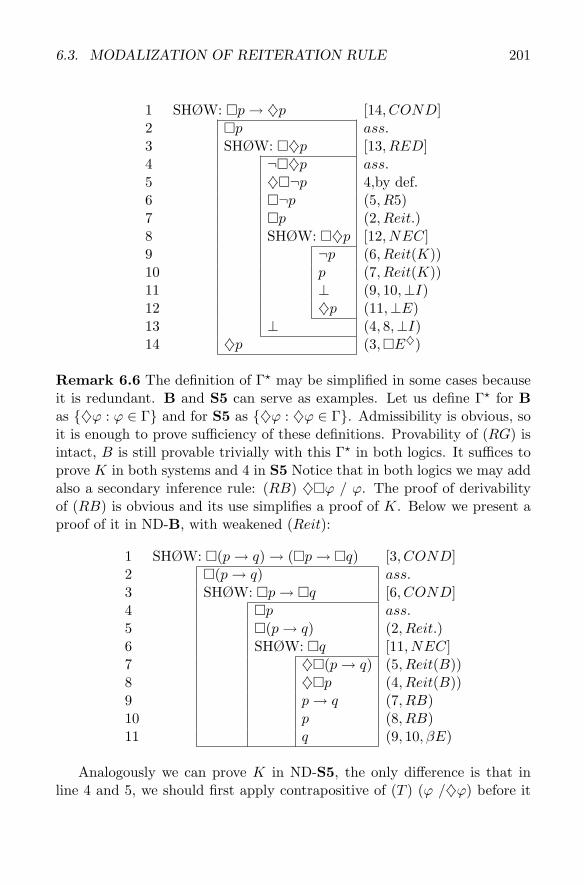
6.3. MODALIZATION OF REITERATION RULE 201
1 SHØW: �p→ ♦p [14, COND]2 �p ass.3 SHØW: �♦p [13, RED]4 ¬�♦p ass.5 ♦�¬p 4,by def.6 �¬p (5, R5)7 �p (2, Reit.)8 SHØW: �♦p [12, NEC]9 ¬p (6, Reit(K))10 p (7, Reit(K))11 ⊥ (9, 10,⊥I)12 ♦p (11,⊥E)13 ⊥ (4, 8,⊥I)14 ♦p (3,�E♦)
Remark 6.6 The definition of Γ� may be simplified in some cases becauseit is redundant. B and S5 can serve as examples. Let us define Γ� for Bas {♦ϕ : ϕ ∈ Γ} and for S5 as {♦ϕ : ♦ϕ ∈ Γ}. Admissibility is obvious, soit is enough to prove sufficiency of these definitions. Provability of (RG) isintact, B is still provable trivially with this Γ� in both logics. It suffices toprove K in both systems and 4 in S5 Notice that in both logics we may addalso a secondary inference rule: (RB) ♦�ϕ / ϕ. The proof of derivabilityof (RB) is obvious and its use simplifies a proof of K. Below we present aproof of it in ND-B, with weakened (Reit):
1 SHØW: �(p→ q) → (�p→ �q) [3, COND]2 �(p→ q) ass.3 SHØW: �p→ �q [6, COND]4 �p ass.5 �(p→ q) (2, Reit.)6 SHØW: �q [11, NEC]7 ♦�(p→ q) (5, Reit(B))8 ♦�p (4, Reit(B))9 p→ q (7, RB)10 p (8, RB)11 q (9, 10, βE)
Analogously we can prove K in ND-S5, the only difference is that inline 4 and 5, we should first apply contrapositive of (T ) (ϕ /♦ϕ) before it
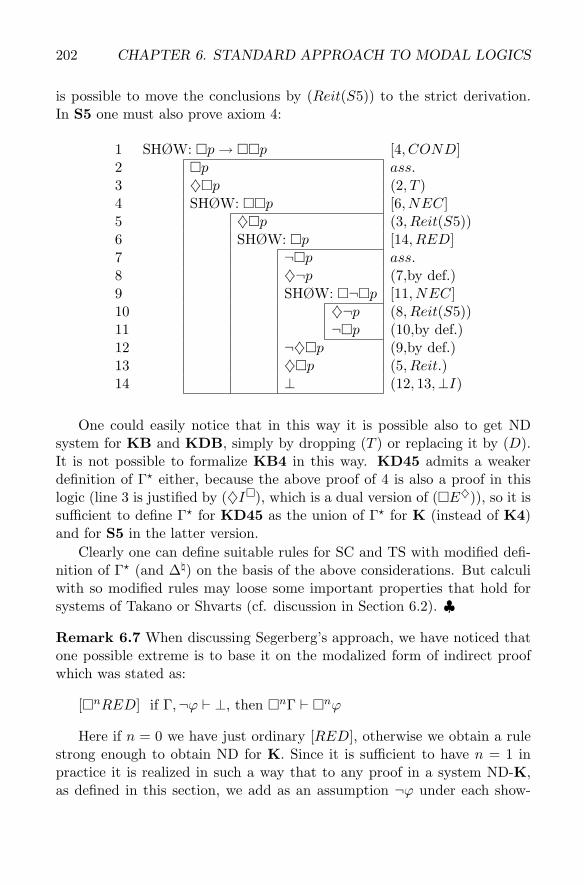
202 CHAPTER 6. STANDARD APPROACH TO MODAL LOGICS
is possible to move the conclusions by (Reit(S5)) to the strict derivation.In S5 one must also prove axiom 4:
1 SHØW: �p→ ��p [4, COND]2 �p ass.3 ♦�p (2, T )4 SHØW: ��p [6, NEC]5 ♦�p (3, Reit(S5))6 SHØW: �p [14, RED]7 ¬�p ass.8 ♦¬p (7,by def.)9 SHØW: �¬�p [11, NEC]10 ♦¬p (8, Reit(S5))11 ¬�p (10,by def.)12 ¬♦�p (9,by def.)13 ♦�p (5, Reit.)14 ⊥ (12, 13,⊥I)
One could easily notice that in this way it is possible also to get NDsystem for KB and KDB, simply by dropping (T ) or replacing it by (D).It is not possible to formalize KB4 in this way. KD45 admits a weakerdefinition of Γ� either, because the above proof of 4 is also a proof in thislogic (line 3 is justified by (♦I�), which is a dual version of (�E♦)), so it issufficient to define Γ� for KD45 as the union of Γ� for K (instead of K4)and for S5 in the latter version.
Clearly one can define suitable rules for SC and TS with modified defi-nition of Γ� (and Δ�) on the basis of the above considerations. But calculiwith so modified rules may loose some important properties that hold forsystems of Takano or Shvarts (cf. discussion in Section 6.2). ♣
Remark 6.7 When discussing Segerberg’s approach, we have noticed thatone possible extreme is to base it on the modalized form of indirect proofwhich was stated as:
[�nRED] if Γ,¬ϕ � ⊥, then �nΓ � �nϕ
Here if n = 0 we have just ordinary [RED], otherwise we obtain a rulestrong enough to obtain ND for K. Since it is sufficient to have n = 1 inpractice it is realized in such a way that to any proof in a system ND-K,as defined in this section, we add as an assumption ¬ϕ under each show-
6.4. RULES FOR POSSIBILITY 203
formula �ϕ, and change a justification from [NEC], to [�nRED]. Clearly,for stronger logics we must keep suitable modal reiteration rule as definedabove, but it still works because the following rule is obviously admissible:
if Γ�,¬ϕ � ⊥, then Γ � �ϕ
In practise it is easy to realise – just add an indirect assumption to everystrict subderivation. ♣
6.4 Rules for Possibility
So far we have used ♦ as a definitional shortcut, which was in accordancewith the usual practice of many authors. However, the problem of formal-ization of ♦ is sufficiently interesting in itself to be described separately.Moreover, as we shall see, an application of ♦ as primitive opens the way todefine modal ND which is not committed to Jaskowski’s format, but maybe used with any other format presented in Chapter 2.
6.4.1 Original Fitch’s System
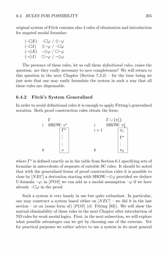
In the original system of Fitch for T and S4, ♦ was in fact treated as anindependent functor and characterized by the pair of rules of introductionand elimination. On the level of calculus of our ND system the first of themis an introduction rule:
(♦I) ϕ / ♦ϕ
which is of course normal only for reflexive logics. The second one is anotherproof construction rule:
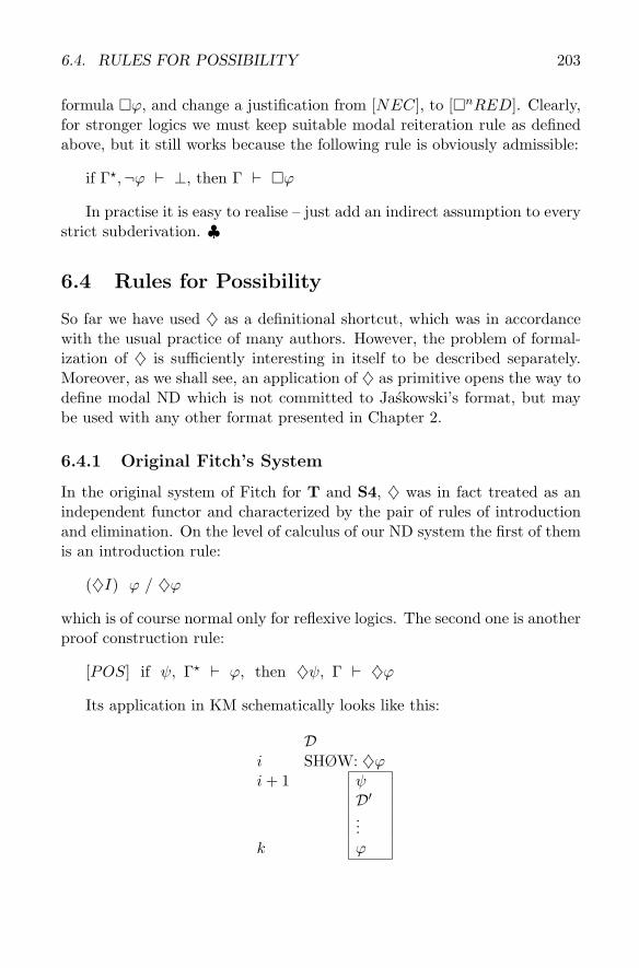
[POS] if ψ, Γ� � ϕ, then ♦ψ, Γ � ♦ϕ
Its application in KM schematically looks like this:
Di SHØW: ♦ϕi+ 1 ψ
D′...
k ϕ
204 CHAPTER 6. STANDARD APPROACH TO MODAL LOGICS
where: �Γ ∪ {♦ψ} ⊆ U(D), Γ ⊆ U(D′), and ψ is a modal assumption.Moreover, we assume that the only elements of U(D′) are elements of Γ orformulae deduced from Γ ∪ {ψ} with the help of admissible rules, and thatthere are no S-formulae in D′.
On the level of realization we must add to KM two rules that corre-spond to [POS]; one for closing a derivation and one for entering modalassumption:
[POS] Let ♦ϕ be the show-formula of k-degree subderivation with the firstU-formula being modal assumption, then we can close this subderivation,provided ϕ has appeared in it as U-formula.
(mod.ass.) If ♦ψ is U-formula of k-degree subderivation and ♦ϕ is S-formulaentering k+1-degree subderivation, then we may add ψ as a modal assump-tion of the k + 1-degree derivation
In fact, also (Reit) should be modified; we introduce the version whichworks for the system in which both [NEC] and [POS] are counted as prim-itive. Because of the stylistic reasons it will be defined dually to our officialformulation of (Reit) from Section 6.3.
Let Γ be the set of U-formulae of k-degree subderivation and ϕ ∈ Γ�,we may put ϕ into subderivation of k+ 1-degree by (Reit) if at least one ofthe following conditions is satisfied:
(a) show-formula of this subderivation is �ψ and the first U-formula ofthis subderivation is not an indirect assumption
(b) the first U-formula of this subderivation is modal assumption;if neither (a) nor (b) is satisfied, then we may put into this derivation anyϕ ∈ Γ
One should notice that although an introduction of modal assumption isan optional element (we may have some ♦-formula as show-formula but totry to close this subderivation by different rule), its presence is a necessarycondition to close the derivation by [POS].
Introduction of special rules for ♦ is very convenient in practice. Veryoften we may produce shorter proofs for many theorems (and usually withrelatively smaller effort). But one should notice that the system containingboth [NEC] and [POS] in such a version is still incomplete in the languagewith both modalities taken as primitive. To overcome the problem the
6.4. RULES FOR POSSIBILITY 205
original system of Fitch contains also 4 rules of elimination and introductionfor negated modal formulae:
(¬�E) ¬�ϕ / ♦¬ϕ(¬�I) ♦¬ϕ / ¬�ϕ(¬♦E) ¬♦ϕ / �¬ϕ(¬♦I) �¬ϕ / ¬♦ϕ
The presence of these rules, let us call them definitional rules, raises thequestion: are they really necessary to save completeness? We will return tothis question in the next Chapter (Section 7.3.2) – for the time being wejust note that one may easily formulate the system in such a way that allthese rules are dispensable.
6.4.2 Fitch’s System Generalized
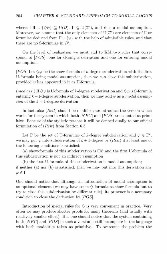
In order to avoid definitional rules it is enough to apply Fitting’s generalizednotation. Both proof construction rules obtain the form:
Γ Γ ∪ {πi1}i SHØW: νi i SHØW: πi2
Γ� i+ 1 π1... Γ�...
...k ν k π2
where Γ� is defined exactly as in the table from Section 6.1 specifying sets offormulae in antecedents of sequents of suitable SC rules. It should be notedthat with the generalized forms of proof construction rules it is possible toclose by [NEC] a derivation starting with SHOW:¬♦ϕ provided we deduceU-formula ¬ϕ; in [POS] we can add as a modal assumption ¬ϕ if we havealready ¬�ϕ in the proof.
Such a system is very handy in use but quite redundant. In particular,one may construct a system based either on [NEC] – we did it in the lastsection – or on (some form of) [POS] (cf. Fitting [93]). We will show themutual eliminability of these rules in the next Chapter after introduction ofND rules for weak modal logics. First, in the next subsection, we will explorewhat possible advantages can we get by choosing one of the extreme. Yetfor practical purposes we rather advice to use a system in its most general
206 CHAPTER 6. STANDARD APPROACH TO MODAL LOGICS
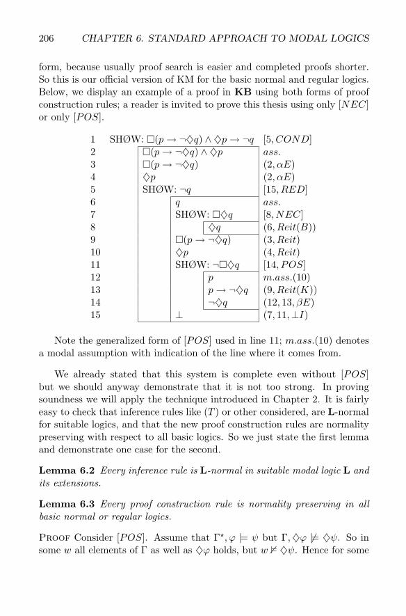
form, because usually proof search is easier and completed proofs shorter.So this is our official version of KM for the basic normal and regular logics.Below, we display an example of a proof in KB using both forms of proofconstruction rules; a reader is invited to prove this thesis using only [NEC]or only [POS].
1 SHØW: �(p→ ¬♦q) ∧ ♦p→ ¬q [5, COND]2 �(p→ ¬♦q) ∧ ♦p ass.3 �(p→ ¬♦q) (2, αE)4 ♦p (2, αE)5 SHØW: ¬q [15, RED]6 q ass.7 SHØW: �♦q [8, NEC]8 ♦q (6, Reit(B))9 �(p→ ¬♦q) (3, Reit)10 ♦p (4, Reit)11 SHØW: ¬�♦q [14, POS]12 p m.ass.(10)13 p→ ¬♦q (9, Reit(K))14 ¬♦q (12, 13, βE)15 ⊥ (7, 11,⊥I)
Note the generalized form of [POS] used in line 11; m.ass.(10) denotesa modal assumption with indication of the line where it comes from.
We already stated that this system is complete even without [POS]but we should anyway demonstrate that it is not too strong. In provingsoundness we will apply the technique introduced in Chapter 2. It is fairlyeasy to check that inference rules like (T ) or other considered, are L-normalfor suitable logics, and that the new proof construction rules are normalitypreserving with respect to all basic logics. So we just state the first lemmaand demonstrate one case for the second.
Lemma 6.2 Every inference rule is L-normal in suitable modal logic L andits extensions.
Lemma 6.3 Every proof construction rule is normality preserving in allbasic normal or regular logics.
Proof Consider [POS]. Assume that Γ�, ϕ |= ψ but Γ,♦ϕ �|= ♦ψ. So insome w all elements of Γ as well as ♦ϕ holds, but w � ♦ψ. Hence for some
6.4. RULES FOR POSSIBILITY 207
accessible w′, w′ � ϕ but w′� ψ. Consider elements of Γ�, all are taken by
modal reiteration from Γ, so there is a division of cases according to whichlogic is under consideration. Take K45 as an example and some arbitraryχ ∈ Γ�. Either �χ is in Γ or χ is in Γ and χ is some m-formula. In allcases w′ � χ. The first case holds for every model since w � �χ and Rww′.If χ is ν-formula it holds by transitivity of R; if χ is π-formula it holds byeuclideaness of R. So w′ � Γ� which implies that w′ � ψ and we have acontradiction. Thus Γ,♦ϕ |= ♦ψ.
Now, in order to prove soundness, we must change a bit a definitionof justified subproof. In fact, the introduction of reiteration rule leads tosimplification of this definition (and a proof) since we do not use as premisesof inference rules any formula from outer derivation. Let D be any proofand consider any subproof D′ of degree n > 0 contained in it. We say thatthis subproof is justified iff, Γ |= ψn, where ψn is the last formula of D′, andΓ is the set of all formulae of D′ introduced as assumption or by reiteration.
The proof proceeds as in Chapter 2, by double induction: on the depthk of D and on the length of its subproofs. In the basis we again consider allsubproofs of degree k, i.e. with no subproofs inside, and of length n, andshow that Γ |= ψi (1 ≤ i ≤ n) which implies that they are justified.
Basis: i = 1, so ψ1 is an assumption or a formula introduced by reiter-ation, and the claim follows by reflexivity and monotonicity of |=. Assumefor any i such that i < k ≤ n the claim holds and consider ψk. If ψk is byreiteration, then again Γ |= ψk by reflexivity and monotonicity. Otherwiseψk is deduced by some inference rule. By induction hypothesis our claimholds for all premises and by Lemma 6.2. the rule we have used is L-normal.Hence by transitivity of |= again Γ |= ψk which holds for n = k as well andwe are done.
In showing that every subproof of degree i is justified we proceed exactlyas in the proof of theorem 2.1. Every line of this subproof which is not acanceled S-line is justified by the same reasoning as in the basis, whereasprevious S-formulae need additional use of the induction hypothesis that allsubproofs of degree i+ 1 are justified. Let ψi be the first such a formula; wemust show that Γ |= ψi, where Γ is the set of all formulae in this subproofintroduced as an assumption or by reiteration. By the induction hypothesiswe have Γ′ |= χn, where χn is the last line of suitable subproof of degreei+1 and all elements of Γ′ are introduced as an assumption or by reiteration
208 CHAPTER 6. STANDARD APPROACH TO MODAL LOGICS
on the basis of some formulae occurring at this stage in the subproof ofdegree i. By Lemma 6.3. Γ′′ |= ψi because completion of this subproofwas obtained by some proof construction rule, and all rules are normalitypreserving. Now, Γ′′ is not necessarily a subset of Γ; it may contain formulaededuced from some elements of Γ by inference rules. Let Γ′′ = Δ ∪ Σ,where Δ ⊆ Γ and Σ is the set of k formulae introduced by some inferencerules. Consider the first χ ∈ Σ, by Lemma 6.2. and monotonicity Δ |= χsince the applied rule is normal. It holds also for the rest elements of Σby this lemma, monotonicity and possibly by transitivity of |=. So by kapplications of transitivity with respect to Γ′′ |= ψi and Δ |= χi, i ≤ kwe obtain Δ |= ψi and by monotonicity we finally conclude that Γ |= ψi.By the same argument we consecutively demonstrate that other previousS-lines in considered subproof of degree i are also justified. Since it holdsfor all subproofs, we obtain:
Theorem 6.1 (Soundness of KM for L) If Γ �L ϕ, then Γ |=L ϕ,where L is every basic regular or normal logic
Theorem 6.2 (Adequacy of KM for L) Every basic regular and nor-mal logic L is adequately characterized by KM-L.
Remark 6.8 It must be said that ordinary method of proving soundness ofND systems6 run into troubles in Fitch’s format ND for modal logics. It isnot clear how to transform into such a sequent a formula which is introducedby modal reiteration into a strict subderivation. Certainly if ϕ′ is such areiterated formula and ϕ its origin then it is rather not the case that Γ |= ϕimplies Γ |= ϕ′ (e.g. in K where ϕ is some νi and ϕ′ is ν). Similar problemsapply to justification of rules closing strict subproofs. Interesting innovationof this strategy of soundness proof may be found in [104, 105]. Garsoninstead of sets of active assumptions uses sequences of them (which, by theway, better complies with ordered character of subderivations in Jaskowski’sformat – cf. Section 2.4.3) and for every strict subproof introduces � asthe corresponding assumption. So for each formula in the proof we define asequent with this formula in the succedent and the sequence of formulae andboxes in the antecedent. This trick enables to keep the proof by inductionon the length of the whole derivation at the cost of small modification of aninterpretation of each line. Each sequence of active assumptions (formulae
6We mean soundness profs which are based on the transformation of every formula intoa sequent containing this formula in the succedent and the record of active assumptionsin the antecedent – cf. introductory remarks in Section 2.6.
6.4. RULES FOR POSSIBILITY 209
and boxes) is encoding a R-path in a partial description of a model, wherea formula from the succedent holds in the last world of this path. So wedo not prove, as in classical case, that Γ |= ϕ holds in line i provided someother statements of this sort hold in earlier lines. We rather prove thatM, w � ϕ, provided some other statements of this sort hold in earlier lines.♣
6.4.3 Modal Assumptions
In the previous subsection we have noticed that adequate formalization ofmodal logics can be based on only ♦ as a primitive functor. This possibilityis fully realized by Fitting [93], who presented two different ND systemsfor modal logics. One, called A-system, is based on [NEC], and the other,I-system, is based on some (stronger) form of [POS] which we name [⊥]F .
[⊥]F if Γ�, ψ � ⊥, then Γ,♦ψ � ⊥
The reason for preferring such a rule is connected with the fact that,in the context of normal logics, [POS] is too weak for complete charac-terization, although it is sufficient in weaker logics; we will show this inChapter 7.
This distinction is quite important for Fitting. He remarked that, withregard to proof construction, A-system is more connected with axiomaticformalizations based on (RG), whereas I-system is rather close to tableausystems. It makes I-system a better candidate as a potential proof-searchtool, whereas A-system is easier to use for completeness proof of nonana-lytic version. Semantic reasons for the distinction are even more important;strict derivations closed by [NEC] are interpreted in a different way thanthose closed by [⊥]F . In the former case strict derivation is a counterpartof an arbitrary chosen world (hence the name A-system per analogiam totraditional general-categorical A-statements). In the latter, it is a counter-part of some specific world in a Kripke model (hence the name I-systemas particular-categorical I-statement). This informal interpretation is forFitting a basis for the construction of respective soundness proofs for bothsystems.
So far we have run a different course, of mixing both systems, but fullcharacterization apart, we can ask a question: what advantages our pos-sibilistic approach, “possibly” offers? Previous presentation presupposedJaskowski’s format with the apparatus of strict derivations and restrictedreiterations. But the presence of modal assumptions can make at least
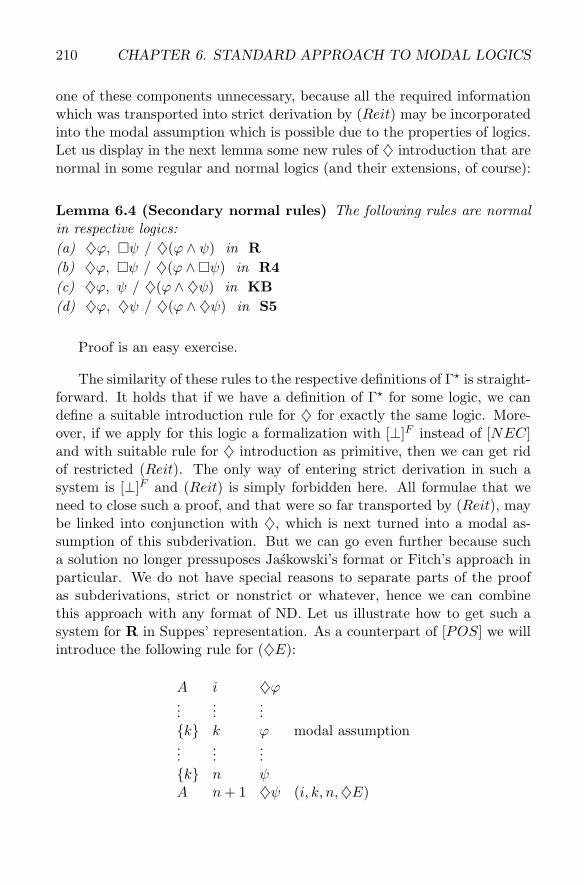
210 CHAPTER 6. STANDARD APPROACH TO MODAL LOGICS
one of these components unnecessary, because all the required informationwhich was transported into strict derivation by (Reit) may be incorporatedinto the modal assumption which is possible due to the properties of logics.Let us display in the next lemma some new rules of ♦ introduction that arenormal in some regular and normal logics (and their extensions, of course):
Lemma 6.4 (Secondary normal rules) The following rules are normalin respective logics:(a) ♦ϕ, �ψ / ♦(ϕ ∧ ψ) in R(b) ♦ϕ, �ψ / ♦(ϕ ∧ �ψ) in R4(c) ♦ϕ, ψ / ♦(ϕ ∧ ♦ψ) in KB(d) ♦ϕ, ♦ψ / ♦(ϕ ∧ ♦ψ) in S5
Proof is an easy exercise.
The similarity of these rules to the respective definitions of Γ� is straight-forward. It holds that if we have a definition of Γ� for some logic, we candefine a suitable introduction rule for ♦ for exactly the same logic. More-over, if we apply for this logic a formalization with [⊥]F instead of [NEC]and with suitable rule for ♦ introduction as primitive, then we can get ridof restricted (Reit). The only way of entering strict derivation in such asystem is [⊥]F and (Reit) is simply forbidden here. All formulae that weneed to close such a proof, and that were so far transported by (Reit), maybe linked into conjunction with ♦, which is next turned into a modal as-sumption of this subderivation. But we can go even further because sucha solution no longer pressuposes Jaskowski’s format or Fitch’s approach inparticular. We do not have special reasons to separate parts of the proofas subderivations, strict or nonstrict or whatever, hence we can combinethis approach with any format of ND. Let us illustrate how to get such asystem for R in Suppes’ representation. As a counterpart of [POS] we willintroduce the following rule for (♦E):
A i ♦ϕ...
......
{k} k ϕ modal assumption...
......
{k} n ψA n+ 1 ♦ψ (i, k, n,♦E)
6.5. STANDARD ND FOR WEAK LOGICS 211
It is justified by the following rule admissible in all considered logics7:
If Γ � ♦ϕ and ϕ � ψ, then Γ � ♦ψ.
where Γ is the set of assumptions corresponding to the assumption-set A onthe schema above.
We also need a sequent version of the first of ♦ introduction rules, dis-played above in Lemma 6.4, and some sequent versions of definitional rules.In order to get the extensions of R it is enough to provide additional suit-able sequent versions of the above rules in the system and to strengthenour version of (♦E), replacing ψ by ⊥, especially if we want to formalizenormal logics. Careful reader should not have any problems with detailedexposition, so we keep it as granted. The overall moral is that in general, ♦seems to fit better to ND systems as a primitive functor because it is formatinsensitive.
On the other hand, this formally simpler and format insensitive solution,is practically more complicated. We must be able to build some π-formula(a candidate for modal assumption) before we start a strict subderivation.In practice, it is much easier to see what we need during the constructionof strict derivation and apply reiteration when necessary, than to predict inadvance what will be needed later. Also, in many cases, we must build ratherlengthy conjunction, then decompose it, which makes a proof without use ofreiteration much longer. Therefore, in what follows we prefer for practicalapplications rather ND with both [NEC] and [POS] as primitive rules, andwith reiteration, although for theoretical simplicity we often describe onlyreduct-system based on [NEC] alone (i.e. Fitting’s A-system).
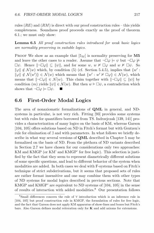
6.5 Standard ND for Weak Logics
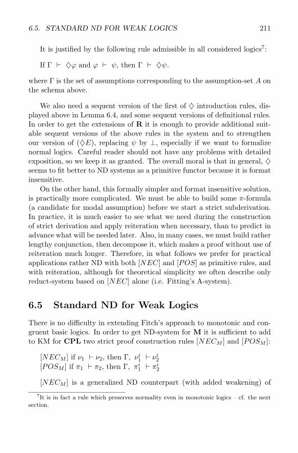
There is no difficulty in extending Fitch’s approach to monotonic and con-gruent basic logics. In order to get ND-system for M it is sufficient to addto KM for CPL two strict proof construction rules [NECM ] and [POSM ]:
[NECM ] if ν1 � ν2, then Γ, νi1 � νi2[POSM ] if π1 � π2, then Γ, πi1 � πi2
[NECM ] is a generalized ND counterpart (with added weakening) of
7It is in fact a rule which preserves normality even in monotonic logics – cf. the nextsection.
212 CHAPTER 6. STANDARD APPROACH TO MODAL LOGICS
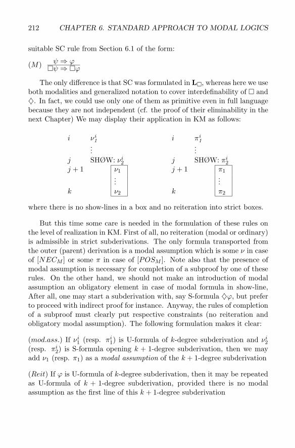
suitable SC rule from Section 6.1 of the form:
(M) ψ ⇒ ϕ�ψ ⇒ �ϕ
The only difference is that SC was formulated in L�, whereas here we useboth modalities and generalized notation to cover interdefinability of � and♦. In fact, we could use only one of them as primitive even in full languagebecause they are not independent (cf. the proof of their eliminability in thenext Chapter) We may display their application in KM as follows:
i νi1 i πi
1...
...j SHØW: νi2 j SHØW: πi2j + 1 ν1 j + 1 π1
......
k ν2 k π2
where there is no show-lines in a box and no reiteration into strict boxes.
But this time some care is needed in the formulation of these rules onthe level of realization in KM. First of all, no reiteration (modal or ordinary)is admissible in strict subderivations. The only formula transported fromthe outer (parent) derivation is a modal assumption which is some ν in caseof [NECM ] or some π in case of [POSM ]. Note also that the presence ofmodal assumption is necessary for completion of a subproof by one of theserules. On the other hand, we should not make an introduction of modalassumption an obligatory element in case of modal formula in show-line,After all, one may start a subderivation with, say S-formula ♦ϕ, but preferto proceed with indirect proof for instance. Anyway, the rules of completionof a subproof must clearly put respective constraints (no reiteration andobligatory modal assumption). The following formulation makes it clear:
(mod.ass.) If νi1 (resp. πi1) is U-formula of k-degree subderivation and νi2(resp. πi2) is S-formula opening k + 1-degree subderivation, then we mayadd ν1 (resp. π1) as a modal assumption of the k + 1-degree subderivation
(Reit) If ϕ is U-formula of k-degree subderivation, then it may be repeatedas U-formula of k + 1-degree subderivation, provided there is no modalassumption as the first line of this k + 1-degree subderivation
6.5. STANDARD ND FOR WEAK LOGICS 213
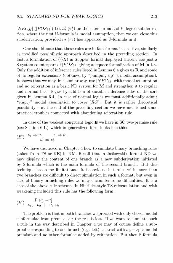
[NECM ] ([POSM ]) Let νi2 (πi2) be the show-formula of k-degree subderiva-tion, where the first U-formula is modal assumption, then we can close thissubderivation, provided ν2 (π2) has appeared as U-formula in it.
One should note that these rules are in fact format-insensitive, similarlyas modified possibilistic approach described in the preceding section. Infact, a formulation of (♦E) in Suppes’ format displayed therein was just aS-system counterpart of [POSM ] giving adequate formalization of M in L♦.Only the addition of inference rules listed in Lemma 6.4 gives us R and someof its regular extensions (obtained by “pumping up” a modal assumption).It shows that we may, in a similar way, use [NECM ] with modal assumptionand no reiteration as a basic ND system for M and strengthen it to regularand normal basic logics by addition of suitable inference rules of the sortgiven in Lemma 6.4. In case of normal logics we must additionally admit“empty” modal assumption to cover (RG). But it is rather theoreticalpossibility – at the end of the preceding section we have mentioned somepractical troubles connected with abandoning reiteration rule.
In case of the weakest congruent logic E we have in SC two-premise rule(see Section 6.1.) which in generalized form looks like this:
(E′) ν1 ⇒ ν2 ν2 ⇒ ν1
νi1 ⇒ νi2
We have discussed in Chapter 4 how to simulate binary branching rules(taken from TS or KE) in KM. Recall that in Jaskowski’s format ND wemay display the content of one branch as a new subderivation initiatedby S-formula which is the main formula of the second branch. But thistechnique has some limitations. It is obvious that rules with more thantwo branches are difficult to direct simulation in such a format, but even incase of binary-branching rules we may encounter some difficulties. It is acase of the above rule schema. In Hintikka-style TS reformulation and withweakening included this rule has the following form:
(E′) Γ, νi1,−νi2ν1,−ν2 | −ν1, ν2
The problem is that in both branches we proceed with only chosen modalsubformulae from premise-set; the rest is lost. If we want to simulate sucha rule in the way described in Chapter 4 we may of course define a sub-proof corresponding to one branch (e.g. left) as strict with ν1,−ν2 as modalpremises and no other formulae added by reiteration. But then S-formula
214 CHAPTER 6. STANDARD APPROACH TO MODAL LOGICS
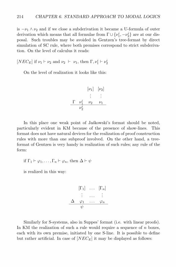
is −ν1 ∧ ν2 and if we close a subderivation it became a U-formula of outerderivation which means that all formulae from Γ∪ {νi1,−νi2} are at our dis-posal. Such troubles may be avoided in Gentzen’s tree-format by directsimulation of SC rule, where both premises correspond to strict subderiva-tion. On the level of calculus it reads:
[NECE ] if ν1 � ν2 and ν2 � ν1, then Γ, νi1 � νi2
On the level of realization it looks like this:
[ν1] [ν2]...
...Γ νi1 ν2 ν1
νi2
In this place one weak point of Jaskowski’s format should be noted,particularly evident in KM because of the presence of show-lines. Thisformat does not have natural devices for the realization of proof constructionrules with more than one subproof involved. On the other hand, a tree-format of Gentzen is very handy in realization of such rules; any rule of theform:
if Γ1 � ϕ1, . . . ,Γn � ϕn, then Δ � ψ
is realized in this way:
[Γ1] . . . [Γn]... . . .
...Δ ϕ1 . . . ϕn
ψ
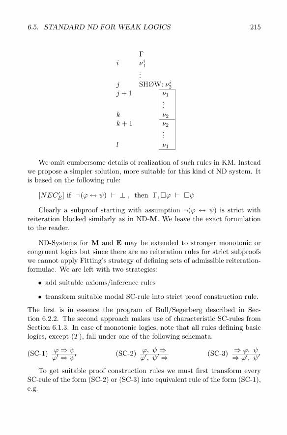
Similarly for S-systems, also in Suppes’ format (i.e. with linear proofs).In KM the realization of such a rule would require a sequence of n boxes,each with its own premise, initiated by one S-line. It is possible to definebut rather artificial. In case of [NECE ] it may be displayed as follows:
6.5. STANDARD ND FOR WEAK LOGICS 215
Γi νi
1...
j SHØW: νi2j + 1 ν1
...k ν2
k + 1 ν2...
l ν1
We omit cumbersome details of realization of such rules in KM. Insteadwe propose a simpler solution, more suitable for this kind of ND system. Itis based on the following rule:
[NEC ′E ] if ¬(ϕ↔ ψ) � ⊥ , then Γ,�ϕ � �ψ
Clearly a subproof starting with assumption ¬(ϕ ↔ ψ) is strict withreiteration blocked similarly as in ND-M. We leave the exact formulationto the reader.
ND-Systems for M and E may be extended to stronger monotonic orcongruent logics but since there are no reiteration rules for strict subproofswe cannot apply Fitting’s strategy of defining sets of admissible reiteration-formulae. We are left with two strategies:
• add suitable axioms/inference rules
• transform suitable modal SC-rule into strict proof construction rule.
The first is in essence the program of Bull/Segerberg described in Sec-tion 6.2.2. The second approach makes use of characteristic SC-rules fromSection 6.1.3. In case of monotonic logics, note that all rules defining basiclogics, except (T ), fall under one of the following schemata:
(SC-1) ϕ⇒ ψϕ′ ⇒ ψ′ (SC-2) ϕ, ψ ⇒
ϕ′, ψ′ ⇒ (SC-3) ⇒ ϕ, ψ⇒ ϕ′, ψ′
To get suitable proof construction rules we must first transform everySC-rule of the form (SC-2) or (SC-3) into equivalent rule of the form (SC-1),e.g.
216 CHAPTER 6. STANDARD APPROACH TO MODAL LOGICS
(5) ⇒ �ϕ,ψ⇒ �ϕ,�ψ
is transformed into:
(5’) ¬�ϕ⇒ ψ¬�ϕ⇒ �ψ
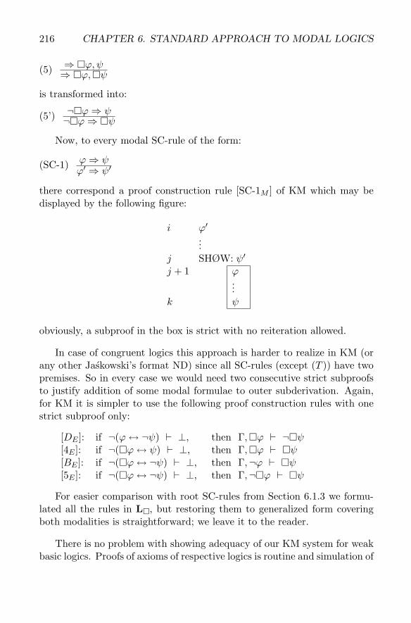
Now, to every modal SC-rule of the form:
(SC-1) ϕ⇒ ψϕ′ ⇒ ψ′
there correspond a proof construction rule [SC-1M ] of KM which may bedisplayed by the following figure:
i ϕ′...
j SHØW: ψ′
j + 1 ϕ...
k ψ
obviously, a subproof in the box is strict with no reiteration allowed.
In case of congruent logics this approach is harder to realize in KM (orany other Jaskowski’s format ND) since all SC-rules (except (T )) have twopremises. So in every case we would need two consecutive strict subproofsto justify addition of some modal formulae to outer subderivation. Again,for KM it is simpler to use the following proof construction rules with onestrict subproof only:
[DE ]: if ¬(ϕ↔ ¬ψ) � ⊥, then Γ,�ϕ � ¬�ψ[4E ]: if ¬(�ϕ↔ ψ) � ⊥, then Γ,�ϕ � �ψ[BE ]: if ¬(�ϕ↔ ¬ψ) � ⊥, then Γ,¬ϕ � �ψ[5E ]: if ¬(�ϕ↔ ¬ψ) � ⊥, then Γ,¬�ϕ � �ψ
For easier comparison with root SC-rules from Section 6.1.3 we formu-lated all the rules in L�, but restoring them to generalized form coveringboth modalities is straightforward; we leave it to the reader.
There is no problem with showing adequacy of our KM system for weakbasic logics. Proofs of axioms of respective logics is routine and simulation of
6.6. FIRST-ORDER MODAL LOGICS 217
rules (RE) and (RM) is direct with our proof construction rules – this yieldscompleteness. Soundness proof proceeds exactly as the proof of theorem6.1.; we must only show:
Lemma 6.5 All proof construction rules introduced for weak basic logicsare normality preserving in suitable logics.
Proof We show as an example that [5M ] is normality preserving for M5and leave the other cases to a reader. Assume that ¬�ϕ |= ψ but ¬�ϕ �|=�ψ. Hence ‖¬�ϕ‖ ⊆ ‖ψ‖, and for some w, w � �ϕ and w � �ψ. So‖ϕ‖ /∈ N (w) which, by condition (5) (cf. Section 5.4.5), implies that {w′ :‖ϕ‖ /∈ N (w′)} ∈ N (w) which means that {w′ : w′
� �ϕ} ∈ N (w), whichmeans that ‖¬�ϕ‖ ∈ N (w). This claim together with ‖¬�ϕ‖ ⊆ ‖ψ‖ bycondition (m) yields ‖ψ‖ ∈ N (w). But then w � �ψ, a contradiction whichshows that ¬�ϕ |= �ψ.
6.6 First-Order Modal Logics
The area of nonaxiomatic formalizations of QML in general, and ND-systems in particular, is not very rich. Fitting [93] provides some systemsbut with rules for quantifiers borrowed from TS. Indrzejczak [139, 141] pro-vides a characterization of many logics on the basis of KM, whereas Garson[104, 105] offers solutions based on ND in Fitch’s format but with Gentzen’srule for elimination of ∃ and with parameters. In what follows we briefly de-scribe in what way several versions of QML described in Chapter 5 may beformalized on the basis of ND. From the plethora of ND variants describedin Section 2.7 we have chosen for our considerations only two approaches:KM and KMGP (or KM’ and KMGP’ for free logic). This selection is justi-fied by the fact that they seem to represent diametrically different solutionsof some specific questions, and lead to different behavior of the system whenmodalities are added. In both cases we deal with F-systems based on Fitch’stechnique of strict subderivations, but it seems that proposed sets of rulesare rather format insensitive and one may combine them with other typesof ND systems for modal logics described in previous sections. Note thatKMGP and KMGP’ are equivalent to ND systems of [104, 105] in the senseof results of interaction with added modalities.8 Our presentation follows
8Small differences concern the rule of ∀ introduction which is an inference rule in[104, 105] but proof construction rule in KMGP, the formulation of rules for free logic,and the fact that Garson does not apply KM apparatus of show-lines and boxes but Fitch’sbars. Also Garson defines modal reiteration only for K and add axioms for extensions.
218 CHAPTER 6. STANDARD APPROACH TO MODAL LOGICS
strictly the order introduced in Chapter 5 and applies only to normal logics.
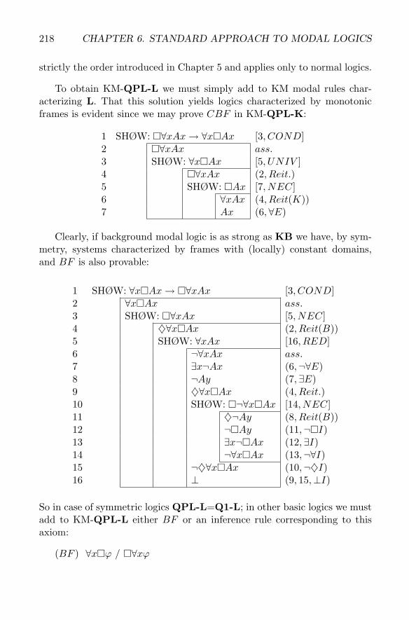
To obtain KM-QPL-L we must simply add to KM modal rules char-acterizing L. That this solution yields logics characterized by monotonicframes is evident since we may prove CBF in KM-QPL-K:
1 SHØW: �∀xAx→ ∀x�Ax [3, COND]2 �∀xAx ass.3 SHØW: ∀x�Ax [5, UNIV ]4 �∀xAx (2, Reit.)5 SHØW: �Ax [7, NEC]6 ∀xAx (4, Reit(K))7 Ax (6,∀E)
Clearly, if background modal logic is as strong as KB we have, by sym-metry, systems characterized by frames with (locally) constant domains,and BF is also provable:
1 SHØW: ∀x�Ax→ �∀xAx [3, COND]2 ∀x�Ax ass.3 SHØW: �∀xAx [5, NEC]4 ♦∀x�Ax (2, Reit(B))5 SHØW: ∀xAx [16, RED]6 ¬∀xAx ass.7 ∃x¬Ax (6,¬∀E)8 ¬Ay (7,∃E)9 ♦∀x�Ax (4, Reit.)10 SHØW: �¬∀x�Ax [14, NEC]11 ♦¬Ay (8, Reit(B))12 ¬�Ay (11,¬�I)13 ∃x¬�Ax (12,∃I)14 ¬∀x�Ax (13,¬∀I)15 ¬♦∀x�Ax (10,¬♦I)16 ⊥ (9, 15,⊥I)
So in case of symmetric logics QPL-L=Q1-L; in other basic logics we mustadd to KM-QPL-L either BF or an inference rule corresponding to thisaxiom:
(BF ) ∀x�ϕ / �∀xϕ
6.6. FIRST-ORDER MODAL LOGICS 219
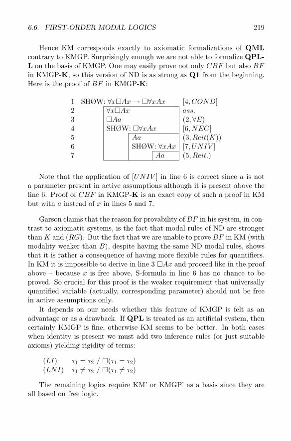
Hence KM corresponds exactly to axiomatic formalizations of QMLcontrary to KMGP. Surprisingly enough we are not able to formalize QPL-L on the basis of KMGP. One may easily prove not only CBF but also BFin KMGP-K, so this version of ND is as strong as Q1 from the beginning.Here is the proof of BF in KMGP-K:
1 SHØW: ∀x�Ax→ �∀xAx [4, COND]2 ∀x�Ax ass.3 �Aa (2,∀E)4 SHØW: �∀xAx [6, NEC]5 Aa (3, Reit(K))6 SHØW: ∀xAx [7, UNIV ]7 Aa (5, Reit.)
Note that the application of [UNIV ] in line 6 is correct since a is nota parameter present in active assumptions although it is present above theline 6. Proof of CBF in KMGP-K is an exact copy of such a proof in KMbut with a instead of x in lines 5 and 7.
Garson claims that the reason for provability of BF in his system, in con-trast to axiomatic systems, is the fact that modal rules of ND are strongerthan K and (RG). But the fact that we are unable to prove BF in KM (withmodality weaker than B), despite having the same ND modal rules, showsthat it is rather a consequence of having more flexible rules for quantifiers.In KM it is impossible to derive in line 3 �Ax and proceed like in the proofabove – because x is free above, S-formula in line 6 has no chance to beproved. So crucial for this proof is the weaker requirement that universallyquantified variable (actually, corresponding parameter) should not be freein active assumptions only.
It depends on our needs whether this feature of KMGP is felt as anadvantage or as a drawback. If QPL is treated as an artificial system, thencertainly KMGP is fine, otherwise KM seems to be better. In both caseswhen identity is present we must add two inference rules (or just suitableaxioms) yielding rigidity of terms:
(LI) τ1 = τ2 / �(τ1 = τ2)(LNI) τ1 �= τ2 / �(τ1 �= τ2)
The remaining logics require KM’ or KMGP’ as a basis since they areall based on free logic.
220 CHAPTER 6. STANDARD APPROACH TO MODAL LOGICS
ND-QS-L is obtained by a combination of KM’ or KMGP’ with modalrules QPL-L for suitable L. Similarly we obtain ND for G-L but withsuitable restrictions, both (F∀E) and (F∃I) must be weakened: in KM’only variables, and in KMGP’ only parameters may be values of τ . Thelogic F-L is obtainable just like G-L but E is counted as atomic. Finally,Q1R-L without identity is just like QS-L, otherwise we must add (LI) and(LNI); Eτ is counted as atomic.
In case of Q3-L we proceed as in case of G-L but in axiomatic formula-tion also rules (G∀E), (G∀I) and (G = E) were needed. In this respect NDformulations behave better in general but KMGP’ is the winer. Both gen-eralized rules for ∀ are derivable in KMGP’, whereas in KM’ only the firstof them. We must add (G∀I) as a primitive rule to KM’-Q3-L althoughsuch a solution is artificial. In contrast to KMGP’, in KM’ it cannot beproved because of the similar reasons as with unprovability of BF in KMand provability in KMGP. To secure completeness (G = E) must be addedto both ND systems for Q3-L but it may be simplified:
(G = E)′ � ϕ→ x �= τ / � ϕ→ ⊥
where x /∈ V F ({ϕ, τ})
It is easy to show that (G = E) is provable in KM’ (or KMGP’) with(G = E)′.
Completeness of these ND systems follows easily from completeness ofrespective ND systems for first-order logics and for propositional modal log-ics. Soundness may be proved by combination of suitable proof for proposi-tional modal logics with the result for ND systems for first-order logics fromChapter 2. Clearly in case of KM or KM’ we must first make a transfor-mation into KMG or KMG’ (cf. Chapter 2) but note that the presence of[NEC] or [POS] does not harm to the proof of Lemma 2.3. We encouragethe reader to repeat soundness proof from Section 6.4.2 for various systemsenriched with rules for quantifiers.