natural bayesian killers -...

Natural Bayesian Killers

Team #8215

February 22, 2010

Abstract

In criminology, the real life CSI currently faces an interestingphase, where mathematicians are entering the cold-blooded field offorensics. Geographic profiling uses existing geocoded data to pre-dict, solve and prevent crime. In this study, we examine probabilitydistance strategies and a Bayesian approach used to predict the res-idential location of a serial offender. We compare different distancedecay functions used for estimating the probability density of theresidential location. Additionally, we derive a Bayesian approach forpredicting the next target location of the serial offender followingthe formulation of O’Leary [2009].

For the measure of performance, we choose the search cost rank-ing. The model is tested using the leave-one-out cross-validation witha small example dataset that consists of serial murder cases. Differ-ent strategies of combining the six different methods are discussed.The tests suggest that the best predictions are achieved using theBayesian approach with exponential decay function. However, thisresult is not statistically significant due to the lack of test data.

Team number: #8215 of 27

Contents

1 Introduction 3

2 Predicting the Residential Location of the Offender 5

2.1 Spatial Distribution Strategies . . . . . . . . . . . . . . . . . . 5

2.2 Probability Distance Strategies . . . . . . . . . . . . . . . . . 5

2.2.1 Distance Decay Functions . . . . . . . . . . . . . . . . 6

2.3 A Bayesian Approach . . . . . . . . . . . . . . . . . . . . . . . 9

2.3.1 Assumptions . . . . . . . . . . . . . . . . . . . . . . . 10

2.3.2 Normalization . . . . . . . . . . . . . . . . . . . . . . . 11

2.3.3 Performance of the Prediction . . . . . . . . . . . . . 11

2.4 Combining Models . . . . . . . . . . . . . . . . . . . . . . . . 13

3 Predicting the Next Target Location 14

3.1 A Bayesian Approach . . . . . . . . . . . . . . . . . . . . . . . 14

3.2 Assumptions . . . . . . . . . . . . . . . . . . . . . . . . . . . . 15

3.3 Performance of the Prediction . . . . . . . . . . . . . . . . . . 16

4 Experiments 17

4.1 Data . . . . . . . . . . . . . . . . . . . . . . . . . . . . . . . . . 17

4.2 Calibration and Validation . . . . . . . . . . . . . . . . . . . . 18

5 Results 19

5.1 Sensitivity Analysis . . . . . . . . . . . . . . . . . . . . . . . . 23

6 Conclusions 25

Appendix A: Technical Summary for a Crime Investigator


1 Introduction

For the untrained eye, a set of crime sites of a serial killer might seemtotally random when visualized on a map. However, the behavior of theserial killer usually has some underlying statistical regularities which canbe discovered by computerized data analysis. The same sort of behaviorcan be found for all kinds of serial offenders: killers, rapists, burglars, etc.This type of analysis is called geographic profiling.

Understanding the statistical regularities may help predicting the offender’sanchor point (residence, workplace, etc.). This can be crucial for catch-ing the offender before further crimes are committed. However, the ge-ographic profiling methods usually neglect some essential pieces of in-formation regarding the situation, such as that it is very unlikely to findthe offender’s residence from the middle of a lake. Therefore, geographicprofiling should be considered a decision support system rather than anexpert system [Canter et al., 2000].

In Section 2, we first present the spatial distribution strategies which are asimple approach to the problem [Snook et al., 2005]. They predict the of-fender’s anchor point by calculating, e.g., the centroid of the crime sites.Another category of strategies is the probability distribution strategies whichare the most common way of addressing the problem of finding the an-chor point. They rely on distance decay functions, which estimate the dis-tribution of the distances the offender is willing to travel to the crime site.Several studies that compare different decay functions exist [Levine, 2004,Canter and Hammond, 2006, Snook et al., 2005].

In recent years, there has been a rise in the popularity of the Bayesianapproaches tackling the problem of locating the anchor point. This can beseen in the number of papers published recently [O’Leary, 2009, Mohlerand Short, 2009, Levine, 2009]. Following O’Leary [2009], we derive theprobability density function (PDF) for the anchor point from the Bayes’rule. We then discuss the assumptions behind the Bayesian formalismand also address the question, how to measure the performance of theprediction.

At the end of Section 2, we present methods for combining the predictionsof different methods. The most advanced combination methods can takethe different strengths of different models into account.


A crime investigator might also be interested in knowing the next targetof the offender. Section 3 deals with this problem presenting a Bayesianapproach for estimating the PDF of the next crime site. O’Leary [2009]shows how this approach comes almost free of charge after we have de-rived the PDF for the anchor point.

Section 4 discusses the data used for testing the geographic profilingmethods. It also describes the leave-one-out cross-validation method, whichis a useful method for small data samples.

In Section 5 we present the results and some sensitivity analysis. Afterdrawing the conclusions in Section 6, we give a technical summary thatdescribes how a crime investigator can utilize the Bayesian approach forlocating the offender’s anchor point and the next target location.


2 Predicting the Residential Location of the Of-fender

Geographic profiling is used as a decision support system for locatingthe anchor point (residence, workplace, etc.) of a serial offender [Canteret al., 2000]. A prediction for the anchor point is given based on the of-fender’s crime site locations. The prediction can be either a single spotor a probability density. This criteria divides the prediction methods intospatial distribution strategies and probability distance strategies [Snook et al.,2005].

2.1 Spatial Distribution Strategies

Spatial distribution strategies calculate a central point of the crime sitelocations. This point is an estimate of the anchor point. Various methodsfor calculating the central point have been proposed. Snook et al. [2005]compare 6 different spatial distribution strategies: centroid, centre of thecircle, median, geometric mean, harmonic mean and center of minimum distance.

The centroid method is the simplest of these strategies and it calculatesthe mean of the x and y coordinates. Even this simple method can pro-vide useful predictions, as in the case of the ”Yorkshire Ripper” wherethe method was able to predict correctly the killer’s home town. Further-more, Snook et al. [2005] suggest that complexity of the strategy does notguarantee a better accuracy.

A restraint of the spatial distribution strategies is that they only providea single point as the prediction. If the offender is not found there, the sys-tem does not give any advice for the crime investigator where to continuethe search.

2.2 Probability Distance Strategies

Probability distance strategies (PDS), also referred as journey-to-crime esti-mation [Levine, 2004], create a geographical profile which is usually dis-played on a map. The height of the profile indicates the likelihood of theanchor point to be found on the corresponding place. Thus, PDS provide


a prioritized search strategy which can give them a significant advantageover the spatial distribution strategies [Snook et al., 2005].

PDS are based on distance decay functions that characterize the distribu-tion of distances between the anchor point and the crime scenes. Com-parison of different decay functions has been conducted by Levine [2004],Canter and Hammond [2006] and Snook et al. [2005]. Popular decay func-tions are: negative exponential, lognormal, normal, truncated negative exponen-tial, and linear functions.

To create the geographical profile, we discretize the search area and gothrough each point y. We calculate the overall effect of all the crime sitesxi on y and get the hit score S(y) as referred by O’Leary [2009]

S(y) =n

∑i=1

f (d(xi, y)) = f (d(x1, y)) + · · ·+ f (d(xn, y)). (1)

The distance function d can be selected, e.g., as the Euclidean or the Man-hattan distance. In our analysis, we use the Euclidean distance. The hitscore gives a priority order to the search. Figure 1 shows an exampleof a geographic profile regarding the case of serial killer Peter Sutcliffe,the Yorkshire Ripper. Crime sites are marked with red circles and Sut-cliffe’s residence with a black circle. The centroid point of the crime sitesis marked with a black cross.

A red value in the profile denotes a good chance of finding the anchorpoint. We can see that the actual location of the residence — the anchorpoint — is clearly in the red zone of the map, but the peak of the profileis located somewhat away from the anchor point.

2.2.1 Distance Decay Functions

Distribution of the distances between the anchor point and the crimescenes is characterized by a distance decay function [Canter and Ham-mond, 2006]. Common choices for the decay function include: negative ex-ponential, lognormal, normal, truncated negative exponential, and linear func-tions. Comparison of different decay functions has been conducted byLevine [2004], Canter and Hammond [2006] and Snook et al. [2005].


Figure 1: A geographic profile regarding the case of serial killer Peter Sut-cliffe, the Yorkshire Ripper. Crime sites are marked with red circles andSutcliffe’s residential location with a black circle. The centroid point of thecrime sites is marked with a black cross.

Decay functions usually give high values for low distances, i.e. the of-fender is not willing to travel far to commit the crime. Lognormal andtruncated negative exponential functions also implement a buffer zonewhich corresponds to the behavior that the offender might not feel com-fortable committing a crime right next to their residence.

In this paper, we study three different decay functions: lognormal, neg-ative exponential and gamma functions. All three are continuous anddifferentiable probability density functions


fLogN(d; µ, σ) =1

xσ√

2πe−

(ln x−µ)2

2σ2 , (2)

fExp(d; λ) = λe−λx, (3)

fGamma(d; µ, σ) = xk−1 e−x/θ

θkΓ(k). (4)

The gamma distribution is chosen since the exponential distribution is aspecial case of it where k = 1. However, by increasing the k parameter abuffer zone is created.

In Figure 2 we see the three decay functions fitted to real data.

0 1 2 3 4 5 6 7 80

0.2

0.4

0.6

0.8

Normalized distance

Pro

bab

ilit

y d

ensi

ty

Histogram

LogN

Gamma

Exp

Figure 2: A histogram of normalized distances and the three different decayfunctions that have been fitted to the data.

The parameters of the decay function are estimated using the maximumlikelihood estimation [Alpaydin, 2004, p. 62]. The advantage of this methodis that it gives confidence intervals for the parameters, which allow us toassess the uncertainty in the predictions.


2.3 A Bayesian Approach

O’Leary [2009] applies the Bayes’ rule to derive the probability distri-bution P(z|x1, . . . , xn) for the anchor point z based on the crime sitesx1, . . . , xn

1.

The Bayes’ rule gives us

P(z|x1, . . . , xn) =P(x1, . . . , xn|z)P(z)

P(x1, . . . , xn). (5)

The prior probability density function P(z) is set to the constant value 1in our analysis. However, it could be straightforwardly included in orderto take the geographic properties of the search area into account. Forexample, we could define

P(z) =

{0 , when z ∈ uninhabitable areas1 , when z /∈ uninhabitable areas

(6)

to exclude the uninhabitable from the search. Mohler and Short [2009]have used this approach and merged the housing density into P(z).

P(x1, . . . , xn) in Formula (5) can be ignored, since it is merely a scalingfactor that is independent of the anchor point z. Assuming that the crimesites are statistically independent, we get

P(x1, . . . , xn|z) = P(x1|z) · · · P(xn|z). (7)

Thus we may write

P(z|x1, . . . , xn) ∝ P(x1|z) · · · P(xn|z). (8)

The term P(x1|z) depends on the distance decay function f (d) and theprior probability density function of the crime sites P(x). The offendermight be prone to commit crimes, e.g., in the less populated areas. This

1O’Leary also includes an α parameter which defines the shape of the offender’sdistance decay function. However, we assume that the same shape parameters hold forall offenders. We normalize the distances in order to take into account the individualscales of the crime site distributions.


behavior could be encoded in P(x). In our analysis, we restrict our focusto the case P(x) = 1, and thus we get

P(xi|z) = f (d(xi, z)) (9)

and finally

P(z|x1, . . . , xn) ∝ f (d(x1, z)) · · · f (d(xn, z)). (10)

We notice that without the priors P(z) and P(x), we get almost the sameformula that is traditionally used (1). Only the summation is replaced bymultiplication.

The advantage of the Bayesian approach is that it is mathematically well-founded given the assumptions it makes (see Section 2.3.1). It also pro-vides a natural way to include information about geographical propertiesof the area (e.g., by excluding uninhabitable areas from the search area).

2.3.1 Assumptions

The Bayesian approach makes the following assumptions

1. Independent crime sites: P(x1, . . . , xn|z) = P(x1|z) · · · P(xn|z)

The offender chooses the next crime site regardless of the previouscrime sites. This assumption is also made by O’Leary [2009] andMohler and Short [2009].

2. Distance decay function parameters are the same for all offenders

Warren et al. [1998] suggest that the distance travelled by a serialrapist depends on the age and race of the rapist. To take this intoaccount, our model normalizes all distances by the mean inter-pointdistances, as done by Canter et al. [2000]. However, Warren et al.[1998] also suggest that the more rapes there are on the rapist’saccount, the farther the rapist tends to travel. Our model ignoresthis possibility.

3. Uniform anchor point distribution: P(z) = 1


Our analyses have been conducted giving the same prior probabilityto all locations. This ignores the geographical properties, such asuninhabitable areas and housing densities, which naturally affectthe distribution. However, these properties could be easily includedin our model, if there was access to relevant data of the search area.

4. Uniform crime site distribution: P(x) = 1

We do not make any prior assumptions of the crime site distribu-tion. We reckon that for example for sexual offences very publicplaces are not as probable crime sites as more private ones. Again,this information can be included in our model if the data is avail-able.

2.3.2 Normalization

The average distance an offender is willing to travel to commit a crimevaries between individuals. Warren et al. [1998] suggest that these indi-vidual differences can be explained by variables such as the offender’sage and race.

Canter et al. [2000] describe two normalization methods for taking theindividual differences into account. The first method calculates the meaninter-point distance (MID) between all offenses. When estimating the de-cay function parameters or applying the decay function in Formula (10),the distances are always normalized by dividing them by the MID.

The second method, called the QRange, calculates a linear regression ofthe crime sites. Instead of the MID, the perpendicular distance from ev-ery crime site to the regression line is calculated. This method takes intoaccount any linear structure in the crime site distribution which mightderive, e.g., from an arterial pathway.

In our analysis, the normalization is conducted with the MID metric.

2.3.3 Performance of the Prediction

To compare a variety of methods, we need a way to measure the effec-tiveness of different techniques. Canter et al. [2000] propose that reducingpolice resources would be a suitable objective. The potential search area


is discretized to a grid. The cost of carrying out a search on a particularspot (or cell in the grid) depends on the number of searched cells before.The assumption is that the police start the search at the most probablespot and move from spot to spot by decreasing probability.

Different decay functions can this way be compared by their cost-effectivity.This measure reflects the ability of a method to prioritize a cell and iden-tify the location of the anchor point. A search area is estimated by calcu-lating the mean inter-point distance, in a Manhattan sense, between crimesites with respect to the x coordinates

xm =1

n(n− 1)

n

∑i=1

n

∑j=1|xi − xj|. (11)

and y coordinates

ym =1

n(n− 1)

n

∑i=1

n

∑j=1|yi − yj|. (12)

separately. Rossmo [1995a] introduces the concept of a rectangular searcharea — also called the hunting area. The rectangle is fitted to the farthestextent of the known linked crime sites, and it is extended by half of themean Manhattan distance xm on the horizontal axis and half the ym onthe vertical axis in all directions. We use this approach, but we extend thesearch area by the mean value in every direction, i.e. by 2xm horizontallyand 2ym vertically.

The effectiveness of the search of the rectangular area is calculated byassigning each point on the grid a weighting indicating the likelihood ofresidence. Canter et al. [2000] use this method so that the weightings areused to calculate a search cost rank index for each grid cell. These searchcost rank indexes are derived from the decay function that the methoduses.

Each cell point inside the array is then searched for the anchor point, start-ing from the highest rank index. When the anchor point cell is reached,the search is terminated and a search cost value is calculated. This valuereflects the proportion of the rectangle that has been searched before ter-mination. A search cost value of 0 would indicate that the criminal was


found in the first cell (i.e. the cell with the highest priority). If the searchis terminated without reaching the known location of the criminal, theanchor point was not within the search area. This means that the methodwas a failure.

2.4 Combining Models

Different decay functions give different geographical profiles. Calculatingan ensemble of these profiles can make the predictions more accurate andmore stable. Finding the underlying profile can be seen as a regressionproblem and thus, we have a regression ensemble problem, as referred inthe machine learning community.

Alpaydin [2004] shows several simple strategies for calculating the en-semble, two of which are the average and median strategies. The aver-age strategy iterates over the search area and at each point it calculatesthe average height of the profiles given by different models. The medianstrategy takes the median of the heights. According to Alpaydin [2004],the sum strategy is the most widely used in practice. The advantage ofthe median strategy is that it is more robust to outliers.

Several studies about more advanced regression ensemble methods ex-ist (see e.g. Brown et al. [2005]; Ratsch et al. [2002]). The more advancedmethods take into account the strengths and weaknesses of different mod-els. For example, one method can give more accurate predictions in thecases where the mean inter-point distance (MID) of the offences is high,whereas another one is more suitable for cases with a low MID.

A straightforward strategy for exploiting the different strengths of themodels is to divide the range of the MID values into n intervals. For eachinterval, we calculate which model gives the best results for the caseswithin that interval. When we get a new case, we calculate the new MID,and then check which interval the new MID goes into and let the bestmodel within that interval calculate the geographic profile.

In our case, the decay functions tested did not give statistically differentresults due to limited amount of test data. Therefore, no ensemble meth-ods were tested in our study. To adapt the models to different types ofoffenders, bagging or boosting methods could be adopted, as describedin [Alpaydin, 2004, pp. 430–434].


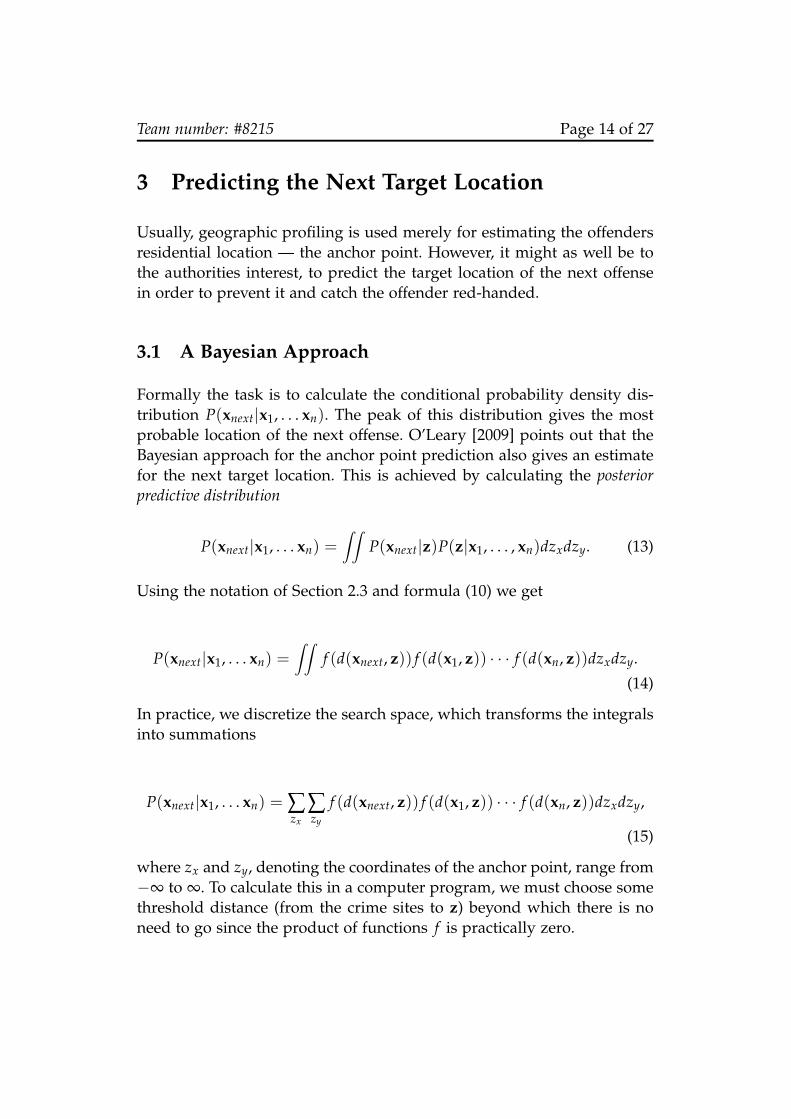
3 Predicting the Next Target Location

Usually, geographic profiling is used merely for estimating the offendersresidential location — the anchor point. However, it might as well be tothe authorities interest, to predict the target location of the next offensein order to prevent it and catch the offender red-handed.

3.1 A Bayesian Approach

Formally the task is to calculate the conditional probability density dis-tribution P(xnext|x1, . . . xn). The peak of this distribution gives the mostprobable location of the next offense. O’Leary [2009] points out that theBayesian approach for the anchor point prediction also gives an estimatefor the next target location. This is achieved by calculating the posteriorpredictive distribution

P(xnext|x1, . . . xn) =∫∫

P(xnext|z)P(z|x1, . . . , xn)dzxdzy. (13)

Using the notation of Section 2.3 and formula (10) we get

P(xnext|x1, . . . xn) =∫∫

f (d(xnext, z)) f (d(x1, z)) · · · f (d(xn, z))dzxdzy.

(14)

In practice, we discretize the search space, which transforms the integralsinto summations

P(xnext|x1, . . . xn) = ∑zx

∑zy

f (d(xnext, z)) f (d(x1, z)) · · · f (d(xn, z))dzxdzy,

(15)

where zx and zy, denoting the coordinates of the anchor point, range from−∞ to ∞. To calculate this in a computer program, we must choose somethreshold distance (from the crime sites to z) beyond which there is noneed to go since the product of functions f is practically zero.


Figure 3 shows an example of the next target’s estimated probability den-sity function based on the previous offenses. The figure is read similarlyto the geographical profiles, i.e. the next target is likely to be found in thered area.

Figure 3: A profile of the next target of Peter Sutcliffe. Crime sites are markedwith red circles and Sutcliffe’s residential location with a black circle. A redvalue indicates high probability density.

3.2 Assumptions

We make the same assumptions that were presented and discussed inSection 2.3.1. Again, we assume that the offenses are statistically inde-pendent meaning that the predictions are invariant to the order — andtime — of the offenses.


3.3 Performance of the Prediction

The search cost approach, described in Section 2.3.3, can be utilized in thiscase with some minor modifications. Instead of calculating the search costof the anchor point, we calculate it for some of the previous crime sites.This crime site is left out from the calibration phase.

Calculating the profile for the next target is very similar to calculating thegeographic profile for the anchor point. However, the time complexitygrows from O(n) to O(n2), where n is the number of cells in the grid. Inconsequence, calculating the next target profile takes approximately onehour with a 100x100 grid on an average desktop computer.


4 Experiments

4.1 Data

Both the spatial distribution strategies and the probability distance strate-gies described earlier are applicable to any data series of activity that in-cludes geographical locations. Snook et al. [2005], Gorr [2004], Rossmo[1995b] and many more have used sample datasets of solved serial crimeto validate and test their models. Most of these datasets are either classi-fied or kept out of public for some other reason.

Our small test dataset consists of six cases of serial crime, some of whichhave gained notable public attention. These datasets are used for param-eter estimation and cross validation of the models. The cases included arenamed after convicted criminals, which are Peter “The Yorkshire Ripper”Sutcliffe [Wikipedia], Chester Turner [Iniguez, L.], Gary “Green RiverKiller” Ridgway [Nowlin M. and Chaumont K., 2003], John Allen “theBeltway Sniper” Muhammad [Wikipedia, 2010], Steve “the Suffolk Stran-gler” Wright [Harris, 2008] and Terry Blair [News, 2004]. These cases areshortly introduced in table 1. In addition to the location data regardingvictims, also a residential home location (an anchor point) of the convictwas part of every case.

Table 1: The six cases of serial murder used for validating and testing.

Dataset Name of Criminal Datapoints Years active Country

Sutcliffe2 Peter Sutcliffe 18 1975-80 UKTurner Chester Turner 12 1987–98 USRidgway Gary Ridgway 30 1982–90 USMuhammad3 John Allen Muhammad 15 2002 USWright Steve Wright 5 2006 UKBlair Terry Blair 5 2004 US

2The dataset Sutcliffe includes four datapoints of attempted murder.3In the Muhammad set, the home location is specified by the place of arrest, due to

the fact that Muhammad lived in his van.


4.2 Calibration and Validation

We use datasets from table 1 to get a number of training and validation setpairs. The purpose is to train the method using a dataset X (after havingleft out some part as the test set). The small dataset limits the effective useof this method. Repeated use of the same data split differently correctssome drawback. This method is called cross-validation. In K-fold cross-validation, the dataset X is divided randomly into K equal-sized parts,Xi, i = 1, ..., K. To generate the pairs, we keep one of the K parts out asthe validation set and use the remaining K − 1 parts as the training set.Doing this K times — each time leaving out a different part — we get Kparts. [Alpaydin, 2004, pp-486-7]

With a small dataset the only practical option is the extreme case of K-fold cross-validation called leave-one-out, where only one part is left outas the validation set and training uses the N − 1 remaining parts. Thisway we get N separate pairs by leaving out a different instance at eachiteration. [Alpaydin, 2004, p. 487]


5 Results

Our approach uses three different decay functions: lognormal, negativeexponential and the gamma function. To compare the results each of de-cay function, we use the cross-validation method of leave-one-out to esti-mate the decay functions’ parameters from five datasets and then predictthe anchor point in the sixth dataset. The results of the different cases arecompared with the help of a [0, 1] scaled search cost estimate, where azero cost is optimal.

In addition to the three different decay functions, we compare the Bayesianapproach (equation 5) and the traditional summation method (equation1).

(a) Bayesian Approach. (b) Summation method.

Figure 4: Predictions for the sutcliffe dataset which has been calibrated withthe other five sets. The search area is marked with a dotted rectangle. Crimesites are marked with red circles, the location of residence with a black circle,and the center of mass is marked with a black cross.

Figure 4(a) shows the search cost on a map with the help of a color map.The more red a particular spot, the better the search cost. The dottedrectangle depicts the search area. Crime sites are marked with red circles,the location of residence with a black circle, and the centroid spot, “thecenter of mass”, is marked with a black cross. To clarify the effect of risingsearch costs some contour lines are shown on the map.


Figure 4(a) uses the lognormal decay function and the Bayesian approach.Figure 4(b) uses the summation method. Differences between these twomethods are marginal, although the coloring varies. By calculating thesearch cost rank index, we are only interested in the order of the cell list(See Section 2.3.3). The effect of the lognormal buffer zone can be seen asholes around the crime sites.

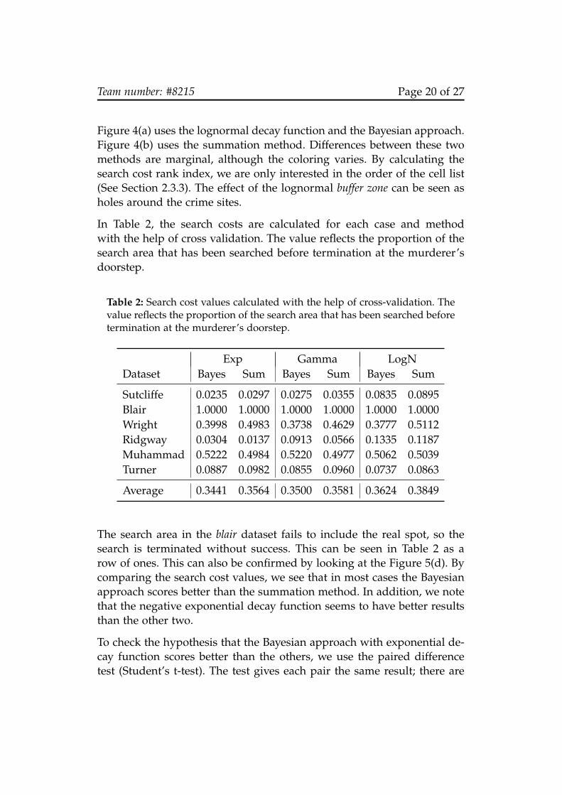
In Table 2, the search costs are calculated for each case and methodwith the help of cross validation. The value reflects the proportion of thesearch area that has been searched before termination at the murderer’sdoorstep.

Table 2: Search cost values calculated with the help of cross-validation. Thevalue reflects the proportion of the search area that has been searched beforetermination at the murderer’s doorstep.

Exp Gamma LogNDataset Bayes Sum Bayes Sum Bayes Sum

Sutcliffe 0.0235 0.0297 0.0275 0.0355 0.0835 0.0895Blair 1.0000 1.0000 1.0000 1.0000 1.0000 1.0000Wright 0.3998 0.4983 0.3738 0.4629 0.3777 0.5112Ridgway 0.0304 0.0137 0.0913 0.0566 0.1335 0.1187Muhammad 0.5222 0.4984 0.5220 0.4977 0.5062 0.5039Turner 0.0887 0.0982 0.0855 0.0960 0.0737 0.0863

Average 0.3441 0.3564 0.3500 0.3581 0.3624 0.3849

The search area in the blair dataset fails to include the real spot, so thesearch is terminated without success. This can be seen in Table 2 as arow of ones. This can also be confirmed by looking at the Figure 5(d). Bycomparing the search cost values, we see that in most cases the Bayesianapproach scores better than the summation method. In addition, we notethat the negative exponential decay function seems to have better resultsthan the other two.

To check the hypothesis that the Bayesian approach with exponential de-cay function scores better than the others, we use the paired differencetest (Student’s t-test). The test gives each pair the same result; there are


no significant differences between the methods in our datasets. The nullhypothesis of equal means is confirmed.

In Figures 5(a) and 5(c) we see the results of the wright and turner datasets.In these two cases the home location of the criminal is consistent withthe predicted anchor point. In addition, we notice that even the centerof mass succeeds well in predicting the location. On the other hand, inFigures 5(b) and 5(d), where we see the results of the muhammad and blairdatasets, the model is not quite successful. In fact — as noted before —the model terminates without any success in the blair dataset.


Figure 5: Predicting the residence location in different solved crimes bycross-validating the model with the other models. All these results use theinverse exponential decay function and the Bayesian approach.


5.1 Sensitivity Analysis

The decay function parameter selection may affect our measure of per-formance, the search cost. The parameters are estimated from the datasample and since the sample size is very small (n = 6), there is a lot ofuncertainty in the parameters.

As an example, we take the Sutcliffe case that use the exponential decayfunction, and we examine how much the uncertainty in the parameter λ

affects the resulting geographic profile and the search cost. Our maximumlikelihood estimate (MLE) with 95 % confidence intervals is λ = 1.3746,λL = 1.0969 and λU = 1.7738. These intervals are presented in Figure 6.

0 1 2 3 4 5 6 7 80

0.2

0.4

0.6

0.8

Normalized distance

Pro

bab

ilit

y d

ensi

ty

Histogram

Exp

Exp lower c.i.

Exp higher c.i.

Figure 6: Our maximum likelihood estimate for the parameter λ and the95 % confidence intervals.

Figure 7 shows the geographical profile using λL (Fig. 7(a)) and λU (Fig. 7(b)).We notice that λL gives a wider peak which is intuitively correct since theplot of the Exp(λL) is also wider. The peaks are small compared to theother figures since linear instead of logarithmic normalization is used.


Figure 7: Geographical profile of the Sutcliffe case using the MLE confidenceintervals λL (left) and λU (right). Linear normalization for the color map isused.

An interesting result is that using the exponential decay function, thesearch cost does not seem to change even though the geographical profileprobability density does. That is, the absolute values of the geographicalprofile height in different grid cells change but their order of magnituderemains the same.


6 Conclusions

Over several decades, the probability distance strategies (PDS) have beenthe de facto method for predicting an offender’s anchor point. In the recentyears, however, the Bayesian approach has gained more popularity. Givencertain assumptions, it turns out that the Bayesian approach reduces intoa PDS with only a summation replaced by multiplication.

We have compared the PDS and the Bayesian approach varying the decayfunction used in both. The Bayesian approach gives consistently better re-sults measured by the search cost and the leave-one-out cross-validation.Of the three tested decay functions, the negative exponential functiongives the best results. Yet, the Student’s t-test reveals that the differencesare not statistically significant. This is an expected result since our datasetconsists of only 6 serial killers.

Even though we are not able to determine which approach is better, wefind the Bayesian approach more suitable for this problem. The Bayesianapproach provides a natural way of handling the prior distributions ofanchor points and offenses. Thus, it is able to, e.g., exclude all the un-inhabitable areas from the potential anchor points if provided with theappropriate geographical data.

The Bayesian approach also provides a way of predicting the offender’snext target based on the previous crime sites. However, the calculationbecomes computationally expensive, which is why we are not able to sys-tematically assess the prediction performance. One of the limitations ofthe model is that it assumes the previous crime sites statistically indepen-dent. In practice, this means that the model neglects the time dimensionof the previous offenses.


References

D. Canter, T. Coffey, M. Huntley, and C. Missen. Predicting serial killers’home base using a decision support system. Journal of Quantitative Crim-inology, 16(4):457–478, 2000.

B. Snook, M. Zito, C. Bennell, and P.J. Taylor. On the complexity andaccuracy of geographic profiling strategies. Journal of Quantitative Crim-inology, 21(1):1–26, 2005.

N. Levine. Chapter 10: Journey to Crime Estimation. CrimeStat III: A Spa-tial Statistics Program for the Analysis of Crime Incident Locations. Houston:National Institute of Justice, 2004.

D. Canter and L. Hammond. A comparison of the efficacy of different de-cay functions in geographical profiling for a sample of US serial killers.Journal of Investigative Psychology and Offender Profiling, 3(2):91–103, 2006.

M. O’Leary. The mathematics of geographic profiling. Institute for Pureand Applied Mathematics, 2009.

G.O. Mohler and M.B. Short. Geographic profiling from kinetic modelsof criminal behavior. Preprint. Retrieved June, 15:2009, 2009.

N. Levine. Introduction to the special issue on Bayesian journey-to-crimemodelling. Journal of Investigative Psychology and Offender Profiling, 6(3),2009.

E. Alpaydin. Introduction to machine learning. The MIT Press, 2004.

J. Warren, R. Reboussin, R.R. Hazelwood, A. Cummings, N. Gibbs, andS. Trumbetta. Crime scene and distance correlates of serial rape. Journalof Quantitative Criminology, 14(1):35–59, 1998.

D.K. Rossmo. Geographic profiling: Target patterns of serial murderers. PhDthesis, Simon Fraser University, 1995a.

G. Brown, J.L. Wyatt, and P. Tino. Managing diversity in regression en-sembles. The Journal of Machine Learning Research, 6:1650, 2005.

G. Ratsch, A. Demiriz, and K.P. Bennett. Sparse regression ensembles ininfinite and finite hypothesis spaces. Machine Learning, 48(1):189–218,2002.


W.L. Gorr. Framework for validating geographic profiling using samplesof solves serial crimes. Unpublished manuscript, Carnegie Mellon Univer-sity, HJ Heinz III School of Public Policy and Management, Pittsburgh, PA,2004.

D.K. Rossmo. Place, space, and police investigations: Hunting serial vio-lent criminals. Crime and place, 4, 1995b.

Wikipedia. Peter Sutcliffe — Wikipedia, The Free Encyclopedia.http://en.wikipedia.org/w/index.php?title=Peter_Sutcliffei&oldid=

345391111. [Online; accessed February 21, 2010].

Iniguez, L. The Crime Scenes. http://www.latimes.com/news/local/

la-me-serial-crimescenes-gr,1,1209938.graphic. [Online; accessedFebruary 21, 2010].

Nowlin M. and Chaumont K. The 48 victims. http://seattletimes.

nwsource.com/news/local/greenriver/graphics/bodymap06.html, 2003.[Online; accessed February 21, 2010].

Wikipedia. Beltway sniper attacks — wikipedia, the free encyclo-pedia. http://en.wikipedia.org/w/index.php?title=Beltway_sniper_

attacks&oldid=345273229, 2010. [Online; accessed February 21, 2010].

P. Harris. The five troubled victims of the suffolk prosti-tute slayer. http://www.dailymail.co.uk/news/article-508727/

The-troubled-victims-Suffolk-prostitute-slayer.html, 2008. [Online;accessed February 21, 2010].

Kansas City News. Police: 1 person likely responsible for all 6killings. http://www.kmbc.com/news/3709298/detail.html, 2004. [Online;accessed February 21, 2010].

Team number: #8215 Appendix A: Technical Summary

Appendix A:

Technical Summary for a Crime Investigator

Predicting the Residential and Next Target Location

Our method can be used to predict the residential location and the nexttarget location of a suspected serial offender. The idea is to narrow downthe area where the investigation is carried out. The prediction is basedon the location information about earlier victims associated with the of-fender, e.g., body dump site locations. This location information can beobtained by using a handheld GPS device on the location or web mappingservices, such as Google Maps.

From the given victim information, an investigation priority map is cal-culated and drawn over a regular street map. In Figure 8(a), the red areais where the investigation should begin. The more red a particular spot,the higher it should be priorized.

Figure 8: Examples of residential location (left) and next target (right) pre-dictions. Victim locations are visualized with bright red circles. A red valuesuggests a high priority and blue a low priority.

Team number: #8215 Appendix A: Technical Summary

Similarly, known victim locations can be also used to predict the nexttarget location of the suspected serial offender. The most probable nexttarget area is painted in red and the least probable with blue. See Fig-ure 8(b) for an example.

Important Remarks

Geographical information in the maps is not taken into account by themethod. This means that the red area might be above a sea, a lake or oth-erwise uninhabitable area, and this needs to be taken into account whenprioritizing the search. In these cases, the investigation should concen-trate on the inhabitable areas near the red or yellow areas. Also, if theprevious offenses have clearly occurred on same geographical line, suchas in Figure 5(d), the prediction can be rather unreliable. The predicationsproduced by the method are meant to support the investigation process,but not control it.

natural bayesian killers -...

Documents