national bureau of economic research · the rate of return to the high/scope perry preschool...
TRANSCRIPT

NBER WORKING PAPER SERIES
THE RATE OF RETURN TO THE HIGH/SCOPE PERRY PRESCHOOL PROGRAM
James J. HeckmanSeong Hyeok Moon
Rodrigo PintoPeter A. Savelyev
Adam Yavitz
Working Paper 15471http://www.nber.org/papers/w15471
NATIONAL BUREAU OF ECONOMIC RESEARCH1050 Massachusetts Avenue
Cambridge, MA 02138November 2009
We are grateful to Lena Malofeeva and Larry Schweinhart of the High/Scope Foundation for theircomments and their continued support of our ongoing collaboration. We are grateful to Dennis Epple,and two anonymous referees for their comments and to Steve Durlauf, Jeff Grogger and participantsat the Public Policy and Economics seminar at the Harris School, University of Chicago, March, 2009.This research was supported by the Committee for Economic Development by a grant from the PewCharitable Trusts and the Partnership for America's Economic Success (PAES); the JB & MK PritzkerFamily Foundation; Susan Thompson Buffett Foundation; and NICHD (R01HD043411). The viewsexpressed in this presentation are those of the authors and not necessarily those of the funders listedhere. Supplementary materials may be retrieved from http://jenni.uchicago.edu/Perry/cba/. The viewsexpressed herein are those of the author(s) and do not necessarily reflect the views of the NationalBureau of Economic Research.
NBER working papers are circulated for discussion and comment purposes. They have not been peer-reviewed or been subject to the review by the NBER Board of Directors that accompanies officialNBER publications.
© 2009 by James J. Heckman, Seong Hyeok Moon, Rodrigo Pinto, Peter A. Savelyev, and Adam Yavitz.All rights reserved. Short sections of text, not to exceed two paragraphs, may be quoted without explicitpermission provided that full credit, including © notice, is given to the source.

The Rate of Return to the High/Scope Perry Preschool ProgramJames J. Heckman, Seong Hyeok Moon, Rodrigo Pinto, Peter A. Savelyev, and Adam YavitzNBER Working Paper No. 15471November 2009JEL No. D62,I22,I28
ABSTRACT
This paper estimates the rate of return to the High/Scope Perry Preschool Program, an early interventionprogram targeted toward disadvantaged African-American youth. Estimates of the rate of return tothe Perry program are widely cited to support the claim of substantial economic benefits from preschooleducation programs. Previous studies of the rate of return to this program ignore the compromisesthat occurred in the randomization protocol. They do not report standard errors. The rates of returnestimated in this paper account for these factors. We conduct an extensive analysis of sensitivity toalternative plausible assumptions. Estimated social rates of return generally fall between 7-10 percent,with most estimates substantially lower than those previously reported in the literature. However, returnsare generally statistically significantly different from zero for both males and females and are abovethe historical return on equity. Estimated benefit-to-cost ratios support this conclusion.
James J. HeckmanDepartment of EconomicsThe University of Chicago1126 E. 59th StreetChicago, IL 60637and [email protected]
Seong Hyeok MoonDepartment of EconomicsThe University of Chicago1126 E. 59th StreetChicago, IL [email protected]
Rodrigo PintoDepartment of EconomicsThe University of Chicago1126 E. 59th StreetChicago, IL [email protected]
Peter A. SavelyevDepartment of EconomicsUniversity of Chicago1126 E. 59th StreetChicago, IL [email protected]
Adam YavitzDepartment of EconomicsUniversity of Chicago1126 E. 59th StreetChicago, IL [email protected]

The Rate of Return to the High/Scope Perry Preschool
Program
James J. Heckmana,1,2, Seong Hyeok Moona,3, Rodrigo Pintoa,3, Peter A.Savelyeva,3, Adam Yavitza,4
aDepartment of Economics, University of Chicago, 1126 East 59th Street, Chicago,Illinois 60637
Abstract
This paper estimates the rate of return to the High/Scope Perry Preschool
Program, an early intervention program targeted toward disadvantaged African-
American youth. Estimates of the rate of return to the Perry program
are widely cited to support the claim of substantial economic benefits from
preschool education programs. Previous studies of the rate of return to this
program ignore the compromises that occurred in the randomization pro-
tocol. They do not report standard errors. The rates of return estimated
in this paper account for these factors. We conduct an extensive analysis
of sensitivity to alternative plausible assumptions. Estimated social rates of
return generally fall between 7–10 percent, with most estimates substantially
Email addresses: [email protected] (James J. Heckman), [email protected](Seong Hyeok Moon), [email protected] (Rodrigo Pinto), [email protected](Peter A. Savelyev), [email protected] (Adam Yavitz)
1Corresponding author Henry Schultz Distinguished Service Professor of Economics atthe University of Chicago, Professor of Science and Society, University College Dublin,Alfred Cowles Distinguished Visiting Professor, Cowles Foundation, Yale University andSenior Fellow, American Bar Foundation.
2Telephone: (773) 702-0634, Fax: (773) 702-8490.3Ph.D. candidate, Department of Economics, University of Chicago.4Research Professional at Economic Research Center, University of Chicago.
Preprint submitted to Elsevier October 27, 2009
lower than those previously reported in the literature. However, returns are
generally statistically significantly different from zero for both males and fe-
males and are above the historical return on equity. Estimated benefit-to-cost
ratios support this conclusion.
Key words: rate of return, cost-benefit analysis, standard errors, Perry
Preschool Program, compromised randomization, early childhood
intervention programs, deadweight costs
JEL Codes : D62, I22, I28.
1. Introduction
President Barack Obama has actively promoted early childhood education
as a way to foster economic efficiency and reduce inequality.5 He has also
endorsed accountability and transparency in government.6 In an era of tight
budgets and fiscal austerity, it is important to prioritize expenditure and
use funds wisely. As the size of government expands, there is a renewed
demand for cost-benefit analyses to weed out political pork from economically
productive programs.7
The economic case for expanding preschool education for disadvantaged
children is largely based on evidence from the High/Scope Perry Preschool
Program, an early intervention in the lives of disadvantaged children in the
5See Dillon (2008).6Weekly address of the President, January 31, 2009, as cited in Bajaj and Labaton
(2009).7The McArthur Foundation has recently launched an initiative to promote the appli-
cation of cost-benefit analysis in the service of making government effective. See Fanton(2008).
2

early 1960s.8 In that program, children were randomly assigned to treatment
and control group status and have been systematically followed through age
40. Information on earnings, employment, education, crime and a variety of
other outcomes are collected at various ages of the study participants. In a
highly cited paper, Rolnick and Grunewald (2003) report a rate of return of
16 percent to the Perry program. Belfield et al. (2006) report a 17 percent
rate of return.
Critics of the Perry program point to the small sample size of the evalua-
tion study (123 treatments and controls), the lack of a substantial long-term
effect of the program on IQ, and the absence of statistical significance for
many estimated treatment effects.9 Hanushek and Lindseth (2009) question
the strength of the evidence on the Perry program, claiming that estimates
of its impact are fragile.
The literature does little to assuage these concerns. All of the reported
estimates of rates of return are presented without standard errors, leaving
readers uncertain as to whether the estimates are statistically significantly
different from zero. The paper by Rolnick and Grunewald (2003) reports few
details and no sensitivity analyses exploring the consequences of alternative
assumptions about costs and benefits of key public programs and the costs of
crime. The study by Belfield et al. (2006) also does not report standard er-
8See, e.g., Shonkoff and Phillips (2000) or Karoly et al. (2005). No other early childhoodintervention has a follow-up into adult life as late as the Perry program. For example, thebenefit-cost study of the Abecedarian Program only follows people to age 21, and reliesheavily on extrapolation of future earnings (Barnett and Masse, 2007).
9See Herrnstein and Murray (1994, pp.404-405). Heckman, Moon, Pinto, Savelyev, andYavitz (2009b) show statistically significant treatment effects for males and females usingsmall sample permutation tests. They also find close agreement between small sampletests and large sample tests in the Perry sample.
3

rors. It provides more details on how its estimates are obtained, but conducts
only a limited sensitivity analysis.
Any computation of the lifetime rate of return to the Perry program
must address four major challenges: (a) the randomization protocol was
compromised; (b) there are no data on participants past age 40 and it is
necessary to extrapolate out-of-sample to obtain earnings profiles past that
age to estimate lifetime impacts of the program; (c) some data are missing
for participants prior to age 40; and (d) there is difficulty in assigning reliable
values to non-market outcomes such as crime. The last point is especially
relevant to any analysis of the Perry program because crime reduction is one
of its major benefits. Unless these challenges are carefully addressed, the
true rate of return remains uncertain as does the economic case for early
intervention.
This paper presents rigorous estimates of the rate of return and the
benefit-to-cost ratio for the Perry program. Our analysis improves on previ-
ous studies in seven ways. (1) We account for compromised randomization in
evaluating this program. As noted in Heckman, Moon, Pinto, Savelyev, and
Yavitz (2009b), in the Perry study, the randomization actually implemented
in this program is somewhat problematic because of reassignment of treat-
ment and control status after random assignment. (2) We develop standard
errors for all of our estimates of the rate of return and for the benefit-to-cost
ratios accounting for components of the model where standard errors can be
reliably determined. (3) For the remaining components of costs and bene-
fits where meaningful standard errors cannot be determined, we examine the
sensitivity of estimates of rates of return to plausible ranges of assumptions.
4

(4) We present estimates that adjust for the deadweight costs of taxation.
Previous estimates ignore the costs of raising taxes in financing programs.
(5) We use a much wider variety of methods to impute within-sample miss-
ing earnings than have been used in the previous literature, and examine
the sensitivity of our estimates to the application of alternative imputation
procedures that draw on standard methods in the literature on panel data.10
(6) We use state-of-the-art methods to extrapolate missing future earnings
for both treatment and control group participants. We examine the sensitiv-
ity of our estimates to plausible alternative assumptions about out-of-sample
earnings. We also report estimates to age 40 that do not require extrap-
olation. (7) We use local data on costs of education, crime, and welfare
participation whenever possible, instead of following earlier studies in using
national data to estimate these components of the rate of return.
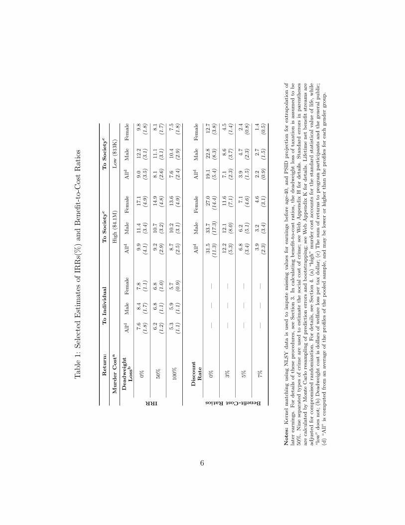
Table 1 summarizes the range of estimates from our preferred methodol-
ogy, defended later in this paper. Estimates from a diverse set of method-
ologies can be found in Web Appendix J. All point in the same direction.
Separate rates of return are reported for benefits accruing to individuals
versus those that accrue to society at large that include the impact of the
program on crime, participation in welfare, and the resulting savings in social
costs. Our estimate of the overall social rate of return to the Perry program
is in the range of 7–10 percent. We report a range of estimates because of
uncertainty about some components of benefits and costs for which standard
10See, e.g., MaCurdy (2007) for a survey of these methods.
5
Tab
le1:
Sel
ecte
dE
stim
ates
ofIR
Rs(
%)
and
Ben
efit-
to-C
ost
Rat
ios
Retu
rn
:T
oIn
div
idu
al
To
Socie
tyc
To
Socie
tyc
Mu
rd
er
Cost
aH
igh
($4.1
M)
Low
($13K
)
IRRD
ead
weig
ht
Loss
bA
lld
Male
Fem
ale
Alld
Male
Fem
ale
Alld
Male
Fem
ale
0%
7.6
8.4
7.8
9.9
11.4
17.1
9.0
12.2
9.8
(1.8
)(1
.7)
(1.1
)(4
.1)
(3.4
)(4
.9)
(3.5
)(3
.1)
(1.8
)
50%
6.2
6.8
6.8
9.2
10.7
14.9
8.1
11.1
8.1
(1.2
)(1
.1)
(1.0
)(2
.9)
(3.2
)(4
.8)
(2.6
)(3
.1)
(1.7
)
100%
5.3
5.9
5.7
8.7
10.2
13.6
7.6
10.4
7.5
(1.1
)(1
.1)
(0.9
)(2
.5)
(3.1
)(4
.9)
(2.4
)(2
.9)
(1.8
)
Benefit-CostRatios
Dis
cou
nt
Rate
Alld
Male
Fem
ale
Alld
Male
Fem
ale
0%
——
—31.5
33.7
27.0
19.1
22.8
12.7
(11.3
)(1
7.3
)(1
4.4
)(5
.4)
(8.3
)(3
.8)
3%
——
—12.2
12.1
11.6
7.1
8.6
4.5
(5.3
)(8
.0)
(7.1
)(2
.3)
(3.7
)(1
.4)
5%
——
—6.8
6.2
7.1
3.9
4.7
2.4
(3.4
)(5
.1)
(4.6
)(1
.5)
(2.3
)(0
.8)
7%
——
—3.9
3.2
4.6
2.2
2.7
1.4
(2.3
)(3
.4)
(3.1
)(0
.9)
(1.5
)(0
.5)
Note
s:K
ern
elm
atc
hin
gu
sin
gN
LS
Yd
ata
isu
sed
toim
pu
tem
issi
ng
valu
esfo
rea
rnin
gs
bef
ore
age-
40,
an
dP
SID
pro
ject
ion
for
extr
ap
ola
tion
of
late
rea
rnin
gs.
For
det
ails
of
thes
ep
roce
du
res,
see
Sec
tion
3.
Inca
lcu
lati
ng
ben
efit-
to-c
ost
rati
os,
the
dea
dw
eight
loss
of
taxati
on
isass
um
edto
be
50%
.N
ine
sep
ara
ted
typ
esof
crim
eare
use
dto
esti
mate
the
soci
al
cost
of
crim
e;se
eW
ebA
pp
end
ixH
for
det
ails.
Sta
nd
ard
erro
rsin
pare
nth
eses
are
calc
ula
ted
by
Monte
Carl
ore
sam
plin
gof
pre
dic
tion
erro
rsan
db
oots
trap
pin
g;
see
Web
Ap
pen
dix
Kfo
rd
etail
s.L
ifet
ime
net
ben
efit
stre
am
sare
ad
just
edfo
rco
mp
rom
ised
ran
dom
izati
on
.F
or
det
ails,
see
Sec
tion
4.
(a)
“h
igh
”m
urd
erco
stacc
ou
nts
for
the
stan
dard
stati
stic
al
valu
eof
life
,w
hil
e“lo
w”
does
not;
(b)
Dea
dw
eight
cost
isd
ollars
of
wel
fare
loss
per
tax
doll
ar;
(c)
Th
esu
mof
retu
rns
top
rogra
mp
art
icip
ants
an
dth
egen
eral
pu
blic;
(d)
“A
ll”
isco
mp
ute
dfr
om
an
aver
age
of
the
pro
file
sof
the
poole
dsa
mp
le,
an
dm
ay
be
low
eror
hig
her
than
the
pro
file
sfo
rea
chgen
der
gro
up
.
6

errors cannot be assigned. These estimates are above the historical return
to equity.11 However, our estimates are substantially below the estimates of
the rate of return to the Perry program reported in previous studies. This
difference is driven mainly by our approach to evaluating the social costs of
crime. We present an extensive sensitivity analysis of the consequences of
alternative assumptions about the social cost of crime for the estimated rate
of return. The benefit-to-cost ratios presented in the bottom of Table 1 sup-
port the rate of return analysis. The rest of the paper justifies the estimates
presented in Table 1.
This paper proceeds in the following way. Section 2 discusses the Perry
program and how it was evaluated. Section 3 discusses the sampling plan
used to collect the outcomes of the experiment and the empirical problems it
creates, which require imputation and extrapolation to compute the rate of
return. Problems of estimating non-market benefits of the program are also
discussed. Section 4 presents our estimates and their sensitivity to alternative
plausible assumptions. We contrast our approach with the approaches taken
by other analysts. In the final section, we summarize our findings and draw
conclusions.
11The estimated mean returns are above the post-World War II stock market rate ofreturn on equity of 5.8 percent (see DeLong and Magin, 2009).
7

2. Perry: Experimental Design and Background
The High/Scope Perry Preschool Program was an early childhood educa-
tion program conducted at the Perry Elementary School in Ypsilanti, Michi-
gan, during the early 1960s. Beginning at age three and lasting two years,
treatment consisted of a 2.5-hour preschool program on weekdays during the
school year, supplemented by weekly home visits by teachers.
The curriculum was based on supporting children’s cognitive and socio-
emotional development through active learning where both teachers and chil-
dren had major roles in shaping children’s learning. Children were encour-
aged to plan, carry out, and reflect on their own activities through a plan-do-
review process. Adults observed, supported, and extended children’s play as
appropriate. They also encouraged children to make choices, problem solve,
and engage in activities. Instead of providing lessons, Perry emphasized re-
flective and open-ended questions asked by teachers. Examples are: “What
happened? How did you make that? Can you show me? Can you help
another child?” (Schweinhart, Barnes, and Weikart, 1993, p. 33).12
Eligibility Criteria. Five cohorts of preschoolers were enrolled in the pro-
gram in the early to the mid-1960’s. Drawn from the community served
by the Perry Elementary School, participants were located through a sur-
vey of families associated with that school, as well as through neighborhood
12Web Appendix A provides further information on the program. See http://jenni.uchicago.edu/Perry/cba/.
8

group referrals, and door-to-door canvassing. Disadvantaged children living
in adverse circumstances were identified using IQ scores and a family socioe-
conomic status (SES) index. Those with IQ scores outside the range of 70-85
were excluded, as were those with untreatable mental defects.
The Compromised Randomization Protocol. A potential problem with the
Perry study is that after random assignment, treatment and controls were
reassigned, compromising the original random assignment and making sim-
ple interpretation of the evidence problematic. In addition, there was some
imbalance in the baseline variables between treatment and control groups.
Heckman, Moon, Pinto, Savelyev, and Yavitz (2009b) discuss the Perry selec-
tion and randomization protocols in detail. They correct for the imbalance in
preprogram variables and the compromise in randomization using matching.
We use their procedures in this analysis.13
13The randomization protocol used in the Perry Preschool Program was complex. Foreach designated eligible entry cohort, children were assigned to treatment and controlgroups in the following way. (1) Participant status of the younger siblings is the sameas that of their older siblings; (2) Those remaining were ranked by their entry IQ scorewith odd- and even-ranked subjects assigned to separate groups; (3) Some individualsinitially assigned to one group were swapped between groups to balance gender and meanSES scores, “with Standford-Binet scores held more or less constant”. This produced animbalance in family background variables; (4) A coin toss randomly selected one group asthe treatment group and the other as the control group; (5) Some individuals provisionallyassigned to treatment, whose mothers were employed at the time of the assignment, wereswapped with control individuals whose mothers were not employed. The rationale for thisswap was that it was difficult for working mothers to participate in home visits assignedto the treatment group. For further discussion of the Perry randomization protocol, seeAppendix L and Heckman, Moon, Pinto, Savelyev, and Yavitz (2009b).
9

Evidence on Selective Participation. Weikart et al. (1978) claim that “virtu-
ally all” eligible families agreed to participate in the program, implying that
there is no issue of bias arising from selective participation of more motivated
families from the pool of eligible participants.14
Study Follow-Up. Follow-up interviews were conducted when participants
were approximately 15, 19, 27, and 40 years old. Attrition remains low
throughout the study, with over 90 percent of the original sample partici-
pating in the age-40 interview. At these interviews, participants provided
detailed information about their lifecycle trajectories including schooling,
economic activity, marital life, child rearing, and incarceration. In addition,
Perry researchers collect administrative data in the form of school records,
police and court records, and welfare program participation records.
The Previous Literature and Its Critics. As the oldest and most cited early
childhood intervention evaluated by the method of random assignment, the
Perry study serves as a flagship for policy makers advocating public sup-
port for early childhood programs. Schweinhart et al. (2005) and Heckman,
Moon, Pinto, Savelyev, and Yavitz (2009b) find substantial treatment ef-
14Heckman, Moon, Pinto, Savelyev, and Yavitz (2009b) discuss the external validity ofthe Perry study. Using the NLSY sample of African Americans who were born in thesame years as the Perry participants, they estimate that 17% of the males and 15 % of thefemales in the NLSY would be eligible for the Perry program if it were applied nationwide.Perry over-represents the most disadvantaged segment of the African-American populationof children.
10

fects. Crime reduction is a major benefit of this program.15 The latter study
systematically addresses several important statistical issues that arise in ana-
lyzing the Perry data including its small sample size. The authors show that
for the Perry data small sample permutation inference (based on randomly
assigning treatment labels for treatments and controls) produces the same
inference about the null hypothesis of no treatment effect as is produced from
application of test statistics that are justified only in large samples. Thus,
concerns over the small sample size of the Perry study are unfounded.
Table 2 presents some descriptive statistics on treatment-control differ-
ences. Additional detail about the program can be found on the Web Ap-
pendix for this paper.
For the cost-benefit analysis of this program, the High/Scope Foundation
collaborated with outside researchers and produced cost-benefit analyses for
the age-27 and age-40 follow-up studies.16 An independent study was con-
ducted by Rolnick and Grunewald (2003). These studies report high internal
rates of return (IRR): 16 percent by Rolnick and Grunewald (2003) and 17
percent by Belfield et al. (2006). Our analysis challenges these estimates.
Unlike the estimates reported in previous studies, our estimated rates of re-
turn recognize problems with the data and problems raised by imbalances in
15Their findings are generally consistent with findings from a recent study of Head Start(Garces et al., 2002). Those authors find that African-Americans who participated inHead Start are significantly less likely to have been booked or charged with a crime.
16Barnett (1996) and Belfield, Nores, Barnett, and Schweinhart (2006), respectively.
11
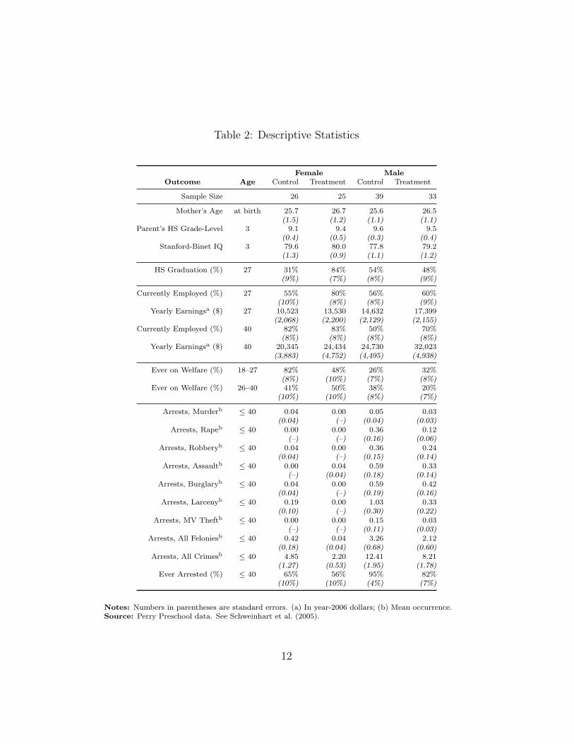
Table 2: Descriptive Statistics
Female MaleOutcome Age Control Treatment Control Treatment
Sample Size 26 25 39 33
Mother’s Age at birth 25.7 26.7 25.6 26.5(1.5) (1.2) (1.1) (1.1)
Parent’s HS Grade-Level 3 9.1 9.4 9.6 9.5(0.4) (0.5) (0.3) (0.4)
Stanford-Binet IQ 3 79.6 80.0 77.8 79.2(1.3) (0.9) (1.1) (1.2)
HS Graduation (%) 27 31% 84% 54% 48%(9%) (7%) (8%) (9%)
Currently Employed (%) 27 55% 80% 56% 60%(10%) (8%) (8%) (9%)
Yearly Earningsa ($) 27 10,523 13,530 14,632 17,399(2,068) (2,200) (2,129) (2,155)
Currently Employed (%) 40 82% 83% 50% 70%(8%) (8%) (8%) (8%)
Yearly Earningsa ($) 40 20,345 24,434 24,730 32,023(3,883) (4,752) (4,495) (4,938)
Ever on Welfare (%) 18–27 82% 48% 26% 32%(8%) (10%) (7%) (8%)
Ever on Welfare (%) 26–40 41% 50% 38% 20%(10%) (10%) (8%) (7%)
Arrests, Murderb ≤ 40 0.04 0.00 0.05 0.03(0.04) (–) (0.04) (0.03)
Arrests, Rapeb ≤ 40 0.00 0.00 0.36 0.12(–) (–) (0.16) (0.06)
Arrests, Robberyb ≤ 40 0.04 0.00 0.36 0.24(0.04) (–) (0.15) (0.14)
Arrests, Assaultb ≤ 40 0.00 0.04 0.59 0.33(–) (0.04) (0.18) (0.14)
Arrests, Burglaryb ≤ 40 0.04 0.00 0.59 0.42(0.04) (–) (0.19) (0.16)
Arrests, Larcenyb ≤ 40 0.19 0.00 1.03 0.33(0.10) (–) (0.30) (0.22)
Arrests, MV Theftb ≤ 40 0.00 0.00 0.15 0.03(–) (–) (0.11) (0.03)
Arrests, All Feloniesb ≤ 40 0.42 0.04 3.26 2.12(0.18) (0.04) (0.68) (0.60)
Arrests, All Crimesb ≤ 40 4.85 2.20 12.41 8.21(1.27) (0.53) (1.95) (1.78)
Ever Arrested (%) ≤ 40 65% 56% 95% 82%(10%) (10%) (4%) (7%)
Notes: Numbers in parentheses are standard errors. (a) In year-2006 dollars; (b) Mean occurrence.Source: Perry Preschool data. See Schweinhart et al. (2005).
12

preprogram variables between treatments and controls and by compromised
randomization. The previous studies are unable to answer many important
questions: How reliable are the IRR estimates? Can we conclude that the
estimated IRRs are statistically significantly different from zero? Are all as-
sumptions, accounting rules and estimation methods employed in previous
studies reasonable? How would different plausible earnings imputation and
extrapolation methods impact estimates of the IRR? If crime costs drive the
IRR results, as previous studies have found, what are the consequences of
estimating these costs under different plausible assumptions?
3. Program Costs and Benefits
The internal rate of return (IRR) is the annualized rate of return that
equates the present values of costs and benefits between treatment and con-
trol group members. Lifetime benefits and costs through age 40 are directly
measured using follow-up interviews. Extrapolation can be used to extend
these profiles through age 65. Alternatively, we also compute rates of return
through age 40 to eliminate uncertainty due to extrapolation. The scope of
our evaluation is confined to the costs and benefits of education, earnings,
criminal behavior, tax payments, and reliance on public welfare programs.
There are no reliable data on health outcomes, marital and parental out-
comes, the quality of social life and the like.17 Hence, our estimated rate of
17Appendix B summarizes the data sources which we use in this paper.
13

return likely understates the true rate of return, although we have no direct
evidence on this issue. We present separate estimates of rates of return for
private benefits and more inclusive social benefits.
3.1. Initial Program Cost
We use estimates of initial program costs reported in Barnett (1996).
These include both operating costs (teacher salaries and administrative costs)
and capital costs (classrooms and facilities). This information is summarized
in Web Appendix C. In undiscounted year-2006 dollars, cost of the program
per child is $17,759.
3.2. Program Benefits: Education
Perry promoted educational attainment through two avenues: total years
of education attained and rates of progression to a given level of educa-
tion. This pattern is particularly evident for females. Treated females re-
ceived less special education, progressed more quickly through grades, earned
higher GPAs, and attained higher levels of education than their control-
group counterparts. The statistical significance of these differences depends
on the methodology used, but all results point in the same direction. For
males, however, the impact of the program on schooling attainment is weak
at best.18
18This pattern was noted in Heckman (2005). Heckman, Moon, Pinto, Savelyev, andYavitz (2009b) discuss this phenomenon in the context of the local labor market in whichPerry participants reside. In the late 1970s, as Perry participants entered the workforce,the local male-friendly high-wage automotive manufacturing sector was booming. Persons
14

In this section, we report estimates of tuition and other pecuniary costs
paid by individuals to regular K-12 educational institutions, colleges, and
vocational training institutions, and additional social costs incurred by so-
ciety to educate them.19 The amount of educational expenditure that the
general public spends is greater if persons attain more schooling or if they
progress through school less efficiently. Web Appendix D presents detailed
information on educational attainment and costs in Perry.
K-12 Education. To calculate the cost of K-12 education, we assume that
all Perry subjects went to public school at the annual cost per pupil in the
state of Michigan during the period in question, $6,645.20 Treatment group
members spent only slightly more time in the K-12 system, in spite of the
discrepancy between treatment and control group graduation rates. Among
females, control subjects were held back in school more often. This equalized
the social cost of educating them in the K-12 system with the social cost
of the treatment group. Society spent comparable amounts of resources on
individuals during their K-12 education regardless of their treatment experi-
ence, albeit for different reasons. Most treatment females who stayed longer
did not need high school diplomas to get good entry-level jobs in manufacturing. (SeeGoldin and Katz, 2008.)
19All monetary values are in year-2006 dollars unless otherwise specified. Social costsinclude the additional funds beyond tuition paid required to educate students.
20See “Total expenditure per pupil in public elementary and secondary education” foryears 1974-1980, as reported by the Digest of Education Statistics (1975-1982, each year,in year-2006 dollars). We assume that public K-12 education entails no private cost forindividuals. Detailed per pupil expenditures for Ypsilanti schools are not available for therelevant years.
15

obtained diplomas, while most control females who stayed longer repeated
grades and many eventually dropped out of school. For males, educational
experiences were very similar between treatments and controls.
GED and Special Education. Some male dropouts acquired high school cer-
tificates through GED testing. Our estimates of the private costs of K-12
education include the cost of getting a GED.21 Female control subjects re-
ceived more special education than treatment subjects. For males, there was
no difference in receipt of special education by treatment status. Special
services require additional spending. To calculate this cost, we use estimates
from Chambers, Parrish, and Harr (2004), who provide a historical trend of
the ratio of per-pupil costs for special and regular education.22
2- and 4-Year Colleges. To calculate the cost of college education, we use
each individual’s record of credit hours attempted multiplied by the cost per
credit hour (including both student-paid tuition costs and public institutional
expenditures), taking into account the type of college attended.23 Male con-
21For detailed statistics about the GED, see Heckman and LaFontaine (2008).22In 1968–69, this ratio was about 1.92; in 1977–78, it was 2.17. Since Perry subjects
attended K-12 education in the interval between these two periods, we set the ratio to 2and apply it to all K-12 schooling years, which gives an additional $6,645 annual per-pupilcost for special education.
23Total cost is the sum of private tuition and public expenditure. For student-paidtuition costs at a 2-year college, we use the 1985 tuition per credit hour for WashtenawCommunity College ($29); for a 4-year college, that of Michigan State University for thesame year ($42). To calculate public institutional expenditure per credit hour, we dividethe national mean of total per-student annual expenditure (National Center for EducationStatistics, 1991, “Expenditure per Full-Time-Equivalent Student”, Table 298) by 30, atypical credit-hour requirement for full-time students at U.S. colleges. This calculationyields $590 per credit hour for 2-year colleges and $1,765 for 4-year colleges.
16

trol subjects attended more college classes than male treatment subjects —
the reverse of the pattern for females. As a result, the social cost of college
education is bigger for the control group among males while it is bigger for
the treatment group among females.
After the age-27 interview, many Perry subjects progressed to higher ed-
ucation. Without having detailed information about educational attainment
between the age-27 and age-40 interviews, we make some crude cost esti-
mates. For college education, we assume “some college education” to be
equivalent to 1-year attendance at a 2-year college. For 2-year or 4-year col-
lege degrees, we take the tuition and expenditure estimates used for college
going before age 27.24 Without detailed information on whether a subject
did or did not get any financial support, we assume that the private cost for
a 2-year master’s degree is the same as that for a 4-year bachelor’s degree.
Control males and treatment females pursued higher education more vig-
orously than did their same-sex counterparts, although only the treatment
effect for females is statistically significant.
Vocational Training. Some subjects attended vocational training programs.
Among males, control group members were more likely to attend vocational
programs, although the treatment effect is not precisely determined. Among
females, the pattern is reversed and the treatment effect is precisely deter-
mined. Thus, the public spent more resources to train control males and
24For missing information on educational attainment, we use the corresponding gender-treatment group mean.
17

treatment females than their respective counterparts.25 Individual costs are
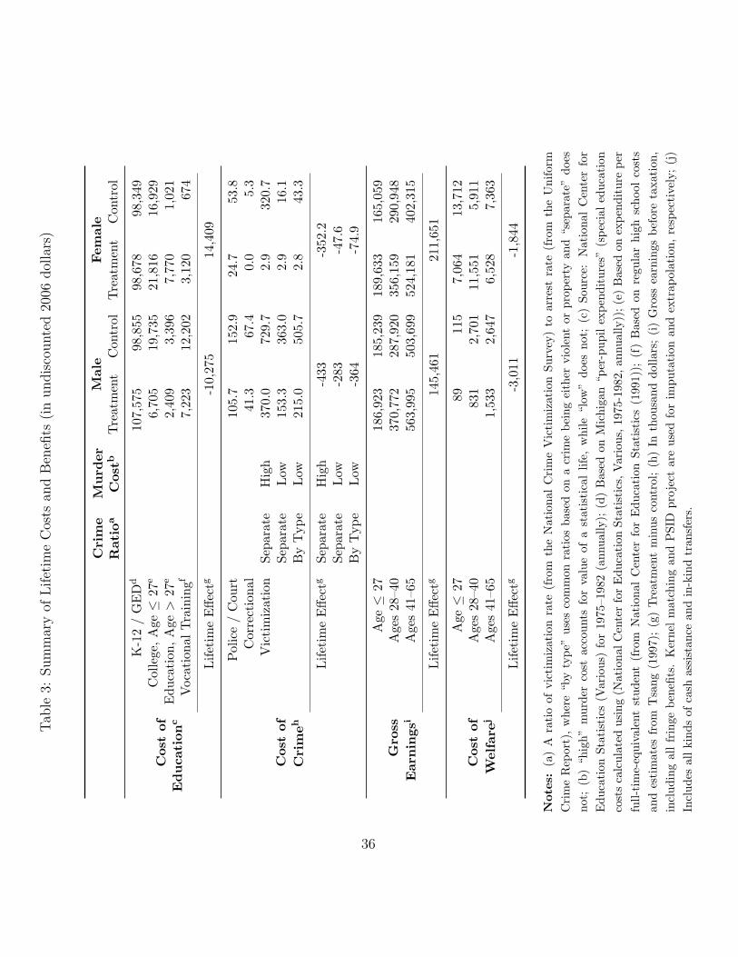
calculated using the number of months each Perry subject attended a voca-
tional training institute. Table 3 summarizes the components of estimated
educational costs. The other components of costs and benefits are discussed
later.
3.3. Program Benefits: Employment and Earnings
To construct lifetime earnings profiles, we must solve two practical prob-
lems. First, job histories were constructed retrospectively only for a fixed
number of previous job spells.26 Missing data must be imputed using econo-
metric techniques. Second, data on the Perry sample ends at the time of
the age-40 interview. In order to generate lifetime profiles, it is necessary to
predict earnings profiles beyond this age or else to estimate rates of return
through age 40. The latter assumption is conservative in assuming no per-
sistence of treatment effects past age 40. We report both sets of estimates
in this paper. The proportion of non-missing earnings data is about only 70
25We assume that all costs are paid by the general public. Estimates by Tsang (1997)suggest per-trainee costs which are 1.8 times the per-pupil costs of regular high schooleducation.
26At each interview, participants were asked to provide information about their em-ployment history and earnings at each job for several previous jobs. From this interviewdesign, three problems arise. First, for people with high job mobility, some past jobs areunreported. Second, for people who were interviewed in the middle of a job spell, it maynot be possible to precisely specify the end point of that job spell — that is, we have a“right-censoring” problem for the job spells at the time of interview. Third, even when thedates for each job spell can be precisely specified, it is not possible to identify how earningprofiles evolve within each job spell because an interviewee reports only one earnings valuefor each job.
18

percent for ages 19–40. Web Appendix G presents descriptive statistics and
the procedures used to extrapolate earnings when extrapolation is used.
Imputation. To impute missing values for periods prior to the age-40 inter-
view, we use four different imputation procedures and compare the estimates
based on them. First, we use simple piecewise linear interpolation, based on
weighted averages of the nearest observed data points around a missing value.
This approach is used by Belfield, Nores, Barnett, and Schweinhart (2006).
For truncated spells,27 we first impute missing employment status with the
mean of the corresponding gender-treatment data from the available sample
at the relevant time period, and then we interpolate. Second, we impute miss-
ing values using estimated earnings functions fit on a matched 1979 National
Longitudinal Survey of Youth (NLSY79) “low-ability”28 African-American
subsample of the same age as Perry subjects. Heckman, Moon, Pinto, Save-
lyev, and Yavitz (2009b) show that this subsample from the NLSY79 is sim-
ilar in characteristics and outcomes to the Perry controls. The NLSY79
longitudinal data are far more complete than the Perry data. We estimate
earnings functions for each NLSY79 gender-age cross-section using education
27As noted in the previous footnote, there are job spells in progress at the time ofinterview.
28This “low-ability” subsample is selected by initial background characteristics thatmimic the eligibility rule actually used in the Perry program. NLSY79 is a nationally-representative longitudinal survey whose respondents are almost at the same age (birthyears 1956–1964) as the Perry sample (birth years 1957–1962). We extract a comparisongroup from this data using birth order, socioeconomic status (SES) index, and AFQT testscore. These restrictions are chosen to mimic the program eligibility criteria of the Perrystudy. For details, see Web Appendix F.
19
dummies, work experience and its square as regressors and then impute from
this equation the missing values for the corresponding Perry gender-age cross-
section. For truncated spells, we assume symmetry around the truncation
points. Third, we use a kernel procedure that matches each Perry subject
to similar observations in the NLSY79 sample to impute missing values in
Perry. Each Perry subject is matched to all observations in the NLSY79 com-
parison group sample, but with different weights that depend on a measure
of distance in characteristics between Perry experimentals, and comparison
group members.29 This procedure weights more heavily NLSY sample par-
ticipants who more closely match Perry subjects. For truncated spells, we
first match the length of spells, and then earnings. Fourth, we estimate dy-
namic earnings functions using the method of Hause (1980), discussed by
MaCurdy (2007), for each NLSY79 age-gender group. This procedure de-
composes individual earnings processes into observed abilities, unobserved
time-invariant components and serially correlated shocks. The procedure
uses the estimated parameters of the Hause model to impute missing val-
ues in the Perry earnings data. For truncated spells, we assume symmetry
around truncation points. All four methods are conservative in that they
impose the same earnings structure on the missing data for treatment and
controls. The fourth method preserves differences in pre-existing patterns of
unobservables between treatments and controls. See Appendix G for further
29We use the Mahalanobis (1936) distance.
20

discussion.
Extrapolation. Given the absence of earnings data after age 40, we employ
three extrapolation schemes to extend sample earnings profiles to later ages.
First, we use March 2002 Current Population Survey (CPS) data to obtain
earnings growth rates up to age 65. Since the CPS does not contain measures
of cognitive ability, it is not possible to extract “low ability” subsamples
from the CPS that are comparable to the Perry control group. We use
CPS age-by-age growth rates (rather than levels of earnings) of three-year
moving average of earnings by race, gender, and educational attainment to
extrapolate earnings, thereby avoiding systematic selection effects in levels.30
We link the CPS changes to the final Perry earnings. Second, we use the
Panel Study of Income Dynamics (PSID) to extrapolate earnings profiles
past age-40. In the PSID, there is a word-completion test score from which
we can extract a “low ability” subsample in a fashion similar to the way
we extract a matched sample from the NLSY79 using AFQT scores.31 To
extrapolate Perry earnings profiles, we first estimate a random effects model
of earnings using lagged earnings, education dummies, age dummies and
a constant as regressors. We use the fitted model to extrapolate earnings
30Belfield et al. (2006) use mean values of CPS earnings in their Perry extrapolations.In doing so, they neglect the point that Perry subjects belong to the bottom of the distri-bution of ability and the further point that CPS subjects are sampled from a more generalpopulation with higher average ability.
31For information on how we extract this subsample from PSID, see Web Appendix F.
21

after age 40.32 Third, we also use individual parameters from an estimated
Hause (1980) model. For computing rates of return, we obtain complete
lifetime earnings profiles from these procedures and compare the results of
using alternative approaches to extrapolation on estimated rates of return.33
All three methods are conservative in that they impose the same earnings
dynamics on treatments and controls. However, in making projections all
three methods account for age-40 individual earnings differences between
treatments and controls.
The earnings analyzed in Table 3 and Web Appendix G (Tables G.4 and
G.5), include all types of fringe benefits listed in Employer Costs for Em-
ployee Compensation (ECEC), a Bureau of Labor Statistics (BLS) compen-
sation measure. Even though the share of fringe benefits in total employee
compensation varies across industries, due to data limitations, our calcula-
tions assume the share to be constant at its economy-wide average regardless
of industry.34
32By taking residuals from a regression of earnings on a constant, period dummies andbirth year dummies, we can remove fluctuations in earnings due to period-specific andcohort-specific shocks. See Rodgers et al. (1996) for a description of the procedure we use.
33For all profiles used here, survival rates by age, gender and education also are incor-porated, which are obtained from National Vital Statistics Reports (2004). Belfield et al.(2006) do not account for negative correlation between educational attainment and deathrates.
34The share of fringe benefit has fluctuated over time with the historical average ofabout 30 percent. Given the limitations of our data, we apply the economy-wide averageshare at the corresponding year to each person’s earnings assuming all fringe benefits aretax-free.
22
3.4. Program Benefits: Criminal Activity
Crime reduction is a major benefit of the Perry program.35 Valuing the
effect of crime reduction in terms of costs and benefits is not trivial given the
difficulty in assigning reliable monetary values to non-market outcomes. In
this sub-section, we improve on the previous studies (for example, Belfield
et al. (2006)) by exploring the impact on rates of return and cost-benefit
analysis of a variety of assumptions and accounting rules. For each subject,
the Perry data provide a full record of arrests, convictions, charges and in-
carcerations for most of the adolescent and adult years. They are obtained
from administrative data sources.36 The empirical challenges addressed in
this section are twofold: obtaining a complete lifetime profile of criminal ac-
tivities for each person, and assigning values to that criminal activity. Web
Appendix H presents a comprehensive analysis of the crime data which we
summarize in this section.
35See, for example, Schweinhart et al. (2005), and Heckman, Moon, Pinto, Savelyev,and Yavitz (2009b). Table 2 shows that the effect is mainly due to males. Heckman, Mal-ofeeva, Pinto, and Savelyev (2009a) find evidence that may explain this pattern. Programtreatment effects for males mainly operate through enhancing noncognitive or behavioralskills that are very predictive of criminal behavior.
36The earliest records cover ages 8–39 and the oldest cover ages 13–44. However, thereare some limitations. At the county (Washtenaw) level, arrests, all convictions, incarcer-ation, case numbers, and status are reported. At the state (Michigan) level, arrests areonly reported if they lead to convictions. For the 38 Perry subjects spread across the 19states other than Michigan at the time of the age-40 interview, only 11 states providedcriminal records. No corresponding data are provided for subjects residing abroad.
23

3.4.1. Lifetime Crime Profiles
Even though the arrest records for Perry participants cover most of their
adolescent and adult lives, information about criminal activities stops at the
time of the age-40 interview. To overcome this problem, we use national
crime statistics published in the Uniform Crime Report (UCR), which are
collected by the Federal Bureau of Investigation (FBI) from state and local
agencies nationwide. The UCR provides arrest rates by gender, race, and
age for each year. We apply population rates to estimate missing crime.37
See the discussion in Web Appendix H.
3.4.2. Crime Incidence
Estimating the impact of the program on crime requires estimating the
true level of criminal activity at each age and obtaining reasonable estimates
of the social cost of each crime. For a crime of type c at time t, the total
social cost of that crime V ct can be calculated as a product of the social cost
per unit of crime Cct and the incidence Ic
t :
V ct = Cc
t × Ict .
We do not directly observe the true incidence level Ict . Instead, we only
observe each subject’s arrest record at age t for crime c, Act .
38 If we know
37We use the year-2002 UCR for this extrapolation.38Given these data limitations, we do not model each individual’s criminal behavior so
that we are not able to fully account for the individual level dynamics of criminality. Weaddress the heterogeneity of criminal activity across Perry sample members by including
24

the incidence-to-arrest ratio Ict /A
ct from other data sources, we can estimate
V ct by multiplying the three terms in the following expression:
V ct = Cc
t ×Ict
Act
× Act .
To obtain the incidence-to-arrest ratio Ict /A
ct for each crime of type c at
time t, we use two national crime datasets: the Uniform Crime Report (UCR)
and the National Crime Victimization Survey (NCVS).39 The UCR provides
comprehensive annual arrest data between 1977 and 2004 for state and local
agencies across the U.S. The NCVS is a nationally-representative household-
level data set on criminal victimization which provides information on levels
of unreported crime across the U.S. By combining these two sources, we can
calculate the incidence-to-arrest ratio for each crime of type c at time t.
As noted in the UCR (2002), however, the crime typologies derived from the
UCR and those of the NCVS are “not strictly comparable.” To overcome this
problem, we developed a unified categorization of crimes across the NCVS,
UCR, and Perry data sets for felonies (Web Appendix H, Table H.4) and
misdemeanors (Web Appendix H, Table H.5). Web Appendix H, Table H.7,
shows our estimated incidence-to-arrest ratios for these crimes. To check the
a number of tables and figures in the Web Appendix H on estimation of the costs of crimeand by conducting sensitivity analyses at the aggregate level by including or excluding agroup of “hardcore” criminals who repeat crimes.
39The Federal Bureau of Investigation website provides annual reports based on UCR(http://www.fbi.gov/ucr/ucr.htm). NCVS are available at Department of Justice web-site (http://www.ojp.usdoj.gov/bjs/cvict.htm).
25

sensitivity of our results to the choice of a particular crime categorization,
we use two sets of incidence-to-arrest ratios and compare results. For the
first set, we assume that each crime type has a different incidence-to-arrest
ratio. These are denoted “Separated” in our tables. For the second set, we
use two broad categories, violent vs. property crime. These are denoted by
“Property vs. Violent” in our tables. Further, to account for local context,
we calculate ratios using UCR/NCVS crime levels that are geographically
specific to the Perry program: only crimes committed or arrests made in
Metropolitan Sampling Areas of the Midwest.40
3.4.3. Unit Costs of Crime
Using a simplified version of a decomposition developed in Anderson
(1999) and Cohen (2005), we divide crime costs into victim costs and Crim-
inal Justice System costs, which consist of police, court, and correctional
costs.
Victim Costs. To obtain total costs from victimization levels, we use unit
costs from Cohen (2005). Different types of crime are associated with dif-
ferent victimization unit costs. Some crimes are not associated with any
victimization costs. In Web Appendix H, Table H.13, we summarize the unit
cost estimates used for different types of crime.
40For this purpose, the Midwest is defined as Ohio, Michigan, Indiana, Illinois, Wis-consin, Minnesota, Iowa, Missouri, North Dakota, South Dakota, Nebraska, and Kansas.The City of Ypsilanti, where the Perry program was conducted, belongs to the DetroitMetropolitan Sampling Area. For a comparison of these ratios between the local andnational levels, see Web Appendix H.3.
26

Police and Court Costs. Police, court, and other administrative costs are
based on Michigan-specific cost estimates per arrest calculated from the UCR
and Expenditure and Employment Data for the Criminal Justice System
(CJEE) micro datasets.41 Since we only observe arrests, and do not know
whether and to what extent the courts were involved (for example, whether
there was a trial ending in acquittal), we assume that each arrest incurred
an average level of all possible police and court costs. This unit cost was
applied to all observed arrests (regardless of crime type).
Correctional Costs. Estimating correctional costs in Perry is a more straight-
forward task, as the data include a full record of incarceration and pa-
role/probation for each subject. To estimate the unit cost of incarceration,
we use expenditures on correctional institutions by state and local govern-
ments in Michigan divided by the total institution population. To estimate
the unit cost of parole/probation, we perform a similar calculation.42
41From Bureau of Justice Statistics (2003), we obtain total expenditures on police andjudicial-legal activities by federal, state, and local governments. We divide the expendi-tures from Michigan state and local governments by the total arrests in this area obtainedfrom UCR. To account for federal agencies’ involvement, we add another per-arrest po-lice/court cost which is calculated by dividing the total expenditure of federal governmentwith the total arrests at national level. This calculation is done for years 1982, 1987, 1992,1997, and 2002. For periods between selected years, we use interpolated values. See WebAppendix H.
42Belfield et al. (2006) compute crime-specific criminal-justice system costs. Eventhough in principle this approach could be more accurate than ours, we do not adoptit in this paper because their data source is questionable and we could not find any otherrelevant sources. Their unit cost estimates are obtained from a study of the police andcourts of Dade County, Florida which has quite different characteristics from WashtenawCounty, Michigan where the Perry experiment was conducted. We examine the sensitivityof our estimates to alternate ways to measure costs in Table 5. See Web Appendix H for
27

3.4.4. Estimated Social Costs of Crime
Table 3 summarizes our estimated social costs of crime. Our approach
differs from that used by Belfield et al. (2006) in several respects. First,
in estimating victimization-to-arrest ratios, police and court costs, and cor-
rectional costs, we use local data rather than national figures. Second, we
use two different values of the victim cost of murder: an estimate of “the
statistical value of life” ($4.1 million) and an estimate of assault victim cost
($13,000).43 We report separate rates of return for each estimate. Only four
murders are observed in the Perry arrest records.44 If one uses the statisti-
cal value of life as the cost of murder to the victim, a single murder might
dominate the calculation of the rate of return. To avoid this problem, Bar-
nett (1996) and Belfield et al. (2006) assign murder the same low cost as
assault. We adopt this method as one approach for valuing the social cost
of murder, but we also explore an alternative that includes the statistical
value of life in murder victimization costs. Contrary to intuition, however,
assuming a lower murder cost is not “conservative” in terms of estimating the
rate of return because the lone treated male murderer committed his crime
at a very early age (21) while the two control male murderers committed
their crimes in their late 30s. As a result, assigning a high victimization cost
further discussion.43See Cohen (2005) and, for a literature review, see Viscusi and Aldy (2003), who
provides a range of $2-9 million for the value of a statistical life.44One is committed by a control female, two by control males, and one by a treated
male.
28

to murder decreases the rate of return for males. Given the temporal pat-
tern of murder, we present rate-of-return estimates using both “high” and
“low” victim costs for murder (the former includes the statistical value of
life, and the latter does not) and compare the results. Third, we assume
that there are no victim costs associated with “driving misdemeanors” and
“drug-related crimes”. Whereas previous studies have assigned non-trivial
victim costs to these types of crimes, we consider them to be “victimless”.
Although such crimes could be the proximal cause of victimizations, such
victimizations would be directly associated with other crimes for which we
already account.45 This approach results in a substantial decrease of crime
cost compared to the cost of crime used in previous studies because these
specific crimes account for more than 30 percent of all crime reported in the
Perry study.
3.5. Tax Payments
Taxes are transfers from the taxpayer to the rest of society, and represent
benefits to recipients that reduce the welfare of the taxed unless services are
received in return. Our analysis considers benefits to recipients, benefits to
45“Driving misdemeanors” include driving without a license; suspended license; driv-ing under the influence of alcohol or drugs; other driving misdemeanors; failure to stopat an accident; improper license plate. “Drug-related crimes” include drug abuse, sale,possession, or trafficking. Belfield et al. (2006) use $3,538 to evaluate the cost of “drivingmisdemeanors” and $2,620 for “drug-related crimes” (in year-2006 dollars). Rolnick andGrunewald (2003) do not document how they treat crime. Belfield et al. (2006) computeexpected victim costs for these cases, which include, for example, probable risk of death.This practice leads to double counting, and thus to overstating savings in victimizationcosts due to the Perry program.
29

the public, and total social benefits (or costs). The latter category nets out
transfers but counts costs of collecting and avoiding taxes.
Higher earnings translate into higher absolute amounts of income tax
payments (and consumption tax payments) that are beneficial to the general
public excluding program participants. Since U.S. individual income tax
rates and the corresponding brackets have changed over time, in principle we
should apply relevant tax rates according to period, income bracket, and filing
status. In addition, most wage earners must pay the employee’s share of the
Federal Insurance Contribution Act (FICA) tax, such as the Social Security
tax and the Medicare tax. In 1978, the employee’s marginal and average
FICA tax rate for a four-person family at a half of US median income was
6.05 percent of taxable earnings. It gradually increased over time, reaching
7.65 percent in 1990, and has remained at that level ever since.46 Here, we
simplify the calculation by applying a 15 percent individual tax rate and
7.5 percent FICA tax rate to each subject’s taxable earnings in each year.47
Belfield, Nores, Barnett, and Schweinhart (2006) use the employer’s share of
FICA tax in addition to these two components in computing the benefit to
the general public, but we do not. A recent consensus among economists is
that “employer’s share of payroll taxes is passed on to employees in the form
46See Tax Policy Center (2007).47The “effective” tax rate for the working poor is much higher than this because people
lose eligibility for various welfare programs or withdraw benefits as income increases. SeeMoffitt (2003). Because, in computing the rate of return, we account for the effects ofPerry on all kinds of welfare benefits, including in-kind transfers, we apply the baselinetax rates to earnings data alone to avoid double-counting.
30

of lower wages than would otherwise be paid.”48 Since this tax burden is
already incorporated in realized earnings, we do not count it in computing
the benefit accrued to the general public while employers who are also among
the general public pay some money to the government. Web Appendix J,
Tables J.1–J.3, show how individual gross earnings are decomposed into net
earnings and tax payments under this assumption.
3.6. Use of the Welfare System
Most Perry subjects were significantly disadvantaged and received consid-
erable amounts of financial and non-financial assistance from various welfare
programs. Differentials in the use of welfare are another important source of
benefit from the Perry program. We distinguish transfers, which may benefit
one group in the society at the expense of another, from the costs associated
with making such transfers. Only the latter should be counted in computing
gains to society as a whole.
We have two types of information on the use of the welfare system: inci-
dence of welfare dependence, and actual welfare payments. Web Appendix I,
Table I.1, presents descriptive statistics comparing welfare incidence, the
length of welfare spells, and the welfare benefits that are actually received
by treatments and controls. One finding is that control females depend on
welfare programs more heavily than treatment females before age 27. That
48Congressional Budget Office (2007). Anderson and Meyer (2000) present empiricalevidence supporting this view.
31

pattern is reversed at later ages.49 For males, the scale of welfare usage is
lower, with controls more likely to use welfare at all ages.
Two types of data limitations affect our calculation. One is that we do not
have enough information about receipt of various in-kind transfer programs,
such as medical, housing, education, and energy assistance, which represent
a large portion of total U.S. welfare expenditures. The other is that even for
cash assistance programs such as General Assistance (GA), AFDC/TANF,
and Unemployment Insurance (UI), we do not have complete lifetime profiles
of cash transfers for each individual. Given these limitations, we adopt the
following method to estimate full lifetime profiles of welfare receipt.
First, we use the NLSY79 and PSID comparison samples to impute the
amount received from various cash assistance and food stamp programs.
Prior to age 27, we employ the NLSY79 black “low ability” subsample. Since
only the total number of months on welfare programs is known for the Perry
sample during this age range, such imputations are unavoidable. We im-
49Belfield et al. (2006) suggest that “delayed child-rearing and higher educational at-tainment” among treatment females can explain this phenomenon. However, this patternis at odds with evidence from the NLSY79 in which greater use of welfare is associatedwith lower educational attainment. Bertrand, Luttmer, and Mullainathan (2000) showthat a person’s welfare participation can be affected by behaviors of others in a network.Since the Perry program was conducted in a small town (Ypsilanti, Michigan) and thetreated females have known each other from their childhood, they could presumably shareand exchange information about welfare programs. This may have made it easier forthem to apply and receive benefits. In the NLSY79 which samples randomly from manycommunities, this effect is unlikely to be at work. If the network effect dominated, theobserved contradictory pattern should be interpreted as the composite of treatment effectand network effect. While having a better social network also could be a treatment effect,this distinction would be useful for investigating the external validity of this program.
32

pute individual monthly welfare receipt for each year using coefficients from
NLSY79 individual welfare payments for the corresponding year regressed on
gender and education indicators, a dummy variable for teenage pregnancy,
number of months in wedlock, employment status, earnings, and the number
of biological children.50 In this regression, welfare payments include food
stamps and all kinds of cash assistance available in the NLSY79 dataset,
such as Unemployment Insurance (UI), AFDC/TANF, Social Security, Sup-
plemental Security Income (SSI), and any other cash assistance. For ages
28–40, the Perry records provide both the total number of months on wel-
fare and the cumulative amount of receipts through UI, AFDC, and food
stamps. We use the observed amounts for these programs. For other welfare
programs, we use a regression-based imputation scheme similar to that used
to analyze the data prior to age 27. The total amount is computed as a
sum of these two components. To extrapolate this profile past age 40, we
use the PSID dataset, which contains profiles over longer stretches of the
life cycle than does the NLSY79. As with the earnings extrapolation, we
target the “low-ability” subsample of the PSID dataset. We first estimate a
random effects model of welfare receipt using a lagged dependent variable,
education dummies, age dummies, and a constant as regressors. We use the
fitted model to extrapolate. As with the NLSY79 imputation, the dependent
variable in this model includes all cash assistance and food stamps.51
50The exact imputation equation is given in Web Appendix I.51We remove cohort and year effects. See Web Appendices G and I.
33

Second, to account for in-kind transfers, we employ the Survey of Income
and Program Participation (SIPP) data. In SIPP, we calculate the probabil-
ity of being in specific in-kind transfer programs for a “less-educated” black
population born between the years 1956 and 1965, using the year-1984, -
1996, and -2004 micro datasets.52 We estimate linear probability models for
participation in each of a variety of programs using gender and educational
attainment variables as predictors.53 This calculation is done separately for
Medicaid, Medicare, housing assistance, education assistance, energy assis-
tance, public training programs, and other public service programs. We
interpolate values for missing data in periods between the years of available
data for each SIPP series. Past 2004, we use year-2004 estimates assuming
that the current welfare system continues. To convert this probability to
monetary values, we use estimates of Moffitt (2003) for real expenditures
on the combined federal, state, and local spending for the largest 84 means-
tested transfer programs. We adjust upward cash assistance amounts by a
product of the probability of participation in each program and the ratio of
real expenditures of the in-kind program to that of cash assistance, so that
the resulting amount becomes the expected cash value of in-kind receipt. We
aggregate across programs to obtain overall totals. Table 3 summarizes our
estimated profiles of welfare use.
52Since SIPP does not contain any kind of ability measure, we use a subsample whoseeducational attainment is less than or equal to “some college credits without diploma.”
53We fit the same equation to both treatment and control group members.
34

For society, each dollar of welfare involves administrative costs. Based
on Michigan state data, Belfield, Nores, Barnett, and Schweinhart (2006)
estimate a cost to society of 38 cents for every dollar of welfare disbursed.
We use this estimate to calculate the cost of welfare programs to society.54
3.7. Other Program Benefits
Other possibly beneficial effects of the Perry program that are not easily
quantified include the psychic cost of education, the utility gain from commit-
ting crime, the value of leisure, the value of marital and parental outcomes,
the contribution of the program to child care, the value of wealth accumu-
lation, the value of social life, the value of improved health and longevity,
and any intergenerational effects of the program.55 These benefits are not
included in our analysis due to data limitations.
4. Internal Rates of Return and Benefit-To-Cost Ratios
In this section, we calculate internal rates of return and benefit-to-cost
ratios for the Perry program under various assumptions and estimation meth-
ods. The internal rate of return (IRR) compares alternative investment
54This cost consists of two components: the cost of administering welfare disbursementand the cost accrued due to overpayments and payments to ineligible families.
55In this study, we do not include the child care cost that parents of program subjectswould have paid without this program. Thus, we likely underestimate the true benefits.Belfield, Nores, Barnett, and Schweinhart (2006) count child care for participants as abenefit, even for women who do not work, and hence they inflate the benefits of the Perryprogram. The effect of the program on longevity is accounted for to some degree becausewe adjust all profiles used in this study for survival rates by age, gender and educationalattainments.
35
Tab
le3:
Sum
mar
yof
Lif
etim
eC
osts
and
Ben
efits
(in
undis
counte
d20
06dol
lars
)
Cri
me
Rat
ioa
Murd
erC
ostb
Mal
eFem
ale
Tre
atm
ent
Con
trol
Tre
atm
ent
Con
trol
Cos
tof
Educa
tion
c
K-1
2/
GE
Dd
107,
575
98,8
5598
,678
98,3
49C
olle
ge,
Age≤
27e
6,70
519
,735
21,8
1616
,929
Edu
cati
on,
Age>
27e
2,40
93,
396
7,77
01,
021
Voc
atio
nal
Tra
inin
gf7,
223
12,2
023,
120
674
Life
tim
eE
ffect
g-1
0,27
514
,409
Cos
tof
Cri
meh
Pol
ice
/C
ourt
105.
715
2.9
24.7
53.8
Cor
rect
iona
l41
.367
.40.
05.
3V
icti
miz
atio
nSe
para
teH
igh
370.
072
9.7
2.9
320.
7Se
para
teL
ow15
3.3
363.
02.
916
.1B
yT
ype
Low
215.
050
5.7
2.8
43.3
Life
tim
eE
ffect
gSe
para
teH
igh
-433
-352
.2Se
para
teL
ow-2
83-4
7.6
By
Typ
eL
ow-3
64-7
4.9
Gro
ssEar
nin
gsi
Age≤
2718
6,92
318
5,23
918
9,63
316
5,05
9A
ges
28–4
037
0,77
228
7,92
035
6,15
929
0,94
8A
ges
41–6
556
3,99
550
3,69
952
4,18
140
2,31
5
Life
tim
eE
ffect
g14
5,46
121
1,65
1
Cos
tof
Wel
fare
j
Age≤
2789
115
7,06
413
,712
Age
s28
–40
831
2,70
111
,551
5,91
1A
ges
41–6
51,
533
2,64
76,
528
7,36
3
Life
tim
eE
ffect
g-3
,011
-1,8
44
Not
es:
(a)
Ara
tio
ofvi
ctim
izat
ion
rate
(fro
mth
eN
atio
nal
Cri
me
Vic
tim
izat
ion
Surv
ey)
toar
rest
rate
(fro
mth
eU
nifo
rmC
rim
eR
epor
t),
whe
re“b
yty
pe”
uses
com
mon
rati
osba
sed
ona
crim
ebe
ing
eith
ervi
olen
tor
prop
erty
and
“sep
arat
e”do
esno
t;(b
)“h
igh”
mur
der
cost
acco
unts
for
valu
eof
ast
atis
tica
llif
e,w
hile
“low
”do
esno
t;(c
)So
urce
:N
atio
nal
Cen
ter
for
Edu
cati
onSt
atis
tics
(Var
ious
)fo
r19
75–1
982
(ann
ually
);(d
)B
ased
onM
ichi
gan
“per
-pup
ilex
pend
itur
es”
(spe
cial
educ
atio
nco
sts
calc
ulat
edus
ing
(Nat
iona
lCen
ter
for
Edu
cati
onSt
atis
tics
,Var
ious
,197
5-19
82,a
nnua
lly))
;(e)
Bas
edon
expe
ndit
ure
per
full-
tim
e-eq
uiva
lent
stud
ent
(fro
mN
atio
nal
Cen
ter
for
Edu
cati
onSt
atis
tics
(199
1));
(f)
Bas
edon
regu
lar
high
scho
olco
sts
and
esti
mat
esfr
omT
sang
(199
7);
(g)
Tre
atm
ent
min
usco
ntro
l;(h
)In
thou
sand
dolla
rs;
(i)
Gro
ssea
rnin
gsbe
fore
taxa
tion
,in
clud
ing
all
frin
gebe
nefit
s.K
erne
lm
atch
ing
and
PSI
Dpr
ojec
tar
eus
edfo
rim
puta
tion
and
extr
apol
atio
n,re
spec
tive
ly;
(j)
Incl
udes
all
kind
sof
cash
assi
stan
cean
din
-kin
dtr
ansf
ers.
36

projects in a common metric. For each gender and treatment group, we
construct average life cycle benefit and cost profiles and then compute IRRs.
We also compute standard errors for all of the estimated IRRs and benefit-to-
cost ratios. The computation of standard errors is constructed in three steps.
In the first step, we use the bootstrap to simultaneously draw samples from
Perry, the NLSY79, and the PSID.56 For each replication, we re-estimate
all parameters that are used to impute missing values, and re-compute all
components used in the construction of lifetime profiles. Notice that in this
process, all components whose computations do not depend on the compar-
ison group data also are re-computed (e.g., social cost of crime, educational
expenditure, etc.) because the replicated sample consists of randomly drawn
Perry participants. In the second step, we adjust all imputed values for
prediction errors on the bootstrapped sample by plugging in an error term
which is randomly drawn from comparison group data by a Monte Carlo
resampling procedure. Combining these two steps allows us to account for
both estimation errors and prediction errors. Finally we compute point esti-
mates of IRRs for each replication to obtain bootstrap standard errors. Web
Appendix K describes in greater detail the procedure used to compute our
standard errors.
Table 4 and Web Appendix J show estimated IRR’s computed using var-
ious methods for estimating earnings profiles and crime costs and under var-
56For procedures that use different nonexperimental samples, we conduct the same ana-lyis.
37

Tab
le4:
Inte
rnal
Rat
esof
Ret
urn
(%),
by
Imputa
tion
and
Extr
apol
atio
nM
ethod
and
Ass
um
pti
ons
Ab
out
Cri
me
Cos
tsA
ssum
ing
50%
Dea
dw
eigh
tC
ost
ofT
axat
ion
Ret
urn
s:T
oIn
div
idu
al
To
Soci
ety,
Incl
ud
ing
the
Ind
ivid
ual
(Net
sou
tT
ran
sfer
s)
Vic
tim
izati
on
/A
rres
tR
ati
oa
Sep
ara
ted
Sep
ara
ted
Pro
per
tyvs.
Vio
lent
Mu
rder
Vic
tim
Cost
bH
igh
($4.1
M)
Low
($13K
)L
ow
($13K
)
Imp
uta
tion
Extr
ap
ola
tion
Allc
Male
Fem
ale
Allc
Male
Fem
ale
Allc
Male
Fem
ale
Allc
Male
Fem
ale
Pie
cew
ise
Lin
ear
Inte
rpola
tiond
CP
S6.0
5.0
7.7
8.9
9.7
15.4
7.7
9.7
9.5
7.7
10.1
10.2
(1.7
)(1
.8)
(1.8
)(4
.9)
(4.2
)(4
.3)
(2.6
)(3
.0)
(2.7
)(3
.9)
(4.5
)(3
.6)
PS
ID4.8
2.5
7.4
7.3
8.0
15.3
7.6
9.2
10.0
7.2
9.5
10.5
(1.6
)(1
.8)
(1.5
)(5
.0)
(4.1
)(3
.7)
(2.7
)(3
.1)
(2.8
)(3
.7)
(4.4
)(3
.1)
Cro
ss-
Sec
tion
al
Reg
ress
ione
CP
S5.0
4.8
6.8
7.3
8.3
14.2
7.4
10.0
8.7
7.2
10.1
9.2
(1.4
)(1
.5)
(1.3
)(4
.5)
(4.1
)(4
.0)
(2.3
)(2
.9)
(2.2
)(3
.4)
(4.0
)(3
.3)
PS
ID4.9
4.3
5.9
8.6
9.8
14.9
7.2
10.0
7.8
7.2
10.4
8.7
(1.6
)(1
.8)
(1.5
)(2
.3)
(3.3
)(5
.2)
(2.9
)(3
.0)
(1.5
)(3
.7)
(4.1
)(1
.5)
Hau
se4.8
4.9
6.8
7.3
8.5
14.9
7.2
10.0
8.7
7.1
10.1
9.3
(1.4
)(1
.4)
(1.2
)(4
.0)
(4.2
)(3
.4)
(2.7
)(2
.9)
(2.3
)(3
.0)
(4.1
)(3
.2)
Ker
nel
Matc
hin
gf
CP
S6.9
7.6
6.6
8.1
9.5
14.7
8.5
11.2
8.8
8.5
11.1
9.4
(1.3
)(1
.1)
(1.4
)(4
.5)
(4.1
)(3
.2)
(2.5
)(2
.9)
(2.9
)(3
.5)
(4.3
)(3
.5)
PS
ID6.2
6.8
6.8
9.2
10.7
14.9
8.1
11.1
8.1
8.1
11.4
9.0
(1.2
)(1
.1)
(1.0
)(2
.9)
(3.2
)(4
.8)
(2.6
)(3
.1)
(1.7
)(2
.9)
(3.0
)(2
.0)
Hau
se6.3
8.0
7.1
8.4
9.7
14.6
8.8
11.2
9.3
8.5
11.2
9.6
(1.2
)(1
.2)
(1.3
)(4
.3)
(4.0
)(4
.0)
(2.3
)(2
.5)
(2.4
)(3
.2)
(4.2
)(3
.7)
Hau
seg
CP
S7.1
6.5
6.5
8.0
8.9
14.7
8.5
10.5
8.6
8.3
10.5
9.1
(2.5
)(2
.7)
(2.0
)(4
.7)
(4.2
)(4
.2)
(2.6
)(2
.2)
(2.7
)(3
.1)
(4.0
)(3
.3)
PS
ID7.0
6.0
6.2
9.7
10.5
14.8
8.8
11.0
7.4
8.8
11.3
8.4
(3.0
)(2
.9)
(2.2
)(3
.7)
(3.8
)(5
.6)
(3.2
)(3
.4)
(2.5
)(3
.7)
(3.1
)(3
.2)
Hau
se6.5
5.7
6.3
7.8
8.7
14.5
8.2
10.6
8.5
8.2
11.0
9.4
(2.3
)(2
.0)
(1.8
)(4
.7)
(4.2
)(3
.5)
(2.5
)(3
.0)
(2.7
)(3
.3)
(4.0
)(3
.6)
Note
s:S
tan
dard
erro
rsin
pare
nth
eses
are
calc
ula
ted
by
Monte
Carl
ore
sam
plin
gof
pre
dic
tion
erro
rsan
db
oots
trap
pin
g.
All
esti
mate
sare
ad
just
ed
for
com
pro
mis
edra
nd
om
izati
on
.A
llavailab
lelo
cal
data
an
dth
efu
llsa
mp
leare
use
du
nle
ssoth
erw
ise
note
d.
(a)
Ara
tio
of
vic
tim
izati
on
rate
(fro
mth
eN
CV
S)
toarr
est
rate
(fro
mth
eU
CR
),w
her
e“P
rop
erty
vs.
Vio
lent”
use
sco
mm
on
rati
os
base
don
acr
ime
bei
ng
eith
ervio
lent
or
pro
per
tyan
d“se
para
te”
does
not;
(b)
“h
igh
”m
urd
erco
stvalu
ati
on
acc
ou
nts
for
stati
stic
al
valu
eof
life
,w
hile
“lo
w”
does
not;
(c)
Th
e“all”
IRR
rep
rese
nts
an
aver
age
of
the
pro
file
sof
ap
oole
dsa
mp
leof
male
san
dfe
male
s,an
dm
ay
be
low
eror
hig
her
than
the
pro
file
sfo
rea
chgen
der
gro
up
;(d
)
Pie
cew
ise
lin
ear
inte
rpola
tion
bet
wee
nea
chp
air
rep
ort
ed;
(e)
Cro
ss-s
ecti
on
al
regre
ssio
nim
pu
tati
on
usi
ng
acr
oss
-sec
tion
al
earn
ings
esti
mati
on
from
the
NL
SY
79
bla
cklo
w-a
bilit
ysu
bsa
mp
le.
(f)
Ker
nel
-matc
hin
gim
pu
tati
on
matc
hes
each
Per
rysu
bje
ctto
the
NL
SY
79
sam
ple
base
don
earn
ings,
job
spel
ld
ura
tion
s,an
db
ack
gro
un
dvari
ab
les;
(g)
Base
don
the
Hau
se(1
980)
earn
ings
mod
el
38

ious assumptions about the deadweight cost of taxation. Numbers in paren-
theses below each estimate are the associated standard errors. We first use
the victim cost associated with a murder as $4.1 million, which includes the
statistical value of life (Column labeled “High”). We also provide calculations
setting the victim cost of murder to that of assault, which is about $13,000,
to avoid the problem that a single murder might dominate the evaluation
(final two sets of columns). To gauge the sensitivity of estimated returns to
the way crimes are categorized, we first assume that crimes are separated
and compute victimization ratios separately for each crime (columns labeled
“Separated”). We then aggregate crimes into two categories: property and
violent crimes, and compute victimization ratios within each category. Aver-
age costs of crime are computed for each category. The estimates reported in
these tables account for the deadweight costs of taxation: dollars of welfare
loss per tax dollar. Since different studies suggest various estimates of the
size of the deadweight cost of taxation, in this paper we show results un-
der various assumptions for the size of deadweight loss associated with $1 of
taxation: 0, 50, and 100 percent.57 There are many components of the cal-
culation that are affected by this consideration: initial program cost, school
expenditure paid by the general public, welfare receipt and the overhead
cost of welfare paid by the general public, and all kinds of criminal justice
57See Browning (1987), Heckman and Smith (1998), Heckman et al. (1999), and Feld-stein (1999) for discussion of estimates of deadweight costs.
39

system costs such as police, court, and correctional costs.58 The Perry pro-
gram incurs the deadweight costs associated with initial funding but saves
the deadweight costs associated with taxes used to fund transfer recipients.
Table 1 provides a comparison of results across different assumptions of the
deadweight costs and the real discount rate for the selected earnings impu-
tation and extrapolation method. Table 4 presents results across different
earnings imputation and extrapolation methods using our preferred estimate
of 50 % for the deadweight cost.59 Estimates based on kernel matching im-
putation and PSID projection of missing earnings are reported in Table 1.
Table 4 shows that our estimates are robust to the choice of alternative ex-
trapolation/interpolation procedures.60 A complete set of our results can be
found in Web Appendix J.
Heckman, Moon, Pinto, Savelyev, and Yavitz (2009b) document that the
randomization protocol implemented in the Perry program is somewhat prob-
58We do not apply this adjustment to income tax paid by Perry subjects to avoid doublecounting. Observed earnings are already adjusted for taxes. See the discussion in WebAppendix J.
59In principle, since different types of taxes are levied by different jurisdictions thatcreate different deadweight losses, we should account for this feature of the welfare system.In practice, this is not possible. Web Appendix J, Tables J.1–J.3, take the reader throughthe calculation underlying three of the cases reported in this table.
60The kernel matching procedure imposes the fewest functional form assumptions onthe earnings equations on the Perry-NLSY79 matched data, and is more data-sensitivethan crude interpolation schemes. The PSID projection imposes an autogressive earningsfunction with freely specified covariates on the Perry-PSID matched data, which is theleast functionally form dependent. At the same time it enables us to link post-age-40earnings with the observed earnings at 40 and respects differences in unobservables betweentreatments and controls. For details, see Appendix G.
40

lematic.61 Post-randomization reassignments were made to promote compli-
ance with the program. This and other modifications to simple random
assignment created an imbalance between treatment and control group in
family background such as father’s presence at home, an index of socio-
economic status (SES), and mother’s employment status at program entry.62
This imbalance could induce a spurious relationship between outcomes and
treatment assignments, which violates the assumption of independence that
is the core concept of a randomized experiment. To produce valid IRRs and
standard errors, analysts of the Perry data should take into account the cor-
ruption of the randomization protocol used to evaluate the Perry program
and examine its effects on estimated rates of return. One way to control
for potential biases is to condition all lifetime cost and benefit streams on
the variables that determine reassignment. By adjusting cost and bene-
fit streams for these variables, corruption-adjusted IRRs and the associated
standard errors can be computed.63 All results presented in Table 4 are ad-
61For details on the randomization protocol, see Weikart et al. (1978) and Heckman,Moon, Pinto, Savelyev, and Yavitz (2009b). The latter paper analyzes program treat-ment effects accounting for the corrupted randomization. For further discussion of therandomization procedure, see Web Appendix L.
62The fraction of children with working mothers at study entry is much higher in thecontrol group (31%) than in the treatment group (9%). This trend continues to holdwhen males and females are viewed separately. In contrast, treatment females had agreater fraction of fathers present at study entry than control females (68% vs. 42%),while treatment males had a smaller fraction of fathers present than control males (45%vs. 56%).
63We use the Freedman-Lane procedure discussed in Heckman, Moon, Pinto, Savelyev,and Yavitz (2009b). They show that the results from this procedure agree with the resultsobtained from other parametric and semiparametric estimation procedures.
41

justed for compromised randomization. Appendix L compares estimates with
and without this adjustment. The adjustment does not greatly change the
estimated IRR although it affects the strength of individual level treatment
effects (Heckman, Moon, Pinto, Savelyev, and Yavitz, 2009b).64
The estimated rates of return reported in Table 4 are comparable across
different imputation and extrapolation schemes. Kernel matching imputa-
tion tends to produce slightly higher estimates. Alternative extrapolation
methods have a more modest effect on estimated rates of return.65 Alterna-
tive assumptions about the victim cost of murder — whether to include the
statistical value of life — affect the estimated rates of return in a counter-
intuitive fashion. Assigning a high number to the value of a life lowers the
estimated rate of return because the one murder committed by a treatment
group male occurs earlier than the two committed by males in the control
group.66 Although estimated costs are sensitive to assumptions about the
victimization cost associated with murder, they are not very sensitive to the
crime categorization method. Adjusting for deadweight losses of taxes lowers
the rate of return to the program. Our estimates of the overall rate of return
hover in the range of 7–10 percent, and are statistically significantly different
64However, notice that the effects on the estimated rates of return are not always in thesame direction.
65The profiles labeled as “all” pool the data regardless of gender. The IRR from pooledsamples can be higher or lower than the IRR for each separate gender subsample.
66Thus, when Belfield et al. (2006) assign a low value to murder victimization, they areactually presenting an upward-biased estimate.
42

from zero in most cases.67
Table 5 presents some sensitivity analyses. First, it demonstrates how
IRRs change when we exclude outliers from our computation. We consider
two types of outliers: subjects who attain more than a 4-year college de-
gree and a group of “hard-core” criminal offenders. In the Perry dataset,
we observe 2 subjects who acquired master’s degrees: 1 control male and
1 treatment female. Compared to the “full sample” result, excluding these
subjects has only modest effects on the estimated IRRs. To exclude the
“hard-core” criminals, we use “the total number of lifetime charges” through
age 40 including juvenile crimes. We exclude the top 5 percent (six persons)
of hard-core offenders from the full sample and recalculate the IRRs.68 Elim-
inating these offenders increases the estimated social IRRs obtained from the
pooled sample, and strengthens the precision of the estimates.
Table 5 also compares our estimates with two other sets of IRRs: one
based on national figures in all computations and the other on crime-specific
criminal justice system (CJS) costs used in Belfield et al. (2006). Account-
ing for local costs instead of relying on national figures increases estimated
IRRs. The signs and magnitude of the effect of using local costs differs by
cost component. As noted in Section 3, schooling expenditures for K-12 ed-
67Tables J.4 and J.5 in Web Appendix J present the estimates for other assumptionsabout deadweight loss.
68Web Appendix H, Table H.12, identifies these individuals. This group consists of 3control males and 3 treatment males. This small group commits about 25 percent of allcharges and 27 percent of all felony charges associated with non-zero victim cost.
43

Tab
le5:
Sen
siti
vit
yA
nal
ysi
sof
Inte
rnal
Rat
esof
Ret
urn
(%)
Ret
urn
s:T
oIn
div
idu
al
To
Soci
ety,
Incl
ud
ing
the
Ind
ivid
ual
(Net
sou
tT
ran
sfer
s)
Vic
tim
izati
on
/A
rres
tR
ati
o...a
Sep
ara
ted
Sep
ara
ted
Pro
per
tyvs.
Vio
lent
Mu
rder
Vic
tim
Cost
...b
Hig
h($
4.1
M)
Low
($13K
)L
ow
($13K
)
All
Male
Fem
ale
Allc
Male
Fem
ale
Allc
Male
Fem
ale
Allc
Male
Fem
ale
Fu
llS
am
ple
6.2
6.8
6.8
9.2
10.7
14.9
8.1
11.1
8.1
8.1
11.4
9.0
(s.e
.)(1
.2)
(1.1
)(1
.0)
(2.9
)(3
.2)
(4.8
)(2
.6)
(3.1
)(1
.7)
(2.9
)(3
.0)
(2.0
)
Excl
ud
ing
MA
sd6.1
6.7
6.8
9.1
10.6
15.0
7.9
10.9
8.4
7.9
11.2
9.2
(s.e
.)(1
.1)
(1.2
)(1
.0)
(2.8
)(3
.3)
(4.6
)(2
.5)
(3.0
)(1
.7)
(2.8
)(3
.1)
(2.1
)
Excl
ud
ing
Hard
-Core
Cri
min
als
e6.3
6.8
6.8
10.2
11.0
14.9
9.7
11.5
8.1
9.5
11.7
9.0
(s.e
.)(1
.3)
(1.1
)(1
.0)
(2.8
)(3
.1)
(4.8
)(2
.6)
(3.2
)(1
.7)
(2.6
)(3
.0)
(2.0
)
Base
dO
nN
ati
on
al
Fig
ure
sf6.3
6.9
6.6
9.1
10.2
14.6
8.0
10.5
7.7
8.2
10.9
8.4
(s.e
.)(1
.2)
(1.2
)(1
.1)
(2.8
)(3
.0)
(4.9
)(2
.5)
(3.2
)(1
.6)
(2.7
)(3
.2)
(2.1
)
Base
dO
nC
rim
e-S
pec
ific
CJS
Cost
sF
rom
Bel
fiel
det
al.
(2006)g
6.4
7.0
6.6
9.1
10.7
14.8
8.0
11.1
8.0
8.2
11.5
8.6
(s.e
.)(1
.2)
(1.3
)(1
.1)
(2.8
)(3
.1)
(4.6
)(2
.7)
(3.1
)(1
.6)
(3.0
)(3
.1)
(2.2
)
Note
s:A
lles
tim
ate
sre
port
edare
ad
just
edfo
rco
mp
rom
ised
ran
dom
izati
on
.K
ern
elm
atc
hin
gim
pu
tati
on
an
dP
SID
pro
ject
ion
are
use
dfo
rm
issi
ng
earn
ings.
Sta
nd
ard
erro
rsin
pare
nth
eses
are
calc
ula
ted
by
Monte
Carl
ore
sam
plin
gof
pre
dic
tion
erro
rsan
db
oots
trap
pin
g.
Dea
dw
eight
cost
of
taxati
on
isass
um
edat
50
per
cent.
All
availab
lelo
cal
data
an
dth
efu
llsa
mp
leare
use
du
nle
ssoth
erw
ise
note
d.
(a)
Ara
tio
of
vic
tim
izati
on
rate
(fro
mth
eN
CV
S)
toarr
est
rate
(fro
mth
eU
CR
),w
her
e“P
rop
erty
vs.
Vio
lent”
use
sco
mm
on
rati
os
base
don
acr
ime
bei
ng
eith
ervio
lent
or
pro
per
ty
an
d“se
para
te”
does
not;
(b)
“H
igh
”m
urd
erco
stacc
ou
nts
for
stati
stic
al
valu
eof
life
,w
hile
“lo
w”
does
not;
(c)
“A
ll”
isco
mp
ute
dfr
om
an
aver
age
of
the
pro
file
sof
the
poole
dsa
mp
le,
an
dm
ay
be
low
eror
hig
her
than
the
pro
file
sfo
rea
chgen
der
gro
up
;(d
)E
xcl
ud
ing
2su
bje
cts
wit
hm
ast
ers
deg
rees
(1co
ntr
ol
male
an
d1
trea
tmen
tfe
male
);(e
)E
xcl
ud
ing
the
top
5p
erce
nt
of
hard
-core
reci
div
ists
(3co
ntr
ol
male
san
d3
trea
tmen
tm
ale
s);
(f)
Nati
on
al
mea
ns
are
use
din
all
com
pu
tati
on
s.A
lln
ati
on
al
figu
res
are
ob
tain
edfr
om
the
sam
eso
urc
eof
loca
ld
ata
;(g
)B
ase
don
Cri
me-
Sp
ecifi
c
CJS
Cost
sfr
om
Bel
fiel
det
al.
(2006).
44

ucation in Michigan are slightly higher than the corresponding figures at the
national level, although accounting for this has only modest effects on the es-
timated IRRs. The modest effect arises because total education expenditure
is not substantially different between the control and the treatment group
after accounting for grade retention, special education, and years in regular
schooling. Using local crime costs increases the estimated IRR and increases
the precision of the estimates. No clear pattern emerges from using local ver-
sus national victimization-to-arrest ratios. However, criminal justice system
costs for Michigan are unambiguously higher than the corresponding national
costs and accounting for these raises the estimated rate of return. Using the
crime-specific CJS costs employed by Belfield et al. (2006) has mixed effects
on the estimated IRR depending on the victimization-to-arrest ratio used.
As noted in Section 3, their estimated costs of the criminal justice system
are based on data collected from a specific local area whose characteristics
are quite different from the region where the Perry program was conducted.
4.1. Benefit-To-Cost Ratios
As noted in Hirshleifer (1970), use of the IRR to evaluate programs is
potentially problematic.69 For this reason, it is useful to consider benefit-to-
69The internal rate of return is the solution ρ of a polynomial equationT∑t=1
Y T rt −Y Ctl
t
(1+ρ)t −
C = 0, where Y Trt and Y Ctlt denote lifetime net benefit streams at time t for treatmentand control group, respectively, and C is the initial program cost. Given the high order ofthis equation (T=65–3=62), there may be multiple real solutions and some solutions maybe complex. Fortunately, however, a unique positive real root ρ∗ is found for all of thecombination of methodologies and assumptions examined in this paper. While we obtain
45
cost ratios using different discount rates. Table 1 and Tables J.6–J.9 in Web
Appendix J present the benefit-to-cost ratios and the associated standard er-
rors under different assumptions about the discount rate, the deadweight cost
of taxation, the method of extrapolation and the method of interpolation.
Table L.1 shows the benefit-to-cost ratios adjusted for compromised random-
ization. The effects of the adjustment are modest. For typical discount rates
(3–5 percent) that are below the internal rates of return presented in Ta-
ble 1, we estimate substantial benefit-to-cost ratios.70 The benefit-to-cost
ratios generally support the rate of return analysis.
4.2. Crime versus Other Outcomes
Table 6 decomposes the benefit-to-cost ratio reported in Table 1 (repro-
duced in the first three columns of the table) into components due to crime
reduction and other components. The percentage contributions of “crime”
and “other” components are given in the third row in each segment of the
Table 6. For both males and females, the contribution of crime to the overall
benefit-cost ratio is substantial when a high value of victim’s life is assumed.
The contribution declines when lower values are placed on victim lives.
For females, both the rate of return and the benefit-cost ratio are larger
a unique positive real IRR, it is still problematic whether IRR or Benefit-to-Cost ratiocan serve as a “correct” criterion for a policy decision comparing two mutually exclusiveprojects since the project with the higher internal rate of return can have a lower presentvalue than a rival project. See Hirshleifer (1970, p. 76-77). Carneiro and Heckman (2003)discuss the limits of the IRR in the context of evaluating early childhood programs.
70The appropriate social discount rate is a hotly debated topic. Some have argued fora zero or negative social discount rate (Dasgupta, Maler, and Barrett, 2000).
46

the higher the value placed on a murder victim’s life. For males, the rate of
return decreases when a higher value is placed on life. The benefit-cost ratio
increases. This pattern is explained by the time pattern of murders among
male treatments and controls. The one male treatment murder occurs at an
early age. The two male control murders occur at later ages. At a zero rate
of discount, the timing of the murders does not matter. Because of the high
internal rates of return that we estimate, the timing matters. At a sufficiently
high discount rate, the male benefit-to-cost ratios decline as the value of life
increases.
4.3. Age 40 Analysis
Table 7 presents a more conservative version of our preferred analysis (ker-
nel matching for imputation and PSID extrapolation with a 50% deadweight
loss). Instead of computing the rate of return and benefit-cost ratios through
age 65, we compute rate of returns and benefit-cost ratios only through age
40, assuming that benefits stop after that age. This eliminates the need to
extrapolate past age 40, and thus eliminates one source of model uncertainty.
We compare the estimates from the third row of Table 4 with the estimates
that assume that benefits stop at age 40.
Unsurprisingly, rates of return and benefit-cost levels fall somewhat, but
in most cases they remain precisely determined. Even under this very con-
servative assumption, the rate of return is substantial, precisely estimated,
and above the historical yield on equity.
47

Tab
le6:
Dec
omp
osit
ion
ofB
enefi
t-to
-Cos
tra
tios
:C
rim
eve
rsus
Oth
erO
utc
omes
(a)
Hig
hM
urde
rC
ost
Dis
cou
nt
Rate
Tota
lC
rim
eO
ther
Ou
tcom
es
All
Male
Fem
ale
All
Male
Fem
ale
All
Male
Fem
ale
0%
31.5
33.7
27.0
19.7
20.7
16.8
11.8
13.0
10.2
(11.3
)(1
7.3
)(1
4.4
)(8
.6)
(11.3
)(1
5.3
)(3
.0)
(4.0
)(3
.6)
——
—62.7
%61.3
%62.1
%37.3
%38.7
%37.9
%
3%
12.2
12.1
11.6
8.0
7.2
8.3
4.2
4.9
3.3
(5.3
)(8
.0)
(7.1
)(4
.0)
(5.1
)(7
.6)
(1.1
)(1
.4)
(1.4
)
——
—65.3
%59.5
%71.5
%34.7
%40.5
%28.5
%
5%
6.8
6.2
7.1
4.5
3.5
5.5
2.3
2.7
1.6
(3.4
)(5
.1)
(4.6
)(2
.5)
(3.2
)(5
.0)
(0.6
)(0
.7)
(0.8
)
——
—66.1
%56.4
%76.8
%33.9
%43.6
%23.2
%
7%
3.9
3.2
4.6
2.6
1.6
3.7
1.3
1.6
0.9
(2.3
)(3
.4)
(3.1
)(1
.7)
(2.1
)(3
.4)
(0.4
)(0
.4)
(0.5
)
——
—66.5
%50.5
%80.1
%33.5
%49.5
%19.9
%
(b)
Low
Mur
der
Cos
t
Dis
cou
nt
Rate
Tota
lC
rim
eO
ther
Ou
tcom
es
All
Male
Fem
ale
All
Male
Fem
ale
All
Male
Fem
ale
0%
19.1
22.8
12.7
7.3
9.8
2.5
11.8
13.0
10.2
(5.4
)(8
.3)
(3.8
)(3
.2)
(5.5
)(1
.5)
(3.0
)(4
.0)
(3.6
)
——
—38.1
%42.8
%19.5
%61.9
%57.2
%80.5
%
3%
7.1
8.6
4.5
2.9
3.6
1.2
4.2
4.9
3.3
(2.3
)(3
.7)
(1.4
)(1
.5)
(2.6
)(0
.7)
(1.1
)(1
.4)
(1.4
)
——
—40.2
%42.2
%26.5
%59.8
%57.8
%73.5
%
5%
3.9
4.7
2.4
1.6
1.9
0.8
2.3
2.7
1.6
(1.5
)(2
.3)
(0.8
)(1
.0)
(1.7
)(0
.4)
(0.6
)(0
.7)
(0.8
)
——
—41.0
%41.3
%31.9
%59.0
%58.7
%68.1
%
7%
2.2
2.7
1.4
0.9
1.1
0.5
1.3
1.6
0.9
(0.9
)(1
.5)
(0.5
)(0
.7)
(1.2
)(0
.3)
(0.4
)(0
.4)
(0.5
)
——
—41.9
%39.1
%36.1
%58.1
%60.9
%63.9
%
Note
s:T
he
cate
gori
es“C
rim
e”an
d“O
ther
Ou
tcom
es”
sum
up
toth
e“T
ota
l”.
Sta
nd
ard
erro
rsin
pare
nth
eses
are
calc
ula
ted
by
Monte
Carl
o
resa
mp
lin
gof
pre
dic
tion
erro
rsan
db
oots
trap
pin
g;
see
Web
App
end
ixK
for
det
ails.
Th
ep
erce
nta
ges
rep
ort
edare
the
contr
ibu
tion
sof
each
com
pon
ent.
Ker
nel
matc
hin
gis
use
dto
imp
ute
mis
sin
gvalu
esin
earn
ings
bef
ore
age-
40,
an
dP
SID
pro
ject
ion
for
extr
ap
ola
tion
of
late
rea
rnin
gs.
For
det
ails
of
thes
ep
roce
du
res,
see
Sec
tion
3.
Inca
lcu
lati
ng
ben
efit-
to-c
ost
rati
os,
dea
dw
eight
loss
of
taxati
on
isass
um
edat
50%
.L
ifet
ime
net
ben
efit
stre
am
sare
ad
just
edfo
rco
rru
pte
dra
nd
om
izati
on
by
bei
ng
con
dit
ion
edon
unb
ala
nce
dp
re-p
rogra
mvari
ab
les.
For
det
ail
s,se
eS
ecti
on
4.
48

Tab
le7:
Com
par
ison
ofIR
Rs
and
B/C
Rat
ios
bet
wee
nag
era
nge
s(K
ernel
Mat
chin
g&
PSID
pro
ject
ion)
Retu
rn
To..
.In
div
idu
al
Socie
tya
Socie
tyS
ocie
ty
Arrest
Rati
ob
Sep
ara
teS
epara
teP
rop
./
Vio
lent
Mu
rd
er
Cost
cH
igh
($4.1
M)
Low
($13K
)L
ow
($13K
)IRR
Dead
weig
ht
Loss
dA
lle
Male
Fem
.A
llM
ale
Fem
.A
llM
ale
Fem
.A
llM
ale
Fem
.
50%
Age≤
65
6.2
6.8
6.8
9.2
10.7
14.9
8.1
11.1
8.1
8.1
11.4
9.0
(1.2
)(1
.1)
(1.0
)(2
.9)
(3.2
)(4
.8)
(2.6
)(3
.1)
(1.7
)(2
.9)
(3.0
)(2
.0)
Age≤
40
4.9
5.9
5.6
8.8
10.3
14.9
7.5
10.7
7.9
7.5
11.1
8.9
(1.9
)(1
.5)
(1.2
)(3
.4)
(3.3
)(5
.2)
(3.0
)(3
.0)
(2.3
)(3
.4)
(3.1
)(2
.4)
Benefit-CostRatios
Dis
cou
nt
Rate
All
Male
Fem
.A
llM
ale
Fem
.A
llM
ale
Fem
.
0%
Age≤
65
——
—31.5
33.7
27.0
19.1
22.8
12.7
21.4
25.6
14.0
(11.3
)(1
7.3
)(1
4.4
)(5
.4)
(8.3
)(3
.8)
(6.1
)(9
.6)
(4.3
)
Age≤
40
——
—22.5
24.7
18.2
12.4
15.4
7.3
14.3
17.8
8.3
(9.5
)(1
4.6
)(1
1.2
)(4
.7)
(7.0
)(3
.3)
(5.4
)(8
.2)
(3.7
)
3%
Age≤
65
——
—12.2
12.1
11.6
7.1
8.6
4.5
7.9
9.5
5.1
(5.3
)(8
.0)
(7.1
)(2
.3)
(3.7
)(1
.4)
(2.7
)(4
.4)
(1.7
)
Age≤
40
——
—9.8
9.7
9.5
5.4
6.5
3.2
6.1
7.4
3.8
(4.9
)(7
.3)
(6.3
)(2
.2)
(3.4
)(1
.5)
(2.6
)(4
.0)
(1.7
)
5%
Age≤
65
——
—6.8
6.2
7.1
3.9
4.7
2.4
4.3
5.1
2.8
(3.4
)(5
.1)
(4.6
)(1
.5)
(2.3
)(0
.8)
(1.7
)(2
.8)
(1.1
)
Age≤
40
——
—5.8
5.2
6.3
3.2
3.8
1.9
3.6
4.2
2.3
(3.2
)(4
.8)
(4.3
)(1
.4)
(2.2
)(0
.9)
(1.6
)(2
.6)
(1.1
)
7%
Age≤
65
——
—3.9
3.2
4.6
2.2
2.7
1.4
2.5
2.9
1.7
(2.3
)(3
.4)
(3.1
)(0
.9)
(1.5
)(0
.5)
(1.1
)(1
.8)
(0.7
)
Age≤
40
——
—3.5
2.7
4.2
1.9
2.3
1.2
2.1
2.4
1.5
(2.2
)(3
.3)
(3.0
)(0
.9)
(1.5
)(0
.6)
(1.1
)(1
.8)
(0.7
)
Note
s:K
ern
elm
atc
hin
gis
use
dto
imp
ute
mis
sin
gvalu
esin
earn
ings
bef
ore
age-
40,
an
dP
SID
pro
ject
ion
for
extr
ap
ola
tion
of
late
rea
rnin
gs.
For
det
ails
of
thes
ep
roce
du
res,
see
Sec
tion
3.
Inca
lcu
lati
ng
ben
efit-
to-c
ost
rati
os,
dea
dw
eight
loss
of
taxati
on
isass
um
edat
50%
.L
ifet
ime
net
ben
efit
stre
am
sare
ad
just
edfo
rco
rru
pte
dra
nd
om
izati
on
by
bei
ng
con
dit
ion
edon
unb
ala
nce
dp
re-p
rogra
mvari
ab
les.
For
det
ails,
see
Sec
tion
4.
Sta
nd
ard
erro
rsin
pare
nth
eses
are
calc
ula
ted
by
Monte
Carl
ore
sam
plin
gof
pre
dic
tion
erro
rsan
db
oots
trap
pin
g;
see
Web
Ap
pen
dix
Kfo
rd
etails.
(a)
Th
e
sum
of
retu
rns
top
rogra
mp
art
icip
ants
an
dth
egen
eral
pu
blic;
(b)
“h
igh
”m
urd
erco
stacc
ou
nts
for
stati
stic
al
valu
eof
life
,w
hil
e“lo
w”
does
not;
(c)
Dea
dw
eight
cost
isd
ollars
of
wel
fare
loss
per
tax
dollar;
(d)
Ara
tio
of
vic
tim
izati
on
rate
(fro
mth
eN
CV
S)
toarr
est
rate
(fro
mth
eU
CR
),w
her
e
“P
rop
./V
iole
nt”
use
sco
mm
on
rati
os
base
don
acr
ime
bei
ng
eith
ervio
lent
or
pro
per
tyan
d“S
epara
te”
does
not;
(e)
“A
ll”
isco
mp
ute
dfr
om
an
aver
age
of
the
pro
file
sof
the
poole
dsa
mp
le,
an
dm
ay
be
low
eror
hig
her
than
the
pro
file
sfo
rea
chgen
der
gro
up
.
49

4.4. Comparisons with Previous Studies
Internal rates of return for the Perry program have been reported in two
previous studies by Rolnick and Grunewald (2003) and Belfield, Nores, Bar-
nett, and Schweinhart (2006). Our estimates of the IRR are lower than those
reported in previous studies. While a number of factors produce this effect,
the dominant source of the difference between our estimates and the previous
estimates is in our treatment of crime and its social costs. In particular, as
noted in Section 3, treatment of the social cost of some “victimless” crimes
plays a crucial role.
Table 8 compares the estimates reported in previous studies with those
reported in this paper. While we employ a variety of methods to estimate
lifetime costs and benefits, here we present estimates from a method that
is similar to the one used in previous studies: linear interpolation and CPS-
based extrapolation for missing earnings along with crimes separated by type
and a low murder cost ($13,000) assumption. We present two sets of results:
one with no deadweight loss, and the other with a 50 percent deadweight
loss, which we prefer. Each set is reported adjusting and not adjusting for
the compromised randomization of the program — a feature never consid-
ered in previous studies of the Perry program. As previously noted for both
the benefit-cost ratio, and the rate of return, adjustment has fairly modest
consequences. In addition, no previous study accounts for the deadweight
cost of taxation. Compared to the two previous studies, our estimated pro-
gram benefits are smaller for education and crime, and larger for earnings
50

and welfare costs.
The difference in education cost estimates is mainly caused by our treat-
ment of vocational training. As shown in Web Appendix J, Table J.1, the
costs of college education and vocational training differ between control and
the treatment groups, while the K-12 education costs do not. Previous stud-
ies do not account for costs of vocational training.
Our estimated earning differentials are larger for males and smaller for
females compared to those reported in previous studies. While our imputa-
tion method for missing earnings before age 40 is similar in many respects
to the method used in previous studies, our extrapolation method for ages
after 40 is different. We account for the fact that Perry subjects are at the
bottom of the distribution of ability by using CPS age-by-age growth rates
(rather than levels of earnings) to make extrapolations by race, gender and
educational attainment. Previous studies neglect this aspect of the Perry
sample and use national means of CPS earnings to project missing earnings,
inflating the level of earnings for both treatments and controls.
Another major difference between our study and previous ones lies in our
treatment of the social cost of crime. Our estimated effect of crime reduction
is much smaller than that reported in two previous studies. We assume no
victim costs are associated with “driving misdemeanors” and “drug-related
crimes”. Previous studies assign non-trivial victim costs to these crimes.
We consider these crimes as “victimless.” Even though these crimes may
be associated with other crimes which may generate victims, such crimes
51

would be recorded separately in the Perry crime record. This more careful
accounting for crime results in a substantial decrease of the estimated cost
of crime because victimless crimes account for more than 30 percent of all
crime incidence reported in the Perry crime record.
5. Conclusion
This paper estimates the rate of return and the benefit-cost ratio for the
Perry Preschool Program, accounting for locally determined costs, missing
data, the deadweight costs of taxation, and the value of non-market benefits
and costs. It improves on previous estimates by accounting for corruption
in the randomization protocol, by developing standard errors for these esti-
mates and by exploring the sensitivity of estimates to alternative assumptions
about missing data and the value of non-market benefits. Our estimates are
robust to a variety of alternative assumptions about interpolation, extrapola-
tion, and deadweight losses. In most cases, they are statistically significantly
different from zero. This is true for both males and females.71 In general, the
estimated rates of return are above the historical return to equity of about
5.8 percent but below previous estimates reported in the literature. Table
1 summarizes our estimates of the rate of return for selected methodologies.
Our benefit-to-cost ratio estimates support the rate of return analysis. Ben-
71A recent paper by Anderson (2008) claims to find no effect for the Perry program formales. He focuses on only a few arbitrarily weighted outcomes and does not compute ratesof return or benefit-cost ratios.
52

Tab
le8:
Com
par
ison
wit
hP
revio
us
Stu
die
s
Auth
orR
olni
ckan
dG
rune
wal
d(2
003)
a
Bel
field
etal
.(2
006)
bT
his
Pap
erc
Dea
dw
eigh
tC
ost
0%0%
0%50
%A
llM
ale
Fem
ale
All
Mal
eFe
mal
eA
llM
ale
Fem
ale
Edu
cati
onC
ost
9,03
414
,382
2,34
94,
325
11,3
18(5
,547
)6,
434
16,8
19(8
,227
)E
arni
ngs
43,5
8368
,429
82,6
9078
,010
42,9
6512
7,48
578
,010
42,9
6512
7,48
5C
rim
eC
ost
101,
132
386,
985
14,6
0266
,780
101,
924
17,1
6475
,062
112,
248
22,5
64W
elfa
reC
ost
381
3,11
8(1
,333
)3,
698
2,42
15,
502
5,54
73,
631
8,25
3
Tot
alB
enefi
t15
4,13
047
2,91
498
,309
152,
813
158,
627
144,
605
165,
053
175,
662
150,
075
Init
ial
Pro
gram
Cos
t17
,759
17,7
5917
,759
17,7
5917
,759
17,7
5926
,639
26,6
3926
,639
Ben
efit/
Cos
tR
atio
Una
dj.d
8.7
26.6
5.5
8.6
8.9
8.1
6.2
6.6
5.6
(s.e
.)e
(n.a
.)(n
.a.)
(n.a
.)(3
.9)
(4.3
)(5
.0)
(3.0
)(3
.9)
(3.6
)B
enefi
t/C
ost
Rat
ioA
dj.f
n.a.
n.a.
n.a.
9.2
9.8
8.0
6.6
5.4
7.3
(s.e
.)e
(n.a
.)(n
.a.)
(n.a
.)(3
.5)
(4.0
)(4
.7)
(2.7
)(3
.0)
(3.2
)
IRR
toSo
ciet
yU
nadj
.(%
)d16
.021
.08.
08.
610
.611
.68.
09.
810
.2(s
.e.)
e(n
.a.)
(n.a
.)(n
.a.)
(2.6
)(2
.8)
(3.2
)(2
.9)
(3.4
)(3
.1)
IRR
toSo
ciet
yA
dj.
(%)f
n.a.
n.a.
n.a.
8.3
10.4
11.0
7.7
9.7
9.5
(s.e
.)e
(n.a
.)(n
.a.)
(n.a
.)(2
.4)
(2.2
)(2
.9)
(2.6
)(3
.0)
(2.7
)
Not
es:
All
mon
etar
yva
lues
are
inye
ar-2
006
dolla
rs.
Dis
coun
tra
teis
assu
med
at3
perc
ent.
(a)
Rec
alcu
late
dfr
omR
olni
ckan
dG
rune
wal
d(2
003,
Tab
le1A
),ex
clud
ing
child
care
cost
;(b
)R
ecal
cula
ted
from
Bel
field
,N
ores
,B
arne
tt,
and
Schw
einh
art
(200
6,T
able
9),e
xclu
ding
child
care
cost
;(c)
Lin
ear
inte
rpol
atio
nan
dC
PS
proj
ecti
onar
eus
edfo
rm
issi
ngea
rnin
gs.
Sepa
rate
dcr
ime
type
san
dlo
wm
urde
rco
st($
13,0
00)
are
used
for
soci
alco
stof
crim
e;(d
)U
nadj
uste
dfo
rco
mpr
omis
edra
ndom
izat
ion;
(e)
Stan
dard
erro
rsar
eca
lcul
ated
usin
gbo
otst
rapp
ing.
The
yar
eno
tco
mpu
ted
inR
olni
ckan
dG
rune
wal
d(2
003)
orB
elfie
ldet
al.
(200
6);
(f)
Adj
uste
dfo
rco
mpr
omis
edra
ndom
izat
ion.
53

efits on health and the well-being of future generations are not estimated
due to data limitations. All things considered, our analysis likely provides a
lower-bound on the true rate of return to the Perry Preschool Program.72
Acknowledgements
We are grateful to Lena Malofeeva and Larry Schweinhart of the High/Scope
Foundation for their comments and their continued support of our ongo-
ing collaboration. We are grateful to the editor, Dennis Epple, and two
anonymous referees for their comments and to Steve Durlauf, Jeff Grog-
ger and participants at the Public Policy and Economics seminar at the
Harris School, University of Chicago, March, 2009. This research was sup-
ported by the Committee for Economic Development by a grant from the
Pew Charitable Trusts and the Partnership for America’s Economic Suc-
cess (PAES); the JB & MK Pritzker Family Foundation; Susan Thomp-
son Buffett Foundation; and NICHD (R01HD043411). The views expressed
in this presentation are those of the authors and not necessarily those of
the funders listed here. Supplementary materials may be retrieved from
http://jenni.uchicago.edu/Perry/cba/.
72Our analysis answers many of the objections raised by Nagin (2001) against previouscost-benefit studies of the returns to early interventions. We consider costs and benefits tosociety, rather than governments or individuals alone. However, due to data limitations,we do not value the psychic benefits of crime reduction to society at large apart from thereduction in victimization costs.
54

References
Anderson, D. A., October 1999. The aggregate burden of crime. Journal of
Law and Economics 42 (2), 611–642.
Anderson, M., December 2008. Multiple inference and gender differences in
the effects of early intervention: A reevaluation of the Abecedarian, Perry
Preschool and early training projects. Journal of the American Statistical
Association 103 (484), 1481–1495.
Anderson, P. M., Meyer, B. D., October 2000. The effects of the unemploy-
ment insurance payroll tax on wages, employment, claims and denials.
Journal of Public Economics 78 (1-2), 81–106.
Bajaj, V., Labaton, S., February 1 2009. Big risks for U.S. in trying to value
bad bank assets. New York Times Business/Economy.
URL http://www.nytimes.com/2009/02/02/business/economy/
02value.html(accessed2/4/2009)
Barnett, W. S., 1996. Lives in the Balance: Age 27 Benefit-Cost Analysis
of the High/Scope Perry Preschool Program. High/Scope Press, Ypsilanti,
MI.
Barnett, W. S., Masse, L. N., February 2007. Comparative benefitcost anal-
ysis of the Abecedarian program and its policy implications. Economics of
Education Review 26 (1), 113–125.
55

Belfield, C. R., Nores, M., Barnett, W. S., Schweinhart, L., 2006. The
High/Scope Perry Preschool program: Cost-benefit analysis using data
from the age-40 followup. Journal of Human Resources 41 (1), 162–190.
Bertrand, M., Luttmer, E. F. P., Mullainathan, S., August 2000. Network
effects and welfare cultures. Quarterly Journal of Economics 115 (3), 1019–
1055.
Browning, E. K., March 1987. On the marginal welfare cost of taxation.
American Economic Review 77 (1), 11–23.
Carneiro, P., Heckman, J. J., 2003. Human capital policy. In: Heckman, J. J.,
Krueger, A. B., Friedman, B. M. (Eds.), Inequality in America: What Role
for Human Capital Policies? MIT Press, Cambridge, MA, pp. 77–239.
Chambers, J. G., Parrish, T. B., Harr, J. J., 2004. What are we spending
on social education services in the united states, 1999–2000? Report 1,
Special Education Expenditure Project (SEEP). Center for Special Edu-
cation Finance, United States Department of Education, Office of Special
Education Programs, Washington, DC.
Cohen, M. A., 2005. The Costs of Crime and Justice. Routledge, New York.
Congressional Budget Office, 2007. Historical Effective Federal Tax Rates:
1979 to 2005. Congressional Budget Office, Washington, DC.
Dasgupta, P., Maler, K.-G., Barrett, S., 2000. Intergenerational equity, social
discount rates and global warming, unpublished manuscript, Department
56
of Economics, University of Cambridge. Revised version of the paper with
the same title that was published in Discounting and Intergenerational
Equity, (Washington, DC: Resources for the Future, 1999).
DeLong, J., Magin, K., Winter 2009. The U.S. equity return premium: Past,
present and future. Journal of Economic Perspectives 23 (1), 193208.
Dillon, S., December 17 2008. Obama pledge stirs hope in early education.
New York Times US Politics, early edition.
URL http://www.nytimes.com/2009/02/02/business/economy/
02value.html(accessed2/4/2009)
Fanton, J., 2008. Philanthropy, benefit-cost analysis, and public policy, re-
marks by Jonathan F. Fanton at the 2008 Benefit-Cost Analysis Confer-
ence, Washington D.C., June 25, 2008.
URL http://www.macfound.org/site/apps/nlnet/content3.aspx?c=
lkLXJ8MQKrH&b=4255617&ct=5597397
Federal Bureau of Investigation, 2002. Crime in the United States. De-
partment of Justice, Federal Bureau of Investigation, Washington, DC,
database, 1995-2001.
URL http://www.fbi.gov/ucr/02cius.htm
Feldstein, M., November 1999. Tax avoidance and the deadweight loss of the
income tax. Review of Economics and Statistics 81 (4), 674–680.
57
Garces, E., Thomas, D., Currie, J., September 2002. Longer-term effects of
Head Start. American Economic Review 92 (4), 999–1012.
Goldin, C., Katz, L. F., 2008. The Race between Education and Technology.
Belknap Press of Harvard University Press, Cambridge, MA.
Hanushek, E., Lindseth, A. A., 2009. Schoolhouses, Courthouses, and State-
houses: Solving the Funding-Achievement Puzzle in America’s Public
Schools. Princeton University Press, Princeton, NJ.
Hause, J. C., May 1980. The fine structure of earnings and the on-the-job
training hypothesis. Econometrica 48 (4), 1013–1029.
Heckman, J. J., 2005. Invited comments. In: Schweinhart, L. J., Mon-
tie, J., Xiang, Z., Barnett, W. S., Belfield, C. R., Nores, M. (Eds.),
Lifetime Effects: The High/Scope Perry Preschool Study Through Age
40. High/Scope Press, Ypsilanti, MI, pp. 229–233, Monographs of the
High/Scope Educational Research Foundation, 14.
Heckman, J. J., LaFontaine, P. A., 2008. The GED and the Problem of
Noncognitive Skills in America. University of Chicago Press, Chicago,
forthcoming.
Heckman, J. J., LaLonde, R. J., Smith, J. A., 1999. The economics and
econometrics of active labor market programs. In: Ashenfelter, O., Card,
D. (Eds.), Handbook of Labor Economics. Vol. 3A. North-Holland, New
York, Ch. 31, pp. 1865–2097.
58

Heckman, J. J., Malofeeva, L., Pinto, R., Savelyev, P. A., 2009a. The effect of
the Perry Preschool Program on the cognitive and non-cognitive skills of its
participants, unpublished manuscript, University of Chicago, Department
of Economics.
Heckman, J. J., Moon, S. H., Pinto, R., Savelyev, P. A., Yavitz, A. Q.,
2009b. A Reanalysis of the HighScope Perry Preschool Program, unpub-
lished manuscript, University of Chicago, Department of Economics. First
draft, September, 2006.
Heckman, J. J., Smith, J. A., 1998. Evaluating the welfare state. In: Strom,
S. (Ed.), Econometrics and Economic Theory in the Twentieth Century:
The Ragnar Frisch Centennial Symposium. Cambridge University Press,
New York, pp. 241–318.
Herrnstein, R. J., Murray, C. A., 1994. The Bell Curve: Intelligence and
Class Structure in American Life. Free Press, New York.
Hirshleifer, J., 1970. Investment, Interest, and Capital. Prentice-Hall, Engle-
wood Cliffs, NJ.
Karoly, L. A., Kilburn, M. R., Cannon, J. S., 2005. Early Childhood Inter-
ventions: Proven Results, Future Promise. RAND, Santa Monica, CA.
MaCurdy, T. E., 2007. A practitioner’s approach to estimating intertemporal
relationships using longitudinal data: Lessons from applications in wage
59

dynamics. In: Heckman, J. J., Leamer, E. (Eds.), Handbook of Economet-
rics. Vol. 6A of Handbooks in Economics. Elsevier, Amsterdam, Ch. 62,
forthcoming.
Mahalanobis, P. C., 1936. On the generalized distance in statistics. Proceed-
ings of the National Institute of Sciences of India 2 (1), 49–55.
Moffitt, R. A., Summer 2003. The negative income tax and the evolution of
U.S. welfare policy. Journal of Economic Perspectives 17 (3), 119–140.
Nagin, D. S., 2001. Measuring the economic benefits of developmental pre-
vention programs. Crime and Justice 28, 347–384.
National Center for Education Statistics, 1991. Digest of Education Statis-
tics, 1990. U. S. Department of Education, Washington, D.C.
National Center for Education Statistics, Various. Digest of Education Statis-
tics. National Center for Education Statistics, Washington, DC.
Rodgers, J. D., Brookshire, M. L., Thornton, R. J., 1996. Forecasting earn-
ings using age-earnings profiles and longitudinal data. Journal of Forensic
Economics 9 (2), 169–210.
Rolnick, A., Grunewald, R., 2003. Early childhood development: Economic
development with a high public return. Tech. rep., Federal Reserve Bank
of Minneapolis, Minneapolis, MN.
60

Schweinhart, L. J., Barnes, H. V., Weikart, D., 1993. Significant Bene-
fits: The High-Scope Perry Preschool Study Through Age 27. High/Scope
Press, Ypsilanti, MI.
Schweinhart, L. J., Montie, J., Xiang, Z., Barnett, W. S., Belfield, C. R.,
Nores, M., 2005. Lifetime Effects: The High/Scope Perry Preschool Study
Through Age 40. High/Scope Press, Ypsilanti, MI.
Shonkoff, J. P., Phillips, D., 2000. From Neurons to Neighborhoods: The Sci-
ence of Early Child Development. National Academy Press, Washington,
DC.
Tax Policy Center, 2007. Individual income tax brackets, 1945-2007.
Tsang, M. C., 1997. The cost of vocational training. International Journal of
Manpower 18 (1/2), 63–89.
Viscusi, W. K., Aldy, J. E., August 2003. The value of a statistical life: A
critical review of market estimates throughout the world. Journal of Risk
and Uncertainty 27 (1), 5–76.
Weikart, D. P., Epstein, A. S., Schweinhart, L., Bond, J. T., 1978. The
Ypsilanti Preschool Curriculum Demonstration Project: Preschool Years
and Longitudinal Results. High/Scope Press, Ypsilanti, MI.
61