38 | NCSLI Measure www.ncsli.org

risk mitigation strategiesfor Compliance testingJonathan Harben and Paul reese

abstract: Many strategies for risk mitigation are now practiced in calibration laboratories. This paper presents a modern look at these strategies in terms of compliance to ANSL/NCSLI and ISO standards. It distinguishes between “Bench Level” and “Program Level” risk analysis techniques, which each answer different questions about risk mitigation. It investigates concepts including the test uncertainty ratio (TUR) and end of period reliability (EOPR) that are directly related to risk, as well as the math-ematical boundary conditions of false accept risk to gain a comprehensive understanding of practical, efficient risk mitigation. The paper presents practices and principals that can allow a calibration laboratory to meet the demand of customers and manage risk for multifunction instrumentation, while complying with national and international standards.

1. BackgroundCalibration is all about confidence. In some scenarios, it is important to have confidence that the certified value of a laboratory reference standard is within its assigned uncertainty limits. In other scenarios, confidence that an instrument is performing within its published ac-curacy specifications may be desired. Confidence in an instrument is often obtained through compliance testing, which is sometimes called conformance testing, tolerance testing, or verification testing. For these types of tests, a variety of strategies have historically been used to manage the risk of falsely accepting non-conforming items and er-roneously passing them as “good”. This type of risk is called false accept risk (also known as FAR, probability of false accept (PFA), consumer’s risk, or Type II risk). To mitigate false accept risk, sim-plistic techniques have often relied upon assumptions or approxima-tions that were not well founded. However, high confidence and low risk can be achieved without relying on antiquated paradigms or un-necessary computations. For example, there are circumstances where a documented uncertainty is not necessary to demonstrate that false accept risk was held below certain boundary conditions. This is a somewhat novel approach with far-reaching implications in the field of calibration.

While the importance of uncertainty calculations is acknowledged for many processes (e.g. reference standards calibrations), it might be unnecessary during compliance tests when historical reliability data is available for the unit under test (UUT). Many organizations require a documented uncertainty statement in order to assert a claim of met-rological traceability [1], but the ideas presented here offer evidence that acceptance decisions can be made with high confidence without direct knowledge of the uncertainty.

In the simplest terms, when measurement & test equipment (M&TE) owners send an instrument to the calibration laboratory they want to know, “Is my instrument good or bad?” During a compliance test, M&TE is evaluated using laboratory standards to determine if it is performing as expected. This performance is compared to specifi-cations or tolerance limits that are requested by the end user or cus-tomer. These specifications are often the manufacturer’s published

accuracy1 specifications. The customer is asking for an in-tolerance or out-of-tolerance decision to be made, which might appear to be a straightforward request. But exactly what level of assurance does the customer receive when statements of compliance are issued? Is simply reporting measurement uncertainty enough? What is the risk that a statement of compliance is wrong? While alluded to in many international standards documents, these issues are directly addressed in ANSI/NCSL Z540.3-2006 [2].

Since its publication, sub-clause 5.3b of the Z540.3 has, under-standably, received a disproportionate amount of attention compared with other sections in the standard [3, 4, 5]. This section represents a significant change when compared to its predecessor, Z540-1 [6]. Section 5.3b has come to be known by many as “The 2 % Rule” and addresses calibrations involving compliance tests. It states: “Where calibrations provide for verification that measurement quan-tities are within specified tolerances, the probability that incorrect acceptance decisions (false accept) will result from calibration tests shall not exceed 2% and shall be documented. Where it is not prac-ticable to estimate this probability, the test uncertainty ratio shall be equal to or greater than 4:1”.

Much can be inferred from these two seemingly innocuous state-ments. The material related to compliance testing in the ISO 17025 [7] is sparse, as that standard is primarily focused on reporting uncer-tainties with measurement results, similar to Z540.3 section 5.3a. Per-haps the most significant reference to compliance testing in ISO 17025 is found in section 5.10.4.2 (Calibration Certificates) which states that “When statements of compliance are made, the uncertainty of mea-surement shall be taken into account.” However, practically no guid-ance in provided regarding the methods that could be implemented to take the measurement uncertainty into account. The American Asso-

1 The term accuracy is used throughout this paper to facilitate the classical concept of “uncertainty” for a broad audience. It is acknowledged that the VIM [1] defines accuracy as qualitative term, not quantitative, and that numerical values should not be associated with it.

TECHNICAL PAPERS

39 | NCSLI Measure www.ncsli.org

TECHNICAL PAPERS

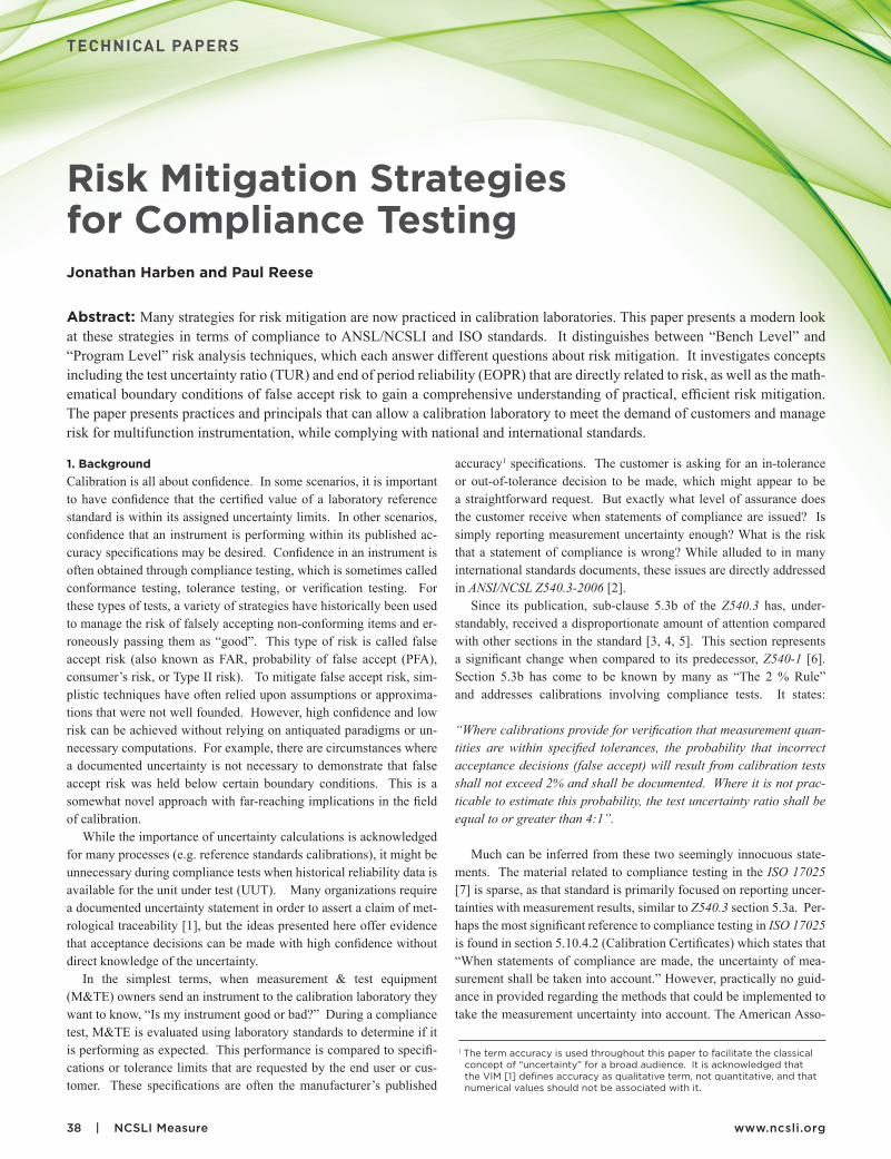
Figure 1. Five possible bench level calibration scenarios.

ciation of Laboratory Accreditation (A2LA) further clarifies the requirements associated with this concept in R205 [8]:

“When parameters are certified to be within specified tolerance, the associated uncer-tainty of the measurement result is properly taken into account with respect to the toler-ance by a documented procedure or policy established and implemented by the labora-tory that defines the decision rules used by the laboratory for declaring in or out of tol-erance conditions”.2

Moreover, the VIM [1] has recently added a new “Note 7” to the definition of metrologi-cal traceability. This note reiterates that the International Laboratory Accreditation Coop-eration (ILAC) requires a documented mea-

surement uncertainty for any and all claims of metrological traceability. However, simply re-porting the uncertainty along with a measure-ment result may not satisfy customer require-ments where compliance tests are desired. Without having a quantifiable control limit such as false accept risk, this type of reporting imparts unknown risks to the customer.

The methods presented in this paper pro-vide assurance that PFA risks are held be-low a specified maximum permissible value (2 %) without direct knowledge of the un-certainty. However, they may not satisfy the strict language of national and international documents, which appear to contain an im-plicit requirement to document measurement uncertainties for all calibrations.

Where compliance tests are involved, the intent of the uncertainty requirements may (arguably) be to allow an opportunity to evaluate the risks associated with pass/fail compliance decisions. If this is indeed the intent, then the ideas presented here can provide the same opportunity for evalua-tion without direct knowledge of the uncer-tainty. Because considerable effort is often required to generate uncertainty statements, it is suggested that accreditation bodies ac-cept the methods described in this paper as an alternative solution for compliance testing.

2. taking the uncertaintyInto account

What does it mean to “take the uncertainty into account” and why it is necessary? For an intuitive interpretation, refer to Fig. 1. Dur-ing a compliance test “on the bench”, what are the decision rules if uncertainty is taken into account? For example, during the calibration, the UUT might legitimately be observed to be in-tolerance. However, the observation could be misleading or wrong as illustrated in Fig. 1.

It is understood that all measurements are only estimates of the true value of the measur-and; this true value cannot be exactly known due to measurement uncertainty. In scenario #1, a reading on a laboratory standard volt-meter of 9.98 V can confidently lead to an in-tolerance decision (pass) for this 10 V UUT source with negligible risk. This is true due to sufficiently small uncertainty in the measure-ment process and the proximity of the mea-sured value to the tolerance limit. Likewise, a non-compliance decision (fail) resulting from scenario #5 can also be made with high confidence, as the measured value of 9.83 V is clearly out-of-tolerance. However, in sce-narios #2, #3, and #4, there is significant risk that a pass/fail decision will be incorrect.

authorsJonathan HarbenThe Bionetics CorporationM/S: ISC-6175Kennedy Space Center, FL 32899jonathan.p.harben@nasa.gov

Paul reeseCovidien, Inc.815 Tek DriveCrystal Lake, IL 60014paul.reese@covidien.com

2 The default decision rule is found in ILAC-G8:1996 [9], “Guidelines on Assessment and Reporting of Compliance with Specification”, section 2.5. With agreement from the customer, other decision rules may be used as provided for in this section of the requirements.

40 | NCSLI Measure www.ncsli.org

TECHNICAL PAPERS

In scenarios, #2, #3, & #4, this uncer-tainty makes it possible for the true value of the measurand to be either in or out of toler-ance. Consider scenario #3, where the UUT was observed at 9.90 V, exactly at the lower allowable tolerance limit. Under such condi-tions, there is a 50 % probability that either an in-tolerance or out-of-tolerance decision will be incorrect, barring any other information. In fact, even for standards with the lowest possible uncertainty, the probability of being incorrect will remain at 50 % in scenario #33. This concept of bench level risk is addressed in several documents [9, 10, 11, 12].

The simple analysis of the individual measurement results presented above is not directly consistent with the intent of “The 2 % rule” in Z540.3, although it still has application. Until now, our discussion has dealt exclusively with bench level analysis of measurement decision risk. That is, risk was predicated only on knowledge of the relationship between the UUT tolerance, the measurement uncertainty, and the observed measurement result made “on-the-bench”. However, the computation of false accept risk, for strict compliance with the 2 % rule in Z540.3, does not depend on any particular measurement, nor does it depend on its prox-imity to a given UUT tolerance limit. Instead, the 2 % rule in Z540.3 addresses the risk at the program level, prior to obtaining a mea-surement result. To understand both bench level and program level false accept risk, the intent underlying the 2 % rule and its relation-ship to TUR and EOPR4 must be examined. 3. the answer to two Different

QuestionsFalse accept risk describes the overall prob-ability of false acceptance when pass/fail decisions are made. False accept risk can be interpreted and analyzed at either the bench level or the program level [4]. Both risk lev-els are described in ASME Technical Report B89.7.4.1-2005 [13]. The ASME report refers to bench level risk mitigation as “controlling

the quality of individual workpieces”, while program level risk strategies are described as “controlling the average quality of work-pieces”. Bench level risk can be thought of as an instantaneous liability at the time of mea-surement, whereas program level risk speaks more to the average probability that incorrect acceptance decisions will be made based on historical data. These two approaches are related, but result in two answers to two dif-ferent questions. Meeting a desired quality objective requires an appropriate answer to an appropriate question, and ambiguity in the question itself can lead to different assump-tions regarding the meaning of false accept risk. Many international documents discuss only the bench level interpretation of risk, and require an actual measurement result to be available [9, 10, 11, 12]. These documents describe the most basic implementation of bench level risk, where no other “pre-mea-surement” state of knowledge exists. They address the instantaneous false accept risk associated with an acceptance decision for a single measured value, without the additional insight provided by historical data. This most basic of bench level techniques is sometimes called the confidence level method. How-ever, if “a-priori” data exists, a more rigor-ous type of bench-level analysis is possible using Bayesian methods. By employing prior knowledge of reliability data, Bayesian anal-ysis updates or improves the estimate of risk.

The Z540.3 standard, however, was in-tended to address risk at the program level [14]. When this standard requires “…the probability that incorrect acceptance deci-sions (false accept) will result from calibra-tion tests shall not exceed 2%..”, it might not be evident which view point is being ad-dressed, the bench level or the program lev-el. The implications of this were significant enough to prompt NASA to request interpre-tive guidance from the NCSLI 174 Standards Writing Committee [15]. It was affirmed that the 2 % false accept requirement applies to a “population of ‘like calibration sessions’ or ‘like measurement processes’ [14]. As such, Z540.3 section 5.3b does not directly address the probability of false accept to any single, discrete measurement result or individual workpiece and supports the program level view of risk prior to, and independent of, any particular measurement result.

In statistical terms, the 2 % rule refers to the unconditional probability of false accep-tance. In terms of program level risk, false

accept risk describes the overall or average probability of false acceptance decisions to the calibration program at large. It does not represent risk associated with any particular instrument. The 2 % rule speaks to the fol-lowing question: Given a historical collec-tion of pass/fail decisions at a particular test-point for a population of like-instruments (i.e. where the EOPR and TUR are known), what is the probability that an incorrect acceptance decision will be made during an upcoming test? Note that no measurement results are provided, and that the question is being asked before the scheduled measurement is ever made and the average risk is controlled for future measurements. Even so, the question can be answered as long as previous EOPR data on the UUT population is available, and if the measurement uncertainty (and thus TUR) is known. In certain circumstances, it is also possible to comply with the 2 % rule by bounding or limiting false accept risk us-ing either:

• EOPR data without knowledge of the measurement uncertainty.

• TUR without knowledge of EOPR data.

To understand how this is possible, a closer look at the relationship between false accept risk, EOPR, and TUR is helpful. 4. end of Period reliability (eOPr)EOPR is the probability of a UUT test-point being in-tolerance at the end of its normal calibration interval. It is sometimes known as in-tolerance probability and is derived from previous calibrations. In its simplest form, EOPR can be defined as

EOPR = Number of in-tolerance resultsTotal number of calibrations

. (1)

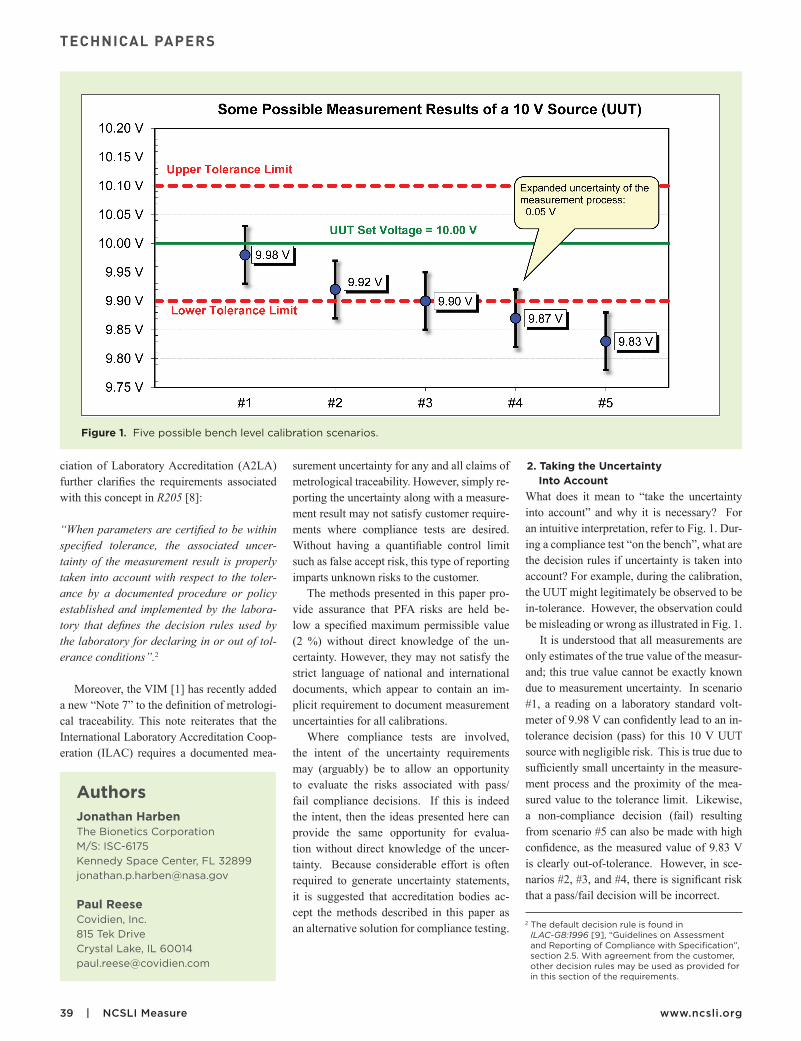
If prior knowledge tells us that a significant number of previous measurements for a pop-ulation of UUTs were very close to their tol-erance limits “as-received”, it can affect the false accept risk for an upcoming measure-ment. Consider Fig. 2 where two different model UUT voltage sources are scheduled for calibration, model A and model B. The five previous calibrations on model A’s have shown these units to be highly reliable; see Group A. Most often, they are well within their tolerance limits and easily comply with their specifications. In contrast, previous model B calibrations have seldom met their specifications; see Group B. Of the last five

3 Bayesian analysis can result in false accept risk other than 50 % in such instances, where the a priori in-tolerance probability (EOPR) of the UUT is known in addition to the measurement result and uncertainty.

4 The subject of measurement decision risk includes not only the probability of false-accept (PFA), but the probability of correct accept (PCA), probability of false reject (PFR) and the probability of correct reject (PCR). While false rejects can have significant economic impact to the calibration lab, the discussion in this paper is primarily limited to false accept risk.

41 | NCSLI Measure www.ncsli.org

TECHNICAL PAPERS

calibrations, two model B’s were recorded as being out-of-tolerance and one of them was “barely-in”. Therefore, making an in or out of tolerance decision will be a precari-ous judgment call, with a high probability of making a false accept decision.

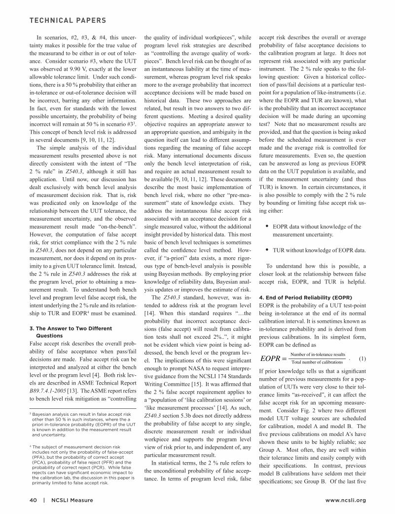
In Fig. 3, imagine the measurement result is not yet shown on the chart. If it was known ahead of time that this upcoming measure-

ment result would be near the tolerance limit, it can be seen that a false accept would indeed be more likely given the uncertainty of the measurement. The critically important point is this -- if the historical reliability data in-dicates that in-tolerance probability (EOPR) of the UUT is poor (up to a point5), the false accept risk increases.

The previous scenarios assume familiar-

ity with populations of similar instruments that are periodically recalibrated. But how can EOPR be reconciled when viewed from a “new” laboratory’s perspective? Can a

5 Graphs of EOPR vs. false-accept risk can reveal a perceived decrease in false-accept risk as the EOPR drops below certain levels. This is due to the large number of out-of-tolerance conditions that lie far outside the UUT tolerance limits. This is discussed later in this paper.

Figure 2. Previous historical measurement data can influence future false accept risk.

Figure 3. The possibility of a false accept for a measurement result.

42 | NCSLI Measure www.ncsli.org

TECHNICAL PAPERS

new laboratory open its doors for business and meet the 2 % false accept requirement of Z540.3 without EOPR data? The answer is “yes”. However, the new laboratory must employ bench level techniques, or techniques such as boundary condition methods or guardbanding. Such methods are described later in this paper. This same logic would ap-ply to an established laboratory that receives a new, unique instrument to calibrate for the first time. In the absence of historical data, other appropriate techniques and/or bench level methods must be employed.

If EOPR data or in-tolerance probability is important for calculating risk, several other questions are raised. For example, how good must the estimate of EOPR be before pro-gram level methods can be used to address false accept risk for a population of instru-ments? When is the collection of measure-ment data complete? What are the rules for updating EOPR in light of new evidence? Sharing or exchanging EOPR data between different laboratories has even been proposed with varying opinions. Acceptance of this generally depends upon the consistency of the calibration procedure used and the labo-ratory standards employed. The rules used to establish EOPR data can be subjective (for example, how many samples are avail-able, are first-time calibrations counted, are broken instruments included, are late calibra-tions included, and so on). Instruments can be grouped together by various classifica-tions, such as model number. For example, reliability data for the M&TE model and manufacturer level can be used to conserva-tively estimate the reliability of the M&TE test point. This is addressed in compliance Method 1 & 2 of the Z540.3 Handbook [16]. 5. test uncertainty ratioIt has been shown that EOPR can affect the false accept risk of calibration processes. However, test uncertainty ratio (TUR) is like-ly to be more familiar than EOPR as a metric of the “quality” of calibration. The preced-ing examples show that a lower uncertainty generally reduces the likelihood of a false accept decision. The TUR has historically been viewed as the uncertainty or tolerance of the UUT in the numerator divided by the uncertainties of the laboratory’s measurement standard(s) in the denominator [17]. A TUR greater than 4:1 was thought to indicate a ro-bust calibration process.

The TUR originated in the Navy’s Produc-

tion Quality Division during the 1950’s in an attempt to minimize incorrect acceptance decisions. The origins of the ubiquitous 4:1 TUR [18] assume a 95 % in-tolerance prob-ability for both the measuring device and the UUT. In those pre-computer days, these as-sumptions were necessary to ease the compu-tational requirements of risk analysis. Since then, manufacturers’ specifications have of-ten been loosely inferred to represent 2σ or 95 % confidence for many implementations of TUR, unless otherwise stated. In other words, it is assumed that all UUT’s will meet their specifications 95 % of the time (i.e. EOPR will be 95 %). Even if the calibration personnel did not realize it, they were relying on these assumptions to gain any utility out of the 4:1 TUR. However, is the EOPR for all M&TE really 95 %? That is, are all manufac-turers’ specifications based on two standard deviations of the product distribution? If they are not, then the time-honored 4:1 TUR will not provide the expected level of protection for the consumer.

While the spirit of Z540.3 is to move away from the reliance on TUR altogether, its use is still permitted if adherence to the 2 % rule is deemed “impracticable”. The use of the TUR is discouraged due to the many assumptions it relies on for controlling risk. However, given that the false accept risk computation requires the collection of EOPR data, the use of TUR might be perceived as an easy way for labs to circumvent the 2 % rule. Section 3.11 in Z540.3 redefines TUR as:

“The ratio of the span of the tolerance of a measurement quantity subject to calibration, to twice the 95% expanded uncertainty of the measurement process used for calibration”.

At first, this definition appears to be simi-lar to older definitions of TUR. The defini-tion implies that if the numerator, associated with the specification of the UUT, is a plus-or-minus (±) tolerance, the entire span of the tolerance must be included. However, this is countered by the requirement to multiply the 95 % expanded uncertainty of the measure-ment process in the denominator by a factor of two. The confidence level associated with the UUT tolerance is undefined. This quanda-ry is not new, as assumptions about the level of confidence associated with the UUT (nu-merator) have been made for decades.

There is, however, a distinct difference between the TUR as defined in Z540.3 and

previous definitions. This difference centers on the components of the denominator. In Z540.3, the uncertainty in the denominator is very specifically defined as the “uncertainty of the measurement process used in calibra-tion.” This definition has broader implica-tions than historical definitions because it includes elements of the UUT performance (for example, resolution and process repeat-ability) in the denominator. Many laborato-ries have long assumed that the uncertainty of the measurement process, as it relates to the denominator of TUR, should encompass all aspects of the laboratory standards, envi-ronmental effects, measurement processes, etc., but not the aspects of the UUT. His-torically, the TUR denominator reflected the capability of the laboratory to make highly accurate measurements, but this “capability” was sometimes viewed in the abstract sense, and was independent of any aspects of the UUT. The redefined TUR in the Z540.3 in-cludes everything that affects a laboratory’s ability to accurately perform a measurement on a particular device in the expanded uncer-tainty, including UUT contributions. This was reiterated to NASA in another response from the NCSLI 174 Standards Writing Com-mittee [19].

The “new” definition of TUR is meant to serve as a single simplistic metric for evaluat-ing the plausibility of a proposed compliance test with regard to mitigating false accept risk. No distinction is made as to where the risk originates, it could originate with either the UUT or the laboratory standard(s). A low TUR does not necessarily imply that the laboratory standards are not “good enough”. It might indicate, however, that the measure-ment cannot be made without significant false accept risk due to the limitations of the UUT itself. Such might be the case if the accuracy specification of a device is equal to its resolu-tion or noise floor. This can prevent a reliable pass/fail decision from being made.

When computing TUR with confidence levels other than 95 %, laboratories have sometimes attempted to convert the UUT specifications to ±2σ before dividing by the expanded uncertainty (2σ) of the measure-ment process. Or, equivalently, UUT specs were converted to ±1σ for division by the standard uncertainty (1σ) of the measure-ment process. Either way, this was believed by some to provide a more useful “apples-to-apples” ratio for the TUR. Efforts to develop an equivalent or normalized TUR have been

43 | NCSLI Measure www.ncsli.org

TECHNICAL PAPERS

documented by several authors [18, 20, 21, 22]. However, the integrity of a TUR depends upon the level of effort and honesty demon-strated by the manufacturer when assigning accuracy specifications to their equipment. It is important to know if the specifications are conservative and reliable, or if they were produced by a marketing department that was motivated by other factors.

6. understanding Program Level False

accept riskInvestigating the dependency of false accept risk on EOPR and TUR is well worth the ef-fort involved. The reader is referred to several papers that provide an excellent treatment of the mathematics behind the risk requirements at the program level [3, 4, 23, 24, 25]. These publications and many others build upon the seminal works on measurement decision risk by Eagle, Grubbs, Coon, & Hayes [18, 26, 27] and should be considered required reading.

This discussion is more conceptual in nature, but a brief overview of some funda-mental principles is useful. As stated earlier, M&TE tolerance limits are often set by the manufacturer’s accuracy specifications. The device may be declared in-tolerance if the UUT is observed to have a calibration result eobs that is within the tolerance limits L. This can be written as – L ≤ eobs ≤ L. The observed calibration result eobs is related to the actual or true UUT error euut and the measurement pro-cess error estd by the equation eobs = euut + estd. Note that the quantity euut is the parameter be-ing sought when a calibration is performed, but eobs is what is obtained from the measure-ment. The value of euut is always an estimate due to the possibility of measurement process errors estd described by uncertainty U95. It is not possible to determine euut exactly.

Errors (such as euut and estd), as well as measurement observations (such as eobs), are quantities represented by random variables and characterized by probability density functions. These distributions represent the relative likelihood of any specific error (euut and estd) or measurement observation (eobs) actually occurring. They are most often of the Gaussian form or normal distribution and are described by two parameters, a mean or average µ, and a standard deviation σ. The standard deviation is a measure of the vari-ability or spread in the values from the mean. The mean µ of all the possible error values will be zero, which assumes systematic ef-fects have been corrected. Real-world mea-

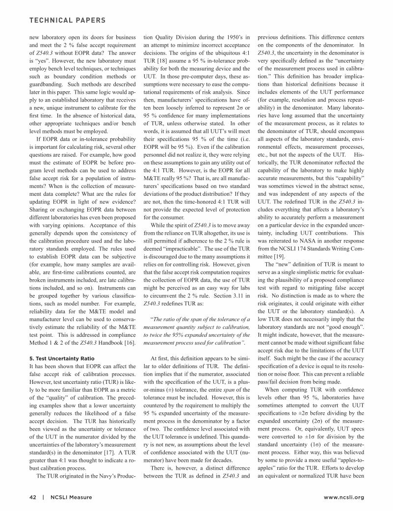
Figure 4. The probability density of possible measurement results.

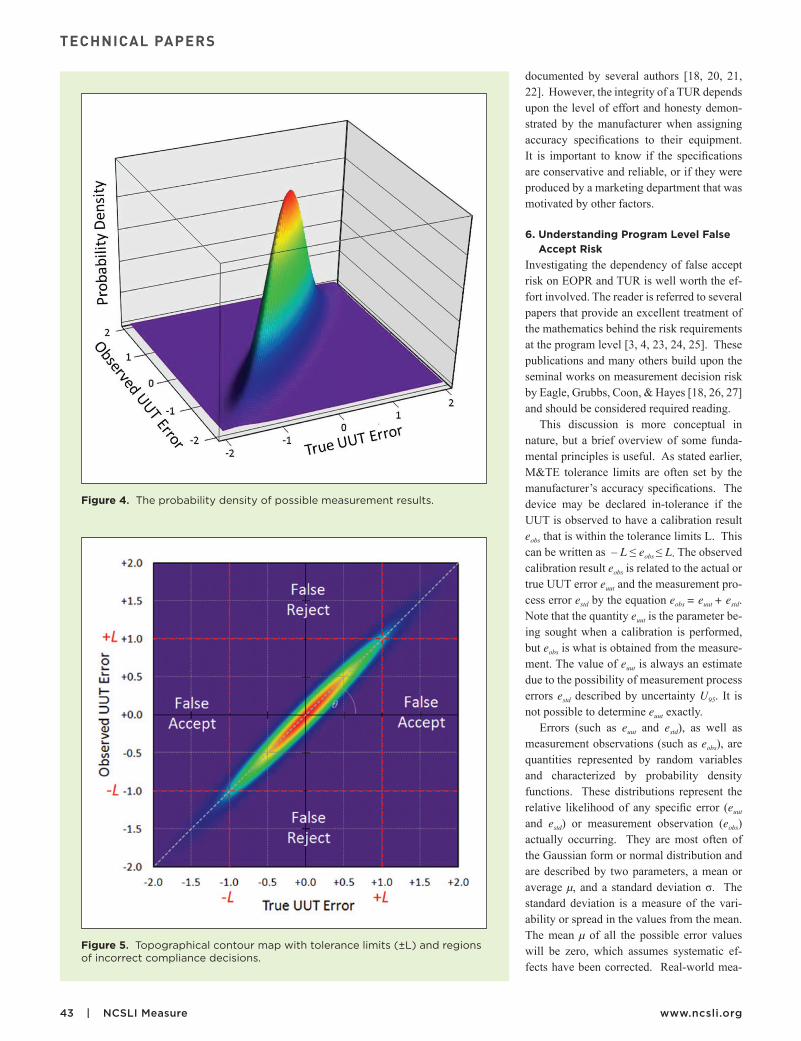
Figure 5. Topographical contour map with tolerance limits (±L) and regions of incorrect compliance decisions.

44 | NCSLI Measure www.ncsli.org

TECHNICAL PAPERS

surements are a function of both (𝑒𝑢𝑢𝑡) charac-terized by the UUT performance σuut and the measurement eobs with associated uncertainty 𝜎𝑠𝑡𝑑, where s obs = s uut + s std . The relative like-lihood of all possible measurement results is represented by the two dimensional surface area created by the joint probability distribu-tion given by 𝑝(𝑒𝑢𝑢𝑡, eobs) = 𝑝(𝑒𝑢𝑢𝑡) 𝑝(𝑒std). Fig-ures 4 and 5 illustrate the concept of prob-ability density of measurement and represent the relative likelihood of possible measure-ment outcomes given the variables TUR and EOPR. It is assumed that measurement un-certainty and the UUT distribution follow a normal or Gaussian probability density func-tion, yielding a bivariate normal distribution. Figure 5 is a top-down perspective of Fig. 4, when viewed from above.

The height, shape, and angle of the joint probability distribution change as a function of input variables TUR and EOPR. The dy-namics of this are critical, as they define the amount of risk for a given measurement sce-nario. The nine regions in Fig. 5 are defined by two-sided symmetrical tolerance limits. Risk is the probably of a measurement oc-curring in either the false accept regions or the false reject regions. Computing an actual numeric value for the probability (PFA or PFR) involves integrating the joint probabil-ity density function over the appropriate two dimensional surface areas (regions) defined by the limits stated below. Incorrect (false) acceptance decisions are made when euut > |L| and – L ≤ eobs ≤ L. In this case, the UUT is truly out of tolerance, but is observed to be in tolerance. Likewise incorrect (false) re-ject decisions are made when eobs >|L| and – L ≤ euut ≤ L, or where the UUT is observed to be out of tolerance, but is truly in tolerance. Integration over the entire joint probability region will yield a value of 1, as would be expected. This encompasses 100 % of the volume under the surface of Fig. 4. When the limits of integration are restricted to the two false accept regions shown in Fig. 5, a small portion of the total volume is computed which represents the false accept risk as a percentage of that total volume.

In the ideal case, if the measurement un-certainty was zero, the probability of mea-surement errors estd occurring would be zero. The measurements would then perfectly re-flect the behavior of the UUT and the distri-bution of possible measurement results would be limited to the distribution of actual UUT errors. That is, 𝑝(𝑒obs) would equal 𝑝(𝑒uut)

and the graph in Fig. 5 would collapse to a straight line at a 45° angle and the width in Fig. 4 would collapse to a simple two dimen-sional surface with zero volume. However, since real-world measurements are always hindered by the probability of errors, obser-vations do not perfectly reflect reality and risk results. In this case, the angle is given by tan(q ) = s obs

s uut

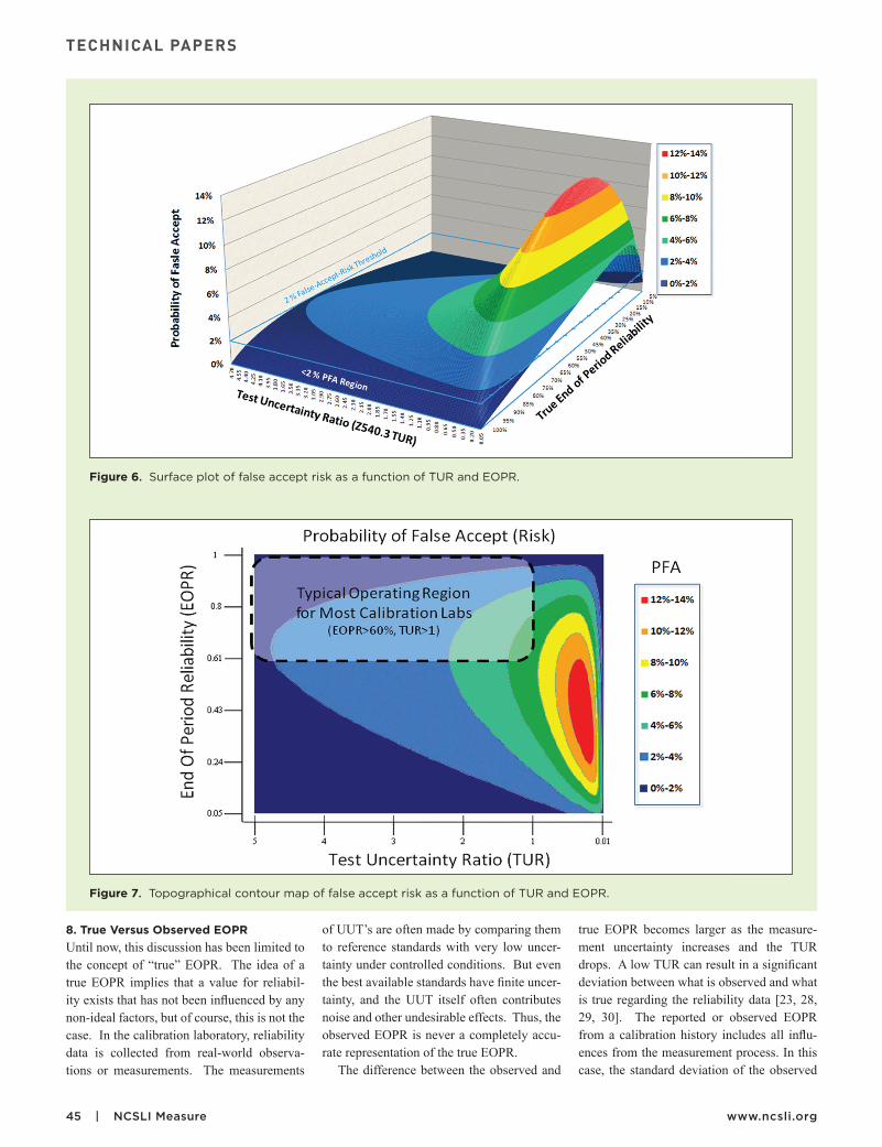
, where 45 ≤ 𝜃 ≤ 90. 7. efficient risk mitigationIn order for a calibration laboratory to comply with Z540.3 (5.3b), the program level PFA must not exceed 2 % and must be document-ed. However, computing an actual value for PFA is not necessarily required when demon-strating compliance with the 2 % rule. To un-derstand this, consider that the boundary con-ditions of PFA can be investigated by varying the TUR and EOPR over a wide range of val-ues and observing the resultant PFA. This is best illustrated by a three dimensional surface plot, where the x and y axis represent TUR and EOPR, and the height of the surface on the z-axis represents PFA (Fig. 6 and 7).

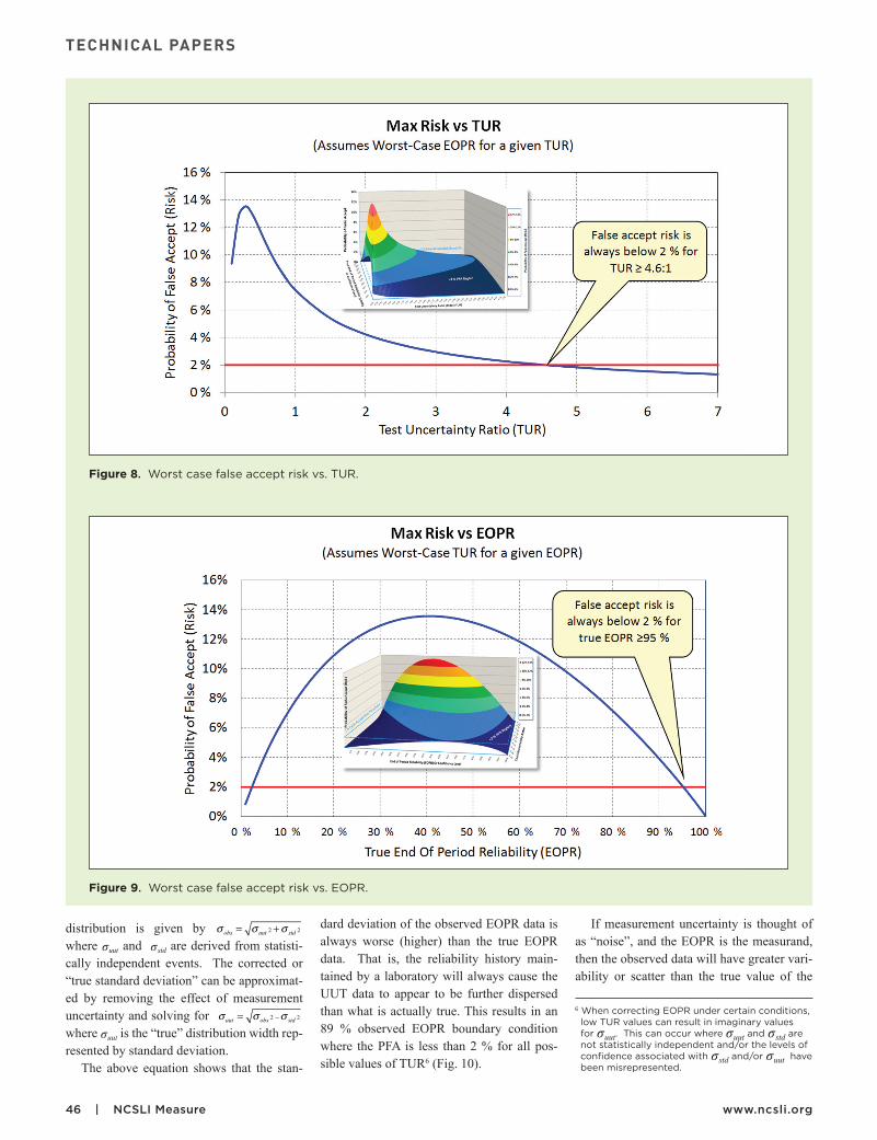
This surface plot combines both aspects affecting false accept risk into one visual representation that illustrates the relationship between the variables TUR and EOPR. One curious observation is that the program level PFA can never be greater than 13.6 % for any combination of TUR and EOPR. The maxi-mum value of 13.6 % occurs when the TUR is approximately 0.3:1 and the EOPR is 41 %. Any change, higher or lower, for either the TUR or EOPR will result in a PFA lower than 13.6 %.

One particularly useful observation is that, for all values of EOPR, the PFA never ex-ceeds 2 % when the TUR is above 4.6:1. In Figures 6 and 7, the darkest blue region of the PFA surface is always below 2 %. Even if the TUR axis in the above graph were extended to infinity, the darkest blue PFA region would continue to fall below the 2 % threshold. Cal-ibration laboratory managers will find this to be an efficient risk mitigation technique for compliance with Z540.3. The burden of col-lecting, analyzing, and managing EOPR data can be eliminated when the TUR is greater than 4.6:1.

This concept can be further illustrated by rotating the perspective (viewing angle) of the surface plot in Fig. 6, allowing the two dimensional maximum outer-envelope or boundary to be easily viewed. With this per-spective, PFA can be plotted only as a func-

tion of TUR (Fig. 8). In this instance, the worst-case EOPR is used whereby the maxi-mum PFA is produced for each TUR.

The left-hand side of the graph in Fig. 8 might not appear intuitive at first. Why would the PFA suddenly decrease as the TUR drops below 0.3:1 and approaches zero? While a full explanation is beyond the scope of this paper, the answer lies in the number of items rejected (falsely or otherwise) when an extremely low TUR exists. This causes the angle 𝜃 of the joint probability distribution to rotate counter-clockwise away from the ideal 45° line, shifting areas of high density away from the false accept regions illustrated in Fig. 5. For a very low TUR, there are indeed very few false accepts and very few correct rejects. The outcome of virtually all mea-surement decisions is then distributed over the correct accept and false reject regions as 𝜃 approaches 90°. It would be impractical for a calibration laboratory to operate under these conditions, although false-accepts would be exceedingly rare.

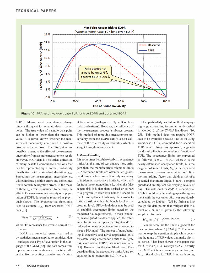
Examining the boundary conditions of the surface plot also reveals that the PFA is always below 2 % where the true EOPR is greater than 95 %. This is true even with ex-tremely low TUR’s (even below 1:1). Again, if the perspective of the PFA surface plot in Fig. 6 is properly rotated, a two dimensional outer-envelope is produced whereby PFA can be plotted only as a function of EOPR (Fig. 9). The worst-case TUR is used for each and every point of the Fig. 9 curve, maximizing the PFA, and illustrating that knowledge of the TUR is not required.

As was the case with a low TUR, a simi-lar phenomenon is noted on the left-hand side of the graph in Fig. 9; the maximum PFA decreases for true EOPR values below 41 %. As the EOPR approaches zero on the left side, most of the UUT values lie far outside of the tolerance limits. When the values are not in close proximity to the tolerance limits, the risk of falsely accepting an item is low. Likewise on the right-hand side of the graph, where the EOPR is very good (near 100 %), the false accept risk is low. Both ends of the graph represent areas of low PFA because most of the UUT values have historically been found to lie far away from the tolerance limits. The PFA is highest, in the middle of the graph, where EOPR is only moderately poor, and where much of the data is near the tolerance limits.

45 | NCSLI Measure www.ncsli.org

TECHNICAL PAPERS

8. true Versus Observed eOPrUntil now, this discussion has been limited to the concept of “true” EOPR. The idea of a true EOPR implies that a value for reliabil-ity exists that has not been influenced by any non-ideal factors, but of course, this is not the case. In the calibration laboratory, reliability data is collected from real-world observa-tions or measurements. The measurements

of UUT’s are often made by comparing them to reference standards with very low uncer-tainty under controlled conditions. But even the best available standards have finite uncer-tainty, and the UUT itself often contributes noise and other undesirable effects. Thus, the observed EOPR is never a completely accu-rate representation of the true EOPR.

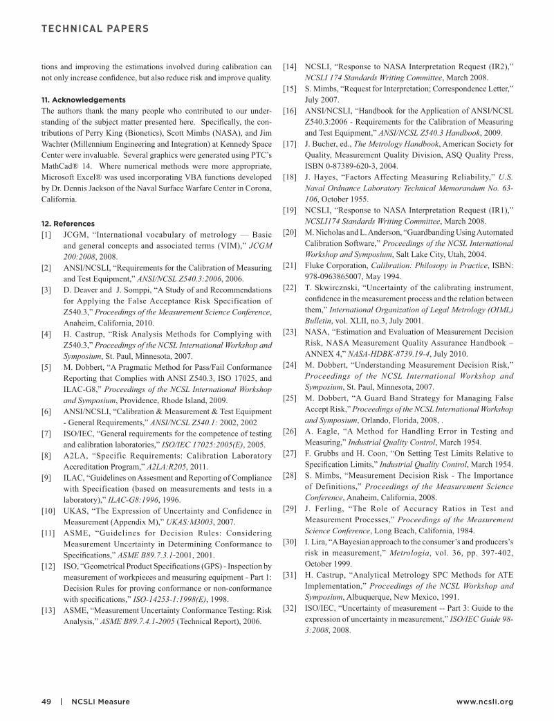
The difference between the observed and

true EOPR becomes larger as the measure-ment uncertainty increases and the TUR drops. A low TUR can result in a significant deviation between what is observed and what is true regarding the reliability data [23, 28, 29, 30]. The reported or observed EOPR from a calibration history includes all influ-ences from the measurement process. In this case, the standard deviation of the observed

Figure 6. Surface plot of false accept risk as a function of TUR and EOPR.

Figure 7. Topographical contour map of false accept risk as a function of TUR and EOPR.

46 | NCSLI Measure www.ncsli.org

TECHNICAL PAPERS

distribution is given by s obs = s uut 2 + s std 2 where 𝜎𝑢𝑢𝑡 and 𝜎std are derived from statisti-cally independent events. The corrected or “true standard deviation” can be approximat-ed by removing the effect of measurement uncertainty and solving for s uut = s obs 2 - s std 2 where 𝜎uut is the “true” distribution width rep-resented by standard deviation.

The above equation shows that the stan-

dard deviation of the observed EOPR data is always worse (higher) than the true EOPR data. That is, the reliability history main-tained by a laboratory will always cause the UUT data to appear to be further dispersed than what is actually true. This results in an 89 % observed EOPR boundary condition where the PFA is less than 2 % for all pos-sible values of TUR6 (Fig. 10).

If measurement uncertainty is thought of as “noise”, and the EOPR is the measurand, then the observed data will have greater vari-ability or scatter than the true value of the

6 When correcting EOPR under certain conditions, low TUR values can result in imaginary values for 𝜎uut. This can occur where 𝜎uut and 𝜎std are not statistically independent and/or the levels of confidence associated with 𝜎std and/or 𝜎uut have been misrepresented.

Figure 8. Worst case false accept risk vs. TUR.

Figure 9. Worst case false accept risk vs. EOPR.

47 | NCSLI Measure www.ncsli.org

TECHNICAL PAPERS

EOPR. Measurement uncertainty always hinders the quest for accurate data; it never helps. The true value of a single data point can be higher or lower than the measured value, it is never known whether the mea-surement uncertainty contributed a positive error or negative error. Therefore, it is not possible to remove the effect of measurement uncertainty from a single measurement result. However, EOPR data is a historical collection of many pass/fail compliance decisions that can be represented by a normal probability distribution with a standard deviation 𝜎obs. Sometimes the measurement uncertainty 𝜎std will contribute positive errors and sometimes it will contribute negative errors. If the mean of these estd errors is assumed to be zero, the effect of measurement uncertainty on a popu-lation of EOPR data can be removed as previ-ously shown. The inverse normal function is used to estimate 𝜎obs from observed EOPR data [31]

whether the measurement uncertainty contributed a positive error or negative error. Therefore, it is not possible to remove the effect of measurement uncertainty from a single measurement result. However, EOPR data is a historical collection of many pass/fail compliance decisions that can be represented by a normal probability distribution with a standard deviation . Sometimes the measurement uncertainty will contribute positive errors and sometimes it will contribute negative errors. If the mean of these errors is assumed to be zero, the effect of measurement uncertainty on a population of EOPR data can be removed as previously shown. The inverse normal function is used to estimate from observed EOPR data [31]

( ) , (2)

where -1 represents the inverse normal distribution.

EOPR is a numerical quantity arrived at by statistical means applied to empirical data – analogous to a Type A evaluation in the language of the GUM [32]. The data comes from repeated measurements made over time rather than from accepting manufacturers’ claims at face value (analogous to Type B or heuristic evaluations). However, the influence of the measurement process is always present. This method of removing measurement uncertainty from the EOPR data is a best estimate of the true reality or reliability which is sought through measurement. 9. Guardbanding

It is sometimes helpful to establish acceptance limits A at the time-of-test that are more stringent than the manufacturers tolerance limits L. Acceptance limits are often called guardband limits or test-limits. It is only necessary to implement acceptance limits A, which differ from the tolerance limits L, when the false accept risk is higher than desired or as part of a program to keep risk below a specified level. Acceptance limits may be chosen to mitigate risk at either the bench level or the program level. PFA calculations may be used to establish acceptance limits based on the mandated risk requirements. In most instances, where guard bands are applied, the tolerance limits are temporarily “tightened” or reduced to create acceptance limits needed to meet a PFA goal. The subject of guardbanding is extensive and novel approaches exist for establishing acceptance limits to mitigate risk, even where EOPR data is not available [25]. However, in the simplified case of no guardbanding, the acceptance limits A are set equal to the tolerance limits L (A = L).

One particularly useful method employing a guardbanding technique is described in Method 6 of the Z540.3 Handbook [16, 25]. This method does not require EOPR data to be available because it relies on using worst-case EOPR, computed for a specified TUR value. Using this approach, a guardband multiplier is computed as a function of TUR. The acceptance limits are expressed as follows: , where is the newly established acceptance limits, is the original tolerance limits, is the expanded measurement process uncertainty, and is the multiplying factor that yields a risk of a specified maximum target. Figure 11 graphs guardband multipliers for varying levels of risk. The risk level for Z540.3 is specified at 2 % but could vary depending upon the agreement with the customer. was previously calculated by Dobbert [25] by fitting a line though the data points that mitigate risk to a level of 2 % and is given by the following simplified formula

(2)

where Φ-1 represents the inverse normal dis-tribution.

EOPR is a numerical quantity arrived at by statistical means applied to empirical data – analogous to a Type A evaluation in the lan-guage of the GUM [32]. The data comes from repeated measurements made over time rath-er than from accepting manufacturers’ claims

at face value (analogous to Type B or heu-ristic evaluations). However, the influence of the measurement process is always present. This method of removing measurement un-certainty from the EOPR data is a best esti-mate of the true reality or reliability which is sought through measurement.

9. GuardbandingIt is sometimes helpful to establish acceptance limits A at the time-of-test that are more strin-gent than the manufacturers tolerance limits L. Acceptance limits are often called guard-band limits or test-limits. It is only necessary to implement acceptance limits A, which dif-fer from the tolerance limits L, when the false accept risk is higher than desired or as part of a program to keep risk below a specified level. Acceptance limits may be chosen to mitigate risk at either the bench level or the program level. PFA calculations may be used to establish acceptance limits based on the mandated risk requirements. In most instanc-es, where guard bands are applied, the toler-ance limits are temporarily “tightened” or reduced to create acceptance limits needed to meet a PFA goal. The subject of guardband-ing is extensive and novel approaches exist for establishing acceptance limits to mitigate risk, even where EOPR data is not available [25]. However, in the simplified case of no guardbanding, the acceptance limits A are set equal to the tolerance limits L (A = L ).

One particularly useful method employ-ing a guardbanding technique is described in Method 6 of the Z540.3 Handbook [16, 25]. This method does not require EOPR data to be available because it relies on using worst-case EOPR, computed for a specified TUR value. Using this approach, a guard-band multiplier is computed as a function of TUR. The acceptance limits are expressed as follows: A = L – MU95 , where A is the newly established acceptance limits, L is the original tolerance limits, U95 is the expanded measurement process uncertainty, and M is the multiplying factor that yields a risk of a specified maximum target. Figure 11 graphs guardband multipliers for varying levels of risk. The risk level for Z540.3 is specified at 2 % but could vary depending upon the agree-ment with the customer. M2% was previously calculated by Dobbert [25] by fitting a line though the data points that mitigate risk to a level of 2 % and is given by the following simplified formula

M 2% = 1.04 - e0.38 ln(TUR)-0.54. (3) (3)

It can be seen that the line is a good fit for the condition where 1 ≤ TUR ≤ 15. The intent was to keep the equation simple while cover-ing the range of TUR values that make physi-cal sense. It has been shown in this paper that for TUR ≥ 4.6, PFA is always < 2 %. To verify that TUR = 4.6 is a boundary condition, set M2% = 0 and solve for TUR. It is worth noting

Figure 10. PFA assumes worst case TUR for true EOPR and observed EOPR.

48 | NCSLI Measure www.ncsli.org

TECHNICAL PAPERS

that, for ≥ 4.6, the multiplier M2% is < 0. This implies that a calibration lab could actually increase the acceptance limits A beyond the UUT tolerances L and still comply with the 2 % rule. While not a normal operating proce-dure for most calibration laboratories, setting guard band limits outside the UUT tolerance limits is possible while maintaining compli-ance with the program level risk requirement of Z540.3. In fact, laboratory policies often require items to be adjusted back to nominal for observed errors greater than a specified portion of their allowable tolerance limit L.

10. Conclusion and summaryOrganizations must determine if risk is to be controlled for individual workpieces at the bench level, or mitigated for the population of items at the program level7. Computation of PFA at the program level requires the integra-tion of the joint probability density function. The input variables to these formulas can be reduced to EOPR and TUR. The 2 % PFA maximum boundary condition, formed by ei-ther a 4.6:1 TUR or an 89 % observed EOPR, can greatly reduce the effort required to man-age false accept risk for a significant portion of the M&TE submitted for calibration. Ei-ther or both boundary conditions can be lev-eraged depending on the available data, pro-viding benefit to practically all laboratories. However, there will still be instances where the TUR is lower than 4.6: 1 and the observed

EOPR is less than 89 %. In these instances, it is still possible for the PFA to be less than 2 %. A full PFA computation is required to show the 2 % requirement has not been ex-ceeded. However, other techniques can be employed to ensure that the PFA is held below 2 % without an actual computation.

There are six methods listed in the Z540.3 Handbook for complying with the 2 % false accept risk requirement [16]. These methods encompass both program level and bench level risk techniques. This paper has specifi-cally focused on some efficient approaches for compliance with the 2 % rule, but it does not negate the use of other methods nor imply that the methods discussed here are necessar-ily the best. The basic strategies outlined here for handling risk without rigorous computa-tion of PFA are:

• Analyze EOPR data. This will most like-ly be done at the instrument-level, as op-posed to the test-point level, depending on data collection methods. If the observed EOPR data meets the required level of 89 %, then the 2 % PFA rule has been satisfied.

• If this is not the case, then further analysis is needed and the TUR must be determined at each test point. If the analysis reveals that the TUR is greater than 4.6:1, no further action is neces-sary and the 2 % PFA rule has been met.

• If neither the EOPR nor TUR threshold is met, a Method #6 guardband can be applied.

Compliance with the 2 % rule can be ac-complished by either calculating PFA and/or limiting its probability to less than 2% by the methods presented above. If these methods are not sufficient, alternative methods of miti-gating PFA are available [16]. Of course, no amount of effort on the part of the calibration laboratory can force a UUT to comply with unrealistic expectations of performance. In some cases, contacting the manufacturer with this evidence may result in the issuance of revised specifications that are more realistic.

Assumptions, approximations, estima-tions, and uncertainty have always been part of metrology, and no process can guarantee that instruments will provide the desired ac-curacy, or function within their assigned tol-erances during any particular application or use. However, a well-managed calibration process can provide confidence that an in-strument will perform as expected and within limits. This confidence can be quantified via analysis of uncertainty, EOPR, and false ac-cept risk. Reducing the number of assump-

7 Bayesian analysis can be performed to determine the risk to an individual workpiece using both the measured value on the bench and program-level EOPR data to yield the most robust estimate of false accept risk [31].

Figure 11. Guardband multiplier for acceptable risk limits as a function of TUR.

49 | NCSLI Measure www.ncsli.org

TECHNICAL PAPERS

tions and improving the estimations involved during calibration can not only increase confidence, but also reduce risk and improve quality.

11. acknowledgementsThe authors thank the many people who contributed to our under-standing of the subject matter presented here. Specifically, the con-tributions of Perry King (Bionetics), Scott Mimbs (NASA), and Jim Wachter (Millennium Engineering and Integration) at Kennedy Space Center were invaluable. Several graphics were generated using PTC’s MathCad® 14. Where numerical methods were more appropriate, Microsoft Excel® was used incorporating VBA functions developed by Dr. Dennis Jackson of the Naval Surface Warfare Center in Corona, California.

12. references[1] JCGM, “International vocabulary of metrology — Basic

and general concepts and associated terms (VIM),” JCGM 200:2008, 2008.

[2] ANSI/NCSLI, “Requirements for the Calibration of Measuring and Test Equipment,” ANSI/NCSL Z540.3:2006, 2006.

[3] D. Deaver and J. Somppi, “A Study of and Recommendations for Applying the False Acceptance Risk Specification of Z540.3,” Proceedings of the Measurement Science Conference, Anaheim, California, 2010.

[4] H. Castrup, “Risk Analysis Methods for Complying with Z540.3,” Proceedings of the NCSL International Workshop and Symposium, St. Paul, Minnesota, 2007.

[5] M. Dobbert, “A Pragmatic Method for Pass/Fail Conformance Reporting that Complies with ANSI Z540.3, ISO 17025, and ILAC-G8,” Proceedings of the NCSL International Workshop and Symposium, Providence, Rhode Island, 2009.

[6] ANSI/NCSLI, “Calibration & Measurement & Test Equipment - General Requirements,” ANSI/NCSL Z540.1: 2002, 2002

[7] ISO/IEC, “General requirements for the competence of testing and calibration laboratories,” ISO/IEC 17025:2005(E), 2005.

[8] A2LA, “Specific Requirements: Calibration Laboratory Accreditation Program,” A2LA:R205, 2011.

[9] ILAC, “Guidelines on Assesment and Reporting of Compliance with Specification (based on measurements and tests in a laboratory),” ILAC-G8:1996, 1996.

[10] UKAS, “The Expression of Uncertainty and Confidence in Measurement (Appendix M),” UKAS:M3003, 2007.

[11] ASME, “Guidelines for Decision Rules: Considering Measurement Uncertainty in Determining Conformance to Specifications,” ASME B89.7.3.1-2001, 2001.

[12] ISO, “Geometrical Product Specifications (GPS) - Inspection by measurement of workpieces and measuring equipment - Part 1: Decision Rules for proving conformance or non-conformance with specifications,” ISO-14253-1:1998(E), 1998.

[13] ASME, “Measurement Uncertainty Conformance Testing: Risk Analysis,” ASME B89.7.4.1-2005 (Technical Report), 2006.

[14] NCSLI, “Response to NASA Interpretation Request (IR2),” NCSLI 174 Standards Writing Committee, March 2008.

[15] S. Mimbs, “Request for Interpretation; Correspondence Letter,” July 2007.

[16] ANSI/NCSLI, “Handbook for the Application of ANSI/NCSL Z540.3:2006 - Requirements for the Calibration of Measuring and Test Equipment,” ANSI/NCSL Z540.3 Handbook, 2009.

[17] J. Bucher, ed., The Metrology Handbook, American Society for Quality, Measurement Quality Division, ASQ Quality Press, ISBN 0-87389-620-3, 2004.

[18] J. Hayes, “Factors Affecting Measuring Reliability,” U.S. Naval Ordnance Laboratory Technical Memorandum No. 63-106, October 1955.

[19] NCSLI, “Response to NASA Interpretation Request (IR1),” NCSLI174 Standards Writing Committee, March 2008.

[20] M. Nicholas and L. Anderson, “Guardbanding Using Automated Calibration Software,” Proceedings of the NCSL International Workshop and Symposium, Salt Lake City, Utah, 2004.

[21] Fluke Corporation, Calibration: Philosopy in Practice, ISBN: 978-0963865007, May 1994.

[22] T. Skwircznski, “Uncertainty of the calibrating instrument, confidence in the measurement process and the relation between them,” International Organization of Legal Metrology (OIML) Bulletin, vol. XLII, no.3, July 2001.

[23] NASA, “Estimation and Evaluation of Measurement Decision Risk, NASA Measurement Quality Assurance Handbook – ANNEX 4,” NASA-HDBK-8739.19-4, July 2010.

[24] M. Dobbert, “Understanding Measurement Decision Risk,” Proceedings of the NCSL International Workshop and Symposium, St. Paul, Minnesota, 2007.

[25] M. Dobbert, “A Guard Band Strategy for Managing False Accept Risk,” Proceedings of the NCSL International Workshop and Symposium, Orlando, Florida, 2008, .

[26] A. Eagle, “A Method for Handling Error in Testing and Measuring,” Industrial Quality Control, March 1954.

[27] F. Grubbs and H. Coon, “On Setting Test Limits Relative to Specification Limits,” Industrial Quality Control, March 1954.

[28] S. Mimbs, “Measurement Decision Risk - The Importance of Definitions,” Proceedings of the Measurement Science Conference, Anaheim, California, 2008.

[29] J. Ferling, “The Role of Accuracy Ratios in Test and Measurement Processes,” Proceedings of the Measurement Science Conference, Long Beach, California, 1984.

[30] I. Lira, “A Bayesian approach to the consumer’s and producers’s risk in measurement,” Metrologia, vol. 36, pp. 397-402, October 1999.

[31] H. Castrup, “Analytical Metrology SPC Methods for ATE Implementation,” Proceedings of the NCSL Workshop and Symposium, Albuquerque, New Mexico, 1991.

[32] ISO/IEC, “Uncertainty of measurement -- Part 3: Guide to the expression of uncertainty in measurement,” ISO/IEC Guide 98-3:2008, 2008.