- - - - -

NASA TECHNICAL NOTE NASA TN D-8513

m ­-G --­-aF) -

z c

m 4 z

ON THE LOGARITHMIC-SINGULARITY CORRECTION I N THE KERNEL FUNCTION METHOD OF SUBSONIC LIFTING-SURFACE THEORY

C, Edward Lan and John E. Lamur

Ldngley Research Center Humpton, Va. 23665

N A T I O N A L A E R O N A U T I C S A N D SPACE A D M I N I S T R A T I O N W A S H I N G T O N , D. C. NOVEMBER 1977 /I

r

13

https://ntrs.nasa.gov/search.jsp?R=19780004093 2019-07-14T10:49:28+00:00Z

TECH LIBRARY KAFB, NM

-~ ­1. Report No. 2. Government Accession No. 3. Recipient's Catalog No.

- NASA TN D-8513 I 7 4. Title and Subtitle 1 5. Report Date

SURFACE THEORY

7. Authorb)

C. Edward Lan and John E . Lamar

9. Performing Organization Name and Address

NASA Langley Research Center Hampton, VA 23665

.­

12. Sponsoring Agency Name and Address

National Aeronautics and Space Administration Washington, DC 20 546

15. Supplementary Notes

C. Edward Lan: University of Kansas, Lawrence, Kansas. John E. Lamar: Langley Research Center.

._

16. Abstract

8. Performing Organization Report No. L-11142

10. Work Unit No.

505-06-14-01 11. Contract or Grant No.

13. Type of Report and Period Covered

Technical Note I

14. Sponsoring Agency Code

A new logarithmic-singularity correction factor is derived fo r use in kernel function methods associated with Multhopp's subsonic lifting-surface theory. Because of the fo rm of the factor, a relation has been formulated between the numbers of chordwise and spanwise control points needed fo r good accuracy. This formulation is developed and discussed. Numerical resul ts are given to show the improvement of the computation with the new cor­rection factor.

17. Key-Words (Suggested by Author(s) 1 18. Distribution Statement

Lifting- surface theory Unclassified - Unlimited Subsonic Logarithmic-singularity correction Control-point c r i t e r i a Subject Category 02

.__ - _ - _ 19. Security Classif. (of this report1 20. Security Classif. (of this page)

Unclassified I Unclassified $4.50 - .

For sale by the National Technical Information Service, Springfield, Virginia 22161

I

I

ON THE LOGARITHMIC-SINGULARITY CORRECTION IN

THE KERNEL FUNCTION METHOD O F SUBSONIC

LIFTING-SURFACE THEORY

C. Edward Lan* and John E. Lamar Langley Research Center

SUMMARY

A new logarithmic-singularity correction factor is derived fo r use in kernel func­tion methods associated with Multhopp's subsonic lifting-surface theory. Because of the form of the factor, a relation has been formulated between the numbers of chordwise and spanwise control points needed fo r good accuracy. This formulation is developed and discussed. Numerical resul ts are given to show the improvement of the computation with the new correction factor.

INTRODUCTION

There are various kinds of singularities which arise in the kernel function methods of the lifting-surface theory. Since Multhopp published his method in 1950 (ref. l), much effort has been expended in obtaining an accurate accounting of these singularities. The singularities a r e associated with: (1) the mathematical modeling of the lift potential of a wing surface (i.e., doublets) and the resulting downwash produced by them as calculated in the analytical o r numerical spanwise integration over the lifting surface, (2) leading-edge pressures , and (3) changes in wing sweep a t the apex o r along the span (refs. 2 and 3).

Singularities associated with wing sweep are not given special treatment (i.e., special pressure modes), but instead Multhopp's procedure f o r rounding the leading and trailing edges in the vicinity of the affected regions is used (ref. 1). Leading-edge pres­su re singularities are expected because of the modes assumed, but they add to the first singularity problem listed and are treated in the context of this problem. The first singu­lari ty is the main subject considered herein.

The spanwise integration over the lifting surface generally has associated with it a logarithmic-type singularity t e rm at some spanwise position which in a purely numerical

*University of Kansas, Lawrence, Kansas.

treatment can lead to significant e r ro r s . To minimize these e r ro r s , the usual procedure is to separate the logarithmic t e rm and evaluate it to provide a "correction" to the 4 remainder of the integral. (Refs. 1and 4 are examples.) The t e rm which resu l t s is I

icalled the logarithmic-singularity correction (LSC). This approach was introduced by I

Multhopp in reference 1 (used later by others in refs. 2 to 9) along with a procedure fo r L

I

the LSC calculation. Improvements in the computational procedure have been formu- J I

lated by Mangler and Spencer (ref. 9) and Zandbergen, Labrujere, and Wouters (ref. 2). However, the most commonly used correction has a serious deficiency which arises because the correction t e rm consists only of the leading te rm of a correction series

B4Iwhich diverges as the chordwise control points approach the leading and trailing edges.

The exclusion of the high-order correction terms, logarithmic in nature, in this diver­

gent series has been credited by Jordan (ref. 8) as the main cause of significant e r r o r s

in some existing lifting-surface methods when the number of chordwise control points is increased. Jordan (ref. 8), Wagner (ref. 5), and Medan (ref. 3) have advocated the use of wing-edge control points for better accuracy in the solution. These wing-edge control points are known to be associated with algebraic, instead of logarithmic, singularity cor­

rections. However, even if wing-edge control points are used, the logarithmic correction factors which are needed for interior control points are sti l l inaccurate near the edges.

Another feature of existing kernel function methods is that the relation between numbers of chordwise and spanwise control points used to obtain a reliable solution has been empirical, derived by applying the theory to a limited number of planforms (ref. 7). However, experience indicates that this empirical relation is not applicable to a rb i t ra ry combinations of configurations and Mach number. It is in f ac t highly dependent on plan-fo rm and Mach number.

In this report , a method of obtaining a convergent correction series is presented and the leading t e rm of such a series is derived. Better convergence characterist ics of a modified Multhopp's method are illustrated when the new correction factor is used. In addition, a general relation governing numbers of chordwise and spanwise control points is derived and demonstrated to provide accurate solutions for arbi t rary planar planforms.

Some details of the development are given in appendixes A and By and implementa­tion of the analysis is given in appendix C.

SYMBOLS I

A = J(1 - x)2+ Y2

B = \/x2+ Y2

2

b wing span, equal to 2 in this report

bvv’bvn Multhopp’s quadrature weighting factors defined in equation (B21)

‘D,ii ra t io of near-field to far-field vortex drag ‘D,i

overall wing lift-curve slopeLo!

AcP lifting pressure coefficient

c1 constant to be determined

c(q),c(y) streamwise half-chord at q and y, respectively, nondimensionalized

by b/2

‘av average chord

E (k) complete elliptic integral of second kind

E ( d 4 incomplete elliptic integral of second kind

F(q,k) incomplete elliptic integral of first kind

Gj(C#I) function of C#I defined by equation (21)

h j jth chordwise loading function

Ij jth chordwise integral defined by equation (6)

Ijvv’Ij vn see equation (B22)

J1,J2 integrals defined by equations (15) and (16)

K(k) complete elliptic integral of first kind

k2 modulus of elliptic integrals squared, 1 - (A - B)2 4AB

3

C

complementary modulus of elliptic integrals squared, 1 - k2 - ( ~ + ~ ) 2 - 1-

4AB

see equation (B20)

k' at left and right wing tip, respectively

logarithmic component of Ij

f ree-s t ream Mach number

number of span stations where pressure modes are defined

number of chordwise control points a t each of m span stations

jth spanwise loading function

perturbation velocity in vertical direction nondimensionalized with respect to f ree-s t ream velocity

xO

x1

Y

X,Y streamwise and spanwise rectangular Cartesian coordinates nondimensiona­lized with respect to b/2 and associated with control-point locations

Xac aerodynamic center in fractions of reference chord and referenced to leading edge of reference chord, positive aft

4

small positive number

angle for locating control points along span, cos-l(q)

sweep angle, deg

Heuman's lambda function, equation (B3)

Root chord' also index in equation (23)taper ratio, Tip chord

rectangular Cartesian coordinates, nondimensionalized with respect to b/2, in x- and y-directions, respectively, and associated with pressure doublet locations

complete elliptic integral of third kind

incomplete elliptic integral of third kind

angular coordinate defined by X = 1 (1 - cos $)2

angular coordinate defined by X1 = -1 (1 - cos $1)2

= sin-l(A - B)

Subscripts:

le leading edge

n spanwise influencing station associated with particular 77 values

S chordwise control point associated with particular $ values

te trailing edge

V spanwise control point associated with particular y values

5

Abbreviation:

LSC logarithmic -singularity correction t e rm

The symbol f denotes finite -part integration.

MATHEMATICAL DEVELOPMENT

In linearized steady subsonic flow theory fo r a thin wing, the lifting pressure ACp is related to the downwash distribution on the wing surface through the following singular integral equation:

where the spanwise integration is defined by the finite-part concept. By introducing the new variables,

equation (1)becomes

In equation (3), the lifting pressure coefficient is usually approximated by

6

where

cos j$l + cos ( j + 1)$1

hj ($1) = sin $1

and

x1 = z1 (1 - cos $1)

It follows that equation (3) can be written as

where

1 cos j$l icos ( j + 1)$1 x - x, I s in $1

and

y = p y - 7 7 2 c(rl)

Now, it has been shown (ref. 1) that Ij

behaves like (y - q)2 ln(y - q ( near q = y. The factor (y - q)2 is canceled by the same factor in the denominator of equation (5), so that a logarithmic singularity at q = y appears. Accurate spanwise integration can be done only if this logarithmic singularity is carefully accounted for.

Mangler and Spencer (ref. 9) removed the logarithmic component of I., called Lj yJ

before performing the spanwise integration. This approach, also used here, leads to (es. (E31411

so that the te rm in the summation in equation (5) can be replaced with (eq. (B15))

7

Obviously, equation (8) involves L.J and therefore requires attention. A s q - y, Ij*(X,Y,q) var ies in X like I.(X,Y,y) and thusJ

i Logarithmic lim 1

Lj = component V--Y

- Ij@,Y,Y) = AI*of 3 (9) 1

so

1 cos j@l + cos (j + sin G1

It is observed that fo r small Y, the factors inside the brackets in this equation are small when X1 is not close to X and have significant magnitude only near X1 = X. For this reason, Multhopp (ref. 1) argued that for deriving the logarithmic correction term, it is reasonable to develop the function h j (eq. (4b)) into a Taylor series about the point X1 = X, or equivalently about @1= @. The result can be integrated exactly and then developed into a series for small Y to obtain the logarithmic components. Now, i t is obvious that h.J does not have a Taylor series expansion about the integration end points, X1 = 0 and X1 = 1. For example, by using equation (4c), the Taylor series expansion for ho is obtained as

This series obviously does not converge near X = 0 and X = 1. This nonconvergence of the series expansion is due to the presence of sin @1= 2/- in the

a

denominator of hj .

Therefore, a natural way to improve the series expansion is to expand only cos j+l + cos (j + 1)cbl as follows:

+ cos (j + 1 ) ~ $ ~12)- (xl - x) + o(xl - x ) 2

+I=+

where

gl(+) = cos j + + cos (j + l)+

and

g2(+) = -2 j s in j@+ (j + 1)sin (j + 1 ) ~ sin +

Hence, for small Y, equation (9) can be written as

9

! , i 1where equation (6) has been used and I!(X,Y,y) is the integral $(X,Y,y) with theJ

loading function expanded in accordance with equation (11). Obviously, the logarithmic correction t e rm comes only f rom the integrals expressed in equation (14). Note that if higher order correction t e r m s are desired, more t e rms should be retained in equa-

51

tion (11). The two integrals of equation (14) can be integrated exactly to give i

x - x1 J1 = lo1,/?; + d m ] dX1

= zk - AO(+,k) + B - kT2K(kg}2

J2 = l o1 x""1 1 - xl)

L +/+S-la1 Details of the integration are given in appendix A.

In appendix B, the LSC is derived; a summary of the derivation is given here. The relation between Y and k' is shown to be (eq. (B2))

Y2 = 4kt2X2(1 - X)2 (1+ - 8X(1 - Xg} + O(kT6)

Equation (17) shows that small k' implies always small Y. However, small Y does not always imply small k', depending on the value of X. It follows that it is more natural to develop J1 and J2 fo r small k', ra ther than fo r small Y, to find the loga­rithmic terms. This choice represents a deviation f rom Multhopp's original method. In developing equations (15) and (16) for small k', it is found that the logarithmic compo­* nents are (eqs. (B11) and (B10))

10

Logarithmic 2 c(y) sin @J

(y - q)2 dr7

In k' + O(kV3In k') (18)component = -sign (y - q ) -pOf J1

Logarithmic *(y - q)2 In k' + O(kf3 In k')component = -sign (y - q ) C(Y) s m @JOf J 2

It follows f rom equations (14) to (16) and (18) to (19) that for small Y the dominating logarithmic component of Ij can be written as (eq. (B12))

(y - q)2 In k' L j = -sign (y - q ) Ea drl G j ( d

C(Y)

where (eq. (E13))

It is shown in appendix B that equation (20) can be reduced to the conventional form by expanding dkf/dq and k' for small Y .

From the preceding development the first t e rm of equation (8) involves L.J

and contributes the following result to equation (5) (eq. (B16)):

where k i and k i are the values of k' at the left and the right wing tip, respectively. The notation has been made compatible with Multhopp's notation (ref. 1). Reference 7 gives a detailed explanation of the subscripts which have been introduced. For the second and third t e r m s of equation (8), Multhopp's method of integration can be applied by using the trigonometric interpolation formula of the type

m-1-2 -m

(qj~j)n sin hen s in xe X = l

(23)

11

m-1n=-­2

where 8, = - 7r -- and m is the number of spanwise integration stations over the 2 m + l

whole wing. The integration of the second and third t e r m s of equation (8) in equation (5) resul ts in (eq. (B19))

where the prime on the summation sign means that the t e rm with n = v is omitted f rom the summation. Combining equations (22) and (24)reduces equation (5) to the following equivalent algebraic equation:

where bvv and bm are Multhopp's quadrature weighting factors and are defined in appendix B for convenience. The detailed expression f o r dkL/dq is also given in appendix B. Equation (25) represents the new system of equations for determining the values of the loading function qj *

REGION O F VALIDITY FOR THE LSC

From the definition, it is known that

12

As indicated previously, the logarithmic-singularity correction t e rm (LSC) must be removed before accurate spanwise integration ac ross the second-order singularity can be performed. However, the LSC is only important if k' is small. In accordance with equation (17), small k' implies small Y, say Y = O(E), where E is a small positive number. To see how this requirement restricts the values of X, consider X = O(E) also. Examination of equation (26) shows that

It follows that the LSC is not important in this case. In fact, r - ferences 5 and 8 show

that the correction t e rm is algebraic, 0(IY,,I 1/2), at the leading edge ra ther than

logarithmic. When combined with the second-order singularity in equation (5), a singu­

larity, O( lYol remains in the spanwise integration which must be performed with

the finite-part concept. Since X = O(E) implies that a' control point is close to the wing leading edge, there must be a transition region near the leading edge in which the loga­rithmic singularity changes to an algebraic one. In this transition region, any use of the LSC would be improper, as it would misrepresent the type of singularity.

On the other hand, consider Y = O ( E ) , X = 0(1), and (1 - X) = O(1). Then, by binomial expansion,

where it is assumed that 0 < X < 1. Therefore, k' is O(E), and the LSC is proper in this case. In other words, to use the LSC properly, the chordwise control points should be located so that

13

..,,._,.-..... . .

for control points near the leading edge and

10 -a1 >> IyI Y = O(E) (28b) t I

f o r control points near the trailing edge. 1Ii5To analyze these conditions further, consider relation (28a). It is convenient to 4 express both X and Y in t e rms of Yo. Using the first two t e rms of a Taylor se r ies

and the binomial expansion leads to

+ Xo tan AtJ + O(Yo3) (2 9)

where

1 - d4Y)-(tan Ate - tan Ale) -­2 dY

and

- P(Y - 7 7 ) yo - 2 c(y)

14

f

Similarly,

=. yo + ­yo2 (tan Ate - tan Ale) + 0 (yo3) P

If t e rms of the o rde r of Yo2 are neglected in equations (29) and (32), the condition for the validity of the LSC near the leading edge (eq. (28a)) becomes

A critical test of relation (33) would be when Yo is negative, Iy - 71 is as small as possible to ensure the importance of the LSC, such as in the tip region, and Xo is for the control point nearest the leading edge. In numerical calculation, I y - 771 is small if the number of spanwise integration points, m, is reasonably large. Reasonably large m is necessary for accurate integration. Therefore, relation (33) provides a criterion to determine how close to the leading edge the control points are allowed to be located. Relation (33) shows that the condition involves the effects of aspect ratio and taper ratio (through c(y)), Mach number, and the sweep angle. For example, relation (33) shows that the larger the sweep angle and subsonic Mach number, the more difficult i t is to sat­isfy the relation. Most existing kernel function methods require empirical relations between the numbers of chordwise and spanwise control points for convergence. Such relations are usually applicable only to a limited set of planforms and a limited range of flow conditions. Relation (33) offers a theoretical relation to ensure the cor rec t repre­sentation of logarithmic singularity and theref ore to ensure better accuracy of the numerical integration.

A similar cri terion can also be set up fo r control points near the trailing edge. However, it is known that the behavior of I. at the trailing edge in the spanwise integral

I J is algebraic, being .(I Y013/2), compared with 0(IY011/2) at the leading edge (ref. 5).

Therefore, near the trailing edge the singularity in the spanwise integration of equa­

tion (5) is at most 0(IYo which is integrable, even if the behavior in the inte­

gra ls Ij

has not been accounted fo r at all. The situation is quite different at the leading edge. Hence, a s imilar cr i ter ion for control points near the trailing edge is less impor­tant than that of relation (33) in the overall accuracy of computation.

15

CRITERION FOR SELECTION O F N,m SET

In order to satisfy relation (33), reexpressing it in the following slightly different fo rm is useful:

Near the leading edge the cri t ical tes t mentioned previously is for Yo becoming a small negative number. Thus, since Ale is in general l a rger than Ate, the smallest value of the left-hand side would occur if the third term were omitted because its contribution would be only a small positive number under these conditions. So, let

I

"poi (35)

The left-hand side of relation (35) must be positive without the absolute value signs, since it represents X. (See the discussion following eq. (27).) Therefore, the following relation must be satisfied:

C1 Dependence

In order to determine the magnitude of the t e rms required to satisfy the "much la rger than" stipulations, it is expedient to reformulate relation (35) into a simple "larger than" test. This can be done by rewriting relation (35) as

with C1 being an as yet undetermined constant. In order f o r Xo to be as small as possible, it should be written f o r the first control point to give

16

where N is the number of control points in the chordwise direction. Similarly, f o r Yo to be as small as possible, it should be written for the integrating station nearest the wing tip and the control point at the next inboard location:

where m is the number of spanwise integration stations f rom tip to tip. Thus, the prob­lem of finding an N,m set reduces to determining a proper value fo r C1. The approach taken is to select different values of C1 and then examine the consequences in t e r m s of N and m which satisfy relation (37) and yield rat ios of near-field to far-field vortex drag CDYii/CDyi near unity. According to Multhopp (ref. l), the drag rat io information

provides an indication as to the accuracy of the solution. This ratio, which ideally would have a value of unity, is very sensitive to variations in N and m and is obtained f rom the equations given in reference 7. The resul ts of this study are presented in table I for three thin flat wings at M = 0. Wing 1 is an aspect-ratio-7 rectangular wing, wing 2 is an aspect-ratio-3.5 sheared rectangular wing with A = 45O, and wing 3 is an aspect­ratio-2 delta wing.

In order to determine a satisfactory N,m set, initial values are needed. The initial values selected fo r all three wings were N = 8 and m = 23. The sets which satisfy relation (37) are listed in table I. The solutions fo r wings 1and 2 indicate that C1 = 10 would be reasonable. It is also clear from table I that (1) though N and m may satisfy relation (37), there is no guarantee that the CD,ii/CD,i value will be near 1;

and (2) for wing 3, no satisfactory value of C1 is determined. That wing 3 should pre­sent a convergence problem is perhaps not surprising, since the leading- and trailing-edge sweep angles of this configuration are markedly different, and thereby the t e rm omitted in going from relation (34) to (35) is emphasized. (See the discussion which follows relation (34).) However, when relation (34) was used to determine the N,m set fo r wing 3 at C1 = 10, no change in the set and consequently in CDYii/CDyi occurred. (See table I.) The difficulty seems to be in the initial estimates of N and m.

The slow convergence for wing 3 compared with that fo r the other wings is caused $ by a difference in Yo. For the other wings YO is O ( E ) ,whereas fo r wing 3, Yo is

O(1). This change in the order of magnitude of Yo is caused by the diminishing chord at the tip of wing 3 and can be seen from an examination of equation (39). Note that f rom equation (38), Xo is 0(1) for all wings. From the preceding discussion, it is apparent that for wing 3 the left-hand side of relation (37) is the difference between two 0(1) terms; thus, the relationship has less impact on a proper choice of N and my or it becomes a

17

TABLE 1.- EFFECT OF C1 ON N, m, AND ON CDYii

[M = 0)

. _ _ .

Wing 1 Wing 2 Wing 3 c1 N m 'D,ii/CD,i

_ _ ~ _ .

N m .. ~

cD,ii/cD,i N m -

'D, ii/cD ,i - - . .- -._- .

2 7 49 0.5105 8 47 -0.3590 8 43 -1.5514 4 6 63 -.1250 7 55 .2571 7 47 -.8?92

6 5 63 .8997 6 57 .7224 7 55 -.5417

8 5 73 .9700 6 65 .8687 6 51 -.lo10

10 4 67 1.0746 5 59 1.0380 6 57 '. 1055 a10 4 67 1.0746 5 59 1.0380 5 63 .759?

12 4 75 1.0883 5 67 1.0957 6 63 .2743

14 4 79 1.0920 5 71 1.1109 6 65 .3230 a14 4 79 1.0920 5 71 1.1109 5 73 ,8793

16 3 67 1.0573 5 77 1.1208 5 59 ' .6914

18 3 71 1.0558 5 79 1.1215 5 63 .7597 a18 3 71 1.0558 5 79 1.1215 4 67 .9717

20 3 75 1.0536 4 71 1.0758 5 65 .7889

22 3 79 1.0508 4 73 1.0681 5 67 .8153 a22 3 79 1.0508 4 73 1.0681 4 75 .9862

- --. . .

24 3 101 1.0346 4 75 1.0606 5 71 .8602 c_ - .

aRelation (40)was used in addition to relation (37). bunchanged when using relation (34)rather than relation (35).

poorer "necessary but not sufficient" condition. The net effect, as seen in table I, is generally to keep N larger and m smaller than N and m for the other wings, for a fixed value of C1. This amounts to putting the first chordwise control point nearer the

* leading edge while slightly increasing the spanwise distance between tipmost integrated and integrating stations.

Another procedure was implemented which extended relation (36)to the following more stringent form:

18

This relation biases Xo away f rom the leading edge by weighting the right-hand side of the inequality. Relation (40) is used in addition to the "necessary but not sufficient" rela­tion (37). Relations (40) and (37) were used f o r the following values of C1: 10, 14, 18, and 22; these results are identified in table I. Using relations (40) and (37) had no effect on the wing 1 and 2 solutions; however, there were improvements fo r wing 3. Note that

the 'D,ii/'D,i values more quickly approach unity with a smaller product of N and m by usmg relationships (40) and (37) than with relationships (36) and (37).

Effect of Initial Values of N and m

, Thus far the resu l t s have shown that (1) C1 = 10 is a good compromise choice f o r untapered wings regardless of the relationships used to determine satisfactory N,m se ts and (2) fo r tapered wings, relations (40) and (37) yield improved results. Con­sequently, a hypothesis is offered that the N,m sets which result f rom all preceding relationships may be dependent on the initial values of N and m. This dependence is suspected because even with local satisfaction of the relationships, there were CD,ii/CD,i values in table I far f rom unity for ranges of C1. It appears that both "local" and "global" conditions must be satisfied. Therefore, depending on the initial values of N and m, o r where the procedure starts f rom, both conditions may not be satisfied.

To examine this hypothesis, a study was conducted based on relations (40) and (37) with C1 = 10. Results of this study are summarized in table 11for 20 sets of initial N and m values.

Before the resu l t s are analyzed, the computerized procedure for determining the N,m sets should be explained. It is as follows:

(1)The initial guesses f o r N and m are used in relation (40), in conjunction with equations (38) and (39); if the relation is not satisfied, m is increased by 4 and another attempt is made.

(2) Increasing m by 4 continues until relation (40) is satisfied or m > 101 in which case m is set to 101, N is reduced by 1, and the code attempts to satisfy rela­

+ tion (40) again.

(3) If this reduction in N is not successful in satisfying relation (40), then N is t,

again reduced by 1, still with m = 101, and the process is repeated until the relation is satisfied o r N = 0. If N = 0, the program wri tes a message and stops.

(4) Once relation (40) is satisfied, the N,m combination that led to satisfaction of relation (40) is used in relation (37). If either the N o r m is not appropriate for relation (37), it is incremented as described previously, and the procedure re turns to step (1) where relation (40) must once again be satisfied.

19

- -

- -

TABLE II.- EFFECT O F INITIAL N AND m VALUES

[C1 = 10; M = 03 - . . - - ~.

Initial value Wing 1 Wing 2 Wing 3 - .. ~ ~

N m N m ‘D,ii/‘D,i N m ‘DJi /cD, i N m ‘D,ii/cD,i- _ - ­

2 11 2 39 1.1108 2 31 1.0271 2 31 0.9341 2 31 2 39 1.1108 2 31 1.0271 2 31 .9341 2 51 2 51 1.0863 2 51 1.0057 2 51 .9401 2 71 2 71 1.0607 2 71 1.0119 2 71 1.0047 2 91 2 91 1.0501 2 91 1.0177 2 91 1.1185

4 11 4 67 1.0746 4 51 1.1188 4 51 .8840 4 31 4 67 1.0746 4 51 1.1188 4 51 .8840 4 51 4 67 1.0746 4 51 1.1188 4 51 .8840 4 71 4 71 1.0827 4 71 1.0758 4 71 .9804 4 91 4 91 1.0939 4 91 1.0097 4 91 .9858

6 11 4 67 1.0746 5 59 1.0380 5 63 .7597 6 31 4 67 1.0746 5 59 1.0380 5 63 .7597 6 51 4 67 1.0746 5 59 1.0380 5 63 .7597 6 71 4 67 1.0746 5 59 1.0380 5 63 .7597 6 91 4 67 1.0746 5 59 1.0380 5 63 .7597

8 11 4 67 1.0746 5 59 1.0380 5 63 .7597 8 31 4 67 1.0746 5 59 1.0380 5 63 .7597 8 51 4 67 1.0746 5 59 1.0380 5 63 .7597 8 71 4 67 1.0746 5 59 1.0380 5 63 .7597 8 91 4 67 1.0746 5 59 1.0380 5 63 .7597

- __-. ..- . - .- _ _ - __.- ~ -_ __.. ­

(5) After both relations a r e satisfied, a test is made to determine whether the prod­uct of N and (m + 1)/2 is la rger than 200, the maximum allowed. This product is the

Funique number of modal factors on the wing under either symmetrical or antisymmetrical loading conditions.

3

(6) If the product is less than or equal to 200, the aerodynamic solution is started. If it is greater than 200, N is reduced by 1, m is reduced to

whole integer

and the procedure returns to step (1) for another start.

20

Examination of table II prompts the following observations:

(1) A few initial N and m values satisfied both relations and became the final N,m sets.

(2) F6r N = 6 or 8 and any my the same final N and m values fo r a particular wing were obtained.

(3) The best overall CDYii C results were obtained with initial values of N = 2 ! and m = 71, and second best wit[ ?,!initial values of N = 4 and m = 91.

(4) The delta wing (wing 3) shows the most sensitivity in CDYii/CDyi to the initial N and m values.

(5) For N = 2, CDYii/CDyi convergence generally occurs as initial values of m

increase up to 71 fo r all wings and up to 91 for wing 1. For N = 4, CDyii/CDyi con­vergence occurs as initial values of m increase up to 91 for wings 2 and 3, whereas a mild divergence occurs f o r wing 1.

Computer Requirements

An overlayed computer program which permits up to 200 flat-wing modal factors and m = 101 requires approximately 770008 words in central memory for the sym­metr ic mode of operation and more in the antisymmetric mode. These computer require­ments f o r a potential-flow aerodynamic solution were considered excessive; thus, an operational version was developed which permits up to 100 flat-wing modal factors, m = 41, and requires only 510008 words of central memory in either mode of operation. The consequences of using this computer program are examined before the resu l t s obtained with it are discussed in the remainder of this report .

It should be pointed out that the procedure fo r finding a final N,m set from the initial values is slightly different in the smaller program. The difference is primarily that a value of m considered "large enough'' (usually 41) .is specified initially, so that only reduction in N is permitted. In general, this is satisfactory as is seen subsequently.

t

The pr imary consequence of using the smaller program is that for some wings a value of N which is too small resul ts f rom relations (40) and (37). This leads to the

a

boundary condition being satisfied only at as few as one chordwise position. The only way that this situation could be remedied is to increase the value of m allowable, essentially to re turn to the original program discussed. The operational computer pro­gram, with modest computational requirements, is capable of generating acceptable CD,ii/CD,i resu l t s fo r most wings, whereas the original computer program with la rger

21

computational requirements would provide acceptable CDYii/CDyi resul ts for an unknown 4Bnumber of additional wings. Thus, the smaller program was chosen. F. tk

Comparison With Previous N,m Set Criterion . i t

Reference 7 presents an approximate formula for the relationship between m and N which can be used to obtain resul ts that are considered converged. This relation­ship was developed for rectangular wings and is

m = (4 to 5)PA N (41) ,

where A is aspect ratio. It is of interest to compare the formulation of reference 7 with relation (33) fo r the same wings. For rectangular wings, relation (33) reduces to

xo ”Iyol

By using equations (38) and (39),relation (42) can be rewritten as

1 - cos (&I 2 (43)

which with reduction becomes

2N + 1 m + l m + l (44)

where the aspect ratio A is

For @n-/(m + 10 < 1, the right-hand side of relation (44)can be expanded to yield

22

and so,

li A s an example of the different resul ts obtained from these two procedures, consider the following values for the variables: p = 1, A = 2, N = 4, and C1 = 10. Then equa­tion (41) yields

m = 10

and equation (46) yields

m > 34

ADDITIONAL NUMERICAL STUDIES

Two additional numerical studies were made. The first examines the effect of the new LSC on the ratio of near-field to far-field vortex drag, and the second examines the effect of C1 on the overall longitudinal aerodynamic resul ts .

Effect of LSC on Vortex Drag Ratio

To show the improvement obtained by using the new LSC, the vortex drag ratios for two planforms, rectangular and delta, a r e studied over a range of N and m. Results using the LSC described in reference 7 are compared with those using the new LSC. It should be stated at the outset that for either LSC, vortex drag rat ios near 1 a r e not to be expected for any arbi t rary combination of N and m. Figure 1presents the results of this numerical experimentation. The general conclusions for both planforms a r e that the

* new LSC (1) provides a stable solution which converges for a fixed value of N with increasing m and (2) yields convergence with increasing N only for a sufficiently large value of m.

The second conclusion is strongly related to relation (37)and signifies how viola­tions of the N,m criterion decrease the solution accuracy. For example, if N is too small in relation to m, the downwash equation cannot be satisfied more accurately in the chordwise direction. If N is large, the misrepresentation of the logarithmic singularity near the leading edge reduces the accuracy, depending on the seriousness of the violation.

23

On the other hand, la rger N can better satisfy the boundary condition so that the accu­racy is increased. The whole problem is the following: N and m should be reason­ably large so that the boundary condition can be better satisfied, while simultaneously the correct representation of the logarithmic singularity should be preserved. The N,m criterion (relation (37)) deals with the latter condition only, Table II i l lustrates the point that solutions fo r small N may be as good or better than those for la rger N where each has an m value satisfying relations (37) and (40).

Effect of C1 on Longitudinal Aerodynamic Results

Results of the second numerical study are presented in table m. In it the aerody­namic resul ts obtained by employing both the old LSC f rom reference 7 and the new LSC f o r a variety of planforms are given. Reference 7 used the N,m relationship given by equation (41). Results using the new LSC are presented for two C1 values, and rela­tions (40) and (37) were employed for the N,m relationship.

Upon comparing the resul ts in table III, the following observations can be made:

(1) The new values of xac are generally grea te r than those of reference 7.

(2) The CL values vary only slightly with solution o r C1. a!

(3) The C1 = 10 solutions generally have N values greater than the C1 = 14 solutions.

(4) The CDyii/cDyi values for C1 = 10 are often slightly far ther f rom 1 than

those for C1 = 14, with the exception of the more complex planforms.

(5) At N,m combinations based on equation (41) the drag rat ios for the new LSC solutions are generally far ther f rom 1than those obtained with the N,m combinations based on relations (40) and (37).

These observations indicate that the C1 = 10 solutions are almost as good as those for C1 = 14 and generally provide one more chordwise point for local downwash satisfaction. Hence, C1 = 10 is used subsequently.

It should be noted again at this point that with m increased the new version would produce improved results. This is not necessarily t rue with the old version, as has been shown in figure 1.

I 1

\ 3 1

4

i

#.

+

24

5

TABLE ID.-LONGITUDINAL AERODYNAMLS RESULTS USING OLD AND NEW LSC FOR SEVERAL PLANFORMS

cLct ’ac ‘D,ii/CD,i cD,ii/CD,i using

Old LSC New LSC Old LSC New LSC Old LSC New LSC equation (41) (a) (a) ( 4

Rectangular 2 0 1.0 0 4 11 0.0432 0.208 0.9943 0.9549 10 4 41 0.0432 0.210 1.0337 14 3 41 .0431 .210 1.0288

Rectangular 7 0 1.0 0 4 37 0.0768 0.239 1.0277 0.8414 10 2 41 0.0777 0.244 1.1067 14 1 41 .0764 .250 1.3209

Sweptback 2 45 1.0 0 4 11 0.0398 0.170 0.5311 0.5371 10 4 41 0.0398 0.171 1.0610 14 3 41 .0396 .169 1.0297

~~~

Sweptback 6 46.17 0.60 0 4 31 0.0615 0.252 -0.5252 -0.5573 10 2 41 0.0607 0.268 1.0818 14 1 41 .0596 263 1.0363

Delta 2 63.4 0 0.13 4 11 0.0391 0.363 -0.8669 -1.5331 10 3 41 0.0385 0.390 0.9721 14 2 41 .0385 .389 .9372

wing type y$:tt ag x M c1 N m new LSC and

Cropped 2 45 0.25 0 4 9 0.0432 0.248 0.5011 0.3748 diamond 10 4 41 0.0430 0.266 1.0749

14 3 41 .0430 265 1.0009 ~ ~~ ~~

Backward, 2 0 0.25 0 4 11 0.0426 0.191 0.9567 0.9813 cropped delta 10 4 41 0.0424 0.193 1.0325

14 3 41 .0423 .191 1.0355

10 3 41 0.0362 0.388 1.0462 I 14 3 41 .0362 .388 1.0462

Double delta 1.97 45/60 0.10 , 0 6 15 0.0407 0.324 I ’ -0.2372 I -1.2064 I ,lo 13 41 , 0.0404 0.334 1.0735

14 2 41 .0405 .335 .9196

APPLICATIONS

Table N presents the vortex drag ratios for a wide variety of planforms and sub- i c I,

sonic Mach numbers. All results are obtained from the hands-off computer solution,

TABLE 1V.- VORTEX DRAG RATIOS FOR A VARIETY OF PLANFORMS

. __..-

Wing type . .-

Rectangular Rectangular Rectangular Rectangular Rectangular Rectangular Rectangular

Sheared rectangular Sheared rectangular Sheared rectangular Sheared rectangular Sheared rectangular Sheared rectangular Sheared rectangular

Sweptback Sweptback

Delta

Cropped delta Cropped delta Cropped delta Cropped delta Cropped delta Cropped delta Cropped delta Cropped delta Cropped delta Cropped delta

Cropped arrow Cropped arrow

Cropped diamond

Arrow

Diamond

AND MACH NUMBER

[cl = 1g

Aspectratio h. M N m

- -.

0.2 0 1.o 0 8 23 0.9799 .3 0 1.o 0 7 23 1.0956 .4 0 1.o 0 6 23 .9721

1.0 0 1.0 0 5 31 1.0344 2.0 0 1 .o 0 3 31 1.0350 3.0 0 1.o 0 3 41 1.0329 7.0 0 1 .o 0 2 41 1.1067

3.5 0 1.0 .3 3 41 1.0366 3.5 20 1.0 .3 3 41 1.0503 3.5 40 1.0 .3 3 41 1.0734 3.5 50 1 .o .3 3 41 1.1348 3.5 60 1.o .3 2 41 .9751 3.5 70 1.o .3 1 41 1.1589 3.5 75 1.0 .3 1 41 1.1241

1.0 45 1.0 0 4 41 1.0179 2.0 45 1.0 0 4 41 1.0610

4.0 45 0 .6 3 41 .9705

3.273 45 .1 .6 3 41 1.0764 2.667 45 .2 .6 4 41 1.1397 2.154 45 .3 .6 4 41 1.0648 1.714 45 .4 .6 4 41 1.0279 1.333 45 .5 .6 4 41 1.0197 1.668 63 .1 .6 3 41 1.0378 1.359 63 .2 .6 4 41 1.0986 1.097 63 .3 .6 4 41 1.0207 .873 63 .4 .6 4 41 .9887 .873 63 .4 0 4 41 1.0313

1.069 63 .54 0 4 41 1.0148 1.917 63 .29 0 3 41 1.0165

.738 63 .32 0 4 41 1.0248

3.25 60 0 0 2 41 .9397

1.75 60 0 0 3 41 1.0379 -_.

26

with the N,m sets derived from relations (40) and (37) and equations (38) and (39) with C1 = 10. Many of the initial N and m values used in the solutions were N = 4 and m = 41. From table IV, it can be seen that generally the near-field drag is within *lo percent of the far-field drag, and in many cases the e r r o r is even smaller, within *5 percent. The larger e r r o r s do not occur in any systematic pattern that could be asso­ciated with a particular wing type, aspect ratio, sweep, taper ratio, or Mach number, nor do the values of N and m selected by the program lead to any correlative trends. It is expected that these e r r o r s can be reduced if m was increased beyond the 41 limit imposed by the smaller computer code.

As noted in the discussion of relation (33), the computer program may have diffi­culty in satisfying that relation fo r wings with higher leading-edge sweep. An example of this occurs fo r the sheared wing resul ts given in table IV. A solution for A = 80' was attempted but the conditions in relation (33) could not be satisfied f o r m = 41 o r m < 41 at any N value. Hence, it was not included. This led to the use of A = 75' which was not too large to satisfy the aspect ratio, taper ratio, and Mach number require­ments inherent in relation (33).

CONCLUDING REMARKS

This report has presented the development of a new logarithmic-singularity correc­tion t e rm to be used in Multhopp lifting-surface computer programs. One novel aspect of the correction t e rm is that it is expressed as a function of the complementary modulus of the complete elliptic integrals. In this form the correction t e rm contains both chord-wise and spanwise variations in the integrand near the spanwise singularity. It also leads .to the establishment of a relationship between the chordwise control point nearest the wing leading edge and the spanwise distance between integrating stations and control points, so that the correction t e rm computed will be valid. With this t e rm set , reliable aerodynamic resul ts can be obtained in a single computer pass. In addition, even i f the previously mentioned relationship is not used, it has been determined that the new correc­tion t e rm leads to stable converging solutions for a fixed number of chordwise control points with increasing number of spanwise integration stations. Stable converged solu­tions have not always occurred for a rb i t ra ry planforms and subsonic Mach numbers.

Numerical studies indicate that with this new relationship, the rat ios of near-field to far-field vortex drag fo r a variety of planforms and subsonic Mach numbers are gen­erally between 0.90 and 1.10 and in many instances between 0.95 and 1.05.

Langley Research Center National Aeronautics and Space Administration Hampton, VA 23665 July 15, 1977

27

APPENDM A

EVALUATION O F J1, J2,AND dkr/dq

Evaluation of J1

The closed-form expression for J1 has been obtained by Wegener and published They are includedin reference 10. However, details of the derivation are not available.

here for the sake of completeness. In this appendix, all page numbers refer to reference 11.

J1 can be written as

From p. 133, some parameters involved in the resul ts are defined as follows:

A2 = (1 - X)2 + Y2

B 2 = X2 + Y2

28

APPENDIX A

2 - 1 - (A - B)2k ­4AB

The f irst integral in equation (Al) Jll can be shown to be ~ / 2 . Now, by Item 259.00 on p. 133,

1 dX1 J12 =.lodT x 1 - xl)/(x - x 1 ) 2 + Y2

= Xg F(cp,k) = 2Xg K(k)

Again, from Item 259.03 on p. 133, it is found that

where f l , defined in Item 361.54 on p. 215, equals zero and

a 2 = -1

a=-A - B A + B

2 - (A - B)2- _ ­a 2 - 1 4AB J

29

APPENDIX A

where from Item 341.04 on p. 206,

R2 = 1 R1 + 2k2R-l - k2R- + CY 3 s n u d n u

(a2 - 1)(k2 + a2kt2 ) l + a ! c n u

where cn u = cos cp, sn u = sin cp, dn u = J1 - k'sin 2 cp, and

Hence,

2"2(" - "2) 1 - "2

+ l 2 ( 2 k ; 1 !2 - 2k2

(a2 - 1) (k2 + Cr2kT2)

30

- - --

-

APPENDIX A

By substituting equations (A2) and (A5), 514 becomes

J14 = g [xK(k) + 2AB E(k) + --[1 A + B - (A2 - B A - B 2 A - B

Combining the expressions f o r Jll, J12, J13, and 514 (eqs. (A3), (A4), and (A6)) gives

A + B n (YJ - + 2Xg K(k) - g( l + X) K(k) + - (a2 i'.)]1 - 2 A - B

+ g l - 2 - :(A + B)2 II(&,l)]A - B

z K(k) + 2AB E(k) + A + BA - B n ( f i y $ 2

- 7T + 2g[% K(k) + AB E(k) lA+BXn(&,,) - L ( A + B )-2 A - B 4

From Item 410.01 on p. 225, TI(.,.)

= 4ABk2 K(k) +

- 4ABk2 K(k) +

where

+' = sin-' I A - BI

can be written as

7 T -(A - B)2 Ao(+',k)4AB

4AB 4AB 4AB

Ao(+',k) 1A + BI

31

- -

--

-

APPENDIX A

By equation (A7), J1 becomes

f 7T + % { - -J1 = - K(k) + AB E(k) l A + B X 4ABk2 K(k) + SG.A - B 2 2 ~ - B

K(k) + n G

= 7T + 2g[% K(k) + AB E(k) - AB(A + B, k2 K(k) - !&.k!% (A8)4(A - B) Ao(+',kjA - B

It is known (see p. 36) that for any I)',

Hence,

where

a = sin-' (A - B)

The coefficient of K(k) in equation (A8) can be simplified as follows:

XA AB(A + B) k2 =--XA AB(A + B ) 1 - (A - B)2 A - B A - B A - B A - B 4AB

2AL - (A2 - B2] - (A + B) + (A2 - B2) (A - B)

4(A - B)

- - A ( A ~- ~ 2 )- B . ( A ~_ B 2 ) + A - B 4(A - B)

32

A+B

APPENDIX A

Thus, substituting for g f rom equation (A2) reduces J1 to .

J1 = + 2G[E(k) - kf2 K(k3 - Ao(+,k)

Evaluation of J2

J2 can be written as

1 1 x - x, 1 J2 = s, pl(1- xl)

= L l \Ixl(l -xl) + x J o f i1( l - xl) \l(X - x1)2 + Y2

- Jo pl(1- xl) ((X - x1)2 + Y2

The first integral in the expression for J2 can be shown to be 71. The last two inte­gra ls can be expressed in the same way that J12 and J13 were (eqs. (A3) and (A4)). The resulting expression for J2 is

J2 = 7~ + 2Xg K(k) - g K(k) + A - B II(&,$]

Using equation (A7) for I3

J2 = T + 2Xg K(k) - g K(k) + 'IT A + BI

33

APPENDIX A

The coefficient of K(k) can be reduced to

2 g x + - - B 2ABk2(A + - 2XB + 2 B - (A+ B ) + ( A 2 - B 2 h - B)3[ A - B A - B 2(A - B)

= 2g[ 2XA - 2XB - 2B - A - B + (1 - 2X)(A - B)

2(A - B) 3 = o

It follows that

J2 = q - A,(Q,k,3

where Q is defined in equation (A9).

Evaluation of dk'/dq

For q -L y (Le., X = %), the following relation can be obtained from the defini­tions of X and @:

Hence, x is related to $I through

Thus, f rom the definitions of X and Y,

34

APPENDIX A

Differentiation of equation (A13) with respect to q gives .

where c'(q) and [ie(q) can be expressed in t e r m s of the sweep angles as follows:

J From definition,

k t 2 = 1 - k 2 = (A + B)2 - 1 4AB

- X 2 - X + Y 2 + -1-2AB 2

Now, differentiation of equation (A16) gives

But f rom the definitions of A and B

dA dX dY2A -= -2(1 - X) -+ 2Y ­drl drl drl

2B -dB = 2X -- dYdX + 2Y ­drl drl d77

35

2 d Y 2 d X

--

APPENDIX A

and

dA cl;B - + A - = -dB 1 (B2A - + A 2B-dB)cbl drl AB drl

dx= L [ B 2 ( 1 - X ) - + B Y - + A X - + A AB drl drl drl

2 d x + A2 + B 2 y d y = L [ A 2 + B2)X - B]

drl -

AB drlAB

Also,

X2 - X + Y2 = AB(2kY2- 1)

By these relations, it follows that

2 x - 1dx2k' -dk' = --+--Y dY drl 2AB drl ABdrl

The coefficient of dX/dq in equation (A17) can be written as

2 x - 1 (2kf2 - 1)@A2 + B2)X - B g

2AB 2A2B2

+ A2 + B2) - AB - B2 - 2kV2(A2+ B2)X + 2k'

-- 'E(4ABkv2 + 1) - AB - B2 - 2kT2(A2+ B2)X + 2k' 2A2B2

=2A2B2 - B)2 + 2B2kT2- 2ABkT23 = $+A - B)2 + B2 - A 3 A B

36

- - --

-- - P ( A

APPENDIX A

dYSimilarly, the coefficient of Y - in equation (A17) can be written as drl

1 (2kt2 - l\(A2 + B2) 2' 2b+ B)2 - 2kf2(A2 + B2') AB 2A B2 2A B

L k - 2kf2(A - B)2A2B2

Substitution of these resul ts into equation (A17) gives

2k' dk' - kT2 - B)2 + B2 - A 3 dx drl ~ 2 ~ 2 drl

37

APPENDIX B

DERIVATION OF LSC

Before making any expansion of J1 and J2 f o r small Y, it is important to know the relation between Y2 and kt2 as defined in equation (A16). From equation (A16),

2 X 2 - X + Y 2 1k' =

Note that kf2 approaches zero when Y vanishes. This expression can be reduced to a quadratic equation in Y2 as follows:

4kf2(kT2- 1) Y4 + i4kT2(kt2 1) X + ( 1 - X)23 + 1 Y- c z 1 2 + 4kV2(kT2- 1)X2(1 - X)2 = 0 (B1)

This algebraic equation can be solved f o r Y2 exactly and then the resul ts expanded fo r small kT2 or it can be solved by the perturbation method by noting that both Y2 and kT2 are small. By using the latter method, it is observed that to the f i r s t approximation,

Y2 = 4k' 2 2x (1 - x)2

Since the first t e rm in equation (Bl) is 0(kv6), it may be neglected. Thus, by retaining t e r m s involving k' 4,

y 2 = - 4kv2(kV2- 1) X2(1 - X)2 + o(kT6)

1 + 4kT2(kT2- 1 ) p + (1 - X)?

= 4 k . X2 2(1 - X)2 (1+ kf2@- 8X(1 - Xg} + 0(kT6)

From equation (B2),it is seen that small k' implies always small Y,but the converse is not true. Hence, it is more natural to develop J1 and J2 for small k' rather than for small Y.

38

I

APPENDIX B

It is known that (see p. 36 of ref. 11)

Ro(*,k) = :@(k) F(+,k') + K(k) E($'&') - K(k) F(*,k'] 033)

From pp. 299-300 of reference 11, the following expansions for small k' are valid:

kT2E ( k ) = l + - l n - + . 4 2 k'

K ( k ) = l n - l + - + .4

4 ( k'2k'

F(+b,k')= * + -1 k' 2 4

E(*,k') = IC/ - -1 k' 2 4

. .

. ) + . . I

(+ - sin * cos +) + . . .

(+b - sin * cos +b) + . . .

where only the logarithmic components of E(k) and K(k) have been retained. Substi­tution of equation (B4) into equation (B3) gives

- sin +b cos +b) - +b - k'p ( + b - sin +b cos

Theref ore ,

Logarithmic kT2component = 5 Q cos rc/ -2

In of A. 7l

From equation (A9), sin Q = A - B, so that

Logarithmic component = -?i (A - B)\jl - (A - B)2 2 In k' + O(kT4In k') (B5)k'

Of

39

I1111

APPENDIX B

It follows that (see eq. (16))

Logarithmic 2component = (A - B) J1--(A-B)k'2 In k' + O(kT4In k') Of J2

Similarly, by using equation (B4), equation (15) becomes

AB 1+ k'2-In k'-- kf2 1nA)l- RO(+,k) + r(2 k'

Then,

Logarithmic -- -E (A - B)- k t 2 In k' - 2 fik f 2 In 4

k' + 0 ( k t 4 In k')component 27rOf J1 7r

= L[A - B ) d n + 2 4 k t 2 In k' + O(kV4In k')2

Equations (B6) and (B7) can be fur ther expanded by noting that

2 2= 1 - X + 2k' X (1 - X) + O(kT4) 1

= X -k 2kf2X(1 - X)2 + o ( k f 4 ) 1 where equation (B2)has been used fo r Y2. Thus, by retaining only t e rms of the order of kt2 In k', equations (B6) and (B7)become

40

1.11.. II,

-

APPENDIX B

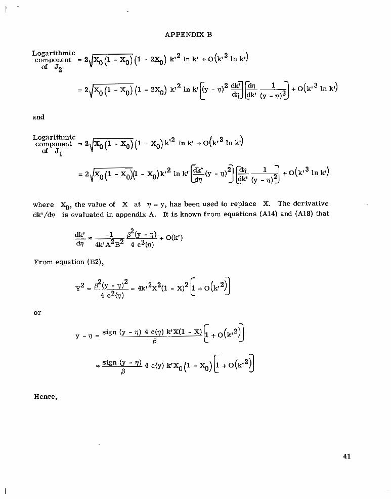
Logarithmic component = 2 , / x o o ( 1 - 2%) k t 2 In k' + O(kf3 In k')

of J2

1 - Xo) (1 - 2X0) k' I n k ' [(y -

q ) -- ,]..(kf31nk') dq dk' (Y - r l )*Jp

and

Logarithmic component = 2,/-( 1 - Xo) k t 2 In k' + O(kf3 In k') Of J1

+ O(kt3 Ink')

where %, the value of X at q = y, has been used to replace X. The derivative dk' /dq is evaluated in appendix A. It is known from equations (A14) and (A18) that

From equation (B2),

o r

- sign (y 4 c(y) k'Xo (1 - Xg) + 0(kt22]P

Hence,

41

APPENDIX B

2 -=drl - 4k'XZ (1 - xo) . . ..4 C2(Y) P + O(k') dk' 1

$4 c(y) k'% (1 - Xo) sign (y - q ) + O(kt2]

Furthermore,

drl 1 P2 dk' (Y - 17) - P-2= 16 c2(y) kv2X02(1 - Xo)

P= -sign (y - q ) 4 c(y) kT2X0(1- Xo)

It follows that

Logarithmiccomponent = ,#-(I - 2X0) k' 2 In k' (Y - ?)) P + O ( b 1 + O ( k t 3 In k')

(1 - Xo)of J2 4 c(y) kY2XO

Similarly,

42

APPENDIX B

Logarithmic dk'component = 2 (1 - Xo) dXo (1 - Xo) k' 2 In k' -(y - q ) B + O(kT3Ink') J1 dq 4 c(y) kV2XO(1 - Xo)1

= -sign (y - q ) 2 C(Y)

(y - q )2 dk' k' + O(kt3 In k')-In dv

If equations (B10)and (B11)are substituted into equation (14),the logarithmic com­ponent of I

j can be shown to be

J :[ %!-&L . = - g (@) + (1 - X)g2($Ig [sign (y - q ) C(Y) Sln $I

(y - q)2 In k' + O(kt3 In k'

+ (j + 1) sin (j + 1)a - j s in j$I + ( j + 1) sin (j + l)@ 1 + cos sin $I sin $I

(y - q)2 In k' = -sign (y - q ) ;P

C(Y)drl Gj($I)

where

It should be noted that equation (B12)can be reduced to the conventional form, such as that used by Wagner (ref. 5), by' simply using equation (B9)f o r dk'/dq:

43

APPENDIX B

= -sign (y - q) P c(y> sin24

and to the f i r s t approximation,

If only the t e rm associated with In IYI is retained, it is seen f rom equation (B12) that

where c(y) has been expressed in t e r m s of c(q) through the relation

Since

it follows that

44

I

APPENDIX B

which is the same expression as that used by Wagner (eq. (16b) of ref. 5) except f o r the factor 2/7r which is due to the different definition of hj (@l) used here in this report.

To perform the spanwise integration defined in equation (5), the chordwise influence function I.(X,Y,q) and the loading function q.(q) I.(X,Y,q) may be decomposed asJ J J follows:

When equations (B14) and (B15) are substituted into the spanwise integral in equation (5), the first t e rm in equation (B15) can be exactly integrated and gives

The notation has been made compatible with Multhopp's notation (ref. 1). Reference 7 gives a detailed explanation of the subscripts which have been introduced. It follows that

= -5' qj(yv)2n-c(yv) Gj

(GS)(k; In k; - k i + k i In kb - kb) j=O

45

APPENDIX B

where

A22 = (1 - x2)2 2 + y2

If c(-1) = c(1) = 0 (i.e., the taper ratio is zero), the limiting values for k i and k i must be used:

46

APPENDIX B

lim ki2 = lim 4 c2(-1) c (-1)-0 c( -1)-0

4

l imwhere d (y .> is the x-location of the midchord at y,. Similarly, c(+l)-0

ki2 = 1. It

follows that

for a symmetrical wing in which c(1) - 0 and c(-1) - 0.

The spanwise integration of the second and third t e rms in equation (B15) can be accomplished by Multhopp's method of integration. Substitution of equation (B12) for Ljresul ts in

Multhopp's method of integration can be applied by using the trigonometric interpolation formula of the type

47

- --

APPENDM B

a nawhere 8 n

= -2 m + l

and m is the number of spanwise integration stations over the

whole wing. Thus,

where the prime on the summation sign means that the t e r m with n = v is omitted from the summation and

B2 = X2 + Y2

kf 2 = (A + B)2 - 1 vn 4AB

~

Gj (@s) =

cos j6s + cos (j + 1) 6, cos 6, + j sin j$JS + ( j + 1) sin (j + 1) @s

sin @s

48

APPENDIX B

A1so

m + l 4 sin oV

(In - v ) odd)

I O V V = i r p s + sin +s)

Combination of equations (B16)and (B19)gives the total induced downwash:

49

APPENDIX C i

IMPROVEMENTS IN LANGLEY PROGRAM A0313

The improvement in the logarithmic-singularity correction t e rm presented in this report has been implemented into the analysis version of the computer program described in the supplement to reference 7 (Langley program A0313). In addition,

(1)The program has been restructured into an overlay arrangement (core require­ments of 510008 words on the Control Data 6600 computer system).

(2) The chordal loading functions of reference 5 a r e employed.

(3) The test to set the values f o r N and m is utilized before a solution is begun.

(4) Damping in roll, damping in pitch, and side-edge suction-force computations have been added. In order to access these items, the format of the third data input card has been changed to 5F6.0, F6.2, and 4F6.0 with the las t three fields set aside to receive the codes needed to commence these computations. The codes a r e as follows:

(a) In columns 43 to 48, a 1 causes the damping-in-roll stability derivative to be computed; a 0 indicates that C is not desired.

czP ZP (b) In columns 49 to 54, a 1 causes the damping-in-pitch stability derivative

C and the lift coefficient due to pitch rate C to be computed; a 0 indicates mqthat Cm and C a r e not required. Lq

q Lq (c) In columns 55 to 60, a 1 causes the side-edge suction force to be computed

and the aerodynamic characterist ics as a function of angle of attack to be listed; a 0 indicates that neither the side-edge suction force nor a listing of the aerodynamic characterist ics is required.

Note that roll-rate and pitch-rate stability derivatives cannot be computed simultaneously. Also, the side-edge suction force should not be computed concurrently with roll-rate or pitch-rate derivatives.

This version of the computer program is available f rom COSMIC, 112 Barrow Hall, University of Georgia, Athens, GA 30602.

50

REFERENCES

1. Multhopp, H.: Methods for Calculating the Lift Distribution of Wings (Subsonic Lifting-Surface Theory). R . & M. No. 2884, Brit ish A.R.C., Jan. 1950.

2. Zandbergen, P. J.; Labrujere, Th. E.; and Wouters, J. G.: A New Approach to the Numerical Solution of the Equation of Subsonic Lifting Surface Theory. NLR TR G.49, Natl. Aero-Astronaut. Res. Jnst. (Amsterdam), Nov. 1967.

3. Medan, Richard T.: Improvements to the Kernel Function Method of Steady, Sub­sonic Lifting Surface Theory. NASA TM X-62,327, 1974.

4. Rowe, W. S . ; Winther, B. A.; and Redman, M. C.: Prediction of Unsteady Aerody­namic Loadings Caused by Trailing Edge Control Surface Motions in Subsonic Compressible Flow - Analysis and Results. NASA CR-2003, 1972.

5. Wagner, Siegfried: On the Singularity Method of Subsonic Lifting-Surface Theory. J. Aircr., vol. 6, no. 6, Nov.-Dec. 1969, pp. 549-558.

6. Van de Vooren, A. I.: Some Modifications to the Lifting Surface Theory. J. Eng. Math., vol. 1, no. 2, Apr. 1967, pp. 87-102.

7. Lamar, John E.: A Modified Multhopp Approach f o r Predicting Lifting P res su res and Camber Shape for Composite Planforms in Subsonic Flow. NASA T N D-4427, 1968.

8. Jordan, Peter F.: Remarks on Applied Subsonic Lifting Surface Theory. Jahrb. 1967 WGLR, Hermann Blenk and Werner Schulz, eds., c.1968, pp. 192-210.

9. Mangler, K. W.; and Spencer, B. F. R.: Some Remarks on Multhopp's Subsonic Lifting-Surface Theory. R. & M. No. 2926, British A.R.C., 1956.

10. Wegener, F.: Zur Programmierung von Verfahren fu r die Berechnung der Auftriebsverteilung an Tragfliigeln. Jahrb. 1958 WGL, Hermann Blenk and Werner Schulz, eds., Fr iedr . Vieweg & Sohn, c.1959, pp. 48-53.

11. Byrd, Paul F.; and Friedman, Morr is D.: Handbook of Elliptic Integrals for Engineers and Scientists. Second Ed., Revised. Springer-Verlag, 1971.

51

I

L S cOLD NEW

N 0 2 e r­a4 m I

O h.,- +2.0

I----

CD, ii C 1.2

D, i

08

-6 11 16 21 26 31 36 41

m (a) Aspect-ratio-2 rectangular wing.

Figure.1.- Effect of LSC on near-field to far-field vortex drag ratio for two planforms at various values of N. M = 0.

L S c OLD NEW

N N 0 2 + 2 0 4 M 4 0 6 + 6

3

2

0

- 1 6 11 16 21 26 31 36 41

m (b) Aspect-ratio-4 delta wing; A = 45'.

Figure 1.- Concluded.

- - - - -

.. .. d

NATIONAL AERONAUTICS AND SPACE ADMINISTRATION WASHINGTON, D.C. 20546 POSTAGE A N D FEES P A I D

N A T I O N A L AERONAUTICS A N D SPACE A D M I N I S T R A T I O N !

OFFICIAL BUSINESS 481 PENALTY FOR P R I V A T E U S E $300 THIRD-CLASS BULK RATE U

5 1 IU,A, lUU!I/ S U U Y O S D SDEPT �ETHE A I B FORCE AF 3iBIPQIS Ld3OBATQRY ATTN : TECBIICAL LIBRARY (SU t ) KIRTLAID AFB HI! 87117

- - _--­ -

If Undeliverable (Section 168POSTMASTIR : Poxtnl Mnnunl) Do Not Return

‘The a T o m activities of the United States shall be conducted so 6 . . to the expansion of human knowl­edge of phenoj 5 , osphere and space. The Administration shall provide fo+ ,racticable and appropriate dissemination of information cone. It; activities and the results thereof.”

-NATIONAL AERONAUTICSAND SPACE ACT OF 1958

NASA SCIENTIFIC AND TECHNICAL PUBLICATIONS TECHNICAL REPORTS: Scientific and technical information considered important, complete, and a lasting contribution to existing knowledge.

TECHNICAL NOTES: Information less broad in sco,pe but nevertheless of importance as a contribution to existing knowledge.

TECHNICAL MEMORANDUMS:

Information receiving limited distributionbecause of preliminary data, security classifica­tion, or other reasons. Also includes conference proceedings with either limited or unlimited distribution.

CONTRACTOR REPORTS: Scientific and technical information generated under a NASA contract or grant and considered an important contribution to existing knowledge.

TECHNICAL TRANSLATIONS: Information published in a foreign language considered to merit NASA distribution in English.

SPECIAL PUBLICATIONS : Information derived from or of value to NASA activities. ‘Publications include final reports of major projects, monographs, data compilations, handbooks, sourcebooks, and special bibliographies.

TECHNOLOGY UTILIZATION PUBLICATIONS: Information on technology used by NASA that may be of particular interest in commercial and other-non-aerospace applications. Publications include Tech Briefs, Technology Utilization Reports and Technology Surveys.

Details on the availability of these publications may be obtained from:

SCIENTIFIC AND TECHNICAL INFORMATION OFFICE

N A T I O N A L A E R O N A U T I C S A N D SPACE A D M I N I S T R A T I O N Washington, D.C. 20546