nasa contractor report · foci of sound propagated in i00 successive pertrubations of the...

NASA

o_o'3

!

Z

CONTRACTOR

REPORT

NASA CR-1337

THE _'_'_° _ _r,rre_ i a OF ATIvIOSPHeRIC

FLUCTUATIONS AND REPRESENTATION

UPON PROPAGATED SOUND

by R. C. Bundgaard

Prepared by

KAMAN SCIENCES CORPORATION

Colorado Springs, Colo.

for George C. Marshall Space Flight Center

NATIONAL AERONAUTICS AND SPACE ADMINISTRATION • WASHINGTON, D. C. • APRIL 1969

https://ntrs.nasa.gov/search.jsp?R=19690013834 2020-04-08T06:59:34+00:00Z

NASA CR- 1337

THE EFFECTS OF ATMOSPHERIC FLUCTUATIONS AND REPRESENTATION

UPON PROPAGATED SOUND

By R. C. Bundgaard

Distribution of this report is provided in the interest of

information exchange. Responsibility for the contents

resides in the author or organization that prepared it.

Issued by Originator as Report No. KN-67-698-2

Prepared under Contract No. NAS 8-11348 by

KAMAN SCIENCES CORPORATION

Colorado Springs, Colo.

for George C. Marshall Space Flight Center

NATIONAL AERONAUTICS AND SPACE ADMINISTRATION

For sale by the Clearinghouse for Federal Scientific and Technical Information

SpringfleJd, Virginia 22151 - CFSTI price $3.00

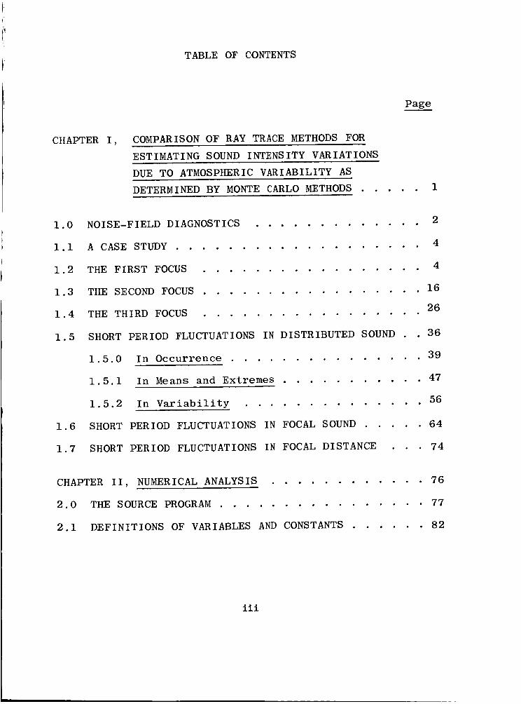
TABLE OF CONTENTS

Page

CHAPTER I, COMPARISON OF RAY TRACE METHODS FOR

ESTIMATING SOUND INTENSITY VARIATIONS

DUE TO ATMOSPHERIC VARIABILITY AS

DETERMINED BY MONTE CARLO METHODS ..... 1

1.0

I.I

1.2

1.3

1.4

1.5

2NOISE-FIELD DIAGNOSTICS .............

A CASE STUDY .................. 4

4THE FIRST FOCUS .................

THE SECOh_ FOCUS ................. 16

26THE THIRD FOCUS .................

SHORT PERIOD FLUCTUATIONS IN DISTRIBUTED SOUND 36

1.5.0 In Occurrence ............... 39

1.5.1 In Means and Extremes .......... 47

561.5.2 In Variability ..............

SHORT PERIOD FLUCTUATIONS IN FOCAL SOUND ..... 64

SHORT PERIOD FLUCTUATIONS IN FOCAL DISTANCE • 74

CHAPTER II, NUMERICAL ANALYSIS ............ 76

2.0 THE SOURCE PROGRAM ................ 77

2.1 DEFINITIONS OF VARIABLES AND CONSTANTS ...... 82

iii

2.2 PROGRAM ALLSOND

2.2.0

2.2.1

2.2.2

2.2.3

2.2.4

2.2.5

2.2.5

2.2.6

2.2.7

2.2.8

2.2.5

2.2.6

................. 130

Mainline ................. 130

Subroutine ADJUST ............. 144

Subroutine TENSITY ............ 145

Subroutine FIT .............. 149

Subroutine PRINT1 ............. 150



Subroutine FOCI SUM ............ 158

Subroutine FOCC SUM ............ 161

Subroutine PRINT4 ............ 164

INSYM .................. 165

SYMBOLIC INPUT ............... 167

CHAPTER III, NUMERICAL RESULTS ............ 171

3.0 TABLE V, FOR A SEOUENCE OF PERTURBATIONS OF THE

ATMOSPHERE REPRESENTED BY BOTH LINEAR

AND PARABOLIC LAYERS, THE DISTANCE TO

FOCAL POINTS AND VALUE OF SOUND INTEN-

SITY THERE ............... 172

3.1 TABLE VI, FOR A SEQUENCE OF PERTURBATIONS OF THE

ATMOSPHERE REPRESENTED BY BOTH LINEAR

AND PARABOLIC LAYERS, A COMPARISON OF

THE DIFFERENCES BETWEEN THESE REPRESENT-

ATIONS IN TERMS OF THEIR RESPECTIVE

IDENTIFICATION OF THE SAME FOCI .... 177

iv

3.2 TABLE VII, FOR A SEQUENCE OF PERTURBATIONS OF

THE ATMOSPHERE REPRESENTED BY BOTH

LINEAR AND PARABOLIC LAYERS, THE

DISTRIBUTION OF SOUND INTENSITY AT

XI ALONG 45 DEGREES AZIMUTH ON FEB

27, 1964, 1636CST ......... .182

3.3 TABLES VIII:

3.3.0 ABLE,

3.3.1 ABLE,

3.3.2 BRAVO,

3.3.3 BRAVO,

A DISTRIBUTION SUMMARY FOR MIN TYPE

FOCI OF SOUND PROPAGATED IN i00

SUCCESSIVE PERTURBATIONS OF THE

ATMOSPHERE REPRESENTED BY STRAIGHT-

STEPPED LAYERS.

A DISTRIBUTION SUMMARY FOR MAX TYPE

FOCI OF SOUND PROPAGATED IN I00

SUCCESSIVE PERTRUBATIONS OF THE


STEPPED LAYERS.

A DISTRIBUTION SUMMARY FOR MIN TYPE



ATMOSPHERE REPRESENTED BY PARABOLIC-

SMOOTH LAYERS.

A DISTRIBUTION SUMMARY FOR MAX TYPE

FOCI OF SOUND PROPAGATED IN I00



SMOOTH LAYERS ............ 185

V

CHAPTER IV, CONCLUSIONS ............... 189

REFERENCES .................... 194

vi

LIST OF ILLUSTRATIONS

Figure T I T LE Page

FREQUENCY DISTRIBUTION OF DISTANCE (r) TO

NEAREST SOUND FOCUS ..............

COMPARISON OF LINEAR AND PARABOLIC MODELS IN

TERMS OF THE IDENTIFICATION AND RANGING OF A

MINIMUM-TYPE FOCUS DURING SMALL-SCALE TIME-

VARIATIONS OF THE ATMOSPHERE ........ 5

3 COMPARISON OF LINEAR AND PARABOLIC MODELS IN

TERMS OF THE IDENTIFICATION AND INTENSITY

(DB) OF THE FOCUS CONSIDERED IN THE PREVIOUS

FIGURES .................. 7

4 IDENTIFICATION AND INITIAL INCLINATION OF

RAYS REACHING THE FOCUS CONSIDERED IN THE

PREVIOUS FIGURES ............... l0

5 STRENGTH AND LOCATION OF NEAREST SOUND FOCUS. . Ii

6 CHARACTER OF NEAREST SOUND FOCUS ....... 13

7 FREQUENCY DISTRIBUTION OF DISTANCE (r) TO

NEXT-NEAREST SOUND FOCUS ............ 15

vii

8 IDENTIFICATION AND INCLINATION OF RAYS

REACHINGTHE NEXT NEAREST, MINIMUM-TYPEFOCUS ..................... 17

9 IDENTIFICATION AND INTENSITY (DB) OF SECOND

NEAREST, MINIMUM-TYPE FOCUS .......... 18

I0 THE IDENTIFICATION AND RANGING OF THE NEXT

NEAREST, MINIMUM-TYPE FOCUS .......... 20

ii INTENSITY AND POSITION OF OTHER SOUND FOCI

WITHIN 40 KM OF SOURCE ............ 21

12 CHARACTER OF THE OTHER FOCI ......... 23

13 FREQUENCY DISTRIBUTION OF DISTANCE (r) TO THE

NEAREST AND NEXT-NEAREST MAXIMUM-TYPE FOCUS . 25

14 THE IDENTIFICATION AND RANGING OF THE NEXT-

NEAREST, MAXIMUM-TYPE FOCUS .......... 27

15 THE IDENTIFICATION AND INTENSITY OF THE NEXT-

NEAREST, MAXIMUM-TYPE FOCUS .......... 28

16 IDENTIFICATION AND INITIAL INCLINATION OF RAYS

REACHING THE NEXT-NEAREST, MAXIMUM-TYPE FOCUS . 31

17 LINEAR SOUND DISTRIBUTION FOR i00 SMALL-SCALE

AND RANDOM VARIATIONS OF THE ATMOSPHERE .... 37

viii

18 PARABOLIC SOUNDDISTRIBUTION FOR 100 SMALL-

SCALE VARIATIONS IN THE ATMOSPHERICSTATE . . . 45

19 RANGEDIFFERENCES IN INTENSITY BETWEEN LINEAR

AND PARABOLIC SOUND DISTRIBUTION OVER I00

SMALL-SCALE VARIATIONS IN THE ATMOSPHERIC

STATE ..................... 46

20 SOUND-INTENSITY DIFFERENCES BETWEEN LINEAR

AND PARABOLIC DISTRIBUTIONS OVER i00 SMALL-

SCALE VARIATIONS IN AN ATMOSPHERIC STATE .... 48

21

22

A DISTRIBUTION SUMMARY OF SOUND INTENSITY

FROM THE LINEAR REPRESENTATION OF PERTURBED

ATMOSPHERES ...............e. • •

49

A DISTRIBUTION SUMMARY OF SOUND INTENSITY

FROM THE PARABOLIC REPRESENTATION OF

PERTURBED ATMOSPHERES ............. 51

23 THE STANDARD DEVIATION IN THE LINEAR AND PARA-

BOLIC SOUND DISTRIBUTIONS OVER 100 SMALL-SCALE

PERTURBATIONS OF AN ATMOSPHERE ........ 57

24 VARIABILITY IN SOUND DISTRIBUTION COMPARED

BETWEEN THE TWO METHODS ............ 59

25 DIFFERENCES IN THE VARIABILITY OF SOUND

INTENSITY AND IN THE NUMBER OF RAY LANDINGS . . 60

ix

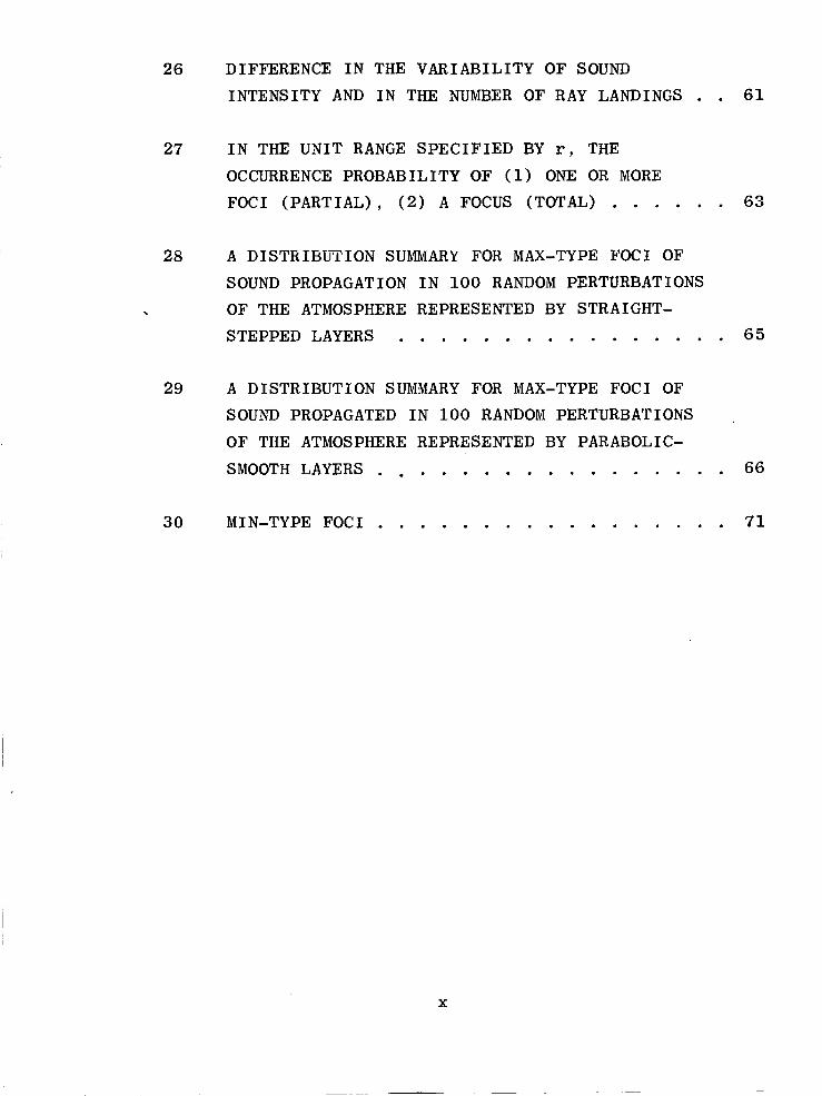
26 DIFFERENCE IN THE VARIABILITY OF SOUND

INTENSITY AND IN THE NUMBER OF RAY LANDINGS 61

27 IN THE UNIT RANGE SPECIFIED BY r, THE

OCCURRENCE PROBABILITY OF (I) ONE OR MORE

FOCI (PARTIAL), (2) A FOCUS (TOTAL) ...... 63

28 A DISTRIBUTION SUMMARY FOR MAX-TYPE FOCI OF

SOUND PROPAGATION IN I00 RANDOM PERTURBATIONS

OF THE ATMOSPHERE REPRESENTED BY STRAIGHT-

STEPPED LAYERS ................ 65

29 A DISTRIBUTION SUMMARY FOR MAX-TYPE FOCI OF

SOUND PROPAGATED IN i00 RANDOM PERTURBATIONS

OF THE ATMOSPHERE REPRESENTED BY PARABOLIC-

SMOOTH LAYERS ................. 66

30 MIN-TYPE FOCI ................ 71

X

LIST OF TABLES

Table T I TLE Page

I CLOSELY SPACED PAIRS OF MIN-TYPE,

CLOSE-IN FOCI IDENTIFIED BY THE

PARABOLIC MODEL ........ 8

II OCCASIONS WHEN X-NUMBER OF MAX-TYPE

FOCI WERE IDENTIFIED BY THE LINEAR-

LAYER MODEL AS COMPARED WITH Y-NUMBER

OF SUCH FOCI BEING FOUND BY THE PARA-

BOLIC MODEL ............... 3O

IIIA IN DB, THE RANGING OF FOCAL INTENSITY

OVER THE UNIT-KILOMETER RADIAL INTERVALS

IN EACH OF WHICH MAX-TYPE FOCI OCCURRED . • 68

IIIB IN DB, THE ALGEBRAIC DIFFERENCE IN THE

MEAN FOCAL INTENSITY PER UNIT-KILOMETER

INTERVAL, THE DIFFERENCE BEING TAKEN

FROM ONE INTERVAL TO THE NEXT OUT

INTERVAL ................. 69

IV COMPARISON OF FOCAL AND INTER-FOCAL

SOUND VARIABILITY ............. 70

V FOR A SEQUENCE OF PERTURBATIONS OF THE

ATMOSPHERE REPRESENTED BY BOTH LINEAR AND

PARABOLIC LAYERS, THE DISTANCE TO FOCAL

POINTS AND VALUE OF SOUND INTENSITY THERE . 172

xi

VI FOR A SEQUENCE OF PERTURBATIONS OF


LINEAR AND PARABOLIC LAYERS, A

COMPARISON OF THE DIFFERENCES BETWEEN

THESE REPRESENTATIONS IN TERMS OF

THEIR RESPECTIVE IDENTIFICATION OF

THE SAME FOCI ............... 177

VII FOR A SEQUENCE OF PERTURBATIONS OF


LINEAR AND PARABOLIC LAYERS, THE

DISTRIBUTION OF SOUND INTENSITY AT

XI ALONG 45 DEGREES AZIMUTH ON FEB.

27, 1964, 1636CST ............. 182

VI I I -ABLE A DISTRIBUTION SUMMARY FOR MIN TYPE




STEPPED LAYERS .............. 185

VI I I -ABLE A DISTRIBUTION SUMMARY FOR MAX TYPE




STEPPED LAYERS .......... 186

VI I I-BRAVO A DISTRIBUTION SUMMARY FOR MIN TYPE



xli


STEPPED LAYERS .............. 187

VIII-BRAVO A DISTRIBUTION SUMMARY FOR MAX TYPE

FOCI OF SOUND PROPAGATED IN 100



SMOOTH LAYERS .............. 188

xlii

SUMMARY

A solution is required to the general problem of

estimating expected variations in sound intensity level.

The sound originates from an intense noise source located

on the ground. The estimate is to be made at other points

on the ground. These points vary in distances from the

source. They may be within a few kilometers of the source

or several tens of kilometers away. The variations are due

to meteorological factors.

In this study, the diagnosed strength of noise fields

has been obtained by the conventional ray-tracing method.

When this method is applied to the general problem, the

procedure suffers from two disadvantages. First, the pro-

cedure does not always give an estimate. Second, in several

instances, its application may be physically unsound.

Wherever the ray method does give an estimate, however,

it has been found that the estimated field strength depends

upon a number of considerations. In part, its occurrence

depends on the observed atmosphere. The horizontal wind-

and sound-speed varies along the local vertical and with

time. Its variation is not fully described by the discrete

observations. Yet, it is known that this variation pro-

nounces big changes in noise fields.

In part, the noise field depends on the way in which

the observed atmosphere is to be represented. Atmospheric

changes are continuous in space and time. Meteorological

practice attempts to approximate the smoothly changing

atmosphere. The approximation is a straight-stepped repre-

sentation of aerological data at rather large time intervals

(6 to 12 hours). This instantaneous linear representation

is a convenient custom. It is quite easy to linearize the

xiv

variation of horizontal wind- and sound-speed along the

local vertical. Data points are connected with straight

lines.

But, it is suspect that such a linearized variation

introduces certain characteristics in the outward rang-

ing of sound and its intensity. These features are not

real. They are unwanted. In this study, an attempt is

made to apprehend them, to find out when they happen,

how often they take place, how big they are, to see how

much they vitiate or change the real noise field.

Due to representation, the change in the true noise

field may look like that due to the unobserved variations

in the atmosphere. In the effort of this study, it is

desirable to distinguish one such change from the other.

The distinction is necessary for pin-pointing the noise

field changes that result from the straight-stepped

representation of aerological data.

Among others, two special techniques are employed in

order to effect this distinction between the noise-field

change due to representation and that due to the unobserved

variations. One makes up for the inadequacies in observa-

tion. The other, for the short-comings in representation.

A numerical technique is used for estimating short-

period fluctuations in the noise fields, by means of an

artificial experiment for sampling small-scale changes in

the atmosphere -- the Monte Carlo method. The resulting

estimate yields information as to the occurrence of small-

scale time-induced change in the noise fields, and infor-

mation as to its likelihood, average value and variability.

A non-linear technique is introduced for representing

X-V

the aerological observations. It violates none of the

assumptions on which the ray-tracing methods are based.

The representation is easily obtained. It is descrip-

tive of the real atmosphere.

This report compares the two methods for estimat-

ing sound intensity and compares the results obtained

by them. It concludes that the linear method introduces

big errors into the diagnosed strength of noise fields.

It recommends that non-linear methods be used instead of

the straight-stepped representation of aerological para-

meters.

xvi

CHAPTER I

COMPARISON OF RAY TRACE METHODS

FOR ESTIMATING SOUND INTENSITY VARIATIONS

DUE TO ATMOSPHERIC VARIABILITY AS DETERMINED

BY MONTE CARLO METHODS

- 2 -

1.0 NOISE-FIELD DIAGNOSTICS, A CASE STUDY

The static firings of rocket engines generate noise

fields. These fields vary according to the atmospheric

conditions. In addition, these fields are affected just by

the way in which the atmospheric conditions are to be rep-

resented. Along the local vertical a straight-stepped repre-

sentation of the meteorological parameters has been a custo-

mary approximation to the smoothly changing atmosphere. But

a non-linear representation is also available.

These representations lead to two methods for diagnosing

noise fields generated by static test-firings of large boosters.

Previous studies have examined each method. Based upon their

findings, the study reported here applies the two methods and

compares the results obtained by them.

In this chapter, the comparison is carried out through a

case study made of the two methods (Section I.i). This case

involves three sound foci, offering interesting situations for

comparing the two methods (Sections 1.2, 1.3 and 1.4). Around

these loci, the noise field varies with the short-period fluc-

tuations that occur in the atmosphere (1.5). Between loci,

the ray-method may lead incorrectly (or incompletely) to sound

shadow-zones, which vary with atmospheric fluctuations. The

likelihood itself varies as to whether or not sound occurs at

all (1.5.1). Big changes may occur in the inter-focal dis-

tribution of the sound propagated in a turbulent atmospheric

continuum. Because of fluctuations in the propagating medium,

the mean intensity of the distributed sound varies within

changing extremes (1.5.2). Generally, the distributed sound

shows considerable variation with the small-scale alterations

in the atmospheric conditions (1.5.3). Finally, this chapter

closes with the important findings as to the short-period

fluctuations in the focal sound itself (1.6), and in focal

distance (1.7).

-3-

i

\

F.._ Lm

- 4 -

I.i A CASE STUDY

A case-study approach is made for the comparison of the

two methods for estimating sound intensity. The case now

considered is the one for February 27, 1964, 16:36 CST, at

Huntsville, Alabama. This situation is chosen to introduce

the comparison, because of simplicity of the sound distribution.

The atmospheric sounding of sound-propagation speed has two,

pronounced inversions (graphic representation of this sounding

may be found in Fig. 2a, p. 153 of KN-66-698-1(F)). The lower

one, which occupies the 400-900 meter layer, yields a single

but pronounced sound focus about eight kilometers out from the

source along the chosen azimuth of 45 ° The upper inversion

pronounced and extensive above 2,500 meters, produces two well-

defined loci about 30- to 35 km out. One of these is a minimum

type focus.

These three foci remain identifiable during small-scale

time variations (fractions of an hour) of this initial atmos-

pheric state. Yet, in their range and intensity, they offer

variations sufficient to test the two methods over a wide

variety of conditions• During these variations, a fourth and

maximum-type focus sometimes returns close-in. Most other

cases offer complexing effects, especially in the linear-layer

methods, as well and up to a dozen foci or so, in the first

40-km range.

The discussion now proceeds to consider the three main

foci, beginning with the min-type closest in to the source.

1.2 THE FIRST FOCUS

Fig. 1 shows that, as determined by either method, the

nearest sound focus is confined to a relatively narrow 1.5

km. band, centered eight kilometers out. With small-scale

time-variations in the initial atmospheric state, this focus

- 5 -

8.5

8.4

8.3

8.2

8.1

_ 8.o-

I 7.9-

_ 7.8-

0

0m 7.7-<n,

n7.6

7.5

7.4

7.3

7.2

FOCI UNIDENTIFIED BY LINEAR MODEL,

-_1 FIGURE 2

COMPARISON OF LINEAR AND PARABOLIC MODELS IN TERMS OFTHE IDENTIFICATION AND RANGING OF A MINIMUM--TYPE FOCUSDURING SMALL--SCALE TIME--VARIATIONS OF THE ATMOSPHERE.

--1 SEE FIG. 1 FOR THE DEFINITION OF TERMS ANDCONDITIONS, WHICH ALSO APPLY TO THIS FIGURE.

1 / ///®

t ,,," oo-! /7 /, ok/ 16 o

--_ '. /_/ ///o ® o ®® o_. o_/ ,," o,, o-5 oO._ ,,"c _ ; g __./- _ // _/0.63 KM - /=; ,-:o oo o: ?./=5 / ,,/ o® o _ o./

®" /

//

®

0

O

//

//®

/ ®

®

--42222

_4_3"-'3

_3I

I--2

® /

0.4 KM®

®

oo //

//

m

I

7.6

®//

o ®/® FREQUENCY OF OCCURRENCE EVERY 250 METERS BY LINEAR METHOD

I II 1 22 3111 13424531244335312 25111 I

I I I I I I I I I 1

7.8 8.0 8.2 8.4 8.6LINEAR MODEL FOCAL DISTANCE (KM)

- 6 -

recurs within that narrow variation of radial range, whether

ascertained by the linear model or the parabolic-smooth model.

It recurs between the two with nearly equal persistency. The

basic impression gained from Fig. 1 would seem to be that the

two methods correspond well in the determination of the same

focus.

But, the area within the dashed bars is about 30% less

than that of the solid bars. For some reason, therefore, it

may be suspect that the linear model does sometimes fail to

identify even the close-in focus. The figure suggests, more-

over, that the linear-layer method shifts the focus about a

half kilometer farther out than the median position of that

focus according to the parabolic model.

In Fig. i; the solid bars display the column of numbers

along the left vertical in Fig. 2; whereas, the dashed bars of

Fig. 1 have been graphed from the row of numbers along the lower

part of Fig. 2. The discussion shall therefore now proceed to

compare the two methods in terms of the case by perturbed case

indentification of the nearest focus.

Fig. 2 shows the scattering of focal distances between

the two methods.

According to the experience simulated by the Monte Carlo

process, the focal ranging over very short periods (fractions

of an hour) does tend to vary in the same way whether determined

by the linear or the parabolic method. That is, in Fig. 2 the

points do distribute themselves somewhat closely along a straight

line with a slope of one.

Nonetheless, the distribution envelopes a strip about 0.4

km. wide. This possible uncertainty is about one-third of the

limit through which the focus did range over short periods.

Namely, the focus ranged from about 7.2 to 8.6 kin. out, with a

115

- ? .

11L

In

113-

N

112-

_ 111-

n.

110-

?FIGURE 3

COMPARISON OF LINEAR AND PARABOLIC MODELSIN TERMS OF THE IDENTIFICATION AND INTENSITY

(DB) OF THE FOCUS CONSIDERED IN THE PREVIOUSFIGURES. SOURCE--STRENGTH TAKEN AS 204 DB.

FOR FURTHER DETAILS, SEE FIG 1

I o /I o / /

II /o _ ////I

j o /

I o_ t ///

/ o ,,"® o / oo/

/ o °°Z°° /

109116

UNIDENTIFIED BY LINEAR MODEL'_I I I II I I i I I I

117 118 119LINEAR MODELIS FOCAL INTENSITY (DB)

LEFTWARD EXTENSION OF ABSCISSA:UNIDENTIFIED BY LINEAR MODEL (CONTD.)

I I I III I Ill I I I II HI II I I II I I I I I I ,

112 113 114 115 DB

8 m

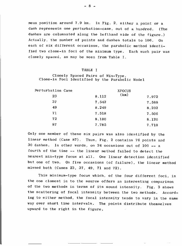
mean position around 7.9 kin. In Fig. 2, either a point or a

dash represents one perturbation-case, out of a hundred. (The

dashes are columnated along the lefthand side of the figure.)

Actually, the number of points and dashes totals to 106. On

each of six different occasions, the parabolic method identi-

fied two close-in foci of the minimum type. Each such pair was

closely spaced, as may be seen from Table I.

TABLE I

Closely Spaced Pairs of Min-Type,Close-in Foci Identified by the Parabolic Model

Perturbation Case XFOCUS

23 8.112 (km) 7.972

37 7.542 7.588

49 8.249 8.202

71 7.518 7.506

72 8.180 8.120

87 7.785 7.710

Only one member of these six pairs was also identified by the

linear method (Case 87). Thus, Fig. 2 contains 76 points and

30 dashes. In other words, on 24 occasions out of i00 -- a

fourth of the time -- the linear method failed to detect the

nearest min-type focus at all. One linear detection identified

but one of two. On five occasions (of failure), the linear method

missed both (Cases 23, 37, 49, 71 and 72).

This minimum-type focus which, of the four different foci, is

the one closest in to the source offers an interesting comparison

of the two methods in terms of its sound intensity. Fig. 3 shows

the scattering of focal intensity between the two methods. Accord-

ing to either method, the focal intensity tends to vary in the same

way over short time intervals. The points distribute themselves

upward to the right in the figure.

- 9 -

The median of this distribution, however, curves upward.The parabolic method tends to assign to a strengthening focusa greater increase in intensity than does the linear method,

although in an absolute sense the parabolic method comes upwith somewhat weaker sound foci than does the linear method

-- the difference being about 6 DB. (cf. columns 9 - ll,Table VI, p.182). With strengthening focal intensity, thedifference increases markedly in the intensity estimated bythe two methods. As seen in Fig. 3, the distribution of

the points fans outward and upward.

From considerations having been made elsewhere, it isknown that the parabolic method violates none of the assump-

tions involved in the ray-tracing technique, whereas the

linear method does. For the moment at least, the following

presumption can therefore be offered. Case by perturbed-

case, the min-type focus closest-in that it is identified by

the parabolic method but not detected by the linear method

is a real focus. In the Monte Carlo sampling for variations

in sound propagation due to short period fluctuations in the

atmosphere, the intensities of such unmatched foci can be

presumed to be that given by the parabolic method. In Fig. 3,

the intensity of 30 such foci have been spotted by the row of

vertical dashes along the abscissa (and including those of the

foci connected by the vertical line at the upper right in the

figure; v. seq.)

These dashes fall into two groupings, which are confined

to those min-type foci closest-in of extreme intensities. A

small group includes those foci which are comparatively

intense. The large grouping includes those which are unusually

weak. The linear method fails to identify the foci of either

such group, according to the results shown in Fig. 3.

The two points connected by the vertical line, incidentally,

- 10 -

.5 4

i3.ob,lQ

Z2I-

Z_1Uz

I>.<¢ 12.0

J

<_I-Z,

aO

U

J0 11.0ID<

.3

10.0

PERTURBATION NUMBER ( TABLE V )

--37

UNIDENTIFIED BY LINEAR MODEL

--71

--47

-- 83--32

-il

m86

o

QCo

o o _® ® @

®@

G

G

®

®

o

®

67m4)--77-- 98

G

® ®

_o6)

®

®

G ®®

® ® ®

®

O

®®

®

@@

o%

® ®

®

®

®

®

_8--82-- 7_--66_78

--_. 7t34

--49

i i i i i ! i i i i i i 1 i i i i | i [ i i i | iI i I I

1.0 .5 12.0 .5 13.0 "

LINEAR MODEL'S INITIAL RAY--INCLINATION (DEG.)

FIGURE 4

IDENTIFICATION AND INITIAL INCLINATION OF RAYS REACHING THE FOCUSCONSIDERED IN THE PREVIOUS FIGURES. (FOR DETAILS AND DEFINITIONS,SEE FIGURE I).

- i1 -

130DB

128

126

124

122

120

118'

116

114

112'

110

7.!

- 130.713 DB

- 120.392 DB

8.017

I! I

8.0

L

MIN_o = 12. 605°

P

12"252°= <PoMIN.

IIIII

4I

IItI

IIIIIIII

8.258I

' 8'2. ' '8.4

II

\

\

PARABOLIC

: i8 6 _) 8.8

- 12 -

represent perturbation Case 87, which was discussed in

connection with Fig. 2 and Table I.

Physical considerations suggest that a useful way for

comparing the two methods lies in the behavior of the sound

ray directly reaching the focus. Between the two methods

applied together in 100 trials, accordingly, Fig. 4 shows

the scattering of the initial inclination of the ray reach-

ing the focus. Ray covariation (Fig. 4) exhibits greater

variability than either focal ranging (Fig. 2) or focal

intensity (Fig. 3).

Now, certain physical conditions underlie and therefore

restrict the application of ray-tracing concepts for eval-

uating sound intensity. As just stated, the parabolic method

violates none of these physical conditions, while the linear

method does. One may therefore assume that the focal identi-

fication and evaluation by the parabolic method are valid and

reliable. Then, the occasions without co-identification by the

two methods and the variations in values obtained by them might

be considered as evidence as to inadequacies and inaccuracies

in the linear method. As a didactic consideration, it suggests

next that the two methods be compared in terms of the sound

distribution in the vicinity of the focus examined in the

previous figures.

For the basic, unperturbed atmosphere, Fig. 5 compares

the two methods in terms of the sound distribution in the 8-9

km. radial interval along the 45 ° azimuth, in which this focus

occurs. The linear focus L occurs 8.258-km. out with an eval-

uated intensity of at least 130.713 DB. The ray landing directly

there is the one having the initial inclination at the source

of 12.252 °. The parabolic focus P of at least 120.392 DB is at

8.017 km., the direct landing point of the ray having an ini-

tial inclination of 12.605 °. Along each, the ray landings

range inward to these points and then back out again. Just

how this occurs is shown in Fig. 6.

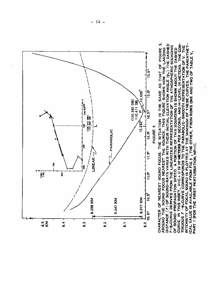
Fig. 6 compares the two methods in terms of certain

- 13 -

- 14 -

characteristics of the particular focus considered thus far.

This figure shows how the direct landing distance (r) of sound-

rays varies with their initial inclination angle (_o). The

abscissa looks at the 10-14 ° angular spread of a vertical fan of

rays leaving the sound source. These rays first land along a

half-kilometer interval starting about eight kilometers out

(the ordinate). As the ray paths elevate, their foot-prints

move first in toward the origin, then out again. This ray

behavior is detected by both methods. According to the linear

method, the foot-prints approach within 8.258 km., of the origin,

while they get 0.241 km. closer according to the parabolic method.

The minima L and P identify the focal positions of the previous

figure and the rays reaching them. The L and P are therefore

described as minimum-type foci.

In Fig. 6, two values of the focal sound intensity are

plotted at L and P. The one in parenthesis is the value ob-

tained from Fig. 5; the other includes the effect of wave

interference taking place at the focus. This value is obtained

from the Brekhovskikh equation (1) The Brekhovskikh value is

reported in Table V of this report (Part i; under the column

headed "TINF", see row "IABLE" for the L-value and row "IBRAVO"

for the P-value).

The diagram inset into Fig. 6 presents a portion of the

straight-stepped representation of the atmospheric sounding of

sound-propagation speed. As indicated by the vertical dashed

line, the ray landing at the focus L tops out at 700-meters

altitude (rows 12-13, column 8, Table IV-ABLE, p. 147,

KN-67-698-1).

In Fig. 6, the two r-_ ° curves differ appreciably in their

curvature at the focal position. The linear (dashed) curve

presents a shallow and flat trough; the parabolic one, a deep

and strongly curved trough. This focal curvature relates

directly to the focal intensity of sound; the greater the

- 15-

i,,-a

IF-II

29.5

\

--1 IILJ

LINEAR

(7"= 0.1M0 KM

m

F----I

.LL_I

J'IIIkn

II

3¢.5 32'.5I

30.5

r

10

iF1IIII

33!5MIN--TYPE FOCAL DISTANCE (KM)

II

I34.5

=,R,

FIGURE 7

FREQUENCY DISTRIBUTION OF DISTANCE (r)TO NEXT--NEAREST SOUND FOCUS.

THE CIRCUMSTANCES ARE THE SAME AS THOSE IN FIGURE 1.

- 16 -

curvature the weaker the sound. At the focal positions, this

difference in the shape of the two r-_o curves relates to the

difference in the peaking of the corresponding curves in Fig. 5.

Returning rays are "bounced"off straight-stepped inversions

in the atmospheric sounding of propagation speed, according to

the linearized treatment of sound propagation; whereas the non-

linear method returns them from continuously curved inversions.

In Fig. 6, the 9.942-14.274 ° fan of rays is all returned from

within the atmospheric layer AB, through which the linear method

represents the increase in propagation speed as being uniformly

linear. For that reason, the linear r-nPo curve is a trough

shallow in comparison with the parabolic one.

The sound distribution described in Figures 5 and 6 rep-

resents but one atmospheric situation out of the 100 summarized

in Figures 1 - 4; viz., the point C in Figures 2 - 4. This

situation is listed as Perturbation-Case 1 in Table V of this

report. Instead of considering some of the other 99 situations,

which will result in sound distributions different than shown

in Figures 5 and 6, the discussion will now turn to a similar

consideration of a second focus, the next nearest, minimum-

type focus that shows up rather regularly in the i00 trials

used in these discussions.

1.3 THE SECOND FOCUS

Fig. 7 shows how often this focus recurs over the 30-35 km.

range out from the source. The solid bars represent the column

of numbers along the left vertical in Fig. I0, while the dashed

bars of Fig. 7 have been graphed from the row of numbers along

the lower part of that figure. Compared to Fig. i, the fre-

quency distribution of Fig. 7 is broader and more flat. As in

the case of the focus closest in, the linear method places the

median position of the next nearest focus farther out than does

the parabolic method; the offset is about 0.4 km. For the

- 17 -

22.5

_-" 22,0

LdQ

<E 21.5-Z"-iI.)ZT>.<En, 21.0--I<E

m

ZN

.I 20.5-

0

U

0 20.0-I11

0.

19.5-

19.0

IZ.<I,IZ.3>.m

aIdhF-

.Jz

(1

m

Il

mm

mm

m

Imm

m

mm

i

m

m

.e

• • *C •

I 1 I I I

21.0 21.5 22.0 22.5 23.0

INITIAL RAY--INCLINATION (DEG)BY LINEAR MODEL

23.5

FIGURE 8

IDENTIFICATION AND INCLINATION OF RAYS REACHING THE NEXT NEAREST,MINIMUM--TYPE FOCUS.(THE CIRCUMSTANCES SET FORTH IN FIGURE 1APPLY ALSO TO THIS FIGURE. )

- 18- n,-,O,u,-,

i • r,.)..

_JI,d •a0

<ILlZ-1>.m

QbJb.

Z

_ •

,IIII IIInllllllI

tOC)

'0

-0

-0

m

N

-o_

Z

Z

h

-.jLda

5m_'_

blZN

_',_ro'_

-o_

o_

0

I

t t_ ® ,..

S ,-i':laOl_i Ol-IOeY_lVd

8h

hi

_aZ

;<

hi

Zb.

an,uZb.I

m OU_U

vD_Ul

I-

b.i-I1_

QZ<

mI-<UNhF-ZbJr_m

- 19 -

maximum frequency of occurrence per the same unit range, the

next nearest focus occurs half as often as does the nearest

focus. Short-time fluctuations in the focal distance have

increased with the increased range of the focus. (cf. Section

1.7,' p. 74)

In Fig. 7 the positional variability of the next nearest

focus is somewhat greater according to the linear method than

it is according to the parabolic method. The area under the

linear bar-graph is less than that of the parabolic bar-graph;

moreover, this aerial difference is greater than in Fig. i.

For the next-nearest focus, the number of misses by the linear

method is 47 compared to 30 for the focus nearest in.

During short period fluct_ons in the atmosphere, Fig. 8

shows that the initial inclination of the ray directly reach-

this next nearest focus varies from around 21-to about 23.5 ° .

This portion of the ray-fan tops out on a second, higher in-

version in the sounding of propagation-speed, at 4.5- to 5 Km.

Fig. 8 displays considerable scatter, as well as a large

number of occasions (47) in which the linear method failed in

detecting this focus.

For this next nearest focus, the assessed strength of

focal sound shows no evident relationship between the two

methods, according to the distribution of points in Fig. 9.

This is in contrast to relationship shown in Fig. 3 for the

closest in focus. In a great number of trials, moreover,

the linear method failed even to identify this next-nearest

focus (column of 47 dashes along ordinate). But, the most

significant feature of Fig. 9 is that, overall, the temporal

range of the focal strength is just 4.5 DB by the parabolic

method while it was 17.5 DB by the linear method; i.e.,

Fig. 9 is wide and flat. This four-fold difference suggests

that the character of the second nearest, so-called minimum

- 20 -

>-I--I

::)

m

Z

u-:u.n

n,nZ

×o w'-"

•- Z Ww n,

OLdW W

0 Zm

Z-I

ul Q_I-)-

'5 °wz o

bl

bl --I-

U__. --

ZW Ul

Z blU,,, z_0 I-

I

,CI_Q

2$

QO

_°°

II I II llllllgl IIIIIIIIIIIIIII 1 Ill II

m

qP,dl

m

P_

r',dl

O_

"ql"

e_

m

N

W

.J

00

n,

hlZ

3

7°

! I ! I I I I

(N_I) NONY.I.SIO 7_0_-I 7":lOON OlT08Y_IYd

- 21 -

0 U_

= o_8c.Z_

_8 _W

o0_z

Zz

o

¢41m

_I

g_

% o

Z

Jf ,__.o

n

0

\\\

I

III

I

I

/,

)II1 II1 "- _0 0 II _ -I

i _ ,,,,,,,,,,,,,,,,,,,__

CO Q

eq

u

- 22 -

type focus changes from case to perturbed case, as detected

by the linear method.

In a comparison of the closest and next closest loci,

Fig. 10 is a companion to Fig. 2. From the first to the

second focus, the increased scattering in the focal distance

as determined case-by-case by the two methods is very evident.

The striking difference in the character of the two sets

of figures; viz., Figures 7 - l0 and Figures 1 - 6; suggests

that the next nearest focus is somehow different than the

nearest one, even though both are minimum-type loci. The

discussion therefore turns to an examination as to the char-

acter of the next nearest focus.

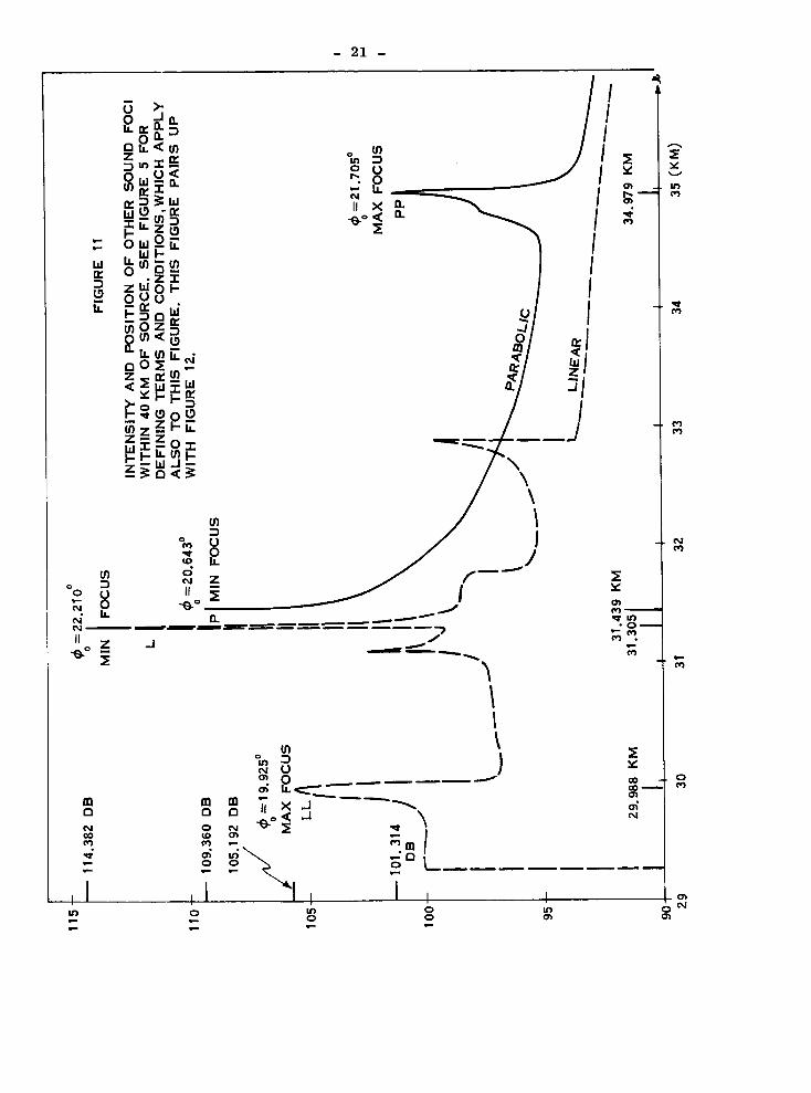
For the basic, unperturbed state of the atmosphere, the

sound distribution around this next nearest focus is shown in

Fig. 11. The spike L is the next nearest min-type focus accord-

ing to the linear method; whereas, P is the next nearest focus

according to the parabolic method. The L occurs 31.305 km. out

with an evaluated strength of at least 114.382 DB. Located

31.439 km. from the source, P has a focal intensity of at least

109.360 DB. The ray landing at L left the source at 22.210 °

elevation, while the one landing at P started with an initial

inclination of 20.643 ° . Both L and P are minimum type loci,

as can be seen from Fig. 12.

Determined by the two different methods, these same type

loci L and P are but 134 meters apart, some 30 kilometers away

from the source (Fig. 12). From these facts, one would conclude

that L and P are apprehending the same real focus, that their

measured differences in inclination, location and intensity are

a valid confirmation as to the validity of the two methods for

each estimating focal sound intensity. The L-P comparisons

summarized represents but one atmospheric situation of the 100

comparisons summarized in Figures 8 - 10; viz., the point C in

- 23 -

- 24 -

Figures 8 - i0. This situation is listed as perturbation-

case 1 in Table V of this report. The question arises,

why - overall - are these i00 comparisons so erratic, when

the analysis just made of perturbation - case 1 reveals a

comparison which is apparently good? To answer this ques-

tion, the discussion returns to a consideration of Figure

12.

This figure reveals some interesting properties about

the next nearest focus, as determined by the linear and

parabolic methods. Figure 12 will be examined in some

detail.

The parabolic r-_o curve (which is represented by the

heavy, unbroken line in the upper part of Figure 12) is

smooth; whereas the linear one (dashed) is discontinuous

in its derivative dr/d_o. The discontinuities M, R, S,

and T correspond to the data points M', R', S' and T' in

the linear representation of the atmospheric sounding of

propagation speed. Two portions of this sounding are

shown as insets in Figure 12. (Their details are the same

as those already set forth in the discussion of Figure 6.)

Consider the focus L, and its ray-ranging features,

which appear in the righthand part of Figure 12. From this

dashed, r-_o curve, it can be seen that L is a minimum-type

focus. The ray landing at L tops out at level L', which is

4544 meters high. This level is about midway between data

points S' and T'. As indicated parenthetically by minus

signs, negative discontinuities occur in the sounding lapse-

rate at data points S' and T' At these corresponding points

S and T in the dashed r(_o)-Curve , there is a negative dis-

continuity in dr/d_o ; i.e., with increasing initial-inclination,

the slope changes from positive values to negative values.

Ray zeniths are plotted at these break-points in the r(_o)-

curve (4471 meters at S and 4606 meters at T); these zeniths

- 25 -

Jr-

I I

o •Z II

"ib

vv

W

uz

a

>-!--I

x<

x<

Ul!--I-

w

IQ

wmZ_

z>

mWW

blUlU_z,,_

I-__.__.

,,z<_

w

zF-mbl --

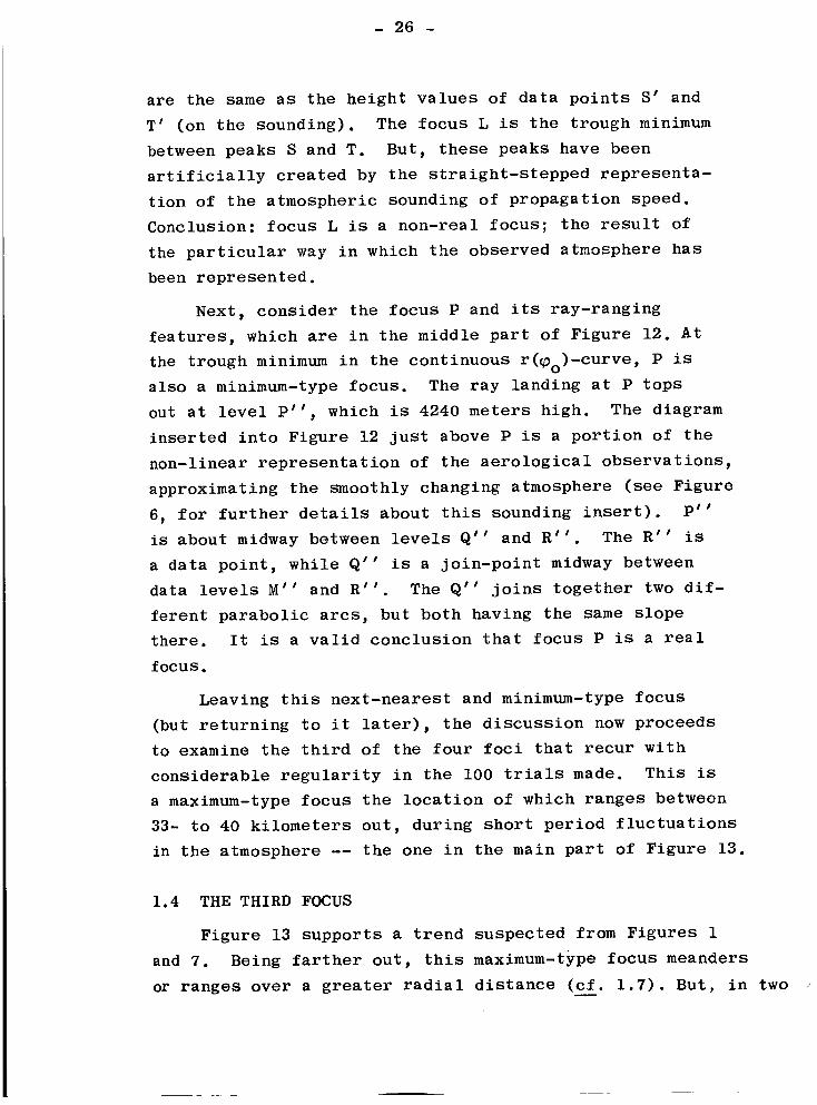
- 26 -

are the same as the height values of data points S' and

T' (on the sounding). The focus L is the trough minimum

between peaks S and T. But, these peaks have been

artificially created by the straight-stepped representa-

tion of the atmospheric sounding of propagation speed.

Conclusion: focus L is a non-real focus; the result of

the particular way in which the observed atmosphere has

been represented.

Next, consider the focus P and its ray-ranging

features, which are in the middle part of Figure 12. At

the trough minimum in the continuous r(_o)-Curve , P is

also a minimum-type focus. The ray landing at P tops

out at level P'', which is 4240 meters high. The diagram

inserted into Figure 12 just above P is a portion of the

non-linear representation of the aerological observations,

approximating the smoothly changing atmosphere (see Figure

6, for further details about this sounding insert). P''

is about midway between levels Q" and R''. The R'' is

a data point, while Q'' is a join-point midway between

data levels M'' and R''. The Q" joins together two dif-

ferent parabolic arcs, but both having the same slope

there. It is a valid conclusion that focus P is a real

focus.

Leaving this next-nearest and minimum-type focus

(but returning to it later), the discussion now proceeds

to examine the third of the four loci that recur with

considerable regularity in the I00 trials made. This is

a maximum-type focus the location of which ranges between

33- to 40 kilometers out, during short period fluctuations

in the atmosphere -- the one in the main part of Figure 13.

1.4 THE THIRD FOCUS

Figure 13 supports a trend suspected from Figures 1

and 7. Being farther out, this maximum-type focus meanders

or ranges over a greater radial distance (cf. 1.7). But, in two

- 2'7 -

O

oO

Ld• _ (.)

I-

D

'It

oe"

• .-i.I.urn"

• ?_--m--

"1":1aOI/! _I¥_INI-I Ag a'=ll--IIJ.N'=lalNn

I I I II I I III

I I I I I I I

m

Qhl

Zbl

Q

Z

(INN) ":IONV.LSIQ -IV::X).-I -13QOIN 1_llOlgVt:lVd

O0N

_0N

N

u;U0h

I--I

I,I

UlZI

- ×bl hn

0

1.9Z

Z,_ •

Z_

0--W

U m

I'-

Ul

- 28 -• trJ

• C)

• e °

II I IllU I I I I I

00

IJ')

mQ

v

>-I-

LdI-Z

.J

.<U

_m21Ul

0

iv,bl

I

WZ

.J

0r_

_D

Ill

h

tn

U0U.

WO..>I'-

I

,<

Ul

bJOzzI'<

Ulmzul

IM

b.

u_>-mI-

z-

I-I-zw-o

z

I-

uN

Is.

I-ZI.d0

I.d"1"I-

- 29 -

other respects, Fig. 13 is different from both Figs. 1

and 7. First, the maximum recurrence-frequency per unit

distance is greater by the linear method than the parabolic

method. Second, the median focal distance by the linear

method is less than by the parabolic method. Apparently,

something new characterizes this focus from the other two.

The scattering of focal distance is shown in Figure 14.

(The solid bars in Figure 13 have been plotted from the

column of numbers at the left in Fig. 14; the dashed bars,

from the row at the bottom.) The scattering is not as

buck-shot as Fig. i0, nor as patterned as Fig. 2. But,

the scattering does seem to fall somewhat along a vertical.

Focal ranging due to short-period fluctuations in the atmesphere

seem to be followed better by the parabolic method than

the linear one.

Fig. 14 differs also from Figs. 2 and I0 in the in-

creased number of multiple max-type loci identified case-

by-case by the linear method to every one by the parabolic

method; Figure 14 has 22 horizontal couplets; while Figure i0

has three, and Figure 2, none. Finally, Fig. 14 indicates

fewer loci unidentified by the linear-layer method than

Figs. 2 and I0.

In the scattering of focal intensity, Figure 15, similar

trends appear. The points tend to align vertically, etc.

The linear-layer method does not account for the variability

in focal intensity due to short-period fluctions in the

atmosphere; it also tends to introduce "spurious" maximum-

type loci from time to time, some of which have appreciably

different intensities than those found by the parabolic

method.

As identified by their initial elevation, the rays

reaching the maximum-type focus scatter according to the

two methods -- Figure 16. Certain details of this figure

- 30 -

merit special note. On 22 occasions, two linear loci

were identified for the one parabolic focus perturbed

(Case A, Table If). Six times, three linear loci occurred

TABLE I I

OCCASIONS WHEN X-NUMBER

OF MAX-TYPE FOCI WERE

IDENTIFIED BY THE LINEAR-

LAYER MODEL AS COMPARED

WITH Y-NUMBER OF SUCH

FOCI BEING FOUND BY THE

PARABOLIC MODEL

CA SE X Y FREQ.

A 2 1 22

B 3 1 6

C 4 1 1

D 1 2 1

E 2 2 5

F 3 2 1

Z X = 137

Z Y = 103

for the one parabolic focus found (Case B). And on one

occasion_ four linear loci were detected corresponding to

the one parabolic focus (Case C). These 29 cases are

represented in Fig. 16 by dots having flags flying to the

right; the left-most of the two or more linear foci for

¢,qN

N ll_

_.. ,--

•.":'._. I ...

°° oo •• o

i"II .,-

l.i .- ,,

-- N

Iwlg • t_.

N. .

w_m

II=;

I

II

•_® .JbJ

.9 00

Un0

O4

ii .f'13aol__ _IV':INI"I A9 a':ll.-iiJ.N3alNrl

" I I I I

O4

Q

®

<

m

ow,Tgzul

!

O

("93Q) NOIJ.VNIIONI ,_.V_I "IVLLINI S,"I3OO_IOI'IOBV'elVd

b.

:E

:E

o.-.

bJ

:E

_o Zb.

m_ -- _U_W_w

-=_z =_u

I-

- U

_1<I-z

N £1Z

<U

o __ Z

Wm

- 32 -

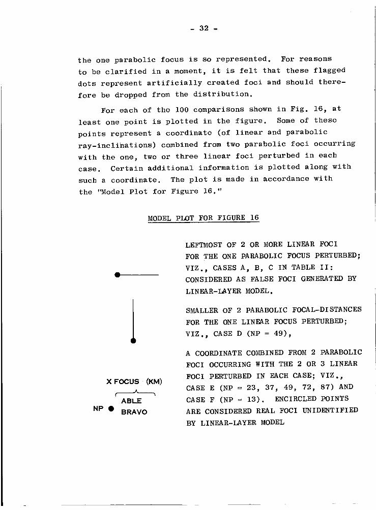
the one parabolic focus is so represented. For reasons

to be clarified in a moment, it is felt that these flagged

dots represent artificially created loci and should there-

fore be dropped from the distribution.

For each of the 100 comparisons shown in Fig. 16, at

least one point is plotted in the figure. Some of these

points represent a coordinate (of linear and parabolic

ray-inclinations) combined from two parabolic loci occurring

with the one, two or three linear loci perturbed in each

case. Certain additional information is plotted along with

such a coordinate. The plot is made in accordance with

the "Model Plot for Figure 16."

MODEL PLOT FOR FIGURE 16

A

W

X FOCUS • (KM)

ABLE

NP • BRAVO

LEFTMOST OF 2 OR MORE LINEAR FOCI

FOR THE ONE PARABOLIC FOCUS PERTURBED;

VIZ., CASES A, B, C IN TABLE II:

CONSIDERED AS FALSE FOCI GENERATED BY

LINEAR-LAYER MODEL.

SMALLER OF 2 PARABOLIC FOCAL-DISTANCES

FOR THE ONE LINEAR FOCUS PERTURBED;

VIZ., CASE D (NP = 49),

A COORDINATE COMBINED FROM 2 PARABOLIC

FOCI OCCURRING WITH THE 2 OR 3 LINEAR

FOCI PERTURBED IN EACH CASE; VIZ.,

CASE E (NP = 23, 37, 49, 72, 87) AND

CASE F (NP = 13). ENCIRCLED POINTS

ARE CONSIDERED REAL FOCI UNIDENTIFIED

BY LINEAR-LAYER MODEL

- 33 -

The perturbation case number 'TP" is written just to the

left of the point. This number comes from the leftmost

column of Table V, (p. 177). To the rightside of this

point are written the focal distances, in kilometers,

according to the two methods compared for representing

the atmosphere. The upper-right value (called '%ble"

in the model plot) is the linear focal distance; the lower-

left one (called "Bravo"), the parabolic focal distance.

Perturbation-case number 71 yields two parabolic

focal-distances for the one linear focus perturbed. The

two plotted points representing this case may be found in

the lower- and upper-right parts of Fig. 16. This case

is referenced as "D" in Table If. For the parabolic

model's initial ray inclination, the smaller value is

represented by the dot bearing the flag flying upward.

This focus is considered to be real, unidentified by the

linear method.

Then, there were five occasions in which linear and

parabolic loci (in the vicinity of the next-nearest, max-

type focus being considered) occurred in pairs -- see

Case E, listed in Table II. These five are perturbation

cases 23, 37, 49, 72 and 87 (the properties of which are

listed in Table V of this report).

In each of these five cases, the two pairs of loci

correspond in Fig. 16 to four points which form the corners

of an imaginary rectangle. For example, take perturbation

case 87. In the lower left of Figure 16, there is a

"corner" whose linear and parabolic distances are 8.2 and

7.8 kilometers respectively. (In the model plot, '_ble"

stands for the plotting position of the linear distance;

"Bravo," for the parabolic one.) In the lower right, there

is a corner having a linear focal-distance of 30.6 km

compared to a parabolic distance of 7.8 km. In the upper

- 34 -

left, there is a corner for which the linear focal distance

is 8.2 km compared to 34.5 km for the parabolic focal

distance and so on. In this case only the lower left and

upper-right corners represent what are considered to be

valid comparisons, according to the focal distances. The

other two points of perturbation-case 87 are illogical

comparisons. The same sort of selection would apply to the

other four cases under "E" in the inset table.

For perturbation-case 13 -- "F" in Table II, the linear

method produces three maximum-type loci in the 28-31 km.

range, to two such loci in the 34-35 km interval by the

parabolic method. These loci correspond in Figure 16

to points which form a rectangle, three points to one side

and two to an adjacent side, etc. Selection of correspon-

dence here is more difficult than in Case E. But, linear

(32.4 km, 18.4 ° ) with parabolic (33.8 km, 19.1 °) makes for

the combination with minimal differences in rays and their

focal ranging. The other might be linear (31.3 km, 19.8 ° )

with parabolic (35.4 km, 21.4°). By such selection processes

one might reject the flagged and encircled dots, leaving a

small, tight cluster of points at the upper right in Fig. 16.

In Figs. 14-16, the point C represents the next-

nearest, maximum-type focus as it occurred on the occasion

of the initial atmospheric state, which is shown in Figs.

iI and 12. On this occasion, this focus by the linear

method is LL; by the parabolic method, PP. These may be

found at the left and the right in Fig. ii. While the

correspondence between L and P seems apparent by their

proximity, it is not at all convincing between LL and PP.

In the 5-km interval between LL and PP, there occurs both

L and P.

- 35-

From Fig. 12, it can be now verified that LL and PP

are foci of the maximum-type. The PP is at the upper

right; LL at the lower left. Fig. 12 reveals some other

interesting characteristics about LL and PP.

The focus-factor varies inversely with dr/d_o. Hence,

negative lapse-rate discontinuities at data-points along

a linearized sounding of the propagation speed for sound,

each create somewhere a sound focus. In Fig. 12, the

lower-left inset is a portion of the sounding of wind-

and sound-speed, v = u + c, for the atmospheric condition

being considered. The data points, represented by small

circles, are joined by intersecting, straight lines, in

the customary way. The data-points M' and R' are positive

discontinuities in the sounding.

Along the dashed r(_o)-Curve below this inset sounding,

the breakpoints M and R correspond to the data points M'

and R'. The heights H at which rays reaching M and R top

out are plotted just below points M and R. These are the

heights of the data levels M' and R'. With increasing

initial-inclination, the slope of the r(_o)-Curve abruptly

backs (i.e., turns counterclockwise) at M' and R', from

negative to strongly positive. There, the discontinuity

in dr/d_o is positive, as indicated by the signs in the

figure. Positive discontinuities of dr/d_o occur with

positive discontinuities in -dr/dz.

In the sounding curve, positive discontinuities at

successive data points introduce along the r(_o)-Curve

adjacent discontinuities which are also positive. Between

such adjacent breaks the r(_o)-Curve must hump to a maximum.

The LL is just such a hump between M and R. The LL, then,

is a maximum-type focus, a false one created by linearization

of the observed atmosphere, in which successive data-points

both have positive discontinuities in the negative lapse-

rate of propagation speed.

- 36 -

In Figure 12 the ray landing at the max-type focus

LL tops out at 4166 meters, the level LL'. The ray landing

directly at the maximum-type focus PP zeniths out at 4448

meters, which is the level PP' along the parabolic sounding,

inset in Fig. 12. The focal intensity of LL is 105.192 DB,

compared to 101.314 DB for PP. The linear focus (19.925 °,

29.988 km, 105.192 DB, 4166 m) thus corresponds to the

parabolic focus (21.705 ° , 34.979 km, 101.314 DB, 4448 m),

with small difference in elevation, range, intensity and

height. Based upon such numerical criteria only, a match

between LL and PP might well be called for. This is just

the sort of matching which has been executed by Figs. 13-16.

As a matter of fact, this is the only matching permitted

because of the linear-layer method.

A mental operation, however, is now suggested for

application to the dashed r(_o)-Curve in Fig. 12. The

break-points M, R, S, and T are to be smoothed out. The

resulting curve would resemble a sinusoidal half-wave,

with a trough in the middle and a ridge toward the right

in Fig. 12. This trough would call for a minimum-type

focus around 29.5 km out and a maximum-type focus at

about 31.5 km. These foci would agree physically with the

P and PP, respectively. But, the positive discontinuities

M and R preclude the recognition of the minimum-type focus,

while the negative-type discontinuities S and T make it

impossible to give recognition to the maximum-type focus

envisioned there in the grand trend of the dashed r(_o)-Curve°

1.5 SHORT-PERIOD FLUCTUATIONS IN DISTRIBUTED SOUND

Short period fluctuations in the atmosphere do affect

the distribution of the propagated sound, such as shown

in Figure 11. But, such changes are not accessible through

the routine observational techniques for sampling the

atmosphere. They could probably not be made available even

- 37 -

WO

0

I!

II

!#

II

I

!I

II

I!

II

//

I

!I

!Ill

1.9 S I I_i. I I I

""*"'*".,,......,.,.,.,,.. %,% t

_ a --I i i_D o o

I

_.¢I

I

II

.¢!I

!!

II

!I

I/ s

/ I, ,1/ t

/ /! /

I II s

I

I

I II

I/

II

!/

/I

k\

_JJ

fI

I l i

I

I/

oI,q

W

o

I-_. W

_,.=_oo_

__z=

o__o

I

-II1_ .

_zldl -

_0_

8E"'_"z_l_OC3Z_

-- LiJL_I-

",., q

--WZ_"_0_

- 38 -

by the state-of-the-art observational techniques.

Discrete sampling therefore limits time- and spatial

information about the true turbulent continuum of the

sound-propagating atmosphere.

At any place, such changes may be nevertheless approx-

imated by perturbing the atmosphere in such a way that the

continuum of the small-scale changes so introduced is

physically compatible with the climatological experience

for that location. Such a process has been applied to a

selection of certain observed initial states of the atmosphere.

A large number of such fluctuated states of the atmosphere

thus approximate the observed information that would be

available from a very dense array of aerological observa-

tions made at very short intervals of time. Then, each

perturbed state can be reconstructed by well defined fit-

ting processes. This study compares two such fitting

processes. The comparison is made in terms of the sound

propagated according to the fitting processes used. In

this study the two fitting processes compared, of course,

are the linear fit with a parabolic one.

From a large number of such short period fluctuations

made of a selected atmospheric condition, the central

tendency and variability of the distributed sound are shown

in Figs. 17-23. The means and extremes in an azimuthal

distribution of sound intensity are shown in Figs. 17, 18,

21 and 22. Variability is given by Fig. 23. Between the

two methods for diagnosing the distribution of propagated

sound, differences are summarized in Figs. 19 and 20.

Fig. 17 summarizes the sound distribution for 100

small-scale, perturbed states of the atmosphere. The

radial distribution of sound intensity at the ground has

been determined from the linear method of straight-stepped

- 39 -

representations of observed atmospheric layers. This is

the customary way used for representing the atmospheric

sounding. In this figure, the distribution lies along

the 45°-azimuth from a 204-DB source at Huntsville,

Alabama. It is based on atmospheric situations, perturbed

out of the basic or initial condition as observed at 1636

CST on February 27, 1964.

In this figure, the abscissa is radial range (r)

in kilometers; the ordinate, sound intensity (DB). The

sound intensity has been calculated at one kilometer inter-

vals (the encircled points). Just above these points,

certain numbers are written along the "mean" mid-curve.

These indicate the number of occasions on which sound did

return directly to the ground at the range corresponding

to each labeled point. The maximum number of such occasions

possible would be the i00 different atmospheres that to-

gether constitute the artificial sample made over a short

period of time. We shall now consider the frequency dis-

tribution of direct ray landings as shown by these numbers.

1.5.0 IN OCCURRENCE

From around 13 km. and out (to around 31- or 32 km.),

the number of returned rays (out a hundred possible) drops

off (Fig. 17). Only about one-eighth of the time did sound rays

return into this range interval. This oftentimes "silent"

zone is associated with a ray bifurcation. Within this

zone, a dozen or so cases do return sound there. Over these

limited cases, moreover, a sound maximum E is created at

16-17 km. out from the source. The silent-zone, ray-bifurcation

and sound-maximum E -- together constitute the topic of the

following considerations.

- 40 -

From 13- to 32-km. out, the silent zone results fromrays that zenith out at the top of a lifted inversion in

the atmosphere. This inversion is located just above the

ground (see the inset in Fig. 6). In this case the silent

zone is the artificial result of a local-maximum discon-

tinuity in the linearly represented sounding of wind- and

sound-speed. In creating a silent zone, one effect of

the straight-stepped representation of the inversion is

ray bifurcation.

In the basic, unperturbed atmosphere, the magnitude

of this inversion is Av = _ (c + u) = 13 meters per second

through a depth of just 400 meters. It is therefore a

rather strong inversion. Over time variations of a small

scale introduced into this basic atmosphere, this inversion

should persist.

The ray geometry of the sound propagated by the basic_

unperturbed state of the atmosphere has been determined.

But, such ray geometry of the sound that is propagated

state by each perturbed atmospheric state has not been

found. From a random selection of atmospheric states most

of the time the silent zone would evolve from a ray geometry

associated with an inversion both of which (ray-geometry,

inversion) are similar in physical principle with the ray

geometry and inversion of the basic or initial atmosphere.

The following discussion is explicated in terms of the

geometric values of sound rays associated with this inversion

in the basic atmosphere. Whatever are the numbers involved

in this ray geometry_ or in similar geometry, they are

effective in describing the physical conditions out of which

the silent zone generally arises.

For a graphical representation of the basic or initial

atmospheric sounding of wind- and sound-speed, reference

may be made to the sounding inset in Fig. 6 of this report.

- 41 -

And, the rays bifurcated by the inversion being considered

in connection with the silent zone are those listed in

rows 33 and 35 in the righthand of Table IV-Able, p. 107,

of KN-67-698-1.

Whenever it occurs, the silent zone is the mechanical

result of a local-maximum discontinuity in the straight-

stepped representation of atmospheric wind- and sound-speed

along the iocal vertical. The combined value v of wind-

and sound-speed is less both immediately above as well as

below this wedge-shaped discontinuity.

In the straight-stepped representation of the initial

or unperturbed atmospheric sounding, the height of this

wedge-shaped inversion is 0.894 km., which is the height

of the data-point at this local maximum in the sounding

curve. The particular ray that tops out at this inversion

height is the one which leaves the source with an initial

inclination there of 14.878 °. Remaining intact as a single

ray, it reaches its zenith exactly at the top of the

atmospheric inversion represented by straight-stepped layers.

At this wedge-shaped zenith, this ray splits or bifur-

cates into two rays. From that zenith point, the two rays

follow separate paths away from the sound source. One part

of this split ray returns to the ground at a range of 13.085 km.

Topping out at the level of this maximum cone part of

this ray has thereafter been returned to the ground, straight-

away. But, the other part of this ray (that has also

leveled out at the top of this wedge-shaped inversion) there-

after is "bent" upward, as it penetrates atmospheric layers

above the inversion where wind- and sound-speed decrease with

increasing height (positive lapse-rate).

Still higher, however, superjacent layers again have

negative lapse-rates of wind- and sound-speed. These layers

- 42 -

start "bending" downward this upward ranging part of thebifurcated ray. Eventually, it therefore zeniths out again,at an altitude now of 3.812 km. This is 2.918 km. higherthan the inversion discontinuity at which the ray first split

into the two subsequent paths and at which the other part ofthe ray finally topped out.

Having negative lapse-rates of wind- and sound-speed,

these superjacent layers aloft return the upper part of thebifurcated ray to the ground 55.988 km. from its source.Thus, there is a skip-zone of 42.903-km. wide, between thetwo landing points of the one ray that is bifurcated by thewedge-shaped representation of the atmospheric inversion.

The case of the skip-zone thus illustrates the general-

ization made in the previous reports that dr/d_o is negativelydiscontinuous at a local maximum in the linearly representedsounding of wind- and sound-speed. (KN-66-698-1F and KN-67-698-1). At a local-max discontinuity in the linear sounding

of wind- and sound-speed, the lapse rate is also negativelydiscontinuous. Thus, associated negative discontinuities in

the lapse-rate of the straight-stepped sound and in dr/d_ocorrespond to the silent, skip zones in the propagated sound.

However, as Figure 17 indicates, about one-eighth of the

time this 43-km. zone of frequent silence is otherwise filled

with sound from rays that do land directly therein. (In the

computer program from which these results were obtained, the

Subroutine FIT is so written as to yield, for each case of the

ray bifurcations, a zero value of sound intensity at those

requested distances which fall within the skip zone of each

perturbed state of the atmosphere). From Fig. 17, it is

therefore evident that, from one perturbed state of the atmos-

phere to another, the skip-zone either changes in length and

position or vanishes occasionally. From occasion to occasion,

- 43 -

rays enter there in one of at least two ways and fill out

part of the skip zone with sound.

First, in any given atmospheric situation, other rays

from the sound source could land directly in at least a

part of the skip-zone interval created by one part of the

atmosphere, such as the inversion just considered. Second,

the particular inversion creating the skip-zone could be

fluctuated out of existence. In the real situation, such

a disappearance would be realized through the burning-off

of a nocturnal inversion as a result of solar heating of

the ground, etc.

In the unperturbed basic state of the atmosphere con-

sidered in this example, the situation illustrates the first

way. (It will be recalled that the direct landing distance

of the 14.878°-ray skipped from 13.085- to 55.988 km. This

jump results from the wedge-shaped inversion-lid at 0.894 km.

altitude). Actually, both the near- and far-ends of the

skip zone are filled in with rays returned there from other

atmospheric layers than the lifted inversion.

The first 0.890-km is filled with rays returned there

from the topside of a shallow ground inversion. Beneath

the lifted inversion, referred to as E, there is another,

shallow ground inversion with its top at 0.106 km. (see the

inset of Figure 6). The straight-stepped representation of

this inversion bifurcates the 4.336°-ray, the upper part of

which lands out at 14.975 km., within the skip-zone created

by the wedge-shaped representation of the lifted inversion.

With an initial inclination just above 4.336 °, rays pene-

trate the superjacent layers with a positive lapse-rate of

wind- and sound-speed and, from there, are returned directly

to the ground landing in the skip-zone inside 14.975 km.

- 44 -

Their direct landings move closer toward their source with

their increasing initial-inclination. In the case of the

basic unperturbed atmosphere, they fill the first 0.890 km.

of the skip-zone created by the bifurcation of the 14.878 °-

ray. Generally, in the I00 samples of actuated atmospheres,

the F-interval (Figure 17) of the skip-zone if frequently

invaded in this way with rays landed directly there by the

ground inversion. As seen in this F-interval, the atmos-

pheric cases with direct ray landings drops off from i00

to 98 at 14 km., to 54 at 15 km. and 21 at 16 km.

In the basic state, at least the last 36.747 km. of the

skip-zone are also filled with sound from rays landed there,

in this instance from upper atmospheric layers. The vertical

ray-fan from 14.878 ° to 21.272 ° of initial inclination lands

in this far end of the skip-zone (as does the fan above it).

In the unperturbed basic-atmosphere, only a 16.156-km.

stretch remains "silent". Since the observed sounding was

limited to the first five kilometers of the atmosphere, one

cannot say, moreover, whether or not other layers above that

5-km. limit would have contributed to the complete elimina-

tion of the skip-zone. At any rate, it is quite possible that

small time variations in this basic atmosphere could result

in the skip-zone being completely filled with direct landings

of rays returned by the first five kilometers of the perturbed

atmosphere. As a matter of fact, this did happen 8-to 13% of

the time, according to the results shown in Figure 17 and

Figure 21, which is a radial extension of Figure 17.

It is therefore not apparent what ray-geometry is assoc-

iated with the sound maximum E, found one-eighth of the time

in the skip zone. But, from Table V and Figure I, 7 and 13,

the conclusion can be made that the E is at least not assoc-

iated with a sound focus. Therefore, it may be surmised that

it is associated with a "false-type" focus that results out

of the straight-stepped representation.

_L_I

O

- 45 -

mw

IL

n u

I

O

p

I

OO

ON

O

cO

ILlr_

u_n,

3:nU3O

I-

W3CI-

7

U_ZoI-

_1

U

cn_II-

_IIAI_1o

-I-ol-on,

,,P.or.

_aII1 Z

clul

z_

i i I

- 46 -

m

0

0

O_

hlII

IL

0

W

m_m°_m_

DWOU

ZDmml

og.o

O_wm W=

_ oU

_-_.N

ZZZO_."'0<

=_zE_I0_ Jm,_

Zo_ _

7- + I T

- 47 -

Whereas the E maximum is not associated with a sound

focus, in Figure 17 the peaked maximum L obviously is.

From one perturbed atmospheric state to another, a minimum

type focus is created by rays inclined ii-14 ° from the source

and returned from within the lifted inversion layer directly

to the ground 7-9-km. out. where their landings first range

inward then out. (At this focal range, the same ray-fan

occasionally creates also a max-type focus in some of the

perturbed atmospheres - cf. Figures 1 and 13).

This minimum-type focus also shows up in the sound dis-

tribution as determined by the parabolic model (see P in

Figure 18). Corresponding to the sound maxima L and P in

Figures 17 and 18, the location of the minimum-type loci

L and P there for the basic state is shown in Figure 5.

But in Figure 18 there is no evidence of another sound

maximum out around 17 km., corresponding to E in Figure 17.

Other comparisons between Figures 17 and 18 may be now noted

more effectively in Figures 19 and 20.

1.5.1 In (Means and) Extremes

As shown in Figure 19, in the radial interval AB, the

parabolic model results in a greater limit or range to the

intensity of the sound distribution than does the linear

representation. But, in the radial interval BC, this dif-

ference is reversed between the two models. This radial

interval AB is also indicated in Figures 17 and 18. No

explanation as to the greater DB-range in the parabolic model

there appears in these figures.

In the vicinity of the sound maximum E (Figure 17), the

intensity of the sound distributed according to the linear

representation is some 20 DB higher than according to the

parabolic model (see Figure 20). This increased intensity

is over three times the a_erage excess of that for linear

loci over that for the corresponding parabolic foci, as

found in Figure 3.

- 48 -

ADB

25

20

15

I0

15I I I I I I I I I

20 25(KM)

FIGURE 20

SOUND--INTENSITY DIFFERENCES BETWEEN LINEAR AND PARABOLIC

DISTRIBUTIONS OVER 100 SMALL--SCALE VARIATIONS IN AN ATMOSPHERIC

STATE. FIGURES 17 AND 18 GIVE THESE DISTRIBUTIONS. IN THE SENSEOF LINEAR LESS PARABOLIC,THE MAXIMUM,MEAN AND MINIMUM DIFFERENCES

EACH INCREASE UPWARD,WHILE THE AZIMUTAL DISTANCE GOES TO THE RIGHT.

- 49 -

j _'_

uhv

!I

I I II I I

I I I

I _ _I ! iI I !

I I I! I I

J

\ Is.

I "'"

Ii.

?I I ,.

! I b.

I tI I

(_ i, "_l-_ )

oI

I ,%

' _I ii i

!i i

i !

I \

U3 00 0

I

//

//

/

|

o0o

o

-- It3

wn.,

ILlm

b.0

Zo_I-

I--Z

mul

hill

,,,EZ

-_oul_Z

t__Z

II_l-n×

Ul

I-J

z__--N

z3Z0"{

Is.-OLd

D_>'DE(3

_m

z

i11 ul_-1-i1_ !1.I-mmO

- 50 -

But, the sound intensities given in these two figures

are not evaluated in the same way or for the same thing.

In Figure 3 the sound intensity comes from the Brekhovskikh

expression and is valid just at the position of a particular

sound focus for a particular atmospheric situation. As

referred to here in Figure 20, the sound-intensity value

("mean" curve) is from the well-.known expression given by

0rvel E. Smith averaged over i00 atmospheric samples. For

each sample, this value is interpolated at unit-kilometer

intervals from intensities at adjacent ray-landings, usually

but a few meters apart. Since focal spikes of sound in-

tensity extend over only a short radial distance, and since

the tabulated distances are far apart, it is unlikely that

the effect of any focal intensities themselves will show

up in any of the curves of Figure 20.

Over the radial distance BC, the greater DB-range in

the linear representation than in the parabolic (Figure 19)

one comes with (a) increase there in the difference between

the two methods in their maximum sound-intensity along with

(b) a decrease in the difference between them in their mini-

mum sound-intensity, where these differences are in the

sense of linear less parabolic; this is shown in Figure 20.

The discussion now proceeds to consider the sound dis-

tribution farther out. Figures 21 and 22 are radial or

azimuthal extensions of Figures 17 and 18. Attention is

now directed there to the sound distribution being associated

with the linear loci L and LL and the parabolic foci P and

PP. For the unperturbed, basic atmosphere, these loci are

shown in Figure ii. Their definition is given in Figure 12;

Smith, Orvel E., "Far-Field Sound Propagation as Relatedto Space Vehicle Static Firings", presented to the FifthConference on Applied Meteorology of the American Meteor-

ological Society: Atmospheric Problems of Aerospace

Vehicles, March 2-6, 1964, Atlantic City, New Jersey,

p. ii.

- 51 -

Z

N

ILl

ZO_F---

n_z_w_

0_Zu_o-lz

II_Ul

0'_

Ez

N R

Z--

0z-

0(1:

Ii_'r

--Idl-m-in..m_

W

<0

- 52 -

L and P are minimum-type foci; LL and PP, maximum-type.

Over the i00 samples of short-period change, their fre-

quency of occurrence is summarized in Figures 7 and 13.

(Figures 7, Ii, 12 and 13 have already been discussed).

In Figures 21 and 22, the positions of these four loci

are given by the points C L, CLL, Cp and Cpp respectively.

These foci all show up in the maximum intensity

curves. Because of their overlapping range in distance,

the L and LL smooth out into a single maximum in the mean

intensity. The PP does not peak separately in the mean

intensity.

In Figures 21 and 22, the sound intensity represented

by both the three curves in each figure and the four C-

subscripted points in both has been evaluated in exactly

the same way. That is, the value represented by the en-

circled points along these curves and the C-subscripted

points has been computed according to arithmetic statement

590 in Subroutine TENSITY (see p.146). This statement

executes the expression presented by O. E. Smith, et. al.

It is emphasized that, at least in principle, this value

has point validity only. Thus, along the curves, the

sound intensity is valid only at the unit-kilometer

locations marked with the encircled points. Indeed it is

quite misleading to have connected these points with curves,

as has been done in these figures. Between adjacent points,

the connection implies a certain continuum of sound inten-

sity as defined by glabrous curves. This is not so.

Actually, along these curves, the "point" values do

have some spatial extent. From the TENSITY-statement 590,

Subroutine FIT finds the sound intensity at requested dis-

tances (i.e., unit-km, positions).

- 53 -

The FIT performs a quadratic interpolation of in-

tensity from adjacent ray landings, which at most are

but i00 meters apart. In spatial extent, then, the

sound value at these points along the curves might be

considered as being representative across a few tens of

meters of radial distance, at most.

The curve-joined points represent mean and extreme

values of sound intensity from i00 perturbed atmospheres.

Along the mean curve, each such point represents a mean

value averaged for the number of atmospheric cases which

returned direct rays there. This number is written just

above the point.

Along the max-curve, each point represents the

largest value of sound intensity that occurred there out

of the number of cases just mentioned. The same for the

min-curve.

But, of course, the max curve is not an intensity

envelope for the sound distribution at the ground along

the chosen (450-) azimuth. Focal amplifications of sound

are very limited in horizontal extent. From Fig. 5, for

example, it can be seen that the focal spikes of sound

intensity have a lateral extent of not more than around

20- or 30 meters. Outward from the source, sound foci are

very narrow. Since the local amplification of focal sound

extends across but a few meters, it is not likely that, out

of just i00 perturbed atmospheric states, a focus happens

to fall exactly at one of the 40 unit-kilometer distances.

Between adjacent points connected by the max-curve, then,

there probably occur numerous occasions in which the local

value of sound intensity lies "above" the max-curve.

One can therefore not be perplexed by the fact, for

- 54 -

example, that in Figs. 21 and 22, points CL and Cp lie onthe higher DB-side of the curve representing the greatestsound-value encountered at unit distances in the sample of

i00 perturbed atmospheres. Indeed such points may exceedin value the max-curve by as much as 30 DB.

Around the focal region 30-35 km. out, then, the max-curve should take on numerous, flageliform spikes -- becoming

there hairy-like in appearance. For the 100 sampled atmos-pheres, the radial extent of the minimum-type focus there inFig. 21 is indicated by the horizontal, broken dimensional-arrow labeled "(Fig. i0)."

As a matter of fact, due to the max-type focus thatsometimes also occurs in that region, numerous spikes shouldalso occur all along the 25- 40 km. interval, marked out bythe horizontal, solid dimensional-arrow labeled "(Fig. 14)."

In both Figs. 21 and 22, the min-curve is probably themost representative of the three curves. The min curve ismore or less an intensity envelope for the lower DB-limitof the radial sound distribution along the ground. The most

striking result from comparing Fig. 21 and Fig. 22 is the25-DB difference between their min-curves beyond 28 km. out.

In the parabolic model, the "min-curve" remains flat, peakingonly slightly at 28 kms. On the otherhand, in the linearmodel, the min-curve raises to a sharp maximum at 28 kms. andthereafter remains "plateau-ed" close to th_ mean curve and

straight.

This striking difference is indicated in Fig. 20. Toward

the right in this figure, the min-curve rises abruptly.Even beyond the radial extent of this figure, the excess of thelinear min-value of sound over that of the parabolic methodremains around 21-25 DB, out to at least 40 km. On the other-

- 55 -

Q

hand, both methods yield nearly the same values of mean-and max-sound, beyond 30 km. out.

As a rule, the linear method yields average values ofsound too high in regions where it would bifurcate sound rays(18- 30 km. in this example). On the other hand, it is not

responsive to situations resulting in weak sound (28- 40 km.).

In Figs. 21 and 22, the vertical dimensional arrows show

the range in the intensity of focal sound as obtained from the

Brekhovskikh expression. This value is evaluated by arithmetic

expression 630+2 in Subroutine TENSITY. The broken arrow in

each figure pertains to the min-type focus occuring in the

20-24 km. interval; whereas, the solid one, max-type focus

in 25-40 km. interval for the linear method and the 33-39 km.

for the parabolic method. It is to be remembered that these

vertical arrows represent sound intensity which is evaluated

differently than that represented by the C-subscripted points

and the curves.

In Fig. 21 no difficulty should be therefore assigned to

the fact that these vertical arrows extend below the min-curve.

It is interesting, however, that the focal ranging in both

spatial extent as well as sound intensity is greater by the

linear method than by the parabolic one. This is evident in

the greater length of the dimensional arrows of the same type,

in Fig. 21 compared with Fig. 22.

It is reminded, incidentally, that the spatial ranging of

the foci shown by these arrows is the same for either the

Brekhovskikh expression or the one presented by O. E. Smith.

A comparative evaluation of these two expressions has been

the result of an analysis previously reported by Kaman Nuclear

(ref.3). Even so, it might still be mentioned now that, in

the Monte Carlo evaluations carried out in this current study,

- 56 -

the focal sound intensity is more readily evaluated by the

Brekhovskikh expression than by the Smith expression.

Primarily for this reason only, Program ALLSOND, on which

the results of this study are based, has made use of this

wave-interference expression of Brekhovskikh for evaluating

focal intensities. But, this program also employed the

Smith-expression for getting sound intensities at requested

distances.

Figs. 18-22 were primarily concerned with comparing the

two methods in terms of the sound intensity at requested dis-

tances. Here, the concern was with some preliminary aspects

of sound variability. For these figures, in particular, the

range of variability assigned to the atmospheric parameters

was that which would take over a span of just a fraction of an

hour. Although small, this amount of atmospheric variability

nevertheless did yield certain significant variations in the

distributions of the propagation, as the discussion of these

figures revealed. First, the discussion considered whether

or not there would be any rays returning directly to a given

distance. It was seen that the presence of directly return-

ing rays at a given point was essentially a probability pro-

blem. The probability was large at some distances, small at

others. Second, the discussion of these figures summarized

some results as to the extremes in such variations about their

central tendency, when direct rays did return at the given

distance from the source.

1.5.2 IN VARIABILITY

From such information about the occurrence probability

of sound, its means and extremes, the discussion can proceed

now to the sound variability itself. Fig. 23 shows the

standard deviation (DB) in the linear and parabolic sound

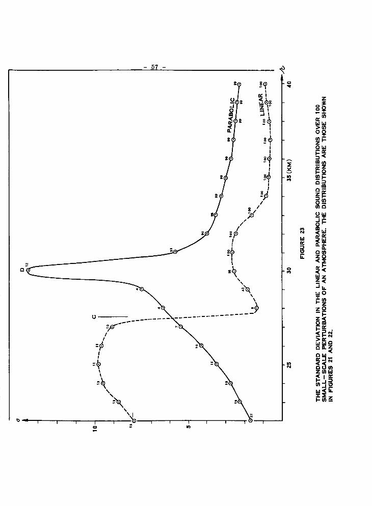
- 57 -

I

\

i , _) , | i ! ! |_. liP/

0'qr

_n

z0','p=

m I1_i-.

jh.mOz

z9--I-

Z_l,i

..1_W_b.

- 58 -

distributions over a hundred of these small-scale perturba-

tions of an atmosphere. Here, the spatial distributions

are those shown in Figs. 21 and 22.

From C outward, in Fig. 23, the parabolic method

results in a greater sound variability than does the linear

method. From Fig. 21, it can be seen that this position C

is where the min-value according to the linear method rises

abruptly to a high, plateau. Beyond 35 km., the parabolic

method yields a standard deviation three and one-half times

that of the linear method. In between, the greatest standard

deviation was 12 DB, at position D. According to Figs. 22 and

23, the parabolic method returned rays directly to this posi-

tion D only an eighth of the time. At each one-km, interval

along the curves in Fig. 23, is plotted the number out of the

i00 cases with sound propagated directly to that point. But,

whenever, they did return to the vicinity of this position,

it was probably near the next-nearest minimum-type focus,

although there were occasions when the sound itself was quite

weak at this position.

In a general way, from Fig. 23, it appears that if the

likelihood of returning rays is not large, the standard

deviation of intensity of what rays are returned may be some-

what larger than otherwise. This apparent conclusion is

detailed in Figs. 24-26.

These figures continue the comparison of the two methods

in terms of the variability in sound distribution. The dis-

tributions are those shown in Figs. 18-22. The difference in

the number of direct rays returned is shown by the dashed

curves. The difference is in the sense of linear less para-

bolic. The dashed curve references the vertical scale at the

right in these figures. In the same sense, the solid curve

- ,_,(:I- AN

90AO"

6-"

(on)

5-

4-

3

/I

II

I!I

®

Ic\

®

80

70

60

, , / \ ,oo- _ "40

--1 - i - 30

-,- '\\ \

-3 - c / _\®

..e/" E

_I.... ,,e---e--.-e--...e--"

---4-

®_ _...O

--6-

/I

I

LlO

I I I I I I I I i i i _'_'-"_'z I -SO

1 2 3 4 5 6 7 9 I0 11 12_KM)13 14

--10

--20

--3O

--4O

IIIIIIIIIIII

D t

!

8

--7

--8

--9

--I0

FIGURE 24

VARIABILITY IN SOUND DISTRIBUTION COMPARED BETWEEN THE TWO METHODS.FOR DETAILS AS TO THE SITUATION INVOLVED IN THIS COMPARISON,SEEFIGURE 1. DIFFERENCES SHOWN HERE ARE IN THE SENSE OF LINEAR LESSPARABOLIC. THE DIFFERENCE IN STANDARD DEVIATION OF SOUND INTENSITYIS GIVEN BY THE SOLID CURVE,WHICH REFERENCES THE LEFTHAND ORDINATE--SCALE. THE DIFFERENCE IN THE NUMBER OF RAYS RETURNED IS GIVEN BYTHE DASHED CURVE,WHICH REFERENCES THE RIGHTHAND ORDINATE. INCREASINGTO THE RIGHT AT ONE--KILOMETER INTERVALS,THE LOWER SCALE SPECIFIESTHE RADIAL DISTANCE OF THE DIFFERENCES. FIGURES 25 AND 26 ARE RADIALEXTENSIONS OF THIS FIGURE.

- 60 -

--4

--5

--6-

--7

--8

--9

--10

14

FIGURE 25

DIFFERENCES IN THE VARIABILITY OF SOUND INTENSITY AND IN THENUMBER OF RAY LANDINGS. FOR FURTHER DETAILS, SEE FIGURE 24.

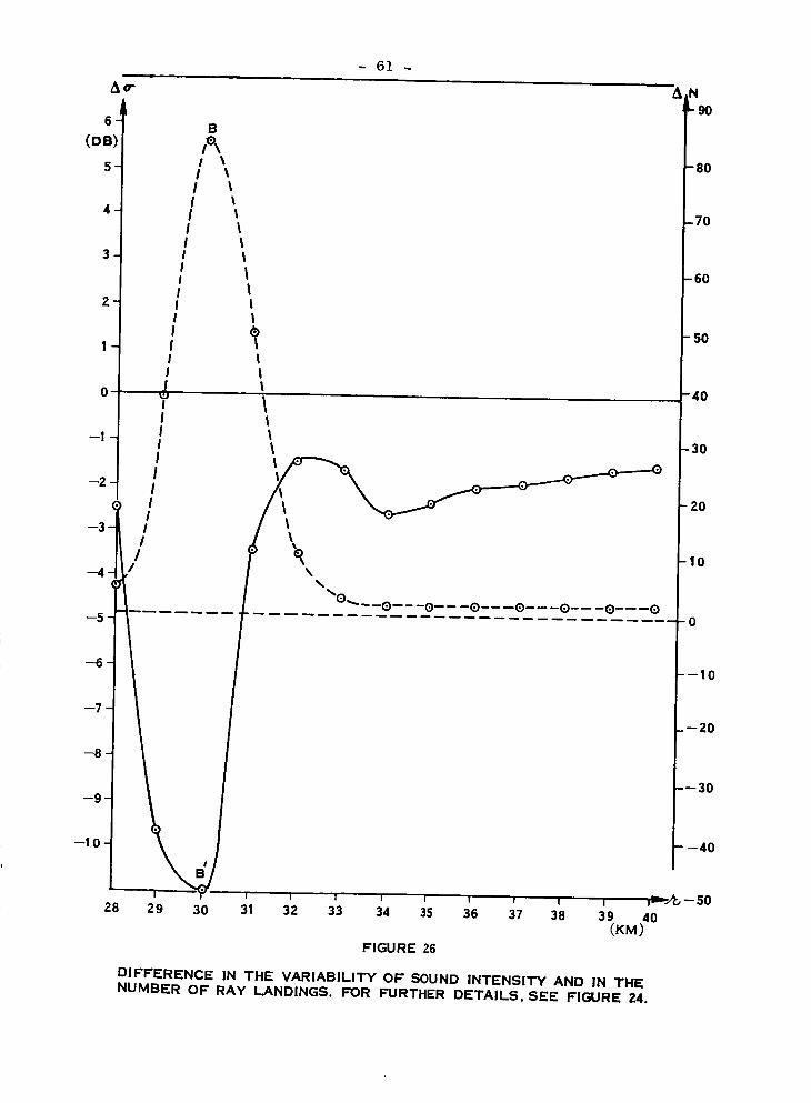
- 61 -

Ao"

6"

(DB)

5

II

IIIIIIII!II

//

B

II lII lI ll It lIl l! tI t

,II I

II

\

_N_-90

-80

-70

-60

- 50

-40

-30

20

10

0

--10

_--20

---30

- --40

28 29 30 31 32 33 34 35 36 37 38 39 40(KM)

FIGURE 26

DIFFERENCE IN THE VARIABILITY OF SOUND INTENSITY AND IN THENUMBER OF RAY LANDINGS. FOR FURTHER DETAILS, SEE FIGURE 24.

- 62 -

gives the difference in standard deviation of sound

intensity between the two methods. The solid curve

references the vertical scale along the left. Increas-

ing to the right at one-kilometer intervals, the lower

scale specifies the radial distance of the differences.

Figs. 25 and 26 are radial extensions of Fig. 24.

For example, 10 km. out, the standard deviation of

sound intensity by the linear method is 1.228 DB and 0.872

by the parabolic method. Their difference is + 0.356 DB

(point A in Fig. 24). Out of a hundred tries, the linear

method returns all rays directly to this position, while,

the parabolic method returns rays directly there everytime

but once. The difference is +1 (point A' in Fig. 24). When

nearly all rays are returned, in this situation both methods

seem to yield an equally small variability in the intensity

of the distributed sound.

Another example, 30 km. out, the standard deviation of

sound intensity by the linear method is 2.570 DB and 13.519

by the parabolic method. Their difference is _ = 10.950 DB.

(point B' in Fig. 26). 95% of the time the linear method

would return rays directly there, but the parabolic method

would manage to get rays there only 12% of the time. The

difference in likelihood is therefore +83% (point B).

Together, Figs. 24-26 reveal a rather prominent and

significant feature: the curves deviate oppositely. Examples

of such departures in opposite direction are B, B'; C, C';

D, D'; E, E'; and F, F'. In other words, greater vari-

ability in the distributed sound goes with the method yield-

ing the less probability of directly returned rays.

Thus far in the comparison of atmospheres represented by

- 63 -

t_¢<Uz 20-

10-

0-

0

.Jo 10-K_<

20-D.

I'-I

A

l I

t l

6O

4Oat<Id

30 zJ

20

J

R : ' '-[-],,:I:, , lo

_.l ............. r__l ..I I._1 I r_

"11.....o10

20

U __ [3U -

,J

0

40at<

50

i°°l70

II

!

!

,' r;;;I I I I I

_.0.._..___,._r-] =_ _ == _ U !._j I I o J rl .._

....-.... ................., FIE]

;';''//i_'''_ ....... _"_"lo z7 , 3, 33 35 3 3, ,1

FIGURE 27

IN THE UNIT RANGE SPECIFIED BY____, THE OCCURRENCE PROBABILITY OF

(1) ONE OR MORE FOCI(PARTIAL), (2) A FOCUS (TOTAL). FOR FURTHERDETAILS SEE THE LEGEND TO FIGURE 1.

- 64 -

straight-stepped layers with those by parabolic-smooth

ones, for the most part the discussion has looked at the

sound distribution around the four loci that recur in the

chosen situation. But, in the final analysis, the vari-

ability of focal intensity itself should be of special

significance in comparing and evaluating these two methods.

The discussion, therefore, will now concentrate on the

intensity of focal sound, its occurrence probability, vari-

ability and radial distribution.

1.6 SHORT PERIOD FLUCTUATIONS IN FOCAL SOUND.

In Fig. 27, the bar-graphs show the likelihood of

occurrence of the four loci. Bar groupings for the mini-

mum-type foci are found in the upper-half of this figure;

bar groupings for the max-type, in the lower half. Foci

closest-in to the source are at the left; the next nearest,

at the right. Because min- and max-type loci each tend to

occur in the same vicinity -- one pair around 8 km. and

another around 30 km., Occurrence probability by type are sep-

arated in the figure. The frequency scale along the left

vertical applies to the max-type foci; the scale at the

upper right, to the min-type foci. Frequency of occur-

rence (in percent) is measured vertically from the hori-

zontal dashed-line: upward for atmospheres represented

by straight-stepped layers, downward for those by parabolic-

smooth ones. The horizontal scale at the bottom gives radial

distance in kilometers increasing to the right. Note that

this scale is fore-shortened between i0- and 25 km. For a

perturbed state of the atmosphere, represented by either

method, more than one focus of the same type occasionally

occurs within the same unit-kilometer interval. The likeli-

hood of this happening is given by the tipped portion of a

DB

I05

100.

95 _

90-

85-

80-

75-

70-

- 65 -

STANDARD DEVIATION IN ---P-_-_2.6INTENSITIES OF ALL MAX--TYPE FOCI FALLING WITHIN

THE SPECIFIED _ KM.INTERVAL* ----'_

I 2.or---II II I

_12_.5_LARGEST VALUE OF IN--TENSITY OF ALL MAX--

TYPE FOCI FALLING

WITHIN THE SPSCIFIEDI KM. INTERVAL.

I1

MEAN INTENSITY IN OB I

OF ALL MAX--TYPE FOCl

°,_.u_"R-,"._c',-F,T."_' '_.... --I

IIII

1 I

1

HUMMER OF MAX -- TYPEFOCI OCCURRING IN THE -----

SPECIFIED I KM, RANGE.

I II II I 1.2

---, r-7I I I

ii---I I (;7..J _-'_--'"_1 11

-;;l ! l i-"____

-4o-;_-_-_ _J---_ 'I

ISMALLEST VALUE OF

INTENSITY OF ALLMAX--TYPE FOCI FALLING

WITHIN THE SPECIFIEDI KM. INTERVAL,

ONCE WITHIN THE SPECIFIED! KM. INTERVAL FOIIt A GIVEN

ATMOSPHERIC STATE.

15

I , , i , . I , , , i _-J_J

25 30 (KM) 35

FIGURE 28

A DISTRIBUTION SUMMARY FOR MAX--TYPE FOCl OF SOUND PROPAGATION

IN 100 RANDOM PERTURBATIONS OF THE ATMOSPHERE REPRESENTED BY

STRAIGHT--STEPPED LAYERS. FOR FURTHER DETAILS,SEE THE LEGENDTO FIGURE 1.

- 66 -

DB

100 J

95-

9O

85

8O

0.2

22

1.9

26

12

2.3

T 0.3g:::=::N

2

75 , i i i i i i l i I

30 35 (KM) 40

FIGURE 29

A DISTRIBUTION SUMMARY FOR MAX--TYPE FOCi OF SOUND PROPAGATEDIN 100 RANDOM PERTURBATIONS OF THE ATMOSPHERE REPRESENTED BYPARABOLIC--SMOOTH LAYERS. FOR FURTHER DETAILS,SEE FIGURE 28.

- 67 -

few of the bars. For example, three per-cent of the time,

by the linear method, at least two min-type foci occur in

the interval between 31- and 32 km. (point A in Fig. 27),

when the atmosphere is represented by straight-stepped

layers. The overall occurrence is given by the total length

of the bars from the horizontal, dashed line.

Much of the results presented in Figs. l, 7 and 13 also

appear in Fig. 27. These may be reviewed. In addition,

some new information also appears. Consider the two bar-

groupings in the right half of Fig. 27; they correspond to

the location and occurrence of the next-nearest, max- and

min-type foci, as determined by either method. For these

two types of foci, which overlap along the azimuth, the

distribution of focal intensities is shown in the companion

Figs. 28 and 29.

Focal intensities are shown in Figs. 28 and 29. These

figures are distribution summaries for the next-nearest max-

type loci of sound propagated in 100 random perturbations of

the atmosphere. In Fig. 28, each perturbed atmosphere is

represented by straight-stepped layers; in Fig. 29, by

parabolic-smooth ones. These figures cover a ll-km, segment

of the 45°_azimuth from Huntsville. Beginning 24-km. out,

this segment in Fig. 28 overlaps approximately the first half

of that in Fig. 29. The vertical bars describe the ranging

of focal intensity over unit-kilometer intervals along the

azimuth. The intensity is evaluated according to Brekhovskikh

(ref. 1 ). Somewhere between the ends of the bars, a hori-

zontal line marks the intensity-value averaged for the number

of max-type foci occurring in the specified unit-kilometer

interval. This number is written below each bar. These

numbers have been represented by the bars referred to in

- 68 -

Fig. 27. The standard deviation in intensities of allmax-type loci falling within the specified 1-km. intervalis written above each bar.

Compared with one another, Figs. 28 and 29 reveal somevery striking differences between the two methods forrepresenting the atmosphere. Compared to the straight-stepped set of bars (Fig. 28), the variation in the para-bolic-smooth one (Fig. 29) is more regular in form and less

in extent. In the parabolic one, the ranging of focalintensity varies with radial distance in a quasi-Gaussianway; whereas, in the linear one, there is a great irregu-larity with focal distance in the ranging of Iocal intensity.

Table III-A gives a numerical contrast to this matter of a

probability distribution in the ranging of focal intensity:

TABLE III-A

In DB., the Ranging of Focal Intensity over the

Unit-Kilometer Radial Intervals in Each of

Which Max-type Foci Occurred

Linear Method Parabolic Method

0. O.563

0. 1.794

0. 7.434

(no focus) 7.768

25.9729.295 7.551

9.880 8.197

4.619 7.890

27.336 0.518

2.470 O.

O.

- 69 -

Regularity in form shows up in another way. With

the parabolic method, the mean unit-kilometer values of

focal intensity varies with focal distance also in a

quasi-Guassian way; whereas they do not, by the linear

method. This can be seen from the cross-hairs on the

bars in Figs. 28 and 29. Table III-B quantizes this

evidence as to the matter of regularity in spatial dis-

tribution of focal intensity.

TABLE III-B

In DB, the Algebraic Difference in the Mean FocalIntensity Per Unit-Kilometer Interval, the DifferenceBeing Taken from One Interval to the Next Outer Interval.

+ 0.017 -1.036

- 1.378 -2.084

(no Focus) -2.763

+10.718 -2.904

+14.649 -2.187

- 1. 635 -3. 132

- 0.698 -4. 459

- 2. 562 -0.364

+ 0.863

+ 0.566

Regularity in Form also is evident in the distribu-

tion with distance of the variability in the focal intensity.

With the parabolic method, the standard deviation (in DB)

per unit kilometer of focal intensity varies with the focal

distance also in a quasi-probablistic way; whereas, it does

not in the linear method. This can be seen from the arrays

of numbers written above the bars in Figs. 28 and 29.

- 70 -

According to the parabolic method, focal intensities

are less variable than the interfocal intensities in the

30-40 km. range. These results show up in Table IV. But,

in the 7-9 km. interval, the opposite is true. Namely,

close-in the focal intensities are more variable than is

the interfocal sound.

Yet, the opposite obtains by the linear method (Table IV).

Far out, the sound intensity is generally more variable at

the foci than between them. But, close-in, the sound is more

variable between foci than at them.

TABLE IV

Comparison of Focal and Inter-focal Sound Variability

LINEAR METHOD

AT FOCAL POINTS

STANDARD DEVIATION (DB.)

PARABOLIC METHODALONG

INTERFOCALINTERVALS

MIN-TYPE MAX-TYPE BOTHFOC I FOC I TYPES

0.

0.

im

3.654

3.809

3.732

1.851

2.114

2. 758

2.183

2. 458

2. 421

2.048

1. 207

O. 752

8

9

30

31

32

33

34

35

36

37

38

39

i_

1.197

12.488

2.642

1.979

1.194

6.698

1.099

AT FOCAL POINTS ALONGINTERFOCALINTERVALS

MIN-TYPE MAX-TYPE BOTHFOC I FOC I TYPES

1.691

2.647

1.128

0.947

1.039

1.177

1.596

1.635

o_

0.231

0.974

1.811

1.907

2.210

2.231

2.293

0. 259

0.915

1.412

i0. 427

9.651

4. 890

3.671

3. 414

3. 282

2.906

2.662

2. 542

2. 439

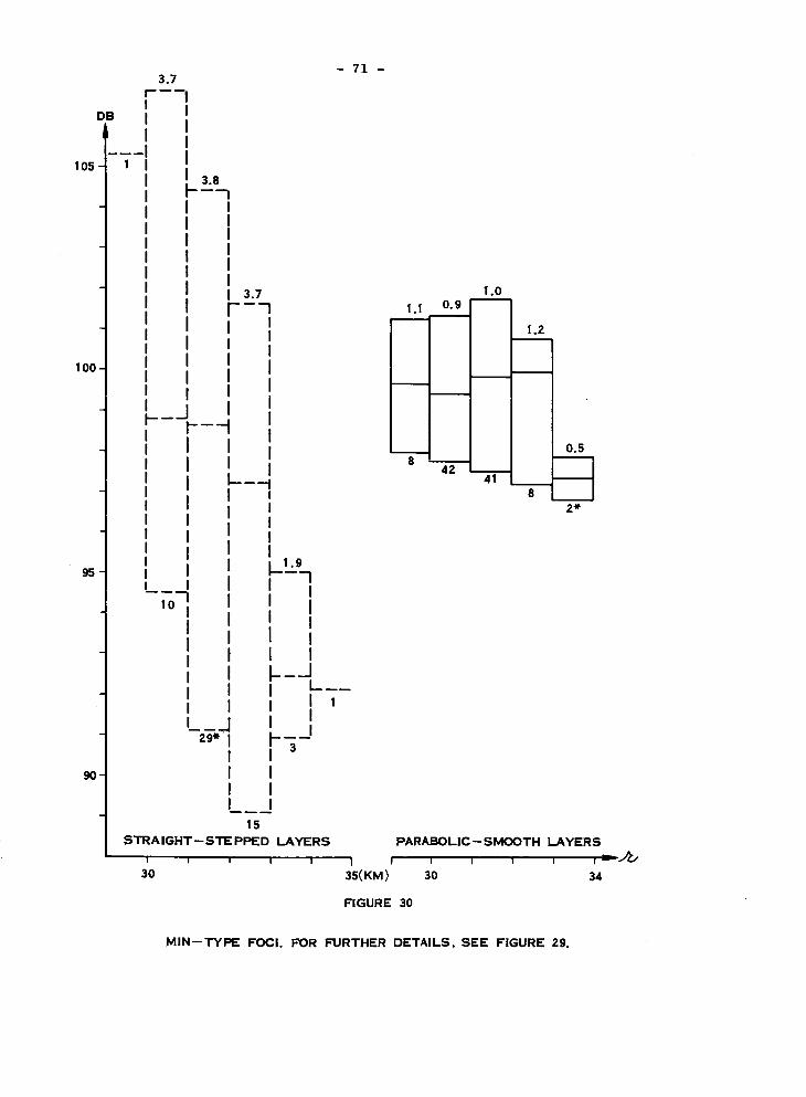
3.7

r------ II I

OB I II I

---I I105 1

100

- "71 -

3.8

3.7

II

IIIIII

lo IIIIIII

I 29.Ji

IIII

15

I_.1 .__9

, I,t II II tI tI---JI L___I II Ii-.__tI 3III

1.1 0.9

I

!

41

1.0

2*

STRA IGHT-- STE PPED LAYERS PARABOLIC-- SMOOTH LAYERS

I I I I I I ! t I I f I _-J'_

30 35(KM) 30 34

FIGURE 30

MIN--TYPE FOCl. FOR FURTHER DETAILS, SEE FIGURE 29.

- 72 -

As to the matter of extent, the parabolic set of

bars covers less radial distance and with less change

in focal intensity than does the linear set. The

parabolic one varies over a 9-km. range; the linear,

over ll km. The parabolic one varies between 77.4-

and 97.4 DB; while, the linear one, between 69.0- and

105.2 DB.

So, in the case of the next-nearest max-type focus,

the differences between the linear and parabolic methods

are indeed very striking. Similar and equally pronounced

differences are found in connection with the next-nearest,

min-type focus; viz., Fig. 30.

In Fig. 30, which is formated like Figs. 28 and 29,

the set of parabolic bars is smaller both DB- and km.-

wise than is the group of linear bars. In terms of

variability, the standard deviation of focal intensity is

less, etc. -- Incidentally, numbers 29 and 2 are starred

to indicate that of these number of loci some occurred more

than once within the specified one-km, interval for a given

atmospheric state. For example, in 26 different atmospheric

states, 29 min-type loci fell in the 31-32 km. interval.

The starred value of 40 in Fig. 28 also has such a meaning

applied to it.

With this introduction of some numbers-of-foal, the

discussion might continue with a few more vital statistics

about loci.

For a sequence of perturbations of the atmosphere

represented by both linear and parabolic layers, the dif-

ferences between these representations is compared in

Table VI (p. 172) in terms of their respective identifi-

cation of the same loci.

- 73 -

Typed between columns two and three of this table is

a product expression. For the atmospheric case listedin column one, and the focal type listed in columnfour, the first factor of this product lists the numberof foci identified by the linear method; the second

factor, by the parabolic one. For example, in Case 4,the linear method identified three min-type loci; theparabolic method, two. In case 4, the linear method

identified two max-type loci; the parabolic method,one. According to column two, all three of the min-typefoal identified by the linear model were within a half

kilometer of one or the other, two min-type loci identifiedby the parabolic method. The value in per-cent listed in

column three is the result of dividing this number 3 bythis product; viz., 0.50 = 3/(3x2).

In the sample of a hundred perturbed atmospheres,

the linear method identified 131 min-type foal; the para-

bolic method, 206. Of these, 69 were within a half kilo-

meter of one another; i.e., a linear (min-type) focus was

within a half kilometer of a parabolic focus 69 different

times. The linear method identified 135 max-type foci;

the parabolic method, 99. Of these, only once did a

linear focus come within a half kilometer of a parabolic

focus.

The value of one-half kilometer was an arbitrary

selection. It turns out that the value 0.86 km. would

have included an additional 53 pairs of min-type loci and

excluded only 17. Here, the pairing is done within the

regime of the nearest, min-type focus or of the next-

nearest min-type. Within either of these regimes, the

largest separation was about 4.5 kilometers (viz., point

A in Fig. 10). In the particular case of the min-type

focus nearest the source, the value 0.63 km. would have

included all pairs, identified by both methods (_. Fig. 2).

- 74 -

1.7 SHORT PERIOD FLUCTUATIONS IN FOCAL DISTANCE

Rays returning to any fixed point is a possibility.

For operational purposes, information about such a prob-

ability would be extremely valuable. In this connection,

focal rays would be of special interest. The likelihood

that a focal ray returns to the same, fixed (focal) point

can be determined by sampling the sound distribution by a

population of randomly fluctuated atmospheric states. In

various ways already, this report has presented this infor-

mation in some of its aspects. Figs. l, 7 and 13, for

example, each show frequency distributions of focal dis-

tance, for the four loci examined in this study. In these

figures, the standard deviations of these distributions are

indicated by the sigma-values printed therein.

The sampled distribution of the closest-in, min-type

foci has a median landing of 7.9 km. and a standard devia-

tion of 279 meters. (This information comes from the para-

bolic distribution of Fig. 1). The sampled distribution of

the closest-in max-type foci has a median landing of S.l km.

with a standard deviation of 286 meters (obtained from the

parabolic distribution inset in the upper-right of Fig. 13).

The next-nearest min-type focus has a median landing of 30.7

km. with a standard deviation of 640 meters (the parabolic

distribution in Fig. 7). Finally, the next-nearest max-type

focus has a median landing of 34.6 km. with a standard

deviation of 1,546 meters (Fig. 13).

The probability of sound returning to a fixed focus is

thus highly variable. According to the above information,

the probability decreases as the distance from the sound

source increases. Namely, focal distance and its standard

deviation increase about linearly at the same rate. The

next-nearest max-type focus, for example, is 4.4 times as

far out as the closest-in min-type focus and has a standard

- 75 -

deviation 5.5 times as great.

The recurrence probability of a fixed focus, moreover, is

exceedingly small. Take for example the next-nearest max-type

focus. If it recurs at all, a third of the time it would recur

more than 1,500 meters apart. And, in this connection, the fact

should be recalled that the spike of focal intensity is but 20-

to 40 meters wide. The result is highly significant, at a fixed

location -- even one known to be in a diagnosed "focal zone" --

the continued threat (for over a fraction of an hour) of any

focally augmented sound at all is very small indeed.

In the last exmmple of the next-nearest max-type focus, its

short-period recurrence probability not as a fixed focus is 92%.

This is fairly high, even though it does range widely. Indeed,

the probability that the max-type focus closest-in would recur

anywhere is only six per cent.

It is evident that numbers-wise, the foregoing examples have

been done with tongue-in-cheek. The distributions in Figs. 1, 7

and 13 show skewness. In view of their shape, it would therefore

appear appropriate to assume their distribution to be, say, a log

normal. Then, the cumulative distribution function could be easily

programmed for the above medians and standard deviations, so as

to provide the selected probabilities that the focal distance

would be less than or equal to radial distance, corresponding to

a specified median and standard deviation. But, in view of the

irregularity in the distributions shown in Figs. 1, 7 and 13,

this was not attempted; for it was felt that normalized treat-

ment of the skewed distributions present ball-park numbers that

tell the story.

Incidentally, the standard deviations expressed parentheti-

cally in Figs. 7 and 13 include all perturbed occasions in which

the focus under consideration occurred; whereas, the other values,

discussed above, do not. Excluded from the latter were all

occasions in each of which more than one such focus occurred. The

reason for preferring the exclusion is obvious. The variability

sought is that due to short-period fluctuations of the atmosphere

as it affects a physically identifiable focus.

CHAPTER II

NUMERICAL ANALYS IS

- 77 -

2.0 THE SOURCE PROGRAM

A case for studying the effects of atmospheric fluc-

tuations and representation upon propagated sound was

presented in the last chapter at some length. Other cases

have been similarly examined. They offered new and con-

vincing evidence reinforcing the conclusion arrived at

in the previous chapter: Namely, as to the limitations

of the straight-stepped representation for diagnosing

the distributed sound-intensity.

These case-studies and their results have been made

available through a specially written program for process-

ing numerical information, h major effort in this.study

was the writing of this program. Called ALLSOND, this

program is presented in this chapter, while the numberical

results obtained by it are tabulated in the concluding

chapter, that follows.

For representing aerological observations, ALLSOND

includes both the linear and non-linear techniques which

were presented by the Program SOUND. This program was

given in KN-67-698-I (pp. 27-54). Mainly, however,

ALLSOND is a numberical technique used for estimating

short-period fluctuations in the noise fields, by means

of an artificial experiment for sampling small-scale

changes in the atmosphere -- the Monte Carlo method.

The resulting estimate yields information as to the

occurrence of small-scale time-induced change in the

noise fields, information as to the likelihood, average

value and variability.

- 78 -

Short period fluctuations in the atmosphere do

affect the distribution of the propagated sound. But,

such changes are not accessible through the routine

observational techniques for sampling the atmosphere.

They could probably not be made available even by the

state-of-the-art observational techniques. Discrete

sampling therefore limits time- and spatial information

about the true turbulent continuum of the sound-propa-

gating atmosphere.

At any place, such changes may be nevertheless

approximated by perturbing the atmosphere in such a way

that the continuum of the small-scale changes so in

reduced is physically compatible with the climatological

experience for that location. ALLSOND applies such a

process to a selection of certain observed initial states

of the atmosphere. A large number of such fluctuated

states of the atmosphere thus approximate the observed

information that would be available from a very dense

array of aerological observations made at very short

intervals of time. From a large number of such short

period fluctuations made of a selected atmospheric condi-

tion, ALLSOND can then obtain the variability of the dis-

tributed sound.

A full run of ALLSOND on the CDC 6400 takes approxi-

mately 17 minutes. This involves one-hundred iterations

of the Monte Carlo method, which is applied to both the

linear and non-linear methods for estimating sound intensity.

In addition, ALLSOND, cranks out a goodly number of statis-

tics about the sound distribution by each method.

Although ALLSOND is detailed as a research program,

- 79 -

still, it also offers a number of new routines possible

for use in the daily operations for predicting varia-

bility of sound propagating. It is therefore felt

advisable to present the program in this chapter, both

for enhancing the better understanding of the results

reported as well as for the possibility of its adaption

to operational use.

Subsequent to the publication of Program SOUND,

recommendations have been received that the program

variables and constants ought to be conveniently defined

in a ready glossary for reference. Accordingly, Section

2.1 alphabetizes the definitions of all variables used

in Program ALLSOND.

In addition to definition, the entries in Section

2.1 also reference other sources in which the defined

variable is discussed or is treated with a mathematical

development. Sometimes, these references present figures

showing some aspect of the defined variable. Such cross-

references are numerous, so as to insure as thorough an

understanding as possible as to the way in which ALLSOND

attempts to execute the general theory, set forth in

earlier publications in this study series.

In addition, the entries in Section 2.1 also specify

the places in ALLSOND where the defined variable is used.

These specifications are given in terms of the routine and

arithmetic-statement number. They may be of some help in

reading the program, especially in seeing how the whole

program fits together.

In Section 2.2, a print-out of ALLSOND is given. As

punched cards, for example, the source program for ALLSOND

- 80 -

is available from the contractor in a limited number.

This source program, incidentally, differs with that of

Program SOUND. ALLSOND is written in the 2.3 Version of

the CDC-6000 Series (FORTRAN 4-D). This ought to explain

the numerous, little differences appearing between SOUND

and ALLSOND, apart from their major differences.

The central problem treated in ALLSOND involves esti-

mation of what percentage of sound emanating from a given

source, after being propagated through an atmosphere under-

going specified processes having known geometry, can be

expected to terminate in certain stipulated locations. If

all relevant probabilities are known for the elementary

events in the life history of such an atmosphere, the Monte

Carlo method is applicable, and indeed is usually the only

method available.

Moreover, its technique is pre-eminently realistic.

It consists in following each of a large number of per-

turbations to the aerological soundings from the basic one

so as to be climatologically consistent both as to point

variation as well as spatial variation along the local

vertical, using the local and spatial elementary probabil-

ities at each data point of the sound. (These are given

by SIGMA CORRI and CORR2 in S INPUT to ALLSOND).

On an aerological sounding of wind- and sound-pro-

pagation speed, a data point is completely characterized

by a set of atmospheric parameters which are climate-wise

sufficient to determine its probable variation in all

situations it may encounter during its history.

The present state of development of high-speed digital

computers permits the use of samples of a size sufficiently

- 81 -

large to ensure satisfactory accuracy in most practical

problems.

The Monte Carlo method of dealing with problems of

this kind breaks up naturally into a well-defined set of

operations. In the Mainline, of ALLSOND, these show up in

arithmetic-statement series 15 to 35+2; 340 to 699 and

1040 through to the end.

It is necessary to have upon call some source of

random numbers equidistributed on the interval 0 __ r <1.

There are computational algorithms adapted to digital

computers which serve this purpose. RANF(X) is the

random number generator used in ALLSOND. (See arithmetic

statements 1065-2 through 1065+1 and the COMMENT therein,

in the Mainline).

In Subroutines FOCI SUM and FOCC SUM, incidentally,

an approximate expression has been used for evaluating the

standard deviation. Thus for the standard deviation, the

sigma values Tables VII (col. 8) and VIII (cols. 8 and 16)

if multiplied by _(n/(n-1)) would provide correct values.

The generally quite small correction would affect slightly

Figs. 23-26, 28-30. For example, in Fig. 23, the point D

would be raised a half a DB; and the point to its left,

about l.l DB. (or about one-half inches on the paper of

Fig. 23). These are the variables SQAX and SQIN in the

glossary given in the next section.

- 82 -

2.1 DEFINITIONS OF VARIABLES AND CONSTANTS

Alphabetizing Definitions of Variables

Used in Program ALLSOND

A (1) Used as a COMMON block name in the mainline

program. (2) Used in Subroutine TENSITY with

constants B and E in order to preserve the

derivative character of landing distance with

respect to the initial ray inclination especially

around data levels in the linear sounding. Here,

A = 1 for ICENT = I; A = -1 for ICENT = I - 1;

A = 1 for ICENT = I + 1. Used finally in arith-

metic statement 488. See p. 34, KN-67-698-1.

AA (I) In the Mainline, AA(LC) = vertex coordinate

of parabola whose arc is fitted to the data points

of atmospheric sounding of the sound-propagation

speed v (in meters per second). Arithmetic state-

ment 699 + I0; see eqn (7), p. 3, KN-67-698-I.

Arithmetic statement 700-4; see eqn 24, p. II,

Ibid. Arithmetic statement 720-4; see eqn (38),

p. 17, Ibid. (2) In Subroutine ADJUST, AA is used

as a counter of the number of angular division into

which a ray-fan is subdivided within any one

refracting layer. Arithmetic statement 130.

(3) In subroutine TENSITY, AA = DXDPHI(I). Arith-

metic statement 488. See DXDPHI.

- 83 -

AAA

AAAI

ABSR

ADD

Used in the Mainline to redefine the parabolic

vertex coordinate of sound-propagation speed when

the sounding half-layers have been resubdivided

at the local maxima. Hence AAA(LC) = AA(L). The

L and LC are respectively the linear data level-

counter and the parabolic level-counter of the

resubdivided half-layers of the atmosphere. Arith-

metic statements 740+6 and 760+1.

In the Mainline, the l'th value of AAA.

The I-index varies between K3 and K2.

K2. Arithmetic statement 851+5.

See AAA.

See KE and

In the Mainline, the value from the library func-

tion ABS(RR). See RR. Arithmetic statement 290-4.

The integrated result of the ray-equation. Com-

putes travel distance of ray penetrating various

types of atmospheric layers in six different ways:

(I) Arithmetic statement 867. For a layer super-

jacent to the minimum of the fitted parabolic sound-

ing-segment for that layer. Comes from Cases I_ and

Ib, p. i14, KN-66-698-1F. Actually, here, only _ or

b need be computed. For example, using the b-expres-

sion for z I in the _-expression listed for Z 1 would

result in reversing the signs of Z 1 and Z 2 and hence

of their sin-l; so that, that result is the b-ex-

pression for Z I. (2) Arithmetic statement 880+1.

For a layer subjacent to a maximum in sounding and

topping out above maximum. From Cases II_ and IIb,

p. 114. Actually, again only _ or b need be computed.

For example, using absolute value of the _-expression

for Z 1 results in the braced expressions for x 2 - x 1

in a and b being reciprocals of one another. Hence,

the absolute value of the log-expression in x 2 - x 1

are the same for both a and b. (3) Arithmetic

- 84 -

ALT

ALTD

ALTM

ALTP

AN

expression 908. For a layer subjacent to a maxi-

mum in a sounding and topping out below that

maximum or at it if K1 = K2 (for which A2 = 1),

but above it if K1 is not equal to K2. From Case

IIa, p. 115, KN-66-698-1F. (4) Arithmetic expres-

sion 920+1. For a ray penetrating a linear layer

above. From Case IVa, p. 115, Ibid. (Incidentally,

there is a typographical error in the IVa-expres-

sion for x 2 - Xl). (5) Arithmetic expression

930+1. For a ray penetrating a linear layer below.

From Case IVb, p. 115, Ibid. (6) Arithmetic expres-

sion 940. For a ray penetrating a linear layer.

From Case IVc.

In the Mainline ALT(NC), where NC varies from 1 to

42, are the altitudes at which statistical matrices

and deviations are given. See NC. Called from

SYMBOLIC INPUT by Arithmetic statement 10.

In Mainline, the difference of ALTP less ALTM. See

ALT, ALTP, ALTM. Arithmetic statement 1091.

In Mainline, "ALT-minus." ALTM = ALT(IM) - ALT(I),

where IM = I-1. The index IM ranges in DO-loop

1095 over the NC-dimensions of the correlation

matrices of temperature (CORR1) and wind (CORR2).

See ALT. Arithmetic statement 1085+3.

In Mainline, "ALT-plus." ALTP = ALT(IP) - ALT(I).

See ALT. IP-- "I-plus," i.e., I+l. ALTP is the

layer thickness superjacent to surfaces at which

statistical matrices and deviations are given.

Arithmetic statement 1085+2.

In Mainline and in the linear model, AN is an accumu-

later-type counter of those requested ranges XI(-),

which (case by perturbation-case) are ensonified.

- 85 -

ANC

ANG

AZ

A1

All

AI2

AAI

A2

B

Arithmetic statement 380-1. See XI and LR. Cf. ANC

Generally, the suffix C indicates that the variable

pertains to operations with the parabolic model.

Hence, ANC is AN in the parabolic atmosphere. See

AN. Arithmetic statement 1380-1.

In the Mainline, "an___ggle." Wind direction in radians,

referred to in its standard position. For example,

a 90 ° -wind = y-wind. Etc.

In the Mainline, the azimuth in radians. In this

study taken as 45 ° .

In the Mainline program, A1 has two meanings. (I)

Parabolic coefficient. Arithmetic statement 899+10.

See eqn (16), p. 7, KN-67-698-I. Arithmetic state-

ment 700-8; see eqn (17), p. 8, KN-67-698-I. Arith-

metic statement 710+3; see eqn (33), p. 15, KN-67-

698-1. (2) Used also as ABS((YYYI-ZZZI)/PI). A1

here corresponds to the Z 1 found on p. 114 of KN-66-

698-IF. See YYYI, ZZZI and P1 in this glossary. Cf.

A2.

In the Mainline program, All = I.+3.E-6.

In the Mainline program, AI2 = I.-I.E-5.

In Subroutine TENSITY, AAI is the focusing factor

according to L.M. Brekhovskikh. Arithmetic state-

ment 630+1. See p. 35c, KN-67-698-I.

In the Mainline program, A2 = ABS((YYYJ-ZZZl)/PI0).

Arithmetic statement 858. Corresponds to Z found

on p. 114 of KN-66-698-1F. See YYYJ, ZZZI _nd Pl.

Cf. AI.

(i) In Subroutine TENSITY B is used with A and E,

to preserve the derivative character of landing

distance with respect to the initial ray inclination,

- 86 -

BDTFAX

BDTFIN

BDXFAX

BDXFIN

B1

CC

CCC

especially around data levels in the linear sound-

ing. B = -i for ICENT = I. B = 1 for ICENT = I - i.

B = 1 for ICENT = I+l. Arithmetic statement 488.

See p. 34, KN-67-698-I. (2) In the Mainline program,

arithmetic statement 1093+1.

In Subroutine PRINT 2, BDTFAX is the biggest dif-

ference in intensity between all pairs of linear and

parabolic foci less than DSTAR apart and of the ma__x

type.

In Subroutine PRINT 2, the biggest difference in

intensity between all pairs of linear and parabolic

foci less than DSTAR apart and of the min type.

In Subroutine PRINT 2, the biggest difference in range

between all pairs of linear and parabolic _oci less

than DSTAR apart and of the max type.

In Subroutine PRINT 2, biggest numerical difference

between all pairs of linear and parabolic _oci less

than DSTAR apart and of the min-type.

In the Mainline, B1 is a parabolic coefficient:

Arithmetic statement 699+8. See eqn (15), p. 6,

KN-67-698-I. Arithmetic statement 700-7: see eqn

(18), p. 8, ibid. Arithmetic statement 700-10: see

eqn (29), p. 13, ibid. Arithmetic statement 710+4;

see eqn (34), p. 15, ibid.

In the Mainline program, the speed of sound from

sounding.

In the Mainline, CC(74) is C for parabolic layers.

Arithmetic statement 730. See eqn (41), p. 18,

KN-67-698-1.

In the Mainline program, CCC(LC) = CC(L). See CC.

Used to redefine the parabolic sound-propagation

speed when the sounding half-layers are resubdivided

- 87 -

CHECK

CI

CM

CORRI

CORR2

CORR3

COSI

COS J

at local maxima. See L and LC, which are respectively

the linear data-level counters and the parabolic level

counters of the resubdivided half-layers of the

atmosphere. Arithmetic statements 740+9 and 760+4.

In the Mainline, initially set equal to O. But there-

after set equal to CORRI(NC, NC) after every square

root of the matrix. Used in Monte Carlo process for

determining whether or not a new correlation matrix

CORRI(NC, NC) has been read in. Arithmetic statement

1047.

In the Mainline program, CI = cos _o" Arithmetic

statement 66+5.

In the Mainline, CM is the mean of sound propagation-

speed for the layer bounded by adjacent levels I and

J, which vary between level 1 (ground) and the top

of the layer in which the ray tops out. Arithmetic

statement 280+1.

In the Mainline, CORRI(50, 50) is the temperature

correlation matrix.

In the Mainline, CORR2(50, 50) are the UEW and the

UNS correlation matrices.

In the Mainline, a vacant correlation matrix.

In the Mainline, the cosine of the angle of inclina-

tion of the phase-normal at level I. Arithmetic

statement 270-5; see eqn (A.13), p. 80, KN-66-698-1F.

The I'th level equals KII, which is an index varying

between the levels 1 and K2, where K2 is the bottom

level of the layer in which the ray tops out. See K2.

In the Mainline, the cosine of the angle of inclina-

- 88 -

COS_

C1

C2

D

DC

tion of the phase-normal at the level J = Kll + l,where Kll is an index varying from level 1 to K2,the bottom level of the layer in which the ray topsout. Arithmetic statement 270.

in the Mainline, the mean cosine function of theinclination through the I-J layer. COSM= (COSI +COSJ)/2. Arithmetic statement 280.

In the Mainline program, C1 has two meanings. (1)As a parabolic coefficient. Arithmetic statement699+7; see eqn (14), p. 5, KN-67-698-1. Arithmeticstatement 700-6; see eqn (19), p. 8, ibid. Arith-metic statement 710+5; see eqn (35), p. 15, ibid.(2) Used also as C1 = COO(I), the I'th value of CCC.

See CCC, K2 and K3, the limits of index I. Arith-

metic statement 855-4.

In the Mainline program, C2 has three meanings. (1)

The J'th value of CCC, where J = I=l. See CCC, K2

and K3, the limits of index I. Arithmetic statement

992. (2) Used also as C2 = CCC(J), the J'th, or

(I=l)'th, value of CCC. See CCC. Also K2 and K3.

Arithmetic statement 855-5. (3) Finally, C2 is

also used for the interpolated value of sound-speed

at the level at which a ray tops out. Arithmetic

statement 992.

(1) In Subroutine TENSITY, arithmetic statement

625+1. See eqn (57), p. 35, KN-67-698-1. (2) In the

Mainline program, arithmetic statement 1093.

In Subroutine TENSITY, DC is the "delta-_hange,"

(x3+ I- Xj_l)/(_j+l- _j_l ), used in the expression

preserving the derivative character of landing distance

with respect to the initial ray inclination. Arith-

metic statement 488-1. See p. 34, KN-67-698-I.

- 89 -

DELX

DEV

DF

DIFF

DM

"Delta-_" in the Mainline program, or the difference

in landing distance between one ray and that of the

"second-previous" ray; viz., the ray whose initial

inclination is two angular increments less than the

first ray. The DELX is employed as a result of the

peculiar way this program earmarks the boundary

surfaces of the atmospheric layers. The PHITOP-ray

of a subjacent layer is the same ray as the PHIBOT-

ray of the next superjacent layer. See arithmetic

statement 1005-2.

De____viation introduced in one of three parameters, in

the Mainline. Deviation introduced in temperature

(K=I), east-west windspeed (K=2), or north-south

windspeed (K=3) at each data level L as the result

of the Monte Carlo process. Arithmetic statement

1094. DEV(L,K) = DEV(37,3).

In the Mainline, the difference in F; i.e., the

sound-propagation speed excess of one level over

that of the subjacent one, Vn+ 1 - v n. Arithmetic

statement 700-11. See F2 and FI. Used in evaluating

the parabolic coefficient C1 for the bottom-half layer.

See eqn (19), p. 8, KN-67-698-I.

In the Mainline, the numerical difference between

VTEST and AAI. See VTEST, AAAI. DIFF is the numerator

of the radicand for the P-function, which is the

vertical distance from the parabolic vertex of a

sounding to the topping-out of the ray for which P

is computed. Arithmetic statement 760+3.

"Delta-minus" in Subroutine TENSITY. Used in preserving

- 90 -

DMTFAX

DMTFIN

DIVLXFAX

DMXFIN

DP

DPH

the derivative character of landing distance with

respect to the initial ray inclination, especially

around data levels in the linear sounding. DM =

(xj - x j+I)/(Vj - _j_l ). Arithmetic statement 482+1g

See p. 34, KN-67-698-1.

In Subroutine PRINT 2, DMTFAX is the means of the

absolute difference in int_ensity between all pairs

of linear and parabolic loci less than DSTAR apartm

and of the max type.

In Subroutine PRINT 2, DMTFIN is the means of them

absolute difference in intensity between all pairs

of linear and parabolic foci, less then DSTAR apart

and of the min type.

In Subroutine PRINT 2, DMXFAX is the mean value of

the difference in range between all pairs of linear

and parabolic loci less than DSTAR apart and of the

max type.

In Subroutine PRINT 2, DMXFIN is the mean value of

of the difference in range between all pairs of

linear and parabolic loci less than DSTAR apart and

of the min type.

In Subroutine TENSITY, "d__elta-plus" is used in preserv-

ing the derivative character of landing distance with

respect to the initial ray inclination, especially

around data levels in the linear sounding. DP =

(xj+ I - xj)/(_j+l - _j). Arithmetic statement 482.

See p. 34, KN-67-698-I.

In Subroutine TENSITY, "d_elta-phi" is PHI1 - PHIO

(where the last suffix is zero). Arithmetic state-

ment 625. See PHI1 and PHIO.

DPHI Called into the Mainline from Subroutine ADJUST.

- 91 -

DPHIC

DPHIMIN

DPHS

DRANM

DRANP

DSTAR

DTFAX

DTFIN

DPHI(255) = increment of PHI.

In the Mainline, DPHIC is the phi-increment in each

refracting half-layer, resubdivided, in the parabolic

model. Called from Subroutine ADJUST by arithmetic

statement 790. Introduced in arithmetic statement

1030.

In the Mainline, the smallest increment for initial

inclination angle.

In Subroutine TENSITY, the DPH-_quared. See DPH.

Arithmetic statement 625.

In the Mainline, the derivative in "Ran-minus."

Arithmetic statement 1090. Used in the Monte Carlo

process.

In the Mainline program, the derivative in "Ran-plus."


Read-in by the Mainline and sent to Subroutine PRINT

2, the ranging-difference criterion (0.5 km.) in

comparing linear and parabolic loci of the same type.

Arithmetic statement i-I.

In Subroutine PRINT 2, the numerical difference inD

_ocal intensity between all possible pair-combina-

tions of linear and parabolic loci of the ma__x-type

which, case for case, are less than DSTAR apart.


In Subroutine PRINT 2, DTFIN(NIN) is the numerical

difference in focal intensity between each member

of all possible pair-combinations of linear and

parabolic foci of the mi__n-type which, perturbation

by perturbation, are less than DSTAR apart. Arith-

metic statment 633-2.

- 92 -

DXPH In Subroutine TENSITY, the first-order

derivative of landing distance with respect

to initial inclination of the I'th ray.

dx/d_o , where _o = PHI(I). Arithmetic

sta + .... + u_-2.

DXDPHI In the Mainline, DXDPHI(255) is the first-

order derivative of landing distance with

respect to initial ray inclination of all

255-rays returned in the linear model.

dx/d_o. Obtained from Subrountine TENSITY

by arithmetic statement 340+2.

DXDPHIC In the Mainline, the first-order derivative

of landing distance with respect to initial

ray inclination of all 255 possible rays

returned in the parabolic model. N.B., in

general, the suffix C indicates that the

suffixed variable pertains to the parabolic

model, dx/d_o. Obtained from Subroutine

TENSITY by arithmetic statement 1040+2.

DXDPHIM In Subroutine TENSITY, the first-order


to initial inclination of the (l-l)'th ray.

dx/_Po , where _o = PHIM. See Figure 14,

p. 35, KN-67-698-I. Arithmetic statement

615+2.

DXDPHIP In Subroutine TENSITY, the first-order


to initial inclination of the (l+l)'th ray.

dx/d_o , where e ° = PHI(IP). In general, the

suffix P stands for "plus." See Figure 14,

p. 35,KN-67-698-I. Arithmetic statement 615+2.

- 93 -

DXDPHI2 In Subroutine TENSITY, the second-order


to the inclination of the (I-l)'th ray.

d2x/d_, where _o = PHIM + PHI(IM). See

Figure 14, p. 35, KN-67-698-I. Arithmetic

statement 633+1.

DXDPHM2 In Subroutine TENSITY, the first-order


to initial inclination of the (I-3)'rd ray.

dx/d_o , where _o = PHI3 = PHI(IM2) = PHI(I-3).

Arithmetic statement 621-2.

DXDPHO (Last character is a zero). In Subroutine

TENSITY, one of two different first-order

derivatives of landing distance with respect

to initial inclination. (The zero suffix

stands for "origin.") One is for the I'th

ray; arithmetic statement 624. See Figure

14, p. 35, KN-67-698-I. The "origin" is

shifted among phi-increments around data

levels in the linear model or levels of re-

subdivision in the parabolic model.

DXF In Subroutine PRINT 2, DXF(-) can be DXF(KIN)

or DXF(KAX). Arithmetic statements 633-7

or 633+1, respectively. It is the numerical

difference in focal distance between each

member of all possible pair-combinations of

linear and parabolic loci of the minimum-type

(KIN) or ma__ximum-type (KAX), respectively,

case-by-case, regardless of how far apart they

are. N.B.:-be sure to recognize the difference

between NIN and KIN, NAX and KAX.

- 94 -

DSFAX In Subroutine PRINT 2, DXFAX(NAX) = DXFK. The

numerical difference in focal distance between

each member of all those possible pair combinations

of linear and parabolic loci of the maximum-type,

case-by-case, which are less than DSTAR apart.


DZ In the Mainline program, height differential.


DZERO In Subroutine TENSITY, the initial intensity in

Decibels, at ground-zero. Arithmetic statement

520-1.

E In Subroutine TENSITY, E is used with A and B,

to preserve the derivative character of landing

distance with respect to the initial ray inclin-

ation, especially around data levels in the

linear sounding. E = 1 for ICENT = I. E = 1

for ICENT = I-1. A = -1 for ICENT = I+l. Used

finally in arithmetic statement 488. See p. 34,

KN-67-698-1.

F In the Mainline, F(255) is the individual focusing

factor = x/(tar_Po dx/dOo), for linear model.

Called from Subroutine TENSITY by arithmetic

statement 340+2.

FC In the Mainline, FC(255) is the focusing factor

for up to 255 different rays in the parabolic

model. In general, the suffix C indicates

that the variable in question pertains to the

parabolic atmosphere. Called from Subroutine


- 95 -

FM In the Mainline, the sound-propagation speed

at level L-1. In FM, M stands for "minus."


FMEAN In the Mainline program, FMEAN is the (weighted)

mean value of F1 and F2 for an atmospheric layer.

For example, arithmetic statements 856, 857, and

992+3. For those layers for which the ray's

incremental travel-distance remains finite, FMEAN

is a reasonably good approximation. In this way,

the integration of F is accomplished; viz., by

the mean of its basic variation with respect to

altitude within a layer.

FP2 In the Mainline program, FP2 = "F-plus 2." The

value of sound-propagation speed at level L+2.

FP2 = V(LP2) = V(L+2). Arithmetic statement 700-14.

FS In the Mainline, the "F-_hear" is the variation

along the local vertical of the horizontal sound-

propagation speed. Arithmetic statement 699+6.

FT In Subroutine TENSITY, FT(255) is, for each landing

ray in the linear model, the total focus factor.


FTC In the Mainline, the total focus factor of the I'th

ray in the parabolic atmosphere. Called from

Subroutine TENSITY by arithmetic statement 1040+2.

FTOTAL In Subroutine TENSITY, FTOTAL accumulates the

value of the focusing factor for each ray returned.

Arithmetic statements 520+3, 520+6, 570, 610.

- 96 -

F1 In the Mainline program,Fl is used to represent

several different types of variables: (I) Sound

propagation speed at the lower boundary of an

atmospheric data layer. F1 = V(L), where (L) is

a data-level index. Arithmetic statement 700-20.

(2) Used also for the value of a certain expres-

sion at the lower boundary of an atmospheric layer.

See eqn (A.47), p. 108 and also p.l13, KN-66-698-1F.

See also eqn (42), p. 20, KN-67-698-I. Arithmetic

statement 855-2. Cf. F2.

FIP' = dVn/dZ . ArithmeticIn the Mainline, FIP is v n n

statement 710-10. See Figure 3, p. 8, KN-67-698-I.

Shear in sound-propagation speed at the lower

boundary of a data slyer. See Figure 9, p. 15,

KN-67-698-I.

F2 In the Mainline, the sound-propagation speed at

the upper boundary of an atmospheric layer.

F2 = V(LP), where the LP index stands for L-_lus;

i.e., the next data level above level L. See

Figure 3, p. 8, and Figure 9, p. 15, KN-67-698-I.

F2 is the value of a certain expression at the

upper boundary of an atmospheric layer. See

eqn (a.47), p. 108. Or, see eqn (42), p. 20,

KN-67-698-I. F2 is a function of altitude, but

does not undergo large changes. Its magnitude

is in the neighborhood of _c/2, neglecting small

effects of U and considering c and ClCOS_Po as

being of the same order of magnitude. Used in

integrating the ray equation for finding the

incremented landing distance of a ray. Arithmetic

statement 855+1. This F-function of a ray for

its topping layer, linear or parabolic, is given

more simply by arithmetic statement 992+1.

- 97 -

F2P " i.e. v' = dVn=i/dZn+ I.In the Mainline, "F2-p_ime, ' n+l

See F2. Arithmetic statement 700-9. Shear in

sound-propagation speed at the upper boundary of

a data layer in the atmosphere. Cf. Figure 9,

p. 15, KN-67-698-I.

GG In the Mainline, GG(LC) is the curvature of

parabolic sounding. Arithmetic statement 699+11;

see eqn (8), p. 3, KN-67-698-I. Arithmetic state-

ment 700-2; see eqn (26), p. ii, ibid. Arithmetic

statements 700+1 and 720+1; see eqn (32), p. 13,

ibid. Arithmetic statement 720-2, see eqn (40),

p. 17, KN-67-698-I.

GGG GGG(LC) = GG(L). See GG. Used to redefine the

parabolic curvature when sounding half-layers

are resubdivided at local maxima. See L and LC;

arithmetic statements 740+8 and 760+3.

GGGI In the Mainline, the I'th value of GGG. See

GGG, K2 and K3, the limits of I.

H H(255) is the height of maximum on the I'th ray.

HC In the Mainline, the height in kilometers of

reference levels in parabolic sounding of the

atmosphere.

I An index frequently used in the Mainline and all

of its subroutines.

IA In Subroutines FOCI SUM and FOCC SUM, IA counts

ma_x-type loci for each perturbation case.

- 98 -

ICENT In Subroutine TENSITY, the arithmetic statements

from 405 through 470 simply restricts the ICENT'th

ray (i.e., the "CENTered" ray) from being either

the PHITOP or PHIBOT ray of an atmospheric layer

or from being the definitional ray ear-marking

the reference levels between layers. See Figure 13,

p. 23, KN-67-698-I.

IDAY In the Mainline program, the date and time,

IE In the Mainline program, the "input-error."

Arithmetic statement I0.

IFL In Subroutine TENSITY. For each perturbation,

the IFL saves the linear-model's focal-count for

its later use in comparing loci between the two

models. Arithmetic statement 630+4.

I FOCU S Found in the Mainline as well as subroutines

TENSITY and PRINT2. The number of focus points

(up to and including eleven) in the linear model.

IFOCUSC In the Mainline, the number of loci in the

parabolic model.

IT In Subroutines PRINT1 and FOCI SUM, FOCC SUM.

(i) Counts min-type loci for each perturbation case.

(2) The row index to the left set and indexes the

arrays for print-out into four sets.

IL In the Mainline, a landing-ray counter. Arithmetic

statements 796, 796+8, etc.

ILM2 In the Mainline, the (IL-2)'th ray. Arithmetic

statement 1005-5.

- 99 -

IM

IM1

IM2

IMAX

IMAXC

IMM

IM2

IN

IN1

IP

Found in the Mainline program and its Subroutines

ADJUST, TENSITY, FOCI SUM, and FOCC SUM. The

index "I-minus;", i.e., I-Io

In Subroutine TENSITY, the index "I-minus-l;"

viz. , 1-2.

In Subroutine TENSITY, the index "I-minus-2;"

viz., I-3.

In the Mainline and its Subroutine ADJUST, IMAX

is the total number of returning rays; viz.,

I-maximum. Applies to the linear atmosphere.

In Subroutine TENSITY, it applies for both the

linear and parabolic atmospheres.

In the mainline, the total number of returning

rays in the parabolic atmosphere.

In the Mainline program, IMM = "l-minus-minus."

IM-I. Arithmetic statement 300 + 2.

In Subroutine Adjust, IM2 = IM, arithmetic

statement 130 + 2.

In Subroutine TENSITY, IN = IMAX -i. IN pertains

to the next but last ray in the fan of returning

rays. Arithmetic statement 613 + 4.

In Subroutine TENSITY, INI = IMAX -2. INI is

the second but last ray in the fan of returning

rays.

Both in the Mainline as well as its Subroutine

TENSITY. IP = "l-plus, '' = I + I. For example,

arithmetic statement 616 in TENSITY.

- I00 -

IRAY Both in the Mainline as well as Subroutine

ADJUST, IRAY(74) = number of rays that bend

in the I'th linear layer.

IRAYC In the Mainline, IRAYC(74) = number of rays

that are bent in the I'th parabolic layer.

IT In the Mainline, IT is an integer-type variable

for certain Hollerith information in the

linear model.

ITC In the Mainline, ITC is an integer-tyep variable

for certain Hollerith information in the parabolic

model.

II In both the Mainline as well as Subroutine

ADJUST, a loop index. For example, Do-loop 160

in ADJUST.

J Used variously an an index and subscript in the

Mainline as well as subroutines ADJUST, TENSITY,

FIT, PRINT1, and PRINT2.

JM In the Mainline, JM is the number of refracting

linear-layers (maxima of v = v + u). In

Subroutine ADJUST, it is the number of refracting

layers of both linear and parabolic layers.

JMC In the Mainline, JMC = the number of refracting

parabolic layers.

Jl In the Mainline, Jl is an index of the 1040-1oop,

over all parabolic, refracting layers.

- I01 -

K In the Mainline, (1) K earmarks a test result;

viz., that the ray is exactly on the layer top

(K = 2) or not (K = 1), in DO-loop 620. K is

also used as a row index to the third set.

(2) Used as an index in Subroutines ADJUST, FIT,

and PRINT1.

KAX In Subroutine PRINT2, for a given perturbation,

KAX is a counter of the same type of max-loci

over all parabolic loci for a given focus I,

where I = I, IFOCUS. See IFOCUS.

KIN In Subroutine PRINT2. For a given perturbation,

KIN is a counter of the same type of min-foci

over all parabolic foci for a given linear focus I,

where I = i, IFOCUS. See IFOCUS.

KMAX In the Mainline and Subroutine ADJUST, KMAX = the

maximum number of rays per linear layer. Called

in the Mainline from SYMBOLLIC INPUT by arith-

metic statement i0. Transferred by arithmetic

statement 60 to ADJUST.

KMAXC In the Mainline, KMAXC = the maximum number of

rays per parabolic layer. From SINPUT. Called

in the Mainline by arithmetic statement i0.

Transferred by arithmetic statement 790 to

Subroutine ADJUST.

KMIN In the Mainline. Minimum number of rays per

linear layer. From SINPUT. Called by arithmetic

statement 10. Transferred by arithmetic state-

ment 60.

- 102 -

KMINC In the Mainline. Minimum number of rays per

parabolic layer. From SINPUT. Called by

arithmetic statement I0. Transferred by

arithmetic statement 790.

K1 In the Mainline. (1) Index to DO-loops 230,

820 and 1000. In the first two DO-loops, K1

references the level of the ray that either

topes out at that level or in the layer sub-

jacent to that level. (Arithmetic statements

210-2, 800-2, respectively.) Used in both the

linear and parabolic models. (2) Also used as

the index to DO-loop 1000 (arithmetic statement 851).

The meaning and values involved in use (1) of K1

have been transferred into the definition of K2,

in turn transferred into the definition of K3,

which retains the original evaluated result

represented by use (1) of K1. Thus, the symbol

K1 has been thereby freed to represent a new

variable; viz., use (2) of K1, which does there-

fore not conflict with use (1) of K1.

KII In the Mainline program, Kll indexes DO-loop 300.

(Here, Kll is an unnecessary replacement for K1,

whose evaluated result has been invested and

retrained into the symbol K2.)

K2 In the Mainline, K2 is used as the upper limit in

DO-loop 300 (arithmetic statement 260+2). The

K2 references the level of the ray that tops out

in the superjacent layer or at its top. Used

as the upper limit in DO-loop 1000 (arithmetic

statement 851). The K2 references the level at

which the PHIBOT-ray (I1 = 1) of a ray-fan tops

out (K = 1), or the bottom of the layer in which

the fan's internal-rays (I1.GT. 1 to I1 .LT. IM-1)

tops out (K = 1), or at the top of which the

- 103 -

PHITOP-ray (I1 = IM-1) tops out (K = 1), or

at the top of which the PHITOP-ray (I1 = IM-1)

tops out (K = 2), except if not only I1 = 1

(and hence K = 1) but also its top is the one

as recognized by the 820-1oop as being above a

local maximum (in which exception the ray tops

out at the level of that maximum). Incidentally,

both bounding levels of this layer are adjacent

LC-levels (viz., either parabolic join-points

at one of the data levels and a mid-level between

them or one such join-point and an LC-subdivision

on a local maximum, over which one parabolic arc

is continuous). Whereas an infinitely ranging

PHITOP-ray asymptotes out always at the top of

the first such layer superjacent to K2, at ex-

tended range the Ii-ray asymptotically approaches

as its zenith a local-maximum level which is

(often well) below the associated K2-1evel. But,

for such an II-ray, the level to be specified

and sought shall nevertheless be that corresponding

to its VTEST-value, contained in the layer mentioned,

since its zenith is otherwise specified by the

height-coordinate of the local maximum. Both K2's

are respectively defined by arithmetic statements

260 and 845.

K2M In the Mainline, K2M = "K2-minus;" viz., K2 - i.


K3 In the Mainline, K3 = I, or K2. Arithmetic

statement 845+3. As the latter, K3 is used as

the lower limit delimiting the 1000-1oop to just

finding the height corresponding to the VTEST-

value of that infinitely traveling ray (viz., the

- 104 -

L

LC

LCOUNT

LCMAX

LLL

LM

PHIBOT ray of the next more elevated fan and

refracting layer to be considered) which tops

out at a local maximum in the sound-propagation

sounding.

In Subroutines PRINT1 and PRINT4, row index to the

3rd set. In the Mainline, a data-level counter.

In the Mainline. In the parabolic model, the

counter of the half-layers resubdivided at local

maxima. See Figure 8, p. 14, KN-67-698-I. Arith-

metic statements 700-23, 740+2 and 760.

In the output Subroutines PRINT1, PRINT2 and

PRINT3, a line-counter.

In the Mainline program, the number of data

levels in the parabolic sounding. Called from

subroutine ADJUST by arithmetic statement 790.

In the Mainline, a control index. For the one-

time calling-up of SINPUT in a lO0-iterated

perturbation of the Mainline by its Monte Carlo

process.

In the Mainline. (i) Number of selected points

XI(-). In LM, L = landing. (2) The number of

levels in the parabolic sounding less one.


LMAX In the Mainline, the number of data levels in

the linear sounding.

- 105 -

LM2 In the Mainline, the index for the second but

last data level in the linear sounding. Arith-

metic statement 699+15.

LP In the Mainline. LP = "!evel-£1us;" viz.,

L = I. Arithmetic statement 750 - 6.

LP2 In the Mainline, LP = "!evel-_lus 2;" viz.,

L = 2. Arithmetic statement 699 + 18.

LR In the Mainline, LR dimensions the array of

requested distances or ranges XI(-). In this

study LR = 40. Called from SYMBOLIC INPUT;

e.g., by arithmetic statements 340+6, 350,

1040+4, 1350, etc.

LT In Subroutine PRINT1, LT = line sub-total for

each model of each perturbation, for which sets

of results are printed four to a row.

M (I) In the Mainline. In a sequence of small-

scale perturbations of the atmosphere, M = the

accumulated number of zero intensity values at

selected points in linear model. Arithmetic

statement 390-3. (2) In Subroutine PRINT3. M(255) =

the number of zero-intensity values at X(-).

MAX In Subroutine PRINT 2. For presentation of cer-

tain Hollerith information. Arithmetic state-

ment 692+1.

MC In the Mainline Program. In Monte Carlo process,

the accumulated number of zero intensity values

at selected points in the parabolic model. Arith-


- 106

MIN In Subroutine PRINT2, for the presentation of

certain Hollerith information. Arithmetic

statement 685+2.

MM In Subroutine PRINT1, PRINT2 and PRINT4. MM =

the upper limit to LCOUNT for paginating and

reheading the title to outputted tables.

Table size for first page.

MP In the Mainline as well as Subroutine PRINT4,

MP = the number of iterations in Monte Carlo.

M = Monte. P = perturbed.

M1 In the Mainline, M1 is the index for DO-loop 112.


M3 In the Mainline, index for DO-loop 117.


N In Subroutine FOCI SUM, FOCC SUM and PRINT4.

N = range of ray's landing distance, in one-

kilometer intervals.

NAME In the Mainline as well as subroutines TENSITY,

PRINT1 and PRINT2. Certain Hollerith informa-

tion identifying linear focal-types. Generated

in Subroutine TENSITY by arithmetic statement

627-9. Called by Mainline at arithmetic state-

ment 340+2 and 1040+2. Inputted into Subroutines

PRINT1 and PRINT2 by arithmetic statement 1045+7

and 1045-1.

- 107 -

NAMEC In the Mainline, certain Hollerith information,

identifying parabolic focal-types. See NAME.

NAMI In Subroutines FOCI SUM and FOCC SUM. NAMI = the

I'th Hollerith value of NAME. See NAME. Arith-


NAP In the Mainline as well as PRINT3. At the requested

ranges XI(L), NAP represents over MP-perturbations

the percent with sound in the linear model.

NAPC In the Mainline program as well as Subroutine

PRINT3. At the requested ranges XI(L), NAPC

represents over MP-perturbations the percent

with sound in the parabolic model.

NAX In Subroutine PRINT2, NAX is a counter of max-

type loci which, model for model, are less than

DSTAR apart.

NAXP In Subroutine PRINT2, NAXP measures the cut-down

effectiveness of DSTAR.

NC In the Mainline program, NC = the dimensions of

correlation matrices. See ALT(42).

NCC In the Mainline, NCC = NC - i.


See NC. Arith-

NFACI In the Mainline as well as subroutines FOCI SUM

and FOCC SUM, NFACI(42) accumulates the n_umber

of m_x-type foci per unit range for all pertur-

bations up through NP.

- 108 -

NFACIC In the Mainline, NFACIC = NFACI for the

parabolic model.

NFICI In the Mainline as well as subroutines FOCI SUM,

FOCC SUM, and PRINT4. NFICI(42) = the accumulated

n_umber of m_n-type loci per unit range for all

perturbations up through NP.

NFICIC In the Mainline, NFICIC = NFICI for the parabolic

model.

NIN In Subroutine PRINT2, NIN is a counter of mi__n_n-type

loci which, model for model, are less than DSTAR

apart.

NINP In Subroutine PRINT2, NINP measures the cut-down

effectiveness of DSTAR.

NNP In Subroutines PRINTI, PRINT2, and PRINT3, NNP

is a page-counter.

NOML In the Mainline as well as subroutines TENSITY

and PRINT2. In general, the L-suffix-ed vari-

ables save information about the linear-model's

loci for their layer use in comparing loci between

the two models. For wxample, IFL, XFL(IFL),

TINFL(IFL), and NOML(IFL). Here, IFL is loci-

count. The NOML(IFL) is the linear focal-type.

(The NOML is a variation upon NAME. See NAME.)


NP In the Mainline program,NP is the Monte Carlo

counter.

- 109 -

NPA In the Mainline and Subroutine PRINT3. At

the requested ranges XI(L), NPA represents

over MP-perturbations the percent without sound

in the linear atmosphere.

NPAC In Subroutine PRINT3. At the requested ranges

XI(L), NPAC represents over MP-perturbations the

percent without sound in the non-linear atmosphere.

NPARI In the Mainline as well as subroutines FOCI SUM

and FOCC SUM, NPARI(42) accumulates the numberm

of ma_x-type cases of £erturbation per each km-

unit of range up through NP cases.

NPARIC In the Mainline program,

the parabolic model.

NPARIC = NPARI for

NPARP In the Mainline and subroutines FOCI SUM and

FOCC SUM, NPARP(N) accumulates £ercent of

NPARI(N) out of MP per each unit range.

NPARPC In the Mainline, NPARPC = NPARP for the

parabolic model.

NPIRI In the Mainline as well as subroutines FOCI SUM,

FOCC SUM and PRINT4, NPIRI(42) accumulates the

n__umber of m_n-type cases of p__erturbation per

each km-un_t of [ange up through NP cases.

NPIRIC In the Mainline, NPIRIC = NPIRI for the parabolic

model.

NPIRP In the Mainline as well as subroutines FOCI SUM,

FOCC SUM and PRINT4, NPIRP(N) accumulates the

percent of NPIRI(N) out of MP per each unit range.

- 110 -

NPIRPC

NPM

NPO

NTEST

NXFAX

NXFAX I

NXFAXM

NXFIN

NXFIN I

NSFINM

In the Mainline, NPIRPC = NPIRP for the parabolic

model.

In Subroutine PRINT3, NPM = "NP-_inus 2"; viz.,

NP - I. (Not used in latest version of Subroutine

PRINT3.

(N.B. - here, the suffix is zero)

1046.

Index to DO-loop

In the Mainline, NTEST provides test routine

alternative. For the parabolic model, NTEST = 0.

Arithmetic statement 50 + I.

In Subroutines FOCI SUM and FOCC SUM, NXFAX

integerizes the distance to max-type foci.

In subroutines FOCI SUM and FOCC SUM, NXFAXI is

the l'th value of NXFAX. Arithmetic statement

645+1.

In Subroutines FOCI SUM and FOCC SUM, NXFAXM =

"NXFAX-_inus," the (l-l)'st value of NXFAX.


In subroutines FOCI SUM and FOCC SUM, NXFIN

integerizes distance to min-type fool.

In subroutines FOCI SUM and FOCC SUM, NXFINI is

the l'th value of NXFIN. Arithmetic statement

660+1.

In subroutines FOCI SUM and FOCC SUM, NXFINM =

"NXFIN-_inus," the (l-l)st value of NXFIN.


- iii -

(No O's.)

P In the Mainline and in Subroutine TENSITY,

certain Hollerith information for the linear

model. Arithmetic statement 340+1 in the Main-

line. In Subroutine TENSITY, P = P or PC,

depending on how the subroutine is called.

PC In the Mainline. A certain Hollerith integer-

type variable for parabolic model. For example,

arithmetic statements 1410+2 and 1046-1.

PERT In the Mainline, PERT(3,50) = storage for

RNDEV(3).

PH In Subroutine TENSITY, PH = PHI(I), the I'th

ray's initial inclination angle. Arithmetic

statement 615+3.

PHI

PHIBOT

In the Mainline, PHI(255) = initial inclination

angle, _o"

In Subroutine ADJUST, PHIBOT is the value of the

initial inclination angle of the bottom ray in a

refracting layer of the atmosphere. Arithmetic

statements 80+3 and 170.

PHIC In the Mainline, PHIC(IL) = PHIZ. Arithmetic

statement 800-4. In the parabolic model, the

initial inclination angle of the IL'th ray.

N.B., in calling Subroutine TENSITY, the Main-

line introduces PHIC for PHI in the Subroutine.


- 112-

PHID In the Mainline program, the value of PHIZ

in degrees, for print-out. Arithmetic

statement 800-8.

PHIM In Subroutine TENSITY, PHIM = "PHI-minus," =

PHI(IM), where IM = I-l. Arithmetic statement

615+1. See Figure 14, p. 35, KN-67-698-I.

PHIM2 In Subroutine TENSITY, PHIM2 = PHI(IM2), where

IM2 = I-3. Arithmetic statement 621-i.

PHIO In Subroutine TENSITY, PHIO is an expression

for PHI(I), where I is the middle data point

of the data triad first above a local sounding

maximum. Defined by arithmetic expression 625+2.

See eqn (58), p. 35b, KN-67-698-I.

PHIP In the Mainline as well as subroutines TENSITY

and PRINT1. In the Mainline, the value in

degrees of PHIO for the linear model. Called

from Subroutine TENSITY by arithmetic statement

340+2. Input-ted to Subroutine PRINT1 by arith-

metic statement 1040-4. See PHIO.

PHIPC In the Mainline, the value in degrees of PHIO

for the parabolic model. Called from Subroutine

TENSITY by arithmetic statement 1040+2. Input-

ted into Subroutine PRINT1 by arithmetic statement

1046. See PHIO, PHIP.

PHIPP In Subroutine TENSITY, PHIPP = "PHI-plus" = PHI(IP),

where IP = I+l. (The double-PP suffix needed to

distinguish this variable from PHIP.)

- 113 -

PHITOP

PHITOPC

In the Mainline as well as Subroutine ADJUST,

PHITOP(20) = _o for the ray that tops at layer

(I = 1, 20). Linear in the Mainline. Linear

or parabolic in Subroutine ADJUST.

In the Mainline program, the value of PHITOP

in the parabolic model. See PHITOP. Called

from Subroutine ADJUST by arithmetic statement 796.

PHIZ

PHIO

PHI1

In the Mainline, PHIZ = "PHI-_ero," an accumulating-

type variable incremented by DPHI(IL) for eval-

uating PHI(IL) and PHIC(IL). Arithmetic statements

66+1, 330, 796+1, 1030.

(Here the suffix-0 is the character zero) In

Subroutine TENSITY, PHIO = PH, Arithmetic state-

ment 623. See Figure 14, p. 35, KN-67-698-1.

In Subroutine TENSITY, PHI1 = PHIM, which is the

"PHI-minus" value, PHIM = PHI(IM). Arithmetic

statement 623. See Figure 14, p. 35, KN-67-698-I.

PSII In the Mainline, PSII is the I'th value of the

tangent-function of the phase-normal. See

eqn (A.II), p. 80, KN-66-698-1F. Arithmetic

statement 280+2. The I varies from 1 to K2.

See K2.

PSIJ In the Mainline, PSIJ is the J'th value of the

tangent-function of the phase-normal. See

eqn (A.II), p. 88, KN-66-698-1F. Arithmetic

statements 280+3, 280+5.

- 114-

PZ In the Mainline and subroutines PRINT2, PRINT3

and PRINT4. Azimuthal value in degrees.

P1 In the Mainline, P1 = the vertical distance from

the parabolic vertex to the topping-out of the

ray for which Pl is computed. See eqn (44), p. 20,

KN-67-698-I, see also p. 114, KN-66-698-I. (The

suffix 1 to Pl here is used as an arbitrary dis-

tinction of this P-function from the other vari-

able P, which is an integer-type variable for

Hollerith information.) Arithmetic statement

851+6. See VTEST, AAAI and GGGI.

Q In the Mainline, a type-integer for certain

Hollerith information in the linear model.


QC In the Mainline, a type-integer for certain

Hollerith information in the parabolic model.


qq In the Mainline, QQ = the value for ZI, p. 115,

KN-66-698-I. Arithmetic statement 910+2.

R Integer-type variable for the presentation of

certain Hollerith information, used in the

Mainline for the linear model. Arithmetic

statement 410+5.

RAN In the Mainline.

and 1080.

See arithmetic statements 1075

RANG In the Mainline and Subroutine PRINT3. RANG(255) =

range of intensity at X(-), in the linear model.

- 115-

RANGC

RC

RNDEV

RR

S

SDTFAX

SDTFIN

SDXFAX

In the Mainline and Subroutine PRINT3. The

range of intensity at X(-) in the parabolic

model.

In the Mainline, type-integer variable for the

presentation of certain Hollerith information in

the parabolic model. Arithmetic statement 1410+7.

In the Mainline, RNDEV(L) = random de____viation of

N(0,1) using N = 16, where the subscript K

indexes temperature (K = i) UEW (K = 2) and

UNS (K = 3). Arithmetic statement 1065+1.

In the Mainline Program as well as Subroutine

ADJUST, RR = the (J'th value of the) PHI-incre-

ment (DPHI) in each refracting layer. Arith-


In the Mainline, S(50,50,3) is equivalenced to

CORRI. Arithmetic statement 1075.

In Subroutine PRINT2, SDTFAX is the smallest

difference in intensity between all pairs ofm

linear and parabolic loci less than DSTAR apart

and of the max type.

In Subroutine PRINT2, SDTFIN is the s_mallest

difference in intensity between all pairs of

linear and parabolic loci less than DSTAR apart

and of the min type.

In Subroutine PRINT2, SDXFAX is the s_mallest

difference in range (XF) between all pairs of

linear and parabolic loci less than DSTAR

apart and of the max type.

- 116 -

SDXFIN In Subroutine PRINT2, SDZFIN is the smallest

difference in range (XF) between all pairs of

linear and parabolic loci less than DSTAR

apart and of the min type.

Tg_S_ In Subroutine T_qSITY, SIG = the sign of

DXDPH. See DXDPH. Arithmetic statement 615+4.

SIGB In Subroutine TENSITY, SIGB = "sign-basic",

the sign of the slope of the r(@o)-Curve at

a previous reference point between which and

the reference point being considered there is

no variation in the sign of the slope.

Arithmetic statements 614-1, 614 and 631.

SIGMA In the Mainline, SIGMA(50,3) = the standard

deviations, 1 = TEMP, 2 = UEW, and 3 _ UNS

for the second index.

sQ In the Mainline, SQ = intensity variance in

the linear model at requested distances.


SQAX In Subroutines FOCI SUM and FOCC SUM, SQAX =2

(TFASQ) See Arithmetic statement 658-2.

sQc In the Mainline, SQC = value of SQ in the

parabolic model. Arithmetic statement 1385+6.

SQIN In Subroutines FOCI SUM and FOCC SUM, SQIN =

(TFISQ) 2. Arithmetic statement 673-2.

T In the Mainline Program, T(37) = temperature

observed.

- 117 -

T_F_ In Subroutine PRINT2, TDTFAX totals the absolute

difference in intensity between the ma__x-type

pairs of linear and parabolic _oci less than

DSTAR apart.

TDTFIN In Subroutine PRINT2, TDTFIN totals the absoluteD

difference in intensity between the mi___-type pairs

of linear and parabolic foci less than DSTAR apart.

TDXFAX In Subroutine PRINT2, TDXFAX accumulates the

numerical difference in range between all pairs

of linear and parabolic foci less than DSTAR

apart and of the max type.

TDXFIN In Subroutine PRINT2, TDXFIN accumulates the

numerical difference in distance between all

pairs of linear and parabolic _oci less than

DSTAR apart and of the min type.

TEMPO In the Mainline, TEMPO(37). The suffix-O =

o__riginal values of TEMP, which are changed from

case to case in the Monte Carlo.

TFAMAX In the Mainline as well as Subroutines FOCI SUM

and FOCC SUM, TFAMAX(N) accumulates the ma___x-value

of intensity of ma_x-type _oci per unit range N

for all perturbations up through NP.

TFAMAXC In the Mainline, TFAMAXC = TFAMAX for the parabolic

model.

TFAMIN In the Mainline as well as subroutines FOCI SUM

and FOCCX SUM, TFAMIN(N) accumulates mi___nn-value

of ma_x-type _oci per unit range N for all pertur-

bations up through NP.

- 118 -

TFAMINC In the Mainline, TFAMINC = TFAMIN for the

parabolic model.

TFASQ In the Mainline as well as subroutines FOCI SUM

and FOCC SUM, TFASQ(N) accumulates the value of

variance SQ of ma_x-type _ocal intensity per each

unit range N for all perturbations up through NP.

TFASQC In the Mainline, TFASQC = TFASQ for the parabolic

model.

TFAX In Subroutines FOCI SUM and FOCC SUM, TFAX(IA) =

TINF(I) = intensity of the max-type loci case by

perturbation-case, where IA is a counter of

max-type loci. Arithmetic statement 635-2.

TFAXI In subroutines FOCI SUM and FOCC SUM, TFAXI(42)

accumulates the value of ma__xx-type _ocal intensity

per each unit range N for all perturbations up

through NP.

TFIMAX In the Mainline as well as FOCI SUM, FOCC SUM and

PRINT4, TFIMAX(N) accumulates max-values of in-

tensity of min-type loci per unit range N for all

perturbations up through NP.

TFIMAXC In the Mainline, TFIMAXC = TFIMAX for the parabolic

model.

TFIMIN In the Mainline as well as Subroutines FOCI SUM,

FOCC SUM and PRINT4, TFIMIN(N) accumulates min-

value of intensity of min-type loci per unit

range N for all perturbations up through NP.

- 119-

TFIMINC In the Mainline, TFIMINC = TFIMIN for parabolic

model.

TFIN In Subroutines FOCI SUM and FOCC SUM, TFIN(II) =

TINF(O) = intensity of mi___nimum-type f_oci over all

perturbations, where II is a counter of m_n-type

loci. Arithmetic statement 635+2.

TFINI In Subroutines FOCI SUM and FOCC SUM, TFINI(N)

accumulates the value of min--type _ocal intensity

per each unit range N for all perturbations up

through NP.

TFISQ In the Mainline program as well as Subroutines

FOCI SUM, FOCC SUM and PRINT4, TFISQ(N) accumulates

the value of variance SQ of mln-type _ocal in-

tensity per each unit range N for all perturbations

up through NP.

TFISQC In the Mainline, TFISQC = TFISQ for parabolic model.

TINF In the Mainline program as well as Subroutines

TENSITY, PRINT1 and PRINT2, TINF(II) = intensity

at a focal point in the linear model.

TINFC In the Mainline, TINFC = TINF in the parabolic

model. Called from Subroutine TENSITY by arithmetic

statement 1040+2. See TINF.

TINFL In the Mainline as well as Subroutines TENSITY and

PRINT2, TINFL saves the linear-model's focal in-

tensities for their later use in comparing loci

between the two models. Arithmetic statement 634-2

in Subroutine TENSITY. Called from TENSITY by

Mainline arithmetic statement 1040+2.

- 120-

TINS In the Mainline, TINS(255) = intensity at landings

of rays; i.e., at ranges of X(-).

TINSO In the Mainline as well as Subroutine FIT, TINSO =

TINS in parabolic model.

TINSM In Subroutine FIT, TINSM = "TINS-minus" = TINS(K-I).


TINX In the Mainline as well as Subroutine FIT, TINX is

the interpolated intensity at requested distances

XI(-). In FIT, arithmetic statements 30, 35, 40

and 45.

TINXC In the Mainline, TINXC = TINX in the parabolic model.

TM In the Mainline program as well as Subroutine

PRINT3. At the requested ranges XI(L), TM(40)

represents over MP-perturbations their mean

sound intensity in the linear atmosphere.

TMAX In the Mainline as well as Subroutine PRINT3. At

the requested ranges XI(L), TMAX(40) represents

over MP-perturbations the ma____ximumsound intensity

in the linear atmosphere.

TMAXC In the Mainline as well as Subroutine PRINT3. At

the requested ranges XI(L), TMAXC(40) represents

over MP-perturbations the maximum sound intensity

in the parabolic atmosphere.

TMC In the Mainline as well as Subroutine PRINT3. At

the requested ranges XI(L), TMC represents over

MP-perturbations their mean sound intensity in the

non-linear atmosphere.

- 121 -

TMFAX In the Mainline as well as Subroutines FOCI

SUM and FOCC SUM, TMFAX(N) accumulates mean

value of max-type f_ocal intensity per each

unit range N for all perturbations up

through NP.

TMFAXC In the Mainline, TMFAXC = TMFAX for the para-

bolic model.

TMFIN In the Mainline as well as Subroutines FOCI

SUM, FOCC SUM and PRINT4, TMFIN(N) accumulates

mean value of mi__nn-type _ocal int__ensity per each

unit range N for all perturbations up through

NP.

TMFINC In the Mainline program, TMFINC = TMFIN for the

parabolic model.

TMIN In the Mainline Program as well as Subroutine

PRINT3. At each of the requested ranges XI(L),

TMIN(LR) represents over MP-perturbations its

minimum sound intensity in the linear atmosphere.

TMINC In the Mainline as well as Subroutine PRINT3.

At each of the requested ranges XI(L), TMINC(LR)

represents over MP-perturbations its minimum

sound intensity in the parabolic atmosphere.

TSQ In the Mainline as well as Subroutine PRINT3,

TSQ(255) = the standard deviation of intensity

at X(-).

TSQI In the Mainline Program, TSQI is numerically the

I'th value of the standard deviation of intensity

at requested distances XI(-).

- 122 -

TSQC In the Mainline as well as Subroutine PRINT3,

TSQC is the value of TSQ in the parabolic model.

TTT In the Mainline Program, the atmospheric temper-

ature at the resubdivided half-layer levels

in the parabolic sounding.

U In the Mainline, U(37) = the wind component

along the azimuth of the ray.

UEW In the Mainline, UEW(37) is the u-component

of sound. U = sound speed. EW = east-west.

UEWO In the Mainline, UEWO(37). The suffix-O =

original values of UEW, which change from

case to case in the Monte Carlo.

UNS In the Mainline, UNS(37) = the v-component of

sound. U = sound speed. NS = north-south.

UNSO In the Mainline, the UNSO(37). The suffix O

stands for the o_riginal values of UNS, the

u-component of wind. The values of UNS are

changed from case to case in the Monte Carlo.

UUU In the Mainline, the aximuthal windspeed at

the resubdivided half-layer levels in the

parabolic atmosphere. Arithmetic statement

775.

Y In the Mainline, V(37) = C(I) + U(I).

- 123 -

VD

VELS

VR

VTEST

VV

VW

In the Mainline, VD is sound-propagation

speed difference between adjacent data levels

K1 and K2 in the linear sounding. K1 refer-

ences the level of the ray that either tops

out at that level or in the layer subjacent

to that level. The K2 references the level

of the ray that tops out in the superjacent

layer or its top; viz., K2 = KI-I. Arith-

metic statement 310.

In the Mainline, VELS = 20.0468. Constant

in evaluating sound speed. See section Ai,

pp. 26 f., KN-66-698-1F.

In Subroutine ADJUST, VR = "V-reference."


In the Mainline. Snell's constant along a

ray. At the zenith of a ray, the sound-

propagation speed by Snell's law.

Co/COS _ + u ° = c/cost0 + u = v o. Used as

a test for V. Arithmetic statement 66+6.

See eqn (43), p. 20, KN-67-698-1.

In the Mainline, VV(74) = V for the parabolic

layers.

In the Mainline, VVV(LC) = VV(L). See VV.

Used to redefine the parabolic coordinate

of sound-propagation speed when the sounding

half-layers are resubdivided at local maxima.

See L and LC, which are respectively the

linear data level-counter and parabolic level-

counter of the resubdivided half-layers of the

atmosphere. Arithmetic statements 740+12 and

760+7.

- 124 -

V1 In the Mainline program, Vl is the I'th

value of VVV. See VW, K2 and KS, the

limits of index I. Arithmetic statements

855-3.

V2 In the Mainline, V2 is the J'th value of

VW, where J = I + I. See WV, K2 and KS,

the limits of index I. Arithmetic state-

ment 855.

WDIR In the Mainline, WDIR(37) is the observed

wind direction.

WSPD In the Mainline, WSPD(37) is the observed

wind speed.

X In the Mainline program, X(255) is the dis-

tance to the grounding of the I'th ray

(I=1,255).

XC In the Mainline, XC(IL) = the parabolic

landing distance of a ray. In general, the

C-suffix stands for parabolic. The index

IL is a ray-counter. In this study IL =

1,255. Arithmetic statement 1005.

XF In Subroutine TENSITY, XF is the f_ocal dis-

tance located from the data triad first above

a local sounding maxima. Defined by arithmetic

statement 626. See equation (59), p. 35b,

KN-67-698-1.

- 125-

XFL In the Mainline as well as Subroutine TENSITY.

For each perturbation, the XFL save the

linear-model's focal-distance (X) for its

later use in comparing loci between the

two models. Arithmetic statement 634-4.

XFLI In Subroutine PRINT2, XFLI is the I'th

value of XFL, where I varies from 1 to IFL.


XFOCUS In the Mainline as well as Subroutines

TENSITY, PRINT1 and PRINT2, XFOCUS(II) is

the distance in kilometers to focal points.

XFOCUSC In the Mainline, XFOCUSC is XFOCUS in the

parabolic model. Called from Subroutine


XI In the Mainline, and Subroutine PRINT3,

XI(40) are the selected points for computing

intensity.

XIO In Subroutine FIT, XIO is the J'th value of

XI(LR), where J varies from 1 to LR = 40, the

number of distances requested. Arithmetic

statement 5-4.

XII In Subroutine TENSITY, XII is the I'th value

of X, the ray-travel distance. (XI not

usable, because XI is SINPUT requested-distance.)


- 126 -

XM In the Mainline and Subroutines TENSITY

and FIT, In the Mainline, XM accumulates

for each ray the landing distance increments

contributed by each resubdivided half-layer

of the parabolic atmosphere, as well as by

the partial topping out layer. For example,

arithmetic statement 950+1. See ADD. Cf. XC.

XM1 In Subroutine TENSITY, XMI = "X-m__inus i" =

X(IMI), where IMI = I - 2. Arithmetic

statement 622-3.

XM2 In the Mainline as well as Subroutine TENSITY,

XM2 = "X-minus 2" = X(IM2), where IM2 = I - 3.

Arithmetic statement 621 - 2.

XO In Subroutine FIT, XO is the K'th value of X.


XP In Subroutine TENSITY, XP = "X-plus" = X(IP),

where IP = I+l. Arithmetic statement 615+1.

XPOCUS In Subroutine TENSITY, XPOCUS(IFOCUS) is the

same as XFOCUS(IFOCUS), except in meters.


XO (N.B.; - the suffix here is zero.) In Sub-

routine TENSITY, XO = Z. Arithmetic statement

623.

Xl In Subroutine TENSITY, Xl - XM.


See XM.

- 127 -

X5 In Subroutine TENSITY, X5 is the numerical

value of X(5) - 5.E3. Arithmetic statement

613+1.

Y In the Mainline, Y(37) = height of data

points.

YTOP In the Mainline, YTOP = "Y-top" the height

in meters at which a ray tops out, between

YYYI and YYYJ. For example, arithmetic

statements 963, 964, 990, etc.

YY In the Mainline, YY(74) = Y for parabolic

layers.

YYY In the Mainline, YYY(LC) = YY(L); See YY.

Used to redefine the parabolic height

coordinate in the sounding of sound-

propagation speed where the sounding half-

layers are resubdivided at local maxima.

See L and LC, which are respectively the

linear data level-counter and the parabolic

level-counter of the resubdivided half-layers.

Arithmetic statements 740+11 and 760+6. See

Fig. 8, p. 14, KN-67-698-I.

YYYI In the Mainline, YYYI - the I'th value of

YYY. See YYY, K2 and K3, the limits for I.


YI In the Mainline, Y1 - the L'th value of YY,

arithmetic statement 750-5.

- 128 -

Y2 In the Mainline, Y2 = the LP'th value of

YY. Arithmetic statement 750-1, where

LP = L = I.

Y3 In the Mainline, Y3 = the L'th value of ZZ.


Z In Subroutine TENSITY, Z = the I'th value

of X, where I varies from 1 to IMAX - i.

ZM In the Mainline, ZM = the LM'th value of Y,

where LM = I - I. Arithmetic statement 700-15.

ZP2 In the Mainline ZP2 = the (L+2)'nd value

of V. Arithmetic statement 700-3.

ZZ In the Mainline, ZZ(LC) = the vertex coordinate

of the parabolic sounding; viz., its height

from sea-level. Arithmetic statement 699+12.

See eqn. 9, p. 3, KN-67-698-I. Arithmetic

statement 700-3; eqn (25), p. ii, KN-67-698-I.

Arithmetic statement 720-3; see eqn. (39),

p. 17, KN-67-698-I.

ZZZ In the Mainline, ZZZ(LC) = ZZ(L). See ZZ.

Used to redefine the parabolic vertex

coordinate of height (measured from sea-level)

when the sounding half-layers are resubdivided

at local maxima. See L and LC, which are

respectively the data linear level-counter

and the parabolic level counter of the resub-

divided half-layers. See Fig. 8, p. 14,

KN-67-698-I. Use as arithmetic statement

740+7 and 760+2.

- 129 -

ZZZI In the Mainline ZZZI is the I'th value of ZZZ.

See ZZZ, K2 and K3, the limits of the index I.


Zl In the Mainline Zl = the L'th value of Y.


Z2 In the Mainline, Z2 = the (L+l)_t value of Y.

See arithmetic statement 700-17.

- 130-

2.2

C

C

CC

C

C

C

C

C

C

PqOGRAM ALLSONO (INPUT, OUTPUT, TAPEMo : INPUT, TAPE'_O)

COMPARISON OF RAY TRACE METNOf15 FOR ESTIMATINC_ 50UNO I_TENSITY VARIATIONSr)UE TO ATMOSPHEOIC VARIABILITY AS DETERMIN_'D BY MONTE CARLO ME'[HODS.

COMMON/A/ AAA (74) ,C (37) ,CC (74) ,CCC (74) ,r)EV (50,p._) _DPNI (255) ,

I OxOPrII(255), F(_55), FT(?55), GG(74), GGr_(74), _(25q), I_L_

?_ IEOCUS, IMAX_, I_AY(Ta), IT9 .IM, M(40), MC(aO), NAME(If), NAP(40).p

3 _IAPC(40)9 NF_CI(42)9 NFICI(4_), NOML(II), NPA(40)_ NPAc(40),4 _PARI(4?)_ NPARP(4_)., NPIRI(,'_.2) ,NPIRP(4__)t D_ °C_

5 oERT(3_,50)_ PHI(P_55), PHIP(I]), _HITOP(20}, _HITOPC(Z_(1), Q_ QC,

6 R, RAN(50), RANG(4(1), RANGC(40}_ RC_ RNDEV(3),p TEMPO(37),

7 TFAMAX(42)0 TFAr,_IN(4_), TFASO(4?)_ TFIMAX(a2), TFIMIN(4?)9

q TF!SQ("2); T!NF(]I), TIN_L(11), TINS(255), TINX(Z_O), TM(40),

0 T_AX(_O), TMAXC(aO), T_C(40), TYFAX(aP), T_RIN(42)_ THIN(40),

I T_INC(_.O), TSQ(40), TSQC(40), TTT(74), UE_(37),_ _IEWO(37),_

3 XFL(II), XFOCUS(II), YY(74), YYY(74), ZZ(/4), ZZZ(7a)

COMMON IOAY(_), Y(37), 7(37), WC)IR(_I), WSof_(37)_ L'_AX, AZ,

i ._PHIMIN,_ KMIN, KMAX, KMINC, KMAXC_, MP, XI("O), LR, SIGMA{50,3),NC_ ALT(42), CORRI(Sn,50), Cc)RP_(50,_O), CoRo3(_O,50)

,]I_ENSION DPHIC(_55), OXDOHIC(_55), FC(25_), _TC(_-_5), H('(25_},II_AYC(74), AA(74), NA_EC(11), AN(40), NFACIC("_), NFICIC(_?),

?_ ANC(40}_ NPARIC(W2), NPAROC(4?),_ NPI_IC(4P), N_RP('(42),

3 OHIC(P-55), PHIPr'(II) , S(SO, 50, "_)• T_At_AxC(4_) _,

4 TFAMINC(42), TFASQC(4__), TFI_,_AXC(42_), T_I._INK(42), TFISF_C(4m),

5 TINFC(II), TIN5_(255), T_NXC(4_), T_AXC(42),

6 TMFINC(42), u(37), XC(?qS) • XFOCUS¢.(II)

EOUIVALENCE (CORRI,S), (D_HI.no_TC) , (L)X_)PHT,f_XOoHIC) _ (c,FC) ,

1 (FT,FTC) , (H_HC) , (!FOCUS,IFOCtI_C) _ (IMAX,IM_XC) , (TRAY,?.RAYC) _,(IT,ITC), (JM, JMC), (NA4E,NA_EC), (PHI,PHIC)_(PHI p,

3 O_IPC), (TIN_,TINFC), (TTN_,TINSC) , (TINX_TINXC) • (wOIR,U), (X,

XC) , (XFC_CUS,XFOCUSC)

DaTA (CHECK : 0,)

TYPE INTEGER O, qC, R, RC, P, PC

LLL = u

S_T UP TEST ROUTINE ALTE_NaTIV_I &"QR THE PARABOLIC _V_On_-L, N " 0 "

READ (60._I) NTERT, qSTAR

I FnRMAT (I II, E6,]}

lh C^LLSINPUT (IE)

SET UP CONTROL 0__ THE POSSIR[_¢ I_oLT-ERR(_;_5.

8 STO0?

6 LLL : I

P_INT 9

9 FORMAT (*0 ERROR IN SINOUT "')

GO TO I07 IF (LLL .EQ. 1) GO TO I0

SET UP ORIGINAL SOUNOT,'_G.

15 Dh 30 I = I, LMAX $ IF (ITFLA_) _r), 2_

20 T(I) = T(1) - 27"_.15

GO TO 3n

_5 T(1) : TEMPO(1)

30 CONTINUE

T_E NP IS MONTE CARLO COUr4TER, ANO NP = I _TAPTS COU_,.iT 0¢ ITERATIONS UP 1"n

_o : I00 _OR THIS STUrOY, FO_ NP : I, SOUNDING lq UNPERTUQHEth.15 4P : I

CLEARS STORAGE FOR CO_RO.

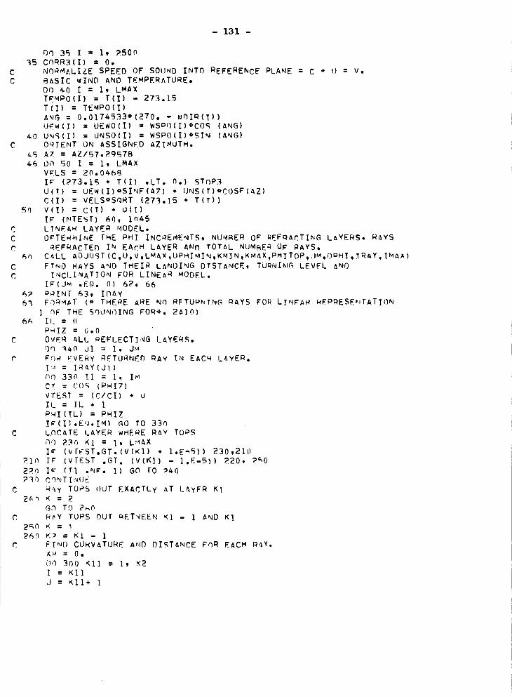
- 131 -

00 35 I = i, ?500

_5 COqR3(1) : O.

C NORMALIZE SPEED OF SOII'_O INTO REFERENCE PLANE : C ÷ U : V.

C BASIC wINO AND TEMPERATURE.

DO 40 I -- i, LMAXTEMPO(1) = T(1) - 273.15

T(I) = TEMPO(1)

ANG = 0.0174533*(270. - whiR(1))U_Tw(1) - UEWO(1) -- wsoi)(1)*CO_ (ANS)

40 U_JS(I} = UNSO(1) = WSPD(1)*SIN (ANS)C O_IENT ON ASSIGNED AZIMUTH.

C5 Al = AZ/ST,_-gST8

46 L)a 50 I = i, LMAX

VI_LS = 20o0468I_" (773",Is + T(i) ,LT, 0,) STOP3

U(T) : UEW(1)*SINF(aZ) ÷ UNS(T)*COSF(AZ)

C(1) - VELS*SQRT (273.15 ÷ T(T))

5n V(1) : C(T) ÷ U(1)

IF (_TEST) 60, In45

C LI_EAH LAYER MODEL,C OETER_INE THE PHI INCmEMENTS, NEJMAER OF nEE_AcTING LAYERS. RAYS

C nEFRACTED IN EAC H LAYER ANn TOTAL NUMBER OF RAYS.An CALL AOJUST (C,U, V, LMAx ,OPHIMIN, KMIN, KMAX,PHI TOP,,IM, OPHI, [RAY, lhAA)

C FT_O HAYS ANO THEIR LANDING DISTANCE, TURNING LEVEL ANDC I,_CI.I_NATION FOR LINEAR MODEL.

I_(J_ .EO. O) 67, 66

62 o_INT 63, IOAY

6"_ FORMAT (* THERE ARE NcI RETUPNIN8 nAYS FOR LINEAR WFPRESE_,TATTON

] 9F THE SqUNC)ING FOR*, 2alO)6f_ IL : 0

P_IZ : 0.0C OVEq ALL REFLECTING LAYERS.

C FF)R EVERY R_TURNEO RAY IN EACH LAYER.I:_I= IRAY(JI)

nO 330 11 = l, I,_

C? = COS (PHIT)

VTEST = (C/CI) ÷ d

If_ : IL + I

P_I(!L) : PHIZ

I:(I].E(_.Ig) GO [0 33n

C LOCATE I.AYER wHErE RAY TOPS

,70 23n KI = I, L'_AXI = (VFFST.GT.(V(KI) ÷ I.E-5)) 230,210

?In I_" (v[EST .GT. (V(K]) - I.E-5}) 220, 2_0

2_0 I_ (_I .N_. I) @0 TO _40

_'_ CONT I_UE

C _,_y TO_5 OUT EXACTLy AT LAyFR KI

GO TO 2_0

C RDY TOPS OUT oET_EEN <I - I AND K1

2_0 K = 1,_6h F,? = KI - I

C F TND CUHVATURE A.IO DI.RTANCE FOR EACH _Y.

_; = O,

Oo 300 Ell : i, K?

I : Kll

J : _II+ I

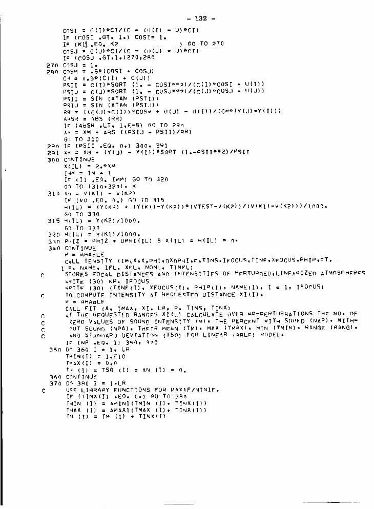
- 132 -

CNSI : C(1)*Cl/(C - (,l(I) - U)*CI)

IF (COSI .GT. l.) C0SI= I°

Ir (KIt,EQ. K?. ) GO TO 270

ChSJ = C(J)*Cl/(C - (O(J) - U)_P,I)I= (c0SJ .GT.I.)270,2Rn

27n C_ISJ - I°__a,_ C_SM : .5"(C0_I + C0S.J)

C_ : U.54'(C(I) ÷ C(J))

PSII = C(1)_*SQRT (I. - COSI**_)/(C(1)*COSI * U(1))

P_IJ = C(J) *SQRT (i. - COSJ*4*_)/(C(J)*COSJ * li(J))

P_II = SIN (ATAN (PSII))

P_IJ = SIN (ATAN (PSI.J))RR = ((C(.J)-C(1))_COS.A + U(J) - LJ(I))/(CM_(Y(J)-Y(1)))

AwSR - ABS (RR)

I¢ (A_$R .LT, I.E-5) r_O TO ?_qqX'4 - XM + ARS ((_SIJ - PSII)/QR)

G0 TO 300

;_Qn IF (PSII .EQ. 0.) 300, 2912QI X_I : XM * (Y(J) - Y(1))*SQRT (I.-_SII**2)/P_;IT

300 C3NT INUEX(IL) = _.*XM

I._M = IM - IIF (11 .EO. I_M) GO TO 320

G_ TO (310,37n), K

310 V._ = V(KI) - V(K;_)

I= (vO .EO, n,) G(} TO "4]5wl(I[.) = (Y(K_) + (Y(KI)-Y(K?))_(VTEST'V(KP))/(V(KI)'V(K2)))/]. 000,

G3 Te 330

315 H(IL) - Y(K2)/1000.

Gq TO 33n3>_0 _(IL) : y(KI)/1000.

3_0 PHIZ -- PHIZ + OPMI(IL) $ X(IL) = H(IL) : n.

3z_0 C_NT INUE= _HA_LE

C_LL TENSITY (IM::X,X_PHI,OXDPHI,It,TINS.IFOCIIS,TINF,XC'OCUS,PHI p,FT, •

I P, NAME, IFL, Xr-L, NOML, TTN_'L)STORES FOCAL DISTANCES ANr_ I_IrE_,SlTl_-S OF PFRTUQRED,I..INF/_nIZED ATMNSPHFR ¢'¢,

wRITE (30) NP, IFOCUS,JnlTFI (30) (TINF(1), XFOCU_;(I), _HIP(1), NAME(1), I : i, IFOCUS)

Tn CO_4PUTE INTENSITY A_T REQtJERTF_ OISTANCE XI(1).

P : _HAmLF

CALL FI[ (X, IMAX, XI, LR, P. TINS_ TINX):T THE _EQUESTED RANGES XI(I.) C#LCULaTE OVE:_ MP-PERTI}RQATTONS TH_ NO. OF

7_ERO VALUES OF SOUND INTENSITY (M), THE PE_C_'NT WITH SOUND (NAP)° WITH-

nOT SOUND (NPA) , THFIR MEAN (TM) , MAX (TMAX) , MTN (TMIN) , RANGE (RANG} ,

_NO 5TAN,)A_) OEVIATTnN (TSn) FOR LI_JEAR (A_LP) MODEl..

I_" (NP .EQo I) 3_(3_ 370

3_N 0 n, 3_0 I = I, LR

T'_IN(1) = I°EIOTMaX(1) = 0.0

T:-_(1) = TS0 (1) = AN (It = 0.3_,0 CONTINUE

370 On 380 I = I,I_R

U_E LI@RARY I:HNCTIONS FOR MAXIF/_IINIF.Ir (TINX(1) .FQ. 0.) r,O TO 3_n

I._IN (1) = AMINI(TMIN (I), TI_X(1))T.,IAX (1) = A,_AXI(TMAX (1), TINX(1))

T_ (I) = TM (1) + TINX(1)

- 133 -

C

C

C

TSQ (I)=TSQ (T) . TINX(1)**?

AN (1) = AN (1) ÷ I.

_R0 CONTINUE

If (NP .NE. MP) GO TO 4]0

Dn 400 I = I, LR

N_P(1) = 100*AN (1)/NP

IF (THIN (1) .EQ. I.EI0) TMIN (1) = 0.IF (AN (1) .EQ. n°) GO TO 390

Tq (1) = TM (1)/aN (1)

SO = l$Q (1)/AN (1) - TM (1)**?

If (SQ .LT. 0.) SQ = 0.

TqQ (I) = SQRT(S{) )RANG (I) = TMAX (T) - TMIN (1)

M (1) : AN (1)

M (I) = MP - M (I)

NPA(I) = 100*M (T)/NPGO TO 400

3QO T_(1) = O,TSQ(1) = 0.

RANG(1) = O,

M(1) = ,_P

NPA(1) = 100,

4n0 CQNTINUE

410 CONTINUECaLL FOCI SUM (NP_ MP, IFOCUS. NAMEr XFOCUS, TIN_, N_IRI, NPARI,

] ',I_IRP, NPARP, N_ICl, NFACI. TMFIN, TMFAX, TFIMIN, TFIMAX, TCAMIN,

TFAMAAt TFISQ_ TFASQ)I; (NP .NE. Mp) GO TO 6_Q

IT = 3HMIN

Q : _HSTRAIGHTR : _d-ST_PPE_S')MMAHIZES OISTRIRUTIQN FOR MTN-TYPE _OCl IN LINEAR ATMOSPHERE.

CnLL PRINT4 (P_ IT_ Q, R, AZ, InAY, MP, NPIQI, NPIRP, NFTCI,TMFIN,

I TFI'41N, TFTMAX, TFISQ)IT : _MAXSOMMaRIZES OISTRIBUTION FOR MAX-TYPE FOCI IN LINEAR ATMOSPHERE.

CALL PMINT_ (P_ IT9 Q, R, AZ, IDAYw _P. NPAql, NDARP. NFACI,TMFAX,

] TFA_IN, TFAMAX, TFASQ)

FnR THE SERIES OF PERTORBED LINEAR ATMS,, OFTERMTNES A_D OUTPUTS THE_ISTRI_UTION OF SOUN_ INTENSITY AT XI(L) = L_ LOCATIONS ALONG ASSIGNE_

AZ(A_LE).C_LL PRINT3 (P_ NP_ MP, AZ, InAY, LR_ Xl, M, NAP_ NPA_ TM_ T_Q,

1 TMIN, TMAX, RANG, MC, NAPC, KIPAC_ TMC, TSQ_, TMINC, T_AXC_ RANGC)

P_QAHOLIC LAYER _0OEL.

A_.JIJSTS LAYERS AND GETS PARABOLA PARAMETERS.

FImST LAYER, TWO POINTS AND ONE TANGENT PARABOLA.

6gg ;1 : V(1)

F_ = V(2)Z_ : Y(I)

Z_ = Y(?)

FmP : (V(3)-V(1))/(Y(_)-Y(1)}

DZ = Z2 - ZlF_ = (F2-FI)/nz

C! : (F2P-FS)/OZ_I : FS*2.*Z2/0Z - F?P*(ZI÷Z2)/_Z

Al : FI ÷ (Z2*E2P-FS*(2*Z2-ZI))*ZI/DZ

.AA (]) = Al - (BI**_)I(_*CI)

_q(1) = CI

- 134 -

Z7(I) :-RI/(2,'0.I)VV(1) : V(1) _, YY(1) : Y(1)

CC (I) = C(I)

L,42 = L,,IAX -

LC : I0(3 740 L. = 2_LM2L m = L * I $ LP2 = I_ ÷ 2 ¢_ I M = L - 1

F1 : V (L)_':_: V(LP}

Z! : Y (L)

Zm = Y (LP)

F_4 : V (LM}

Z.i : Y (LM)F_2 = V(LP2)

ZO2 = y(t.c_2)Ol = Z2 - Zl

DR : F2 - F I

RIP = (I;'2- F_)/(Z2-Z_)

FPP = (FP2-F1)/(ZP2-ZI)

C ROTTOM HALFLaYER,al : Fl

-]1 : FIP*OZ/2.

Cl : (UF-(F_P÷3,*FIP}*I)Z/4,)/_, $ LC : LC ÷ 1

I_'(ARS (Cl/MI},LT,I,E-3) GO Tr} "tno

AA(LC) = al - (BI*'2)/(4,*CI)

Z/(LC) : Zl - 81*DZ/(_.,*CI)6r,(LC) : 4,,Cl/(nZ**2)

Gn TO 710

700 AA(LC) = Al

Gr.(LC) = _**_llOZZZ(LC) = O,

0. THIS ZZ(LC) VALUE FLAr, s LINEA_ ;ORM A ÷ G(Z-Zo), ZO : VALIJE AT

C _OTTOM,

710 CC(LC) = C(L)

YY(LC) = Y(L)

VV(LC) = V(L)

C Tc)P HALF LAYER,

A} = (FI+F2-(F2P-FIP)*F)Z/4,)/_,

_I = OF - (F2P + FIP)oOZ/_.,

Cl = -(UF-(3,oF2P÷FIP)'u'DZ/4.,)/?_,LC = LC * i

If-'(ARS (Cl/RI),LT.I.F-3) GO Tr} 7mn

AA(LC} : A1 - (BI*'2)/(4..*C])ZT(LC) = (Z2+ZI)/2 - RI*F)Z/(4.*CI)

Gr,(LC) = _.,*Cll(c)Z**?)

GQ TO 7307?.0 A_(LC) = Al

Gr_(LC) = 2,'91/DZ

ZZ(LC) = O,730 CC(LC) = (C(L)+C(LP)-((C(LP2)-C(L))/(ZP2-ZL}-(C(I.P)-C(LH))

I / (Z2-ZM) }*DZ/4., )/2

YY(LC} - (Z2÷Zl}/2,

7_.0 VV(LC) = AlLr._AX = LC

C CHECKS FOR MAX WITHIN HALF LAYERS AND RESUdDIVIDF5,

LC = 0

L_ = LCMAX-I

D_ 770 L - i, LM

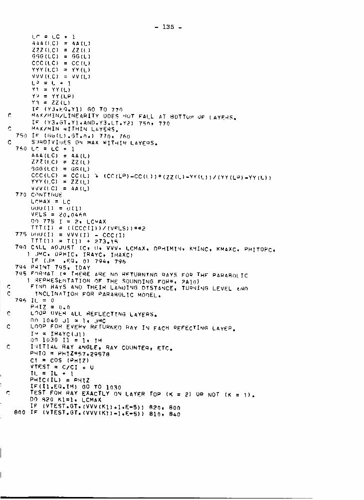
C.

C

C

- 135 -

Lr" = LC * iA&a(l.C) = AA(L)

Z7_Z(LC) = ZZ(L)

GGG(LC) = GG(L)

CCC(LC) = CC(L)

YYY(LC) = YY(L)

VVV(LC) = VV(L)

L_ -.-L ÷ ]

Y1 = YY(L)

Y') = YY(LP)Y_ : ZZ(L)

I¢" (Y3.Eq,YI) GO TO 770M_x/_AIN/LINEARITY OOE_ _quT FALL AT BOTTu._ OV LAYERS.

I_" (Y3,GT,YI,ANO.Y3.LT,Y2) 75n, 770

M_X/_IN _vITHIN LAYERS.

7_() IF (Gb(t.),GT,n,) 7/0, 160

S'JROIVIiJES ON MAX WITHIN LAYERS.

750 Lr = LC ÷ 1

AAA(LC) - AA(L

ZTZ(t.C) = ZZ(L.

_;GG(LC) -- _G(LCCC(LC) - CC(L % (CC(LP)-CC(I.))_(ZZ(L)-YY{I-))/(YY(L_)-YY(L))YYY(I.C) - ZZ(L

vVV(LC) = AA(L770 C(_.NTTNUE

LKMAX = LC

UUU(]) = LI(1)

Dq 775 I = 2, LC_AX

TTT(I) : ((CCC(I))/(V:'LS))_'_2775 U{JU(I) = VVV(I) - CCC(I)

TTT{I_) = T(]) + 273,'1_,?QO C_LL ADJUST (C, t!, VVV, I.CMAX, O_HIMI"_, KHINC, KMAXC, PHITOPC,

] .J_C, L)PHIC, IRAYC, I.-IAXC)

I_ (Jr_ ,EQ, O) 794, 796

794 PQINT 795, 1DAY7q5 FnR'AAT (_, THE_E ARE Nn QFTUPNTNG qAYS FO_ TH_ PAP&@OLIC

] REPARES_r'JTATION OF THE SOUNDING _OR_, PAIO)FTNI3 RAYS AND THEIR LANOING OTSTANCE, TURNING LEVEL _NF)

T_CLINATION FOR PARAQOLIC MOt)EL,

7(}_ IL = 0

P'_IZ = 0o0LOOP OVER ALL REP'LECTING LAYERS.

lqn I0_0 J] = I, J.MCLOOP FOR EVEry RETURNED RAy IN EACH QEFECTING LAYER,

I_ = IRAYC(JI)On 1030 Ii = I, IH

INITIAL RAY ANGLE, RAY COUNTER, ETC.

PHIO = I-}hIZ¢_S7,29578CT ; COS (PHi[Z)

VTEST -- C/CI _ UIL - IL •PHIC(IL) = PH_Z

IF(II,EQ,IM) GO TO 1030TEST FOR RAY EXACTLY ON LAYER TOP (K : 2) (JR NOT (K : l),

DO _20 KI-I, LCMAX

IF (VTEST,GT,(VVV(KI),I,E-5)) 82_, 800

800 I¢ (VTEST,GT,(VVV(K])-I,E-S)) 810, B_O

- 136 -

810 I_ (II._E.I) GO TO _

_PO CnNTINUE

Gq TO RaG_4o K : i

8_5 K_: K1 - I

I; (X_ .EO, _.E5 ,ANn, II ,_0, I) GO TO _50

×'_ : O,

<_ : ]Gn TO 851

C I_OEx DELIMITING THE 1000-|oOm TO JUST FINDING TWE H_IGHT CORRESPONDING ToC THE VTEST-VALUE OF T_AT INFINITELY TRAVELING RAY (ViZ., THE PHI_OT RAY

C OF THE NERT MORE ELEVATED FA_i ANO REFRACTING LAYER HOW TO BE CONSIDERED)

_HICH TOPS OUT _T A LOCAL _AK IN THE SOUND-PROPAGATION SOUNOING.

C LOOP I'0 COMPdTE CURVATUHE A_ID DTSTANCF FOP EACH _AY

8_I nn I000 K1 :K3, K2 \

C KP REFERENCES THE LEVEL AT WHICH THE PHI_OT-RaY (II:]) OF m _AY-FAN TOPS

C OUT (K:I), OR THE BOTTOM Of THE LAYER IN WHICH THE FANS INTERNAL-RAYS (11

C .GT,I TO II.LT.IM-I) TOP OIJT (K:I), OR _T TH_ TOP OF WHICH THE PHITOP-RAY

C (II=IM-I) TOPS OUT (K:2)9 E_KEOT IF NOT ONLY II=I (ANO HFNCE K:I) BUTC ALSO ITS TOP IS THE ()NE AS qECOGNIZED BY THE _20-LOO p AS BEING ABOVE A

C lOCAL MAX (IN WHICH EXCEPTIO_I THK RAY TOPS OUT AT THE LEVEL OF THAT MAX),

INCIOENTALLY, BOTH _OUNDING LEVELS OF THIS LAYFR AQF ADJACENT LC-LEVELS

C (VIZ., EITHER PARAQOLIC JOIN-POINTS AT ONE OF THE DATA LEVELS AND A MID-

C I.EV_L i_ETWEEN THEM OR ONE SUCH JOIN-POINT AND AN LC-SUBDIVISION ON AC LOCAL MAX, OVER WHICH ONE PARABOLIC aPC IS CONTINUOUS). WHFREAS AN INFI-

C _ITELY RANGING PHITOO-RAY ASYMPTOTES OUT ALWAYS AT THE TOP OF THE FIRST

C _UC H LAYER SUPERJACENT TO K_. AT EXTFNOFD PANGE THE If-RAY ASYMPTOTICALLY

r APPROACHES AS ITS ZE_ITH A LOCAL-MAX LEVEL WHICH IS (OFTEN WELL) BELOWC THE ASSOCIATED K2-LEVEL, RUT_ KOR SUCH AN I]-R_Y, THE LEVEL TO aE SPECI-

C ¢IED AND SOUGHT SMALl_ NEVERTHELESS RF TH4 T CORRESPONDING TO ITS VTEST-

C VALUE, CONTAINEq IN THE LAYER MENTIONED, SINCE ITS ZENITH IS OTHERWISE

C SPECIFIEO RY THE MFIGMT-cOORqINATE OF THE LOCAL MAX.

I : KIOGGI : GGG(1)

GGGQRT :SORT (ABS (GGGI))

I_ (GGGQRT ,EO, 0,) GGGQRT : 1.E-TO0

AAAI : AAA(1)P1= SORT (A_S ((VTEST-AAAI)/G_GI))

Z_ZI : ZZZ(1)

0 S_UNT FOR INFINITELY RA._GING oHIqOT-RAY_ TO FIND HEIGHT CORRFSPONDING TO

C TTS ASSOCIATED VTEST VALUE.

IF (XM ,EQ, S,ES ,AND, II .EQ. i) GO TU g60

C ROUND-OFF OF REAL-VARIABLE O-cUNCTION TO FIXED ZERO FOR INFINITFLY RANGING

C _HITOP-RAY.

C ROUND-OFF NOW AUTHORI_ED SINCE LARGEST ROLIN_ ml AT LOCAL _AX .LE, _.77E-?J = I ÷ 1yyYJ = yyy(J)IF (Pl ,LT. 3.E-2 ,AND. GGGI .LT. 0,) GO TO 8R4YYYI = YYY(I)A1 = A8S ((YYYI-ZZZI)/Pl)C_ : CCC(J)

Cl : CCC(1)

V_ = VVV(1)

F1 = (CI*,2 * (Vl-Cl)*(VTEST-VI÷CI))/(CI*SQRT (VTEST÷2,*cI-VI))

IF(KI,NE,K2) RS5, 960

C K! NOT UP TO THE REFERENCE SURFACE FdR WHICH IHE RAy TOPS OUT IN

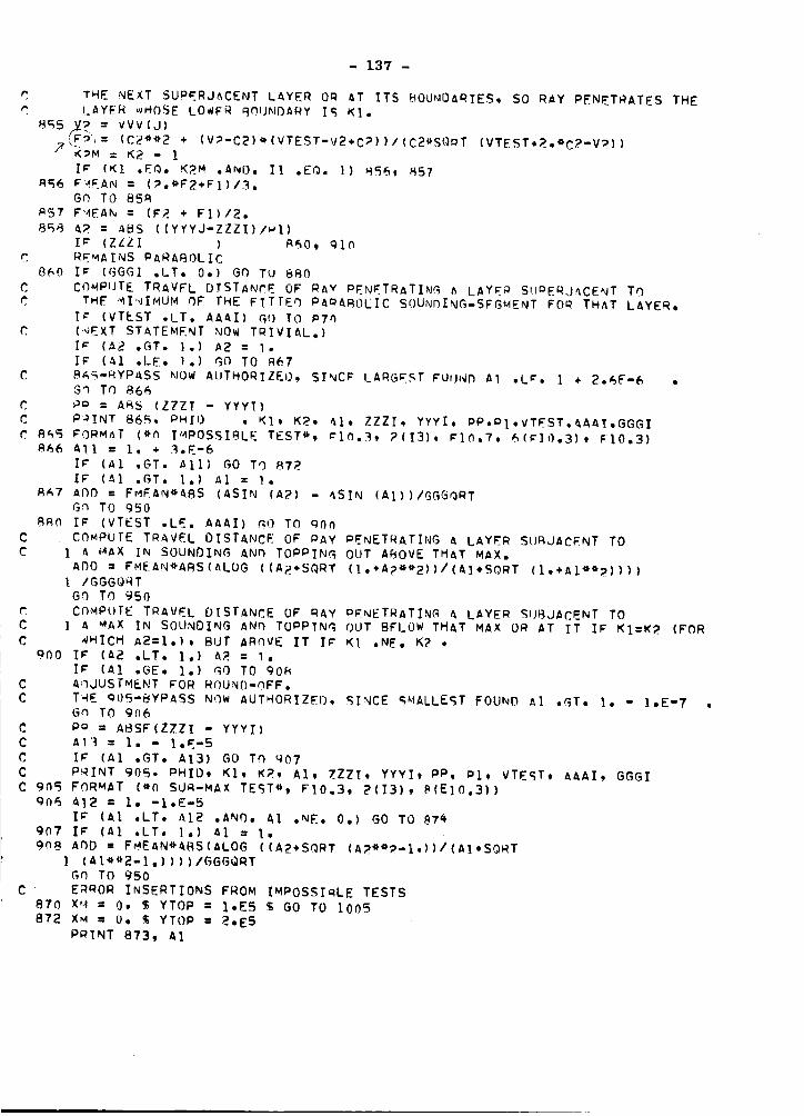
- 137 -

THE NEXT SUP_RJACENT LAYER OQ &T ITS BOUNOARIES, SO RAY PENETRATES THEI AYER wHOSE LO_FR QOUNOARY IS KI.

8_5_ = VVV(J)

_.= (C2"'2 * (V?-C2)*(VTEST-V2÷CP))/(C2*SQpT (VTEST*2.*C2-V?))

I_ (KI .EQ. K2M .AND. II .EQ. 1} H56, _57B_6 F_EAN = (_.*F2÷FI)/3.

GN TO 85_

Q57 F'_EAN = (F2 + FI)/2.

8_@ A_ = AB5 ((YYYJ-ZZZI)/wl)

I_ (ZZZI ) Q_O, gln

C RE_AINS PARABOLIC

8_0 Ic (GGGI .LT. 0.) GO TU BBO

C COMPUTE TRAVFL DTSTANCE OF RAY PENETRATIN_ a LAYER SH_ERJACENT TO

THE ._I'_IMUM OF THE FITTEQ PAoABOLIC S()UN_ING-SEGNENT FO_ THAT LAYER.T_ (VTEST .LT. AAAI) GO TO _7n

C (._EXT STATEMENT _Ow T_IVIAL.}

I_ (A_ .GT. 1.) A2 = I.

I_ (al .LE. I.) GO TO Q_7

C B_-QYPASS NOW AUTHORIZEO, SINC_ LARGEST FU_}Nn Al .LC. i ÷ 2.6E-6 .G_ To 86_

C P_ = AH5 (ZZZI - YYYI)

C P_INT 865. PMIO . KI, K2. _I. ZZZI. YYYI. PP.PI.VTEST.IAAI.GGGI

Q_S FORMAT (*_ IMPOSSIBLE TEST*, _i_.3, ?(13). _I_.7, 6(_10.3), FI0.3)_66 All = I. ÷ 3.E-6

I_ (A1 .GT. At1} GO TO 872

IF (Al .GT. I.} Al = I.

R_7 ADO = FMEAN*ABS (ASIN (A2) - _SIN (AI))/GG_QRTGh TO gSO

8Qn I_ (VTEST .LE. AAAI) GO TO QOn

C COMPUTE TRAVEL DISTANCE OF PAY PENETRATING A LAYER SUBJACENT TOC I A MAX IN SOUNDING ANh TOPPING OUT AQOVE THAT MAX.

ADO = FMEAN*ABS(ALOG ((A2_SQRT (I.÷Ap**2))/(A]÷SORT (1.÷Al**_})))I /GGGQRT

GO TO 950

COMPUTE TRAVEL D[S_ANCE OF RAY PENETRATIN_ A LAYER SUBJACENT TO

C ] A MAX IN SOUNDING AN_ TOPRIN_ OUT BELOW THAT MAX OR AT IT IF KI:K_ (FORC WHICH A2:l.). BU_ ABOVE IT I_ KI .NE. K? •

QO0 IF (a2 .LT. I.) A_ = I.

IF (Al .GE. i.) GO TO 90_C A_JUSTMENT FOR ROUND-OFF.

C THE aOS-BYPASS NOW AUTHORIZFI). SINCE SMALLEST FOUND Al .GT. l. - I.E-7 .Gn TO gn6

C PQ : ABSF(ZZZI - YYYI)C A!_ = i. - I.E-5

C IF (Al .GT. A13) GO Tq gOT

C PRINT g05. PHID. Kl. K_. Al, !ZZl. YYYI_ PP. PI_ VTEST, AAAI, GGGI

C g_S FORMAT (*0 SUP-MAX TEST*_ FIO.3, 2(13), B(EIO.3))gO6 A]2 : l. -I*E'5

I_ (Al .LT. A12 .AND. Al .NE. 0.) GO TO 87_

gn7 I_ (al .LT. l.) al = I.

QNB AOD= FdEAN*ABS(ALOG ((A2+SQRT (A?**_-I.))/(AI+SORTI (AI**2-1.))))/GGGQRT

G_ TO 950

C ERROR INSERTIONS FROM IMPOSSIQLE TESTS

B70 Xq = O, $ YTOP : 1,ES $ GO TO lOOS872 XM = U, $ YTOP = 2,ES

PRINT 873, Al

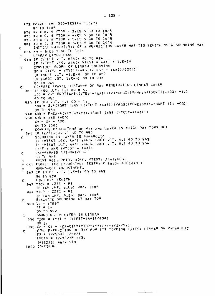
- 138 -

973 FORMAT (*0 200-TEST*, EI0.7)

Gn TO I00_

87_ X_ = O. _ YTOP = 3.E5 $ GO TO lOO_

_75 X_ : O. $ YTOP : 4.E5 $ GO TO 1005

R78 X_ = O. $ YTOP : 5.E5 $ GO TO lOn5

Rfl2 x,_ = O. $ YTOP : 6.ES $ GO TO IOQSC I_ITIAL PHIROT-RaY OF A REFRACTING LAYER HA_ ITS ZENITH OM A _OUNDING MAx

884 X_ : 5.E5 $ GO T_ I00_

C LINEAR LAYER CASF

910 IC (VTEST ,LT° AAAI) _O TO B7AI_ (vTEST ,EQ. AAAl) VTEST : _AAI ÷ I.E-IO

C CnNSIDEH SLOPE OF LINEAR SOHNnINGQQ = (YYYJ - YYYi)/(A_S((VTEST - AAAI)/GGGI))

I; (GGGI .LT. -I.E-8) GO TO g?O

IF (GGGI .GT. l.E-8) GO TO g3n

Gh TO 940C COMPUTE TRAVEL OISTANCE OF _Av PENETRATING LINEAR LAYER

QPn I¢ (QQ .LT; n.) QQ : n.AOO= 2.*(SQRT(A_S((VTEST-AAAI)))/(-GGGI))*FMEAN*(SQRT(I.÷QQ) -i.)

Gh TO 950

930 Ic (QQ .GT. I.) QQ : I.

A_O = 2.*(SQRT (AQS ((VTEST-AAAI)))/GG_}I)*FuEAN*(I.-SQRT (1. -OQ))GO TO 950

940 AO0 = FMEAN*(YYYJ-YYYI)/(SQRT (ARS (VTEST-AAAT))}

9_0 A_O : A_S (ADO)X_ : X_ + ADDGq TO I000

COMPUTE PARA_4ETERS OF way ANO LAYER IN WHICW RAY TOP_ OUT

96o IF (ZZZI.EQ._.) GO TO Q90

K SQUNDING IN LAYER IS PARAROLIK

I¢ (VTEST .GE. AAAI ._ND. GGG? .GT. 0.) GO TO 9&3

IF (VTEST .LF. AAAI .AND. GGG? oLT. 0.) GO TO 96_DTFF = A_S (VTEST - AAAI)

C g_I-QYPASS AUTHORIZED.

Gh TO g@2C P_[NT gGl_ PHTO, ')IFF. VTEST, AAAI,GGGI

C g_1FORQAT (*O IAPOSSIRLE TEST*. m 10.3, _(EIO._))

C ROUND-OFF ADJUSTMENT,gG_ I_ (DIFF .LT. I.E-6) GO TO g63

GO TO 8T_C FIND RAY ZENITH

963 YTOP = ZZZI _ PlIF (XM .NE. 5.E5) g80o 1005

9_ YTOP : ZZZI - Pl

IF (XM .NE. S.ES) 9_0, 1005C EVALUATE SOUNi)ING AT RAY TOP

g_O W = VTEST

A? : I.

Gn TO gg?

C SOUNOING IN LAYE_ IS LINEAR

ggO Y_OP = YYYI + (VTEST-AAAI)/GGql

_I.gq2 C_ = C1 ÷ (C2-Cl}*(YToP-YYYI)/(YYYJ-YYYI)

C FIND F-FUNCTION OF RAY FOR IT_ TOPPING LAYEq. LINEA R oN PARAROLICF? = V2/S_RT (Z'C2)FMEAN : (_,*F_÷FI)/3o

IF(ZZZI) _60, 910

i000 CnNTINUE

- 139 -

IF (XM .EQ. 5.E5 .OR. J1 .GO. i.) GO TO I00_II__2 : IL - 2

XM2 : (XC(ILM2))/_.

Ic (11 .GT. I) GO TO In05

OELX = AH_ (XM - XM2)

IF (DELX .LE. 2.6 } _M : XM2

1005 XC(IL) = 2.*XM

Gn TO (I010, I020), K

1010 HC(IL): YTOP/IO00°GO TO 1o30

I070 HC(II_) : YYYJ/IO00.

In30 PHIZ : PHIZ ÷ DPHIC(IL)

XC(IL) = HC(IL) : 0.0

1040 CONTINUE

PC : _H_RAV_

CALL TENSITY (IMAXC, XC, oMIC. DXnOHIC, FC, TINSC. I:OCUSC,I TINFC, XFOCLISC, PHIPC, FTC, mC, NAMFC, IFL. XFL. NO_L, TINFL)

C TO COMPUTE INTENSITY AT REQUESTE_ DISTANCE XI(I}.

PC : RH_RAVOCALL FIt (XC, IMAXC, XI, LR, oC, TINSC, TINXC)

C AT THE REOUESTED RANGES XI(L) CALCULATE OVEP MP-PERTH_ATIONS THE NO. OF

C 7EHO VALUES OF SOUN_ INTENSITY (M), THE oEoCFNT WIT_ SOll_JO (_AP), WITH-C OUT SOUND (NPA), THFI R _EAN (TM) 9 MAX (TMAX). MIN (TMIN), RA_IGE (SANG),

C _NO STANhARO OEVIATION (TSQ) FO_ PARA_OLTC (mRAVO) _0OEL. AS WELL AS0 MODEL UIFFERENCE.

iF (NP .EQ. l) i350, i3701360 O0 1360 I = I, LR

T_INC(I) = I.EIO

TMAXC(1) = 0.0

TMC(1) : TSQC(1) : ANC(1) : O.13_0 CONTINUE

1370 IC (NP .EQ. MP) GO TO 13@_O0 13_0 I = I, LR

C U_E LIH_ARY FUNCTIONS FOR MaX]F/M!NIF.

I_ (TINXC(I) .EQ. 0.) GO TO I_8nTrAINC(1) = a_IN}(TMINr(1)_ TINXCtT))

T'_aXC(1) = A_IAXI(TMAxc(1). TINXC(1))

T"AC(1) = TMC(1) ÷ TINXC(1)

TRQC(1) = TSQC(I) ÷ T?NXC(1)_2

ANC(1) = ANC(1) • i.13q0 CONTINUE

I_ (NP .NE° MP) GO TO 141013_5 C_NTTNUE

00 1405 I : I, L_

IF (TMINC(I) .EQ. I.EI0) TMINC(I} : O.

NAPC(1) = lOOWANC(1)/_lOIF (4NC(1) .EO. n.) GC} TO 13gn

T'_C(1) = TMC(1)/ANC(1)

Sqc = TSQC(1)/ANC(I) - TMC(1)_pI_ (SQC .LT. 0.) SQC = O.

TSQC(1) = SQRT(SQC)

RANGC(I) = TMAXC(1) - FMINC(1)

MC(I) = ANC(I)MC(1) = MP - MC(1)

NPAC(1) : IO0_MC(1)/NP

GO TO 1_0013_0 TMC(1) = O°

TSQC(1) = O.

- 140 -

R_NGC(1) = n.

Mr'(1) = MP

NPAC(I} = i00

14n0 N_P([] = 100_(AN (1) . A._IC(1)}/NO

NPA(1) = 100_'(M (1) + MC(1))/NP

T_4(1) = TM (1) - TMC(T)

TSQ(I) - TSQ (1) - TSQC(1)

T£QI = A_£(TSQ(1))

I_" (TSLaI .GT. 1000.} TSQ(1) = 0.

TMIN(1) = T_IN (I) - T_41NC(1)

T.,4AX(1) = TMAX (1) - TMAXC(1)

R_NG(I) = RANG ([) - RANGC(1)• i 'r_4([} = ,-,u''(l} '," H_._)

14`o5 CnNTINUE

14,].0 C,')_T I ,'_UE

CALL FOCC SUM (NP, MP, IFOCUSC, NA_4EC, XFOCIISK9 TINF_ NPlRIC.

I r,IPARIC, NPIRPC_. NPARPC, NFICTC, NFACIP, 9 T,'4_'INC, TMFAXCt TFI_41NC,

2 TFIMAXC, TFA_INC, TFAMAXC, T_'ISOC, TFASQC)

IF (NP .NE, MP) GO TO In_.l

Pq : 8HCHARLIE

C FhR TIIE SERIES OF PERTURBED PARARQLIC AT,,4S., DETEQMINES AND OUTPUTS THE

C C_ISTRI_UTION OF SOUND INTENS_rTY AT XI(L) -- Ln LOCATIONS ALONG ASSIGNED

C _Z (HRAVO), AS wELL AS THE CqMPARISON OF TI.4E DI_'FERFNCE _ETWEEN THE

I_INEAR AN}) PARAaOLIC AT_S (CwAPLIE).

CALL PRINT3 (PC.J NP, MP, AZ, TOAY,p LR, XT, M , NAP t NPA , TM 9

I TSQ, T_,IIN, Tr4AX, RANn, _4C, N_OC. NPAC,_ TMC, TSOC, T_._INC, TMAXC,

2 .;ANGC )

=_ = _H_R._VO

qC = HMPARAROLI

He, = HHC-SMOOTH

ITC = 3_tMIN

r StIMMARIZES DISTRIPJUTIqN FOR MTN-TYBE FOCI IN PARABOLIC ATMOSPw'IERE.

CaLL PRINT4` (PC, ITC, (_Ct RCt AZ, IDaY. MPp NPIRIC_ NPTRPtttNFICIC,

I TMFIi'_C, TFTMINC, TFI_4AXC._ T&'TSQC)

ITC : _rIMA_

S_JMM&RI,(ES DISTRIBUTION FOR _IAX-TYPE FQCI I_,_ oARAP_OLIC ATMOSPHERE.

CALL PRINT4` (PC, I/C* QC_. RC, AZ, IOaY. MP_ NC'ARIC._ NPARPC, gNFACIC,

] T_FAXC_. TFAMINC, TFAMAXC,, TFASr_C)

r OFRFQMM MONTE CARLO.

e STORES FOCAL DISTANCES AN[) INTENSITIES OF RFRTURREO OARAr4OLIC AT_,4C)SPHERE£.

10&l WqIT_ (30) NP, IFOCUSC.

_vmTT__. (30) (TINFC(1), xFOCUSC(1), oHIPC(1)_ NAMEc(1), I=I,IFOCUSC,)

IF (NP .EQ. _v1P) GO TO 1045

C Fc_R EVERY PERTUR_AII0_'4 OF _OTN LINEAP AND PARALiOLIC _TMS,,, OUTPUT A COM-

C oARISON OF THE r'_IFFEnENCF BETWEE N THESE AT_4S. IN TEP.MS OF TMEIP #ESPEC-

C TIVE IOENTTFICATION qE THE S_ME EOCI.

C_LL PRINT?_ (AZ, li)AY, NP_. ,MP, IFL_ XFL_ NOML, TTNFL, TINFC,

1 IFOCUSC,,. NAMEC, XFOC!ISC, DSTAR)

1045 NO = .',I_+ 1

I_" (_P .LE. _4P) GO TO 1047

C OUTPUT FOCAL DISTANCES AND INTENSITIES OF PPERTURsED ATMOSPHERES.

RcW INL) 30

Oh 1046 NPo = I, MP

HEA) (30) iMP, IF()CUS

READ (30) (TINF(1)_ X_OCUS(1), PHIP(I}, K_A_F(1), I - 1_ TFOClIS)

P = _rtA_LE

C_LL PRINT1 (P_ NP_ MP, AZ_ It_AY, IE0cUS_ TINF_ XFOCIJS_ PHIP,NAME)

RFAO (30) NP_ [FOCUSC

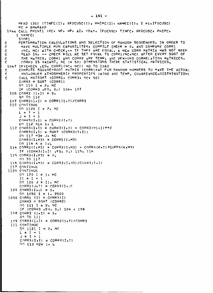
- 141 -

_FAD (30) (TINFC(I), XFOCIJSC(_), _HIPC(I), NAMEC(I), I :I,IFOCIJSC)PC = 8HBRAVO

ln46 CALL PRINT1 (PCt NP_ MP_ AZ_ ?DAY9 IFOCUSC9 T_NFC, XFOCUSCI PHIPCt

1 NAMEC)STriP1

C PERTURBATION CALCULATIONS AND SELECTION OF _ANDOM SEQUENCES, IN ORDER TOC WAVE MULTIPLE RUN CAPASILITES_ COMPILE CHECK = O. ANO COMPARE CORRI

C (NC_ NC) WITH CHECK.-- IF THEy ARE EQUAL. A NEW CORR MATRIX HAS NOT BEEN

C DEAD IN. -- CHECK WILL BE SET EQUAL TO CORPI(NC.NC} AFTER EVERY SORT OF

C THE MATRIX. CORRI ANn CORR2 ARE TEMP. AND VEW-UNS CORREt._TION MATRICES.C CORR3 IS VACANT. NC (: 50) DTMENSIONS THESE STATISTTCAL MATRICES.

10A7 IF(CHEC_ .EQ. CORRI(NC, NC)) _0 TO 1060

C COMPUTE SQUARE-ROOT MATRIX (CnRRI=A) FUR RAHDOM NUMBERS TO HAVE THE ACTUAL

C _ND-ORI)ER ATMOSPHERIC PROPERTIES (wIND ANO TEMP. COvARI&NCE-DISTRIBUTION)

C CALL MATSQRT (CORRI. CORR3, NC, 50)

CORR3 : SORT (CORRI)

Dn 110 I : 2, NC "

IF (CORR3 .EQ. 0.) In_. IO7

lo6 ChRR3 (l,I} : O.

Gn To 110107 CoRR3(I,I) = CORRI(I.T)/CORR3

'^ C,,_ _NUEI&U _ ITT t

Dn 1120 I : _, NC

L : T - IJ = I + I

CnwR3(I.I) = COR_I(I.T)

on 112 MI: I, L11_ CqRR3(I,I) = CURR3(I.I) - COPR3(MI,I)**2

CnRR_(I,I) =SQRT (CO_R3(I,I))

Oq I17 M3= Jr NCCORR3(IoM3) = CORRI(I.M3)

DO 114 _ = I,L114 CORR3(I,M3} = CORR3(I.M3) - COR_(K,T)*COPR_(K_Mg)

IF (CORR3(I.I) .FQ. 0.) 115. _I_

115 CoRR3(I,M3) = 0.aq TO 117

116 C(I_R3(I,M_) = CORR3(I,,A3)/CO_3(T,I)

117 CoNTI_UE1120 CONTINUE

Dh 120 I = I. NCII=I÷1

DO 120 J = If. NC

CORR3(J,I} : CORR_(I,J}

120 CORR3(I.J) : O.

DO 1050 I : I. 2500I0_0 CORRI (I) = CORR,(1)

CORR3 = SORT (CORR2)On III I : 2. NC

IF (CORR3 .EQ. 0.) lOR _ log

lOB CORR3 (I,I) = O.

Ga TO 111

ln9 CORR3(I.I) = CORR2(I.T)/CORRI

111 CONTINUE

on 1121 I = 2, NC

L=I-I

J=I÷l

CqRR3(I,I) = CORP_(I.I)

_ 11.3 _2= I. L

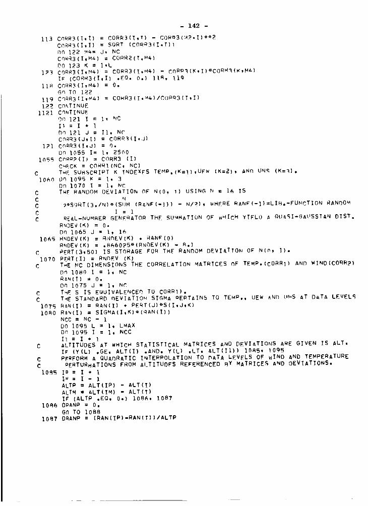
- 142 -

113 CnR_3(I,I) : CORR3(T,T) - COR_3(M?.I)**P.CC_R_3 (I_I} : SORT (COI_'._(I,T))nn 122 M4= Jr NC

Cn_RB(I,M_) : CORR__(I.Ma)

00 123 K = ].Ll_l C-q;_R3(I, ,_) : CORR3(T..M4) - CORP'_(K_I)*CORH'_(K,M_.)

IF (CORR3(I,I) .FQ. 0.) 11_, 11 c)

II_ CnRR3(I_M_) = O.Gn TO I_.2

I19 CqRR3(I,Ma) = COwR3(I.._4)/CORQ3(I,I)

I_- CnNT INUE

II?-i ChNTINUE'_ i"J1 I " I; Mr"J,, &f_ ,_

I1 = I * 1

D r) 121 J = Ii. NC

CnRR3(J_I) : CORRI(I.J)

IP1 Cn_R3(I,J) = O.

Do 1055 I: I, 25n0

1055 Co_P?_(1) = CORR3 (1)

CqECK : CORaI(NC. NC)

C TWE SUHSCRIPT K INDEXFS TEMP.(K=I),UFW (K=2), ANF_ UNR (K:'_).

I060 Oh 1095 K = I. 3

On I070 I : I, NCC T_E RANL)OM DEVIATION (_F N(O_ I) USING N : 16 IS

C NC ?*S.)RT(3./N)*(SIJM (RANF(-])) - N/_), WMEPE RANF(-I)--LIH.-FUNCTION RANDOM

C I = iC REAL-NUMRER GENERATOR THE SUMMATION OF w_Ic H YIFLO A QUASI-GAUSSIA_ DIST.

RNDEV(K) = O.

DO I065 J : I, 161065 RNDEV(K) : R_Mr)EV(K) , RANF(O)

R_IDEV(K) -- .866075* (RNOEV (K) - .q.)

C PERT(3_50) IS STORAGE FOR THE RANDOM DEVIATION OF N(n_ I).

1070 PERT(1) = RNnEV (K)C TWE NC DIMENSIONS THE CORRELATION MATRICES hF TEMP.(cORRI) AND WIND(CORR,)

DQ 1080 I : I, NC

RAN(1) : O.

OC_ 1075 J : i, NCC THE S IS EQUIVALENCEr) TO CORR]).C THE STArbOARD DEVIATIOM SIGMA OEPTAINS TO TEMP., UEW AN[) LINS AT DATA LEVEL_

1075 RAN(1) : RAN(1) • PERT(J}*S(I.J,K)

10._0 RAN(1) : SIGMA(I,K)*(_AN(1))

NCC : NC - I

DO 1095 L = I, LMAXDo 1095 I = I. NCC

II : I ÷ lC ALTITUDES AT WHICH STATISTICAL MATRICES AND DEVIATIONS A_E GIVEN IS ALT,

IF (Y(L) .GE. ALT(1) .AND. Y(L) .LT. ALT(II)) i0_5, 1095

C PERFORM A QUADRATIC INTERPOLATION TO DATA LEVELS OF wIND AND TEMPERATURE

C PERTURBATIONS FROM AI_TITUDES REFERENCED BY MATRICES AND OEVIATIONS.

I0_5 I_ : I ÷ I

I_= I- 1

ALTP = ALT(IP) - ALT(_)

AITM = aLT(IM) - ALT(T)

I_ (ALTP .EQ. 0.) I08_, I087I0_6 OI:ANP : O,

GO TO lOB8I087 DRANP = (RAN(IP)-RAN(1))/ALTP

- 143 -

lOB8 T_ (ALTM .EO, 0,) 10F_o, lOgO

io_9 DOANM -- O,

GO TO i091i0_0 DOANM = (RAN(IM)-RAN(T))/ALTM

IOQI ALTO = ALTP - ALTM

IF (ALTO ,EQ, 0,) 1097, iOg3

1002 rj = n,

H : O,

80 TO 109_1093 O -- (DRANP-DRANM)/ALT_

R = (L)RAr_MeALTP-ORANP"ALT_)/AI T[h1094 OEV(L,K} = RAN(1) + (Y(I.)-ALT(1))_(R*D_(Y(L)-ALT(1)))

1095 C_T I_UE

O0 1096 L = I_ L._AX

T(L) = TF_MPO(L) + DEV(L,I)

U_'w(L) -- LJEWO(L) ÷ DEV(L,?)

U,'JS(L) : UNSO(L} + DEV(L93)

1005 CONTINUE_r_ TO 4(_

E:,!r_

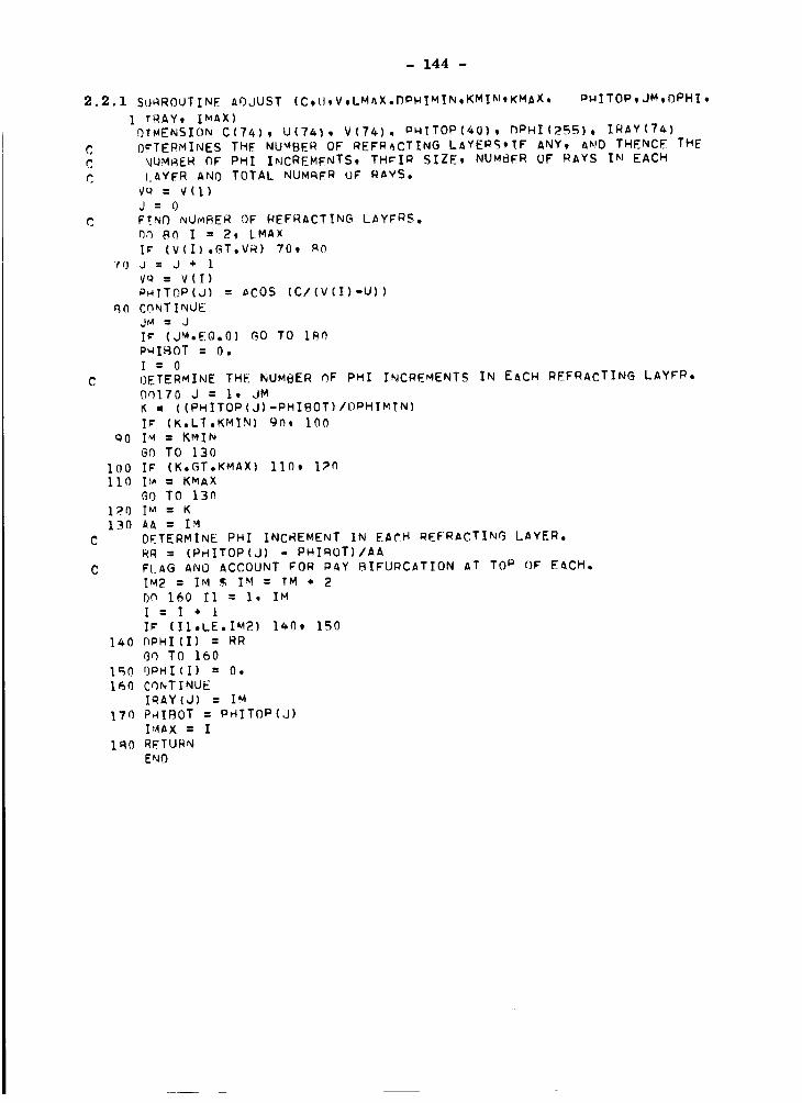
- 144 -

2.2.1 SLJaROUTINE ADJUST (C,U,V,LMAX.r)PHI_IN,KMI_OoKMAX, DwITOp, JM,r)PHI,

I TRAY, IMAX)

DTMENSION C(TA), U(7_), V(74) q OWITOP(40), r_PHI(255), INAY(74)

C O=TERMINES THE NUMBER OF REFRACTING LAYER_S,TF ANY, AND THENCE THE_UM_ER OF PHI INCREMFNTS, THrlP SIZE, NUMSFR OF" RAYS IN EACH

P. I. AYER ANO TOTAL NUMRFR OF RAYS,Vu = V(1)J= 0

C F_Nr) NUMBER OF REFRACTING LAYFRS,r_o 80 I : 2, LMAX

I_" (V(1) ,C_T.VR) 709 _0

70 J - J * i

VQ : V(I)

P_TTOP(J) = =COS (C/(V(I]-U)]

_0 CONTINUE

JM = J

Ir (JM.EO.O) GO TO i_0

P_IBOT = O,

I " 0

C DETERMINE THE NUMBER OF PHI INCREMENTS IN EACH REFRACTING LAYFR.D0170 J = I, JM

K = ((PHITOP(J}-PHIBOT)IOPHI_.TN)

I_" (K,LT.KMIN) 9(Io 100c)O IM = KMIN

GO TO 130100 IF (K.GT.KMAX) 110, l?O

Ii0 I;_ = KMAX

GO To 13o

I_.0 IM = K1.30 AA = I_

C DETERMINE PHI INCREMENT IN EA(_H _EFRACTING LAYER.

RR = (P_ITOP(J) - PHIROT)/AAC FLAG ANO ACCOUNT FOR PAY BIFURCATION AT TOP OF EACH.

IM2 = IM ._ IM = TM ÷ 2

DO 160 11 -" I, IMI = I + I

I_ (II.LE.IM2) 140, 150

140 DPHI (I) = RRGO TO 160

I_0 DRIll(1) = O.

I_0 CONTINUE

IRAY(J} - IM

l?O P_IBOT = PHITOP(J)IMAX = I

I_0 R_'TURNENO

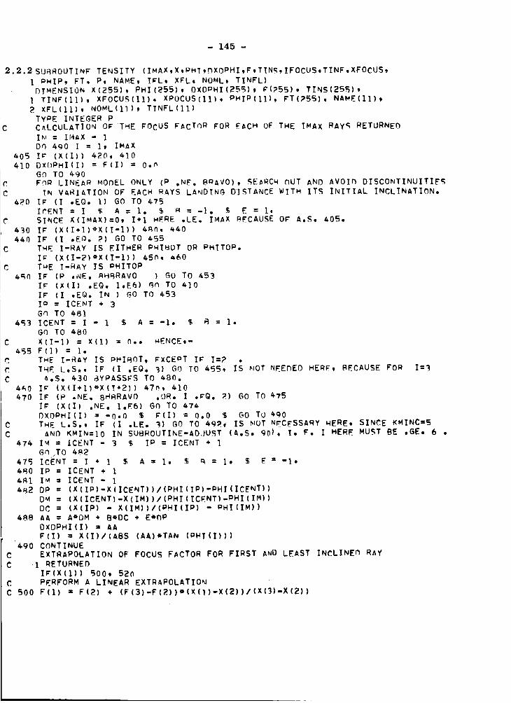
- 145 -

2.2.2 SURROUTINF TENSITY (IMAX�X.PH?.DXDPHI.F.TIN_IFOCUS.TINF.XFOCUS.

I _HIP9 FT. P. NAMEr I_L. XFL. NOMLt TINFL)

DIMENSION X(255). PHI(_5S). DXDPHI(255) t F(_55). TINS(255).

] TINF(II). XFOCUS(I]). XROCUS(II). PHIP(11). FT(?S5). NAME(II)t

2 XFL(II). NOML(I])t TINFL(II)

TYQE INTEGER PCALCULATION OF THE FOCUS FACTnR FOR E_CH OF THE IMAX RAyS RETURNED

I_i = IMAX - IOh 490 I = I. IMAX

_OS I_ (X(1)) 420. 410

410 DX{)PHI(1) = F(1) = O.n

Go TO 490FhR LINEAR MODEL ONLY (P ,NE, BDAVO), SE_RC_ nUT AND AVOIn DISCONTINUITIES

TN VARIATION OF EACH _AYS LANDING DISTANCE WITH ITS INITIAL INCLINATION.

420 I_ (I .EQ. I) GO TO _75

ICENT : I $ A : I. $ _ : -I. $ E : I.

SINCE X(IMAX)=O. I+I HERE .LE. IMAX BECAUSE OF A.S. _05.

430 I_ (X(I÷I)*X(I-I)) 4_n. 4_0440 I_ (I .E_. P) GO TO _5S

THE I-RAY 1S EITHER P_IBOT OR PHITOP.

I_ (X(I-PJ*X(I-I}) 4sn. _0

THE I-RAY IS PHITOP

4_Q I_ (P .HE. _HRRAVO ) GO TO 453

IF (x(I} .EQ. I.E6) _n TO 4}0

IF (I .EQ. IN ) GO TO #53

I_ : ICENT + 3Gn TO 481

4_3 ICENT = I - 1 $ A = -I. $ _ = I.

GO TO 480

C X(I-I) = X(1) = 0.. HENCE.-455 F(1) = I.

T_E I-RAY IS PHIROT. _XCE_T IF I=_THE L.S.. IF (I .EQ. 3} GO TO 455. IS BIOT NEEDED HERF9 BECAUSE FOR 1:3

C _.S. 430 BYPASSES TO 480.

4_0 IF (X(I+I)*X(I+2)) 4In. _I0

470 IF (P .NE. 8HRRAVO .OR. I .rQ. ?) GO TO 475

I_ (X(I) .NE. I.F6) GO TO _7_

DXDRHI(1) = -0.0 _ F(1) = 0.0 $ GO TO #gOC THE L.S.. IF (I .LE. 3) GO TO 49P_ IS _iOT N_CESSARY HERE. SINCE KMINC=_

C AND KMIN=IO IN SUBROUTINE-ADJUST (A.S. 90). I. _. I HERE MUST BE .GE. 6 •

_74 IM = ICENT - 3 $ IP = ICENT + I

Gn_TO 4_475 ICENT = I _ I $ A = I. $ _ = I. $ F = "I"

_RO IP = ICENT + 1

• _I IM = ICENT - I_2 OP : (X(IP)-X(ICENT))/(RHI(IP)-,HI(ICENT})

DM = (X(ICENT)-X(IM))/(RHI(ICENT)-_HI(IM))

OC = (X(IP) - X(IM))/(PHI(I") - _HI(IM))

688 AA = AiOM * BIDC * E*OP

OXOPHI(1) : AA

F(1) = X(1)/(ABS (AA)ITAN (PHI(I}))

_90 CONTINUE

C EXTRAPOLATION OF FOCUS FACTOR FOR FIRST AND LEAST INCLINEn RAY

C I RETURNEDI_(X(1)) 500. 52n

C PERFORM A LINEAR EXTRAPOLATION

C 500 F(1) = F(_) ÷ (F(3)-F(2))I(X(])-X(2))/(X(3)-X(2))

- 146 -

C PFRFORM A QUADRATIC EXTRAPOLATION(A 500-ALT_QNATIVE),

500 F(1)=F(3)÷(X(1)-X(3))_((((F(2)-F(3))/(X(2)-_(3);)_(X(4)-X(3))

I -((F(_)-F(3))/(X(4)-_(3)) )*(x(_}-X(3) ) )/(X(4}-X(2) }+( ((F(_)-F(3))

/(X(4)-X(3) )-( (F(2)-F(3))/(X (2)-X (3}) ) )/(X(4)-X(_) } )*(X (1)-X (3)) )

I= (F(1) ,LE, 0.) 505, 52n

5n5 F(1) = O, $ DXOPHI(]) : O,

5_0 CONTINUE

C INTENSITY CALCULATIONS AT LANDINGS OF RAYS (I, F., AT RANGES OF X(I-))

C HAVING UNIFORMLY INCREMENTED INCLINATIONS

C THE I IS A COUNTER OF LANDING POINTS, UP TO IMAX IN NUMBeR

DZERO : 204,

DO 613 I = I,IMAX

FTOTAL = O,I¢ ( X(1),I_T.I,E-I ,0_, X(?) ,EQ, I,E_) GO TO 60n

Xll = x(I)

FTOTAL = F(1)C FINO 1OTAL FOCUS FACTOR OF RAYS RETURNED TO EACH LANnING

C T_E I,_NER 5RO-LOOP COMPARES THE RANGING OF qAYS RETWCEN EVERY I-POINT ANn

C EVERY JP-LANDING-POI.IT.IN = IMAX - I

DO 5aO J : 19 IN

C AVOIDS THE BOUNDARIES UF T_E QEFRACTING LAYERS

J: : J ÷ I

550 I¢(X(J)*X(JP)) 560, 5aO560 IF((X(J)-XII}*(XII-X(JP)),GT,n,) 570, 580

C CASE I - J ,GT, I, BETWEEN XII AND X(JP) THE RAY-RANGE TPENOS EITHER

C FIRST INWARD TOWARD THE SOUND-SOURCE BUT THEN BACK OUTWAUD PAST XII, IF

C X(JP) IS GREATER THAN XII, On ELSE OUTWARD FROM XlI ANO THEN INWARD AND

C _GAIN PAST Xll Of_ TOWARD THE SOURCE, IF THE JP-_AY LANDS CLOSER TO THE

C SOURCE THAN DOES I-RAY, CASE IT - ,JP ,LF, I. BETWEEN x(J) AND XlI THEC RAY-RAnGE TRENDS EITHER FIRST OUTWARO PAST Xll RUT THEN _ACK TO XII (IF

C x(J) IS LESS THAN XII), OR ELSE INWARD TOWAR_ THE SOURCE BUT THEN BACK

e OUT TO Xll (IF THE LANOI_IG DISTANCE OF _-RAY IS CLO_ER TO THF SOURCE THAN

C THAT OF J-RAY). - BUT, A 570-BYmASS TO 5BO INOICATE_ THAT T_W RAYS ARE

C cONTINUING RELULARLY TO GET EITHER AWAY FROM XII OR CONTINUT_!G TO RANGE

C CLOSER TO XII.

570 FTOTAL = FTOTAL * F(J) ÷ (F(J_}-F(J))"(XII'X(J))/(X(.IP)-X(J))

5_0 CONTINUE

IF (FTOTAL .GT, O, ,AND, XII .GT, I,E-20) 5_0, 600

5gO rI_,S(1) = DZERO -18.370 ÷ 4,3_2Q*ALOG(FTOTAL/(XII"*_))

Gn TO 610

600 TINS(1) = 0.0

610 FT(1) : FTOTAL

I_ (X(1)) 613, 6]._

612 IF (I ,,wE, I) GO TO 6]]FT(1) = I,

613 CONTIi_UE

X_ = ASS (X(5) - 5,E3)

I; (X5 ,LE, I,E2) GO TO 640

C LOCATE FOCI ANO COMPUTE I_tTEN_ITY THERE

I_OCUS = 0

IN : IMAX- I

IN] : IMAX-IF(OXOP_I(1),NE,O,) GO TO 61_

SIGB = SIGN (I,,OXOPHT(_))

Go TO b15614 S?G_ : SIGN (I,,OXOPHI(1))

C FINO NUMBER OF FOCI

- 147 -

C FnR EACH PERTURBATION NP=IpMP, THE KS SURSCRIPT THE LINFaR-MODEI. FOCIS

C PANGE, TyPE AND INTE_SITY ANn SAVE THESE VALUES FOR THEI_ LATER COMPARI-

C qON WITH THOSE OF THE PARABOLIC MODFL,

6]5 DO 632 I = 2,1NIM = I - I $ IP = I , I _ XM = X(IM) _ 7 = X(1) $ XP= X(IP)

OXDPHIM = OXDPHI(IM) _ DXOPH = nXDPMI(1) $ DXDDHI p = _XDPHI(IP)

P_IM = PHI(IM) $ PH = _HI(1) _ P_IPP = P_I(IP)

SIG = SIGN (I,,DXDPH)C FhR AN INFINITELY RAN_ING PHIqOT-RAY,A 63}-QYPASS HERE (INSTEAD OF TO &32)

C MAKES SIGB NEGATIVE (8ECAUSE OF A.S, _70÷21, HENCE THIS RAY WILL NOT BEC CONSIDEREO AS A MAX-FOCUS TH_ NEXT TIME THmOIIGH THE 632 nO-LOOP,

I: (Z ,EQ, l,F6) GO To 631

IF (Z ,EO, 0,) GO TO 632C RaY HAS FINITE RANGE,

IF(SIG,EQ,SIGB) GO _o _32

IF (P ,EQ, 8HBRAVO ) GO TO &l&C LINEAR MODEL _YPASS TO DISREGARD POSSIBLE FALSE FOCUS AT EAC_ DATA LEVEL,

IF (XM ,EQ, O, ,OR, XP ,EQ, 0,) GO TO 631

6]6 IFOCUS = IFOCUS + iC FIND DISTANCE TO A FOCUS,C IN THE PARAROLIC CASE, FOR I:_ TO HAVE GOTTEN TO HERE, XM ,NE, O, AND

C HENCE tHE I=_ BYPASSES TO 8_I,,

!_ (XM ,N E. O..oP, PH .HE, PHIM) GO TO _I

C IN THE PARABOLIC CASE, XM=O CONSTOERS PuSSiRiLiTY THAT F,qCvS FALLS _ETwEEM

C PHIBOT I-RAy AND THE NExT-RuT-LAST PAy OF PRFCEEDING (NEXT I.OW£R) FAN O_

C PAYS, mENCE, FOR (?NO-OROEP) INTERPOLATING THIS FOCAl. DISTANCE (RY A,S,

&26)9 THE LASI PREVIOUS AVAILABLE RAY WITH DIFFERENT LANDING DISTANCE ANn

C VARIATION (DxDPHI) IS THE ONE BEFORE THE PHITOP.RAY OF PREVIOUS RAY-FAN,

C THE L,S,, IF (I ,LE, _) GO TO , IS NOT NECESSARY HERE, SINCE KMINC:_

C ANO KMIN=IO IN SUBROUTINE-ADJUST (A,S, qo), I, E, I HERE MUST BE ,GE, 6 ,

IM2 = I-3 $ XM2 = X(IM2) $ PHTM_ = PHI(IM?} $ DX_PHMR=DXOPHI(IM2)

XM = XM2 $ PHIM = PHIM2 _ DXOPHI_ : OXOPHM2C I_ VICI_'_ITY OF A FOCUR BETWEEN ADJACENT RAYS_ SO COVARY _ANGE AND INCLINA-

C TION T_AT THEY HAVE THE @EST 2NO-ORDER FIT NEAREST THE RAY HAVING THE MOP

C EXTRE:_E RANGE_ wHETHR_ THE LONGEST O_ SHORTEST,

6Pl IF (SIG_ ,GT, 0,) GO TO _22C CONSIDERS THE POSSIBII.ITY Z,GT,XM ATTENOING THE INVALID I_SE OF A OXOPHO=

_3XDPHIf_ B_SED ON XM],EQ,I,F_, A CONDITION TO BE REPLACED BY A QUADRATIC

C INTERPOLATION INVOLVING THE _ OATA-DOINTS CENTERED ON I, THE 2ND A_OVE A

C LOCAL SOUNOING-_AX POINT (_Nn RAY AHOVE PHIBOT HAVING INFINTTE RANGE),

I_"l = I - 2 $ XMI = X(IMI)

IF (XMI ,EQ, I,E_) GO TO _P3

I_ (Z ,LT, XM) 6_3_ 6_

6?2 IF (Z ,LT, XM) GO TO %2_

8P3 Xn = Z $ DXDPHO = _XOPH $Xl : _M $

_?_ X0 = XM _ OXDPHO = _XDPHIM $

×l = Z $6_S O_M = PHIl - °HI0 $ OPHS = _]PH*_2

0 = (Xl - XO - DXORHn_,)P_I/_P_S

P_IO = PMIO - DXDPHn/(R,*I_)PNIP(IFOC!.IS) = PHIO*5?,2957B

6_6 XPOCUS(IFOCUS) = XF = XO - (DWDPH_**2)/(A,*O)Ir (P ,'_E, BHRRAVO ) GO TO m33

I_ (XE ,LT, I,E6) 633, 63_

633 X_OCIJS(IF_CUS) = XPOCLIS(IFOCU_}/IO00,

DXDPHI2 = (OX_PH - DXOPHIM)/(PH - PHIM)IF (D_DPHI2) 62T, 628_ 6_g

_HI0 : PH

PHI1 : PHIM

PHI0 : PHIM

PHIl = PH

GO TO 625

- 148 -

6_7 NAME(IFOCUS) = 3HMAX $ GO TO 630

6_8 NAME(IFOCUS) = 3HOUT _ GO TO 630

6_9 NAME(IFOCUS) = 3HMI_

C CALCULATE FOCUSING FACTOR630 OXOPHI2 : ABS (DXOPHI_)

aAl: 1,2S4*XF*SIN (PHIO)**_,3_333/(TAN (PHIh)*OXDPHI_**n,66667)

TINF(IFOCUS} : DZERO -IB,320 - 8.6858*ALOG(XF) + a,3a_g*aLOG(AA1)

IF (P ,EQ, 8HRRAVO ) GO TO _31

C FOR EACH PERTURBATION, THE IFl_ SAVE THE LINFAR-MODELS FO_I-COUNT FOR ITS

C LATER USE IN COMPARI_IG FOCT _ETWEEN THE _ MODELS,

I_L = IFOCUS

C LINEAR FOCAL RANGES,

XFL(IFL) : XEOCUS(IFOCUS)

C LINEAR FOCAL TYPES,

NhML(IFL) = NAME(IFOCUS)

C LINEAR FOCAL INTENSITIES,

TINFL(IFL) = TINF(IFOCUS)Gh T_ 631

6_4 I_OCUS : IFOCUS - I

631 SIGR : SIG

632 C_NTINUE

_40 CmNTI_UE

RETdRNE-ID

- 149 -

2_2.3 SUBROUTINE FIT (X. IMAX, XI9 LR. Pt TINS. TINX)

DIMENSION X(2SS), XI(40), TINS(_SS)t TINX(40)

TYPE INTEBER PK INTERPOLATES INTENSITY AT REQUESTED DISTANCES XI(J).

_ 50 J = i, LR

TINX(J) = O.

XTO = XI(.J)

DO 25 I : it TMAXI_ (P .NE. BHBRAVO ) GO TO

IF (X(I} .EQ. l.E6) GO TO 255 I_ (X(I) .EQ. 0.) GO TO 25

I_ (I .EQ. 1) GO TO In

K=IC SINCE X(IMAx) = 0., I+l IN A.S.-IS .LE. I_AX nECaUSE OF A.S.-_.

I_ (X(I+I)_X(I-I)} GO TO 15

If (I .EQ. 2) 60 TO inTHE FINITE I-RAY IS EITHER PHTBOT OR PMITOP.

I_ (X(I-2)*X(I-l)) GO TO 15

C THE RAy IS PHIBOT AND FINITE. (PHITOP BYPASSES A.S. I0 .)

I_K=I÷I

15 X_ = X(K)

XM : X(K - I)[¢ (XM .EQ. I.E6) O0 TU 2_

TTNSO : TINS(K)TTNSM : TINS(K - 1)I= (XlO .EQ. XM) GO TO _0

I_ (X10 .FQ. XO) GO Tn _5IF (XO .GT. XM) nO TO 20I_ (XIU .GT. XO .AND. XIO .LT. XM] 30t 25

20 !_ (XlO .GT. XM .AND. XIO .LT. XO) 35, 2_

25 C_NTINUEGO TO 50

_0 TINX(J) = TINSO + (TINSM - TINSO)/(XM -XO}_(XIO - XO}

GO TO 5015 TTNX(J) = TINSM + (TTN_O - TIKISM)/(XO - XM)_( XIO - XM)

GO TO 50AO TTNX(J) = TINSM

Gh TO 50

45 TTNX(J) = TINSO_0 CONTINUE

RrTURN

END

- 150 -

2.2.4S.J_ROUTINE PRINTI (P,KIP,_P,AZ,IDAY,IFOCUS,TINF,XFOCU_,PHIP,NA_E)

I)_)ENSION IDAY(2), TTNF(II), XFOCUS(]I), PMIP(II), NAME(It)TYPE INTEGER P

1245 P7 = AZ_57,?957R

IF (NP ,EQ, 1) 1_50, 12571250 IF (P .EQ. _HR_AVO ) GO TO 12571251PnINT 1255

1255 FORMAT (IHI64XTHTABLE V//27X3_H FOR A SEQUENCE OF PE_TURRATIONS OF

] &BH THE _TMOSPHERE R_PRESENTFD BY BOTH LINEAR AND/2nXBHPARAROLIC

? &_H LAYERS, THE DISTANCE TO FOCAL POINTS AND VALLIE OF SOUND INTEN

3 IOHSITY THERE 3(/)_5X56M _P*P = THE SEQUENTIAL ORDER OF THE P_RTI_IRBATION OUT hF

5 4H100,/6 &SX59H + -ABLE, FOR TBm ATMOSPHERE RFPRES_NTEn BY _TRAIGHT-

? IBHSTEPPED LAYERS, 0_/

8 _5X46H + -BRAVO, FOR THAT BY PARABOLIC LAYERS./

q A_X59H (NO TAHULAR ENTRIES IF THERE ARE NO FOCI FOR THE ATMOSPH] IHERIC/SOX33wTYPE ANn PERTURBATION INDICATED)t/

2 _5X51H PHI = INITIAL INCLINATTON OF RAY nE&CHTNG FOCUS,)

PnINT 1256, PZ, IOAY

12q6 F_RMAT (IH 44X46HXFOCU5 = DISTANCE TO EACH FOCUS IN KILOMETERS,/

4 _SX39H TINF = INTENSITY AT eACH FOCUS IN DB,/

5 ASX_SH T = FOCAL-TYPE_ VTZ./

6 4SX4FH = MIN, IF RAYS RANGE FIRST INWARD TOWARO/7 _SXAB_ SOUNn-SOURCE BUT THEN BACK OUTWARD, OR/

ASXSBH = MAX, IF (WITH INCREASING INTTIAL-INCLINATION) RAY

g 7HS RANGE/55X47H OUTWARD FRO_ SOURCE TO FUcUS RUT T_EN _ACK IN,/

I ASXIOHAZIMUTW = F4.0, gH DEGREES, 4X]2H DATE-TIME = 2AlO, 2(/)

2 _X_NR÷P_5_(PX_PHI_3X_XFOCUS_3X*TIN_*3X_T_X))1257 IF (IFOCUS .EQ. _) GO TO 1370

Ir (NP .GT. l) GO TO ]260I_ (P .EQ. _HBRAVO ) GO TO 12_0

C P_GE COUNTER, IST PAGE.NNP : I

C LTNE C0UNTE_ (LCOUNT),LCOUNT =

C L?NE SU_-TOTAL FOR EACH MODFL OF EACH PERTUPRATION, FOR WHICH SETS OF

C QESIJLTS ARE PRINTED _ TO A RhW.

12&O LT = (IFOCUS - I}/4 + I

C cONTROLS FOR PRINTING PERTURBATION NO. AND MODEL TYPE AS A ONETIME SIDE-

C WEADING WITH RESULTS PRINTED FOP EACH MO_EL,C THE IIIS THE ROW INDEX TO THE LEFT SET AND THE DO-LOOP INDEXES THE ARRAYS

C _OR PRINT-OUT INTO THE _ SFTR,

Dn 1350 II = 1, LTC INCREMENT PAGE-COUNTER NNP,

LCOUNT = LCOUNT ÷ i

I_ (NNP .GT, I) _0 TO 1270

C T_LE SIZE FOR IST PAGE.

MM = 35GO TO 1275

C TABLE LENGTH FOR 2ND AND FOLLOWING PAGES.

1270 MM = 551275 IF (LCOUNT ,LEo MM) GO TO 12Bq

NNP = NNP + iLCOUNT = I

PRINT 1355, NNP

ROW INDEX TO FIRST SET,

- 151 -

1352 PRINT 1368t

12Q0 I - II * 3"(II - 17

_nw INDEX TO 2N[) SET.J = I + I

Rn_ I_DEX TO _RD COLUMN SET.

K = I * 2qqw INOEX TO RIGMT SET,

L. = l+3I_" (I .i_E. I) GO TO i'_15

IF (P .E(). @MRRAVO ) GO TO 1353

IF (L .GI. IF,nCU$) 12Q5, 12Q_

I_R5 I_" (K .GT. IFOCU._) IP_gO, 1300

1200 IF (J .6T, IFOCUS) 13n5, 1310

12Q5 PRINT 1360_ NP, P, PMIP(1), XFOCUS(1), TINF(I) , NaME(1),

I PHIP(J), XFOCUStJ), TINt(J), NaME(J) _ PHIP(K),XFOCUS(K) , TINF(K) _ NAME(K) , PHIl(L) , XFOCUS(I.) ,

3 TINF(L) t NAME(L)GO TO 135n

1300 PRINT 13bO, NP_ P9 PMIP(1), XFOCUS(1), TINF(1), NAME(T),

I PMIP(J)_ XFOCUS(J), TINF(J), NAME(J)9 PHIP(K),2 xFOCUS (K), TINF (K), NAME (K)Gn TO 135n

13Q5 PRINT 13609 NP_ P, PHIP(1), XFOCUS(1)_, TINF(1), _AME(1)8c} TO 1350

131Q PRINT 136n, NP_ P, PHIP(1),, XFOCUS(I), TTNF(1), NAME(1)_

] PHIP(J), XFOCUS(J) t TINF(J) _ NAME(J)G.")TO i35n

13!5 I_" (L .6T. IFOCU_) 1320, 13301320 IF (K .GT. IFOCUS) 13_5, 1335

1325 IF (J .GT. IFOCU._) 1340, 1345

1330 PRINT 1365t PHIP(1). XFOCUS(1), TINF(1) _ NAME(1),

1 PPIIP(J), XFOCUS(J), TINF(J), NAME(J), PHIP(K),

XFOCUS(K), TINF(K), NAME(K), PHIl(L), XFOCUS(L),

TINF (L), NAME(L)Gn TO 1350

1335 PQINT 1365t _HIP(1), XFOCUS(1), TINF(1), NAME(1),

I PHIP(J), X_OCUStJ)_ TINC(J)_ NAME(J), PHIP(K),2 XFOCUS(K), TINF(K), _\IAME(K)

Gr) TO 1350

134.0 PRINT 1365, PHIP(1), X_OCUS(1), TIN_(1)_ NAME(T)Gn TO 1350

1345 PRINT 1365, PHIP(1). XFOCUS(1), TINF(1), NAME(It,

] PMIP(J), XFOCUS(J), TINt'(J), NAME(J)GO TO 1350

1353 IF (L ._T. IFOCUS) 1346, 134_

1346 I_" (K .GT. IFOCU5) 1347, 1349

13_7 I_" (J .GT, IFOCUS) 1351_ 1352

1348 PRINT 136_, P, PHIP(1), XFOCUS(I), TIN_(1), NAME(1),

1 PHlP(J), XFOCUS(J)_ TIN_(J), NAME(J)_ PHIP(K),

XFOCUS(K)_ TINF(K), NAME(K)_ PHIP(L), XFOCUS(L),3 TINF(L), NAME(L)G r) TO 1350

1349 PRINT 1368, R, PHIP(1). XFOCUS(1), TINF(1), NAME(1),

1 PHIP(J), XrOCUS(J), TINF(J), NAME(J)_ PHIP(K),2 XFOCUB(K) _ TINF(K), NAME(K)

GO TO 1350

1351 P.RINT 1368, m, PHIP(I), XFOCUS(I), TINF(I), NAME(I)Gr) TO 1350

P_ PHIP(1), XFOCUS(1)_ TINF(1), NAME(1),

- 152 -

1 PMIP(J), XFOCUS(J), TTNF(J), NaME(J)13%0 Cn_TINUE

13S5 FORMAT (IHI_HTA_LE V, CONTINIJED, PARTI2//BX_NP+P*SXAI2X*PHI*3 x

I "XFOCUS_3X_TTNF_3X_T_AX))1360 FORMAT (4XI_,A7,_(FS._Fe,3,F_,3,1XAA))

1365 F_RMAT (1%X_(F8,3,FR.3,F_,3,1_AA))13_R FORMAT (BX_AT,4(_.3,F_.3_FP,_91XA4))

137(I RETURNE_I9

- 153 -

2.2.5 S,;_ROUTINE PRINT_ (aZ, IDAY, NP, M_, IFL, X_L, NOML, TINFL, TINF,

I TFOCUS_ NAME, XFOCUS, OSTA_)DTMENSION I_AY(@), XFL(II), NOML(II)t TINrL(II),NAME(I1),TINF(11),

] XFOCUS(II), DXF(5 ), DXFIN(5 )9 DTFIN(5 )t DXFAX(5 79 DTFAX(5 }

C FnR A GIVEN PERTURBATTON9 KIN (KAX) IS A COIlNTER OF THE SAME TYPE OF MIN

C (_AX-) FOCI OVER ALL PARAHOL_C 'FOCI FOR A GIVEN LINEAR F_cUS I_I=itIFnCUSC NTN (NAX) IS A COUNTEn OF MIN- (MAX-) TYPE FOCI wHICH, MOnEL FOR MODEL,

C _RE LESS THAN [)STAR APART,

KIN = KAX = WIN = NAX = 0C TOXFIN {TDAFAx) ACCUM_ILATES THE NUMEPlCAL OIFFEQ_NCE BETWEEN ALL PAIRS OFC I.INEAR AND PARABOLIC FOCI LESS THAN OSTAP APART AND OF THE PIN (MAX) TYPff

TqXFIN = TOXFAX : 0,TnTFIN (TDTFAx) TOTALR THE ABSOLUTE DIFFE_E_CF BETWEFN THe ABOVE MIN-(MAX)

C TYPE PAIRS,

TnTFIN = TDXFAX = O,

nq 640 I = 1, IFL

X_LI = XFL(1)

NqMLI = NOML(1)

TI_FLI = TINFL(I)

O0 635 J = 1, IFOCUS

I_ {NOMLI ,NE, NAME(J}) GO TO 63%I_ (NOMLI ,EQ, 3w_AX) GO TO &_3

KIN = KIN * IOXF(KIN) = ABS (XFLI - XFOCUS(J))

DXFK = OXF(KIN)IF (DXFK ,GE, DSTAR) _U TO 63_

NTN = NIN • IDXFIN(NIN) = _XFKOTFIN(NIN) : ABS (TINrLI - TINF(J))

GO TO O3S6R3 K&X = KAX + l

DXFtKAX) = A_S (XFLT - XFOCUS(J)}OxFK = DXF(KAX)I_ (OXFK ,GE, DSTAR) GO TO _3_NAX = NAX + IQXFAX(NAX] : _XFKOTFAX(NAX) = AB5 (TINFLI - TINF(J))

635 CONTINUE

640 C_NTINUE

D_ 641 I = I, NINTnXFIN = TDXFIN + OXFIN(1)

6_1Ti)TFIN = TDTFIN , DTFIN(1)

O_ 6_2 I : 1_ NAX

TDXFAX = T_XFAX + OXFAX(1)

6_ TnTFAX _T_AX + OTFAX(1)C NINP AND NAXP MEASURE THE CUT-DOWN EFFECTIVENESS OF mSTAR,

NTNP = IOOeNIN/KIN

NAXP = IOOeNAX/KAXC THE M PREFIXES THE MEANS OF THE DIFFERENCE_ ETC,

DMXFIN = TDXFIN/NIN

DMXFAX = TDXFAX/NAX

D_TFIN = TOTFIN/NIN

DMTFAX = TDTFAX/NAXC THE S (B} PREFIXES TH_ SMALLEqT (BIGGEST) DIFFERENCES_ ETC,

SqXFIN = SDTFIN = SDX_AX = SDTFAX = 1,EIO.OBDxFIN = ROTFIN = BDXFAX = BDTFAw = I,E-I00

IF (NIN ,EQ. 0) GO TO 644

- 154 -

[)N &A3 I : I,NIN

I_" (nXFIN(I) ,LT, Sf)X_'IN) SOX_'IN = DXF'IN(1)

I¢ (I)IFIN(I} ,LT, 5DTFIN) SDT_'IN = DTFIN(1)

Iv (OxFIN(I} ,GT, 8DXFIN) BI_X_'IN = DXFIN(1)

IF (DTFI_(1) ,GT, 8DT_IN) _T_'IN -- OTFIN(I}

6z_ Cr)NTI NUE

Gh TO 6_5

6_4 S_XFIN = SDTFIN = BOX_IN = BDTFIN = gg,ggg

6_._ I: (NAX °FQ, 0) GO TO 64_

[)n 6a,7 1 : I, NAXIF (OAF_X(1) ,LT, 5OXFAX) Sf)X_'AX = DXFAX(I}

IF (DTFAX(I} ,LT, SOTFAX) SnT_-Ax : DTFAX(1)

I_" (DXFAX(I} ,GT, BDXFAX) Br}X_AX = DXFAX(1)

I_" (OTFAX(1) ,GT, @DTF'AX) F_OT_'AX -- DTFAX(1)6A7 CnNTTNUE

6_.@ SC)XFAX - SL)TF'AX = 8DXF'AX : nDTFAX -- gg,ggg

6_.g P7. = 4Z*5?,_gRT8

Iv (NP ,EC_, i) 650_ 6756gO PC_INT 655, PZ, IJ)AY

655 Fn_MAT (IFII63XBHTABLE VI//?ax_,_ FOR A SEQU_'NCE OF PFRTURRATIONS 0

1 4?HF TME ATHOSPHERE _EPRESFNTED BY BOTH LINEAR AND/p6XQ_PARAROLIC? _,PH LAYERS, A ChMPARTSON OF THF OIFFE_ENCES mETWEEN T,FS__ RFPRES_"

3 RHNTATIO_S/'_RXA?HIN TP.-RMS OF THF'IR nESPECTIVF Ir)ENTTFICATIO_'.: OF

4 13HTHE SAME FOCI 3(/)

17XIOMaZI"IUTH : F_+,n._ gM DEGQEF¢;, 4XI3H t")ATF-TI_._E = 2Aln,Ia,,R(/)

6 _.X3P_H_ANGING DTFFERENCE OF F'OCI IN KMIkX_IHDIFFERENCE hE" FOCAL. I

7 14HNTEmSITY IN nR/I3XIH*]OX2H**AX3H***/?K_+_CAS_:'AX3H_',_O,AXTMPF_CF..NT

g _X_.HTYPE(_4HMEAN6XS_I_EA ST?X 7wLARGEST6X5HS I4MA 10 XA.HMFAN6XgHLEASTg 7XT-LARGFSTF.XSHS I GMA _

6?0 F_RgAT (1X3(14,Ax}2XA3,?_(AXF1n,3_FII,S,FI3,'_,I;_X ))671 Fr_RMAT (Ix2(I_.,_.X)IOXA3)

677. _"c)RMAT (9X2(I_.,:x)_xA3,_(4. XF]h,3,FII,5,,F1":I,g,'I_X))

_73 FORMAT {9XIA,14Xa3)T'_gLE-V I LINE-COUNTER,

Lr'OUNT = 0_-_.GE COU_')TER, 15T PAGE,NNP = I

Rr)w SIZE aF IST PAGE C)F TABLE VI°MM : 19

FOR PAGINATING ANO RENEAr)TNG TABLE Vl,6"75 LROUNT = LCOUNT ÷ I

I_" (LCOUNT ,LE, MM) GO TO 6B5LKOUr,!T -- 1

N_,,IP : NNP ÷ 1

IF" (NNP ,NE, _) GO Tr) 6.gO

PRINT 700, DSTAR

6gO P_INT 695, NNP

_: MH÷ 7*(NNP - 1} - 7*(NNO . _)*(NNP - I)/?6a5 I: (P,_P,GT, Mp) GO TO 70b

I_' (NIN ,,NE° O) r_O TO 6H8

_I_ = 3M_IN

PG'I"._T _71, NP, NTN_ .'_TN

Gn TO 69?

PRINT 670,NR, NIN_ NINP,

1 _MTFIN, SDTFTN, _OTFTN

_iIN_ _HXFIN_ gDXFIN_ _DXF?N_

- 155 -

6q2 Ic (NAX .NE. O) _0 TO 6q4

MAX : 3HMAX

PPINT 673, NAX, MAX

_h To 705

694 MAX = 3HMAX

PRINT 6"lg, _IAX_ _AXP, MAX, OMXFAX, SnXFAX_ BDXFAX,1 _TFAX, SOTFAX9 80TFaX

6gS FhRMAT (]HI26HTA_LE Vl CONTINUED, PARTI2//63XlSHPANGIN_ nIFFERENCEI 14H OF FOCl IN KMI6X_SHDIFFERENCE OF FOCAL INTENSITY IN OB/]3XIHe

2 IflX2H#_4X3H_#/?X4HCASE6X3HNh. AXTMPERCENT3X6HTYPEgX_HMEA_6XAHLEAS

3 IHTTXTMLARGEST6XSHSIGMA]OX4H_EAN6XSHLEASTIWTHLAPGEST6XSHSIGMA)

700 F_RMAT (IHOSXIH_/6X66_NUM_FR OF FOCI _ITH T_EIR _ANGING DIFFERENCE

I _H .LE. F3.1tBH KMS., /SX;H_/TX2gHPFRCENTAGE OF T_E NO. O; CASE

_?HS (COLUMN 2). OUT ()F ALL FOCI OF THE SA_E TYPE (COLUMN 4),/5X3 _H_#/SX_SHFOCAL TYPE (SEE TABLE V).)

705 R_TUNNENO

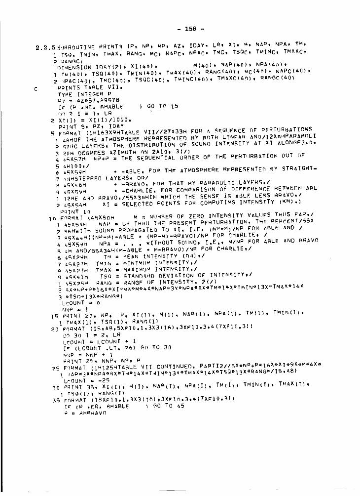
- 156 -

2.2.5Sd_OUTINE PRINT_ (Pt NP, MP_ AZ, IOAY, LRt XIt Mq NAP, NPA_ TM,

t TSQ, THIN, TMAX, RANG, MC_ NAPC, NPAC, TMC, TSQC, TMINC, TMAXC,

? PAN_C)

I)IMENSION IDAY(2), XI(40), M(_O)_ NAP(AQ), NPA(_o)9

I TM(40)t TSQ(40), TMIN(_O)_ TMAX(40)_ QANG(40)t MC(_), NAPC(40),

_IPAC(_O), TMC(40), TSQC(40)_ TMTNC(_n), TMAXC(40), _ANGc(40)

P_INTS TaQLE VII,

TYPE INTEGER P

P7 = AZ*57.29578

Ir (P ,NE. RHABLE ) O0 TO 15r)q ? I = 1.9 LR

2 XI(1) = XI(I)/tO00.PRINT 5, PZ, IDAY

5 Pq_MAT (IHI63XgHTARLE VII//_TX33H FOrt A SKQUFNCE OF PERTURBATIONS

I _HOF THE ATMOSPHER_ RE_RESENTED BY BOTH LINEAR ANO/12X_HPAPABOLI

_?HC LAYERS9 THE QISTRIBUTION OF SOUNO INTENSITY AT X) ALONG_3,0,

3 _OH DE6REES AZIMUTH nN 2AlOt 3(/7

4 A_X57H NP÷R = THE SEQUENTIAL ORDER OF THE PERTqJRBATION OUT OF

5 _HIO0,/6 c_X59H ÷ -ABLE, FO_ TH_ ATMOSPHERE R_PRESENTE_ BY STRAIGHT-

? _gHSTEPPEO LAYERS_ 0_/

R _SX_BH + -BRAVO, FOR T_AT RY PARABOLIC LAYERS,/

Q _SX_gm ÷ -CMARI..IE, FOR COMPARISON OF DIFFERENCE BETWEEN ABL

] ]2HE Ai_O BRAVO,/55X3RHIN WHICH THE SENSE I_ ABLE LE_$ 8_aVO,/

? _SX54H XI =SELECTEO POINTS FOR COMPUTI_G INTFNSTTy (KM),)

PRINT i_I0 ffnmMaT (45XSOH M : NUMBER OF ZERO INTENSITY VALUFS THUS _AR,/

] _SXS_H NAP = UP THOU THE PRESENT P_wTUR_ATION, TH_ PEPCENT/55X

? _6MWITm SOUNn PROPAGATEO TO Xl, I.E. (NP-M)/NP FOR ABLE AND /_SXa_H((NP-M)-A_LE + (NP-M}-_RAVO)/NP FOR CHARLIE, /

A _5X59_ NPA = . . . WITHOUT SOUND_ I.E,, M/NP FOR ABLE aND _RAVO

_H ANO/55X3_H(M-ASLE • _-BPAV0)/NP FOR CHARLIE_/6 _X?gH TI4 = _EAN INTENSITY (_4)*/

7 _5X_7_ TM_N = MINIMI}M TNTENqITY,/R _SXP'(H T_AX = MAXIMUM INTENSITY,/

_=tH TSQ = STAN_RD OEVIATTON OP INTEN_ITY_/

] _SXP_H mANG : RANGF OF TNTE_SITY. 2(/)

_X*(qP÷P*I6X*XIe_X*M*_X*NAP*3X*N_A*BX*TM*I_X*TMIN*I3X*TMAX*I_X*TSQ*]3X*RANG*)

LCOUNT = 0NNP : i

15 PRINT 20_ NP_ P, XI(]), M(1), NAP(t), NPA(1), TM(1), THIN(1),

I T_X(I), TSQ(I), RANG(t)

_0 _hQ_AT (I_AB,SX_IO,1,3X3(I&),3XFIO.3,_(TXFIO,3))

On 30 I : 2, LR

LqOU_wT : LCOUNT + l

I= (LCOUNT .LT. _6) GQ TO 30

N:_P = NNP ÷ }PRINT 25, NNP, N ° , P

25 F;)RMAT (tHI25HTAHLE VII CONTINUED, PAQTI2//_X.NP+P*I_X*XI*9×*M*_X*

I. 4AP*3X*NPA*_X*TM*I4X*T,41N*}3_*TMAX*}4X*TSQ*I3X*RaNG*/IS,A8)LKOUNT : -25

30 PRINT 3_, XI(1), M(1). NA_(1), NPA(1)_ TM(1)_ THIN(T), TMAX(T)_

I T_0(I), _ANG(1)

R5 _qR_AT (IRXFIO.I,_X3(16)_3X_In,3,_(TXFIO._))

[c (P .EQ. _HABLE I GO TO ¢5P : _H_AVO

- 157 -

PRINT 20t NP, Pt XI(1). MC(1)_ NAoC(].)t N_AC(1)t TMC(1)_ TMINC(1)_

1 T_AXC(I), TSQC(])_ RANGC(1)Oq 40 I = 2, LRLCOUNT = LCOUNT ÷ 1IF (LCOUNT .LT. 26) G_ TO 40

NNP = NNP ÷ I

PRINT _5_ NNP, NPMt PLCOUNT = -2_

40 P_INT 35t XI(1)o _C(1). NAPC(T)I NPAC(1), TMC(I)I TMTNC(T)iI TMAXC(1)o TSQC(1)_ RANGC(1)

45 R_TURN

E'_ID

- 158 -

2.2.6 $iI_Rr)UTINE F(_CI SUM (_iP, Mp, _FOCUS, _AMF_ XF(_CUSt TTNFt NPlPT,

I ,JPANI, NPIRP, NPARP, NFICI, NFACI_ TMFIN, TMFAX, TFTMIN, TFI_4AX,

2 TFAMIN, TFA_IAX, TFISO, TFA._O_DT_E.NSION NXFAX(4__)9 NXFIN(42}_ NA,,IE(II)_ X_OCUS(11},

I TFAX(II), TFIN(II), TINF(II}, h.'_ACI(_2}, NFICI(42)_ NPAPI(4_)_

2 'JPI_I(42)t TFAXI(42), TFINI(42), TFISQ(_P), TFA_Q(4_), T_FI_i(_P_),

3 T_F/_A(42), NPARQ(42), NPIRP(_2), TFIMIN(_2)t TFI_.IAX(42),

4 TFAW. IN(_2), TFA_'IAX(4_)

C I_ (II) COUplES M_K- (._IN-) TYmE FOCI FOR EACH PE_TURRATION C_SE,

I,_ : 0

IT = 0

i_ (iFOCUS ,EQ, h) GO TO 6_2C NXFAX (NXFIN) INTEGERIZES OISTAh_CE TO _AX- (PIN-} TYPE FOCI,

f_O 6_0 I = I, IFnCUS

N_I = NA'AE(1)Im (_vAMI ,EO, 3H'_IN) GL) TO 63_

la : IA ÷ 1NXFAX(IA) : XFOCUS(I) , 1

TrAX(IA) = TINF(1)

(_o TO 640

_35 I! = II + INXFIN(II) : XFOCUS(1) + I

T_IN(II) -- TINF(1)6a.O C_NTINUE

C ,1 IS RANGE IN IK._ INTERVALS,6"2 Oh 675 N = i, 42

I_ (NP .NE. i) Gn TO _,4_

C N_ACI(N) (NFICI(N)) ACCUMULATES NUMBE_ OF MAX- (V.IN-) TYPE FQCI PER UNTT

C _ANGE FOR ALL PERTURBATIONS liP THRU _P,_rACI(N) : 0

N_'ICI (N) : 0

C N_ARI(N} (NPIRI(k')) ACCUMULATES NUMBER OF MAX- (MIN-) TY_F CASES OF PER-

C TURRATION PER EACH K_-UNIT O_ RANGE UP TNRU NP CASES,NOARI(N) - 0

N_IRI(N) - nC F_'AXI(N) (TFINI(N)) ACCUMULAT_'S VALUE OF MAX- (MIN-) TYPE FOCAL INTENSITY

C _ER EACH UNIT RANGE N FOR ALL PERTURBATIONS UP T_RU NP,

T_AXI(N) = 0TrTNI(N) = 0

C ETC,_ FOP STANOA_O DEVIATION,

T_ISQ(N) : O,

T_ASQ(N} = O,

C I_FIN(N) (TMFAX(N)) ACCUMULATES MEAN VALUE OF MIN- (_AX-) TYPE • • • • ETC

T._FIN(N) = O,

T_FAX(N} = O,

C NPARP(N)_ (NPIRP(N)) ACCUMULATES PERCENT OF NPARI(N) (NPIRI(N)) OUT OF

C M_ PPR EACH UNIT RANGE,NPARP(N) - 0

N_IRP(N) -- (IC T_AMIN(N) (TFAMAX(N)) ACCUMULATES MIN- (M_X-) VALUE OF MAX-TYPE FOCI PER

C 'UNIT RANGE,

T=AMIN(N) = I,EI_TF_M_X(N) : O,

C TFI_41N(N) (TFIMAX(N)) ACCUMULATES MIN- (M_X-) VALUE OF MIN-TYPE FOCI PFRC UNIT RANGE,

TrIMIN(N} = I,E10

TrIMAX(N} -- O,

- 159 _,

6_4 Ir (IA ,EQ, n) G4 TO 6551

645 1)0 655 I : I, IA

NXFAXI : NXFAX(1)

I: (I ,EQ. I) 60 TO 646

I_ = I - IN_FAXM : NXFAX(I_)

6_ I= (NXF_XI ,NE, N) GO TO 655

N;ACI(N) : NFACI(N) * 1

IF (TFAX(1) .EQ, 0,) GO TO 65nT;ASQ(N) = TFASQ(N) + TFAX(1)**R

USE LIBRARY FUNCTIONS FOR FINNING MIN. AND MAX-V_LUES OF MAX.TYPF FOCALINTENSITIES PER RANGe UNIT,

?FAMIN(N) : AMINI (TFAMIN(N)9 TFAX(1))

T_AMAX(N):AMAXI(TFAMAW(N)_ TFAX(1))

TFAXI(N) = TFAXI(N) + TFAX(1)

6_0 IF (I ,EQ. i) GO TO 654

I_ (NXFAXI ,EQ, NXFAXM) GO TO 65_

654 NQARI(N) : NPARI(N) * I

655 CONTINUE

6551 I_ (NP ,NF, _P) GO TO 6591IF (TFAMIN(N) ,EQ, 1,FIO) TFA_IN(N) : O.

IF (TFAHAX(N) ,GT. loeb) TFAM_X(N) = O,

IF (NFACI(N) ,EQ, O) GO TO 65_

T_FAX(N) : TFAXI(N)/NFACI(N)

S,}AX : TFASO(N)/_FACI(N) - TM_AX(N)**2

Gn TO 65g6_B T_FAX(N) = h,

S_AX = O,

6_g IF(SQAX *LT, n,) SQAX : O,

T_ASO(N) : SQRT (SQAX)

NPARR(N) : IO0_NPARI(N)/NP

65QI I; (If ,EQ, O) GO TO _75

6&O DO 670 I = 1* II

NXFINI : NXFIN(1)

IF (I *EQ, I) GO TO 661

I_ = I " INXFINM : NXFIN(I_)

661 I; (NXFINI ,NF, N) GO TO 670

N;ICI(N) : NFICI(N) ÷ IIr (TFIf_(1) *EQ, 0,) GO TO 66_

TcISQ(N)=TFISQ(N) ÷ TFIN(1)*_

USE L.I_RARy FUNCTIONS , , , OF MIN-TYPE FOCAL INTEN_ITIE_ RFR RANGE UNIT.T;IMIN(N) : AHINI(TFI_IN(N), TFIN(1))

T;IMAX(N) = AMAXI(TFI_AX(N), ?FIN(1))

r_INI(N) : TFINI(N) • TFIN(I)

665 IF (I ,EO, I) GO TO 66g

IF (NXFINI ,EQ, NXFIN_) GO TO 670

669 NPIRI(N) = NPIRI(N) ÷ I6?0 CONTINUE

Ir (NP ,NE, MP) GO TO 675

IF (TFIMIN(N) ,EQ, I,EI0) TFI_IN(N) : O,IF (TFIMAX(N) ,GT, 1,E4) TFIMAX(N) : O,

IF (NFICI(N) ,EQ, O) GO TO 673TMFIN(N) : TFINI(N)/NrlCI(N)

SQIN = TFISQ(N)/NFICI(N) . TMrIN(N)**2G_ TO 674

673 T_FIN(N) = O,SQIN = O,

_74 I_ (S_I(_ ,LT, 0,) SQI_ = n.

T_ISQ(N) = SQ_T (SQIN)

N_IRP(N) = IO0_NPIRI(N)/NP

675 CqNTINUE

R_TURN

E_9

- 160 -

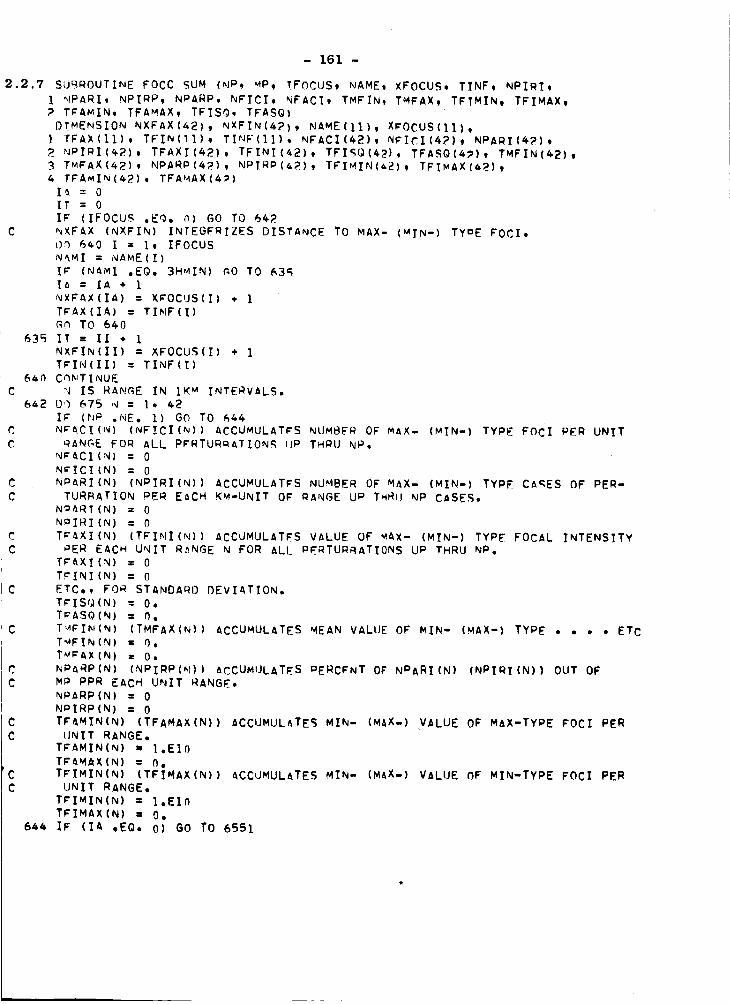
- 161 -

2.2.7 SUgROUTINE FOCC SUM (NP, MP, TFOCUS, NAME, XFOCUS, TTNF, NPIRI,

I NPARI, NPIRP, NPARP, NFICI, NFACI, TMFIN9 TMFAX_ TFTMIN, TFIMAXo? T_A_IN, TFAMAX, TFISq, TFASQ)

DIMENSION NXFAX(42), NXFIN(42}, NAME(II), X_OCUS(11),

] TFAX(II), TFIN(11), TINF(II), NFACI(42), _ICI(4?)t NPARI(4?),

NPTRI(_2), T_AXI(42), TFINT(42), TFISQ(_}, TFASQ(4_), TMFIN(42)t

3 TMFAX(42), NPARP(4?), NPTRP(42), TFIMIN(42), TFIMAX(4_)_4 TEAMIN(42), TEA_AX(4_)

I_ = 0IT = 0

I_ (IFOCUS .E_. n) GO TO 64?

C NXFAX (NXEIN) INTEGFRIZES DISTANCE TO MAX1 (MIN-) TyoE EOCI.t)n 640 I = I, IFOCUS

N_MI = NAME(I)

IF (NA_I ,EQ. 3HMIN) AO TO _3_la = IA ÷ 1

NXFAX(IA) = X_OCUS(1) ÷ I

T_AX(IA) = TINF(I)GQ TO 640

635 IT = IT ÷ I

NXFIN(II) = XFOCUS(1) ÷ i

T_IN(II} = TINF(T)

64n Cq_TINUE

C _ IS RANGE IN IKM INTERVALS.642 D _3 675 N = 1. 42

IC (NQ .NE. i) GO TO _4

C N_CI (N) (NFICI (N)) &CCUMULAT_S NUMBER OF MAX- (MIN-} TYPE FOCI PER UNITC nAN_E FOR ALL P¢RTURQATION_ UP THRtJ NP.

N_aCI(_) = 0

N_ICTIN) : 0

C NPARI(N) (NPIRI(N)) ACCUMULATES NUMBER OF MAX- (MIN-) TYPE Ca_ES OF PER-

C TURBATION PER EACH K_-UNIT Of _ANGE UP THR_I NP CaSE_.N_ART(N) = 0

N_IRI(N) : 0

C T_XI(N) (TFINI(N)) ACCUMULATES VALUE OF MAX- (MIN-) TYPE FOCal INTENSITY

C _ER EACH UNIT R_NGE N FOR ALl_ PERTURgATIONS UP THRU NP.T_AXI(N) = 0

T_INI(N} : 0

C ETC., FOR STANDARO DEVIATION,

T_ISQ(N) = O.

T_ASQ(N} : O,

C TqEIN(N) (TMFAX(N)) aCCUMULATES MEAN VALUE OF MIN- (_AX-) TYPE • • • • ETCT_FIN(N) = q.T_AX(N) : O,

C NPARP(N) (NPIRP(_I)) ACCUMULATES PERCENT OF NPARI(N) (NPI_T(N)) OUT OF

C MP RPR EACH UNIT RANGE.

NPaRP(N) : 0

N_IRP(N) = 0

C TFAMIN(N) (TFAMAX(N)) aCCUMULATES MIN- (MAX-).VALUE OF MaX-TYPE FOCI PERC UNIT RANGE.

T_AMIN(N) = I.EIO

TF&MAX(N) : _,C T_IMIN(N) (TFIMAX(N)) ACCUMULATES MIN- (MAX-) VALUE OF MIN-TYPE FOCI PERC UNIT RANGE,

TmIMIN(N) = 1,E10TFIMAX(N) = O,

644 IF (IA ,EQ, O) GO TO 6551

- 162 -

645 On 655 I = I, IA

NXFaXI = NXFAX(1)

I_ (I ,EO. I} GO TO 6_6

I_ = I - 1NXFAXM = NXPAX(IM)

_A6 IV (NXFAXI ,NE, N) GO TO 655NVACI(N) ffiNF_CI(N) + i

IF (TFAX(1) ,EQ, 0,) GO TO _Sn

TFASQ(N) = TFASQ(N) + TFAX(I)*_2C U_E LIBRARY FUNCTIONS FOR FINNING _IN. AND MAX-VALUE_ OF MAX.TYPE FOCALC TNTFNSITIES PER RANGF UNIT,

TrAMIN(N) = AMINI(TFAMIN(N), TFAX(1))

TFAHAX ..... _'^_,_I-A.-._X_(TFAHAX '_'I,.I,TFAX(_')1;T_AXI(N) = TFAXI(N) * TFAX(1)

650 IV (I ,EQ, I} GO TO 6_4

I_ (NXFAXI ,EQ, NXFAXM) GO TO 655

@$4 NPARI(N) = NPARI(N) ÷ I

655 CnNTINUE6SS_ IF (NP .NF, M_) GO TO _59_

IF (TFAHIN(N) ,EQ, l,FlO) TFAMIN(N) = _,

IF (TFAMAX(N) ,GT, I,E4) TFAMAX(N) = _,

IF (NFACI(N) ,EQ, O) _0 TO 65_

T_FAX(N) = TFAXI(N)/NFACI(N}

S._AX = TFASQ(N)/NFACI(N) - TM_AX(N)_?Gn TO 659

6_ TMFAX(N) = _,

Sm_X = O,

6_g Ir(SOAX ,LT. 0,) SQAX = O,r_AS_(N) = S_RT (SQAX)

N_ARP(N) = }O0_NPARI(M)/NP

65QI I_ (If ,EQ, O} G_ TO &75

6_0 nn 670 I = I, II

N(FINI = NXFIN(1)

I_ (I ,EQ, I) GO TO 6_I

I_ = I - iNXFIN_ = NXFIN(I_)

6_I I_ (NXFINI ,NF, N) GO TO 670NFICI(N) : NFICI(N) ÷ 1IF (TFIN(1) ,EQ- 0,) GO TO 66m

TrISQ(NI=TFISQ(N) + T_IN(1)**?

C U_E LIBRARY FUNCTIONS , , , O_ MIN-TYPE FOCAL INTENSTTIES PEP QANGE UNIT.TFININ(N) = AMINI (TFIMIN(N), TFIN(1))

TFIMAX(N) = AMAX](TFIMAX(N}, TFIN(1))

T_INI(N) = TFINI(N) ÷ TFIN(1)

665 IF (I ,_0. 1) GO TO 6A9IC (NXFINI ,EQ, NXFINM) GO TO _7_

669 NPIRI(N) = NPIRI(N) + 1670 CqNTINUE

IC (NP ,NF, HP) AO TO 675Ir (TFIMIN(N) .EO, I,_I0) TFI_IN(N) = O,

I_ (TFIMAX(N) ,GT, i,E4) TFTM^X(N) = n,IF (NFICI(N) ,EQ, O) _0 TO _?_

T_PIN(N) = TFINI(N)/NF.ICI(N)

S_IN = IFISQ(N)/NFICI(N) - TM_IN(N}_?Gn TO 67_

673 T'_FIN(N) = O,

SQIN = O,67_ IF (SQZN ,LT, 0,) SQIN = O.

T_ISQ(N) = SQRT(SQIN)NP_RP(N)= IO0_NPIRI(N)/Np

675 CONTINUER_TURNE_O

- 163 -

- 164 -

2.2.8 S!J_ROUTINE P_INT_ (P.TT. Q, R. AZ. ID_Y_ MP. NPIQI, NPIRPt N;ICI.

1T_FIN, TFIMIN, TFIMAW. TFISQ)

DIMENSION IDAY(2), NPIRI(4P)t NPIRP(42), NFTCI(42), TMFIN(42).

1 TwIMIN(42). TFIMAX(_), TFISQ(42)TYPE IN[EGER P, Q, R

P! = AZ_57°29B78llq9 PPINT 170_ P.IT. MP. Q9 R. PT, I_AY,IT9 MPt MP_TTgIT, IT. IT1700 FORMAT (1H160X12MTABLES VIII-&6//57X_2HA _I_T_IBUTION SUM_ARY/_6X

11HF()R/5OXA4. 32HTYPE wOCI OF SOUND PROPAGATED IN/45XI4t_H SUCCESS35HIVE PERTURBATIONS OF THE ATMOSPHERE/AQX14HREP_ESENTED BY ARo

3 _R, 7H LAYERS 3(/)

4 A3XIOHAZIMUTH = F4.0. 9H DEGQEE_. 4X]3H DATE-TIME = 2A1n, IH_/45X_gH R = RANGE IN IKM INTERVALS, E.G.. 1 = 0 TO I, ? = i TO

6 _M2. ETC.,/T 4SXISHCASES = NUMBER OF A3, 32H TYPE FOCI-CASES OF OERTUQBATION /

B RAX26HPER EACH UNIT _ANGE OUT OF 14, 15H-P_RTUR_ATIONS'/

g 4SX22HPERCT = PERCENT 0F THE I_, 28H-PERTU_BATIONS THAT _AVE ONE/

I _XgH OR MORE A3,44H-TYPE FOCI IN THE UNit R_NGE SPECIFIED AY R,/2 45XlSH FOCI = NUMBER OF A3, _4H-TYPE FOCI PER SPECIFIED _ANGE UNI

3 _HT,/45X36HMEANI = M_AN I_TEN$1TY IN OB OF ALL A3. 16H-TYPE _OCl OCCUR

5 _HRING IN THE IKM-RANGE SPECIFIED,/

_SX3OHLEAST = LEAST INTENSITY OF ALl_ A4, 2_H-TY_E FOCl _CCURRING

7 _3HIN SPFCIFIED IK_ RANGE,)

_INT 1201, IT12_I FORMAT (IH 44X4#H_OSTI = LArGeST VALUE OF INTENSITY OF . • ,/

g _SXagHSIGMA = STANDARD OEVIATION IN INIENSITIES OF ALL A_,5W-TYPE

] _H FOCI/54X_3H EALLI_G WITHI_ THE SQECIFIEO IKM INTERVAL.2(/}

_(IOX_CA-_2X_PE-_46X)/2(TX_R_2X_SES_?X_RCT_?x_FOCI_X_ANI_SX

3 _LEAST_SX_MOSTI_SX_SIGMA_IX))

1202 M_ = 21

_h 1220 N = I. 21

L = N + MMPRINT 122_, N, NPIHI(N), NPIR_(N), NFICI(N)* TMFIN(N}, TWIMIN(N),

T_I_AX(N), TFISQ(N), L, NPlPT(1), NPI_P(L). NFICI(L}, T_IN(L),

? T_IMIN(L), T_IMAX(L). TFTSO(L)

12_0 CqNTI_UE

12P5 FOP_AI (2(3XIS.15,15.15,1XFIO.3.F10.3.FIO.3.FIO.3))

1230 R_TU_

- 165 -

2.2.5 IDENT

PROGP_M LENGTH

BLOCK_

PROGR_Mo LOCAL

// COMMON

ENTRY POINTS

00_001 INSYM

ENTRY

USEIOAY RSS

Y RSS

T RSSWDIR _SSWSPD _SSLMAX BSS

AZ BSSOPHIMTN @SSKMIN RSS

KMAX _SSKMINC _SSKMAXC RSSMP _SS

Xl BSSLR RSSSIGMA BSSNC _SSALT _SSCORPl RSSCOR_ RSSCOR_3 RSS

USEDATA

INSyM RATAVFD

VFDVFDVFD

VFDVFD

VFOVFOVFDVFDVFDVFDVFnVFOVFDVFD

VFDVFDVFD

TN_YM

INSYM

//?

_7

37

i

II

I

I]

I

I_0

I

I

2500

_500

_500#

0

4?/4HTDAY,I_/IDAY

42/IHY,IB/Y

4P/IHT,18/T

AP/4HWSPO_lB/WSPD_/#HL_AXolS/LMAX

4_/2HAZolQ/AZ_/7Hn_HIMINt]R/DPWIMIN

&?/4HKMIN,IR/KMIN42/_HKMAXoIB/KMAX

42/5HKMINC_IB/KMINC

A_/SHK_AXC_IR/KMAXC

_/2HL_IR/LRa_/SHSIGM_lS/SIGMA

_/_HNC}_/NC#_/3HALT_]8/AI.T_2/SHCORR_]B/CORR]

05126/68 PAGE NO,

VFDVFD_ND

UNUS_O STORAGE

- 166 -

_215HCORR?,IQ/COR_2

_215HCORR_,IB/CORR_

4Q STATEMENTS 2_ SYMBOLS

PAGE NO,

2.2.6

IDAY

Y

WhIR

WSPn

LMAX

AZOPHI_TN

KMIN

KMAX

KMINC

KMAX_MP

Xl

LR

SIGMANC

ALT

CORRI

- 167 -

SYM_ULIC INPUT

?FEB 27,1964t 16_5C_T

h,,_O6,,230,,3_,,_B_,,616.,776._Rg_,_]_31.,IIS_,,I_65,913_A.

1514,,I_61.,17S9,,1920,,_06_,,219_,,23]0,,2458,,2597,,27_8.

?87P,,3h_h,,315_,,3P96,,3440,,350_.,37_7,,3RT_,,30flq,,&14_.

pTfl.75,976.65,?75.15,_75.05,275.15,975,75,278,0_,_7_,B%,_7_.55

?76olS,_75,35,?T_o_,273oT_,?lP,45,97],65t_TO,55_69,4_,26R,55

_67.25e966,05,765,0_9_64075,_6_,5_,_64,55_263,45_6_,0_,_6],95

960.6_,960._59_59,35,259,75._5803_,_58,35,2_7,0S,_5_,75,_55,75

50oOS,83._O,90,(}O,IOT,50,_33,50,I_7oTO,178,10_IRg,30,_Q_,g_

IWS.60,198,50,?O_.OO,_O_,gO,_Oq,?O,21_,_O_??_,80,_3],_O,231,40

9q7,TO,)ag.50,262.10,273,20,_77,80,_7_,70,_77,00_?7_,60,_6_,|O_63,20,?65,70,_6_,afl,?60,qfi,_8,30,_55,5(),_l,70,9_,O0,_7,TO

_,]0,I.I0,_.I(},5.30,7,_0,9,a0,II,70,II,90,10,60,9,70_9,_0,0,10

R._,7,qO,7,20.7.00,6.BO,6.00,5,80,_,30,7,#O,II,30,15,_O,18,70

36

45,n. O04

I020

I0

I00

1,0÷3,2._÷3,3,0*3,A.0÷3,5,0÷3,6,0÷3.7.0÷3,8.0÷3,9,0÷3,10,0,3

11.0÷_,]2,0÷3,13,0÷3,1_,0+3,15,0+3,16,0+3,17,0÷3,1_,0÷3,1Q,0÷3

PO,O+3,21,O+3,_?,O+3,_3,0+3,_,_+3,P5,0+3,_6.0+3,?7.0+9,_8,0÷3

79,0+3,_0,0+3,31,0÷_,3_,0+_,33,0+3,_,0+3_35.0+_,_6.0÷_,37.0÷3

3R,0+3,_9,0+3,_0,0+3

_0

_0(0.3),I00(0.6)a2

l,O0,O._2,0,57,n,_,O,OS_AS(O,O)

O,8_,l,n_,O,B_,h,57,0o24,0,08,4_(O._)

O,57,0._,I,O0,_.82,0,S7_O,_,S,OS,_3(O,O)

O,24,0,_7,0,82,1.O0,O,B2_O,_T_O,2_,,OA,_2(O,O)

O,O,O,08,0,2_,O,57,0,82,1,O0,Q,8_,O.57,_,_4,0°OB_O(Q,O)

_(So0),0,08,0,_4,0,57,_,8_,],00,0,8_,0,57,0.24,0,08,39(0o0)

3(O.O),_,OB00,_,O,57,h,8_,],OO,O,B_,O,57,0,24,0oOA,38(O,h)

a(O.D)_n,OS,0,_a,Oo57,_,8_1,00,O,8_00,57,0,_,O,08,_7(O,O)

_(O,O),a,OB,O,_4_O,57,0,8_,],OO,O.B_,O.SY,O,_,O,08,36(O,O)

&(O,O),O,0_,O,_4,0o57,_,8?,],OO_S,8_,O,57_Oo_4,0oO8,35(OoO)7((),O},_,SS,0.2_,O,57,D,82,1oOO,OoR_,O,57,0._,O,O8,3_(O,O)

A(O,O),_,O_,O,_a,O,57,0,8_,I,O0,O,89_O,57_O,2_,O,O8,33(O.O)

_(O,O)_n,OS_0,_,O,57,0,8_,l,OO,O,8_O,5T,O,24,0,O8,_(O,O)I0(0,0),0,08_0,_4,0.57,0,8_,I,00,0o_,0,57,0,2_0,08_3_ 0,_)

_I(0,0),0,08,0.2_,0,5?,0,82,1,00,0,_2,0,57,0,24,0,0A,30 0,0)

_(OoO),floOB,O,_90,57,0oB_,_eOO,O,_2,0,57_O,2_,O,OS_q O,fl)

13(0,0),0,08_0.24,0.57,0,8_,I,00,0,R_,0,57,0,2_,0.08,_8 O.O)14(O,O),O,08,0._,O,57,0,82,1,O0,O,"2,S,57_O,2A,O,OR,_7 0,_)

15(O,O),Oo08,0,R_,O.SX,O,8_,I,SO,O,_2,h.57,_,_,O,OB,_6 O,S)

16(0o0),0o08,0°_,0,57,0,_2,1,00,_,_2,_,57,0,24_0.0B,_ 0,_)|7(0,0),0,08_0,24_0,57,0,8_,i,00,_,_,0.57,0,_4,0,08,?& 0,_)

18(O,0),O,OB,O._,O.57,D,A2,1,O,,_.R2,0.57,0.2a,O.OR,_3 0._)

- 168 -

COR_

IO(0,0

_0(0.0

_I (n.0

22(0.0

73(0,0

_4. (0,,0

_5(0.0

_6(0.0

_7(0.0

?_(0.0

_9(0,,0

,O,O8,O,24,0.57,0.82°l,O0,O._2,0.57tO.24,0.Oa_22(O°o}

,N.08,0.24,0.57,0.87,I.0090._2,0.57_0.24,0.0_21(0,0)

,O.NS_O._4,0._7,0,_,l. OO_O.q2,O,ST,O.24,0.Oflt_O(Oto)

,O,NStO.24,0.57,0.82.1.OO,o._2,O.57,O.24,0,OAtlq(O.o)

,0.08t0.24,0.57.0.82,1.00,0._2,0.57,0.24,0.0_,I_(0,0)

,O,O8.O.?4,0.57,O.82,1.O0,O.Q2,0.B?,O,24,0,OA,17(O.o)

.0,08,0.2_0.57,0._2,1.00,0._2,0,_?,0.24,0,0A,16(0,0)

,O°O8,O.24_O.57,O.82,1.00.O._2,0.57,O.2A,O.OA_IB(O,O)

,O,O8,O._4,O,57,0.B_,I.OO,O._2,0.57,0.24,0.OBtI4(O.o)

,O.OH,O,24,0,57,0.B2,1.OOtO.R2,0.57,0,24,0.O_I3(O.O)

_o(o.o},o.n8,o,_,O,ST,0°_?,l,00,0,A2,o,57,o,2_,0,o_11(o,o)

31(o,0),o.o8,o,24,o.57,0.82,1.00,o,_2,o,57,o,24,0,08_I0(0,o)

32(o.o),o.o8,o.24,o.57.o,82.1.oo,o,_2,o,57,_.24,0.oB,9(o,o}

33(0,0),o,08,0,_4,0,57,0°B2,1.o0_0°_2,0,ST,O,24,0.0B_B(n.0}

35(o,o),o,o8,o°2_,0.57,o°_2,1,00,o.m2,0,57,0°24,0,0_(0,0)

36(0,0},o°oH,o._4,0,57,0°8_.I,00,0,_2,o°57,o,2_,0°0_5(0,0}

37(O.0),0.08,0.24,0.57,0,82,1,00_0.A_,0,57_0,24,0°0A_4(0,0)

3_(0,0),0.0_0.24,0.57,0,82,1.00,0.R2,0,57,0,24,0,08_3(0.0}

3_(0.0},0.08_0.2A,0.57,0,8_,1.00,0.R_,0.57,0.2A,0.0m,_(0,0}

41(0.0).0,O8_0,2_,0.57,0,8_,l,00,0,R2,0,57,0,24,0,0m

43(0,0),0,08_0,24_0.57,0,8P,I.00_0,_2_0,57

4_(0.0),0.0_,0.24,0.57,0.82,1.00,0._2

_5(0,0),0.0_,0,2_,0,57,0.82,1,00

],00,0._2,0,57,0.24,0.08,45(0.0)

0.57,0,_2,1.00,0,_2,0._7_0._4,0,0B,43(0.0}

0,08,0,_,0.57,0,B2,1.00,0._2,0,57,n,24,0,0_,_1(0,0)

0.0,0.0_,0._0°57_0,B_,I.00,0,_2,0.BT,0.2_,(),0B_40(0,0)

_(0,0),0,0H_0,24,0.57,0°82,1°00_0°8_0,57,0,2_0,08,3@(0°0)

_(0,0},O,0A_0,24,0.57,0.B2,1.00,0,B_0,57_0,24,0,0A,37(0°0)

6(0,0},h,08_0,_A_0.57,O,82,1,00_0,8_0,57_0,24_0,08,35(0,0)

7(0.0),n,0_,0,_4,0.57,o,82,],00,0,_,0.57,_.2_,_.08,34(0,0)

_(0.0),n°0_,0°2_,0,57,0,82,],00,0,8_o,57_0,2_,0,08,33(0,0)

10 0.0) n.0@,0.2_,0.57,0.82,1,00,0.A2,0,57,0,24,0,0B,3](0,0)

11 0.0) 0.08,0.24,0.57,0°82,1.00,0._2,0.57,0.2_,0.0_,30(0.0)

12 0.0 ,O.OS,0,2_,O.57,0.B2,].OO,O._,O.57,0.24,0.OA_(O.n)

13 0.0 ,O.08,0._W,O.57,O.8_I.OO,O.m2,o.BT,o.24,0.OB,_A(O.O)

]5 0.0 ,h,OB,O._4,0.57,0._p,l.OO,O.m_,O.57,O.24,0.O_6(O.0)

]_ O,O ,O.08,0.24,0,57,0.8_.I.O0,O._2,0,57,O.24,0.OR_B(O.O)

]7 0,0 ,O.O_,O._4,0,57,0.82,1.O0_O.m2,0,57,0,24,0.OB_P4(O,O)

_B 0.0 ,O.O_,O._4,0.57,0.Sp,I.OO,O._2,0,57,0.24,0.OR,P3(O._)

_I(o.0 ,O.O8,O.p4,0.BT,0.SP,I.OO,_.R2,O._7,O,24,0.O_,_O(O_O)

_3(0,0 ,O.OB,O._4,0,BT,O.8_,I.OO,O.R2,0.BT,O_4,0,OB_IB(O.O)

_B(O.O ,O.08,0._,O._7,O_B_,I.OO,O._,O.BT,O.24,0.OB,IA(O.O)

_6(000 ,O._8.0._4,0.BT,0eA_,I.00,OoR_.O.BT,0._4,0.OA_B(O.O)

_7(0.0 oOoOS,0._,O,57,O.82,1,O0,O._2,o.57_O.24,O,O_,Ia(O.n)

_(0,0 ,0,08,0.24,N._7,0._,],00,0._,0°57,0_24,0.0_,I_(0,0)

_9(0.0 ,O.O8,O.2_,O.57.0.8_.I.O0,O._2,0.57,O.2A,O.OB,I_(O.o)

BO(O.O ,O_O_,O.24,O,57,O,B_.I.OO,O.A2,0.BT,0,24,0.OB_II(O.o)

31(O.O),O.08,0._4,0.57,0.8_,l.O0,O._2,n.57,0.2_,O.OB,lO(O.O)

32(0,0}.0,06,0._,0.57,0.8_.I,00,0._2,0.57,0,2_,0.08_g(0.0)

33(0_0).0.08,0._4,0.57,0.8_,I.00,0.e_,0,57,0.2_,0.0_8(0.0)

34(0.0),0.0B,0._4,0.57,0.8_,I.00,0._2,0.57.0.24,0.0_,7(0._

- 169 -

EN_

35(n,o)

q6(n,r))37(n,,_)

39(0°0)-_a(n,q}

4l (n.N)/,._ ( I! ,. o,)

_4(0°0)

_,_(n°n)

°N°O'd,9.P#,0.57,

, Oot_Xtllo_4,_No_7,

°.3.089 _.2_,,0°57q

, (#.OH,O.2_., n .67,

,.O.NBgO._4,O,b7,

,0.N_,!_._4,0,57,

, n.O_, f,.P_, f).57,

O._P.I.00

O.H_.1.000.82.}.00

0.8_.I.00

0°H2.1o00

N._P.I.ON

n.R2.1.O0

,O'_2.0.57,[email protected],e(u.o)

,h.m2,0.57,[email protected]_,5(O.h)

,O.Q2.0.57,0.24,O.hB,3(O.O)

,O.qp.n.57,h°24.0.OR,P(O.O)

,O.q2.h.5?_O.24_O.OB.N.O

,_.m2,_.67

O.SZ.I.O0

CHAPTER III

NUMER I CAL RESULTS

- 171-

3.0 NUMERICAL RESULTS

In a sense, this chapter is somewhat of an

appendix to the report. The tabular data generated

by the program presented in the previous chapter

and used by the case study discussed in the first

chapter is compiled here.

The four main tables in this chapter have

been written so as to make their content easily

understood. It might be of interest to mention

where the contents of these tables appear in the

discussion of Chapter I. Material from Table V

appears in Figs. 1-5, 7-10, and 13-16. Some results

from Table VI are used in connection with Fig. 30.

Actually, a lot of useful information in Table VI was

never treated in Chapter I, so that the reader may well

wish to peruse through this table. From Table VII, a

lot of information went into the making of Figs. 17-26.

And, Table VIII was the primary source for the results

presented in Figs. 27-30.

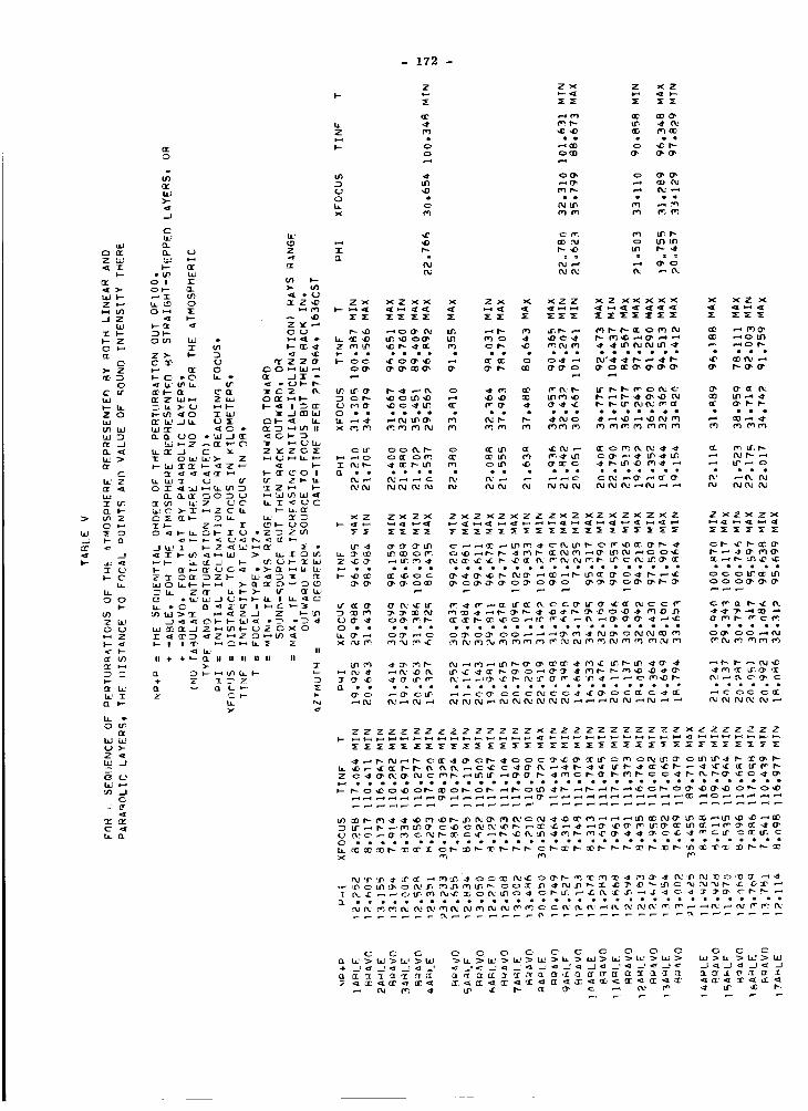
n-O

>-

..J

EL "..Dc= (J Z

o ! 1- (/3 I--

C._ U e_ Z ZO"

_I. OL UO _t_lJ_JE _r,G I-- :3

I 0_=' _ Z =-* _ Hi, m.,

_- __;_'_"'_,,.,,...,T" I,- (/') H :>

e --L_J _ _r J Z I-_ _ I-- U 2 C_ X 0

II + .ll. _ 0_ II II II II II II>,- ::Z-

>¢ ._,

- 172 -

Z

(_

Z er_

U _0 •

x

7 ,o.

a &

ZX: Z _{_"

aD U_ _tlrl

I_-qD ,--_ 00' (M U3

Z mU_ MD I_- _'t O_t-- • • • • • • •

O,o0_ 0',(:I, 000 _

× mm m _ _ (I,1 m

ZX X XZZ XZ XXXXX

•,,Itt_3 _ t'r _.; I." E I" I" _'_ C' (_IJc

I I I ! ! ! ! I ! ! ! I !

}.c xZ x

aO ,.-* _ Ot_OC; ,-I¢D t£)

0" I_ 0" 0 "

O0 Llr) ,--_ d"

IM (M Od {'_J

"JO 3_ :3_ (:ID

g ,:;..: J_; _g

=E

....... ...............

gO ..t .--_I',*-_ _'--d" .ID -t r-- _' ".IDo ,o .O .irl

Z X_xzx

r" Q I_'- _IE {%

o_, o%_

_g. oc o=

ZZ ZZZ ZZ ZZZ Z_ Z Z ZxZZ Z ZZZZZZ _-- Z XZ ZZZ _Z Z

O_ (_j O. O_ C i'_,i_ .-.ilj3 ff .-= O" I_ ,_1 _ C I'_ O" t.,3I..-C C -.t i_ (% I'-O" _ O -.t

.... ..........

_2 _ _ _ _,_' r_,_ _, _" "_ ....................

- 173 -

Z ZZ

g mmZ M _

O • • •

NO

Z Z )< Z

O' O" ,-4 oO

• • e •

0,3 o'1 f_ 0,_

f_ 0_1 I_ (%:

Z Z

_ un

I'- Iw'-O" _'--',IDI_- C t'--"4: IJ_ LIt},--__OC (_'01_ "3_ I_- (I" O, 3_ O_ o[3 (:_ ,.-_

Zx_x Z XZ x ZX_ XX

g :,-- ,_t_ ",(:: CC gT, C") OJ C_, L_ '_"_ ._C _".

;- .......... _..

• • • • • • • • • • • •

• • • • • • • • • • • • •

0 r"- 0" I_- 0 ' _: ,.'-_ 0c O_ 0, c' ,,,£: 0"

,'-i 4 I"- 0" I..£. [Jr_ f...----IPCUn ",'t0";,C _" O_J _'3 r-_ f'*'_*C]r"

X _Z Z XZ X _X _ XZ

'_IO r,,- u_f_r (% .--_ ",,C I'_ O" COD I".-- (_ (_. _"

C_,_r_F -F- ¢C_ c_

{/') _ _"',,,-_il" LI_ (%1 _

_ t'- f"-- :I:) r"--,'I:) _ ,:or W'- ::I] iN`

• • • • • • •

. ...-._ ,.-_ i..... _,. _*,_

c

_. _ _ c,., _,. _ _ o ,.,_ ,,,_

- 174 -

z z z z z xZ

I--

t-_ • • • • • u •

0 a • • • _ • • •

b.Z

(._0

- 176 -

X Z _ X xX X

Z C"_ f-- -,t" ,,t ",,T _._ C _1.

O_ _ OE O_ _" a_

(DO" ",1£,.-4 _ _ I"- _ C0 • • • I • • • •

_m g

¢'1 • • • . • • • •

Zx ZX Z ZZ XZ ZZ

Z _It _- _. _ t_ -_I-_I" _, _ _. _"

0 • • • • • • • • • • •

_ _._. _.-'."2._. _._._ _.

I,--

Z

5_ tL

x

I..-

Z 0 0 0 0 0 0

G' O" O" O" 0

.J_D

LD

tJn

- 177 -

Z_E

...3'CU

rl

I--

t_J

I1_O

D J_J

-.2

[iJ O

_rt_ Zu. I£h _

_-4 _J

(.)

_ CIM 1._T _/

m

- 178-

r-

"F

U

Q

Z _ _ _ _

t_

Y

Z

g _

n_tlA

_ c

2

_ _ o 0r_ _ f_ _ ¢_-!

C OJ_ _ C _

_DZ

C

h k_

fflc ,-.._ I'_1 _ ,_ L_, ,,IP r-- _: _ I'_ _ t_ _ _ f,_ (,,rl (_n _i" _ _i" "_'

_5(X U _

>-

fFl t'_ (k I_-14-!f'- qD

2 -2,-4

J

U0U-

h. -JO_ Ur o'_(._ • • eZ ,,6 ,4)I.L_X

- 179-

_" 4B r,_ _X" ,f (k'

(k; C _ID 4" -,I'

4D

I%- 4D 4_ (%.1 4B<7" ,'%J ,,11" {W

#'% 0 _ _0 ,'-. 4t

,.ID (X3 (_. o

(2')_E

Z

_f • • •

0 _1

Ix'Q_

,4" o0

¢_ • • •Z _

h f%l I'_ I'_

,-.-t

4" _ f'- 4" _k'o _ _ o2

['% _) _ ('_ ."3 _ _D (_"

e[ t'_ G[ (k_ 8[ "4" •4t fkJ P" ,,It ('W

('W ",t" (',% t£

(.9

Z

>-

Z -JH

J

(.)0

b_

ao

I_ .,.1 9'r.

_ g

180 -

I_- UD _ _D_ "-_ _ OD ,-_ f_4 aD

• _ - _-- .; i ....

I_1 ,_( ,'-_ ,-'_ _ _1_ I_- _- I._ _

..... _ _ : • . .

aD

%C

_D

un

_0

Lr

(C

(n

Z

o _b,. _.Q

I.=_o J

b,J

ZbE'

...1 _

• • • • • • . • e • • ,

f_ _ I_ o_ (k' 0_ I_. _ I_- _ (x_

(Z _C _ _:_ _,1_ O' 0 _ ".,_ _ ,'-4 _"" L_.

,43-e

_P

CU

Z

0

bE-J

I--

l,i.l

tL

•e'_ _ I_ r_ _ b- _ _ _ _D az _ _u

o" (3" O" O" 0 _

nr

Z

NZ

Z

..3

U0h

U-0

Z

ItL

0

u_

0

u

u.

0

M

.J

J

Z

_q

£9

..J

I,-.-

J

Z

0.

#

W

o

,t-

0",

f_

cc_

Z

- 181 -

I--I[L)WDP1_D

,¢O_

_JOf:_ml.l.l [UZ_

...IZC

II-- 1-Ol 1

>- D-,_N

<fC.tdI--WZ l,,,.In.

hr,.,O_ QQ.h, In

l._(Dn,. ZWOT If

> 0 __ X

J '_ I---rip <

I-- I >-I-- I--

0 Z

ZZOM

¢ri_

0_"_I--

UJ_<J enZMbJ_

Qm

IOC_--C_u o

_X

>-

J

U

JC

- 182 -

_9°._.°.°.=.:_._=-:-_%_.. . _-:.9°._.°_._. .. .. . •

0

>-

O. Z {D

o_ _ emo I -/ _ 0

i. _ 0 r_0 _-_ Z I,

O. P- U c_ J tO:) I- *--%I

I-- bJ OD _r-:D _ (:_ n, eO I--

i. i_ Q" C :E I-- _t I '_ ,-'O'r _ _ _I_ 0 _-_ ,., r_, _ ,..., O.

O. rl ,.-, ,..., _ _ rl W _E Z h

C_: OleO. U') 01-- Z (9 Z ZO aD _ _Z >-

QI:I-- :E Z I. Z LIC <r _ :D > 0 >- )-- 0 I -

<[ I I-- O_ bJ Z O_ (10. IsJ I-- I I-- Z Z _-_ L_

I-- 0[" b- I-- 0 I_ IsJ _:5 (r 0 (/_, I-- I-- _ _7KO _ IZ41 + ZZZC_

gel L_J> _

]E ._ OD 0I-- I I I

II ÷ +

eL

(12

"- ....... _; - .:'- d_ ,A_'.;,;,_ ,,;,.:,-"J ;,_;

II II II II II II II II II

X _1 Q I- I-_ (I (/1Z17 Z _:_ I-- _ n Lr_ ID (_ ID I_- I_ O" e_ C c" _" c_ C _ _C O" IF I"- I_- P- _ _ _ _ _ _

I--I-- __ Z _ _ OC I-- -,1 P- IZ OD aE Ol: _ (Z: oO OO aD OE

:E U_ LI_ tr, u-_ I,--P-- o_ l_')c c c, c c f_ _ID (_P.tl_ I'- I"- I"- I'.-I"- I'_ _ _ _('_JWD (I) I',- ,,'I_Iw- (E' (Z__ _0 (X; _ (I) CC _ (E_

O b_+ .J

- 183"_

• • • o • • • • • • • • • • • so • • • • • • • • • • • • • • • • • • • • • • • • • • e • • o • • o • •

O_ ,..-_,,.-_ ,-., ,,.-e 9,,.-4 _ _-_ I I I l I I .-_,,"_,-_,'-0,'-_,"4,,"_ I Od(5_(_It'_(_r_{1_(IJ t%.ll l l l l l I l l l l l

0(/)I"-

I-.- • • • • • • • • • • • • • • • • • • • • • • • • • • • • • • e • • • • • • • • • o • • • • e • • • • • •

_.- • • • • • • e • • • • • • • • • • • • • • • • • • • • • • • el • • • • • • • e e • • • • • • • • • • •

• • • • • i • • • • • • • • • • • • • • • • • • • • • • • • • • • • • • • • • • • • • • • • • • • • • •

.-,t r.4 ,.._ ..,4

l--n_

_J

Z

7_0U

..3_D

I--

(3. G[:',:: Y.3

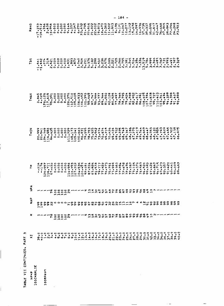
- 184 -

• • • • • • • • • • • • • • • • • • • • • • • • • o • • • •

I I

of]

I-.-

e = • • • • • • • • • • • • • • • • • • • • • • • • • • • • • • • • •

Z

OE

o

I._.,_Z

I-.-

J_B

hJ

_.1 (2

_L 1-Z (,..) n-

O 00 0

bJO_IL'

0.

ZCUl

I--UJ

bJI-- h: __J":IT

>- (gB--r _

ILl "_ _L I_ _LJ _r OOtl

QO I:E Z _,-0 I--

.J _ C I- I,'-

I-- _ UO. II

_ ob. __' C?>bJ

o0

b-i-,iL)hiD-

I.IJLIJ{DtgZ

<_,,_,vOCI 2£

_.--,

LUtU

_. 0

II Z(/} Z _J_ UZ•_ O_OD. L)_ Z •

O_ OC OD'r ZllO U JbJ

(M o bJ al_ T I-- ,--,_. ¢J tO

I,I- l (/1:3(..3 I bJ,-,_[L ,-_ 00 Z bJZbd e_-_

_ 0 bJQ. _L I--C

elm l--P- p- C UI i-_I,; _0 (/} tl_ < (_-J I Z I"

I-- I I--_ b)

bJul 00 (E L) L)O .J Z Ult--JO L_OC JIc'Z

O> L5 I _ Z _"_ Lc; Z 0 bJ taJ QL _-_ Z I'--bJ OL _ OCL CL Z 0 0

Zl-- I--I-- >-0_ -_-_I--I,_ I I >-I'- ,<[1"

DE LLT C h_'h bJP" > _O(_ Z O(J _r 01-- Z OZ

I_: bJ W bJ _" b.J _) ,JI_(D tl_{_ U rr EZ t/_ (9 Z <[

<[ _ eL tlJ "_ bJ LLI <[ I--{31:7 (1 _ _- .J ..J U')

n II II II II I| II n il

I-- LIJ U U Z _, I-- _E:D (/_ E 0 <[ _1, (/_. (D

_ L_ LL L_ bJ 0 _

N

- 185 -

_@@gooooog._¢oooooOOgooooo_o ooooooo_000000000_ _00000000

_O00CCOOCO_OOCO0000

oo ooP- o o c o o o o o(,50O,_ ,¢o,--_ oc oo oo c

_3gg3gggog_,;',X_g3:_gggg

_ (:_ 0000000 _ _,_ O_ ,-_ 00 O0 _ 00

la_ 00000000 U_,d',-_ O_ OOJ 0000000

Z 00 ¢_ 00000 t_ P-_,O r_,@ ,-_ 0 ¢30(D 000

_,gggggggg ggg _,ggggg3g

0 _

I I- o ¢ c c o c c o-_¢ _ t_,_ o c oc c c c,

<[ bJ (_J ,-IL) Ul

5;ggggg3"'g_gg;ggggggg

ooo oo

_ o_

_555555_5555595_555_ooooooo_oooooooooooo

_oo oo

_0000000_000000000000

0 _

l_CCccccc_ccc_ccc_c_c_

I_¢OOOO00_OOO000COO¢O0

bU

ZOU')_,--4_E" IZ"

_W

bdl-- W --*

_ bum.1 ,_ Q. bL _L

aO _E n- bJ

I (/3 Z_3O0 !

Z Z ,.-0_-.-

0 "_ I.-. "r

W nn i. _nr

0

r, _nZ>- U_ tU

b_

11311

tU_DtgZ2

cr

,, ,.,h,

>- Z (.D

_--0 ,.I Z

• -* 0 Z <D gL t._ ='_ X •

0', C9_ _19 "i- Z _" 0 (._ _In.,

tin.,--,0 0 Z '._ >< tlJ em--m

_"'_ ,__=_'_'_ _ _

I- -JO LL'_O JI,_Z_,. _._, ,. h _ _-, _._

(3E LLI Z 0 W L_J L_.. =-"_ Z II--W_o_n ZO 0

Z_ _ _ O_ _-_

.., .-_ I_ Z I.m _ ch

tgZOU _" 0 I'- Z CZ

_Z (_ Z_- JJ_

II II n II n Ii n ii II

u_ rr O _ _ Gr_ t__ _ _ _huo_-_

N

- 186 -

Ig I_- I_'- P_- (_ CC_I_ _• ,-I ,--e

O00_O_O_O0_O000

_eoeoeeeoeeeelleeeeete

0 _ _

U_

oo oooooo

ooooo o= o oo ooooooooo_o oo oo _o

_;gggggg_gg_gg;ggggggg

_ooooooo_oooooooooooo

_gggg. ggg_'_gggggggggggg

ooooooo_ooooooooooooo

_ggggggg_gg;ggggg;gggg

OI=.

n

| ¢/1,_llJ

ooooooo_oooooooooooo

ccccccc_cccoc_cc_cc_

ooooooo_oooooooooooo

_Jrvh,InUI

ZO_

L MZQ:

I.,,- hi

_ O. ILO_ 000

¢"_ 0 U

a: I_Q._'- a"4 W 1_

_ °>I_LI

_bJ

- 187 -

_o_ooooo_ _ oo_oooco

...

_00_ _._oogggggg

0O0_O00CO_O00000CO

I--

_JO:

_ObJ

_:::: oo:oooo oooo ooo_oooo O000C

O0 O0 __0000000__eeeleeeee

oo __ooooooo_

oo

_0000000_

0 -_

I 1- o c_ E" c (:: c c" i_. _ IhtU13La_

I I/) 00 C' O000_ _1_J

UI/1

000000000000• • • • • • • • • • • •

000000000000

OOCDO (::)00

OOlOC3C_O0000C_O

000000000000

000000000000

0

O_

Ii-i

ILl

I--

LIJ

I,

_L

ZOUl

O<[>-W <{I--bJJ

nr _ 1--

000

I_, Z I¢" 0 L)

0 _l--J

M 0 I-- _[iv" rrn

_ 0

C, , tL'C':>t_A

O._Z>- ffl LLI_- Ud if)

_)UA_: (...) rr

- 188 -

_J

ooZ "_°°°°°°°°°°°° °°_'_° °°goo. o ooooo, o. • .0_o,_, • .

_JJ (.0tgZ

_v . oo. . ... _ .. oo

• tM_

W _ 000000000 O_O _ ml_-- xO _ I_ _ _ C_O

OdHO ,_1) bJ 0 n" "_ .-.I Z 00 00 C: 0000 C:: _t" _3 _ L_ _D _lk _ aD 4"00

_ _g _ . .(_ _" m 1" Z nr 0 (J .J l._J

t,-_ bl.._(J 0:: _,,-,in ,( X I-- I,-- L)

I,I I/) U 0 _" (J L) O / Z I/_ (._ 1/)I--J_ I_ (:3 0 Jl_Z

t_Q. _ o_. Q. Z O O

(.OZOU rrOl--Z 'rmZ (D • • • • • • • • • • • • • • • • • • • • •

1:3 'Ir"IJulZ =E 13_ _=i t/l_J ,.nb.IIM LL' LLI !-- LLI I_ _J

rr _ _ Z _" ..J J I/) oo00-ooooo°°°N_o°°°°o°o_o°g°oo oo..,, ,, .,,,,,,. _-ooooooo._oooooooooooo

U_o o el ooo• • • • • • • • • • • • • •

F- t,.t (J (..) _ U_ I..- _E _ ,...._ ,..._

t'<

_0000000_ O0_O000CO0_O00000000000

_oco_Zooooooo_oooooooooooo

_gg_g;gg22gg;ggg;;g;gg

_ooooo_o_oo_ooooooooo0

cc_cc_c_ccccccccc_cc

CHAPTER I V

CONCLUSIONS

- 190 -

4.0 RESUME'

Thus far, the discussion has been quite detailed in an

effort to ferret out effects of atmospheric fluctuations and

representation upon propagated sound and to substantiate the

results obtained about these effects. In the foregoing text,

the results are unintentionally buried, to some extent.

The resume' here is an endeavor, therefore, to collect

these results and to set them forth for ready reference and

recall. Fortunately, the results are, for the most part quite

conclusive; so that the formulation of these concluding remarks

presents no great difficulty.

4.1 UP TO A FOURTH OF THE TIME THE LINEAR METHOD FAILS TO

DETECT A CLOSE-IN FOCUS. WITH INCREASING RADIAL DISTANCE

THE NUMBER OF MISSES BY THE LINEAR METHOD INCREASES. IN ADDI-

TION, THE LINEAR METHOD FAILS TO IDENTIFY THE FOCI OF EXTREME

INTENSITIES, EITHER WEAK OR STRONG.

4.2 AS FOCAL DISTANCE INCREASES, SO DOES ITS VARIABILITY.

FOCAL DISTANCE AND ITS STANDARD DEVIATION INCREASE LINEARLY AT

THE SAME RATE. THE POSITIONAL VARIABILITY OF FOCI FAR OUT IS

GREATER ACCORDING TO THE LINEAR METHOD THAN IT IS ACCORDING TO

THE PARABOLIC METHOD. AT MODERATE RADIAL RANGE, FOCAL RANGING

DUE TO SHORT-PERIOD FLUCTUATIONS IN THE ATMOSPHERE SEEM TO BE

FOLLOWED BETTER BY THE PARABOLIC METHOD THAN THE LINEAR. WITH

INCREASING RADIAL RANGE THE NUMBER OF MULTIPLE MAX-TYPE FOCI

IDENTIFIED CASE-BY-CASE BY THE LINEAR METHOD INCREASES TO EVERY

ONE BY THE PARABOLIC METHOD. THE LINEAR METHOD INTRODUCES

SPURIOUS MAXIMUM-TYPE FOCI FROM TIME TO TIME, SOME OF WHICH HAVE

APPRECIABLY DIFFERENT INTENSITIES THAN THOSE FOUND BY THE PARA-

BOLIC METHOD.

4.2.0 IN THE SOUNDING CURVE, POSITIVE DISCONTINUITIES AT SUC-

CESSIVE DATA POINTS INTRODUCE ALONG THE r(_o)-CURVE ADJACENT

DISCONTINUITIES WHICH ARE ALSO POSITIVE. BETWEEN SUCH ADJACENT

- 191 -

BREAKS, THE r(q)o)-CURVE MUST IN SITSU HUMP TO A MAXIMUM; I.E.,

A FOCUS. THE MAXIMUM-TYPE FOCUS IS A FALSE ONE CREATED BY

LINEARIZATION OF THE OBSERVED ATMOSPHERE, IN WHICH SUCCESSIVE

DATA-POINTS BOTH HAVE POSITIVE DISCONTINUITIES IN THE NEGA%qVE

LAPSE-RATE OF PROPAGATION SPEED. SILENT ZONES ARE THE ARTIFICAL

RESULT OF A LOCAL-MAXIMUM DISCONTINUITY IN THE LINEARLY REPRE-

SENTED SOUNDING OF WIND-AND SOUND-SPEED. THE SILENT ZONE IS THE

MECHANICAL RESULT OF A LOCAL-MAXIMUM DISCONTINUITY IN THE

STRAIGHT-STEPPED REPRESENTATION OF ATMOSPHERIC WIND- AND SOUND-

SPEED ALONG THE LOCAL VERTICAL.

4.3 THE PRESENCE OF DIRECTLY RETURNING RAYS AT A GIVEN POINT

IS ESSENTIALLY A PROBABILITY PROBLEM. THE PROBABILITY MAY BE

LARGE AT SOME DISTANCES, SMALL AT OTHERS. THE PROBABILITY OF

SOUND RETURNING TO A FIXED FOCUS IS HIGHLY VARIABLE. THE PRO-

BABILITY DECREASES AS THE DISTANCE FROM THE SOUND SOURCE INCREASES.

THE RECURRENCE PROBABILITY OF A FIXED FOCUS IS SMALL. AT MODERATE

RADIAL RANGE, IF A FOCUS RECURS AT ALL, A THIRD OF THE TIME IT

WOULD RECUR MORE THAN 1,500 METERS APART. THE RECURRENCE PRO-

BABILITY VARIES WIDELY: E. G., BETWEEN 92% and 6%.

4.4 THE CONCLUSION OFFERED IN KN-66-698-1(F), P. 68, IS SUB-

STANTIATED BY THIS STUDY: VIZ., THAT THE VARIABILITY OF THE

METEOROLOGICAL PARAMETERS DOES NOT PERMIT THE ESTIMATION OF

SOUND INTENSITY LEVEL MORE ACCURATELY THAN WITH A STANDARD DEVI-

ATION OF 5 DB. BUT, THIS FOLLOW-0N STUDY HAS ADDED IMPORTANT

QUALIFICATIONS TO THIS CONCLUSION, FOREMOST IS THE FACT THAT THE

ORIGINAL CONCLUSION IS VALID ONLY FOR THE INTERFOCAL DISTRIBU-

TION OF SOUND (C.F., SECTION 4.1.3). IT IGNORES THE EFFECT OF

FOCAL INTENSITY AND ITS VARIATION WITH SHORT PERIOD FLUCTUATIONS

OF THE ATMOSPHERE. SECONDLY, IT IS A BALL-PARK NUMBER: IT

COULD LOCALLY BECOME SEVERAL TIMES GREATER. OTHER IMPORTANT

QUALIFICATIONS ARE SUMMARIZED IN SECTIONS 4.6 to 4.12.

4.5 FOCAL AMPLIFICATIONS OF SOUND ARE VERY LIMITED IN HORI-

ZONTAL EXTENT. OUTWARD FROM THE SOURCE, SOUND FOCI ARE VERY

NARROW. CLOSE-IN THE FOCAL SPIKES OF SOUND INTENSITY HAVE A

- 192 -

RADIAL EXTENT OF NOT MORE THAN AROUND 20- OR 30 METERS. FAR-

OUT, THEY MAY OCCASIONALLY BE A FEW HUNDREDS OF METERS WIDE

RADIALLY. FOR THIS REASON, IT BECOMES OPERATIONALLY IMPORTANT

TO CONSIDER THE VARIATION IN THE PROBABILITY OF FOCAL RAYS

RETURNING TO A FIXED POINT. THESE CONSIDERATIONS WERE SUMMARIZED

IN SECTION 4.3, ABOVE.

4.6 IN THE VICINITY OF THE INTERFOCAL SOUND MAXIMA CREATED IN

THE SOMETIMES SILENT ZONES, THE INTENSITY OF THE SOUND DISTRI-

BUTED ACCORDING TO THE LINEAR REPRESENTATION IS SOME 20 DB HIGHER

THAN ACCORDING TO THE PARABOLIC MODEL. THIS INCREASED INTENSITY

IS OVER THREE TIMES THE AVERAGE EXCESS OF THAT FOR LINEAR FOCI

OVER THAT FOR CORRESPONDING PARABOLIC FOCI.

4.7 CLOSE-IN, THE PARABOLIC METHOD ASSIGNS TO A STRENGTHENING

FOCUS A GREATER INCREASE IN INTENSITY THAN DOES THE LINEAR METHOD.

WITH STRENGTHENING FOCAL INTENSITY, THE DIFFERENCE INCREASES

MARKEDLY IN THE INTENSITY ESTIMATED BY THE TWO METHODS.

4.8 AT MODERATE RADIAL RANGE, THE ASSESSED STRENGTH OF FOCAL

SOUND SHOWS NO EVIDENT RELATIONSHIP BETWEEN THE TWO METHODS.

THE TEMPORAL RANGE OF THE FOCAL STRENGTH BY THE PARABOLIC METHOD

IS SEVERAL TIMES LESS THAN THAT BY THE LINEAR METHOD, AT MODERATE

RADIAL RANGES. AT THESE RANGES, THERE IS A FOUR-FOLD DIFFERENCE

IN THE TEMPORAL RANGE OF THE FOCAL STRENGTH BY THE PARABOLIC

METHOD AS COMPARED WITH THAT BY THE LINEAR METHOD. (HERE, TEMPO-

RALITY IS OF THE ORDER OF A FRACTION OF AN HOUR).

4.9 AS A RULE, THE LINEAR METHOD YIELDS AVERAGE VALUES OF SOUND

TOO HIGH IN REGIONS WHERE IT WOULD BIFURCATE SOUND RAYS. ON THE

OTHER HAND, IT IS NOT RESPONSIVE TO SITUATIONS RESULTING IN WEAK

SOUND.

4.10 AT LARGE RADIAL RANGE, THE PARABOLIC METHOD YIELDS A

STANDARD DEVIATION IN THE INTERFOCAL SOUND SEVERAL TIMES THAT

OF THE LINEAR METHOD.

- 193 -

4.11 IF THE LIKELIHOOD OF RETURNING RAYS IS NOT LARGE, THE

STANDARD DEVIATION OF INTENSITY OF WHAT RAYS ARE RETURNED IS

LARGER THAN OTHERWISE. IN OTHER WORDS, GREATER VARIABILITY IN

THE DISTRIBUTED SOUND GOES WITH THE METHOD THAT YIELDS THE LESS

LIKELIHOOD OF DIRECTLY RETURNED RAYS. (CF. 4.3).

4.12 ACCORDING TO THE PARABOLIC METHOD, THE RANGING OF FOCAL

INTENSITY VARIES WITH RADIAL DISTANCE IN A QUASI-GAUSSIAN WAY;

WHEREAS, ACCORDING TO THE LINEAR METHOD, THERE IS A GREAT IRREGU-

LARITY WITH FOCAL DISTANCE IN THE RANGING OF FOCAL INTENSITY.

WITH THE PARABOLIC METHOD, THE FOCAL INTENSITY VARIES WITH FOCAL

DISTANCE IN A QUASI-GAUSSIAN WAY; WHEREAS, IT DOES NOT BY THE

LINEAR METHOD. THE LINEAR METHOD RESULTS IN GREAT IRREGULARITY

IN THE SPATIAL DISTRIBUTION OF FOCAL INTENSITY FOR SHORT-PERIOD

FLUCTUATIONS IN THE ATMOSPHERE. WITH THE PARABOLIC METHOD, THE

DISTRIBUTION WITH DISTANCE OF THE VARIABILITY IN THE FOCAL

INTENSITY IS QUASI-PROBABILISTIC; WHEREAS, IT IS NOT ACCORDING

TO THE LINEAR METHOD.

4.13 ACCORDING TO THE PARABOLIC METHOD, FOCAL INTENSITIES ARE

LESS VARIABLE THAN THE INTERFOCAL INTENSITIES, AT MODERATE

RADIAL RANGE. BUT, CLOSE-IN, THE OPPOSITE IS TRS_. NAMELY,

CLOSE-IN, THE FOCAL INTENSITIES ARE MORE VARIABLE THAN IS THE

INTERFOCAL SOUND. YET, THE OPPOSITE OBTAINS BY THE LINEAR METHOD.

FAR OUT, THE SOUND INTENSITY IS GENERALLY MORE VARIABLE AT THE

FOCI THAN BETWEEN THEM. BUT, CLOSE-IN THE SOUND IS MORE VARIABLE

BETWEEN FOCI THAN AT THEM.

These conclusions suggest a number of possibly useful pro-

cedures in connection with a meteorological warning service in

support of operations with static firings of large boosters.

Because of the nature of these conclusions, the meteorological

warning service should be couched in terms of casualty-and-occur-

rence statistics. Warnings expressed:in terms of these statistics,

or related to them, would seem to make the warning forecasts more

usable by the NASA management in charge of test operations.

- 194-

REFERENCES

o Brekhovskikh, Leonid M., Waves in a Layered Media,

(Translated by David Lieberman and Robert T. Beyer),

Academic Press, New York, 1960, pp. 483ff.

, Buell, C. Eugene, "Variability of Sound Propagation

Prediction due to Atmospheric Variability," KN-66-

698-I(F), i0 June 1966; xi + 156 pp.

, Bundgaard, Robert C., "Comparison of Two Methods for

Estimating Sound Intensity," KN-67-698-I, 12 October

1967, ii + 184 pp.

0 Smith, Orvel E., "Fair-Field Sound Propagation as

Related to Space Vehicle Static Firings", presented

to the Fifth Conference on Applied Meteorology of the

American Meteorological Society: Atmospheric Problems

of Aerospace Vehicles, March 2-6, 1964, Atlantic City,

New Jersey, p. ii.

P Cashwell, E. D., et. al., A Practical Manual on the

Monte Carlo Method for Random W_ik Problems, Los Alamos

Scientific Laboratory, New Mexico, LA-2120, 1957, 228 pp.

NOTE: Reference (2) KN-66-698-1(F) has been issued as NASA CR-61160

and reference (3) KN-67-698-I has been issued as NASA CR-61187.

NASA-Langley, 1969 -- 22

NATIONAL AERONAUTICS AND SPACE ADMINISTRATION

WASHINGTON, D.C. 20546

OFFICIAL BUSINESS FIRST CLASS MAIL

POSTAGE AND FEES PAID

NATIONAL AERONAUTICS A_

SPACE AD3-IIN ISTR A'IION

If Unddiverabie ( Section

POSTMASTER: Postal Manual ) I)o Not

a,'rc,_:,::,:c:,a*ad:pa_,_.a_/'.,,-':/:e._¢.,,:,//.......,,,:, _.a,,

com/::ctedso as 1o contrib://c. .. to tbc c.xp,msioTzo/ b:,::eanhnou'/

edge o/ p/aeJ:o::eeJaaiszthe atmosphere aml space. The Ad::einistr,,./ioJz7 11 . " t : t "I . • y7 t . . " _" • "

3'/._d;_ _'O'dla,_., *tO_," ;13C t;,'l.a,¢.'._._ pi'dgHfd/2,1c di_a dp'p_'o/;_'idD2 GiSS,3:HHi_:iOIi

• ) :'of hz/ormatio,a concerning itr acti,ities :rod the rer:dts t/ereo[.

--NATIONAl. AERONAUTICS AND SPACE ACT OF 1958

NASA SCIENTIFIC AND TECHNICAL PUBI.ICA'ITI()NS

i v(_HN!CAL REPORTS:-Scie_ti_c an,,!

technical information considered important.

complete, and a lasting contribution to existing

knowledge.

TE(HN1CAL NOTES: Information less broad

in scope but nevertheless of importance as a

contribution to existing knowledge.

TECHNICAL MEMORANDUMS:

Information receiving limited distribution

because of preliminary data, security classifica-

tion, or other reasons.

CONTRACTOR REPORTS: Scientific and

technical information generated under a NASA

contract or grant and considered an important

contriht_tion to existing know!edge.

"!E(-HN[CAL TRANSLAT!ONS: _.nformation

published in a foreign language considered

to merit NASA distribution in English.

SPECIAL PUBLICATIONS: information

derived from or of value to NASA activities.

I_ul_lications include conference proceedings,

monographs, data compilations, handbooks,

sourcebooks, and special bibliographies.

TECHNOI,OGY UTILIZATION

PUF, LICATIONS: Information on tecimology

used by NASA that may be of particular

interest in commercial and other non-aerospace

application_ Publications include TecI_ Briefs,

Technology Utilization Reports and Notes,

and Tcchnolog}' Surveys.

Details on the availability of these publications may be obtained from:

S£1ENTIFI£ AND TE£HNI£AL INFORMATION DIVISION

NATIONAL AERONAUTI£$ AND SPA£E ADMINISTRAiION

Washington, D.C. 20546

nasa contractor report · foci of sound propagated in i00 successive pertrubations of the...

Documents