narrative sign restrictions for svars - european central bank · a slight modi cation to the...

Narrative Sign Restrictions for SVARs

Juan Antolın-Dıaz

Fulcrum Asset Management

Juan F. Rubio-Ramırez∗

Emory University

Federal Reserve Bank of Atlanta

September 7, 2016

Abstract

This paper identifies structural vector autoregressions using narrative sign restrictions.Narrative sign restrictions constrain the structural shocks and the historical decomposition ofthe data around key historical events, ensuring that they agree with the established account ofthese episodes. Using models of the oil market and monetary policy, we show that narrative signrestrictions can be highly informative. In particular we highlight that adding a small numberof narrative sign restrictions, or sometimes even a single one, dramatically sharpens and evenchanges the inference of SVARs originally identified via the established practice of placingsign restrictions only on the impulse response functions. We see our approach as combiningthe appeal of narrative methods with the desire for basing inference on a few uncontroversialrestrictions that popularized the use of sign restrictions.

Keywords: Narrative information, SVARs, Bayesian approach, sign restrictions, oilmarket, monetary policy.JEL Classification Numbers: C32, E52, Q35.

1 Introduction

Starting with Faust (1998), Canova and Nicolo (2002), and Uhlig (2005), it has become common to

identify structural vector autoregressions (SVARs) using a handful of uncontroversial sign restrictions

on either the impulse response functions or the structural parameters themselves. Such minimalist

restrictions are generally weaker than traditional identification schemes and, therefore, likely to

be agreed upon by a majority of researchers. Additionally, because the structural parameters are

set-identified, they lead to conclusions that are robust across the set of SVARs that satisfy the

restrictions (see Rubio-Ramirez et al., 2010 for details). But this minimalist approach is not without

∗Corresponding author: Juan F. Rubio-Ramırez <[email protected]>, Economics Department, EmoryUniversity, Rich Memorial Building, Room 306 Atlanta, Georgia 30322-2240.

1

cost. The small number of sign restrictions will usually result in a set of structural parameters

with very different implications for IRFs, elasticities, historical decompositions or forecasting error

variance decompositions. In the best case, this means that it will be difficult to arrive at meaningful

economic conclusions. In the worst case, there is the risk of retaining in the admissible set structural

parameters with implausible implications. The latter point was first illustrated by Kilian and

Murphy (2012), who showed that, in the context of the global market for crude oil, SVARs identified

only through sign restrictions on IRFs imply disputable values for the price elasticity of oil supply

to demand shocks. More recently, Arias et al. (2016a) have pointed out that the identification

scheme of Uhlig (2005) retains many structural parameters with improbable implications for the

systematic response of monetary policy to output. The challenge is to come up with a few additional

uncontentious sign restrictions that help shrink the set of admissible structural parameters and

allow us to reach clear economic conclusions.

In this paper we propose a new class of sign restrictions based on narrative information that

we call narrative sign restrictions. Narrative sign restrictions constrain the structural parameters

by ensuring that around a handful of key historical events the structural shocks and historical

decomposition agree with the established narrative. For example, narrative sign restrictions will rule

out structural parameters that disagree with the view that “a negative oil supply shock occurred

at the outbreak of the Gulf War in August 1990” or that “a monetary policy shock was the most

important driver of the increase in the federal funds rate observed in October 1979.” Narrative

information in the context of the oil market was used implicitly by Kilian and Murphy (2014) to

confirm the validity of their proposed identification, but, to the best of our knowledge, we are the

first to formalize the idea and develop the methodology. Crucially, we show that all is needed is

a slight modification to the methods developed in Rubio-Ramirez et al. (2010) and Arias et al.

(2016b).

There is a long tradition, starting with Friedman and Schwartz (1963), of using historical sources

to identify structural shocks. A key reference is the work of Romer and Romer (1989), who combed

through the minutes of the Federal Open Market Committee to single out a number of events that

they argued represented monetary policy shocks. A large number of subsequent papers have adopted

and extended Romer and Romer’s (1989) approach, documenting and collecting various historical

2

events on monetary policy shocks (see, e.g., Romer and Romer, 2004), oil shocks (Hamilton, 1985,

Kilian, 2008), and fiscal shocks (Ramey and Shapiro, 1998, Ramey, 2011, Romer and Romer, 2010).

The objective of these papers is to construct narrative time series that are then treated as a direct

measure of the structural shocks of interest. Recognizing that the narrative time series might

be imperfect measures of the “true” structural shocks, recent papers have proposed to treat the

narrative time series as external instruments of the targeted structural shocks, i.e., correlated with

the shock of interest, and uncorrelated with other structural shocks in the model. This approach

was first suggested in Stock and Watson (2008) and was developed independently by Stock and

Watson (2012) and Mertens and Ravn (2013); see also Montiel-Olea et al. (2015), Caldara and

Herbst (2016), and Drautzburg (2016).

There are two important differences between our method and the existing narrative approaches.

First, in practice our method only uses a small number of key historical events, and sometimes a

single event, as opposed to an entire time series. This alleviates the issue of measurement error in

the narrative time series, and makes it straightforward to verify how a particular episode affects the

results. Second, we impose the narrative information as sign restrictions. For instance, one might

not be sure of exactly how much of the October 1979 Volcker reform was exogenous, but is confident

that a contractionary monetary policy shock did occur, and that it was more relevant than other

shocks in explaining the unexpected movement in the federal funds rate. Therefore, our method

combines the appeal of narrative approaches with the advantages of sign restrictions.

We illustrate the methodology by applying it to two well-known examples of SVARs previously

identified with sign restrictions for which narrative information is readily available. In particular,

we revisit the model of the oil market introduced by Kilian (2009b) and the model of the effects

of monetary policy that has been used in Christiano et al. (1999), Bernanke and Mihov (1998),

and Uhlig (2005). In the case of oil shocks, adding restrictions related to a small set of historical

events allows to distinguish between aggregate activity and oil demand shocks. In fact, we show

that adding information on a single event, the start of the Persian Gulf War in August 1990, is

enough to obtain this result. In the case of monetary policy shocks, we show that Uhlig’s (2005)

are not robust to discarding structural parameters that have implausible implications for the key

historical event that occurred in October of 1979, the Volcker reform.

3

The rest of this paper is organized as follows. Section 2 presents the basic SVAR framework.

Section 3 lays out the identification problem and shows how to incorporate narrative information

as sign restrictions. Section 4 applies the methodology to the oil market, while Section 5 does the

same for monetary policy shocks. Section 6 concludes.

2 The Model

Consider the structural vector autoregression (SVAR) with the general form

y′tA0 =

p∑`=1

y′t−`A` + c + ε′t for 1 ≤ t ≤ T (1)

where yt is an n× 1 vector of variables, εt is an n× 1 vector of structural shocks, A` is an n× n

matrix of parameters for 0 ≤ ` ≤ p with A0 invertible, c is a 1× n vector of parameters, p is the

lag length, and T is the sample size. The vector εt, conditional on past information and the initial

conditions y0, ...,y1−p, is Gaussian with mean zero and covariance matrix In, the n × n identity

matrix. The model described in equation (1) can be written as

y′tA0 = x′tA+ + ε′t for 1 ≤ t ≤ T, (2)

where A′+ =[A′1 · · · A′p c′

]and x′t =

[y′t−1, . . . ,y

′t−p, 1

]for 1 ≤ t ≤ T . The dimension of A+ is

m × n and the dimension of xt is m × 1, where m = np + 1 . The reduced-form representation

implied by equation (2) is

y′t = x′tB + u′t for 1 ≤ t ≤ T, (3)

where B = A+A−10 , u′t = ε′tA−10 , and E [utu

′t] = Σ = (A0A

′0)−1. The matrices B and Σ are the

reduced-form parameters, while A0 and A+ are the structural parameters. Let Θ = (A0,A+)

collect the value of the structural parameters.

2.1 Impulse response functions

Recall the definition of impulse response functions (IRFs).

4

Definition 1. Given a value Θ of the structural parameters, the IRF of the i-th variable to the

j-th structural shock at horizon k corresponds to the element in row i and column j of the matrix

Lk (Θ), where Lk (Θ) is defined recursively by

L0 (Θ) =(A−10

)′, (4)

Lk (Θ) =k∑

`=1

(A`A

−10

)′Lk−` (Θ) , for 1 ≤ k ≤ p, (5)

Lk (Θ) =

p∑`=1

(A`A

−10

)′Lk−` (Θ) , for p < k <∞. (6)

We will refer to the entry (i, j) of the matrix Lk (Θ) as Lk (Θ)i,j .

2.2 Structural shocks and historical decomposition

Given a value Θ of the structural parameters and the data, the structural shocks at time t are

defined by

ε′t (Θ) = y′tA0 − x′tA+ for 1 ≤ t ≤ T. (7)

The historical decomposition calculates the contribution of the structural shocks to the observed

unexpected change in the variables between two periods. Formally, the contribution of the j-th

structural shock to the observed unexpected change in the i-th variable between periods t and t + h

is

Hi,j,t,t+h(Θ) =

h∑`=0.

e′i,nL`(Θ)ej,ne′j,nεt+h−`(Θ), (8)

where ej,n is the j-th column of In.

3 The Identification Problem and Sign Restrictions

As is well known, the structural form in Equation (1) is not identified, so restrictions must be

imposed on the structural parameters to solve the identification problem. The desire to impose only

minimalist identification restrictions that are agreed upon by most researchers and lead to robust

5

conclusions motivated Faust (1998), Canova and Nicolo (2002) and Uhlig (2005) to develop methods

to identify the structural parameters by placing a handful of uncontroversial sign restrictions on

the IRFs or the structural parameters themselves. As mentioned above, sign restrictions will

lead to the structural parameters being set-identified, not point-identified. More often than not,

the set of admissible structural parameters will be very large and its elements will have very

different implications for IRFs, elasticities, historical decompositions or forecasting error variance

decompositions. Thus, being minimalist frequently comes at the cost of not arriving at meaningful

economic conclusions. This point was first illustrated by Kilian and Murphy (2012), who used an

SVAR of the oil market identified only through a few well-accepted sign restrictions on IRFs to

show that the set of admissible structural parameters retains many with implausible implications

for the price elasticity of oil supply. More recently, Arias et al. (2016a) have pointed out that

the identification scheme of Uhlig (2005) retains many structural parameters with unconvincing

implications for the systematic response of monetary policy to output. Hence, the challenge is

to come up with additional uncontentious sign restrictions that rule out some of these structural

parameters and help sharpen inference.

In this paper we propose a new class of sign restrictions based on narrative information that

we call narrative sign restrictions. Narrative sign restrictions constrain the structural parameters

by ensuring that around a handful of key historical events the structural shocks and historical

decomposition agree with the established narrative. For instance, in the context of a model of

demand and supply in the global oil market, we know from historical sources that an exogenous

disruption to oil production occurred at the outbreak of the Gulf War in August 1990. Therefore

we may want to use narrative sign restrictions to constrain the structural parameters so that the

oil supply shock for that period was negative or that it was the most important contributor (as

opposed to, for instance, a negative aggregate economic activity shock) to the unexpected drop in

oil production observed during that period.

Narrative sign restrictions can be implemented using the methods in Rubio-Ramirez et al.

(2010) and Arias et al. (2016b). The key for this result is to realize that, just like the IRFs, both

the structural shocks and the historical decompositions are continuous functions of the structural

parameters. Formally, consider any continuous function F(Θ) from the structural parameters to

6

the space of r × n matrices, where r is a natural number. Sign restrictions will take the form

SjF(Θ)ej,n > 0

for 1 ≤ j ≤ n, where Sj is an sj × r matrix of full row rank, with 0 ≤ sj . The value of sj indicates

the number of sign restrictions being used to identify the j-th structural shock. As we will see below,

appropriate definitions of Sj and F(Θ) will lead to narrative sign restrictions. We will consider

two classes of narrative sign restrictions. The first one restricts the structural parameters so that

the structural shocks are of a particular sign for some dates while the second one does the same

ensuring that the contribution of a structural shock to the observed unexpected change in a variable

is more important that others for some periods.

The implementation of sign restrictions on the IRFs and the structural parameters is quite

standard and well understood in the literature. We just add it for completeness. We will present all

the approaches separately, although they can be used jointly to identify the shocks.

3.1 Sign restrictions on the impulse response functions

Let us assume that we want to identify the j-th structural shock by imposing sj sign restrictions

on the IRF at different horizons. Then we can define F(Θ) as vertically stacking the IRFs at the

different horizons over which we want to impose the restrictions and Sj as an sj × r matrix of zeros

and ones that will select the horizons and the variables over which we want to impose the sign

restrictions. As an example, if we choose F(Θ) = L0(Θ) and Sj = e′2,n, we are imposing the sign

restriction that the IRF at horizon zero of the second variable to the j-th structural shock is positive.

If the choices are instead F(Θ) = L0(Θ) and Sj = −e′2,n, we are imposing the sign restriction that

the IRF at horizon zero of the second variable to the j-th structural shock is negative. If we define

F(Θ) = (L0(Θ)′ L1(Θ)′)′ and F(Θ) with Sj = (e3,2n e2n,2n)′ instead, we are imposing the sign

restrictions that the IRF at horizon zero of the third variable to the j-th structural shock is positive

and the sign restrictions that the IRF at horizon one of the n-th variable to the j-th structural

shock is positive.

7

3.2 Sign restrictions on the structural parameters

If we want to identify the j-th structural shock by imposing sj sign restrictions on the structural

parameters, we can then define F(Θ) = Θ and Sj as an sj × r matrix of zeros and ones that will

select entries of Θ over which we want to impose the sign restrictions. As an example, if we choose

F(Θ) = Θ and Sj = e′2,n+m, we are imposing the sign restriction that the entry (2, j) of A0 is

positive. If we choose F(Θ) = Θ with Sj = (en,n+m en,n+m)′ instead, we are imposing the sign

restrictions that the entries (n, j) and (n, j) of Θ are positive, with 1 ≤ n, n ≤ n + m. As before,

introducing negative sign restrictions simply requires using −1 instead of 1 in Sj .

3.3 Restrictions on the signs of the structural shocks

Let us now consider the first class of narrative sign restrictions. Let us assume that we want to

identify the j-th structural shock by imposing the restriction that the signs of the j-th structural

shock at sj episodes occurring at dates t1, . . . , tsj are positive. Then, the restriction can be imposed

using sign restrictions by defining F(Θ) =(A′0 A′+

)′and Sj as a sj × (m + n) matrix defined as

Sj =

yt1

−xt1

· · ·ytsj

−xtsj

′

.

If we want some of the signs to be negative, we just need to change the sign of the necessary

row of Sj .

3.4 Restrictions on the historical decomposition

Let us now consider the second class of narrative sign restrictions. In many cases the researcher will

have narrative information that indicates not only that a particular structural shock was the most

important shock for the unexpected movement of some variable during those periods. In particular,

this is information on the relative magnitude of the contribution of the j-th structural shock to the

unexpected change in the i-th variable between some periods. We propose to formalize this idea in

two alternative ways. First, we may specify that a given structural shock was the most important

(least important) driver of the unexpected change in a variable during some periods. By this we

8

mean that for a particular period or periods the absolute value of its contribution to the unexpected

change in a variable is larger (smaller) than the absolute value of the contribution of any other

structural shock. Second, we may want to say that a given structural shock was the overwhelming

(negligible) driver of the unexpected change in a given variable during the period. By this we mean

that for a particular period or periods the absolute value of its contribution to the unexpected

change in a variable is larger (smaller) than the sum of the absolute value of the contributions of all

other structural shocks. We will label these two alternatives Type I and Type II, respectively.

3.4.1 Type I restrictions on the historical decomposition

To fix ideas, let us consider that we want to identify the j-th structural shock by imposing the

restriction that the absolute value of the contribution of the j-th structural shock to the unexpected

change in the i-th variable between periods t and t + h is greater than the absolute value of the

contribution of any other structural shock to the unexpected change in the i-th variable between

periods t and t + h. Then, the restriction can be imposed using sign restrictions by defining

F(Θ) = (|Hi,b,t,t+h(Θ)| − |Hi,a,t,t+h(Θ)|)a,b and Sj as an (n− 1)× n matrix equal to

Sj =

j−1∑i=1

ei,n−1e′i,n +

n∑i=j+1

ei,n−1e′i,n,

where |Hi,j,t,t+h(Θ)| is the absolute value of Hi,j,t,t+h(Θ).1

If we want to identify the j-th structural shock by imposing the restriction that the absolute

value of the contribution of the j-th structural shock to the unexpected change in the i-th variable

between periods t and t + h is smaller than the absolute value of the contribution of any other

structural shock to the unexpected change in the i-th variable between periods t and t + h, we just

need to use the matrix

Sj = −

j−1∑i=1

ei,n−1e′i,n +

n∑i=j+1

ei,n−1e′i,n

,

instead.

For example, assume we have a model with three variables and we want to identify the 2nd

1Where for two matrices A and B, C = (Ai,b −Bi,a)a,b is a matrix whose (a, b) entry is given by A(i,b) −B(i,a).

9

structural shock by imposing that between periods 6 and 7 the absolute value of the contribution of

the 2nd structural shock to the unexpected change in the 3rd variable is larger than the contribution

of any other structural shock. Then, the sign restriction can be imposed by defining F(Θ) =

(|H3,b,6,7(Θ)| − |H3,a,6,7(Θ)|)a,b and S2 = (e1,3 e3,3)′.

In general, we can identify the j-th structural shock by imposing sj restrictions of this type.

Thus, suppose we want to identify the j-th structural shock by imposing the restriction that

the absolute value of the contribution of the j-th structural shock to the unexpected change in

the i1, . . . , isj -th variables from periods t1, . . . , tsj to t1 + h1, . . . , tsj + hsj is larger in absolute

value than the contribution of any other structural shock to the unexpected change in those

variables during those periods. Then, the sign restrictions can be imposed by defining F(Θ) =((|Hi1,b,t1,t1+h1(Θ)| − |Hi1,a,t1,t1+h1(Θ)|

)′a,b· · ·

(|Hisj ,b,tsj ,tsj+hsj

(Θ)| − |Hisj ,a,tsj ,tsj+hsj(Θ)|

)′a,b

)′and Sj will be an sj(n− 1)× sjn matrix with the same structure as before.

For example, assume we have a model with n = 5 and we want to identify the 2nd structural shock

by imposing the following restrictions: (i) that the absolute value of the contribution of the 2-nd

structural shock to the unexpected change in the 2-nd variable in period 5 is larger than the absolute

value of the contribution of any other shock to that variable over the same period, and (ii) that the

absolute value of the contribution of the 2-nd structural shock to the unexpected change in the 4th

variable between periods 16 and 18 is smaller than the absolute value of the contribution of any other

structural shock to that variable over the same period. Then, the sign restrictions can be imposed by

defining F(Θ) =(

(|H2,b,5,5(Θ)| − |H2,a,5,5(Θ)|)′a,b (|H4,b,16,18(Θ)| − |H4,a,16,18(Θ)|)′a,b)′

and S2 =

(e1,10 e3,10 . . . e5,10 − e6,10 − e8,10 . . . − e10,10)′ .

3.4.2 Type II restrictions on the historical decomposition

As before, to fix ideas, assume we want to identify the j-th structural shock by imposing the

restriction that the absolute value of the contribution of the j-th structural shock to the unexpected

change in the i-th variable between periods t and t + h is larger than the sum of the absolute value

of the contribution of all other structural shocks to the unexpected change in the i-th variable

between periods t and t+h. Then, the restriction can be imposed using sign restrictions by defining

F(Θ) =(|Ha,b,t,t+h(Θ)| −

∑s 6=b |Ha,s,t,t+h(Θ)|

)a,b

and Sj = e′i,n.

10

Similarly, if we want to identify the j-th structural shock by imposing the restriction that the

absolute value of the contribution of the j-th structural shock to the unexpected change in the i-th

variable between periods t and t+h is smaller than the sum of the absolute value of the contribution

of all other structural shocks to the unexpected change in the i-th variable between periods t and

t + h, we need to use the matrix Sj = −e′i,n instead.

For example, assume we have a model with n = 3 and we want to identify the 2nd structural shock

by imposing the restriction that the absolute value of the contribution of the 2nd structural shock

to the unexpected change in the 2rd variable between periods 6 and 7 is larger than the sum of the

absolute value of the contribution of all other structural shocks to the unexpected change in the 3rd

variable between periods 6 and 7. Then, we can write F(Θ) =(|Ha,b,6,7(Θ)| −

∑s 6=b |Ha,s,6,7(Θ)|

)a,b

and S2 = e′3,n.

As before, we can identify the j-th structural shock by imposing sj restrictions of this type.

Suppose that we want to identify the j-th structural shock by imposing the restriction that the

absolute value of the contribution of the j-th structural shock to the unexpected change in the

i1, . . . , isj -th variables from periods t1, . . . , tsj to t1 + h1, . . . , tsj + hsj is larger than the sum of the

absolute values of the contributions of all other structural shocks to the unexpected change in those

variables and for those periods. Then, we can define

F(Θ) =

(|Ha,b,t1,t1+h1(Θ)| −

∑s 6=b |Ha,s,t1,t1+h1(Θ)|

)a,b

...(|Ha,b,tsj ,tsj+hsj

(Θ)| −∑

s 6=b |Ha,s,tsj ,tsj+hsj(Θ)|

)a,b

,

and Sj will be an sj × sjn matrix with the same structure as before.

For example, assume we have a model with n = 4 and we want to identify the 3rd structural

shock by imposing the following restrictions: (i) the absolute value of the contribution of the 3rd

structural shock to the unexpected change in the 4th variable between periods 7 and 10 is larger than

the sum of the absolute values of the contributions of all other structural shocks to that variable over

that period; (ii) the absolute value of the contribution of the 3rd structural shock to the unexpected

change in the 2nd variable between periods 116 and 119 is smaller than the sum of the absolute

value of the contribution of all other structural shock to that variable over that period; and (iii)

11

the absolute value of the contribution of the 3-rd structural shock to the unexpected change in

the 2st variable between periods 219 and 221 is smaller than the sum of the absolute values of the

contributions of all other structural shocks to that variable over that period. Then

F(Θ) =

(|Ha,b,7,10(Θ)| −

∑s 6=b |Ha,s,7,10(Θ)|

)a,b(

|Ha,b,116,119(Θ)| −∑

s 6=b |Ha,s,116,119(Θ)|)a,b(

|Ha,b,219,221(Θ)| −∑

s 6=b |Ha,s,219,221(Θ)|)a,b

,

and S3 =(e′4,12 − e′6,12 − e′9,12

)′.

3.4.3 Discussion

A natural question is to ask whether Type I or Type II restrictions on the historical decomposition

of the data into structural shocks are more restrictive. The answer depends on whether we are

restricting the contribution of a particular shock to the unexpected change in a variable to be “larger”

or “smaller.” If the contribution of shock j is larger than the sum of all other contributions, it is

always larger than any single contribution. Therefore, when contributions are defined as “larger,”

Type II is more restrictive than Type I. On the contrary, if the contribution of shock j is smaller than

any single contribution, it must also be smaller than the sum of the other contributions in absolute

value. Consequently, when restrictions are defined as “smaller,” Type II is stronger than Type I.

Whether Type I or Type II is more suitable needs to be decided on a case-by-case basis, depending

on the level of confidence the researcher has in the narrative information about a particular episode.

4 Demand and Supply Shocks in the Oil Market

In this section we use narrative information to revisit efforts by Kilian (2009b) and Kilian and

Murphy (2012) to assess the relative importance of supply and demand shocks in the oil market.

The case of the oil market is particularly well suited for our procedure because a vast literature has

documented a number of widely accepted historical events associated with wars or civil conflicts

in major oil producing countries that led to significant physical disruptions in the oil market. We

will show that, while the identification scheme proposed by Kilian and Murphy (2012) does a very

12

good job at separating the effects of supply and demand shocks, adding narrative sign restrictions

improves the ability to distinguish between aggregate activity and oil demand shocks.

After describing our data and baseline specification, we will report the list of historical events

that we will use and the narrative sign restrictions that they imply. We will first report the results

associated with the whole list of events. Later, we will show that, in fact, a single narrative sign

restriction by which the structural parameters must imply that an expansionary aggregate economic

activity shock was not the main cause of the unexpected increase in the real price of oil observed in

August 1990 is enough.

4.1 Data and baseline specification

Our starting point is the reduced-form VAR for the global oil market introduced in Kilian (2009b),

which has become standard in the literature. The model includes three variables: the growth rate

of global oil production, an index of real economic activity, and the log of the real price of oil. To

maximize comparability, we choose the exact specification, reduced-form prior and data definitions

used in the aforementioned papers.2 We extend their data set backward to January 1971 and

forward to December 2015.

Motivated by Baumeister and Peersman (2013), Kilian and Murphy (2012) use sign restrictions

on the contemporaneous IRFs to identify three shocks: an oil supply shock, an aggregate activity

shock, and an oil demand shock. In particular, they postulate that a negative oil supply shock leads

to a decrease in oil production growth and economic activity, and an increase in the real price of oil; a

positive aggregate activity shock leads to higher oil production growth, higher economic activity, and

a higher real price of oil; and a positive oil demand shock leads to higher oil production growth, lower

economic activity, and a higher real price of oil. These sign restrictions on L0 (Θ) are given in Table 1.

Kilian and Murphy (2012) make a compelling argument that many structural parameters that

satisfy the sign restrictions in Table 1 imply implausibly large values for the price elasticity of oil

2The VAR is estimated on monthly data using 24 lags and a constant, and uninformative priors. Updated datafor the index of real economic activity were obtained from Lutz Kilian’s website, downloaded on March 21, 2016. Werefer to the aforementioned papers for details on the sources and the model specification. The chosen reduced-formspecification is not universally agreed upon, see Juvenal and Petrella (2015) or Baumeister and Hamilton (2015).Nevertheless, we believe it is most useful to compare our results with those in the previous literature.

13

Table 1: Sign Restrictions on Impact Responses

Oil Supply Shock Aggregate Activity Shock Oil Demand Shock

Oil Production Growth − + +Economic Activity Index − + −Real Oil Price + + +

supply. This elasticity can be computed from the ratio of the impact responses of production growth

and the real price of oil to aggregate activity and oil demand shocks, i.e. (L0 (Θ))1,2 / (L0 (Θ))3,2

and (L0 (Θ))1,3 / (L0 (Θ))3,3. They propose a plausible upper bound to both of these coefficients of

0.0258, and discard structural parameters which do not satisfy this restriction. We will refer to the

identification scheme based on Table 1 and the price elasticity of supply restriction as the baseline

specification.

4.2 The narrative information

We now discuss the narrative information we will use to elicit the narrative sign restrictions. Our

main sources are Kilian (2008) and Hamilton (2009), who examined in detail the major exogenous

events in the post-1973 period. Figure 1 plots the monthly time series of global oil production

growth and the real price of oil, with the following historical events marked as vertical red lines:

the Yom Kippur War and subsequent OPEC embargo (October 1973), the start of the Iranian

Revolution (December 1978-January 1979), the outbreak of the Iran-Iraq War (September-October

1980), the Iraqi invasion of Kuwait which marked the start of the Persian Gulf War (August 1990),

the Venezuela oil strike of December 2002, the start of the Iraq War (March 2003) and the Libyan

Civil War (February 2011).3 It is visible that these historical events had major impact both on the

production growth and the real price of oil. The fact that each of these historical events is exogenous

and oil production growth was negatively affected makes them clear candidates for negative oil

supply shocks.

3The latter event occurred after the publication of the aforementioned papers but there is a good case for includingit in the list of exogenous events. The Libyan Civil War erupted in February 2011 in the context of wider protests infavor of civil liberties and human rights in other Arab countries known as the “Arab spring.” Before the outbreakof the Civil War, Libya represented over 2% of global crude oil production. From February to April 2011, Libyanproduction came essentially to a halt.

14

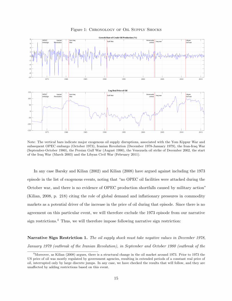
Figure 1: Chronology of Oil Supply Shocks

Growth Rate of Crude Oil Production (%)OPECembargo

IranianRevolution

Iran-IraqWar

Gulf WarVenezuela

unrestIraq war

Libyancivil war

1975 1980 1985 1990 1995 2000 2005 2010 2015-10

-8

-6

-4

-2

0

2

4

6

8

Log Real Price of Oil

OPECembargo

IranianRevolution

Iran-IraqWar

Gulf WarVenezuela

unrestIraq war

Libyancivil war

1975 1980 1985 1990 1995 2000 2005 2010 2015-150

-100

-50

0

50

100

150

Note: The vertical bars indicate major exogenous oil supply disruptions, associated with the Yom Kippur War andsubsequent OPEC embargo (October 1973), Iranian Revolution (December 1978-January 1979), the Iran-Iraq War(September-October 1980), the Persian Gulf War (August 1990), the Venezuela oil strike of December 2002, the startof the Iraq War (March 2003) and the Libyan Civil War (February 2011).

In any case Barsky and Kilian (2002) and Kilian (2008) have argued against including the 1973

episode in the list of exogenous events, noting that “no OPEC oil facilities were attacked during the

October war, and there is no evidence of OPEC production shortfalls caused by military action”

(Kilian, 2008, p. 218) citing the role of global demand and inflationary pressures in commodity

markets as a potential driver of the increase in the price of oil during that episode. Since there is no

agreement on this particular event, we will therefore exclude the 1973 episode from our narrative

sign restrictions.4 Thus, we will therefore impose following narrative sign restriction:

Narrative Sign Restriction 1. The oil supply shock must take negative values in December 1978,

January 1979 (outbreak of the Iranian Revolution), in September and October 1980 (outbreak of the

4Moreover, as Kilian (2008) argues, there is a structural change in the oil market around 1973. Prior to 1973 theUS price of oil was mostly regulated by government agencies, resulting in extended periods of a constant real price ofoil, interrupted only by large discrete jumps. In any case, we have checked the results that will follow, and they areunaffected by adding restrictions based on this event.

15

Iran-Iraq War), August 1990 (outbreak of the Persian Gulf War), December 2002 (Venezuela oil

strike), March 2003 (outbreak of the Iraq War) and February 2011 (outbreak of the Libyan Civil War).

It is also agreed that the oil supply shocks described in Restriction 1 “resulted in dra-

matic and immediate disruption of the flow of oil from key global producers” (Hamilton, 2009, p.

220). Therefore, we will use the following restriction:

Narrative Sign Restriction 2. For the periods specified by Restriction 1, oil supply

shocks are the most important contributor to the observed unexpected movements in oil production

growth. In other words, the absolute value of the contribution of oil supply shocks is larger than the

absolute contribution of any other structural shock.

While Restriction 2 reflects the agreement that the bulk of the unexpected fall in oil pro-

duction growth was due to negative oil supply shocks, there is much less agreement in the literature

about the ultimate cause of the unexpected increase in the real price of oil. For instance, while

Hamilton (2009), p. 224, argues that “oil price shocks of past decades were primarily caused by

significant disruptions in crude oil production brought about by largely exogenous geopolitical

events,” Lutz Kilian, in the comment to the same paper, expresses the view that “a growing body

of evidence argues against the notion that the earlier oil price shocks were driven primarily by

unexpected disruptions of the global supply of crude oil” (Kilian, 2009a, p. 268.), emphasizing

instead the role of the demand for oil. It is possible, however, to find an agreement that “for the

oil dates of 1980 and 1990/91 there is no evidence of aggregate demand pressures in industrial

commodity markets” (Kilian, 2008, p. 234.). Thus, although there is no agreement on whether

oil supply or oil demand shocks caused the unexpected changes in the real price of oil, it seems

that both Kilian (2008) and Hamilton (2009) agree that aggregate activity shocks were not

responsible for the increases observed in 1980 or 1990. Hence, we will also use the following restriction:

Narrative Sign Restriction 3. For the periods corresponding to September-October 1980

(outbreak of the Iran-Iraq War) and August 1990 (outbreak of the Persian Gulf War), aggregate

16

activity shocks are the least important contributor to the observed unexpected movements in the real

price of oil. In other words, the absolute value of the contribution of aggregate activity shocks is

smaller than the absolute contribution of any other structural shock.

Figure 2: IRFs with and without Narrative Sign Restrictions

Oil Production to Oil Supply Shock

0 4 8 12 16

-2

-1

0

1

Perc

ent

Economic Activity Index to Oil Supply Shock

0 4 8 12 16-5

0

5

10Real Oil Price to Oil Supply Shock

0 4 8 12 16-5

0

5

10

Oil Production to Aggregate Activity Shock

0 4 8 12 16

-2

-1

0

1

Perc

ent

Economic Activity Index to Aggregate Activity Shock

0 4 8 12 16-5

0

5

10Real Oil Price to Aggregate Activity Shock

0 4 8 12 16-5

0

5

10

Oil Production to Oil Demand Shock

0 4 8 12 16Months

-2

-1

0

1

Perc

ent

Economic Activity Index to Oil Demand Shock

0 4 8 12 16Months

-5

0

5

10Real Oil Price to Oil Demand Shock

0 4 8 12 16Months

-5

0

5

10

Note: The gray shaded area represents the 68% (point-wise) confidence bands for the IRFs, and the solid blue lines arethe median IRFs using the baseline identification restrictions. The pink shaded areas and red solid lines display theequivalent quantities when Restrictions 1-3 in Subsection 4.2 are also satisfied. Note that the IRF to oil productionhas been accumulated to the level.

In terms of the definitions in Section 3, Restriction 1 is a restriction on the signs of the

structural shocks, whereas Restrictions 2 and 3 are Type I restrictions on the historical decomposi-

tions of the data into structural shocks. Appendix A describes the functions F(Θ) and the matrices

Sj necessary to implement the baseline restriction and Restrictions 1-3.

4.3 Results

Figure 2 displays IRFs of the three variables to the three structural shocks, with and without the

narrative information. The gray shaded area represents the 68% (point-wise) confidence bands for

the IRFs and the solid blue line are the point-wise median IRFs using the baseline identification.

17

The pink shaded areas and red solid lines display the equivalent quantities when Restrictions 1-3

are also used. The narrative sign restrictions dramatically narrows down the uncertainty around

many of the IRFs relative to the baseline identification and modifies the shape of some of the IRFs

in economically meaningful ways. Oil demand shocks are shown to have a larger contemporaneous

effect on the real price of oil that dissipates after around 18 months, whereas aggregate activity

shocks have a small initial effect that gradually builds up over time. Some of the IRFs of the

economic activity index are also altered substantially. In particular, oil demand shocks have an

initial impact on real economic activity that is much smaller in absolute value than in the baseline

specification. Although it is negative at impact, it builds over time and becomes significant after

about 18 months. The response of real economic activity to aggregate activity shocks is stronger and

more persistent. The IRFs with the narrative sign restrictions are strikingly similar to the results

reported by Kilian (2009b) using the traditional Cholesky decomposition, with the major difference

that, in our identification scheme, oil demand shocks are contractionary for economic activity,

whereas in the recursive specification a positive oil demand shock, somewhat counter-intuitively,

caused a temporary boom in economic activity.5

The economic implications of Restrictions 1-3 become clear when examining the forecast error

variance decompositions (FEVD), which show what fraction of the unexpected fluctuations in the

variables at different horizons can be attributed to each structural shock. Figure 3 shows that when

the narrative information and the baseline identification are used, oil demand shocks are responsible

for the bulk of the high frequency unexpected variation in the real price of oil, whereas economic

activity shocks become the most important source of unexpected fluctuations only after three years.

With regard to the economic activity index, aggregate activity shocks are now responsible for most

of the unexpected fluctuations, although oil supply and oil demand shocks are jointly responsible for

over 10% of the unexpected variance in economic activity after ten years. These conclusions clearly

contrast with the FEVD obtained using only the baseline specification, in which oil demand shocks

account for about 40% of the unexpected variation in the economic activity index at all horizons

and aggregate activity shocks are responsible for the largest share of unexpected fluctuations in the

real price of oil even at high frequency. Another important message from Figure 3 is the reduction

5The results using the traditional Cholesky decomposition that we refer to can be seen in Figure 3, pp. 1061, inKilian (2009b).

18

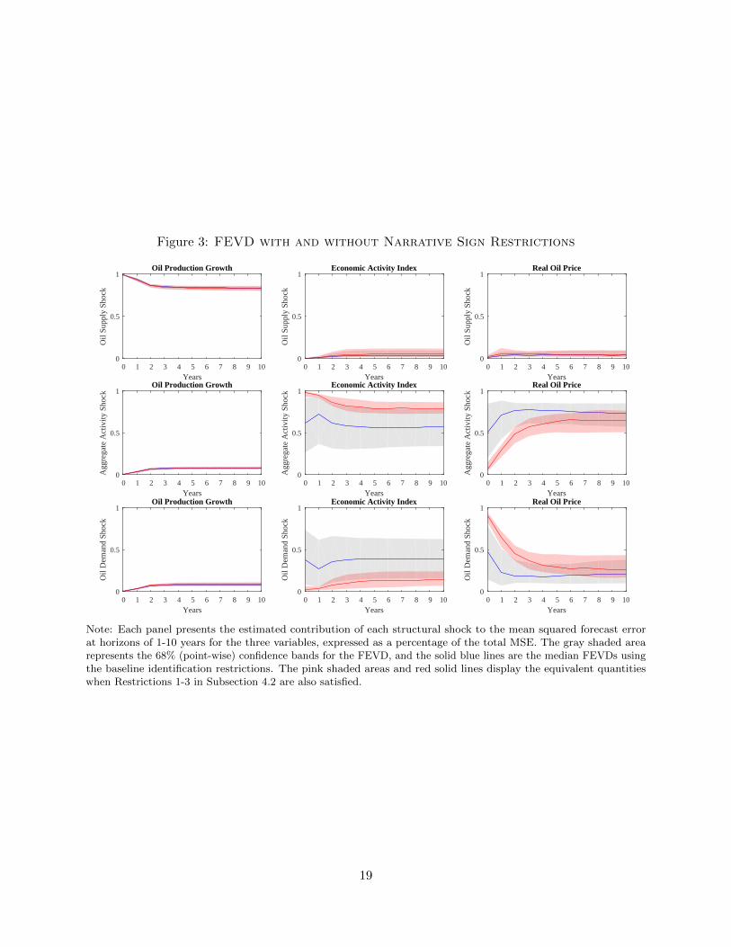
Figure 3: FEVD with and without Narrative Sign Restrictions

Oil Production Growth

0 1 2 3 4 5 6 7 8 9 10Years

0

0.5

1

Oil

Supp

ly S

hock

Economic Activity Index

0 1 2 3 4 5 6 7 8 9 10Years

0

0.5

1O

il Su

pply

Sho

ck

Real Oil Price

0 1 2 3 4 5 6 7 8 9 10Years

0

0.5

1

Oil

Supp

ly S

hock


0 1 2 3 4 5 6 7 8 9 10Years

0

0.5

1

Agg

rega

te A

ctiv

ity S

hock


0 1 2 3 4 5 6 7 8 9 10Years

0

0.5

1

Agg

rega

te A

ctiv

ity S

hock

Real Oil Price

0 1 2 3 4 5 6 7 8 9 10Years

0

0.5

1

Agg

rega

te A

ctiv

ity S

hock


0 1 2 3 4 5 6 7 8 9 10Years

0

0.5

1

Oil

Dem

and

Shoc

k


0 1 2 3 4 5 6 7 8 9 10Years

0

0.5

1

Oil

Dem

and

Shoc

k

Real Oil Price

0 1 2 3 4 5 6 7 8 9 10Years

0

0.5

1

Oil

Dem

and

Shoc

k

Note: Each panel presents the estimated contribution of each structural shock to the mean squared forecast errorat horizons of 1-10 years for the three variables, expressed as a percentage of the total MSE. The gray shaded arearepresents the 68% (point-wise) confidence bands for the FEVD, and the solid blue lines are the median FEVDs usingthe baseline identification restrictions. The pink shaded areas and red solid lines display the equivalent quantitieswhen Restrictions 1-3 in Subsection 4.2 are also satisfied.

19

in uncertainty around the median FEVD. If we compare the gray and the pink shaded areas we see

that adding the narrative sign restrictions (pink shaded areas) makes the 68% confidence bands

significantly smaller.

In our opinion, the results with narrative information are more plausible, since it appears to

us more realistic that the index of real economic activity is driven primarily by aggregate activity

shocks, i.e., other business cycle shocks not related to the oil market. Thus, after observing Figures

2 and 3, we can conclude that while the baseline specification, and in particular the restriction on

the price elasticity of supply, is very successful at sharpening the effects of oil supply shocks, the

narrative information dramatically helps disentangle the effects of aggregate activity and oil demand

shocks.

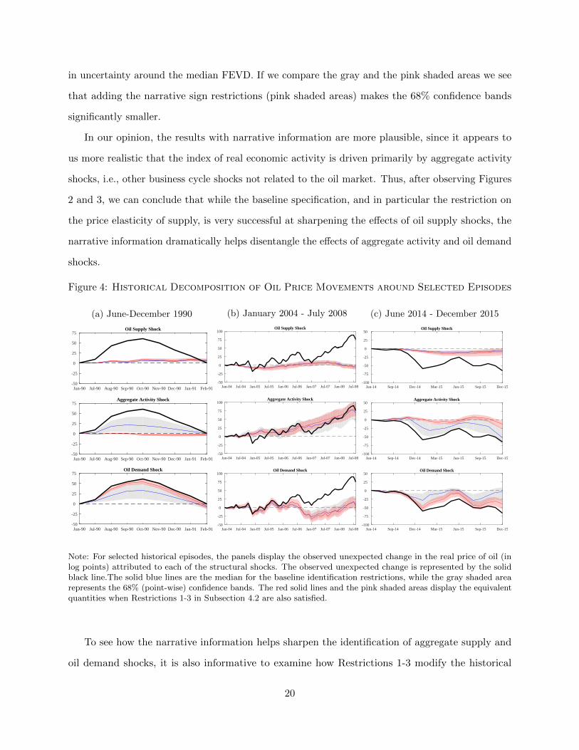
Figure 4: Historical Decomposition of Oil Price Movements around Selected Episodes

(a) June-December 1990

Oil Supply Shock

Jun-90 Jul-90 Aug-90 Sep-90 Oct-90 Nov-90 Dec-90 Jan-91 Feb-91-50

-25

0

25

50

75

Aggregate Activity Shock


-25

0

25

50

75

Oil Demand Shock


-25

0

25

50

75

(b) January 2004 - July 2008

Oil Supply Shock

Jan-04 Jul-04 Jan-05 Jul-05 Jan-06 Jul-06 Jan-07 Jul-07 Jan-08 Jul-08-50

-25

0

25

50

75

100



-25

0

25

50

75

100

Oil Demand Shock


-25

0

25

50

75

100

(c) June 2014 - December 2015

Oil Supply Shock

Jun-14 Sep-14 Dec-14 Mar-15 Jun-15 Sep-15 Dec-15-100

-75

-50

-25

0

25

50



-75

-50

-25

0

25

50

Oil Demand Shock


-75

-50

-25

0

25

50

Note: For selected historical episodes, the panels display the observed unexpected change in the real price of oil (inlog points) attributed to each of the structural shocks. The observed unexpected change is represented by the solidblack line.The solid blue lines are the median for the baseline identification restrictions, while the gray shaded arearepresents the 68% (point-wise) confidence bands. The red solid lines and the pink shaded areas display the equivalentquantities when Restrictions 1-3 in Subsection 4.2 are also satisfied.

To see how the narrative information helps sharpen the identification of aggregate supply and

oil demand shocks, it is also informative to examine how Restrictions 1-3 modify the historical

20

decomposition of the real price of oil for particular historical episodes. Panel (a) of Figure 4 looks

at the Persian Gulf War, which was one of the events included in Restrictions 1-3. The baseline

identification (gray shaded area) is consistent with many structural parameters that imply that

aggregate activity shocks were important contributors to the unexpected increase in log real oil

prices observed between July and November 1990. Including Restrictions 1-3 (pink shaded area)

reinforces the view of Kilian (2009b) and Kilian and Murphy (2014) that speculation in the physical

market, i.e., an oil demand shock, was the cause of the bulk of the unexpected 60% increase in the

real price of oil at the outbreak of the war. Panels (b) and (c) look at two events for which no

restrictions are imposed. For the run-up in the real price of oil between 2004-2008, displayed in

Panel (b), the narrative information agrees with the baseline identification in that aggregate activity

shocks were the main cause. This is in line with the results of the previous literature. For the 60%

unexpected decline in the real price of oil observed between July 2014 and December 2015, Panel

(c) shows how the baseline identification concludes that it was not due to oil supply shocks, but

leads to substantial uncertainty about whether aggregate activity shocks or oil demand shocks were

behind the collapse. With the narrative information the results clearly point toward oil demand

shocks as the source of the collapse.

4.4 Assessing the importance of each historical event

Because we focus on a small number of historical events, it is straightforward to assess the importance

of each of them. Table 2 computes what percentage of draws of the structural parameters that

satisfy the baseline specification violates each of the narrative sign restrictions, both individually and

jointly. The results indicate that Restrictions 1 and 2 are less relevant than Restriction 3. However,

it is noteworthy that the baseline identification still includes many structural parameters for which

a positive supply shock occurred during either the 1979 Iranian Revolution or the 2003 Iraq War,

contradicting Restriction 1. In total, 42% of the structural parameters that satisfy the baseline

specification violate Restriction 1. It is also the case that over 20% of the structural parameters

that satisfy the baseline specification do not satisfy Restriction 2 for the 1979 Iranian Revolution or

the 2003 Iraq War. But it is clear that Restriction 3 is key to obtaining the results of Figures 2 and

3, given that in total 93% of the structural parameters that satisfy the baseline specification do not

21

respect Restriction 3.

Table 2: Probability of Violating the Narrative Sign Restrictions

Restr. 1 Restr. 2 Restr. 3 Any Restr.

Iranian Revolution 20% 2.9% − 21%Iran-Iraq War 0% 0% 46% 46%Gulf War 0% 0% 93% 93%Venezuela Unrest 0% 0% − 0%Iraq War 43% 21% − 53%Libyan Civil War 4.6% 1% − 5%Any Episodes 42% 24% 93% 98%

In fact, it turns out that to obtain the results of Figures 2 and 3 it is sufficient to impose

Restriction 3 for the August 1990 event. In other words, one only needs to agree that expansionary

aggregate activity shocks were the least important contributor to the unexpected spike in the real

price of oil observed that month, a view that has been described as agreeable to a wide group of

experts (Kilian and Murphy, 2014, p. 468), to obtain our results. To see this more clearly, we can

consider Alternative Restriction 3:

Alternative Restriction 3. For the period corresponding to August 1990 (outbreak of

the Persian Gulf War), aggregate activity shocks are the least important contributor to the observed

unexpected movements in the real price of oil. In other words, the absolute value of the contribu-

tion of aggregate activity shocks is smaller than the absolute contribution of any other structural shock.

Figure 5 plots the same IRFs reported in Figure 2, but the pink shaded areas and red solid

lines now use exclusively Alternative Restriction 3 instead of Restrictions 1-3.6 As the reader

can see, Figures 2 and 5 are almost identical. Hence using either Restrictions 1-3 or Alternative

Restriction 3 has comparable effects on the IRFs and on other results such as the FEVD and

historical decompositions presented above.7 Given that the challenge is to come up with additional

6Alternatively, one may also reformulate Restrictions 1 and 2 so as to include only the August 1990 event, but ascan be seen from the third row of Table 2, Restrictions 1 and 2 are always satisfied by the baseline specification forthis particular event. Therefore it is enough to use just Alternative Restriction 3.

7The equivalents to Figures 3 and 4 using exclusively Alternative Restriction 3 are essentially identical to the

22


(Alternative Restriction 3)

Oil Production Growth to Oil Supply Shock

0 4 8 12 16

Perc

ent

-2

-1

0

1


0 4 8 12 16-5

0

5


0 4 8 12 16-5

0

5

10

Oil Production Growth to Aggregate Activity Shock

0 4 8 12 16

Perc

ent

-2

-1

0

1


0 4 8 12 16-5

0

5


0 4 8 12 16-5

0

5

10

Oil Production Growth to Oil Demand Shock

Months 0 4 8 12 16

Perc

ent

-2

-1

0

1


Months 0 4 8 12 16

-5

0

5


Months 0 4 8 12 16

-5

0

5

10

Note: The gray shaded area represents the 68% (point-wise) confidence bands for the IRFs, and the solid blue linesare the median IRFs using the baseline identification restrictions. The pink shaded areas and red solid lines displaythe equivalent quantities when Alternative Restriction 3 is also satisfied. Note that the IRF to oil production hasbeen accumulated to the level.

uncontentious sign restrictions that help shrink the set of admissible structural parameters, the

resemblance of the results using either Restrictions 1-3 or Alternative Restriction 3 is a great success.

By using a single narrative sign restriction to constraint the set of structural parameters to those

whose implied behavior in August 1990 agrees with the generally accepted description of that event,

we can greatly sharpen the separate identification of aggregate activity and oil demand shocks for

the entire sample, including many other periods for which narrative information is not available.

Given that the restriction relating to August 1990 appears to be key to our results, it warrants

some additional discussion. In particular, we will analyze the robustness of the results to using the

Type II variant of Alternative Restriction 3, instead of the Type I variant we have been using so far.

Recall from Section 3.4 that for this case the Type I restriction specifies that the contribution of

the aggregate demand shock to the spike in the real price of oil is “less important than any other,”

originals, which use Restrictions 1-3. We do not display them owing to space considerations, but they are availableupon request.

23

whereas the Type II restriction would specify that the contribution is “less important than the sum of

all others.” Clearly, in this case Type I is a stronger version than Type II, since being less important

than any other contribution automatically implies being less important than the (absolute) sum of

all others (see the discussion in Section 3.4.3). Figure 6 plots the same IRFs reported in Figure 5

when exclusively using Alternative Restriction 3, but in its milder Type II variant. As the reader

can see, the main conclusions are maintained. In any case, since it seems accepted that aggregate

activity shocks are the least important contributor to the observed unexpected movements in the

real price of oil in August 1990, we support the view that the more restrictive Type I variant is

adequate. However, changing from Type I and Type II can be a useful way of expressing different

degrees of confidence in the narrative information itself.

4.5 Final remarks on demand and supply shocks in the oil market

To sum up, we have shown that, while the identification scheme proposed by Kilian and Murphy

(2012) does a very good job of distinguishing the effects of supply and demand shocks, the narrative

sign restrictions are very successful in sharpening the inference about the structural shocks that

drive the oil market. Using Kilian (2008) and Hamilton (2009) as sources, we obtain a list of

post-1973 historical events that generate a number of uncontroversial narrative sign restrictions

that allow us to distinguish between aggregate activity and oil demand shocks. In fact, it turns out

that a single narrative sign restriction that ensures that the structural parameters are in line with

the established narrative about the outbreak of the Persian Gulf War, whether in its stronger or

milder variant, is enough to separate the effects of these two shocks. The fact that a single sign

narrative restriction is enough is very important given that we started this section with a query

for few uncontroversial sign restrictions that may help us reduce the set of structural parameters

consistent with the baseline identification.

24

Figure 6: IRFs with and without Sign Narrative Restrictions

(Alternative Restriction 3 – Type II)

Oil Production Growth to Oil Supply Shock

0 4 8 12 16

Perc

ent

-2

-1

0

1


0 4 8 12 16-5

0

5


0 4 8 12 16-5

0

5

10

Oil Production Growth to Aggregate Activity Shock

0 4 8 12 16

Perc

ent

-2

-1

0

1


0 4 8 12 16-5

0

5


0 4 8 12 16-5

0

5

10

Oil Production Growth to Oil Demand Shock

Months 0 4 8 12 16

Perc

ent

-2

-1

0

1


Months 0 4 8 12 16

-5

0

5


Months 0 4 8 12 16

-5

0

5

10

Note: The gray shaded area represents the 68% (point-wise) confidence bands for the IRFs and the solid blue linesare the median IRFs using the baseline identification restrictions. The pink shaded areas and red solid lines displaythe equivalent quantities when the Alternative Restriction 3 (Type II) is also satisfied. Note that the IRF to oilproduction has been accumulated to the level.

5 Monetary Policy Shocks and the Volcker Reform

An extensive literature has studied the effect of monetary policy shocks on output using SVARs,

identified with traditional zero restrictions, as in Christiano et al. (1999), Bernanke and Mihov

(1998), sign restrictions, as in Uhlig (2005), or both, as in Arias et al. (2016a). SVARs identified

using traditional zero restrictions have consistently found that an exogenous increase in the fed

funds rate induces a reduction in real activity. This intuitive result has become the “consensus.”

This consensus view, however, has been challenged by Uhlig (2005), who criticizes the traditional

SVAR approach for imposing a questionable zero restriction on the IRF of output to a monetary

policy shock on impact. To solve the problem he proposes to identify a shock to monetary policy by

imposing sign restrictions only on the IRFs of prices and nonborrowed reserves to this shock, while

imposing no restrictions on the IRF of output. The lack of restrictions on the IRF of output to a

25

monetary policy shock makes this is an attractive approach. Importantly, under his identification,

the “consensus” vanishes; an exogenous increase in the fed funds rate does not necessarily induce a

reduction in real activity.

An alternative approach uses historical sources to isolate events that constitute exogenous

monetary policy shocks. Following the pioneering work of Friedman and Schwartz (1963), Romer

and Romer (1989) combed through the minutes of the FOMC to create a dummy time series of

events that they argued represented exogenous tightenings of monetary policy. Focusing exclusively

on contractionary shocks, they singled out a handful of episodes in the postwar period “in which

the Federal Reserve attempted to exert a contractionary influence on the economy in order to

reduce inflation” (Romer and Romer (1989) , p. 134). The Romers’ monetary policy time series

narrative became very influential, but has been criticized by Leeper (1997) who pointed out that

their dates are predictable from past macroeconomic data. As a consequence, in recent years

alternative methods have been developed to construct time series of monetary policy shocks that

are by design exogenous to the information set available at the time of the policy decision. The first

prominent example is Romer and Romer (2004), who regressed changes of the intended federal funds

rate between FOMC meetings on changes in the Fed’s Greenbook forecasts of output and inflation.

By construction, the residuals from this regression are orthogonal to all the information contained

in the Greenbook forecasts, and can plausibly taken to be a measure of exogenous monetary policy

shocks. A second approach looks at high-frequency financial data. Kuttner (2001), and Gurkaynak

et al. (2005), among others, look at movements in federal funds futures contracts during a short

window around the time of policy announcements to isolate the monetary policy shocks.

However, the existing narrative time series are sometimes inconclusive and others contradictory.

This is not just due to differences in methods and sources, but, as Ramey (2016) recently pointed

out, to the fact that the Federal Reserve has historically reacted in a systematic way to output and

inflation developments (see also Leeper et al., 1996). This systematic response is a key difference

with the oil supply shocks analyzed in Section 4, so the occurrence and importance of truly exogenous

monetary policy shocks remain controversial. Thus, monetary policy shocks are much more difficult

to isolate than oil supply shocks.

For this reason, in this section we will use narrative sign restrictions for a single event: October of

26

1979. The monetary policy decisions of October 6, 1979, enacted shortly after Paul Volcker became

chairman of the Fed, are described by Romer and Romer (1989) as “a major anti-inflationary shock to

monetary policy” and represent, in our view, the clearest case in the postwar period of an exogenous

monetary policy shock. Lindsey et al. (2013) provide a detailed account of the events leading to the

decision to abandon targeting the Federal Funds rate in favor of targeting non-borrowed reserves

as the operating procedure for controlling the money supply. While macroeconomic conditions, in

particular, the deterioration of the inflation outlook and the increase in the real price of oil that

followed the Iranian Revolution of 1978-79, played a large role in causing the shift, the forcefulness

and the surprise character of the action and the dramatic break with established practice in the

conduct of policy strongly suggest the occurrence of a monetary policy shock.

As we will see, once we add to Uhlig’s (2005) identification narrative sign restrictions so that

only structural parameters that imply an important negative monetary policy shock occurred in

October of 1979 are permitted, the “consensus” revives. Given that the challenge is to come up

with few additional uncontentious sign restrictions that help shrink the set of admissible structural

parameters, the fact that the “consensus” is recovered by just considering narrative information

about a single event is a great achievement. By constraining the structural parameters so that

an important negative monetary policy shock occurred during October of 1979, we can reconcile

Uhlig’s (2005) critique with the “consensus”.

5.1 Data and Baseline Specification

Our starting point is the reduced-form VAR used among others by Christiano et al. (1999), Bernanke

and Mihov (1998) and Uhlig (2005). The model includes six variables: real output, the GDP deflator,

a commodity price index, total reserves, nonborrowed reserves, and the federal funds rate. As in the

previous section, to maximize comparability with previous work we chose the exact specification,

reduced-form prior and data definitions used in the aforementioned papers. Our sample period is

January 1965 to November 2007.8 Our baseline identification is identical to Uhlig (2005). Specifically,

8The VAR is estimated on monthly data using 12 lags, no constant or deterministic trends, and uninformativepriors. We refer to the aforementioned papers for details on the sources and the model specification. Following Ariaset al. (2016a), we stop the sample in November 2007 because starting in December 2007 there are large movements inreserves associated with the global financial crisis. Furthermore, the federal funds rate has been at the zero lowerbound since November 2008. Including the post-crisis sample could obscure the comparison with the results of earlier

27

he postulates that a monetary policy shock has the effects given in Table 3 for the first six months.

Table 3: Sign Restrictions on Responses at Horizons 0 to 5

Monetary Policy Shock

Real GDPGDP Deflator −Commodity Price Index −Total Reserves −Nonborrowed Reserves −Federal Funds Rate +

5.2 The narrative information

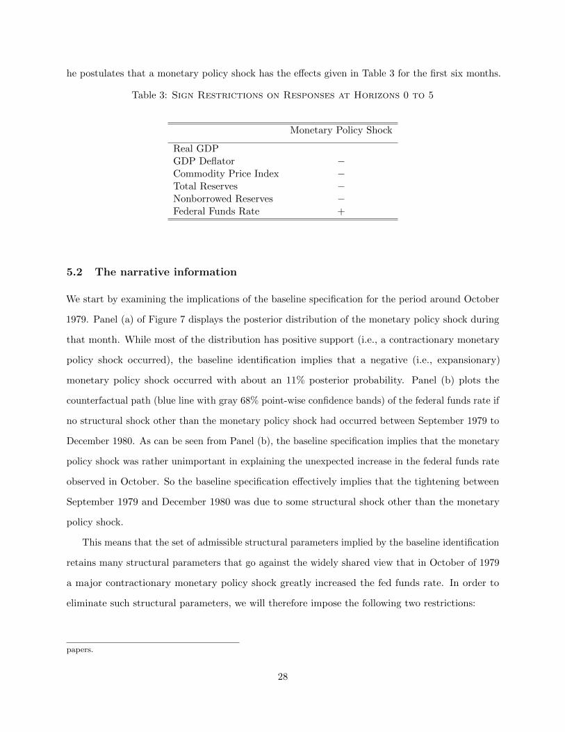
We start by examining the implications of the baseline specification for the period around October

1979. Panel (a) of Figure 7 displays the posterior distribution of the monetary policy shock during

that month. While most of the distribution has positive support (i.e., a contractionary monetary

policy shock occurred), the baseline identification implies that a negative (i.e., expansionary)

monetary policy shock occurred with about an 11% posterior probability. Panel (b) plots the

counterfactual path (blue line with gray 68% point-wise confidence bands) of the federal funds rate if

no structural shock other than the monetary policy shock had occurred between September 1979 to

December 1980. As can be seen from Panel (b), the baseline specification implies that the monetary

policy shock was rather unimportant in explaining the unexpected increase in the federal funds rate

observed in October. So the baseline specification effectively implies that the tightening between

September 1979 and December 1980 was due to some structural shock other than the monetary

policy shock.

This means that the set of admissible structural parameters implied by the baseline identification

retains many structural parameters that go against the widely shared view that in October of 1979

a major contractionary monetary policy shock greatly increased the fed funds rate. In order to

eliminate such structural parameters, we will therefore impose the following two restrictions:

papers.

28

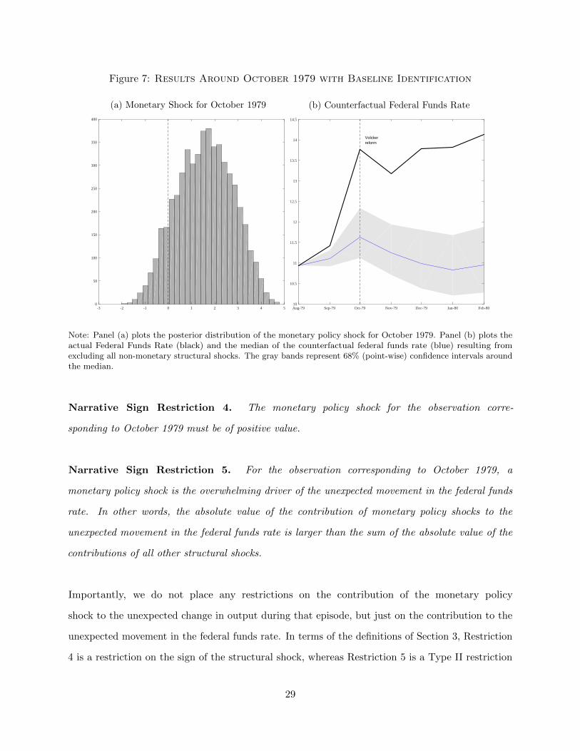
Figure 7: Results Around October 1979 with Baseline Identification

(a) Monetary Shock for October 1979

-3 -2 -1 0 1 2 3 4 50

50

100

150

200

250

300

350

400

(b) Counterfactual Federal Funds Rate

Volckerreform

Aug-79 Sep-79 Oct-79 Nov-79 Dec-79 Jan-80 Feb-8010

10.5

11

11.5

12

12.5

13

13.5

14

14.5

Note: Panel (a) plots the posterior distribution of the monetary policy shock for October 1979. Panel (b) plots theactual Federal Funds Rate (black) and the median of the counterfactual federal funds rate (blue) resulting fromexcluding all non-monetary structural shocks. The gray bands represent 68% (point-wise) confidence intervals aroundthe median.

Narrative Sign Restriction 4. The monetary policy shock for the observation corre-

sponding to October 1979 must be of positive value.

Narrative Sign Restriction 5. For the observation corresponding to October 1979, a

monetary policy shock is the overwhelming driver of the unexpected movement in the federal funds

rate. In other words, the absolute value of the contribution of monetary policy shocks to the

unexpected movement in the federal funds rate is larger than the sum of the absolute value of the

contributions of all other structural shocks.

Importantly, we do not place any restrictions on the contribution of the monetary policy

shock to the unexpected change in output during that episode, but just on the contribution to the

unexpected movement in the federal funds rate. In terms of the definitions of Section 3, Restriction

4 is a restriction on the sign of the structural shock, whereas Restriction 5 is a Type II restriction

29

on the historical decomposition of the fed funds rate into structural shocks. Appendix B describes

the functions F(Θ) and the matrices Sj necessary to implement the baseline restrictions and

Restrictions 4 and 5.

Note that the specified Type II restriction postulates that the absolute value of the contribution

of the monetary policy shock is “larger than the sum of the absolute value of the contribution of all

other structural shocks” to the the unexpected movement in the federal funds rate in October 1979,

whereas a Type I restriction would postulate that the contribution is “larger than the absolute

value of the contribution of any other structural shocks.” Clearly, in this case Type II is a stronger

version than Type I. In our view, there is overwhelming evidence that the unexpected increase in

the federal funds rate observed in October 1979 was the outcome of a monetary policy shock; hence,

a Type II restriction is justified. Nevertheless, we will check the robustness of our results to speci-

fying a milder Type I version of this restriction. To do this we will consider Alternative Restriction 5:

Alternative Restriction 5. For the observation corresponding to October 1979, a mone-

tary policy shock is the most important driver of the unexpected movement in the federal funds rate.

In other words, the absolute value of the contribution of monetary policy shocks to the unexpected

movement in the federal funds rate is larger than the absolute value of the contribution of any other

structural shock.

5.3 Results

Figure 8 compares the IRFs to a monetary policy shock, with and without narrative sign restrictions.

The gray shaded area represents the 68% (point-wise) confidence bands for the IRFs and the solid

blue lines are the median IRFs using the baseline identification. These results replicate the IRFs

depicted in Figure 6 of Uhlig (2005). The pink shaded areas and red solid lines display the equivalent

quantities when Restrictions 4 and 5 are also used. As one can observe, the inclusion of Restrictions

4 and 5 is enough to recover the “consensus.” The results reported highlight that the narrative

information embedded in a single event can shrink the set of admissible structural parameters so

dramatically that the economic implications change. In this case, the inclusion of a single event

changes the sign of the effect of monetary policy shocks on output.

30


Output

0 1 2 3 4 5

Perc

ent

-0.3

-0.2

-0.1

0

0.1

0.2

0.3

0.4GDP Deflator

0 1 2 3 4 5

Perc

ent

-0.8

-0.7

-0.6

-0.5

-0.4

-0.3

-0.2

-0.1

0Commodity Prices

0 1 2 3 4 5

Perc

ent

-4

-3.5

-3

-2.5

-2

-1.5

-1

-0.5

0

Total Reserves

Years0 1 2 3 4 5

Perc

ent

-2

-1.5

-1

-0.5

0

0.5Non-Borrowed Res.

Years0 1 2 3 4 5

Perc

ent

-2

-1.5

-1

-0.5

0

0.5Fed Funds Rate

Years0 1 2 3 4 5

Bas

is p

oint

s

-25

0

25

50

Note: The gray shaded area represents the 68% (point-wise) confidence bands for the IRFs, and the solid blue linesare the median IRFs using the baseline identification restrictions. The pink shaded areas and red solid lines displaythe equivalent quantities for the models that additionally satisfy Restrictions 4 and 5 in Subsection 5.2. The IRFshave been normalized so that the monetary policy shock has an impact of 25 basis points on the Federal Funds rate.

How do Restrictions 4 and 5 change the implications for the period around October 1979? Figure

9 plots the same results displayed in Figure 7, but this time with the narrative sign restrictions

in place. Panel (a) of Figure 9 displays the posterior distribution of the monetary policy shock

during that month when Restrictions 4 and 5 are also used. The distribution of the structural

shock has now positive support with 100% probability. Panel (b) plots the counterfactual path (red

line with pink 68% point-wise confidence bands) of the federal funds rate if no structural shock

other than the monetary policy shock had occurred between September 1979 and December 1980.

The monetary policy shock was the overwhelming contributor to the unexpected increase in the

federal funds rate. The figure tells us that the monetary policy shock was very large (between 2

and 5 standard deviations) and that it was responsible for between 100 and 150 basis points of the

roughly 225-basis-point unexpected increase in the federal funds rate observed in October 1979. It

is important to emphasize that these magnitudes are not imposed by Restrictions 4 and 5; only the

sign of the shock and the sign of the contribution of the monetary policy shock relative to other

structural shocks are.

31

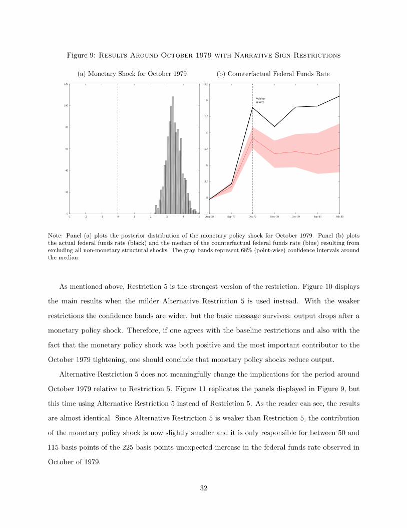
Figure 9: Results Around October 1979 with Narrative Sign Restrictions


-3 -2 -1 0 1 2 3 4 50

20

40

60

80

100

120


Volckerreform

Aug-79 Sep-79 Oct-79 Nov-79 Dec-79 Jan-80 Feb-8010.5

11

11.5

12

12.5

13

13.5

14

14.5

Note: Panel (a) plots the posterior distribution of the monetary policy shock for October 1979. Panel (b) plotsthe actual federal funds rate (black) and the median of the counterfactual federal funds rate (blue) resulting fromexcluding all non-monetary structural shocks. The gray bands represent 68% (point-wise) confidence intervals aroundthe median.

As mentioned above, Restriction 5 is the strongest version of the restriction. Figure 10 displays

the main results when the milder Alternative Restriction 5 is used instead. With the weaker

restrictions the confidence bands are wider, but the basic message survives: output drops after a

monetary policy shock. Therefore, if one agrees with the baseline restrictions and also with the

fact that the monetary policy shock was both positive and the most important contributor to the

October 1979 tightening, one should conclude that monetary policy shocks reduce output.

Alternative Restriction 5 does not meaningfully change the implications for the period around

October 1979 relative to Restriction 5. Figure 11 replicates the panels displayed in Figure 9, but

this time using Alternative Restriction 5 instead of Restriction 5. As the reader can see, the results

are almost identical. Since Alternative Restriction 5 is weaker than Restriction 5, the contribution

of the monetary policy shock is now slightly smaller and it is only responsible for between 50 and

115 basis points of the 225-basis-points unexpected increase in the federal funds rate observed in

October of 1979.

32


(Restriction 4 and Alternative Restriction 5)

Output

0 1 2 3 4 5

Perc

ent

-0.3

-0.2

-0.1

0

0.1

0.2

0.3

0.4GDP Deflator

0 1 2 3 4 5

Perc

ent

-0.8

-0.7

-0.6

-0.5

-0.4

-0.3

-0.2

-0.1

0Commodity Prices

0 1 2 3 4 5

Perc

ent

-4

-3.5

-3

-2.5

-2

-1.5

-1

-0.5

0

Total Reserves

Years0 1 2 3 4 5

Perc

ent

-2

-1.5

-1

-0.5

0


Years0 1 2 3 4 5

Perc

ent

-2

-1.5

-1

-0.5

0

0.5Fed Funds Rate

Years0 1 2 3 4 5

Bas

is p

oint

s

-25

0

25

50

Note: The gray shaded area represents the 68% (point-wise) confidence bands for the IRFs, and the solid blue lines arethe median IRFs using the baseline identification restrictions. The pink shaded areas and red solid lines display theequivalent quantities for the models that additionally satisfy Restriction 4 and Alternative Restriction 5 in Subsection5.2. The IRFs have been normalized so that the monetary policy shock has an impact of 25 basis points on the federalfunds rate.

5.4 Including additional events: a new chronology

The results above have highlighted that using narrative information for a single event − October

1979 − is enough to recover the “consensus” around the effect of monetary policy shocks on output.

That event is in our view the clearest and most uncontroversial example of a monetary policy shock,

but as mentioned above, there is a long literature that uses historical sources to isolate monetary

policy shocks. In Appendix C, we survey this literature and drawing, in particular, on Romer and

Romer (1989), Romer and Romer (2004), and Gurkaynak et al. (2005), identify eight events for

which there appears to be reasonable agreement that a monetary policy shock occurred. Of these,

four − April 1974, October 1979, December 1988 and February 1994 − were contractionary shocks

and four − December 1990, October 1998, April 2001, and November 2002 − were expansionary

shocks. The inclusion of narrative information for all these events leads to results very similar

to those reported above using only October 1979 but, as expected, the confidence bands narrow

33

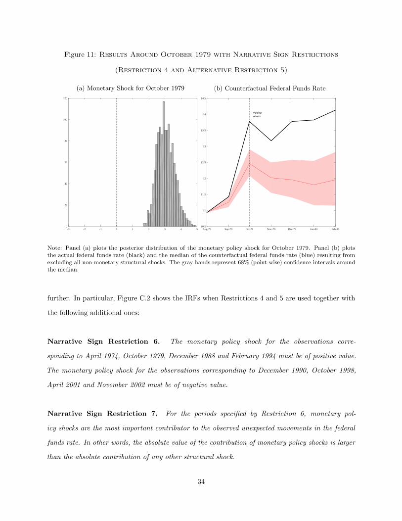
Figure 11: Results Around October 1979 with Narrative Sign Restrictions

(Restriction 4 and Alternative Restriction 5)


-3 -2 -1 0 1 2 3 4 50

20

40

60

80

100

120


Volckerreform

Aug-79 Sep-79 Oct-79 Nov-79 Dec-79 Jan-80 Feb-8010.5

11

11.5

12

12.5

13

13.5

14

14.5

Note: Panel (a) plots the posterior distribution of the monetary policy shock for October 1979. Panel (b) plotsthe actual federal funds rate (black) and the median of the counterfactual federal funds rate (blue) resulting fromexcluding all non-monetary structural shocks. The gray bands represent 68% (point-wise) confidence intervals aroundthe median.

further. In particular, Figure C.2 shows the IRFs when Restrictions 4 and 5 are used together with

the following additional ones:

Narrative Sign Restriction 6. The monetary policy shock for the observations corre-

sponding to April 1974, October 1979, December 1988 and February 1994 must be of positive value.

The monetary policy shock for the observations corresponding to December 1990, October 1998,

April 2001 and November 2002 must be of negative value.

Narrative Sign Restriction 7. For the periods specified by Restriction 6, monetary pol-

icy shocks are the most important contributor to the observed unexpected movements in the federal

funds rate. In other words, the absolute value of the contribution of monetary policy shocks is larger

than the absolute contribution of any other structural shock.

34

Restriction 6 is equivalent to Restriction 4, while Restriction 7 is equivalent to Alterna-

tive Restriction 5 for the additional dates. This implies that we impose only the weaker Type I

restriction for all events other than the Volcker Reform. As mentioned above, this is because the

Volcker Reform is the clearest episode.

Finally, we also would like to mention that while the restrictions relating to the Volcker Reform

are sufficient to recover the “consensus,” they are not necessary. It is possible to obtain results

similar to the ones reported in Figures 8 and 10 by just imposing Restrictions 4 and 5 or Restriction

4 and Alternative Restriction 5 only for the 1998, 1994 or 2001 dates on their own.9

6 Conclusion

Historical sources have long been regarded as useful for identifying structural shocks. In this paper,

we have shown how to use narrative sign restrictions to identify SVARs. We place sign restrictions on

structural shocks and the historical decomposition of the data at certain historical periods, ensuring

that the structural parameters are consistent with the established account of these episodes. We

have illustrated our approach with the case of oil and monetary shocks. We have shown that a small

number of narrative sign restrictions related to key historical events, and sometimes even a single

event, can dramatically sharpen the inference or even alter the conclusions of SVARs identified

with the widespread practice of placing sign restrictions only on the IRFs. Relative to existing

narrative information methods, our approach has the advantage of requiring that we trust only

the sign and the relative importance of the structural shock for a small number of events, which

facilitates the practice of basing inference on a few uncontroversial sign restrictions on which the

majority of researchers agree and which lead to robust conclusions.

References

Arias, J. E., D. Caldara, and J. F. Rubio-Ramirez (2016a): “The Systematic Component

of Monetary Policy in SVARs: An Agnostic Identification Procedure,” International Finance

9These additional figures are available upon request.

35

Discussion Papers 1131, Board of Governors of the Federal Reserve System (U.S.).

Arias, J. E., J. F. Rubio-Ramirez, and D. F. Waggoner (2016b): “Inference Based on SVARs

Identified with Sign and Zero Restrictions: Theory and Applications,” Working paper, Federal

Reserve Bank of Atlanta.

Barsky, R. B. and L. Kilian (2002): “Do We Really Know that Oil Caused the Great Stagflation?

A Monetary Alternative,” in NBER Macroeconomics Annual 2001, Volume 16, National Bureau

of Economic Research, Inc, NBER Chapters, 137–198.

Baumeister, C. and J. D. Hamilton (2015): “Structural Interpretation of Vector Autoregressions

with Incomplete Identification: Revisiting the Role of Oil Supply and Demand Shocks,” Mimeo.

Baumeister, C. and G. Peersman (2013): “The role of timevarying price elasticities in accounting

for volatility changes in the crude oil market,” Journal of Applied Econometrics, 28, 1087–1109.

Bernanke, B. S. and I. Mihov (1998): “Measuring Monetary Policy,” The Quarterly Journal of

Economics, 113, 869–902.

Caldara, D. and E. Herbst (2016): “Monetary Policy, Real Activity, and Credit Spreads:

Evidence from Bayesian Proxy SVAR,” FEDs Working Paper Series 2016-049, Board of Governors

of the Federal Reserve System (U.S.).

Canova, F. and G. D. Nicolo (2002): “Monetary disturbances matter for business fluctuations

in the G-7,” Journal of Monetary Economics, 49, 1131–1159.

Christiano, L. J., M. Eichenbaum, and C. L. Evans (1999): “Monetary policy shocks: What

have we learned and to what end?” in Handbook of Macroeconomics, ed. by J. B. Taylor and

M. Woodford, Elsevier, vol. 1 of Handbook of Macroeconomics, chap. 2, 65–148.

Drautzburg, T. (2016): “A Narrative Approach to a Fiscal DSGE Model,” Working paper 16-11,

Federal Reserve Bank of Philadelphia.

Faust, J. (1998): “The robustness of identified VAR conclusions about money,” International

Finance Discussion Papers 610, Board of Governors of the Federal Reserve System (U.S.).

36

Friedman, M. and A. Schwartz (1963): A Monetary History of the United States, 1867-1960,

National Bureau of Economic Research, Inc.

Gertler, M. and P. Karadi (2015): “Monetary Policy Surprises, Credit Costs, and Economic

Activity,” American Economic Journal: Macroeconomics, 7, 44–76.

Gurkaynak, R. S., B. Sack, and E. Swanson (2005): “Do Actions Speak Louder Than Words?

The Response of Asset Prices to Monetary Policy Actions and Statements,” International Journal

of Central Banking, 1.

Hamilton, J. D. (1985): “Historical Causes of Postwar Oil Shocks and Recessions,” The Energy

Journal, 0, 97–116.

——— (2009): “Causes and Consequences of the Oil Shock of 2007-08,” Brookings Papers on

Economic Activity, 40, 215–283.

Hoover, K. D. and S. J. Perez (1994): “Post hoc ergo propter hoc once more: an evaluation of

’does monetary policy matter?’ in the spirit of James Tobin,” Journal of Monetary Economics,

34, 47–74.

Juvenal, L. and I. Petrella (2015): “Speculation in the oil market,” Journal of Applied

Econometrics, 30, 621–649.

Kilian, L. (2008): “Exogenous Oil Supply Shocks: How Big Are They and How Much Do They

Matter for the U.S. Economy?” The Review of Economics and Statistics, 90, 216–240.

——— (2009a): “Comment,” in Causes and Consequences of the Oil Shock of 2007-08, ed. by

J. Hamilton, vol. 40, 215–283.

——— (2009b): “Not All Oil Price Shocks Are Alike: Disentangling Demand and Supply Shocks in

the Crude Oil Market,” American Economic Review, 99, 1053–69.

Kilian, L. and D. P. Murphy (2012): “Why agnostic sign restrictions are not enough: Un-

derstanding the Dynamics of Oil Market VAR Models,” Journal of the European Economic

Association, 10, 1166–1188.

37

——— (2014): “The Role of Inventories and Speculative Trading in the Global Market for Crude

Oil,” Journal of Applied Econometrics, 29, 454–478.

Kuttner, K. N. (2001): “Monetary policy surprises and interest rates: Evidence from the Fed

funds futures market,” Journal of Monetary Economics, 47, 523–544.

Leeper, E. M. (1997): “Narrative and VAR approaches to monetary policy: Common identification

problems,” Journal of Monetary Economics, 40, 641–657.

Leeper, E. M., C. A. Sims, and T. Zha (1996): “What does monetary policy do?” Brookings

Papers on Economic Activity, 1996, 1–78.

Lindsey, D. E., A. Orphanides, and R. H. Rasche (2013): “The Reform of October 1979:

How It Happened and Why,” Federal Reserve Bank of St. Louis Review, 487–542.

Mertens, K. and M. O. Ravn (2013): “The Dynamic Effects of Personal and Corporate Income

Tax Changes in the United States,” American Economic Review, 103, 1212–47.

Montiel-Olea, J. L., J. H. Stock, and M. W. Watson (2015): “Uniform Inference in

Structural VARs Identified with External Instruments,” Working Paper.

Ramey, V. A. (2011): “Identifying Government Spending Shocks: It’s all in the Timing,” The

Quarterly Journal of Economics, 126, 1–50.

——— (2016): “Macroeconomic Shocks and Their Propagation,” NBER Working Papers 21978,

National Bureau of Economic Research, Inc.

Ramey, V. A. and M. D. Shapiro (1998): “Costly capital reallocation and the effects of

government spending,” Carnegie-Rochester Conference Series on Public Policy, 48, 145–194.

Romer, C. D. and D. H. Romer (1989): “Does Monetary Policy Matter? A New Test in the

Spirit of Friedman and Schwartz,” in NBER Macroeconomics Annual 1989, Volume 4, National

Bureau of Economic Research, Inc, NBER Chapters, 121–184.

——— (1994): “Monetary policy matters,” Journal of Monetary Economics, 34, 75–88.

38

——— (2004): “A New Measure of Monetary Shocks: Derivation and Implications,” American

Economic Review, 94, 1055–1084.

——— (2010): “The Macroeconomic Effects of Tax Changes: Estimates Based on a New Measure

of Fiscal Shocks,” American Economic Review, 100, 763–801.

Rubio-Ramirez, J. F., D. F. Waggoner, and T. Zha (2010): “Structural Vector Autoregressions:

Theory of Identification and Algorithms for Inference,” Review of Economic Studies, 77, 665–696.

Stock, J. and M. Watson (2008): “NBER Summer Institute Minicourse 2008: What’s New in

Econometrics - Time Series, Lecture 7: Structural VARs,” Cambridge, Mass. National Bureau of

Economic Research.

——— (2012): “Disentangling the Channels of the 2007-09 Recession,” Brookings Papers on

Economic Activity, Spring, 81–156.

Uhlig, H. (2005): “What are the effects of monetary policy on output? Results from an agnostic

identification procedure,” Journal of Monetary Economics, 52, 381–419.

39

Appendix to

“Narrative Sign Restrictions for Structural VARs”

by Juan Antolin-Diaz and Juan F. Rubio-Ramirez

A Implementing the restrictions for the oil model

In order to implement the baseline identification, Restriction 1, Restriction 2, and Restriction 3 we

define

F(Θ) =

L0 (Θ)

(L0(Θ))1,1(L0(Θ))3,1

− 0.0258(L0(Θ))1,2(L0(Θ))3,2

− 0.0258(L0(Θ))1,3(L0(Θ))3,3

− 0.0258

Θ(|H1,b,t1,t1+1(Θ)| − |H1,a,t1,t1+1(Θ)|

)a,b(

|H1,b,t2,t2+1(Θ)| − |H1,a,t2,t2+1(Θ)|)a,b

...(|H1,b,t8,t8+1(Θ)| − |H1,a,t8,t8+1(Θ)|

)a,b(

|Ha,b,t3,t3+1(Θ)| −∑

s 6=b |Ha,s,t3,t3+1(Θ)|)a,b(

|Ha,b,t4,t4+1(Θ)| −∑

s 6=b |Ha,s,t4,t4+1(Θ)|)a,b(

|Ha,b,t5,t5+1(Θ)| −∑

s 6=b |Ha,s,t5,t5+1(Θ)|)a,b

,

S1 =

−e1,114 − e2,114 e3,114

04

−yt1

xt1

033

· · ·

04

−yt8

xt8

033

081

e2,33

081

e3,33

081

e5,33

081

e6,33

· · ·081

e23,33

081

e24,33

′

,

S2 = (e1,114 e2,114 e3,114 − e4,114)′, and S3 = (e1,114 − e2,114 e3,114 − e4,114 e108,114 e111,114 e114,114)

′,

where t1 = 1978 : 12, t2 = 1979 : 1, t3 = 1980 : 9, t4 = 1980 : 10, t5 = 1990 : 8, t6 = 2002 : 12,

t7 = 2003 : 3, and t8 = 2011 : 2 and 0n is a column of zeros of length n.

1

B Implementing the restrictions for the monetary model

Without lost of generality, we can label the first shocks as the monetary policy shock. Hence, in

order to implement the baseline identification, Restriction 4, and Restriction 5 we define

F(Θ) =

L0 (Θ)

L1 (Θ)

...

L5 (Θ)(|Ha,b,1989:10,1989:10+1(Θ)| −

∑s 6=b |Ha,s,1989:10,1989:10(Θ)|

)a,b

,

S1 = (−e2,42 − e3,42 − e4,42 − e5,42 e6,42 · · · − e32,42 − e33,42 − e34,42 − e35,42 e36,42 e42,42)′ .

2

C A new chronology of monetary policy shocks

In section 5 we showed that imposing narrative information on a single event − October 1979 −

is enough to recover the consensus around the effect of monetary policy shocks on output. That

event is in our view the clearest and most uncontroversial, but there is a long literature that uses

narrative and historical sources to isolate monetary policy shocks. This section first checks whether

additional uncontroversial narrative information is available and second whether imposing it sharpen

the results.

Following the pioneering work of Friedman and Schwartz (1963), Romer and Romer (1989)

(henceforth, RR-89) combed through the minutes of the FOMC to create a dummy series of events

which they argued represented exogenous tightenings of monetary policy. Focusing exclusively on

contractionary shocks, they singled out a handful of episodes in the postwar period “in which the

Federal Reserve attempted to exert a contractionary influence on the economy in order to reduce

inflation” (RR-89, p. 134). The Romers’ monetary policy narrative became very influential, but

has been criticized by Leeper (1997), who pointed out that their dates are predictable from past

macroeconomic data. As a consequence, in recent years alternative methods have been developed to

construct time series of monetary policy shocks that are by design exogenous to the information

set available at the time of the policy decision. The first prominent example is Romer and Romer

(2004) (henceforth, RR-04), who regressed changes of the intended federal funds rate between FOMC

meetings on changes in the Fed’s Greenbook forecasts of output and inflation. By construction, the

residuals from this regression are orthogonal to all the information contained in the Greenbook

forecasts, and can plausibly taken to be a measure of exogenous monetary policy shocks. A second

approach looks at high-frequency financial data. Gurkaynak et al. (2005) look at movements in

federal funds futures contracts during a short window around the time of policy announcements to

isolate the monetary policy shocks.

It is important to notice that previous approaches have proceeded by first constructing a time

series of monetary policy shocks and then using that series either directly (e.g., Romer and Romer

(1994)) or as an instrument (e.g., Gertler and Karadi (2015)) to estimate the effects on variables of

interest. But owing to differences in methods and sources, the existing narrative series are sometimes

3

inconclusive and other times contradictory, and one may not necessarily agree with the sign and the

magnitude of every single observation in those series. Instead, we will draw on a variety of sources

and previous narrative series to isolate a few events that arguably constitute clear monetary policy

shocks, and impose that information directly as sign restrictions in the SVAR. Thus, our method is

closer to the spirit of Friedman and Schwartz (1963) and Romer and Romer (1989), but inherits the

advantages of sign-restricted SVARs.

Figure C.1: Chronology of Monetary Policy Shocks

Federal Funds Rate (% Annual Rate)

Volckerreform

1965 1970 1975 1980 1985 1990 1995 2000 20050

2

4

6

8

10

12

14

16

18

20

Romer and Romer Greenbook Forecast Residual

1965 1970 1975 1980 1985 1990 1995 2000 2005-1

0

1

2

GSS High Frequency Series

1965 1970 1975 1980 1985 1990 1995 2000 2005-0.5

0

0.5

Note: The upper panel displays the average monthly level of the effective federal funds rate, in percent annual terms.The middle panel displays the Romer and Romer (2004) Greenbook forecast residual series, extended to 2007, whilethe lower panel displays the Gurkaynak et al. (2005) federal funds surprise series. The solid vertical lines represent theoriginal dates singled out as monetary policy shocks by Romer and Romer (1989), whereas the dashed vertical linesrepresent the additional episodes identified in the chronology below.

The solid vertical lines in Figure C.1 represent the original Romer and Romer (1989, 1994) dates.

The middle panel plots the RR-04 residuals, extended backward one month to cover the December

1968 meeting and forward to the end of 2007, whereas the lower panel plots the Gurkaynak et al.

(2005) measure of monetary policy shocks. As mentioned above, during the subsamples in which

the series overlap, they disagree a great deal. We combine the three approaches to select the dates

4

for which the evidence of an exogenous monetary policy shock is most compelling.

For the first half of the sample, on which the Romers’ original analysis was conducted, we revisit

their original dates in light of the Greenbook series:

• December 1968. After remaining stable around 6% for much of 1968, the federal funds rate

began increasing gradually after the December meeting, a tightening that accelerated in the

spring of 1969. It is unclear, however, that this event qualifies as a monetary policy shock.

RR-89 (p. 140, footnote 13) recognize that “the tightening that occurred in December was

in part a response to evidence of stronger growth,” and the updated Greenbook residual

series shows no shock for that meeting, suggesting that the roughly 25-basis-point increase in

the federal funds rate registered that month can be fully explained by stronger output and

inflation forecasts. We therefore exclude this event from our chronology.

• April 1974. Facing weak economic activity and accelerating inflation after the 1973 OPEC

embargo, the Fed chose to tighten policy, allowing the federal funds rate to rise to about

12% before loosening again with the objective of countering inflation expectations. The

analysis of the Greenbook forecast reveals an outsized response of the Fed to the prevailing

macroeconomic conditions. Indeed, the RR-04 series displays large positive residuals around

this event, making it a good candidate for a monetary policy shock.

• August 1978. While RR-89 point to this event as an exogenous monetary policy tightening,

an analysis of the Greenbook forecasts suggests that in fact much of this tightening can be

explained by the Fed’s systematic response to output and inflation. Indeed, the inflation

outlook had deteriorated consistently in the spring and early summer of 1978, and the RR-04

series suggests that policy was broadly neutral, if not slightly loose, in August 1978 and

subsequent months. We therefore exclude this event from our chronology.

• October 1979. The monetary policy decisions of October 6, 1979, enacted shortly after Paul

Volcker became chairman of the Fed, are described by RR-89 as “a major anti-inflationary

shock to monetary policy,” and represent in our view the clearest case in the postwar period

of an exogenous policy shock. Lindsey et al. (2013) provide a detailed narrative account of the

events leading to the decision to abandon targeting the federal funds rate in favor of targeting

5

non-borrowed reserves as the operating procedure for controlling the money supply. While

macroeconomic conditions and, in particular, the deterioration of the inflation outlook and

the increase in oil prices that followed the Iranian Revolution of 1978-79 played a large role

in causing the shift, the forcefulness of the action, the surprise character of the action, and

the dramatic break with established practice in the conduct of policy strongly suggest the

occurrence of a monetary policy shock.1

• December 1988. Romer and Romer (1994) extended the original RR-89 chronology to include

the sequence of interest rate increases that started in late 1988. As in previous events, their

examination of the records of policy points to a shift toward tighter policy in order to “permit

progress towards reducing inflation over time.” This is confirmed by the Greenbook series,

which shows that inflation forecasts did not worsen during that period, and real growth

forecasts were revised upwards only moderately. Indeed the RR-04 series displays a positive

value of 44 basis points in December 1988 and additional positive values for the subsequent

four months. Therefore, the evidence appears to favor the occurrence of a monetary policy

shock during this period.

It is worth it at this point to make two observations. The first is that the RR-04 series, like the

actual fed funds rate, displays very large movements during the reserves-targeting period of October

1979 to late 1982, but these appear to be a side effect of the abandonment of the funds rate target,

rather than shocks associated with any particular identifiable event. The second is that Hoover and

Perez (1994) criticized the RR-89 chronology, pointing to the possibility that the oil price shocks of

the 1970s were in fact causing the Romers’ monetary policy shifts. Since our VAR specification

includes lagged values both of inflation and commodity prices, the narrative restrictions we will

impose will refer to the unexpected component of the federal funds rate, which is by construction

unforecastable from past price developments. Therefore, this concern is alleviated when combining

the VAR and narrative approaches.

We now turn to the 1990-2007 period, which was not covered by the Romers’ original chronology.

1Note that because the RR-04 measure by construction includes only decisions that were made at regularlyscheduled FOMC meetings, and the October 1979 reform was announced on a Saturday and outside of the regularFOMC cycle, the observation corresponding to this period is not avaiable in the RR-04 series.

6

This period poses additional challenges given that, as argued by Ramey (2016), monetary policy

has been conducted in a more systematic way, so true monetary policy shocks are now rare and

therefore harder to identify. It is difficult to find instances that match the Romers’ criterion of an

event in which the Fed attempted to engineer a recession in order to bring down inflation, since for

inflation has been low and stable since the early 1990s. There are, however, a number of instances in

which the Fed deviated from its usual behavior, responding more aggressively than normal in order

to offset perceived risks to its inflation and employment goals. By construction, both the RR-04

measure and the high-frequency measure of Gurkaynak et al. (2005) (henceforth, GSS), which are

available for this period, are likely to capture this type of event well. We identify as candidate

events December 1990, February 1994, October 1998, January 2001 and November 2002. With the

exception of the 1994 event, they all represent circumstances in which the Fed eased aggressively,

citing “risk management” considerations in response to unusual risks to economic growth.

• December 1990. During the fall of 1990 the FOMC had started to ease monetary policy in

response to the Gulf War and the associated spike in oil prices, which was expected to cause

an economic contraction. By the time of the FOMC meeting of December 18, hopes of a

quick resolution of the war emerged and oil prices had reversed almost half of their increase.

The Greenbook forecasts presented by the staff foresaw a more robust recovery during the

subsequent spring, and the forecast for the level of output was revised upward for both the

December and the February meetings. The FOMC, however, decided to ease policy further on

both occasions, contrary to expectations (as seen by the presence of negative shocks in the

GSS series) and to its usual reaction function (as seen in the RR-04 series), citing the need to

“insure” the economy from the risk of a deeper recession or further shocks.2

• February 1994. Starting in February 1994, the FOMC began a series of tightening moves

that over the subsequent 12 months increased the fed funds rate by 300 basis points. The

start of the tightening campaign certainly came as a surprise to financial market participants,

2The main justification for the surprisingly dovish stance appears to be unwillingness to sacrifice output in orderto reduce inflation. “While substantial additional easing might not be needed under prevailing conditions, a limitedfurther move would provide some added insurance in cushioning the economy against the possibility of a deepeningrecession and an inadequate rebound in the economy without imposing an unwarranted risk of stimulating inflationlater.”

7

leading to a large adjustment in longer-term interest rates.3 The speed of subsequent hikes

was also a surprise, as can be seen from the GSS series. Moreover, the sequence of interest rate

increases appears aggressive relative to usual procedures. Indeed, the RR-04 series displays

a positive shock for the observation corresponding to every single meeting up to November

1994, and an examination of the staff projections and forecasts prepared for the Feburary

meeting reveals that the tightening between February and November was more aggressive

than both the baseline policy proposal prepared by the staff, and a tighter policy alternative.

There is evidence, however, that the 1994 event could be an example of superior information,

or “policy foresight,” rather than a true monetary policy shock. Indeed, an examination of

the minutes of the February 1994 FOMC meeting reveals that policy makers had confidential

access to the employment data to be released publicly later that day, and which had not been

available for the preparation of the Greenbook forecast, indicating that at least part of the

tightening was a response to news on improving economic activity. Nevertheless, the minutes

of the FOMC meetings in the early part of 1994 do reveal an outsized response to the risk

of inflation accelerating. We will therefore keep this event in the chronology and assess its

importance for the results.

• October 1998. In late September of 1998, the FOMC responded to the deterioration in the

global economic outlook stemming from the Russian debt crisis of 1998 and the failure of the

hedge fund Long Term Capital Management (LTCM) by lowering the federal funds rate by

25 basis points “to cushion the effects on prospective economic growth in the United States

of increasing weakness in foreign economies and of less accommodative financial conditions

domestically”.4 On October 15, after an unscheduled intermeeting conference call two weeks

later, the FOMC decided to cut by an additional 25 basis points. As can be seen from the GSS

series, the move came as a surprise to financial markets. An examination of the transcript

of the conference call reveals that there had not been material changes to economic data

in the prior two weeks, and that the FOMC was deliberating on “a matter of uncertainties

3See “The great bond massacre” (Fortune, 1994) for a representative contemporary account, which associated theheavy losses experienced by financial companies, hedge funds, and bond mutual funds on their holdings of long-termbonds with the surprise tightening by the Fed.

4See Statement, Federal Open Market Committee, September 29, 1998.

8

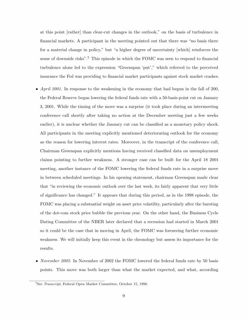
at this point [rather] than clear-cut changes in the outlook,” on the basis of turbulence in

financial markets. A participant in the meeting pointed out that there was “no basis there

for a material change in policy,” but “a higher degree of uncertainty [which] reinforces the

sense of downside risks”.5 This episode in which the FOMC was seen to respond to financial

turbulence alone led to the expression “Greenspan ‘put’,” which referred to the perceived

insurance the Fed was providing to financial market participants against stock market crashes.

• April 2001. In response to the weakening in the economy that had begun in the fall of 200,

the Federal Reserve began lowering the federal funds rate with a 50-basis-point cut on January

3, 2001. While the timing of the move was a surprise (it took place during an intermeeting

conference call shortly after taking no action at the December meeting just a few weeks

earlier), it is unclear whether the January cut can be classified as a monetary policy shock.

All participants in the meeting explicitly mentioned deteriorating outlook for the economy

as the reason for lowering interest rates. Moreover, in the transcript of the conference call,

Chairman Greenspan explicitly mentions having received classified data on unemployment

claims pointing to further weakness. A stronger case can be built for the April 18 2001

meeting, another instance of the FOMC lowering the federal funds rate in a surprise move

in between scheduled meetings. In his opening statement, chairman Greenspan made clear

that “in reviewing the economic outlook over the last week, its fairly apparent that very little

of significance has changed.” It appears that during this period, as in the 1998 episode, the

FOMC was placing a substantial weight on asset price volatility, particularly after the bursting

of the dot-com stock price bubble the previous year. On the other hand, the Business Cycle

Dating Committee of the NBER later declared that a recession had started in March 2001

so it could be the case that in moving in April, the FOMC was foreseeing further economic

weakness. We will initially keep this event in the chronology but assess its importance for the

results.

• November 2002. In November of 2002 the FOMC lowered the federal funds rate by 50 basis

points. This move was both larger than what the market expected, and what, according

5See Transcript, Federal Open Market Committee, October 15, 1998.

9

to the updated RR-04 Greenbook series, was warranted by the available economic data.

Moreover, incoming data received after the completion of the Greenbook “were very close to

our expectations and require little change to [the] near-term forecast.” Particularly in light of

developments in Japan, which had been experiencing persistent deflation since the late 1990s,

it appears that concerns about deflation loomed large.6 Geopolitical risks – preparations

for the 2003 Iraq war were already under way – were also a concern.7 Once again, risk

management considerations motivated a larger-than-usual cut that would provide ‘insurance

against downside risks.” As Chairman Greenspan argued, “if we move significantly today

–and my suggestion would be to lower the funds rate 50 basis points- it is possible that such a

move may be a mistake. But it’s a mistake that does not have very significant consequences.

On the other hand, if we fail to move and we are wrong, meaning that we needed to, the cost

could be quite high.”8

To summarize, by cross-checking the updated Greenbook residual series from RR-04, the

high-frequency series from GSS, and the transcripts from the meetings of the FOMC, we have

identified eight events for which there appears to be a good case that a monetary policy shock

occurred. Of these, four were contractionary, or tightening, shocks (positive in terms of their impact

on the federal funds rate) and four were expansionary, or easing, shocks (negative shocks). We will

therefore consider the following restrictions:

Narrative Sign Restriction 6. The monetary policy shock for the observations corre-

sponding to April 1974, October 1979, December 1998 and February 1994 must be of positive value.

The monetary policy shock for the observations corresponding to December 1990, October 1998,

April 2001 and November 2002 must be of negative value.

Narrative Sign Restriction 7. For the periods specified by Restriction 6, monetary pol-

6One participant expressed concern that “a negative demand shock could cause the disinflation trends we’ve hadlately to morph into deflation,” and staff simulations placed a 25-30% probability that the economy would experiencea deflation. Chairman Greenspan remarked that “if we were to fail to move and the economy began to deteriorate [...]we were looking into a deep deflationary hole.” See Transcript, Federal Open Market Committee, November 6, 2002.

7See Statement, Federal Open Market Committee, November 6, 2002.8See Transcript, Federal Open Market Committee, November 6, 2002.

10

icy shocks are the most important contributor to the observed unexpected movements in the federal

funds rate. In other words, the absolute value of the contribution of monetary policy shocks is larger

than the absolute value of the contribution of any other structural shock.

In terms of the definitions of Section 3, Restriction 6 is a restriction on the sign of the

structural shocks, whereas Restriction 7 is a Type I restriction on the historical decomposition.

Appendix B describes the functions F(Θ) and the matrices Sj necessary to implement Restrictions

6 and 7. In addition, given that for the Volcker episode the evidence is stronger, as in the previous

section we will additionally consider the stronger Type II variant. We repeat Restriction 5 here for

convenience:

Narrative Sign Restriction 5. For the observation corresponding to October 1979, a

monetary policy shock is the overwhelming driver of the unexpected movement in the federal funds

rate. In other words, the absolute value of the contribution of monetary policy shocks to the

unexpected movement in the federal funds rate is larger than the sum of the absolute value of the

contributions of all other structural shocks.

C.1 Results

Figure C.2 presents the IRFs to a monetary policy shock, with and without narrative information.

The gray shaded area represents the 68% (point-wise) confidence bands for the IRFs and the solid

blue lines are the median IRFs using the baseline identification. These results replicate the IRFs

depicted in Figure 6 of Uhlig (2005). The pink shaded areas and red solid lines display the equivalent

quantities when Restrictions 5-7 are also used. The results are very similar to those using only the

Volcker Episode, reported in Figure 8 in the main text.

Table C.1 looks at the probability that the baseline model violates the narrative restrictions,

individually and jointly. Looking at the last column of the table, it can be seen that the baseline

model disagrees with the narrative information for most of the episodes with a very high probability.

11

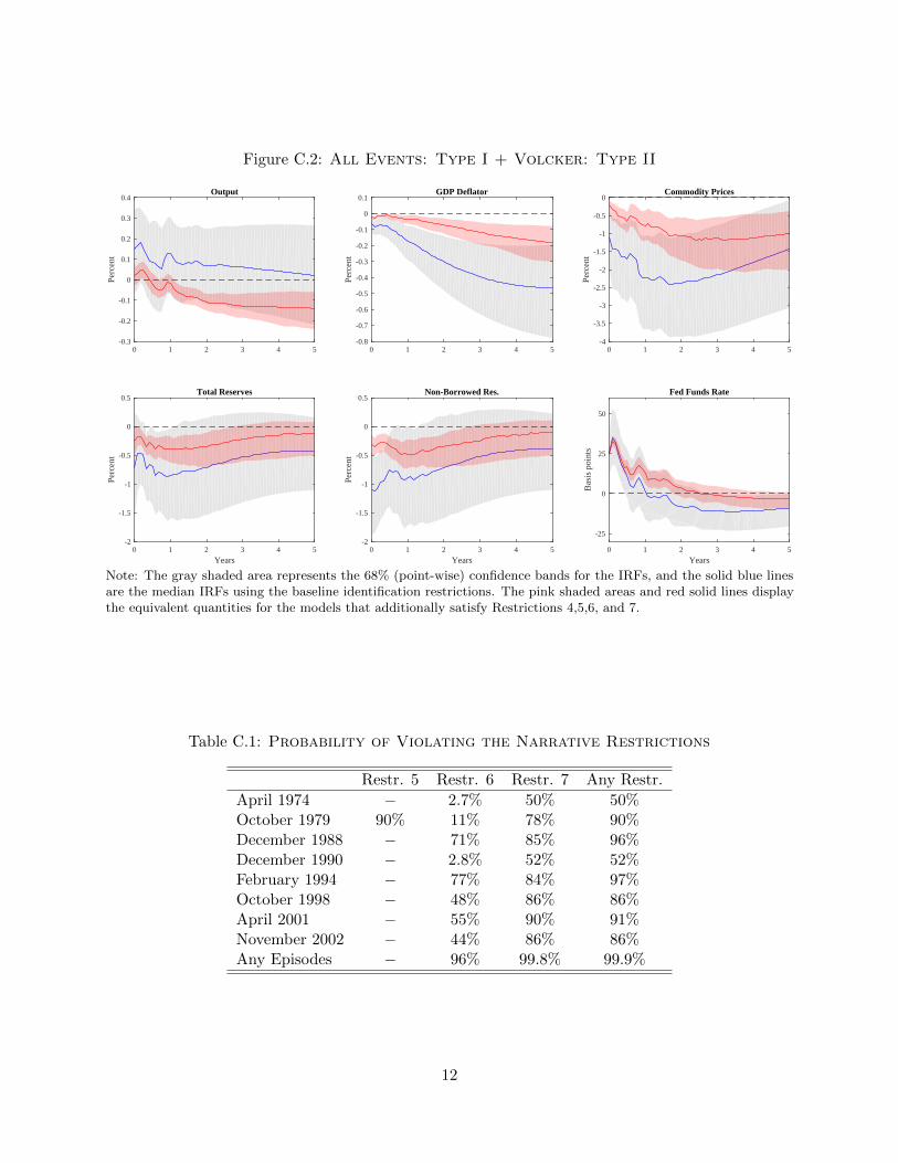
Figure C.2: All Events: Type I + Volcker: Type II

Output

0 1 2 3 4 5

Perc

ent

-0.3

-0.2

-0.1

0

0.1

0.2

0.3

0.4GDP Deflator

0 1 2 3 4 5Pe

rcen

t-0.8

-0.7

-0.6

-0.5

-0.4

-0.3

-0.2

-0.1

0

0.1Commodity Prices

0 1 2 3 4 5

Perc

ent

-4

-3.5

-3

-2.5

-2

-1.5

-1

-0.5

0

Total Reserves

Years0 1 2 3 4 5

Perc

ent

-2

-1.5

-1

-0.5

0


Years0 1 2 3 4 5

Perc

ent

-2

-1.5

-1

-0.5

0

0.5Fed Funds Rate

Years0 1 2 3 4 5

Bas

is p

oint

s

-25

0

25

50

Note: The gray shaded area represents the 68% (point-wise) confidence bands for the IRFs, and the solid blue linesare the median IRFs using the baseline identification restrictions. The pink shaded areas and red solid lines displaythe equivalent quantities for the models that additionally satisfy Restrictions 4,5,6, and 7.

Table C.1: Probability of Violating the Narrative Restrictions

Restr. 5 Restr. 6 Restr. 7 Any Restr.

April 1974 − 2.7% 50% 50%October 1979 90% 11% 78% 90%December 1988 − 71% 85% 96%December 1990 − 2.8% 52% 52%February 1994 − 77% 84% 97%October 1998 − 48% 86% 86%April 2001 − 55% 90% 91%November 2002 − 44% 86% 86%Any Episodes − 96% 99.8% 99.9%

12

narrative sign restrictions for svars - european central bank · a slight modi cation to the...

Documents